Objective Momentum Barriers in Wall Turbulence

Abstract

We use the recent frame-indifferent theory of diffusive momentum transport to identify internal barriers in wall-bounded turbulence. Formed by the invariant manifolds of the Laplacian of the velocity field, the barriers block the viscous part of the instantaneous momentum flux in the flow. We employ the level sets of single-trajectory Lagrangian diagnostic tools, the trajectory rotation average and trajectory stretching exponent, to approximate both vortical and internal wall-parallel momentum transport barrier (MTB) interfaces. These interfaces provide frame-indifferent alternatives to classic velocity-gradient-based vortices and high-shear boundaries between uniform momentum zones (UMZs). Indeed, we find that these elliptic manifold approximations and MTBs outperform standard vortices and UMZ interfaces in blocking diffusive momentum transport, suggesting our momentum barriers are physical features that may be the cause of coherence signatures in statistical and non-objective diagnostics. We also introduce normalized trajectory metrics that provide unprecedented visualizations of objective coherent structures by avoiding strong turbulence biases.

1 Introduction

Early studies of turbulent boundary layer structures were fundamentally inspired by experimentally discovered structures, such as the streaks in boundary layers photographed by Kline et al. (1967) and the typical eddies forming large scale motions described by Falco (1977), shown in Fig. 1. The pioneering bubble, fog and smoke experiments of the 1960’s to 1980’s (see, e.g. Fiedler & Head, 1966; Offen & Kline, 1974; Kline et al., 1967; Falco, 1977; Bandyopadhyay, 1980; Head & Bandyopadhyay, 1981) quantified intermittent material features and boundary layer structures which coherent structure identification methods continue to rely for validation.

Boundary layer tracer experiments suggest an organization of fluid by individual vortices at low Reynolds number, and by packets or collections of vortices as turbulence increases. The $33^{\circ}-45^{\circ}$ angle at which individual vortices extend from the lower boundary has been recreated in multiple experiments for a variety of Reynolds numbers (Falco, 1974; Bandyopadhyay, 1980; Head & Bandyopadhyay, 1981). The diameter of vortex heads has been found to be a fraction of boundary layer height $\delta$ and scales inversely with Re from $0.01\delta-0.2\delta$ (Falco, 1974, 1977). Typical vortices also appear to self-organize into bulges, or large scale motions, with streamwise extent ranging from $1.5-2.5\delta$ (Falco, 1977), which collectively rise at an inclination angle of $18^{\circ}-20^{\circ}$ (Bandyopadhyay, 1980; Head & Bandyopadhyay, 1981). In subsequent hot-wire and particle image velocimetry studies, these ranges of values have been recreated and expanded, but the original measures of material structures remain as the ground-truth for comparison (Adrian, 2007).

Advances in experimental techniques and simulation provided highly resolved velocity fields that stimulated the development of quantitative criteria for the identification of structures seen in tracer experiments (Adrian, 2007). Some of these criteria extract isosurfaces of velocity components to define uniform momentum zones (UMZs), while others employ diagnostic scalar fields, such as the $Q$-, $\lambda_{2}$-, $\Delta$- and $\lambda_{ci}$-parameters, to define vortices (Adrian et al., 2000b; Hunt et al., 1988; Jeong & Hussain, 1995; Zhou et al., 1999; Gao et al., 2011). Yet other approaches identify a relevant temporal or spatial scale and employ a conditional averaging prior to feature extraction (see Dennis & Nickels, 2011; Gul et al., 2020).

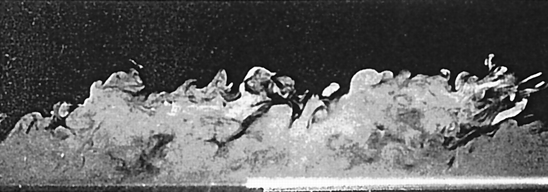
Figure 1: Material wall-bounded turbulent structures visualized with smoke. Reproduced from Falco (1977) with the permission of AIP Publishing.

UMZs were first documented in the early experimental study of Meinhart & Adrian (1995), leading to the seminal work of Adrian et al. (2000b) who suggested that wall-bounded turbulence may be described as a collection of layered zonal structures distinguished by their common streamwise velocities. These structures appear between rapid changes in streamwise velocity across strong shear regions where spanwise vorticity may be concentrated. The relevance of these jumps has been supported by analogous jumps in streamwise velocity at turbulent/non-turbulent interfaces and by nearby hairpin vortices and other vortical features. The core statistical methods used to make these inferences about UMZs and their boundaries were developed by Adrian et al. (2000b) with additional modifications proposed by De Silva et al. (2015); Eisma et al. (2015); Laskari et al. (2018); Fan et al. (2019) and others. With the help of these tools, UMZs have been investigated in a number of wall-bounded flows, including turbulent boundary layers, channel flows and pipe flows at various Reynolds numbers (Adrian et al., 2000b; Kwon et al., 2014; De Silva et al., 2015, 2017; Gul et al., 2020). UMZs have also been widely used as tools to validate other models (Saxton-Fox & McKeon, 2017; Bautista et al., 2019) and generate descriptions of wall-turbulence organization (Adrian, 2007; Hwang & Sung, 2018).

Despite these advances, several practical issues are known with the currently used probability-based UMZ identification scheme, including its sensitivity to the size of the domain, to the number of velocity vectors used in identifying significant velocities (and thus extension to three-dimensional data), and to the number of bins used to reveal streamwise velocity peaks. Two more fundamental issues, however, also arise. First, the broadly hypothesized role of UMZs as fundamental turbulence-organizing zonal-like structures that influence the wall-transverse transport of streamwise linear momentum is often cited but has not yet been directly verified (e.g., Westerweel et al., 2009; Eisma et al., 2015; De Silva et al., 2017; Fan et al., 2019). While it is common for researchers to discuss these zonal-structures, and their probable physical importance, there is currently limited understanding of the momentum transport they induce (Montemuro et al., 2020). Nibbling, engulfment, and entrainment are often studied as influential processes for mass and momentum flux, but fluxes through UMZ interfaces are typically estimated indirectly through conditional sampling and average Reynolds stress profiles. Second, the topology of streamwise velocity level sets (UMZ interfaces) is not objective, i.e., depends on the frame of reference of the observer. This is at odds with the tracer patterns arising in foundational tracer experiments (e.g., Kline et al., 1967; Falco, 1977; Head & Bandyopadhyay, 1981) that originally inspired the study of UMZs, given that those patterns are material and hence are inherently frame-indifferent. Additionally, level-set approaches that rely on Reynolds decompositions, including those in quadrant and octant analysis, introduce a non-physical distortion of the reference frame when different averages are subtracted from each grid cell (Adrian et al., 2000a; Kwon et al., 2016; Saxton-Fox & McKeon, 2017).

One might dismiss the concern about observer dependence by saying that a correct understanding of UMZs in the frame of the experiment is sufficient. The problem with this argument is that a description of features tied to material observations cannot be correct if it only holds in the current frame of observation, whether or not one ever intends to change that frame. More broadly speaking, truly unsteady flows may have convenient frames but have no distinguished frames, as already noted by Lugt (1979). This is the reason why objectivity (or indifference to Euclidean coordinate changes) as a litmus test for flow feature identification was already proposed in the 1970’s (Drouot & Lucius, 1976; Drouot, 1976; Astarita, 1979; Lugt, 1979), prompting a number of recent approaches to adopt observer-indifference as a minimal requirement in coherent structure detection (see Haller, 2005, 2015; Peacock et al., 2015; Kirwan, 2016; Günther & Theisel, 2018, for reviews).

Descriptions of experimentally observed vortical features within and surrounding UMZs (e.g. Head & Bandyopadhyay, 1981) also face objectivity as a minimal self-consistency requirement. Yet the $Q$-, $\lambda_{2}$-, $\Delta$- and $\lambda_{ci}$-isosurfaces used for this purpose are not objective and hence their predictions for observed material tracer patterns, or momentum transport blocking, cannot be accurate (see Haller, 2005, 2021). While correlations may exist between measured scalar concentrations and the features of these non-objective diagnostics (e.g. Westerweel et al., 2009; Eisma et al., 2021), there can be no causal relationship. Several formal modifications of these vortex diagnostics have been proposed to make them objective, but only the approach of Liu et al. (2019a, b) would be generally applicable, as found by Haller (2021). Yet, for lack of a direct connection to material mixing and transport, even correct objectivizations of the currently used $Q$-, $\lambda_{2}$-, $\Delta$- and $\lambda_{ci}$-procedures for vortex identification would depend on their users. Indeed, the users of these procedures are expected to pick values for visualized isosurfaces based on their own expectations for the results (see, e.g., Dubief & Delcayre, 2000). This commonly used approach results in a subjective view of the flow, as recently highlighted by Dong & Tian (2020).

In a parallel development, objective mathematical descriptions of long-term and short-term material deformation have lead to the notions of Lagrangian coherent structures (or LCS) and objective Eulerian coherent structures (or OECS) (see, e.g., Haller, 2015; Serra et al., 2017; Beron-Vera et al., 2018; Serra et al., 2020). Some of these approaches have been used to identify vortices away from turbulent/non-turbulent interfaces (TNTIs) in gravity current experiments (Neamtu-Halic et al., 2019), as well as to look at boundary layer structures in PIV studies (Green et al., 2007; Pan et al., 2009; Wilson et al., 2013; He et al., 2016; Eisma et al., 2021). LCSs and OECSs are, however, constructed as boundaries of coherent structures in passive tracer advection rather than minimizers of momentum transport, as would be required for a physical UMZ interface analog.

Recently, Haller et al. (2020) developed a theory of objective material barriers for the transport of active vector fields, such as vorticity and momentum. These active barriers are sought as material surfaces that block an objectively-defined transport of momentum or vorticity more than any other neighboring material surface. Solving this optimization problem leads to an associated steady, three-dimensional (3D), incompressible dynamical system (the barrier equation) whose structurally stable stream surfaces (invariant manifolds) are precisely the active transport barriers. Haller et al. (2020) showed how active versions of LCS diagnostics, such as the active finite-time Lyapunov exponents (aFTLE) and the active polar rotation angle (aPRA) provide previously unseen levels of detail for momentum-transport barriers in direct numerical simulations of a turbulent channel flow. Instantaneous limits of active material barriers can also be extract via the same machinery. The latter Eulerian barriers are objectively defined surfaces that block the instantaneous flux of the active vector field in question.

Here, we use this recent theory of instantaneous active barriers to define and visualize both momentum trapping vortices and momentum blocking internal interfaces (MTBs) objectively based on their broadly envisioned role as minimizers of momentum transport. To adapt the active barrier field methods to large datasets, and numerically identify large invariant manifolds of the active barrier equations, we use recently developed single-trajectory-based objective coherent structure diagnostics, the trajectory rotation average (TRA) and trajectory stretching exponent (TSE), from Haller et al. (2021). Combining these theories, we develop a simple, systematic procedure that visualizes both MTBs and momentum-trapping vortices in general 3D, wall-bounded turbulence. We also show that the active-barrier-based approach developed here locates vortices and MTB interfaces with significantly lower viscous momentum flux than nearby surfaces obtained from the broadly used velocity-gradient-based vortex diagnostics and non-objective UMZ definition.

2 Methods

2.1 Objective instantaneous barriers to momentum transport

For a 3D fluid velocity field $\mathbf{v}(\mathbf{x},t)$ with density $\rho(\mathbf{x},t)$, the equation of motion can be written as

$$\rho\frac{D\mathbf{v}}{Dt}=-\nabla p+\nabla\cdot\mathbf{T}_{vis}+\mathbf{q},$$ (1)

where $\frac{D}{Dt}$ is the material derivative, $p(\mathbf{x},t)$ is the equilibrium pressure, $\mathbf{T}_{vis}(\mathbf{x},t)$ is the viscous stress tensor, and $\mathbf{q}(\mathbf{x},t)$ contains the external body forces. Fluid trajectories generated by the velocity field $\mathbf{v}$ are solutions, $\mathbf{x}(t;t_{0},\mathbf{x}_{0})$, of the ordinary differential equation $\dot{\mathbf{x}}=\mathbf{v}(\mathbf{x},t)$ with initial position $\mathbf{x}_{0}$ at the initial time $t_{0}$. These fluid trajectories enable the definition of the flow map $\mathbf{F}_{t_{0}}^{t}:\mathbf{x}_{0}\mapsto\mathbf{x}(t;t_{0},\mathbf{x}_{0})$. A material surface $\mathcal{M}(t)$ is then a two-dimensional (2D) manifold,

$$\mathcal{M}(t)=\mathbf{F}_{t_{0}}^{t}[\mathcal{M}(t_{0})],$$ (2)

evolving under the flow map from its initial position $\mathcal{M}(t_{0})$.

To identify exceptional momentum-transport minimizing surfaces, we must first agree on a definition of frame-indifferent momentum flux. As pointed out by Haller et al. (2020), the broadly used linear momentum flux

$$\mathrm{Flux}_{\rho\mathbf{v}}(\mathcal{M}(t))=\int_{\mathcal{M}(t)}\rho\mathbf{v}(\mathbf{v}\cdot\mathbf{n})dA$$ (3)

is unsuitable for systematic, observer-independent momentum-flux measurements through a material surface $\mathcal{M}(t)$ for several reasons. First, this flux expression originally arises from the application of the Reynold transport theorem to quantify linear momentum carried by fluid trajectories through a non-material control surface. No such trajectory crossings are, however, possible through a material surface. Second, a flux of a quantity through a surface should have the units of that quantity divided by time and multiplied by the surface area, which is not the case for $\mathrm{Flux}_{\rho\mathbf{v}}$. Third, $\mathrm{Flux}_{\rho\mathbf{v}}$ is not objective because under Euclidean coordinate changes of the form

$$\mathbf{x}=\mathbf{Q}(t)\mathbf{y}+\mathbf{b}(t),\qquad\mathbf{Q}\mathbf{Q}^{T}=\mathbf{I},$$ (4)

the integrand in (3) does not transform as an objective velocity field, i.e., we have $\mathbf{v}(\mathbf{v}\cdot\mathbf{n})\neq\mathbf{Q}\tilde{\mathbf{v}}(\tilde{\mathbf{v}}\cdot\tilde{\mathbf{n}})$ for the transformed velocity field

$$\tilde{\mathbf{v}}=\mathbf{Q}^{T}\left(\mathbf{v}-\dot{\mathbf{Q}}\mathbf{y}-\dot{\mathbf{b}}\right).$$

This observer dependence is equally true for fluxes obtained from conditionally-averaged entrainment velocities used in TNTI studies (e.g. Westerweel et al., 2009; Da Silva et al., 2014; Eisma et al., 2015), as well as projections of momentum flux in the streamwise direction.

To address these shortcomings of $\mathrm{Flux}_{\rho\mathbf{v}}$, Haller et al. (2020) introduce a frame-indifferent flux for an arbitrary, dynamically active vector field $\mathbf{f}(\mathbf{x},t)$ that satisfies a partial differential equation of the form

$$D\mathbf{f}/Dt=\mathbf{h}_{vis}+\mathbf{h}_{nonvis}\qquad\partial_{\mathbf{T}_{vis}}\mathbf{h}_{vis}\neq 0\qquad\partial_{\mathbf{T}_{vis}}\mathbf{h}_{nonvis}=0.$$ (5)

Here the term $\mathbf{h}_{vis}(\mathbf{x},t,\mathbf{v},\mathbf{f},\mathbf{T}_{vis})$, arising from diffusive forces (i.e., viscous Cauchy-stresses), is assumed to be an objective vector field, i.e., $\mathbf{h}_{vis}=\mathbf{Q}\tilde{\mathbf{h}}_{vis}$. The other term, $\mathbf{h}_{nonvis}(\mathbf{x},t,\mathbf{v},\mathbf{f})$, is assumed to have no explicit dependence on viscous forces. Instead, it contains terms originating from the pressure, external forces and possible inertial effects. For instance, if $\mathbf{f}$ is the linear momentum of an incompressible Navier–Stokes flow with kinematic viscosity $\nu$, then the Navier–Stokes equations directly imply

$$\mathbf{h}_{vis}=\rho\nu\Delta\mathbf{v},$$ (6)

which is an objective vector field, because $\Delta\mathbf{v}=\mathbf{Q}\Delta\tilde{\mathbf{v}}$.

The diffusive flux of $\mathbf{f}(\mathbf{x},t)$ through $\mathcal{M}(t)$ can then be defined as the surface integral of the diffusive part of the surface-normal material derivative of $\mathbf{f}\left(\mathbf{x},t\right)$ over $\mathcal{M}(t)$:

$$\Phi\left(\mathcal{M}(t)\right)=\left[\int_{\mathcal{M}(t)}\frac{D\mathbf{f}}{Dt}\cdot\mathbf{n}\,dA\right]_{vis}=\int_{\mathcal{M}(t)}\mathbf{h}_{vis}\cdot\mathbf{n}\,dA.$$ (7)

In contrast to eq. (3), the diffusive momentum flux $\Phi\left(\mathcal{M}(t)\right)$ has the correct physical units of momentum flux and is objective. Indeed, under all observer changes of the form (4), we obtain $\mathbf{h}_{vis}\cdot\mathbf{n}\,dA=\left(\mathbf{Q}\tilde{\mathbf{h}}_{vis}\right)\cdot\left(\mathbf{Q}\tilde{\mathbf{n}}\right)d\tilde{A}=\tilde{\mathbf{h}}_{vis}\cdot\tilde{\mathbf{n}}\,d\tilde{A}$.

We also define a measure, $\Phi_{N}$, that is focused solely on quantifying the amount of tangency a surface $\mathcal{M}(t)$ shares with a diffusive momentum flux barrier:

$$\Phi_{N}\left(\mathcal{M}(t)\right)=\int_{\mathcal{M}(t)}\frac{\mathbf{h}_{vis}}{||\mathbf{h}_{vis}||}\cdot\mathbf{n}\,dA.$$ (8)

In flows with a wide range of $\mathbf{h}_{vis}$ magnitudes, $\Phi_{N}$ provides a normalized measure with no preferential bias towards low-magnitude regions of the flow.

By formula (7), a material surface $\mathcal{M}(t)$ is a perfect instantaneous barrier to diffusive momentum flux if $\mathbf{h}_{vis}\cdot\mathbf{n}$ (and thus ${||\mathbf{h}_{vis}||}^{-1}(\mathbf{h}_{vis}\cdot\mathbf{n})$) vanishes at each point of $\mathcal{M}(t)$. In other words, the surface $\mathcal{M}(t)$ must be tangent to the vector field $\mathbf{h}_{vis}$ at each of its points, i.e., $\mathcal{M}(t)$ must be an invariant manifold of the differential equation $\mathbf{x}^{\prime}=\mathbf{h}_{vis}$ . Here prime denotes differentiation with respect to the barrier time, $s$, which parameterizes trajectories of this differential equation.

Specifically, when $\mathbf{f}$ is the linear momentum, then we obtain from 6 that $\mathcal{M}(t)$ is an invariant manifold of the instantaneous momentum barrier equation

$$\mathbf{x}^{\prime}(s)=\Delta\mathbf{v}(\mathbf{x}(s),t).$$ (9)

Here, to speed up trajectory integration, we have dropped the small scalar factor $\rho\nu$ in the definition of $\mathbf{h}_{vis}$ in (6). This has no impact on the invariant manifolds (stream surfaces) of $\mathbf{h}_{vis}$.

The barrier time $s$ is a non-dimensional geometric parameter along trajectories of the barrier equations. As such, it has no direct fluid dynamical meaning, much the same way as the geometric parameter $\tau$ has no direct physical meaning in the differential equation $dx/d\tau=v(x,t)$ defining the instantaneous streamlines of a velocity field. However, if we normalize the barrier vector field to a unit vector at each point, then $s$ will measure precisely the arclength of a computed barrier trajectory. In that case, setting a maximal value $s^{*}$ for $s$ in our calculations will directly control the barrier length scales revealed by the Lagrangian diagnostics computed on the barrier equations up to the barrier time $s^{*}$.

Even at the Reynolds numbers considered here, the diffusive momentum transport is small relative to the total momentum transport, which is dominated by pressure-induced transport. The ratio between diffusive and pressure-induced momentum transport decreases further with increasing Reynolds numbers. We propose, however, that coherent structure boundaries in the flow are distinguished precisely by their ability to inhibit the diffusive component of the momentum transport. Indeed, the transport induced by the pressure gradient also moves coherent structures along with the bulk flow and hence fails to distinguish their boundaries. This view on coherent structure boundaries has been justified analytically for all directionally steady Beltrami solutions of the Navier-Stokes equation, for arbitrary high Reynolds numbers (see Haller et al., 2020). The same principle has been verified numerically for diffusive passive scalar transport by Haller et al. (2018). They find the observed coherent structures in two-dimensional geophysical flows coincide with barriers to the diffusive transport of passive scalars (such as the scalar vorticity) for arbitrarily small diffusion.

As further illustration in the Appendix, we compare perfect barriers to the diffusive momentum transport and perfect barriers to the total momentum transport for an exact Navier-Stokes solution, the time-dependent ABC flow. Due to the dominance of the strongly compressible pressure gradient vector field, the barrier surfaces to total momentum transport accumulate on each other and spiral into fixed points. These characteristically dissipative surfaces are notably dissimilar to the coherent structures seen in tracer experiments and hence would be inconsistent with the view put forward by Westerweel et al. (2009) on the relation between barriers of tracer transport and those of momentum transport.

By construction, any 2D structurally stable invariant manifold $\mathcal{M}(t)$ of the barrier equation (9) represents an exact and dynamically robust instantaneous barrier to the diffusive transport of linear momentum. If $\mathbf{v}$ is incompressible, then the barrier equation (9) is an incompressible, steady dynamical system, given that the time $t$ only plays the role of a parameter (which temporal frame to investigate) and the right-hand side of (9) has no explicit dependence on the barrier time $s$. Therefore, as is well known from chaotic advection studies of 3D, steady, incompressible flows, structurally stable 2D invariant manifolds of (9) are stable manifolds, unstable manifolds and invariant tori. We note that Haller et al. (2020) also extends the barrier equation (9) to cover material transport barriers over a finite time interval, but here we will focus on instantaneous momentum barriers. Both the instantaneous and the material barrier equations are objective.

Invariant manifolds (or distinguished stream surfaces) of the barrier equation (9) can only be determined numerically and hence will be approximate. We provide two different methods to numerically approximate these barriers with different orders of computational burden. In order to evaluate the accuracy of our computations and compare the momentum-blocking ability of the computed barriers to nearby features obtained from common vortex and UMZ identification procedures, we will use the surface-area-normalized geometric momentum flux across a surface $\mathcal{M}(t)$,

$$\mathrm{\Psi}(\mathcal{M}(t))=\frac{\int_{\mathcal{M}(t)}|\Delta\mathbf{v}\cdot\mathbf{n}|dA}{\int_{\mathcal{M}(t)}dA}.$$ (10)

This objective quantity does not allow for a cancellation of fluxes in opposite directions and hence vanishes only on perfectly computed momentum barriers. As a result, $\mathrm{\Psi}(\mathcal{M}(t))$ provides an objective, nonnegative scalar metric for the permeability of the surface $\mathcal{M}(t)$ with respect to momentum transport irrespective of the size of $\mathcal{M}(t)$.

Similary, the normalized unit barrier field measure,

$$\mathrm{\Psi_{N}}(\mathcal{M}(t))=\frac{\int_{\mathcal{M}(t)}\left|\frac{\Delta\mathbf{v}}{||\Delta\mathbf{v}||}\cdot\mathbf{n}\right|dA}{\int_{\mathcal{M}(t)}dA},$$ (11)

quantifies the degree of tangency between an imperfect barrier and trajectories of the linear momentum barrier field (9). This measure provides a clear comparison for surfaces in distinct regions of a flow with different momentum barrier field vector magnitudes by focusing solely on geometry with no bias for small $\Delta\mathbf{v}$ values. $\mathrm{\Psi_{N}}$, however, does not have the units of flux and is thus referred to as our barrier field tangency measure.

2.2 Identification of momentum barrier surfaces

A number of relevant techniques have been developed in the LCS literature to identify distinguished material surfaces of 3D steady flows from arrays of trajectories (see Haller, 2015, for a review). These methods generally require a numerical differentiation of the flow map or of the velocity field along particle positions. The 3D steady dynamical system (9) already involves two spatial derivatives of the velocity field and further spatial differentiation can only be carried out accurately over sufficiently dense numerical grids (see Haller et al. (2020) for examples involving Cauchy-Green strain tensor based diagnostics).

To avoid the numerical issues associated with further spatial differentiation of solutions of (9) and to reduce the number of integrated trajectories, here we use very recently developed single-trajectory diagnostics for elliptic (i.e., vortex-type) and hyperbolic LCS the trajectory rotation average (TRA) and the trajectory stretching exponent (TSE), derived by Haller et al. (2021). On any discretized trajectory $\left\{\mathbf{x}(s_{i})\right\}_{i=0}^{N}$ of the barrier equation (9) with initial condition $\mathbf{x}(s_{0})=\mathbf{x}(0)=\mathbf{x}$, the TRA measures the temporal average of the angular velocity of the trajectory whereas the TSE measures the average hyperbolicity strength along the trajectory. Evaluated in the context of the barrier equation (9), these two fields can be computed as

$$\mathrm{TRA}_{0}^{s_{N}}(\mathbf{x})=\frac{1}{s_{N}}\sum_{i=0}^{N-1}\cos^{-1}\frac{\left\langle\dot{\mathbf{x}}(s_{i}),\dot{\mathbf{x}}(s_{i+1})\right\rangle}{\left|\dot{\mathbf{x}}(s_{i})\right|\left|\dot{\mathbf{x}}(s_{i+1})\right|}$$ (12)

and

$$\mathrm{TSE}_{0}^{s_{N}}(\mathbf{x})=\frac{1}{s_{N}}\sum_{i=0}^{N-1}\left|\log\frac{\left|\dot{\mathbf{\mathbf{x}}}(s_{i+1})\right|}{\left|\dot{\mathbf{\mathbf{x}}}(s_{i})\right|}\right|.$$ (13)

To simplify our notation, we have omitted the overbar from the $\mathrm{TRA}_{0}^{s_{N}}$ and $\mathrm{TSE}_{0}^{s_{N}}$ which was used by Haller et al. (2021) to distinguish formula (12) and (13) from their versions that allowed for cancellations along trajectories. TRA and TSE computed in (non-objective) physical velocity fields are not objective. In our present context, however, $\mathrm{TRA}_{0}^{s_{N}}(\mathbf{x})$ and $\mathrm{TSE}_{0}^{s_{N}}(\mathbf{x})$ are objective fields, because they are computed along trajectories of the objective barrier vector field $\Delta\mathbf{v}$.

Calculating trajectories in the unit barrier field

$$\mathbf{x}^{\prime}(s)=\frac{\Delta\mathbf{v}(\mathbf{x}(s),t)}{|\Delta\mathbf{v}(\mathbf{x}(s),t)|}$$ (14)

preserves momentum barrier geometry but standardizes the length of all paths for the same advection time, $s_{N}$. TRA and TSE fields calculated from trajectories in the normalized barrier field, NTRA and NTSE, respectively, visualize features in both highly turbulent regions (large $\Delta\mathbf{v}$), and less turbulent flow regions, with equal fidelity. As will be shown in the following sections, NTRA and NTSE provide unprecedented comparisons of objective coherent structures over the full range of scales and strengths present in a turbulent flow, and concurrently reveal additional weak structures in less turbulent regions that are not evident from other Eulerian methods.

Haller et al. (2021) show that fronts and outer boundaries of nested cylindrical level surfaces of the TRA and TSE fields highlight the same hyperbolic and elliptic invariant manifolds as the finite-time Lyapunov exponent (FTLE, Haller (2015)), polar rotation angle (PRA, Farazmand & Haller (2016)) and the Lagrangian-averaged vorticity deviation (LAVD, Haller et al. (2016)), but without relying on the spatial differentiation required by the latter three diagnostics. The TRA and TSE fields are, therefore, computable from sparse data and their local value is independent of the number and proximity of other trajectories used in the analysis. In upcoming visualizations, influential invariant manifolds of the barrier equation will appear as 2D surfaces along which TRA or TSE exhibit large changes. The barrier time $s_{N}$ in (12) and (13) can be selected arbitrarily, as it is independent of the physical time of the flow data. An increase in $s_{N}$ enhances details in TRA and TSE visualizations, enabling a gradual, scale-dependent exploration of invariant manifolds in the phase space of the autonomous system (9).

For arbitrarily large barrier times, however, the quality of visualization begins to degrade. This is caused by barrier field trajectories leaving neighborhoods of the finite-sized codimension-one invariant manifolds influencing their initial paths. As $\mathrm{TRA}$ and $\mathrm{TSE}$ are monotonically non-decreasing functions of $s$, hyperbolic and elliptic manifolds encountered away from trajectory initial positions will have outsized influence and the diagnostics no longer reflect the features at $\mathbf{x}_{0}$. We thus suggest determining $s_{N}$ for a given region $U$ as the decorrelation time of instantaneous $\mathrm{TRA}$ (or $\mathrm{TSE}$) values. Specifically, for each $\mathbf{x}_{0}\in U$, we calculate the first zero of the autocorellation

$$R(\tau,\mathbf{x}_{0}) = \sum_{i=0}^{N-1}(f(s_{i},\mathbf{x}_{0})-\bar{f})(f(s_{i}-\tau,\mathbf{x}_{0})-\bar{f}),\quad\tau\geq 0,$$

$$f(s_{i},\mathbf{x}) = \mathrm{TRA}_{s_{i}}^{s_{i+1}}(\mathbf{x}_{0}),$$ (15)

where $\bar{f}$ is the temporal average of $f$. The median value of this decorrelation time over all $\mathbf{x}_{0}\in U$ provides a suitable integration time to visualize most invariant manifolds of the barrier field in $U$ with limited interference. We use the same method for determining $s_{N}$ for the normalized NTRA and NTSE fields in (14) as well. We have found that decorrelation times for $\mathrm{TRA}$ and $\mathrm{TSE}$ to be approximately equal in our numerical studies.

2.3 Direct numerical simulation data

To facilitate reproducibility and foster further comparisons with future developments, we have selected from the publicly available Johns Hopkins University Turbulence Database (JHTDB) a direct numerical simulation of a $Re_{\tau}=1000$ channel flow (Perlman et al., 2007; Li et al., 2008; Graham et al., 2016). On this data set, we compare UMZ interfaces and velocity-gradient-based vortices with perfect instantaneous barriers to the diffusive transport of linear momentum. While UMZ studies are typically performed on turbulent boundary layers, Kwon et al. (2014) and Fan et al. (2019) have argued for the generalization of such features to channel flows as well.

The JHTDB channel flow data is available on a $2048\hskip 1.49994pt\times\hskip 1.49994pt512\hskip 1.49994pt\times\hskip 1.49994pt1536$ grid for a domain of size $8\pi h\hskip 1.49994pt\times\hskip 1.49994pt2h\hskip 1.49994pt\times\hskip 1.49994pt3\pi h$, where $h$ is the half-channel height. The DNS timestep $\Delta t=0.0013$ in non-dimensional simulation units, with the stored simulation timestep, $\delta t=5\Delta t$, or approximately one channel flow-through time. The analysis herein is conducted over 100 frames spanning the entire simulation database with a duration of 4,000 channel flow-through times from $t=0$ to $t=26$. All figures and analysis will be displayed in non-dimensional half-channel height units ($h=1$). This dataset has been used in a number of studies, most notably by Bautista et al. (2019) to evaluate a model of velocity-based uniform momentum zones, and by Jie et al. (2021) to investigate inertial particle collection in the quiescent core.

To account for the instability caused by numerical integration through large $\Delta\mathbf{v}$ fluctuations near the channel walls, we have implemented a quadratic buffer in the lower viscous sublayer, within 5 viscous lengths or $0.005h$ from the wall. That is, for $0.995h\leq|y|\leq 1$, we define $\Delta\mathbf{v}(x,y)=v(x,\pm 0.995h)(\frac{y\mp 1}{0.995h\mp 1})^{2}$ for the appropriate wall. Eyink et al. (2020) examined this region and calculated these heights to be well within the viscous sublayer for our JHU channel. We find that this minimal buffer zone does not modify the visualization of structure in the momentum barrier field, but it significantly expedites calculations and aids in fixed timestep advection of trajectories at the long time scales necessary for determining optimal decorrelation times in (15).

2.4 Computational consideration

Common to Lagrangian-trajectory diagnostics, the computational burden of calculating TRA and TSE in the vector fields (9) and (14) primarily comes from the accurate integration of trajectories which requires interpolating large vector fields to determine trajectory velocities. The present analysis was conducted in MATLAB on either a professional workstation for specific examples, or a high performance computing cluster to calculate large numbers of TRA and TSE fields in large domains. Using a fourth-order Runge-Kutte integration scheme with 10,000 timesteps on a 2.3 GHz, 18 Core, 128GB iMac Pro, TRA and TSE values from 10,000 initial positions, $\mathbf{x}_{0}$, can be computed in an interpolated vector field of $100\times 100\times 100$ grid points, with spatial dimensions $1.2h\times 0.6h\times 0.6h$, in a wall-clock time of 5 seconds. This can clearly be improved upon in more computationally efficient programming languages.

As one increases the spatial dimensions of initial conditions $\mathbf{x}_{0}$, the flow domain used in the interpolation needs to be increased to avoid boundary effects, as in Eisma et al. (2021). This, in turn, decreases the speed of the computations. We thus calculate the TRA and TSE fields in (9) using a patchwork of initial positions in flow domains with large margins so as to avoid trajectories leaving the domain. In the subsequent analysis, we found exemplary visualization is possible with spatial resolutions on the order of 1 to 10 viscous lengths ($10^{-3}h$ to $10^{-2}h$), with the finer resolutions beneficial for smooth flux-minimizing isosurface extraction. Parallelized MATLAB scripts to calculate TRA and TSE are available on github (https://github.com/haller-group/TRA_TSE).

3 Results

3.1 Objective momentum transport barrier visualization

Figure 2 compares a common turbulence visualization diagnostics, the vorticity magnitude, with the $\mathrm{NTRA}$ field computed for the normalized momentum barrier equation (14) on a streamwise-wall-normal plane of initial conditions in the channel at the non-dimensional DNS time $t=0.065=5\delta t$. The predominant channel flow is in the positive $x$-direction with channel walls at $y=\pm 1$. Both diagnostic fields in Fig. 2 were generated from precisely the same velocity field, and were calculated and visualized at the same spatial resolution ($\delta_{x}=\delta_{y}=10^{-3}$). The vorticity picture is indicative of the scale and resolution of structures that are captured by velocity and velocity-gradient-based level-set methods. The barrier trajectories $\mathbf{x}(s)$ used in these simulations were advected under the 3D normalized barrier equation until $s_{N}=0.5$, the order of decorrelation time for the entire channel.

The shear generated by the upper and lower channel walls is evident from the high rates of trajectory rotation and vorticity. Surprisingly, in the NTRA field, there is strong evidence of many more vortical momentum barriers in the center of the channel, which is typically viewed as a quiescent region. This shows that while there are still many complex vortex interactions occurring in the region, their relatively weaker signature makes them impossible to identify in the weak gradients and uniformly low vorticity values. Thus, the NTRA field provides an enhanced visualization of structures at a much wider range of spatial scales and structure strengths for the same underlying velocity data. For identifying boundaries and the structure extraction discussed in the next sections, we find the large changes evident in TRA and TSE fields to be most beneficial. At the same time, NTRA and NTSE continue to provide homogeneous fidelity visualizations of barriers in large domains that contain a wide range of vector magnitudes.

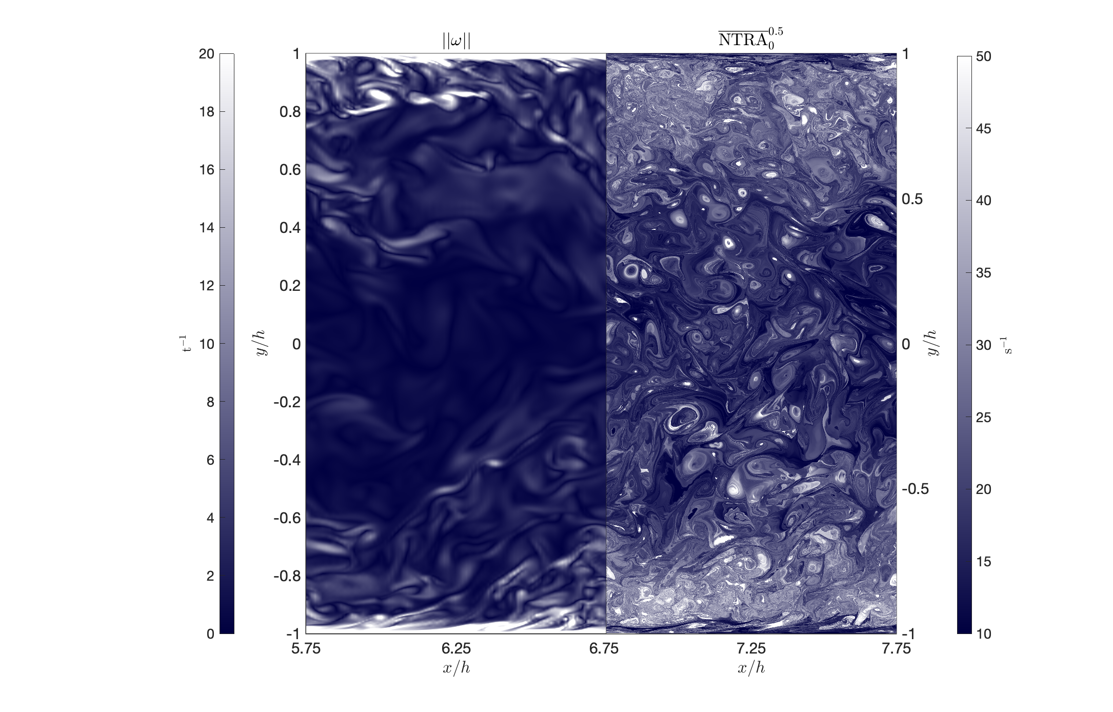
Figure 2: A streamwise-wall-normal plane of the $Re_{\tau}=1000$ JHTDB Channel Flow colored by vorticity magnitude (left) and $\mathrm{\overline{NTRA}}_{0}^{0.5}$ (right). Both visualizations of turbulent features were calculated at the same spatial resolution from the same velocity data at one time step. The enhanced visualization possible with $\overline{\mathrm{NTRA}}$ provides a striking comparison with classic techniques and illuminates faint and weak structure in the center of the channel while maintaining objectivity.

Zooming in on the turbulent wall-region, we find the degree of detail of TRA fields for the original barrier equations (9) is also unattainable by classic velocity-gradient based vortex diagnostics. This first-order benefit can be seen in Fig. 3, in which TRA is compared with $Q$, $\lambda_{2}$, and $\lambda_{ci}$ (swirling strength) (Hunt et al., 1988; Jeong & Hussain, 1995; Zhou et al., 1999) for a streamwise-wall-normal ($x$,$y$) plane adjacent to the lower channel wall. Again, all four plots were generated with the same spatial resolution from the same single velocity snapshot of the DNS data. In contrast to the other plots, the TRA is objective and reveals substantially more of the complexity of the flow for the decorrelation advection time $s_{N}=10^{-4}$.

The TRA plot in Fig. 3 reveals a complex connection network and a layering of unique rotational features not present in the velocity-gradient-based diagnostics. All colormaps have been chosen to reveal the full range of metric values, though gradient-based approaches suffer from the same issues as in Figure 2. The level of detail in the TRA field provides increased accuracy in vortex detection. For example, at approximately $(x/h,y/h)=(0.8,-0.9)$, there is a clear maximum in all three velocity-gradient-based metrics, suggesting the potential presence of a coherent vortex (yellow box). Upon closer inspection of the TRA in the same region, however, we find a lack of nested cylindrical TRA level surfaces. Instead, filamenting invariant surfaces of the barrier equation are present that are not structurally stable and hence do not define vortical barriers to momentum transport. The TRA field discerns these important structural features and has a significant advantage in preventing false-positive vortex identifications. Furthermore, these details are useful for accurately tracking individual features from one time to the next, as will be discussed in Section 3.4. An internal layering close to the wall is also present in the TRA field, as is the organization of vortices around a clearer transition between the more turbulent wall region and the less turbulent channel core. We discuss this interface in more detail in the Section 3.3.

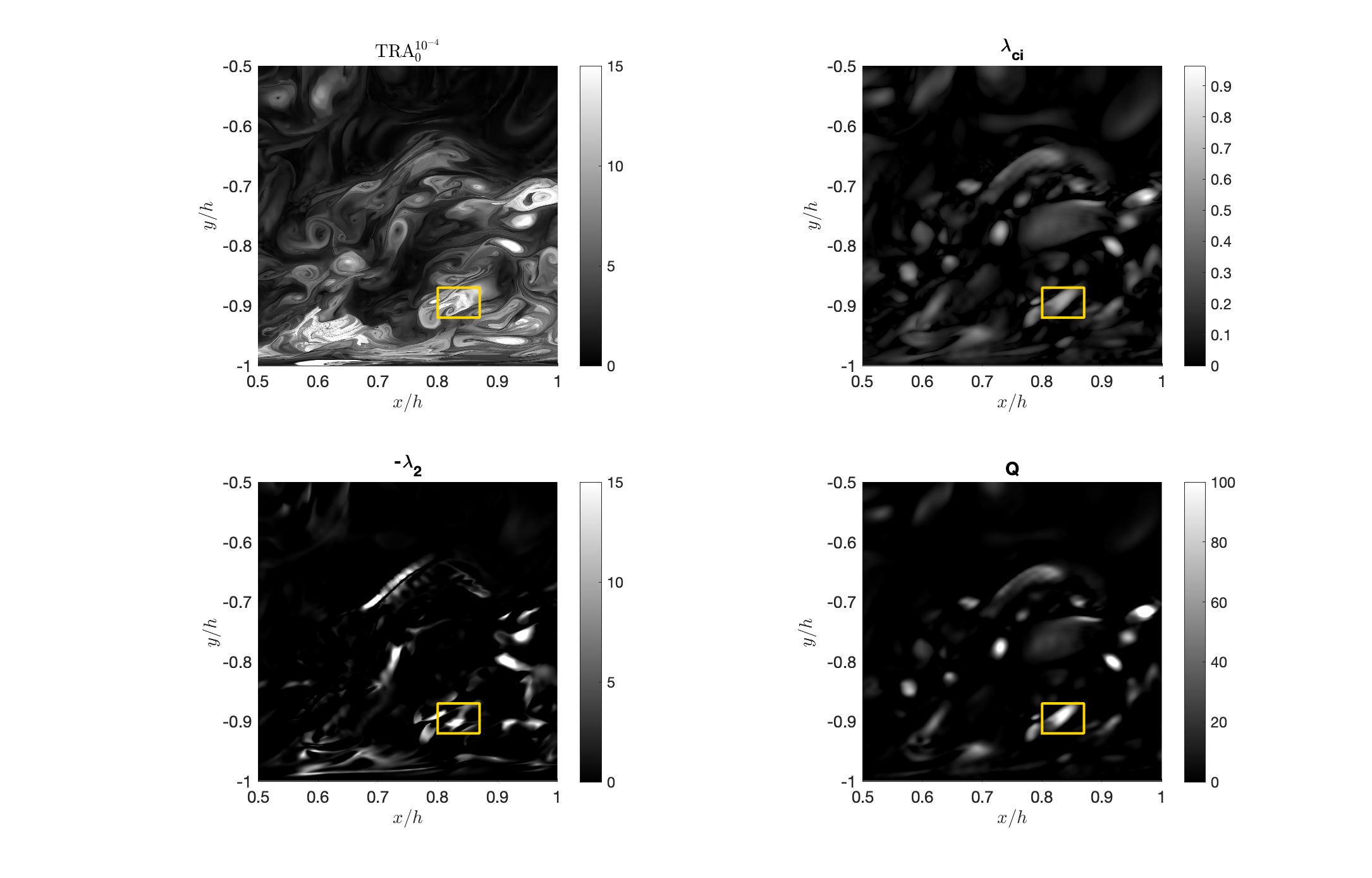
Figure 3: Comparison of the objective TRA field with non-objective, velocity-gradient-based vortex identification diagnostics in the highly turbulent region at the channel wall. All four plots were computed with the same spatial resolution from the same single velocity snapshot of the DNS data.

3.2 Momentum-trapping vortices

In 2D cross-sections of the flow, vortex boundaries can be located as outermost members of nested families of closed level curves of the TRA. Launching trajectories of the 3D barrier equation (9) from these boundary curves generates instantaneous, vortical momentum barrier surfaces in the full 3D flow. In direct contrast to velocity-gradient-based vortex identification practices, this process is devoid of any user-defined parameters beyond a choice of spatial resolution of barrier-field trajectory initial positions, which only serves to control the level of detail in the TRA field. In contrast to velocity and velocity-gradient-based diagnostics, increasing the spatial resolution of TRA and TSE fields beyond that of the underlying velocity field can continue to increase the structural information revealed because of the dummy time barrier field integration.

Figure 4 shows one example of our momentum-trapping vortex identification method, with barrier trajectories starting from the $z=2.55h$ plane. The left panel also reveals a strong similarity between the detailed structures in the TRA field and the material boundary layer structures visualized in smoke experiments (Fig. 1), to be discussed in more detail in Section 3.4.

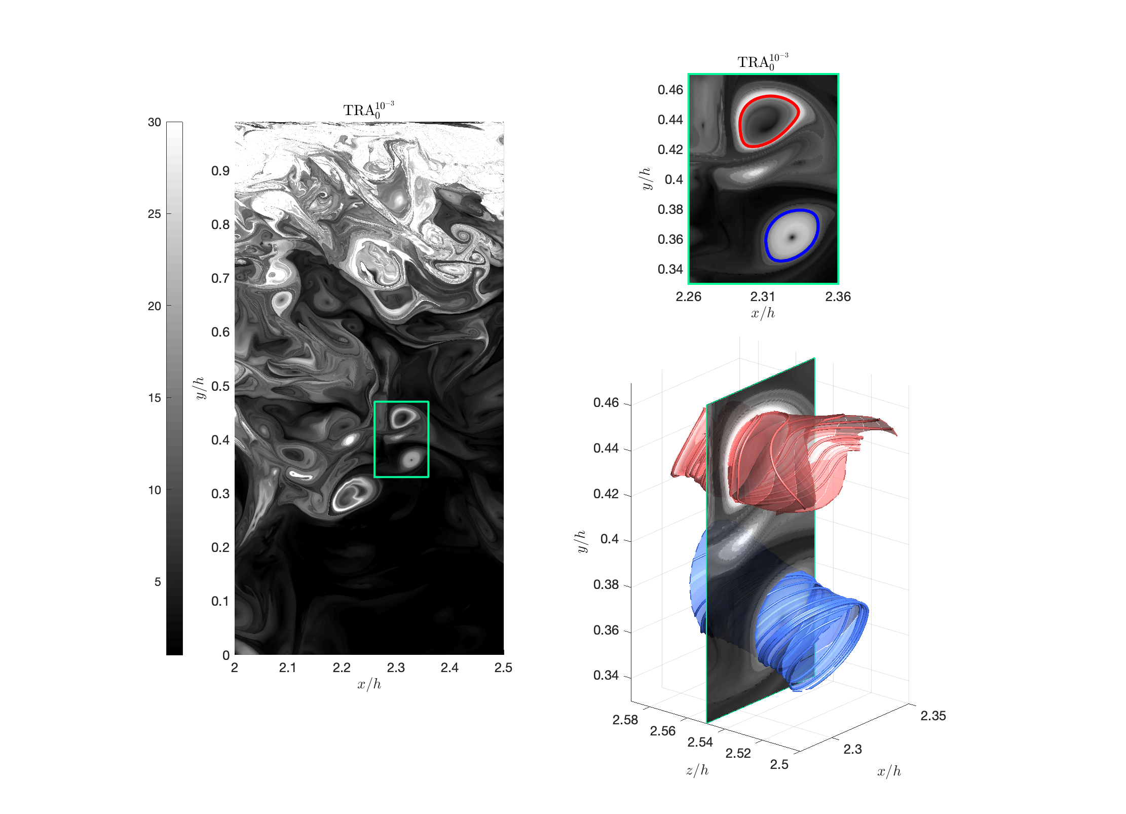
Figure 4: Momentum-trapping vortices in the turbulent channel flow. The vortex boundaries are determined as streamsurfaces of $\Delta\mathbf{v}$ that intersect the plane of investigation ($z=2.55$) along outermost closed and convex TRA contours.

Through a simple search algorithm on TRA contours, we have identified a region with a nested set of closed TRA level curves. By extracting all TRA contours that that span the range of values present, we can isolate the closed and convex contours. The outermost convex boundary curve for each vortex obtained in this fashion is highlighted in the top right of Fig. 4. Using these vortex boundaries as initial positions, we can advect a dense set of trajectories in the barrier field in forward and backward barrier time to obtain the exact momentum transport barriers seen in the bottom right. If choosing smaller members of the set of closed level curves of the TRA as a curve of initial conditions, we obtain an internal foliation of the vortex by smaller cylindrical momentum barriers. These block radial diffusive momentum transport within the vortex. The details of this process are described in Algorithm 1.

	Algorithm 1: Extracting momentum vortex cores
1	For a co-dimension 0 domain of interest $U\subset\mathbb{R}^{3}$, select a grid of initial conditions $\mathbf{x}_{0}\in U$.
2	Choose an initial barrier time estimate $\epsilon$ and calculate the discretized trajectories $\left\{\mathbf{x}(s_{i})\right\}_{i=0}^{N}$ in the barrier field (9) where $\epsilon=s_{N}$.
3	For each trajectory $\mathbf{x}(s_{i})_{i=0}^{N}$, calculate $f(s_{i},\mathbf{x})$ following (15) and (12).
4	Determine the optimal barrier time $\epsilon_{0}$ as the first-zero crossing of the autocorrelation of $f$ as defined in (15). If no zero-crossing exists, repeat Steps 2-4 with progressively larger $\epsilon$ until a zero-crossing exists.
5	Repeat Steps 1-2 for $\epsilon_{0}=s_{N}$ and calculate $\mathrm{TRA}_{0}^{s_{N}}$ following (12).
6	Select a plane of interest of initial conditions that intersects $U$ and extract iso-contours in that plane for the range of TRA values generated in Step 5. Record only the outermost closed convex contours $\left\{\gamma_{j}\right\}$ as vortex core candidates.
7a	To extract the invariant manifold of (9) that intersects a given curve $\gamma_{j}$ , identify trajectories $\left\{\mathbf{x}_{\gamma_{j}}(s_{i})\right\}_{i=0}^{N}$ such that $\mathbf{x}_{\gamma_{j}}(0)\in\gamma_{j}$. If an insufficient number of trajectories exist, identify points in $\gamma_{j}$ through interpolation to obtain a set $\mathbf{x}_{\gamma_{j}}(0)$ and repeat Step 2 with $s_{N}=\epsilon_{0}$.
7b	Given a sufficiently dense set of trajectories, the co-dimension 1 vortex core be identified by linear interpolation between nearest points in the set of trajectory data $\left\{\mathbf{x}_{\gamma_{j}}(s_{i})\right\}_{i=0}^{N}\in\mathbb{R}^{3}$.
8a	To obtain a level-surface approximation of a momentum vortex core that intersects a given closed contour $\gamma_{j}$, extract that TRA isosurface $\mathcal{I}_{\mathrm{TRA}}$ that intersects $\gamma_{j}$.
8b	Repeat 7a and calculate the distance between points in $\mathcal{I}_{\mathrm{TRA}}$ and nearest points in $\left\{\mathbf{x}_{\gamma_{j}}(s_{i})\right\}_{i=0}^{N}$.
8c	Calculate the PDF of these distances. $\mathcal{I}_{\mathrm{TRA}}$ will be sufficiently close to $\left\{\mathbf{x}_{\gamma_{j}}(s_{i})\right\}_{i=0}^{N}$ for many points, resulting in a distinct peak in the PDF near zero. Refine $\mathcal{I}_{\mathrm{TRA}}$ to only include points in this near-zero peak
9	Steps 5-8 can be repeated for $-\epsilon_{0}$ to further expand the extracted vortex core.

A simpler but only approximate way to visualize objective momentum barriers is to plot level surfaces of the TRA field. This is inspired by the observation that structurally-stable elliptic invariant manifolds (such as invariant tori) of the barrier equation (9) will be spanned by trajectories with the same averaged angular velocities in the limit of $s_{N}\to\infty$. For finite values of $s_{N}$, this relationship is only approximate and hence TRA isosurfaces are only proxies to exact invariant manifolds formed by the trajectories of (9). For such finite values, nearby particle trajectories that do not lie on the same invariant manifold may also accumulate the same TRA value. As a consequence, contour-plotting algorithms may connect approximations of different momentum barriers into one approximate level surface. Such artifacts arising from this simplified visualization can be discounted by launching actual barrier trajectories of (9) from the intersections of TRA level sets from a reference cross section and discounting parts of the level surface whose distance from such barrier trajectories exceeds a tolerance value.

An example of this isosurface separation process is detailed in Figure 5.

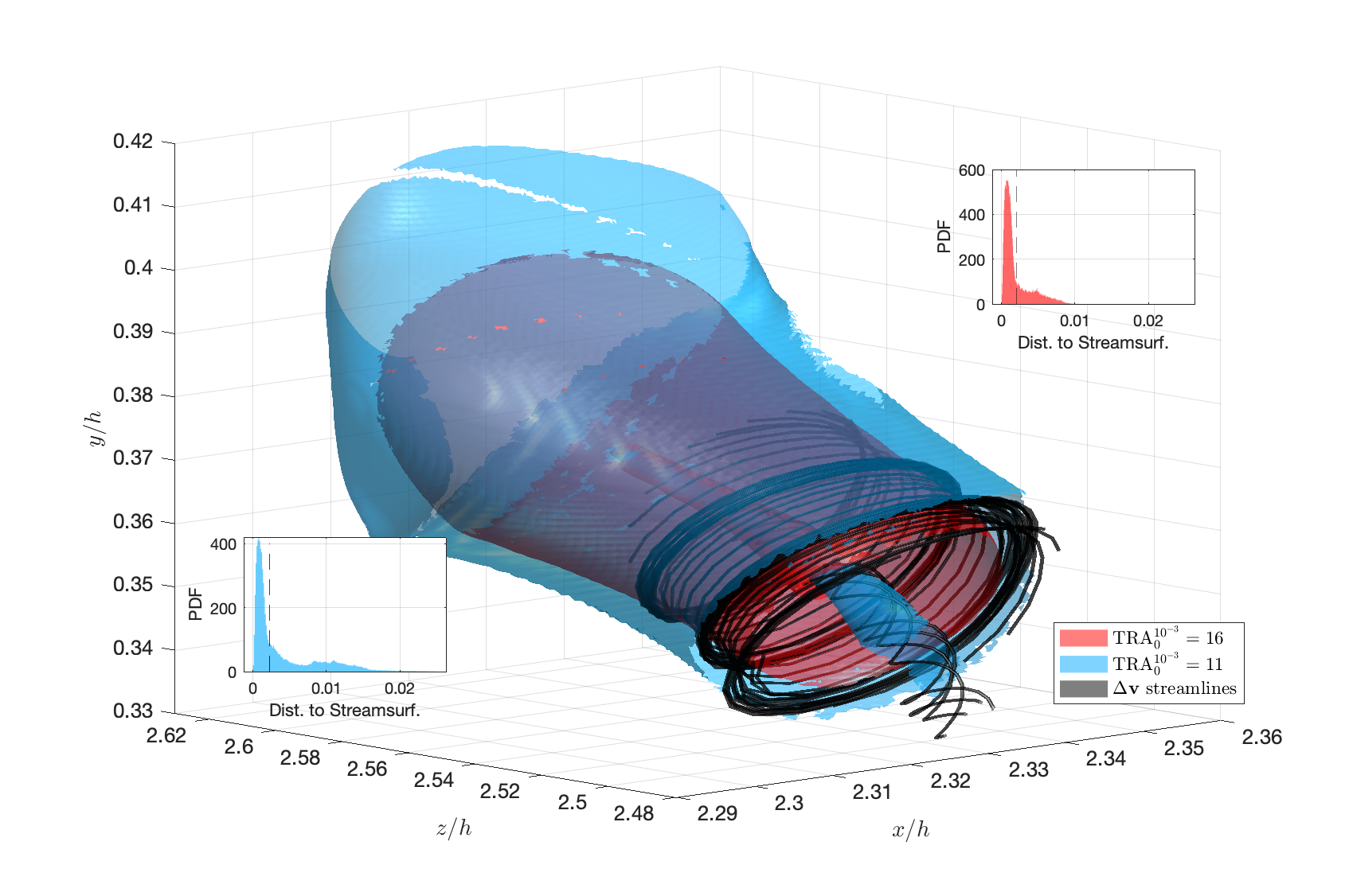
Figure 5: TRA isosurfaces as approximations to the momentum transport barriers shown in Figure 4. Blue and red surfaces correspond with two distinct $\mathrm{TRA}_{0}^{10^{-3}}$ values. Shown in black are a subset of streamlines initiated on the $\mathrm{TRA}_{0}^{10^{-3}}=16$ contour on the $z=2.55$ plane. Inset are probability distribution functions of the minimum distance of unfiltered surface points to streamlines initialized on TRA contours at $z=2.55$.

Starting with the vortex identified by the blue 2D convex contour in Figure 4, multiple concentric 3D TRA shells can be seen in Figure 5. The outer and inner blue shells correspond with $\mathrm{TRA}_{0}^{10^{-3}}=11$ level sets, and the two red shells correspond to a higher rotation rate, the $\mathrm{TRA}_{0}^{10^{-3}}=16$ level set. Probability distribution functions of the distance between each isosurface and the barrier field streamlines generated from their intersection with the $z=2.55h$ plane is shown inset in Figure 5. As is typical for all vortices we have investigated, there is a clear probability density function (PDF) peak close to zero that can be automatically isolated for both isosurfaces with a variety of algorithms, including inflection points or kernel density estimation. These values correspond with points on the TRA level surface that closely approximate the momentum-blocking invariant manifolds in Figure 4. Once points with streamsurface-distances outside this peak are removed from the visualization, the separation between each vortex shell is clearly visible. The selected distances of separation used in this visualization are shown in the inset PDFs as dashed vertical lines. The details of this process are also summarized in Algorithm 1.

To quantify how well outermost cylindrical TRA level surfaces, denoted $\mathcal{I}_{\mathrm{TRA}}$, approximate true momentum barriers, we calculate the normalized objective geometric flux $\Psi\left(\mathcal{I}_{\mathrm{TRA}}\right)$ defined in (10), which vanishes only on perfect barriers to momentum transport. For comparison, we also extract representative isosurfaces of $\lambda_{ci}$, $\lambda_{2}$ and $Q$, denoted by $\mathcal{I}_{\mathrm{\lambda_{ci}}}$, $\mathcal{I}_{\mathrm{\lambda_{2}}}$ and $\mathcal{I}_{\mathrm{Q}}$, in the same 3D fluid volume and calculate $\Psi$ on these surfaces as well. While there are various empirical values proposed for representative $\mathcal{I}_{\mathrm{\lambda_{ci}}}$, $\mathcal{I}_{\mathrm{\lambda_{2}}}$ and $\mathcal{I}_{\mathrm{Q}}$ isosurfaces (see, e.g., Jeong & Hussain (1995); Zhou et al. (1999); Ganapathisubramani et al. (2006); Gao et al. (2011); Dong & Tian (2020)), we initially generate surfaces that correspond with their originally argued value, dividing strain-dominated and rotation-dominated regions. This value is zero for all velocity-gradient-based metrics (see Hunt et al., 1988; Jeong & Hussain, 1995; Zhou et al., 1999).

The isosurfaces generated for each scalar metric are displayed in Figure 6.

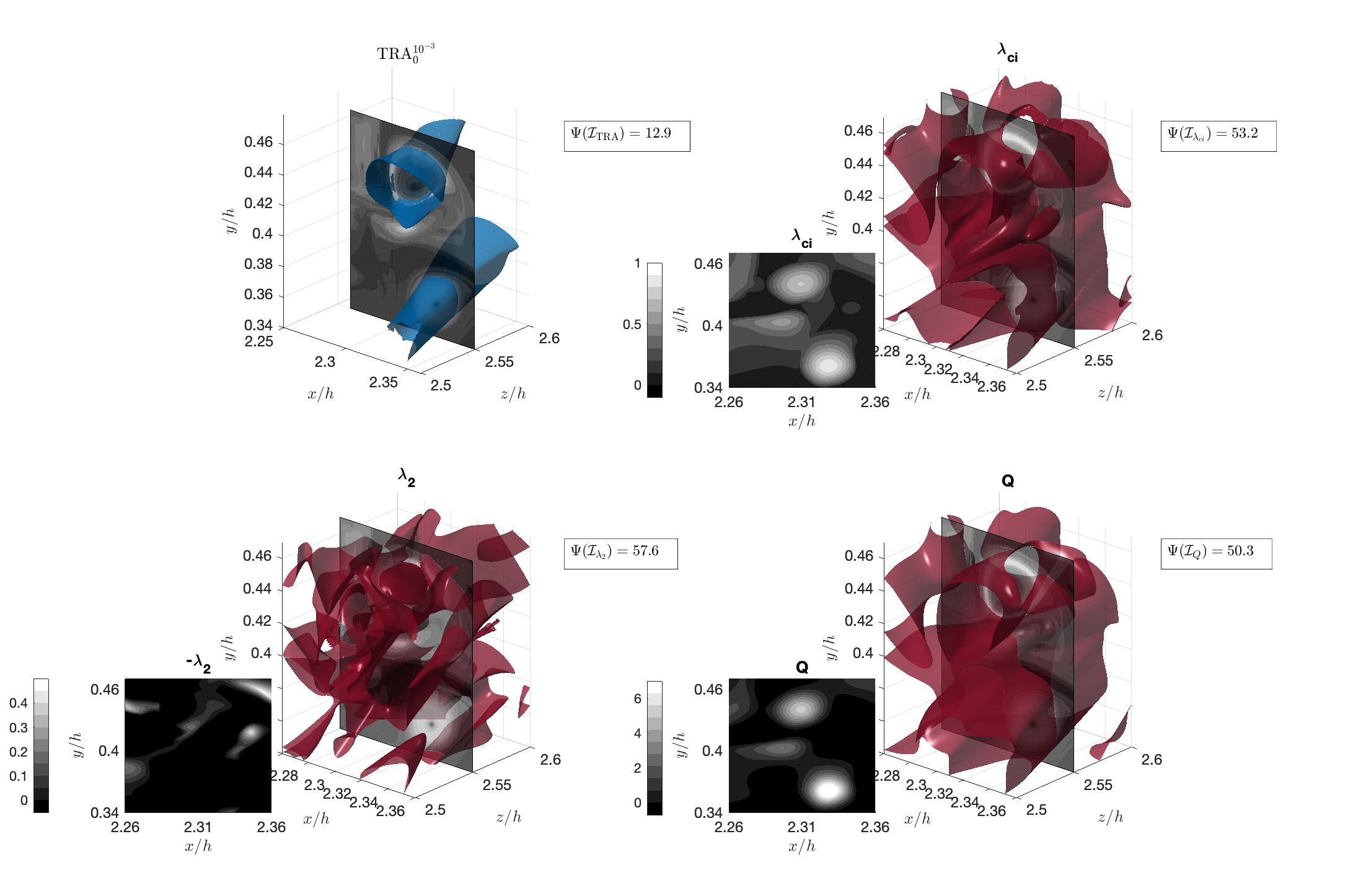
Figure 6: Comparison of area-normalized objective momentum flux values for vortex boundaries identified from different vortex identification methods.

As common practice, the swirling strength $\lambda_{ci}$ has been normalized by its maximum value in the volume of interest. Each isosurface is shown as it intersects the $z=2.55h$ plane colored by $\mathrm{TRA}_{0}^{10^{-3}}$. For the three velocity-gradient-based diagnostics, the corresponding diagnostic field on $z=2.55h$ is shown inset next to the volumes. The surface-area-normalized momentum flux across each isosurface is also noted to the right of each respective volume.

In the $z=2.55h$ insets, $\lambda_{ci}$, $\lambda_{2}$ and $Q$ values all show some indication of the presence of the upper vortex from the TRA field, though evidence of the lower vortex is not present in $\lambda_{2}$. This suggest the presence of our physical momentum barriers may have influenced these scalar fields, but the metrics are ineffective at predicting where the transport barriers lie. Even as simplified approximations of true linear-momentum barriers, TRA isosurfaces are still quite effective momentum transport barriers. Indeed, $\Psi(\mathcal{I}_{\mathrm{TRA}})$ is only $24\%$ of $\Psi(\mathcal{I}_{\mathrm{\lambda_{ci}}})$, $22\%$ of $\Psi(\mathcal{I}_{\mathrm{\lambda_{2}}})$ and $26\%$ of $\Psi(\mathcal{I}_{\mathrm{Q}})$. Recall that $\Psi=0$ for the invariant manifolds in Figure 4 that $\mathcal{I}_{\mathrm{TRA}}$ is approximating here.

We have found that with increased numerical accuracy in our barrier field integrations, TRA calculations improved and resulted in a further decrease in $\Psi(\mathcal{I}_{\mathrm{TRA}})$. This indicates one can more closely approximate the true momentum transport barriers with more computational expense when a particular region of interest is identified. We have not found analogous numerical improvements in flux reduction upon refining the spatial differentiation or resolution of the velocity-gradient-based methods. Overall, we find that the classic vortex diagnostics we have tested do not provide a clear indication of a pair of 3D vortices when one directly implements the criteria arising from their theoretical derivations. Rather, one must hand pick values to obtain a vortical feature in two or three dimensions as noted by Dubief & Delcayre (2000); Dong & Tian (2020). This is problematic in turbulent flows where there is no ground-truth of structure topology against which one can validate their hypothesized threshold values.

To accommodate the wide range of empirical or heuristic thresholds used in the literature, we have also performed the same flux calculations for $\lambda_{ci}$, $\lambda_{2}$ and $Q$-isosurfaces for a range of values that includes and exceeds available suggestions found in the literature. The resulting fluxes are displayed in Figure 7.

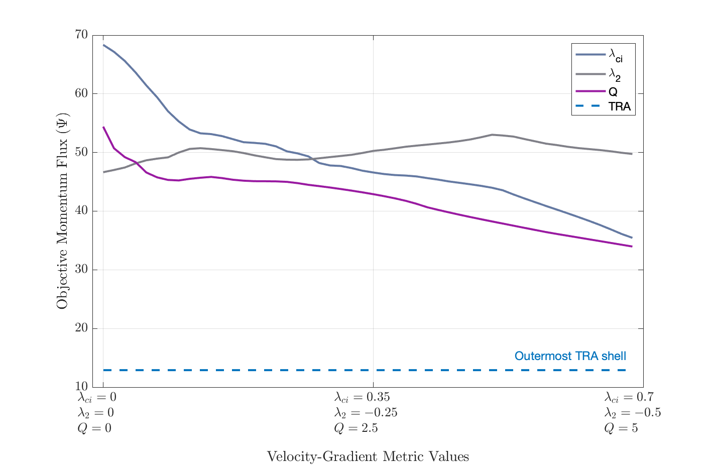
Figure 7: Comparison of momentum flux through $\mathcal{I}_{\mathrm{TRA}}$ and through structure boundaries defined by a wide range of isosurface values for the $\lambda_{ci}$, $\lambda_{2}$ and $Q$ metrics.

Note that $\mathcal{I}_{\mathrm{TRA}}$ in blue continues to outperform all other diagnostics over the whole range of empirical threshold values for the latter diagnostics.

In Figure 8, we verify the surface tangency of arbitrary-valued $\mathrm{TRA}$ level-surfaces with invariant manifolds.

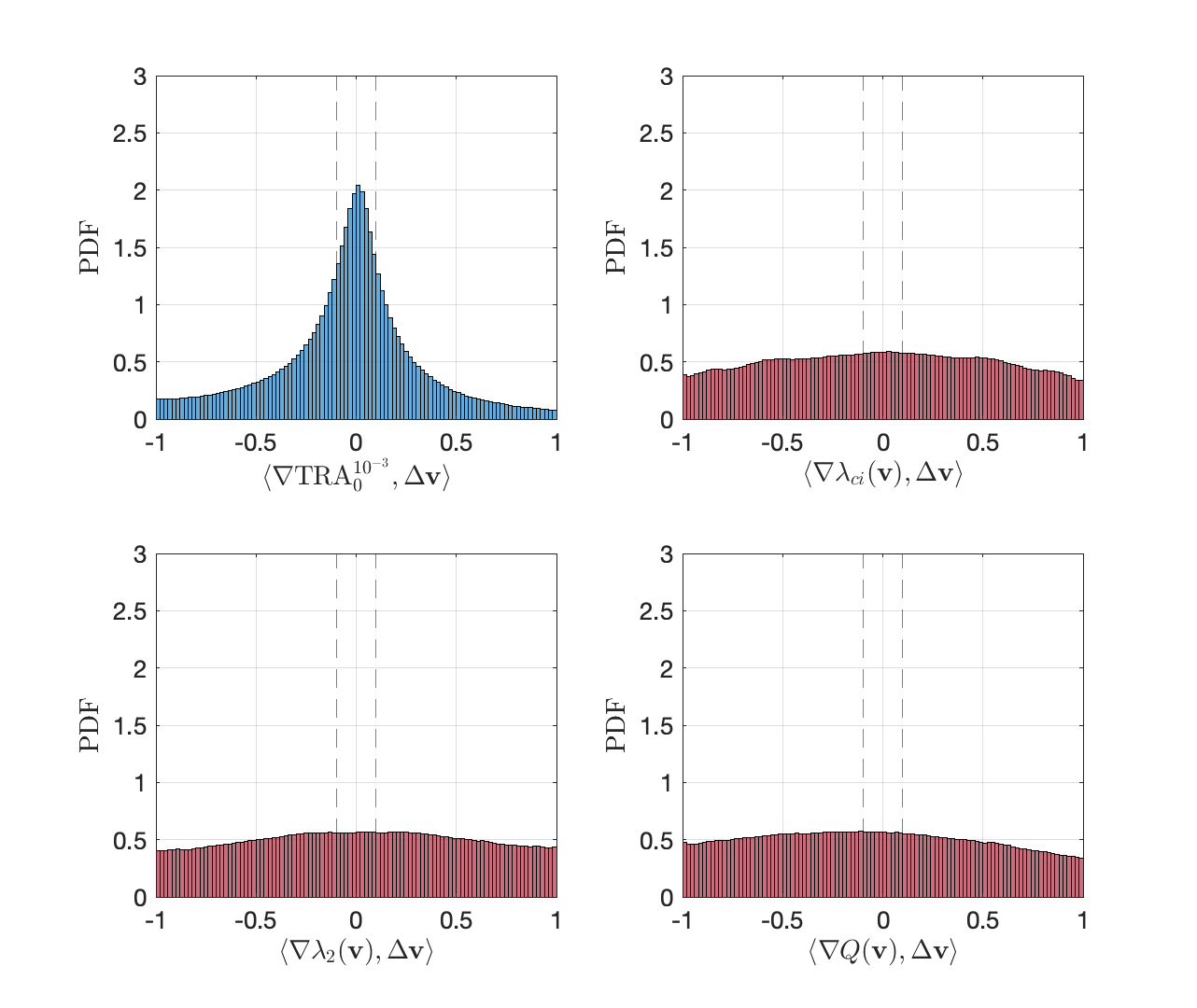
Figure 8: Probability distributions of the normalized inner product of momentum barrier field vectors and isosurface normals for TRA and the three standard velocity-gradient-based diagnostics for a 3D rectangular volume of fluid containing the vortices in Figure 6. The clear singular peak around 0 in the TRA PDF indicates a strong agreement between TRA surfaces and the underlying momentum transport blocking interfaces for both elliptic and hyperbolic surfaces. Similar behavior does not exist for the other three diagnostics. A $\pm 5^{\circ}$ difference between surface tangents and barrier vectors is delimited by dashed lines.

If isosurfaces of a given scalar field were exact streamsurfaces of the barrier equation, then their normals (i.e., the gradient of that scalar field) would be perpendicular to $\Delta\mathbf{v}$. Each subplot of Figure 8 shows the probability distribution of inner products of normalized scalar field gradient vectors with the normalized barrier field, $\Delta\mathbf{v}/\left|\Delta\mathbf{v}\right|$, over the entire 3D volume containing our vortices ($[2.26,2.36]\times[0.34,0.37]\times[2.5,2.6]$). These are precisely distributions of the signed integrands of the numerator in (11). Vertical dashed lines mark a $\pm 5^{\circ}$ deviation from perfect agreement between momentum barriers and barriers generated by each diagnostic level set. Notably, there is a clear peak around 0 for $\boldsymbol{\nabla}\mathrm{TRA}_{0}^{10^{-3}}$ , while a nearly uniform (random) distribution can be seen for angles between barrier field vectors and velocity-gradient-based isosurface normals.

As the linear-momentum barrier vector field $\Delta\mathbf{v}$ is objective, extracting the classic $\lambda_{ci}$, $\lambda_{2}$ and $Q$ level surfaces from the $\Delta\mathbf{v}$ field would also be an objective procedure, unlike extracting these level surfaces from the velocity field $\mathbf{v}$, as originally intended for these diagnostics. To see if such an objectivization would benefit these criteria, we have carried out the same statistical structure-tangency analysis with the $\lambda_{ci}$, $\lambda_{2}$ and $Q$ metrics now applied to the barrier field $\Delta\mathbf{v}$. While the resulting PDFs in Figure 9 now show a moderate rise near zero for each classic vortex diagnostic, TRA level-sets still outperform the other diagnostics in their ability to block the viscous transport of momentum. This suggests that TRA level sets are overall close approximations to the perfect momentum barriers formed by invariant manifolds of the barrier equation (9).

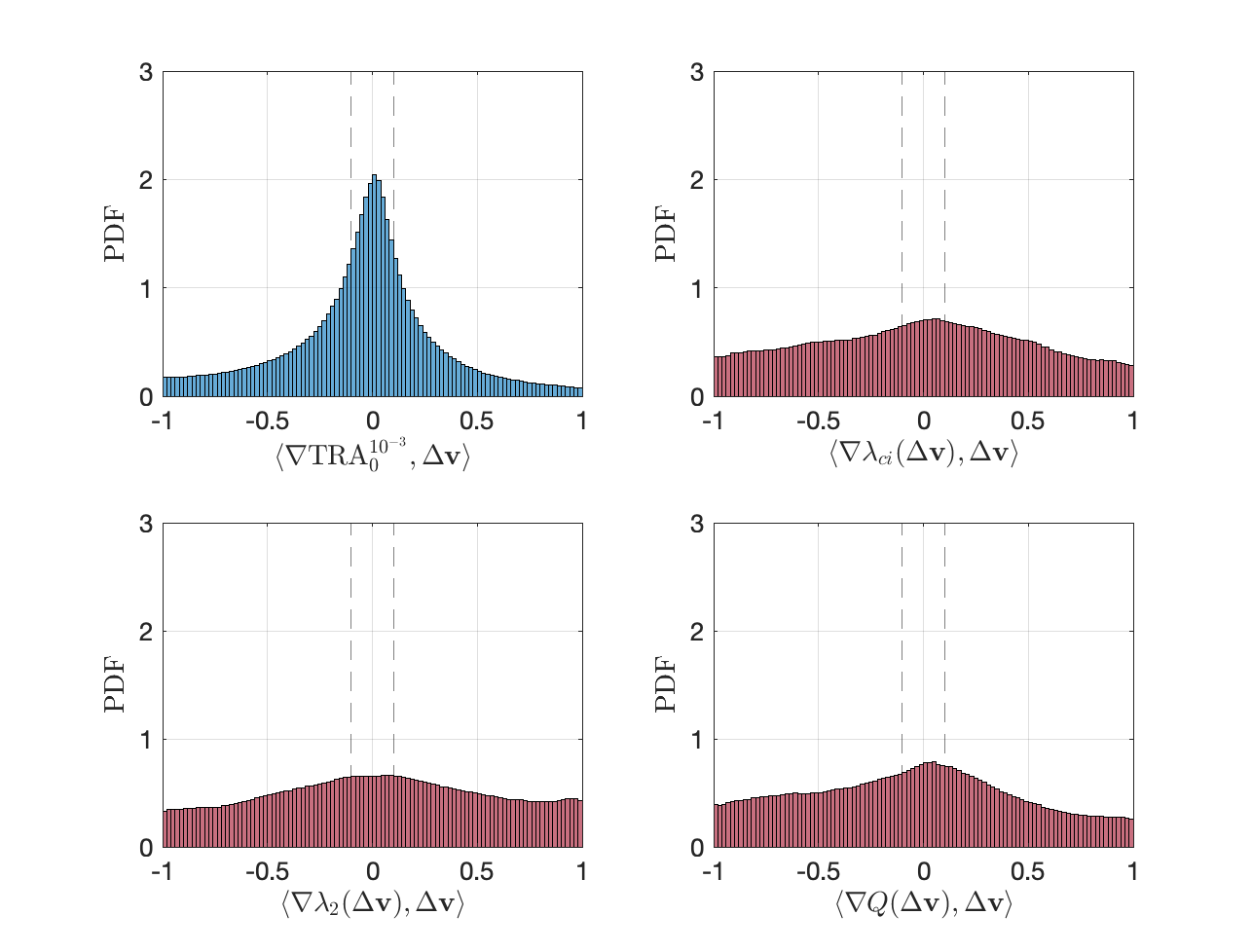
Figure 9: Same as Fig. 8, but with the $\lambda_{ci}$, $\lambda_{2}$ and $Q$ metrics computed for the barrier equation (9).

3.3 Momentum transport barrier interfaces

We have, so far, used level surfaces of the TRA field for the approximate visualization of vortices with a perfect instantaneous momentum-trapping property. We can also use the TSE field to interrogate the momentum barrier equation more globally in order to locate momentum-blocking interfaces between more and less turbulent areas of the flow. This can be achieved by constructing streamsurfaces of the barrier equation that partition the flow into wall-parallel domains with boundaries that span the channel in the wall-parallel directions. We use TSE fields to aid in this interface identification as their level surfaces separate regions of distinct degrees of stretching in a manner analogous to hyperbolic invariant manifolds. We use the single smoothest interface as this provides the barrier with the least folding. As shown in Figure 10, there are multiple spanning TSE interfaces in a given domain. These interfaces contour around vortices that compose large scale motions. After analyzing 100 temporal frames of TSE fields, we find that using the average straightest contours allows us to connect the outermost contour around these vortices. This selection can be modified for other flow-specific criteria, and a statistical analysis of all candidate TSE interfaces is conducted in Section 3.4.

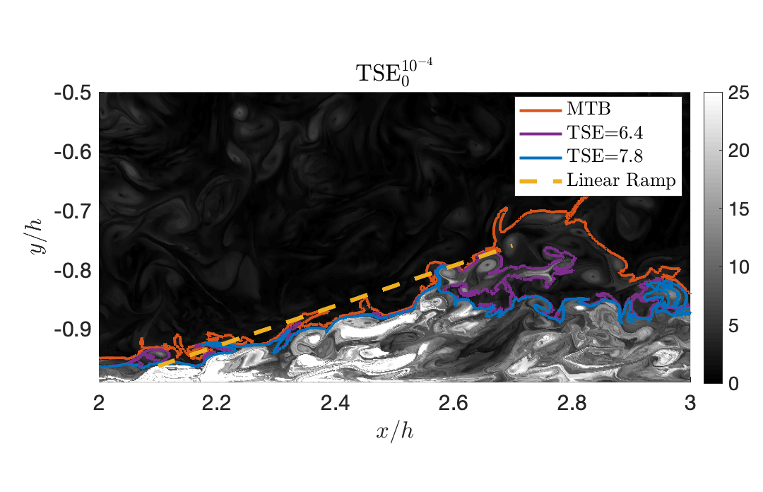
Figure 10: TSE contours with the smoothest contour selected as an MTB. A linear ramp identified by a linear-fitting search is also drawn in. Note that the MTB is more effective at contouring around the outside of vortices whereas the other two TSE contours filament and penetrate the interiors of vortices.

We now describe a simple, automated algorithm for identifying such objective momentum transport barriers (MTB) as a physics-based alternative to the currently used TNTI or UMZ interface identification processes (Adrian et al., 2000b; Da Silva et al., 2014; De Silva et al., 2015). This algorithm is also sketched in Algorithm 2. As with our vortex identification, when using the trajectory decorrelation time for TSE calculations, we only use one free parameter in our MTB algorithm: the choice of spatial resolution, which is approximately 1 viscous length in all directions. This ultimately controls the level of detail in the MTB interfaces and their momentum-blocking ability. In contrast to common TNTI or UMZ level-surface approaches, we can progressively improve our momentum-barrier identifications by calculating TSE at progressively finer resolutions beyond the underlying velocity grid. This improves surface triangulations and enhances tangency with invariant manifolds in the barrier field (9).

	Algorithm 2: Extracting MTB
1	For a co-dimension 0 domain of interest $U\subset\mathbb{R}^{3}$, select a grid of initial conditions $\mathbf{x}_{0}\in U$.
2	Determine the optimal barrier time $\epsilon_{0}$ using TSE calculations (instead of TRA) in Steps 2-4 in the vortex core extraction algorithm.
3	For each streamwise-wall-normal hyperplane $V_{z}$ that intersects $U$, extract iso-contours in $V_{z}$ for the range of TSE values present in $V_{z}$. Record only the contours $\left\{\gamma_{j}\right\}$ that span the full streamwise width of the domain.
4	Refine $\left\{\gamma_{j}\right\}$ to corresponding TSE values with contours that span the domain for every $V_{z}$.
5	Select the TSE value such that the corresponding $\gamma_{j}$ span each $V_{z}$ with minimal length.
6	Extract the connected TSE isosurface corresponding to this TSE value that intersects the $\gamma_{j}$ of interest.

We begin this algorithm by calculating the TSE for the active barrier equation (9) on a 3D domain of interest. Here we use the decorrelation time as determined for the wall-proximal (outer) quarter of the channel ($|y|\geq 0.75$) in an effort to visualize the most turbulent and complex momentum blocking structures ($s_{N}=10^{-4}$) emanating from the wall. Through a sensitivity analysis, we found MTB identification to be consistent over six orders of magnitude of $s_{N}$, but the visual clarity of near-wall structures begins to deteriorate away from our chosen $s_{N}$. Note that these six orders of magnitude relate to the integration time of a trajectory in the barrier field equations, and not to a physical spatial or temporal dimension. For example, a longer integration time may allow initially adjacent particles to separate to a larger degree, or for a trajectory in a vortex core to circulate more, thus allowing for more distinct TSE and TRA contours, but not necessarily a different size of spatial features. As well, the $s_{N}=0$ limit exists, providing an estimate of the structures detailed here. The decorrelation time for visualization close to the wall is shorter than the value $s_{N}=10^{-3}$ calculated for our focus on vortices near the center of the channel as the magnitude of the $\Delta\mathbf{v}$ is much greater near the wall and a shorter integration time is sufficient to obtain the same degree of detail.

To reduce the computational burden of finding the smoothest domain-spanning interface, we first perform a series of 2D approximations. We select a set of $n\geq 1$ streamwise-wall-normal planes and identify the shortest TSE contour in each plane that divides the plane into a lower (wall-adjacent) and upper (central) region. For example, see the candidate spanning contours at $\mathrm{TSE}=3.11$ for multiple $z$ planes in the top row of Figure 11. Each such shortest, in-plane contour has a corresponding TSE value whose corresponding 2D TSE level surface is a candidate for an MTB interface. Of these candidate surfaces, we finally select the 2D TSE level surface whose intersection curves with the $n$ streamwise-wall-normal planes have the lowest maximum length. This procedure, therefore, yields the MTB interface as the TSE level surface that divides the flow roughly into parallel near-wall and mean-flow regions while maintaining as low a curvature as possible. The corresponding lower half-channel MTB determined from this algorithm can be see in the lower plot of Figure 11. The boundaries of the three upper planes of contour investigation are drawn in black. More involved algorithms targeting the same objective can certainly be devised but will likely come with increased computational cost.

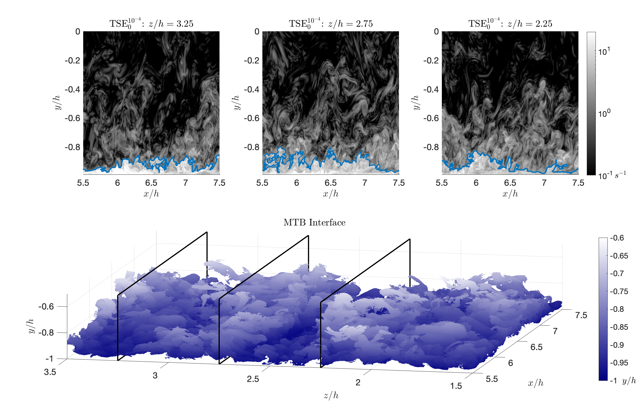
Figure 11: Top: Process of selecting the TSE contour that spans a domain of interest most efficiently among many adjacent 2D slices. Bottom: Corresponding TSE-derived momentum transport barrier (MTB) colored by y-values.

The MTB interface in Figure 11 is a complex structure that reveals connections of multiple vortices as they collect and migrate from the channel wall to the less turbulent center of the channel. The MTB has been shaded by the distance from the lower channel wall to help illuminate heterogeneity in the wall-normal extent of this MTB. Qualitatively familiar material features from smoke and dye experiments can be seen in this objective barrier. The organization of characteristic interface eddies documented by Falco (1977) and Head & Bandyopadhyay (1981) are evident along the MTB as well as the large scale streamwise streaky structures of Kline et al. (1967), with a spanwise spacing of approximately $0.75h$. There is also a striking similarity to scalar concentrations visualized in jet-driven TNTI (e.g. Westerweel et al., 2009)

The MTB interface obtained in this fashion approximates the flattest invariant manifold of the barrier equation that divides the flow into two disjoint quasi-wall-parallel layers with minimal diffusive momentum transport between them. The low-curvature requirement in the construction of this interface forces it to avoid highly turbulent regions and effectively connect outer regions of the momentum-trapping vortices that we have already discussed.

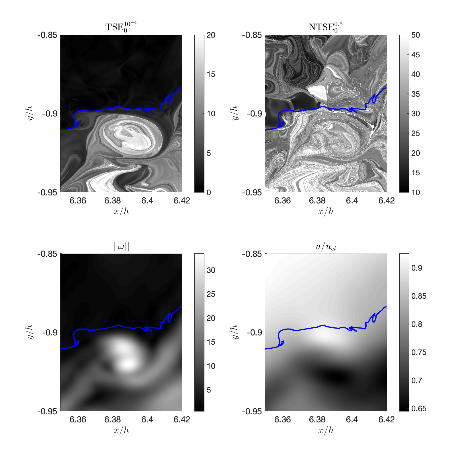
Figure 12: CW from the top left: The TSE field, the NTSE field for the unit barrier field, the streamwise velocity $u$ normalized by the centerline velocity $u_{cl}$, and the vorticity norm $\left\|\boldsymbol{\omega}\right\|$. The MTB interface is superimposed in all plots as a blue curve. All image data was computed and displayed at the same spatial resolution.

To illustrate this behavior, in Figure 12 we focus on a small subdomain of Figure 11 and compare our interface with two commonly used UMZ and TNTI identification diagnostics, vorticity and normalized streamwise velocity. While high-shear regions have been associated with UMZ interfaces (Hunt & Durbin, 1999; Adrian et al., 2000b), and have been used to help separate UMZs (Eisma et al., 2015), high-shear zones do not typically span the entire domain or provide a complete zonal separation of the flow. We thus conduct our comparison of domain-separating MTBs with other level-sets that span the domain. We also include in this comparison the NTSE field.

The top-left panel in Figure 12 shows TSE values calculated for initial conditions on the $z=2.75h$ plane with the interface drawn in blue. The interface effectively contours around the outside of a strongly stretching spiral feature and separates the flow into a less turbulent and more turbulent region. The NTSE field in the top-right panel reveals many of the same structures tangent to the MTB with additional weaker features aligned above the interface. Slight differences between contours in TSE and NTSE fields on the edge of the domain can be attributed to fixed time step integration effects.

The bottom-right panel shows the streamwise velocity, a scalar field whose contours are broadly used for extraction of uniform momentum zones in wall turbulence (e.g. Adrian et al., 2000b; Kwon et al., 2014; De Silva et al., 2015). Following the procedure of Kwon et al. (2014), we have normalized the velocities by the channel centerline velocity. We note that the predominant gradient in the velocity field follows approximately through the center of the vortical feature, and the velocity contours are parallel with the MTB in only a small region of the domain. We will further explore the differences between UMZ interfaces MTB interfaces below.

Lastly, the bottom-left panel of Figure 12 shows the vorticity norm in the same domain, a diagnostic commonly used in TNTI identification (see Holzner et al., 2006; Da Silva et al., 2014). This plot provides a similar but simpler picture of the flow dynamics in comparison with TSE, but the details do not indicate exactly where an interface should be drawn. There is no localized shear-driven vorticity peak along the turbulent interface, as is sometimes possible at the TNTI (Da Silva et al., 2014). As well, the change in vorticity is quite gradual, not giving a clear jump in the vorticity PDF as is often used to separate rotational and irrotational flow fields. For these reasons, vorticity is not commonly used for internal interface diagnostics, but is included here as it does provide a closer comparison with momentum barrier field behavior than the streamwise velocity (UMZ) visualization. As well, much of UMZ theory relies on an analogy with jumps across turbulent/non-turbulent interfaces.

The ability of the TSE field to identify divergent behavior of barrier streamlines and appropriately locate the MTB is illustrated in Figure 13. Here, we expand our focus from Figure 12 to a narrow subsection of the channel. The left column shows the local geometry of the MTB (blue) and UMZ (red) interfaces near the $z=2.75$ plane. The right column shows a zoomed in view of the interfaces in the domain of Figure 12 and the nearby trajectories of the barrier equation (9).

Trajectories are shaded by their TSE values. For the MTB interface, there is an obvious separation of minimally-stretching black trajectories in a less turbulent region above the blue interface and the multiple spiraling grey and white vortices below the interface. The MTB is also tangent to the barrier field streamlines, indicating the correct orientation with respect to the momentum barrier streamsurfaces. This is further confirmed in the inner-product probability distribution inset for the MTB on the left. Similar to the findings for TRA level-surfaces around vortices in Figure 8, the geometry of TSE level-surface interfaces is largely tangent to perfectly computed zero-flux linear momentum barriers.

The bottom-left panel of Figure 13 shows the universal $u/u_{cl}=0.95$ “quiescent core” UMZ interface calculated over the $1.2h$ streamwise extent, as suggested by Kwon et al. (2014). The MTB and UMZ interfaces differ greatly, but the UMZ interface does hint at being influenced by the TSE contours on the right side of the domain. This can be see in the inner-product PDF on the left with one such highlighted example shown in the bottom-right panel. The tangency PDF for the UMZ shows a slight peak around zero corresponding to near parallel points on the right side of the domain. Barrier field streamlines around a vortex feature, however, are seen to be perpendicular to the UMZ interface, thus maximizing transport. This is in direct contrast with our automated MTB interface algorithm that has clearly succeeded in approximating a repelling (and hence structurally stable) invariant manifold of the incompressible barrier equation. Of note, the UMZ interface transects the vortex core, as also seen by velocity contours in Figure 12. The UMZ interface is clearly not an organizing structure that blocks momentum transport, but these TSE fields and MTB may begin to give insight into the physical origins of the commonly seen statistical signatures that have supported the ubiquitous use of velocity isosurfaces.

While TSE level surfaces that span the domain at the height of the UMZ do exist, the nearby TSE structures contour and fold around many hyperbolic and elliptic barriers (such as those seen in Figure (2)) and do not provide a clear interface between distinct wall-parallel flow zones. We suspect that, in the neighborhood of the quiescent core interface, a simple quasi-planar structure that blocks wall-transverse momentum flux may not actually exist as the elliptic and hyperbolic barrier field manifolds are less densely concentrated. The transverse intersections of velocity level surfaces with invariant manifolds of (9) in the PDF of Figure 13 suggest any possible correlations between velocity level surfaces and true momentum barriers are insignificant for predictive ability.

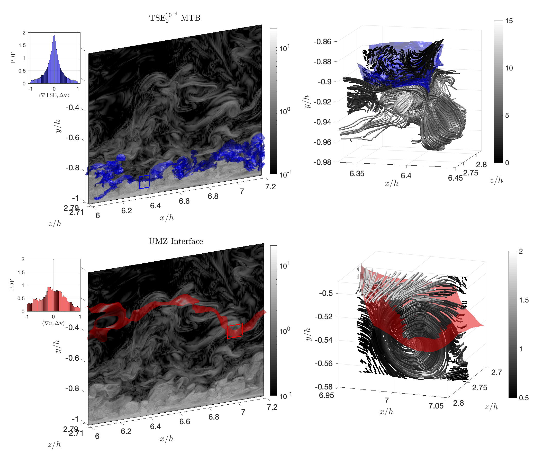
Figure 13: Top Left: TSE field and MTB interface. Bottom Left: TSE field and UMZ interface. Right: Corresponding interfaces and linear momentum barrier field trajectories colored by TSE. Inset in each plot are the corresponding PDFs of surface normal innerproducts with the barrier field indicating improved momentum transport limiting abilities of the MTB.

To assess this relationship more broadly, we compare the momentum transport through a range of UMZ interfaces and the MTB in Figure 14. The right panel shows the same TSE field for the $z=2.75h$ plane as in Figure 12 with overlaid streamwise velocity contours. As there are numerous approaches to extracting the best high-shear streamwise velocity isosurface for UMZ identification (see, e.g. De Silva et al., 2015; Fan et al., 2019), we directly compare our MTB with a range of simply connected velocity level surfaces from the near-wall region well into the channel core. The top left panel shows the geometric diffusive flux across this range of interfaces in red, and our MTB flux in blue. The gray shading indicates the $u/u_{cl}$ isosurfaces closest to the MTB in the domain. As with the non-objective diagnostics in Section 3.2, these velocity isosurfaces exhibit around four times the flux as our nearby objective MTB.

As we increase the velocity of the UMZ interface, we also move away from the wall and into a region with smaller $\Delta\mathbf{v}$ vectors. While we have seen that the quiescent core UMZ interface is largely transverse to momentum transport barriers, its diffusive momentum flux is smaller than for our MTB. We believe this is due to its location in a region with less turbulence and less flux, and not an ability to limit momentum transport. We thus calculate the normalized geometric flux (tangency measure) $\Psi_{N}$ from (11). In the middle panel, we present $\Psi_{N}$ for the same UMZ candidates. This shows the clear advantage of identifying internal momentum blocking interfaces with the MTB approach over any streamwise velocity isosurface. Triangles in the two flux plots mark several velocity isosurfaces of interest: the highest flux (0.63), the UMZ closest to the MTB (0.76), the trough between the two PDF peaks (0.88), and the quiescent core UMZ of Kwon et al. (2014) (0.95). The intersection of these four $u/u_{cl}$ isosurfaces with the $z=2.75h$ plane are drawn in the right panel.

UMZ theory suggests that momentum is organized into zonal-like structures inside of which there is relatively uniform momentum. These zones are separated by thin viscous shear layers that are often thought to concentrate spanwise vorticity (Meinhart & Adrian, 1995). Transport of momentum is concentrated to the viscous-inertial layers which separate the zones with the interfaces between them identifiable from streamwise velocity histograms. Whether in boundary layers or channel flows, UMZ interfaces have been defined as minima between peaks in the PDF for $u$, and correlated with high-shear. The bottom left panel of Figure 14 shows a PDF for the bottom half of the channel flow over the 3D domain of focus. These PDFs are known to be highly sensitive to the size and location of the domain of investigation but there is no consensus available on their use in 2D or 3D analysis (Fan et al., 2019). The level set values contoured in the right panel are marked on the PDF with dashed lines.

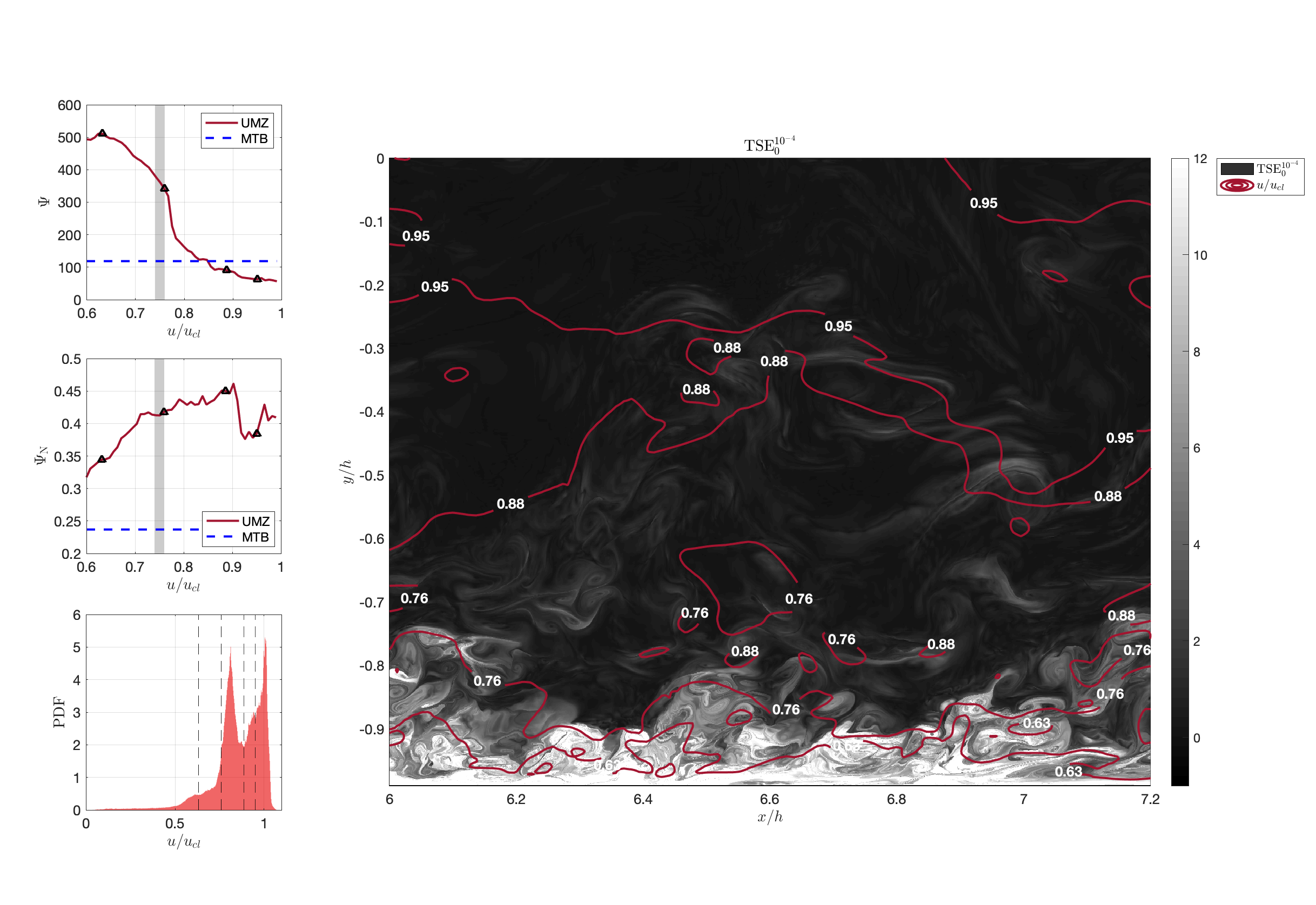
Figure 14: Top left: The surface-area normalized instantaneous viscous momentum flux $\Psi$ through streamwise velocity isosurfaces (UMZ interfaces). Middle left: $\Psi$ in unit barrier field for streamwise velocity isosurfaces. Bottom left: PDF of $u/u_{cl}$. Right: $u/u_{cl}$ contours (with their values indicated) superimposed in red over the TSE field in the $z=2.75$ plane.

It can be seen in Figure 14 that streamwise velocity contours interfaces with relatively low diffusive momentum flux do not correspond with momentum transport limiting structures. Indeed, all $u/u_{cl}$ interfaces travel transverse to multiple vortex cores (including that highlighted in Figure 13) and meander in and out of high stretching regions. In the $\Psi$ and $\Psi_{N}$ plots, we can see the surface derived from the minima between the two largest PDF peaks, $u/u_{cl}=0.88$, does not provide an even locally minimal momentum flux as has been suggested. The steady increase in $\Psi_{\mathrm{N}}$ and decrease in $\Psi$ for increasing $u$ shows the dominant influence of barrier field magnitude on $\Psi$ and a lack of momentum barrier tangency. In fact, the spanning velocity level surface with minimum momentum flux occurs at $u/u_{cl}=0.99$ which is well inside the less turbulent region of the flow. Of note, the quiescent core, $u/u_{cl}=0.95$, interface does indeed appear adjacent to the dominant channel core PDF peak, as suggested by Kwon et al. (2014). However, the $\Psi$ and $\Psi_{N}$ and plots shows no indication of significant momentum transport organizing structures and no indication which velocity isosurfaces exist inside or on the border of a momentum-organizing zonal-structure. That is, there is no evidence of shear-layers of localized vorticity that concentrate or minimize momentum transport between UMZs.

Each panel in Figure 15 shows the normalized inner product of respective isosurface normals with the momentum barrier field vector $\Delta\mathbf{v}$. As before, values around zero in the PDFs indicate an alignment of isosurfaces with true streamsurfaces of the momentum barrier equation. The top left panel shows a familiar peak around 0 for the MTB interface, confirming that the low momentum flux calculated across this interface is aided by its close alignment with a set of invariant manifolds of the barrier equation. There are impressively few isonormal vectors lying outside this peak even with the algorithm balancing strict coincidence invariance under the barrier equation with computational simplicity and moderate curvature.

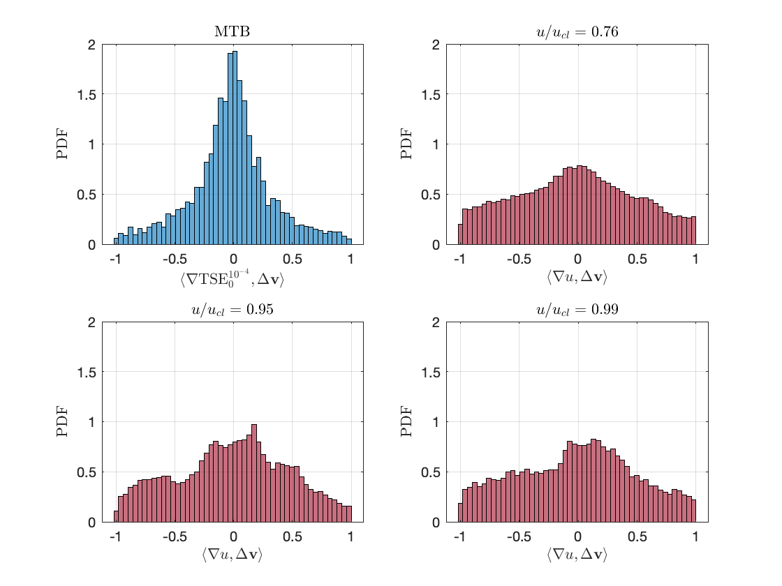
Figure 15: Probability distributions of the normalized inner product of the momentum barrier field vector, $\Delta\mathbf{v}$, and the isosurface normals for an MTB and UMZ interfaces. There remains a clear singular peak around 0 in the TSE PDF, indicating strong agreement between TSE surfaces and the underlying momentum transport blocking interfaces both for vortices and for the connecting regions between them. In contrast, there is significantly more momentum transport across UMZ interfaces.

In comparison, the PDF associated with the closest candidate UMZ interface to the MTB, $u/u_{cl}=0.76$, exhibits a subtle but much less pronounced peak around zero. Note that this surfaces experiences more than three times the momentum flux across it than the MTB interface. The other two velocity isosurfaces, including the quiescent cored interface, exhibit similar minor peaks around zero, with much more uniform and random alignment of surface normals when compared to the momentum barrier field vectors. This confirms our previous suspicion that flux is primarily minimized across this surface because of its location in a less turbulent region of the flow, and not because it behaves as a physically significant barrier. This is somewhat unsurprising as a simple wall-parallel plane in the neighborhood of the $u/u_{cl}=0.95$ level surface has a lower geometric objective momentum flux than the quiescent core boundary. However, for each contour $u/u_{cl}=0.76,$ 0.88, and 0.95, there are small sections of near tangency with the underlying momentum barriers. While velocity contours and momentum barriers are clearly not equivalent, this again suggests that method of momentum barrier identification is likely a beneficial avenue for investigating statistical signatures.

We have found the diffusive momentum transport blocking abilities of MTBs in the momentum barrier fields to be consistent in time frames spanning the entire DNS simulations. Focusing on $1.2h\times 0.5h\times 0.2h$ domains, we calculated TSE fields for 25 frames, generating more than 100 GB of TSE data. The PDF of normalized flux angles consistently follows similar behavior to that seen Figure 14, with an effective approximation to underlying invariant manifolds of the barrier equations.

3.4 Tracking features and temporal statistics

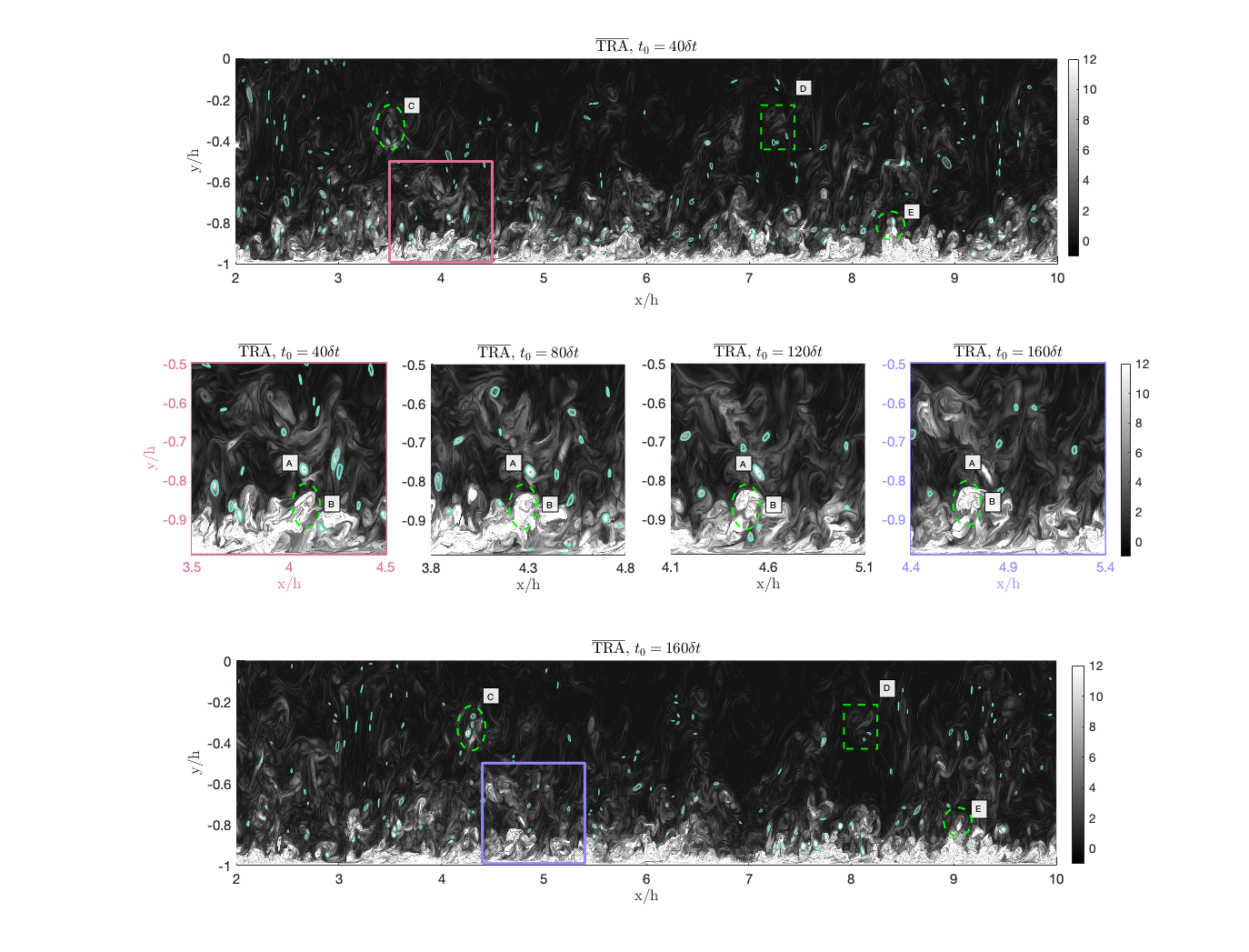
Figure 16: Subsequent $\mathrm{\overline{TRA}}$ fields in the x-z plane spanning 120 channel flow-through times. Multiple features that can be tracked throughout the frames have been identified, with a zoom section and intermediate frames shown in the middle plots. Vortex boundaries identified as the outermost closed $\mathrm{\overline{TRA}}$ contours are also drawn in, many of which can be tracked between frames.

The JHTDB Re=1000 channel flow spans 4,000 flow-through times ($\delta t$). We evaluated the frequency and recurrence of momentum-blocking vortex cores and MTBs in 100 frames with temporal spacing of $40\delta t$ spanning the entire available simulation time. Each frame is adjacent to the lower channel boundary, spanning $h\times 8h$ in the streamwise-wall-normal plane. This required analyzing 800 GB of velocity data, and resulted in 30 GB of TRA and TSE fields, which are available in the supplementary material, as is an animation of the time evolution of TSE frames.

A visual inspection of subsequent TRA and TSE fields reveals that many easily identifiable Eulerian features remain coherent during fluid advection and can be tracked from one frame to the next. One such example of this feature tracking is shown for the $z=3h$ plane in Figure 16. The top and bottom plots show TRA fields at $t_{0}=40\delta t$ and $t_{0}=160\delta t$, with the middle four frames tracking features in zoomed areas for intermediate timesteps. Some features of interest are labeled A-E; individual vortex cores following Algorithm 1 are highlighted in turquoise.

The vortex immediately to the right of the label A in the intermediate frames can be followed from $40\delta t$ to $160\delta t$, though the vortex eventually moves out of frame so that a circular contour is no longer extracted at $160\delta t$. The region labeled B is a cluster of tangled vortices near the top of a wall-connected bulge that is moving away from the wall. Because of the detail possible with TRA, individual components of B can be distinguished and followed between adjacent frames. From $40\delta t$ to $160\delta t$, vortices A and B remain identifiable while being advected nearly a full channel half-width down the channel.

In the wide-views at the top and bottom of the Figure, three additional features are identified and tracked. There are two vortex clusters, C and D, sitting approximately $0.7h$ from the wall in a much faster moving part of the channel. Vortex E is also tracked as the uppermost vortex on a bulge that has migrated approximately $0.75h$ down the channel. Note that the advection velocity of these five features is fairly consistent though their wall-normal locations vary by $0.6h$. The visual matching of these features was verified by advecting fluid particles in the DNS velocity field over this time window. While there was some minimal deformation of vortices over the period (not displayed), the advected structures and latter Eulerian detections indeed matched. This is promising for not only Eulerian studies of boundary layer structure evolution in great detail, but also the possible use of material momentum barriers from the Lagrangian theory of Haller et al. (2020). A video animation of the TRA fields in this plane spanning the entire DNS database be found in the supplementary movie.

By statistically analyzing the entire temporal extent of the channel flow simulation, we found similar behavior and characteristics for vortices and MTBs. We analyzed all TSE contours that spanned the $8h$ domain and found at least one such contour existed in each frame. The total number identified depends on the choice of the number of contour values to extract. At this Reynolds number, these contours were typically closely adjacent, as in Figure 10, though more distinct layering is likely at higher $Re$ as noted by De Silva et al. (2017). We include all TSE contours in our statistical analysis as candidate MTBs in light of potential advances in selection criteria and find this does not skew our statistics or introduce outliers. The median positive angle of each MTB was calculated and is displayed with respect to the median height of that momentum interface in the top-left panel of Figure 17. TSE contours follow the boundary of individual vortices and provide a measure of the incline angle of individual hairpins or typical eddies as a function of height. We find growth away from the wall in a similar fashion to existing attached eddy (hairpin vortex packet) models with angles ranging from $30^{\circ}$ up to $45^{\circ}$ further from the wall (Marusic, 2001).

Next, we measured the unit length per streamwise distance ($L_{s}/L_{x}$) of MTBs, similar to Chauhan et al. (2014) and De Silva et al. (2017). In the top-right plot of Figure 17, there is a clear increasing trend for barriers further from the wall. This agrees with the assessment in previous studies that, at greater distances from the wall, larger scale bulges and valleys contribute to greater $L_{s}/L_{x}$ (Townsend, 1976; Perry & Chong, 1982; Adrian et al., 2000b; De Silva et al., 2017). $L_{s}/L_{x}$ for our MTB exceeds the range of De Silva et al. (2017) ($<3$), but our mean, $\left<L_{s}/L_{x}\right>=5.4$, is much closer to that found by Chauhan et al. (2014) for the TNTI. This is likely attributed both to physical differences as well as the greater detail and meandering stream-surfaces found in $\Delta\mathbf{v}$ when compared to the underlying velocity grid (e.g. Figure 2).

By identifying the outermost closed and convex TRA contours, we found momentum vortex with have a mean diameter of $0.019h$. The PDF of this diameter distribution is shown in the bottom-right panel of Figure 17 with the mean marked as a dashed line. These vortex cores are smaller in diameter than the observed tracer eddies of Falco (1974, 1977), and slightly smaller than the $0.03-0.05\delta$ vortex heads identified by Adrian et al. (2000b). There are several possible reasons for this, the most probable being that the core vortical structure is smaller than its visible influence on the material (and velocity) field. We are restricting to closed and convex contours and thus eliminate the filamentation seen in smoke experiments.

Another commonly referenced statistic in the boundary layer literature is the inclination angle, $\alpha$, that the envelope of packets of vortices make with the wall, also known as the structure angle or ramp angle. This has been frequently measured by two-point correlations, with limited guidance for quantifying spatially-resolved structures beyond the Radon transform used by Hommema & Adrian (2003). We opt to measure the inclination angle of 0.6$h$-streamwise-length linear segments that fit our contours of interest with $\mathrm{RMS}<0.02$, the average diameter of our vortices. This length was chosen as it is less than the lower bound of the streamwise length of bulges reported in the literature, and approximately one half the streamwise extent necessary for converged channel flow UMZ statistics (Kwon et al., 2014). This provides sufficient streamwise range to find a good linear fit to a ramp without fitting to the small individual sub-components or the large scale motions. An example of a successful linear fitting is shown in Figure 10.

The average $\alpha$ value is found to be $8^{\circ}$ with the average ramp center approximately $0.18h$ away from the wall. There were approximately $75\%$ as many ramps identified as total number of MTBs. While these angles and heights are similar to the observations of Head & Bandyopadhyay (1981), and seminal UMZ work (see, e.g. Adrian et al., 2000b), there is significant scatter around these values as can be seen in the bottom-left of Figure 17. This suggest the linear fit method should be refined further in future momentum barrier investigations.

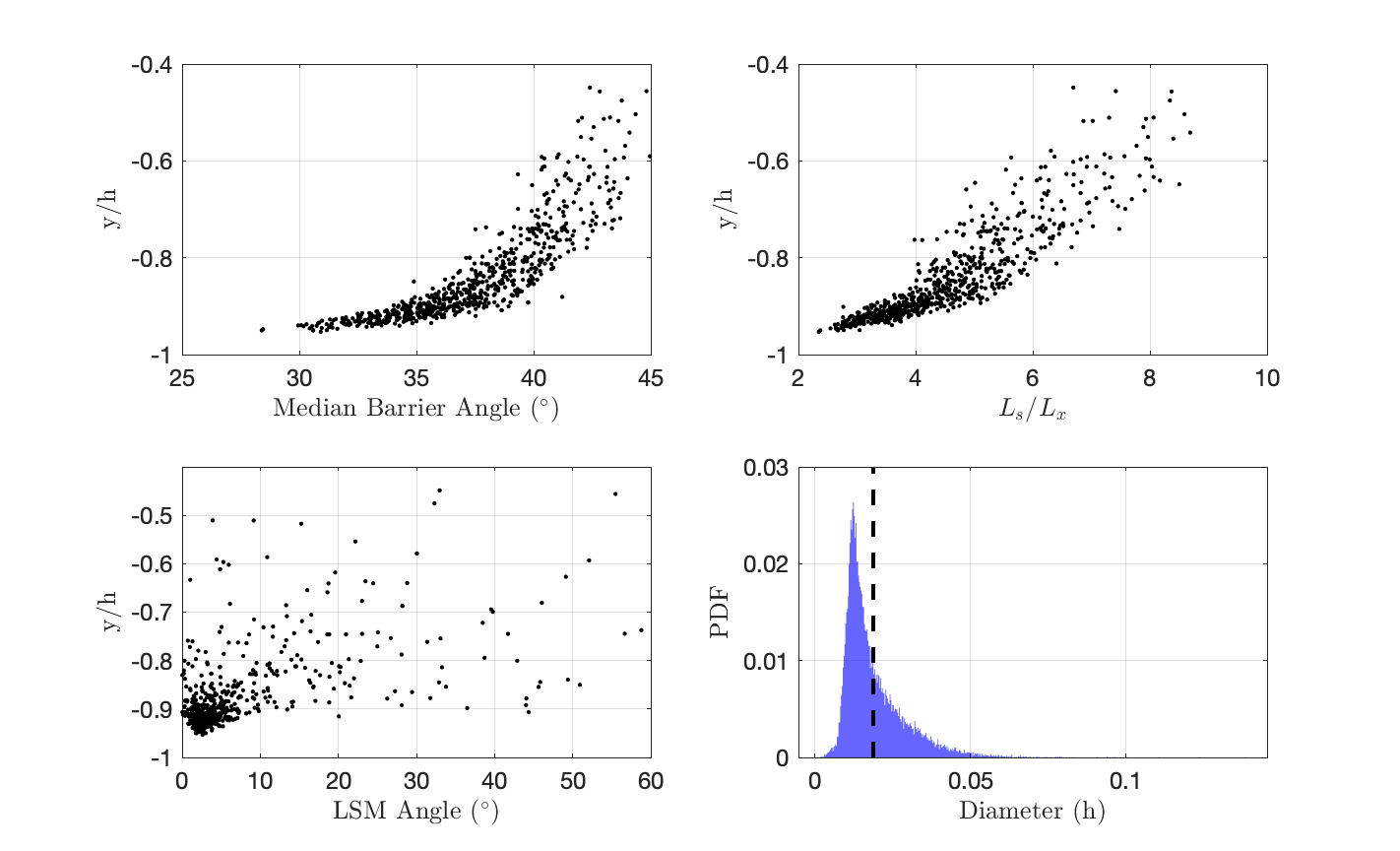
Figure 17: Interface angles and radii of vortex cores (heads) over in 3D frames spanning 4,000 flow-through times.

4 Conclusions

Using the objective notion of diffusive momentum flux through a material surface, we have developed an algorithm for locating frame-invariant instantaneous barriers to linear momentum transport in near-wall turbulence. This algorithm builds on the recent theory of active transport barriers (Haller et al., 2020), which identifies momentum transport barriers as structurally stable invariant manifolds (stream surfaces) of the incompressible steady barrier equation (9). Our algorithms extract these invariant manifolds directly and approximate them by level surfaces of recently developed coherent structure diagnostics, the trajectory rotation average (TRA) and trajectory stretching exponent (TSE) proposed by Haller et al. (2021). Other objective LCS diagnostics can also be used to identify invariant manifolds of (9), but TRA and TSE were used here due to their computational simplicity as single-trajectory-based diagnostic fields and their ability to designate clean boundaries. We also introduce the normalized NTRA and NTSE, which provide unprecedented detail for coherent structures, with equal fidelity in highly turbulent and less turbulent zones.

Our procedure targets both momentum-trapping vortices in the boundary layer and internal momentum-flux minimizing interfaces that locally define the flow into near-wall and far-from-wall layers. Specifically, vortex boundaries are identified as the outermost cylindrical level surfaces of the TRA field. This procedure is free from the empirical threshold values employed by classic, velocity-gradient-based vortex criteria which provide observer-dependent results. In addition, we find that while classic vortex identification diagnostics can suggest vortices in the neighborhood of these momentum-blocking vortices, this similarity is without predictive value and fails to generate surfaces that sufficiently block momentum transport. We believe that the underlying momentum-blocking structures are influencing the gradient-based diagnostics, but the classic diagnostics cannot be used as a proxy measure as they maintain no predictive physical (transport-limiting) value.

The same barrier field trajectory data can also be used to compute TSE fields and identify wall-parallel quasi-planar momentum transport barrier (MTB) interfaces that locally minimize the diffusive transport of momentum. With TRA and TSE fields, the diffusive linear momentum barrier vector field (9), therefore, links vortex diagnostics with internal fluid interfaces, as seen in tracer field observations, and are objective analogues of the broadly used but frame-dependent UMZ interfaces and TNTIs. We have found that MTB interfaces significantly outperform the classic UMZ interface approaches, in terms of their ability to block viscous momentum transport, regardless of the specific velocity chosen. The use of TSE calculations for the barrier equations eliminates sensitivities in UMZ analysis with respect to changes in the number of bins used in velocity histograms and variations in the size of the domain of analysis. In comparison, the only free parameter in our vortex and MTB algorithm is the spatial resolution of TSE fields, although this is simply a question of computational resources. Whereas increases in spatial resolution reduce momentum transport through vortex and MTB extractions, increases in the number of velocity histogram bins eventually lead to the disappearance of any UMZ peak or interface.

This first-principles approach of starting with an objective momentum flux provides universal diagnostics based on physics for future structure extraction techniques, the $\Psi$ and $\Psi_{N}$ fields. Furthermore, the objective nature of this work provides frame-indifferent structures that are experimentally verifiable (e.g. Eisma et al., 2021), unlike the predictions from non-objective criteria. The vortices and MTB identified are resilient under fluid advection, providing a new way in which to track the evolution of individual or clusters of structures. In this way, we hope to provide a common test to verify models and settle longstanding debates in fluids, such as the prevalence or importance of hairpin structures in the boundary layer (see, e.g., Marusic & Monty, 2019), and the role of inner versus outer layer motions.

Techniques for three-component PIV measurements are rapidly advancing (Raffel et al., 2018), and the momentum-transport barrier techniques examined here provide a new way to identify such barriers in an observer-independent fashion in the same flow volume as these data increase in ubiquity. For experimental flows in which volumes of 3D measurements are not available, there is also potential for developing symmetry arguments, such as those provided by Haller et al. (2020). These can, for instance, simplify the barrier vector field to fewer components for flows with strong anisotropy. Qualitative comparisons between structures in numerical simulations and tracer experiments may also provide insights by determining the roles of analogous features when experimental velocity measurements are unavailable.

Future research should investigate the role that parabolic invariant manifolds of the momentum barrier equation (9) play in near-wall turbulence as well. Haller et al. (2020) also derive a barrier equation for the transport of vorticity, which takes the form $\mathbf{x}^{\prime}=\Delta\boldsymbol{\omega}$. The streamsurfaces of the latter barrier equation generally differ from those of equation (9) and hence would highlight different internal interfaces in near-wall turbulence in a theory that seeks vorticity transport minimizing interfaces. Another extension of the present theory could use the Lagrangian active barriers introduced in Haller et al. (2020), which are material surfaces minimizing momentum or vorticity transport over a whole time interval rather than just instantaneously. Such material barriers should mimic the structures seen in the classic smoke experiments of Falco (1977) even more closely.

Appendix: Total Objective Momentum Flux

For the unsteady ABC flow

$$\mathbf{v}(\mathbf{x},t)=e^{-\nu t}\mathbf{v}^{0}\left(\mathbf{x}\right),\qquad\mathbf{v}^{0}\left(\mathbf{x}\right)=\left(\begin{array}[]{c}A\sin x_{3}+C\cos x_{2}\\ B\sin x_{1}+A\cos x_{3}\\ C\sin x_{2}+B\cos x_{1}\end{array}\right),$$ (16)

Theorem 7.5 of Haller et al. (2020) guarantees that the instantaneous barriers to diffusive momentum transport coincide with the structurally stable 2-D invariant manifolds of the flow generated by the steady velocity field $\mathbf{v}^{0}$, as well as the material and instantaneous barriers to vorticity transport. Specifically, the Eulerian barrier equation for momentum transport is

$$\mathbf{x}^{\prime}=\nu\rho\Delta\mathbf{v}=-\nu\rho k^{2}\alpha(t)\mathbf{v}^{0}(\mathbf{x}).$$

Note that

$$\mathbf{v}_{t}=-\nu\mathbf{v}^{0}\left(\mathbf{x}\right),\quad\nu\Delta\mathbf{v}=-\nu\mathbf{v}^{0}\left(\mathbf{x}\right),$$

where the second identity follows from the Beltrami property with $k=1$ in this case. Therefore, using the Navier–Stokes equations, we obtain

$$-\frac{1}{\rho}\boldsymbol{\nabla}p=\left(\boldsymbol{\nabla}\mathbf{v}\right)\mathbf{v} =\left(\begin{array}[]{ccc}0&-C\sin x_{2}&A\cos x_{3}\\ B\cos x_{1}&0&-A\sin x_{3}\\ -B\sin x_{1}&C\cos x_{2}&0\end{array}\right)\left(\begin{array}[]{c}A\sin x_{3}+C\cos x_{2}\\ B\sin x_{1}+A\cos x_{3}\\ C\sin x_{2}+B\cos x_{1}\end{array}\right)$$ (27)

$$=\left(\begin{array}[]{c}-BC\sin x_{1}\sin x_{2}+AB\cos x_{1}\cos x_{3}\\ BC\cos x_{1}\cos x_{2}-AC\sin x_{2}\sin x_{3}\\ -AB\sin x_{1}\sin x_{3}+AC\cos x_{2}\cos x_{3}\end{array}\right)$$

The pressure gradient, therefore, has a different magnitude and orientation relative to $\Delta\mathbf{v}=\mathbf{v}^{0}$ . This discrepancy can indeed be seen in Figure 18 where the FTLE field is calculated for $\Delta\mathbf{v}$ and (27).

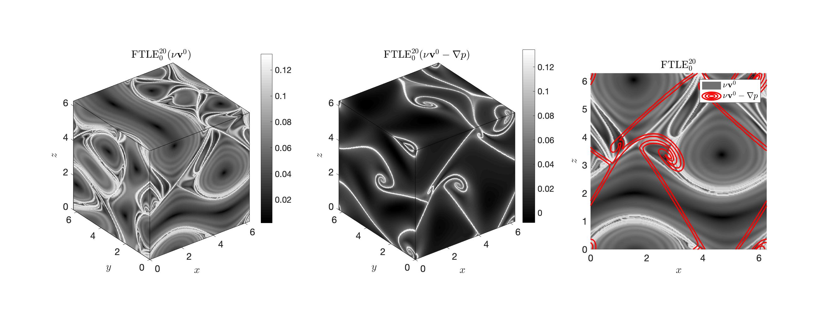
Figure 18: Comparison of structurally stable transport barriers as identified by FTLE. L to R: Barriers to diffusive momentum flux. Barriers to total momentum flux after including the pressure gradient. Comparison of diffusive and total momentum barriers on the $y=2\pi$ plane.

We note that for the turbulent channel flow of focus here, the streamwise velocity gradient is predominantly orthogonal to the pressure gradient. Thus, the shear-interfaces used to delineate uniform momentum zones actually maximize the total momentum transport through them.

Following these discussions and the connections drawn between momentum zones and experimentally observable barriers (Westerweel et al., 2009), we find that our definition of active transport that focuses on surfaces that block the viscous transport (as opposed to the total transport) of momentum and vorticity is the correct one for the purposes of structure identification that is experimentally reproducible.

References

- Adrian (2007) Adrian, Ronald J. 2007 Hairpin vortex organization in wall turbulence. Physics of Fluids 19 (4), 041301.
- Adrian et al. (2000a) Adrian, R. J., Christensen, K. T. & Liu, Z. C. 2000a Analysis and interpretation of instantaneous turbulent velocity fields. Experiments in Fluids 29 (3), 275–290.
- Adrian et al. (2000b) Adrian, R. J., Meinhart, C. D. & Tomkins, C. D. 2000b Vortex organization in the outer region of the turbulent boundary layer. Journal of Fluid Mechanics 422, 1–54.
- Astarita (1979) Astarita, Gianni 1979 Objective and generally applicable criteria for flow classification. Journal of Non-Newtonian Fluid Mechanics 6 (1), 69–76.
- Bandyopadhyay (1980) Bandyopadhyay, Promode 1980 Large structure with a characteristic upstream interface in turbulent boundary layers. Physics of Fluids 23 (11), 2326–2327.
- Bautista et al. (2019) Bautista, J. C. C., Ebadi, A., White, C. M., Chini, G. P. & Klewicki, J. C 2019 A uniform momentum zone-vortical fissure model of the turbulent boundary layer. Journal of Fluid Mechanics 858, 609–633.
- Beron-Vera et al. (2018) Beron-Vera, F. J., Hadjighasem, A., Xia, Q., Olascoaga, M. J. & Haller, G. 2018 Coherent Lagrangian swirls among submesoscale motions. Proceedings of the National Academy of Sciences 116 (37), 201701392.
- Chauhan et al. (2014) Chauhan, Kapil, Philip, Jimmy, De Silva, Charitha M., Hutchins, Nicholas & Marusic, Ivan 2014 The turbulent/non-turbulent interface and entrainment in a boundary layer. Journal of Fluid Mechanics 742, 119–151.
- Da Silva et al. (2014) Da Silva, C. B., Hunt, J. C.R., Eames, I. & Westerweel, J. 2014 Interfacial Layers Between Regions of Different Turbulence Intensity. Annual Review of Fluid Mechanics 46 (1), 567–590.
- De Silva et al. (2015) De Silva, C. M., Hutchins, N. & Marusic, I. 2015 Uniform momentum zones in turbulent boundary layers. Journal of Fluid Mechanics 786, 309–331.
- De Silva et al. (2017) De Silva, Charitha M., Philip, Jimmy, Hutchins, Nicholas & Marusic, Ivan 2017 Interfaces of uniform momentum zones in turbulent boundary layers. Journal of Fluid Mechanics 820, 451–478.
- Dennis & Nickels (2011) Dennis, David J.C. & Nickels, Timothy B. 2011 Experimental measurement of large-scale three-dimensional structures in a turbulent boundary layer. Part 1. Vortex packets. Journal of Fluid Mechanics 673, 180–217.
- Dong & Tian (2020) Dong, Yinlin & Tian, Wufeng 2020 On the thresholds of vortex visualisation methods. International Journal of Computational Fluid Dynamics 34 (4), 267–277.
- Drouot (1976) Drouot, R. 1976 Definition d’un transport associe un modele de fluide de deuxieme ordre. C. R. Acad. Sci. Pari Ser. A 282, 923–926.
- Drouot & Lucius (1976) Drouot, R. & Lucius, M. 1976 Approximation du second ordre de la loi de comportement des fluides simples. Lois classiques deduites de l’introduction d’un nouveau tenseur objectif. Arch. Mech. Stos. 28 (2), 189=198.
- Dubief & Delcayre (2000) Dubief, Y. & Delcayre, F. 2000 On coherent-vortex identification in turbulence. Journal of Turbulence 1 (2000).
- Eisma et al. (2015) Eisma, Jerke, Westerweel, Jerry, Ooms, Gijs & Elsinga, Gerrit E 2015 Interfaces and internal layers in a turbulent boundary layer. Physics of Fluids 27.
- Eisma et al. (2021) Eisma, Jerke, Westerweel, Jerry & van de Water, Willem 2021 Do coherent structures organize scalar mixing in a turbulent boundary layer? Journal of Fluid Mechanics 929, 1–19.
- Eyink et al. (2020) Eyink, Gregory L., Gupta, Akshat & Zaki, Tamer A. 2020 Stochastic Lagrangian dynamics of vorticity. Part 2. Application to near-wall channel-flow turbulence. Journal of Fluid Mechanics 901.
- Falco (1974) Falco, R. 1974 Some comments on turbulent boundary layer structure inferred from the movements of a passive contaminant. In AIAA 12th Aerospace Science Meeting, pp. 1–5. Washington D.C.
- Falco (1977) Falco, R. E. 1977 Coherent motions in the outer region of turbulent boundary layers. Physics of Fluids 20 (10).
- Fan et al. (2019) Fan, Duosi, Xu, Jinglei, Yao, Matthew X. & Hickey, Jean Pierre 2019 On the detection of internal interfacial layers in turbulent flows. Journal of Fluid Mechanics pp. 198–217, arXiv: 1811.09258.
- Farazmand & Haller (2016) Farazmand, Mohammad & Haller, George 2016 Polar rotation angle identifies elliptic islands in unsteady dynamical systems. Physica D: Nonlinear Phenomena 315, 1–12, arXiv: 1503.05970.
- Fiedler & Head (1966) Fiedler, H. & Head, M. R. 1966 Intermittency measurements in the turbulent boundary layer. Journal of Fluid Mechanics 25 (4), 719–735.
- Ganapathisubramani et al. (2006) Ganapathisubramani, Bharathram, Longmire, Ellen K. & Marusic, Ivan 2006 Experimental investigation of vortex properties in a turbulent boundary layer. Physics of Fluids 18 (5).
- Gao et al. (2011) Gao, Q., Ortiz-Dueñs, C. & Longmire, E. K. 2011 Analysis of vortex populations in turbulent wall-bounded flows. Journal of Fluid Mechanics 678, 87–123.
- Graham et al. (2016) Graham, J., Kanov, K., Yang, X.I.A., Lee, M.K., Malaya, N., Lalescu, C.C., Burns, R., Eyink, G., Szalay, A., Moser., R.D. & Meneveau, C. 2016 A Web Services-accessible database of turbulent channel flow and its use for testing a new integral wall model for LES. Journal of Turbulence 17 (2), 181–215.
- Green et al. (2007) Green, M. A., Rowley, C. W. & Haller, G. 2007 Detection of Lagrangian coherent structures in three-dimensional turbulence. Journal of Fluid Mechanics 572, 111–120, arXiv: arXiv:1104.5519v2.
- Gul et al. (2020) Gul, M., Elsinga, G.E. & Westerweel, J. 2020 Internal Shear Layers and Edges of Unifrom Momentum Zones in a Turbulent Pipe Flow. Journal of Fluid Mechanics 901 (A10).
- Günther & Theisel (2018) Günther, Tobias & Theisel, Holger 2018 The State of the Art in Vortex Extraction. Computer Graphics Forum 37 (6), 149–173.
- Haller (2005) Haller, G. 2005 An objective definition of a vortex. Journal of Fluid Mechanics 525, 1–26.
- Haller (2015) Haller, G. 2015 Lagrangian Coherent Structures. Annual review of fluid mechanics pp. 137–162.
- Haller (2021) Haller, George 2021 Can vortex criteria be objectivized? Journal of Fluid Mechanics 908 (A25).
- Haller et al. (2021) Haller, George, Aksamit, Nikolas & Bartos, Alex P. Encinas 2021 Quasi-Objective Coherent Structure Diagnostics from Single Trajectories. Chaos 31, 043131–1–17, arXiv: 2101.05903.
- Haller et al. (2016) Haller, G., Hadjighasem, A., Farazmand, M. & Huhn, F. 2016 Defining coherent vortices objectively from the vorticity. Journal of Fluid Mechanics 795, 136–173, arXiv: 1506.04061.
- Haller et al. (2018) Haller, George, Karrasch, Daniel & Kogelbauer, Florian 2018 Material barriers to diffusive and stochastic transport. Proceedings of the National Academy of Sciences 115 (37), 9074–9079, arXiv: 1803.11502.
- Haller et al. (2020) Haller, G., Katsanoulis, S., Holzner, M., Frohnapfel, B. & Gatti, D. 2020 Objective material barriers to the transport of momentum and vorticity. Journal of Fluid Mechanics .
- He et al. (2016) He, Guo Sheng, Pan, Chong, Feng, Li Hao, Gao, Qi & Wang, Jin Jun 2016 Evolution of Lagrangian coherent structures in a cylinder-wake disturbed flat plate boundary layer. Journal of Fluid Mechanics 792, 274–306.
- Head & Bandyopadhyay (1981) Head, M. R. & Bandyopadhyay, P. 1981 New aspects of turbulent boundary-layer structure. Journal of Fluid Mechanics 107 (11), 297–338.
- Holzner et al. (2006) Holzner, M., Liberzon, A., Guala, M., Tsinober, A. & Kinzelbach, W. 2006 Generalized detection of a turbulent front generated by an oscillating grid. Experiments in Fluids 41 (5), 711–719.
- Hommema & Adrian (2003) Hommema, Scott E. & Adrian, Ronald J. 2003 Packet structure of surface eddies in the atmospheric boundary layer. Boundary-Layer Meteorology 106 (1), 147–170.
- Hunt & Durbin (1999) Hunt, J. C.R. & Durbin, P. A. 1999 Perturbed vortical layers and shear sheltering. Fluid Dynamics Research 24 (6), 375–404.
- Hunt et al. (1988) Hunt, J. C. R., Wray, A. A. & Moin, P 1988 Eddies, streams, and convergence zones in turbulent flows. Center for Turbulence Research, Proceedings of the Summer Program pp. 193–208.
- Hwang & Sung (2018) Hwang, Jinyul & Sung, Hyung Jin 2018 Wall-attached structures of velocity fluctuations in a turbulent boundary layer. Journal of Fluid Mechanics 856, 958–983.
- Jeong & Hussain (1995) Jeong, J. & Hussain, F. 1995 On the Identification of a vortex. Jounral of Fluid Mechanics 285, 69–94.
- Jie et al. (2021) Jie, Yucheng, Andersson, Helge I. & Zhao, Lihao 2021 Effects of the quiescent core in turbulent channel flow on transport and clustering of inertial particles. International Journal of Multiphase Flow 140, 103627.
- Kirwan (2016) Kirwan, A. D. 2016 On objectivity, irreversibility and non-Newtonian fluids. Fluids 1 (1), 1–14.
- Kline et al. (1967) Kline, S. J., Reynolds, W. C., Schraub, F. A. & Runstadler, P. W. 1967 The structure of turbulent boundary layers. Journal of Fluid Mechanics 30 (4), 741–773.
- Kwon et al. (2016) Kwon, Y. S., Hutchins, N. & Monty, J. P. 2016 On the use of the Reynolds decomposition in the intermittent region of turbulent boundary layers. Journal of Fluid Mechanics 794, 5–16.
- Kwon et al. (2014) Kwon, Y. S., Philip, J., De Silva, C. M., Hutchins, N & Monty, J P 2014 The quiescent core of turbulent channel flow. Journal of Fluid Mechanics 751, 228–254.
- Laskari et al. (2018) Laskari, A., De Kat, R., Hearst, R. J. & Ganapathisubramani, B. 2018 Time evolution of uniform momentum zones in a turbulent boundary layer. Journal of Fluid Mechanics 842, 554–590.
- Li et al. (2008) Li, Y., Perlman, E., Wan, M., Yang, Y., Burns, R., Meneveau, C., Burns, R., Chen, S., Szalay, A. & Eyink, G. 2008 A public turbulence database cluster and applications to study Lagrangian evolution of velocity increments in turbulence. Journal of Turbulence 9 (31).
- Liu et al. (2019a) Liu, Jianming, Gao, Yisheng & Liu, Chaoqun 2019a An objective version of the Rortex vector for vortex identification. Physics of Fluids 31 (6).
- Liu et al. (2019b) Liu, Jianming, sheng Gao, Yi, qian Wang, Yi & Liu, Chaoqun 2019b Objective Omega vortex identification method. Journal of Hydrodynamics 31 (3), 455–463.
- Lugt (1979) Lugt, H.J. 1979 The Dilemma of Defining a Vortex. In Recent Developments in Theoretical and Experimental Fluid Mechanics (ed. Schmidt B. Müller U., Roesner K.G.). Berlin, Heidelberg: Springer.
- Marusic (2001) Marusic, I. 2001 On the role of large-scale structures in wall turbulence. Physics of Fluids 13 (3), 735–743.
- Marusic & Monty (2019) Marusic, Ivan & Monty, Jason P. 2019 Attached Eddy Model of Wall Turbulence. Annual Review of Fluid Mechanics 51 (1), 49–74.
- Meinhart & Adrian (1995) Meinhart, Carl D. & Adrian, Ronald J. 1995 On the existence of uniform momentum zones in a turbulent boundary layer. Physics of Fluids 7 (4), 694–696.
- Montemuro et al. (2020) Montemuro, Brandon, White, Christopher M., Klewicki, Joseph C. & Chini, Gregory P. 2020 A self-sustaining process theory for uniform momentum zones and internal shear layers in high Reynolds number shear flows. Journal of Fluid Mechanics 901, arXiv: 2006.15801.
- Neamtu-Halic et al. (2019) Neamtu-Halic, M. M., Krug, D., Haller, G. & Holzner, M. 2019 Lagrangian coherent structures and entrainment near the turbulent/non-Turbulent interface of a gravity current. Journal of Fluid Mechanics 877, 824–843.
- Offen & Kline (1974) Offen, G. R. & Kline, S. J. 1974 Combined dye-streak and hydrogen-bubble visual observations of a turbulent boundary layer. Journal of Fluid Mechanics 62 (2), 223–239.
- Pan et al. (2009) Pan, Chong, Wang, Jin Jun & Zhang, Cao 2009 Identification of lagrangian coherent structures in the turbulent boundary layer. Science in China, Series G: Physics, Mechanics and Astronomy 52 (2), 248–257.
- Peacock et al. (2015) Peacock, T., Froyland, G. & Haller, G. 2015 Introduction to focus issue: Objective detection of coherent structures. Chaos 25 (8).
- Perlman et al. (2007) Perlman, E., Burns, R., Li, Y. & Meneveau, C. 2007 Data Exploration of Turbulence Simulations using a Database Cluster. Supercomputing SC07, ACM, IEEE .
- Perry & Chong (1982) Perry, A. E. & Chong, M. S. 1982 On the mechanism of wall turbulence. Journal of Fluid Mechanics 119, 173–217.
- Raffel et al. (2018) Raffel, Markus, Willert, Christian E., Scarano, Fulvio, Kähler, Christian J., Wereley, Steven T. & Kompenhans, Jürgen 2018 Techniques for 3D-PIV. In Particle Image Velocimetry, pp. 309–365. Springer.
- Saxton-Fox & McKeon (2017) Saxton-Fox, Theresa & McKeon, Beverley J. 2017 Coherent structures, uniform momentum zones and the streamwise energy spectrum in wall-bounded turbulent flows. Journal of Fluid Mechanics 826, 1–12.
- Serra et al. (2017) Serra, M., Sathe, P., Beron-Vera, F. & Haller, G. 2017 Uncovering the edge of the polar vortex. Journal of the Atmospheric Sciences 74 (11), 3871–3885.
- Serra et al. (2020) Serra, M., Sathe, P., Rypina, I., Kirincich, A., Ross, S. D., Lermusiaux, P., Allen, A., Peacock, T. & Haller, G. 2020 Search and rescue at sea aided by hidden flow structures. Nature Communications 11 (1).
- Townsend (1976) Townsend, A.A. 1976 The Structure of Turbulent Shear Flow, second edi edn. New York, NY: Cambridge University Press.
- Westerweel et al. (2009) Westerweel, J., Fukushima, C., Pedersen, J. M. & Hunt, J. C.R. 2009 Momentum and scalar transport at the turbulent/non-turbulent interface of a jet. Journal of Fluid Mechanics 631, 199–230.
- Wilson et al. (2013) Wilson, Z. D., Tutkun, M. & Cal, R. B. 2013 Identification of Lagrangian coherent structures in a turbulent boundary layer. Journal of Fluid Mechanics 728, 396–416.
- Zhou et al. (1999) Zhou, J., Adrian, R. J., Balachandar, S. & Kendall, T. M. 1999 Mechanisms for generating coherent packets of hairpin vortices in channel flow. Journal of Fluid Mechanics 387, 353–396.