Low-rank projections of GCNs Laplacian

Abstract

In this work, we study the behavior of standard models for community detection under spectral manipulations. Through various ablation experiments, we evaluate the impact of bandpass filtering on the performance of a GCN: we empirically show that most of the necessary and used information for nodes classification is contained in the low-frequency domain, and thus contrary to images, high frequencies are less crucial to community detection. In particular, it is sometimes possible to obtain accuracies at a state-of-the-art level with simple classifiers that rely only on a few low frequencies.

1 Introduction

Graph Convolutional Networks (GCNs) are the state of the art in community detection (Kipf & Welling, 2016). They correspond to Graph Neural Networks (GNNs) that propagate graph features through a cascade of linear operator and non-linearities, while exploiting the graph structure through a linear smoothing operator. However, the principles that allow GCNs to obtain good performances remain unclear. Our work actually suggests that, in the setting of community detection, graph Laplacian high frequencies have actually a minor impact on the classification performances of a standard GCN, as opposed to standard Convolutional Neural Networks for vision.

Spectral clustering is a rather different point of view from deep supervised GCNs which studies node labeling in unsupervised contexts: it generally relies on generative models based on the graph spectrum. Our paper proposes to establish a clear link between these approaches: we show that the informative graph features are located in a low-frequency band of the graph Laplacian and can be efficiently used in a deep supervised classifier.

This paper shows that experiments on standard community detection datasets like Cora, Citeseer, Pubmed can be conducted using only few frequencies of their respective graph spectrum without observing any significant performances drop. Other contributions are as follows: (a) First we show that most of the necessary information exploited by a GCN for a community detection task can actually be isolated in the very first eigenvectors of a Laplacian. (b) We observe that a simple Multi-Layer Perceptron (MLP) method fed with handcrafted features accounting for low-frequency eigenvalues allows to successfully deal with transdusctive datasets like Cora, Citeseer or Pubmed.

2 Related Work

GCNs and Spectral GCNs

Introduced in Kipf & Welling (2016), GCNs allow to deal with large graph structure in semi-supervised classification contexts. This type of model works at the node level, meaning that it uses locally the adjacency matrix. This approach has inspired a wide range of models, such as linear GCN (Wu et al., 2019), Graph Attention Networks (Veličković et al., 2017), GraphSAGE (Hamilton et al., 2017), etc. In general, this line of work does not consider directly the graph Laplacian. Another line of work corresponds to spectral methods, taking inspiration from Graph Signal Processing (GSP), a popular field whose objective is to manipulate signals spectrum whose topology is given by a graph. They employ filters which are designed from the spectrum of a graph Laplacian (Bruna et al., 2013; Oyallon, 2020; 2017; Grinsztajn et al., 2021). In general, those works make use of polynomials in the Laplacian  (Defferrard et al., 2016) . All those references share the idea to manipulate bandpass filters that discriminate the different ranges of frequencies.

Over-smoothing in GCNs

In the context of GCN, Li et al. (2018) is one of the first papers to notice that cascading low-pass filters can lead to a substantial information loss. The result of our work indicates that the important spectral components for detecting communities are already in the low-frequency domain and that this is not due to an architecture bias. Zhao & Akoglu (2019); Yang et al. (2020) propose to introduce regularizations which address the loss of information issues. Cai & Wang (2020); Oono & Suzuki (2019) study the spectrum of a graph Laplacian under various transforms, yet they consider the spectrum globally and in asymptotic settings, with a deep cascade of layers. Huang et al. (2020); Rong et al. (2019) introduce data augmentations, whose aim is to alleviate over-smoothing in deep networks: we study GCNs without this ad-hoc procedure.

Spectral clustering and low rank approximation

As the literature about spectral clustering is large, we mainly focus on the subset that connects directly with GCN. Mehta et al. (2019) proposes to learn an unsupervised auto-encoder in the framework of a Stochastic Block Model. Oono & Suzuki (2019) introduces the Erdös – Renyi model in the GCN analysis, but only in an asymptotic setting. Loukas & Vandergheynst (2018) studies the graph topology preservation under the coarsening of the graph, which could be a potential direction for future works. Liao et al. (2019) uses the Lanczos algorithm to construct low rank approximations of the graph Laplacian, which facilitates efficient computation of matrix powers.

Node embedding

A MLP approach can be understood as an embedding at the node level. For instance, Aubry et al. (2011) applies a spectral embedding combined with a diffusion process for shape analysis, which allows point-wise comparisons. We also mention Deutsch & Soatto (2020) that uses a node embedding, based on the spectrum of a quite modified graph Laplacian, obtained from on a measure of node centrality.

GCN stability

Stability of GCNs has been theoretically studied in Gama et al. (2019), which shows that defining a generic notion of deformations is difficult. Surprisingly, it was noted in Oyallon (2020) that stability is not a key component to good performances. The stability of GCN has also been investigated in Verma & Zhang (2019) but only considers neural networks with a single layer and relies on the whole spectrum of the learned layer. Keriven et al. (2020) considers the stability of GCNs, and relies on an implicit Euclidean structure: it is unclear if this holds in our settings. Sun et al. (2020) is one of the first works to study adversarial examples linked to the node connectivity and introduces a loss to reduce their effects. Zhu et al. (2019) also addresses the stability issues by embedding GCNs in a continuous representation. None of these work directly related a trained GCN to spectral perturbations.

3 Framework

3.1 Method

We first describe our baseline model. Our initial graph data are a graph with $N$ nodes, its adjacency matrix $A$ with diagonal degree matrix $D$, and node features $X$. We consider first-order GCNs as introduced in (Kipf & Welling, 2016), which correspond to GNNs that propagate node feature input $H^{(0)}\triangleq X$ through a cascade of layers, via the iteration:

$$H^{(l+1)}\triangleq\sigma\bigg{(}\tilde{A}H^{(l)}W^{(l)}\bigg{)}\,,$$ (1)

where $\tilde{A}=\frac{1}{2}(I+D^{-1/2}AD^{-1/2})$, $\sigma$ a point-wise non-linearity and $W^{(l)}$ a parametrized affine operator. Note that if $\tilde{A}=I_{N}$, then Eq. 1 is simply an MLP. The $\frac{1}{2}$ factor is a normalization factor to obtain $\|\tilde{A}\|=1$. In the semi-supervised setting, a final layer $f(X,\tilde{A})\triangleq H^{(L)}$ is fed to a supervised loss $\ell$ (here a softmax) and $\{W^{(0)},...,W^{L-1}\}$ are trained in an end-to-end manner to adjust the label of each node. We note that for undirected graph, $\tilde{A}$ is a positive definite matrix with positive weights, which can be understood as an averaging operator (Li et al., 2018).

We are interested in analyzing the properties of spectral approximations of $\tilde{A}$. We consider the decreasing set of eigenvalues $\Lambda=\{\lambda_{k}\}_{k\geq 0}$ of $\tilde{A}$, such that $\lambda_{k}\geq\lambda_{k+1}$, and we denote by $u_{k}$ the $k$-th eigenvector corresponding to $\lambda_{k}\in\Lambda$. We remind that $\Lambda\subset[0,1]$ and that the eigenspace corresponding to $\lambda=1$ can be interpreted as the kernel of the symmetric normalized graph Laplacian. We then write $\tilde{A}_{[k_{1},k_{2}]}\triangleq\sum_{k_{1}\leq k\leq k_{2}}\lambda_{k}u_{k}u_{k}^{T}$ , such that $\tilde{A}=\tilde{A}_{[0,N]}$. We are interested in studying the degradation accuracy if we replace $\tilde{A}$ with $\tilde{A}_{[0,k]}$ or $\tilde{A}_{[k,N]}$ for some $0<k<N$.

4 Experiments

Matching the previous work practice, we focus on the three classical benchmark dataset for community detection: Cora, Citeseer and Pubmed (Sen et al., 2008). The task consists in classifying the research topic of papers in three citation datasets. Those tasks are transductive, meaning all node features are accessible during training. We use the same training/validation/test split as Huang et al. (2018a), Chen et al. (2018), and Rong et al. (2019) on all datasets in our experiments, which corresponds to a supervised learning scenario. The statistics of each dataset are listed in the supplemental materials, as well as the training details.

4.1 Low rank approximation

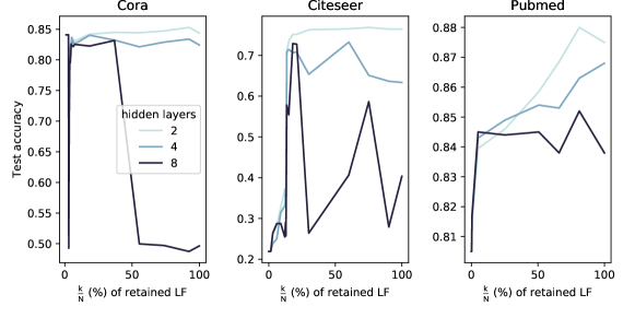
Figure 1: Test accuracies reached by a GCN as a function of the Low-Frequency (LF) band $[\lambda_{k},\lambda_{0}]$ retained by $\tilde{A}_{[0,k]}$, for various depths (100$\%$ corresponds to the full spectrum, including low frequencies). This figure indicates that the informative components are located in the LF domain.

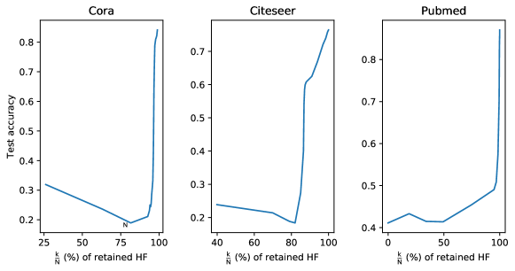
Figure 2: Test accuracies reached by a GCN as a function of the high frequencies (HF) band $[\lambda_{N},\lambda_{N-k}]$ retained by $\tilde{A}_{[N-k,N]}$, for a GCN of depth 2 (100$\%$ corresponds to the full spectrum). This figure indicates that high frequencies are less informative for a community detection task.

GCN ablation

Here, we consider the two projections $\tilde{A}_{[0,k]}$ and $\tilde{A}_{[N-k,N]}$, where $k$ is adjusted to retain only a portion of the spectrum. Those projections can be interpreted respectively as high-pass and low-pass filters. As detailed in Appendix C, those projections will allow to study which frequency band is important for the community detection task. Fig. 1 and Fig. 2 report the respective performance when considering the models $f(X,\tilde{A}_{[N-k,N]})$ and $f(X,\tilde{A}_{[0,k]})$ for some $k$. On Fig. 1, we observe that retaining only very few frequencies (less than 10%) does not degrade much the accuracy of the original network. This does not contradict the observation of Li et al. (2018) which studies empirically the over-smoothing phenomenon, as our finding indicates that a GCN uses mainly the low frequency domain. For Pubmed, using almost all the high frequencies is required to recover the original accuracy of our model. Interestingly, deeper GCNs seem to benefit from the high frequency ablation, yet their accuracy remains below their shallow counter-part and they are still difficult to train. This instability to spectral perturbations is further studied in Appendix D. Fig. 2 indicates that the major information for supervised community detection is contained in the low frequencies: dropping the latter leads to substantial accuracy drop, even for a shallow GCN.

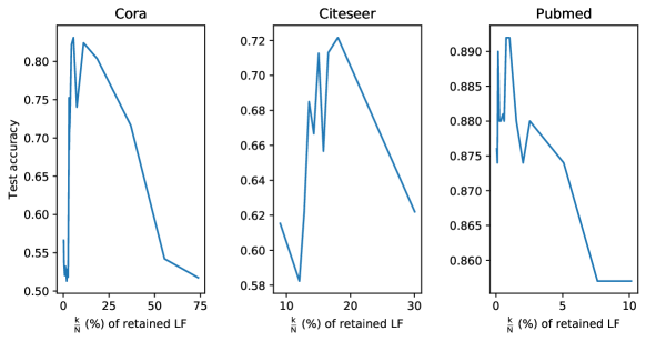
Figure 3: Accuracy of MLPs trained on $X_{k}$, according to the low frequency band $[\lambda_{k},\lambda_{0}]$ retained. We note that selecting a narrow low-frequency band can lead to competitive accuracies.

MLP augmentation

We further study the importance of low frequencies via a spare ablation experiment based on a MLP. We augment each graph features $X$ through the concatenation $X_{k}=[X,u_{1}^{T},...,u_{k}^{T}]$ of the first $k$ eigenvectors. Fig. 3 reports the accuracy of our MLP trained on $X_{k}$ as a function of $k$. We see that using a fraction $\frac{k}{N}\leq 20\%$ of the eigenvectors allows to recover the performance of a GCN. More surprisingly, we note that as $k$ increases, the accuracy drops, which indicates that high frequencies behave like a residual noise that is overfitted. This experiment emphasizes that a low rank approximation of the Laplacian can be beneficial to a MLP classifier.

Table 1: Comparison of various models on Cora, Citeseer and Pubmed.

Method	Data augmentation	Cora	Citeseer	Pubmed
GCN (Rong et al., 2019)	No	86.6	79.3	90.2
Fastgcn (Chen et al., 2018)	No	86.5	-	88.8
MLP on $X$	No	74.0	73.3	89.1
MLP on $\tilde{X}_{k}$ (ours)	No	86.6	77.3	91.4
DropEdge (Rong et al., 2019)	Yes	88.2	80.5	91.7
(Huang et al., 2018b)	Yes	87.4	79.7	90.6

Boosting MLP performances

We perform a hyper-parameter grid search on each dataset to investigate MLP strengths further. We summarize our findings in Tab. 1. In particular, one uses a fraction 6%, 15.0% and 0.7% of the spectrum respectively on Cora, Citeseer and Pubmed in order to obtain our best performances. More details on the methodology are provided in the supplementary material. This simple model is often competitive with concurrent works, and in particular with vanilla GCNs. Note also that our method does not incorporate any data augmentation procedure. We conclude that GCNs do not compute more complex invariants than a MLP fed with low frequencies, in the context of community detection.

5 Conclusion

We have studied the classification performance of a GCN under low-pass and high-pass filtering, in the context of community detection. Our finding is that GCNs rely significantly on the low frequencies, and can even benefit from high-frequency ablations. Then, we are able to design MLPs that rely simply on a few eigenvectors of the graph Laplacian and can be competitive with GCNs.

We observed that the high-frequency does not bring a significant amount of information, and can even be interpreted as a residual noise in this particular setting. Our methodology can also help to identify if the accuracy improvement of a new architecture is due to a better processing of high frequencies.

Acknowledgements

EO was granted access to the HPC resources of IDRIS under the allocation 2020-[AD011011216R1] made by GENCI and this work was partially supported by ANR-19-CHIA ”SCAI”. Experiments presented in this paper were partially carried out using the Grid’5000 testbed, supported by a scientific interest group hosted by Inria and including CNRS, RENATER and several Universities as well as other organizations. NG is recipient of a PhD funding from AMX program, Ecole polytechnique.

Appendix A Appendix

A.1 Dataset statistics

Table 2: Dataset Statistics

Datasets	Nodes	Edges	Classes	Features	Traing/Validation/Testing split
Cora	2,708	5,429	7	1,433	1,208/500/1,000
Citeseer	3,327	4,732	6	3,703	1,812/500/1,000
Pubmed	19,717	44,338	3	500	18,217/500/1,000

A.2 Spectra of Cora, Citeseer, Pubmed

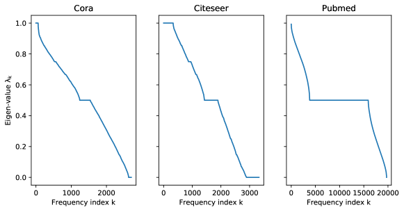
Figure 4: Spectrum $\Lambda$ of $\tilde{A}$. Note that the eigenvalues are decreasing, displayed with multiplicity. Observe that the decay of the spectrum is fast.

Appendix B Training Details

We choose $\sigma$ to be the ReLU non-linearity (Krizhevsky et al., 2012). Unless specified otherwise, the weights of our models (either GCN or MLP) are optimized via Adam, with an initial learning rate 0.01 and weight decay of 0.001, during 800 epochs. We use by default a dropout of 0.5. Our model consists in GCN layers with 2 hidden layers of size 128. When using grid search, we cross validate our hyper-parameters on a validation set, using early stopping with a patience of 400. The grid search is detailed in the following table. Unless specified otherwise, each plot is obtained by an average over 3 different seeds.

B.1 Hyper-parameter Description

Table 3: Hyper-parameter Description and Grid Search Range

Hyper-parameter	Description	Range
lr	learning rate	$\{0.01,0.001\}$
hidden layers	the number of hidden layers	$\{1,2,3,4\}$
weight-decay	L2 regulation weight	0.001
dropout	dropout rate	$\{0,0.2,0.4,0.6,0.8\}$
frequencies	the number of low frequencies to add (%)	$\{0.1,0.2,0.4,0.7,1,2,3,$
		$6,10,15,20,30,50,80,100\}$
eigenvector features normalization	whether to normalize the new MLP features	{ False, True }
	in line (per nodes) or column (per features)

Appendix C Understanding low rank approximations for GCNs

We now justify our approach under the standard setting of the Stochastic Block Model (Abbe, 2017), and we will simply remind the reader of several elementary results. This model corresponds to a generative model that describes the interaction between $r$ communities $\{C_{1},...,C_{r}\}$. Assuming that two nodes $i,j$ belong to the communities $C_{r_{i}},C_{r_{j}}$, an edge is sampled with a probability $p_{r_{i},r_{j}}$ (Rohe et al., 2011). For the sake of simplicity, let us assume that $r=2$, that the probability of an edge between two nodes $i,j$ is $p$ if those nodes belong to the same community and $q<p$ otherwise, and that both communities correspond to $|C|$ nodes. In this case, the unnormalized expected adjacency matrix is given by:

$$\begin{bmatrix}p&\cdots&p&q&\cdots&q\\ \vdots&&\vdots&\vdots&&\vdots\\ p&\cdots&p&q&\cdots&q\\ q&\cdots&q&p&\cdots&p\\ \vdots&&\vdots&\vdots&&\vdots\\ q&\cdots&q&p&\cdots&p\\ \end{bmatrix}\,,$$ (2)

where we grouped in matrix block the nodes from the same community. We note that the two dominant eigenvectors are given by:

$$u_{1}=[\overbrace{1,...,1,}^{|C|\text{ times}}\underbrace{1,...,1}_{|C|\text{ times}}]\text{ and }u_{2}=[\overbrace{1,...,1,}^{|C|\text{ times}}\underbrace{-1,...,-1}_{|C|\text{ times}}]\,.$$ (3)

Observe that the second eigenvector $u_{2}$ captures all the information about the two communities, through the sign of its coefficients. Here, the spectral gap (the ratio between the two dominant eigenvalues) is given by $0\leq\frac{p-q}{p+q}<1$ and ideally this spectral gap should be as large as possible for identifying the two communities. If the number of nodes is large, concentration results (Wainwright, 2019) imply that the empirical adjacency matrix concentrates around its expectation, and that under this assumption, a low-rank approximation $\tilde{A}_{[0,2]}$ captures most of the available information about the two communities. We illustrate this idea on Fig. 5. While these assumptions might not hold in practice, it justifies why low-rank approximations of a Laplacian are relevant in the setting of community detection and it explains why high frequencies might not be as important as low frequencies for supervised community detection task. The next section validates empirically this approach in the context of GCNs and simpler architectures.

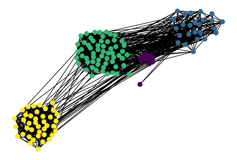
(a)

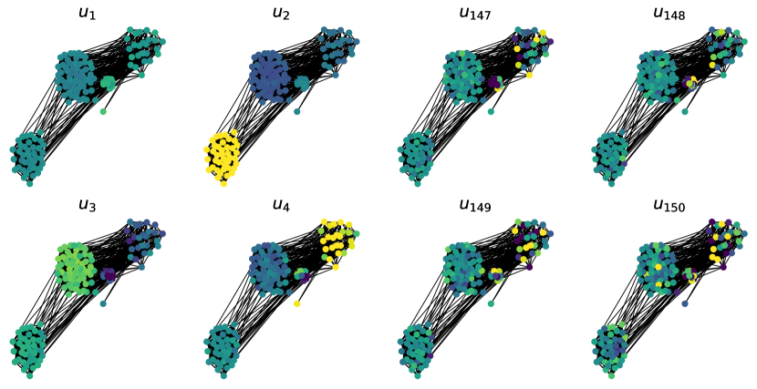
(b)

Figure 5: Under a Stochastic Block Model with 4 communities (a), we represent the first Eigenvectors (b, left) and the last Eigenvectors (b, right) of $\tilde{A}$. On the left figure, the colors stand for the communities. On the right, they stand for the values of the considered eigenvectors (the brighter the higher). A low rank approximation maintains the information related to the different communities.

Appendix D Stability to High Frequencies

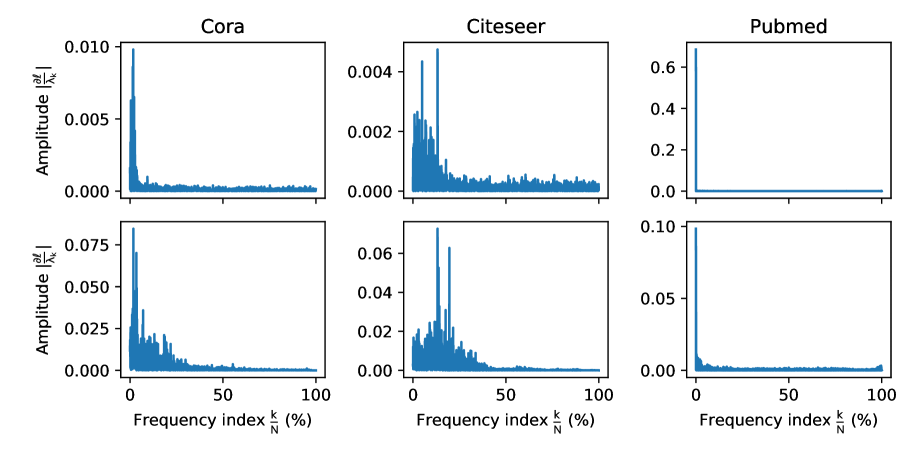
Figure 6: The (top) and (bottom) figures corresponds to $|\frac{\partial\ell}{\lambda_{k}}|$ of the same model taken respectively at the initialization and the end of training. Note that high frequencies are more stable than low frequencies for the three datasets.

We now study the stability of a GCN w.r.t. spectrum perturbations. In the case of image processing, it is standard that low frequencies almost do not affect the classification performances and that perturbations of high frequencies lead to instabilities. We would like to validate that this principle does not hold here, and to do so, we consider $\nabla_{\Lambda}\ell$, which is the gradient w.r.t. every singular value $\lambda_{k}$. Small amplitudes of $|\frac{\partial\ell}{\partial\lambda_{k}}|$ indicate more stable coefficients. Fig. 6 plots the amplitude of the gradient w.r.t. $\lambda_{k}$ at the initialization of a GCN and after training. First, we note that a GCN is more sensitive to spectral perturbations after training, which is logical because the GCN adapts its weights to the specific structure of a given graph. After training, we remark that the high-frequency perturbations have a small impact compared to the low-frequency perturbations on the three datasets, except for Pubmed which has dominant low frequencies. This is consistent with our previous findings.

Appendix E Note on the computational overhead

The MLPs introduced above are of interest if the corresponding graph topology is fixed, with a large graph, and high connectivity. Indeed, using a MLP allows to easily employ mini-batch strategies and the training data can be reduced according to the fraction of low frequencies being kept: an exact $k$-truncated SVD has a complexity about $\mathcal{O}(kN^{2})$. We note that fast $k$-truncated $\epsilon$-approximate SVD algrotithms for sparse matrix exist (Allen-Zhu & Li, 2016): if $\rho$ is the number of non-zero coefficients of $\tilde{A}$, the complexity can be about $\mathcal{O}(\frac{k\rho}{\epsilon}+\frac{k^{2}N}{\epsilon})$.

References

- Abbe (2017) Emmanuel Abbe. Community detection and stochastic block models: recent developments. The Journal of Machine Learning Research, 18(1):6446–6531, 2017.
- Allen-Zhu & Li (2016) Zeyuan Allen-Zhu and Yuanzhi Li. Lazysvd: Even faster svd decomposition yet without agonizing pain. In Advances in Neural Information Processing Systems, pp. 974–982, 2016.
- Aubry et al. (2011) Mathieu Aubry, Ulrich Schlickewei, and Daniel Cremers. The wave kernel signature: A quantum mechanical approach to shape analysis. In 2011 IEEE international conference on computer vision workshops (ICCV workshops), pp. 1626–1633. IEEE, 2011.
- Bruna et al. (2013) Joan Bruna, Wojciech Zaremba, Arthur Szlam, and Yann LeCun. Spectral networks and locally connected networks on graphs. arXiv preprint arXiv:1312.6203, 2013.
- Cai & Wang (2020) Chen Cai and Yusu Wang. A note on over-smoothing for graph neural networks. arXiv preprint arXiv:2006.13318, 2020.
- Chen et al. (2018) Jie Chen, Tengfei Ma, and Cao Xiao. Fastgcn: Fast learning with graph convolutional networks via importance sampling. CoRR, abs/1801.10247, 2018. URL http://arxiv.org/abs/1801.10247.
- Defferrard et al. (2016) Michaël Defferrard, Xavier Bresson, and Pierre Vandergheynst. Convolutional neural networks on graphs with fast localized spectral filtering. In Advances in neural information processing systems, pp. 3844–3852, 2016.
- Deutsch & Soatto (2020) Shay Deutsch and Stefano Soatto. Spectral embedding of graph networks, 2020.
- Gama et al. (2019) Fernando Gama, Joan Bruna, and Alejandro Ribeiro. Stability properties of graph neural networks. arXiv preprint arXiv:1905.04497, 2019.
- Grinsztajn et al. (2021) Nathan Grinsztajn, Louis Leconte, Philippe Preux, and Edouard Oyallon. Interferometric graph transform for community labeling. In arXiv preprint, 2021.
- Hamilton et al. (2017) Will Hamilton, Zhitao Ying, and Jure Leskovec. Inductive representation learning on large graphs. In Advances in neural information processing systems, pp. 1024–1034, 2017.
- Huang et al. (2018a) Wen-bing Huang, Tong Zhang, Yu Rong, and Junzhou Huang. Adaptive sampling towards fast graph representation learning. CoRR, abs/1809.05343, 2018a. URL http://arxiv.org/abs/1809.05343.
- Huang et al. (2018b) Wenbing Huang, Tong Zhang, Yu Rong, and Junzhou Huang. Adaptive sampling towards fast graph representation learning. In Advances in neural information processing systems, pp. 4558–4567, 2018b.
- Huang et al. (2020) Wenbing Huang, Yu Rong, Tingyang Xu, Fuchun Sun, and Junzhou Huang. Tackling over-smoothing for general graph convolutional networks, 2020.
- Keriven et al. (2020) Nicolas Keriven, Alberto Bietti, and Samuel Vaiter. Convergence and stability of graph convolutional networks on large random graphs, 2020.
- Kipf & Welling (2016) Thomas N Kipf and Max Welling. Semi-supervised classification with graph convolutional networks. arXiv preprint arXiv:1609.02907, 2016.
- Krizhevsky et al. (2012) Alex Krizhevsky, Ilya Sutskever, and Geoffrey E Hinton. Imagenet classification with deep convolutional neural networks. In Advances in neural information processing systems, pp. 1097–1105, 2012.
- Li et al. (2018) Qimai Li, Zhichao Han, and Xiao-Ming Wu. Deeper insights into graph convolutional networks for semi-supervised learning. arXiv preprint arXiv:1801.07606, 2018.
- Liao et al. (2019) Renjie Liao, Zhizhen Zhao, Raquel Urtasun, and Richard Zemel. Lanczosnet: Multi-scale deep graph convolutional networks. In International Conference on Learning Representations, 2019. URL https://openreview.net/forum?id=BkedznAqKQ.
- Loukas & Vandergheynst (2018) Andreas Loukas and Pierre Vandergheynst. Spectrally approximating large graphs with smaller graphs. arXiv preprint arXiv:1802.07510, 2018.
- Mehta et al. (2019) Nikhil Mehta, Lawrence Carin, and Piyush Rai. Stochastic blockmodels meet graph neural networks. arXiv preprint arXiv:1905.05738, 2019.
- Oono & Suzuki (2019) Kenta Oono and Taiji Suzuki. Graph neural networks exponentially lose expressive power for node classification. arXiv preprint arXiv:1905.10947, 2019.
- Oyallon (2017) Edouard Oyallon. Analyzing and introducing structures in deep convolutional neural networks. PhD thesis, Paris Sciences et Lettres, 2017.
- Oyallon (2020) Edouard Oyallon. Interferometric graph transform: a deep unsupervised graph representation. In Proceedings of Machine Learning and Systems 2020, pp. 4124–4134. 2020.
- Rohe et al. (2011) Karl Rohe, Sourav Chatterjee, Bin Yu, et al. Spectral clustering and the high-dimensional stochastic blockmodel. The Annals of Statistics, 39(4):1878–1915, 2011.
- Rong et al. (2019) Yu Rong, Wenbing Huang, Tingyang Xu, and Junzhou Huang. Dropedge: Towards deep graph convolutional networks on node classification. In International Conference on Learning Representations, 2019.
- Sen et al. (2008) Prithviraj Sen, Galileo Namata, Mustafa Bilgic, Lise Getoor, Brian Galligher, and Tina Eliassi-Rad. Collective classification in network data. AI Magazine, 29(3):93, Sep. 2008. doi: 10.1609/aimag.v29i3.2157. URL https://www.aaai.org/ojs/index.php/aimagazine/article/view/2157.
- Sun et al. (2020) Ke Sun, Piotr Koniusz, and Zhen Wang. Fisher-bures adversary graph convolutional networks. In Uncertainty in Artificial Intelligence, pp. 465–475. PMLR, 2020.
- Veličković et al. (2017) Petar Veličković, Guillem Cucurull, Arantxa Casanova, Adriana Romero, Pietro Lio, and Yoshua Bengio. Graph attention networks. arXiv preprint arXiv:1710.10903, 2017.
- Verma & Zhang (2019) Saurabh Verma and Zhi-Li Zhang. Stability and generalization of graph convolutional neural networks. In Proceedings of the 25th ACM SIGKDD International Conference on Knowledge Discovery & Data Mining, pp. 1539–1548, 2019.
- Wainwright (2019) Martin J Wainwright. High-dimensional statistics: A non-asymptotic viewpoint, volume 48. Cambridge University Press, 2019.
- Wu et al. (2019) Felix Wu, Amauri H Souza Jr, Tianyi Zhang, Christopher Fifty, Tao Yu, and Kilian Q Weinberger. Simplifying graph convolutional networks. In ICML, 2019.
- Yang et al. (2020) Chaoqi Yang, Ruijie Wang, Shuochao Yao, Shengzhong Liu, and Tarek Abdelzaher. Revisiting” over-smoothing” in deep gcns. arXiv preprint arXiv:2003.13663, 2020.
- Zhao & Akoglu (2019) Lingxiao Zhao and Leman Akoglu. Pairnorm: Tackling oversmoothing in gnns. arXiv preprint arXiv:1909.12223, 2019.
- Zhu et al. (2019) Dingyuan Zhu, Ziwei Zhang, Peng Cui, and Wenwu Zhu. Robust graph convolutional networks against adversarial attacks. In Proceedings of the 25th ACM SIGKDD International Conference on Knowledge Discovery & Data Mining, pp. 1399–1407, 2019.