qprof: a gprof-inspired quantum profiler

Abstract

We introduce qprof, a new and extensible quantum program profiler able to generate profiling reports of various quantum circuits. We describe the internal structure and working of qprof and provide three practical examples on practical quantum circuits with increasing complexity. This tool will allow researchers to visualise their quantum implementation in a different way and reliably localise the bottlenecks for efficient code optimisation.

I Introduction

The quantum computing field has been evolving at an increasing rate in the past few years and is currently gaining more traction. Several quantum chips, the underlying hardware that enable researchers and companies to run quantum algorithms, have been announced by different research teams. The error rates and number of qubits provided by these chips greatly improved, with quantum hardware that have up to $65$ qubits in early 2021.

Software has also seen a tremendous rise with the emergence of several quantum computing frameworks and languages such as Qiskit Abraham et al. (2019), Q# team (2021b), PyQuil Computing (2021), Cirq Cirq Developers (2021) or myQLM team (2021a) to name a few. These frameworks help in speeding-up the process of implementing a quantum algorithm by providing their own ”standard library”. Most of them also include specialised libraries whose purpose is to facilitate the development and testing of new quantum algorithms. For example, all the quantum computing frameworks cited previously include a library to simulate quantum circuits, some even implement several simulation algorithms such as a full state-vector simulator, a simulator for stabilizer circuits Aaronson and Gottesman (2004); Gidney (2021) or a simulator using matrix-product states as described in Vidal (2003); Schollwöck (2011). Most of the frameworks that target real quantum chips also include libraries to characterise a given quantum hardware, using for example randomised benchmarking Emerson et al. (2005); Knill et al. (2008); Gambetta et al. (2012); Cross et al. (2016); McKay et al. (2019) methods, or to mitigate hardware noise LaRose et al. (2020); Bravyi et al. (2021).

Finally, a large majority of the quantum computing frameworks provide a way to automatically optimise a quantum circuit. This optimisation is often performed during compilation, when the abstract quantum circuit representation is translated to be compliant with the targeted hardware. Automatic optimisation of quantum circuits is a broad area of research with algorithms based on pattern-matching Iten et al. (2019); Maslov et al. (2008); Nam et al. (2018), gate-based optimisation algorithms Fösel et al. (2021); Bae et al. (2020) or even pulse-based ones Shi et al. (2019); Gokhale et al. (2020); Earnest et al. (2021).

But even though automatic optimisation has already been shown to be successful in optimising complex quantum circuits Childs et al. (2018), most algorithms only perform local optimisations without any knowledge about the algorithms used and do not have a global vision of the optimised circuit. This means that automatic optimisation algorithms will likely not be able to perform some optimisations that require a global vision of the quantum circuit or a semantic understanding of the quantum algorithms used. Identifying the usage of a non-optimal algorithm in the implementation and replacing it with a more efficient algorithm is an example of such an optimisation that cannot be performed without a semantic understanding of the implementation.

Currently, the only other way one has to optimise a given quantum implementation is ”trial and error”: try to locate a ”hot spot” in the implementation, either by a tedious theoretical analysis or a manual counting of the routine calls, optimise the potential hot spot found and finally check if the optimisation performed improved the performances. This process has a severe drawback that makes it impractical on real-world implementations: the first step that consists in finding the hot spots is either imprecise or potentially very long, tedious and error-prone on large implementations.

qprof aims at replacing this manual, tedious and error-prone step of analysis by automatically generating a report with all the useful information needed to find the hot spots of the given quantum program implementation. The qprof tool has been strongly inspired by classical profilers such as gprof Graham et al. (1982); Foundation (2020a) which try to solve the exact same issue but in classical (non-quantum) programming.

The rest of the paper is organised as follows. In Section II we explain the internals of qprof and explain in details its architecture, the design choices made, and their impact on the tool efficiency, extensibility and usability. We then include code snippets and simple practical examples in Section III to illustrate the tool usage.

II How does qprof works?

II.1 General structure

The general structure of qprof is composed of 3 main parts that interact with each other: framework plugins, core data structures and logic, and exporters.

The overall workflow of qprof is schematically explained in Figure 1. In this workflow, qprof can be seen as a black-box that takes a ”quantum circuit” as input and returns a ”profiler report”. This black-box view should be enough for users that only want to use the qprof tool, but experienced users or plugins developers might need more details on the internals of qprof in order to understand how it works.

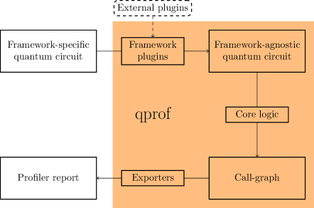
Figure 1: Schematic representation of qprof workflow. Highlighted portions are part of qprof.

The following sections will introduce in details the three different parts that compose qprof. Section II.2 describes the plugins architecture, used by qprof to be as modular and extensible as possible. Section II.3 then shows how this plugin architecture is used to allow qprof to be mostly framework-agnostic by allowing anyone to implement a framework without modifying qprof code. A description of the core data structures and core logic is then provided in Section II.4. Finally an explanation of the different exporters natively provided by qprof is given in Section II.5.

II.2 Plugin architecture

The qprof tool aims at being the standard for profiling quantum circuits, independently of the framework they are written with. In order to be versatile and support as much current and future quantum computing frameworks as possible, qprof has been designed to be easily extensible to support new frameworks.

qprof extensibility is achieved via a system of runtime-discovered plugins. In order to be discoverable by qprof, a plugin should naturally obey some rules such as implementing a specific interface (explained in Section II.3) or being organised in an imposed way. But the key ingredient to extensiblity is that plugins do not have to be part of the main qprof tool: they can be developed and published by anyone. This allows several situations that may help improving qprof stability and evolution in time. For example, users might decide to roll-out their own plugin to support a new framework they are using internally. Another important situation that is made possible by this plugin architecture is that framework vendors have the opportunity to provide a qprof plugin along with their framework and to maintain it as an official plugin.

Finally, such an architecture based on external plugins allows the user to only install the plugins and frameworks needed instead of installing all the plugins along with qprof. This simple side improvement greatly reduces the installation time, installation size and plugin discovery time as it avoids installing and loading unused quantum computing frameworks.

Observation 1.

Even though the reduction in installation time, size and loading time may seem negligible at first sight, we found out that avoiding some packages adds a significant improvement. For example, we computed that installing qiskit 0.24.1 with Python 3.8.8 on a modest laptop (MacBook Air from 2017) with a very good Internet connection takes more than 1 minute and ends up using more than 600 Mo of disk space. About run-time effects, importing the main qiskit package from a Python interpreter can take up to several seconds.

II.3 Framework support

The goal of the qprof tool is to provide a unique profiling interface for quantum programs. As such, it should be able to support as much quantum computing programming frameworks as possible. Taking into account that several of the most successful quantum computing frameworks such as Qiskit, Cirq, PyQuil or myQLM are Python libraries, and in order to ease its integration with these already existing frameworks, qprof has naturally been designed as a Python library too.

But being written in the same language as a given quantum computing framework does not grant a direct compatibility. In fact, all the previously cited frameworks use a different representation for quantum programs. Qiskit implements a QuantumCircuit class, Cirq comes with a Circuit class, PyQuil uses a Program structure and finally myQLM uses either QRoutine or AbstractGate instances.

To be as independent as possible from the different quantum computing frameworks and their internal representation of a quantum circuit, qprof has been designed to be both extensible and generic.

Extensibility is achieved with the help of the plugin architecture described in Section II.2. And in order to be as generic as possible, qprof uses an abstract common interface to represent the concept of ”quantum (sub)routine”. This concept is formally defined in Definitions 1, 2 and 3.

Definition 1.

Quantum routine: a (possibly parametrised) named sequence of quantum subroutines.

Definition 2.

Quantum subroutine: a quantum routine that is part of a higher-level quantum routine (i.e. that is called by another quantum routine).

Definition 3.

Native quantum subroutine: a quantum subroutine that represents a native hardware operation and that does not call any quantum subroutine.

Using Definitions 1, 2 and 3, a common interface for the concept of ”quantum routine” emerges. First, a quantum routine should have a name that can be retrieved. Secondly, we should be able to distinguish between native quantum subroutines and non-native ones. Finally, for non-native quantum subroutines, we need a way to iterate over all the subroutines composing it.

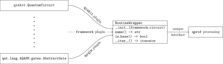
Figure 2: Schematic overview of the framework architecture used in qprof. Each framework-specific representation is wrapped by a RoutineWrapper. Each supported framework should have a corresponding qprof plugin that implements the RoutineWrapper interface. The __init__ method initialises a RoutineWrapper instance with an instance of the framework-specific quantum circuit representation. The name method returns the name of the currently wrapped routine. is_base returns True if the routine is a native subroutine as defined in Definition 3, else it returns False. Finally, the __iter__ method returns an object that can be iterated on and whose iterates are the different subroutines called by the current subroutine.

This interface, schematised in Figure 2, is the core abstraction layer of qprof that allows it to be as independent as possible from the underlying quantum computing framework used to represent the profiled quantum circuit.

II.4 Core data structures and logic

Once the issue of adapting qprof to the various quantum computing frameworks has been solved, we can start considering the main problem of profiling a quantum circuit. The first important question to answer is: what kind of figures are interesting to include in a profile report? Section II.4.1 tries to address this question as extensively as possible. Then, once the target quantity to measure is known, our main concern is: how to compute this quantity from the abstract quantum circuit representation presented in Section II.3? qprof approach to solve this issue is presented in Section II.4.2.

II.4.1 Interesting data to profile

Profiling a program is the action of gathering data on its execution. For classical programs and profilers, the list of data that can be gathered is quite extensive ranging from high-level quantities such as the time spent in a given function or the memory used during the program execution to low-level information recovered via hardware counters such as cache misses or branch-prediction-misses.

But for quantum computing, the quantities of interest need to be adapted as several classical data such as cache-miss or branch-prediction-miss do not have any meaning anymore. Nevertheless some classical quantities have a quantum analogue that may be useful for optimisation purposes.

This is the case for the classical ”instruction number” quantity, that translates trivially to its quantum counterpart ”native gate number” (or ”hardware gate number”). The number of native gates executed by a quantum routine is a useful information for several reasons: it is simple, the routine worst-case execution time can be computed from it and a lower-bound of the routine error rate can also be devised using this information.

Another classical quantity that can be translated to quantum computing is the ”time spent in routine”. This quantity can be subdivided in two more specific figures: the ”time spent exclusively in routine” (sometimes called ”self time”) and the ”time spent in subroutines called by the routine”. This separation is often done in classical profiling programs as having these two execution times gives very useful information about the profiled routine that cannot be obtained from the ”time spent in routine” only.

The last classical quantity with a meaningful quantum counterpart is the ”memory usage”, which may be translated as ”number of qubits needed” when using quantum computers.

About quantities without a clear classical parallel but potentially useful, one can cite the ”routine depth” as an approximation of the total execution time of the routine, the ”T-count” for error-correction estimates or the ”idle time” to estimate the potential effects of qubit decoherence on the routine.

II.4.2 Graph representation (call-graph)

Following Definitions 1, 2 and 3 and the RoutineWrapper interface we defined in Section II.3, a graph-like representation of a quantum program seems to be particularly well suited. In this representation, nodes are quantum subroutines and an oriented edge from node A to node B means that the quantum subroutine represented by A calls the quantum subroutine represented by B. This representation of a program is called a call-graph in classical computing.

Figure 3: Call-graph representation of one possible implementation of Grover’s algorithm. Dashed squares with dots within them mean a repetition of the two gates around the dashed node. Dashed arrows starting from the two ccx nodes and the $C_{n}X$ node represent a call-graph that has not been included here for readability reasons.

Using Definitions 1, 2 and 3 and the RoutineWrapper interface, Figure 3 shows a representation of one possible Grover’s algorithm implementation. Even though this representation is valid according to the general definition of a call-graph, it contains a lot of redundant information that scrambles the useful data in visual noise. Because of this, most of the call graphs representations avoid the duplication of nodes, i.e. create one node for a specific subroutine and re-use this node whenever the subroutine is called.

Figure 4: Final RoutineWrapper interface. __init__, name, is_base and __iter__ methods are described in Figure 2. The __eq__ method tests if other_routine is equal to the current instance. __hash__ computes an integer hash of the currently wrapper routine.

And this brings to the main optimisation performed by qprof under-the-hood to keep its efficiency even on very large quantum circuits: routine caching. Instead of blindly performing a full exploration of the call-graph, qprof will keep in memory all the previously encountered subroutines and re-use the already computed data whenever possible. In order to make the cache efficient, qprof uses a hash-map structure. This means that in order to use the cache mechanism, RoutineWrapper instances should now be also hashable and comparable for equality. The final RoutineWrapper interface that includes these requirements is represented in Figure 4.

Figure 5: Call-graph representation of one possible implementation of Grover’s algorithm. Each node represents one routine rather than one call to the routine. Edges have been regrouped and labelled with the number of calls for readability purposes. In the internal representation used by qprof, edges are not regrouped and are ordered to account for the original quantum program subroutine call order.

Using such an optimisation, the call-graph represented in Figure 3 changes to the one in Figure 5.

It is important to realise that this optimisation does not delete any kind of information when compared to the non-optimised version. As noted in Figure 5, the order of subroutine calls is preserved and this optimisation simply allows to represent more efficiently the full call-graph.

II.5 Exporters

Along with framework support, the plugin architecture of qprof is also used to implement exporters that will transform the abstract quantum program representation described in Section II.4.2 to a more usable format.

Figure 6: Exporter interface. Any plugin that implements an exporter should be a derived from the BaseExporter class and implement this interface. The return type of the export method is not specified and can be anything. The main profile function will return the output of the exporter.

Just as the framework plugins, exporter plugins should implement a specific interface schematised in Figure 6. qprof natively implements two textual exporters: one that outputs a gprof-compatible format and another that returns a JSON-formatted string that directly represents a flat call-tree structure used internally by the qprof-compatible exporter.

II.5.1 Flat call-tree representation

Before the profiler report generation, it is convenient to summarise the information contained in the generic call-graph structure presented in Section II.4.2. To do so, the gprof and JSON exporters both rely on a flat structure that represents a directed call-tree (i.e. a directed call-graph without loops).

This structure puts an additional restriction to the quantum programs that can be profiled using these exporters: the interdiction to have recursive subroutines (a subroutine that ends up calling itself). It is important to realise that this restriction does not have a huge impact on the area of application of qprof because, as of today, recursive subroutine calls are not widespread in the quantum computing programs and the restriction only applies to the gprof and JSON exporters, the core logic of qprof being capable of handling recursive subroutine calls.

The flat call-tree structure stores, for each subroutine A encountered in the call-graph exploration, a list of all the subroutines B called by A. Along with each called subroutine B, the structure stores the number of times B has been called by A and the execution time that was needed for these calls. Finally, in order to simplify the report generation, each called routine B will also store a list of the routines A it has been called by. Within this list is also stored the number of calls to B that have been performed from each A and the execution time of these calls.

II.5.2 gprof output

The gprof exporter aims at generating a profiler report that is compatible with the profiler report returned by gprof, a well-known classical profiler. Being compatible with a tool that has been around for decades and is still actively used has several advantages.

First and foremost, the fact that a tool that has been stable for decades and is still actively used shows that it provides satisfaction to its users, meaning that the output format includes enough information and is sufficiently easy to read and use in practice.

Secondly, a decades-old, largely used, output format is likely to have a lot of official or user-contributed tools to help analysing and representing it in the best way possible. This is the case for the gprof format that can be translated to a call-graph using the gprof2dot tool and the dot executable from the Graphviz library.

Finally, the gprof output is simple to generate: it is a textual file with a simple and regular format.

III Code examples and practical applications

This section includes several examples of qprof usage on various quantum circuits ranging from a simple Toffoli gate decomposition in Section III.1 to more complex algorithm implementations such as Grover’s algorithm in Section III.2. All these benchmarks are performed on circuits generated using the qiskit framework. An example of benchmarking a quantum implementation of a $1$-dimensional wave equation solver written using the myqlm framework is finally provided in Section III.3.

III.1 Benchmarking a simple program

One of the most simple quantum program that can be benchmarked is the implementation of a Toffoli gate. Such a benchmark has the benefit of being simple enough to be studied by hand which means that we will be able to verify qprof results by re-computing them.

=

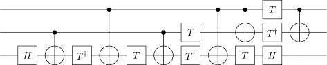
Figure 7: Standard decomposition of a Toffoli gate into $1-$ and $2-$ qubit gates.

The decomposition of a Toffoli gate as implemented in the qiskit framework is depicted in Figure 7. A complete example using qprof to profile the default Toffoli gate decomposition in qiskit is shown in Figure 8.

⬇

from qiskit import QuantumCircuit

from qprof import profile

# Circuit construction

circuit = QuantumCircuit(3, name=”one_ccx_circuit”)

circuit.ccx(0, 1, 2)

# Profiling

gate_times = {

”u1”: 0, ”u2”: 10, ”u3”: 30, ”u”: 30, ”cx”: 300

}

gprof_output = profile(circuit, gate_times, ”gprof”,

include_native_gates=True)

with open(”out.qprof”, ”w”) as f:

f.write(gprof_output)

Figure 8: Python code needed to use qprof on the Toffoli gate implementation and save the profiler report in a gprof-compatible format in a file named out.qprof.

The output of qprof, which is here in a gprof format with some slight adaptations as discussed in Section II.5, can then be analysed. For the sake of readability and brevity, the full gprof-compatible profiler report will not be included verbatim in this paper and will rather be visualised using the gprof2dot tool that allows representing gprof reports as call-graphs. The call-graph obtained from the report generated in Figure 8 is depicted in Figure 9.

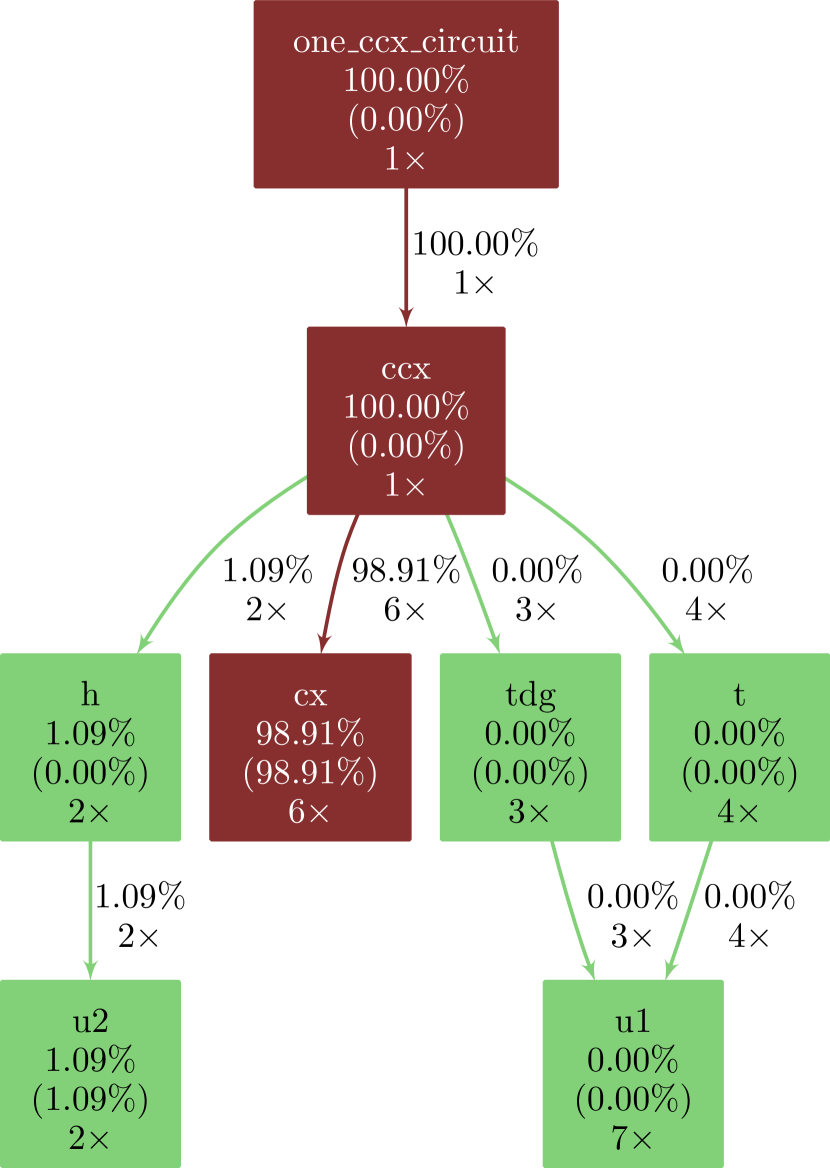
Figure 9: Call-graph for the Toffoli gate implementation. Quantum gates included in the gate_times variable (here u, u1, u2, u3 and cx) are considered as native gates. Only native gates have a non-zero self-time as they are the only gates that are really executed on the hardware.

From the call-graph depicted in Figure 9, it is clear that the cost of a Toffoli gate comes from its 6 controlled-$X$ gates, that account for more than $98\%$ of the total execution time. It is also interesting to note that the $T$ gate, known to be very costly when error-correction is needed, is ”free” on IBM chips when error-correction is not needed as it is equivalent to a phase change.

III.2 Grover’s algorithm

The Toffoli gate is a good example to start and understand the meaning of qprof’s output but the end goal of qprof is to be able to profile large and complex quantum circuits. A good first candidate to show how qprof performs on a more complex circuit is Grover’s algorithm.

In this example we use Grover’s algorithm on four qubits to find the three quantum states that verify the following formula:

$$(q_{0}\lor\neg q_{1})\land(\neg q_{2}\land q_{3}).$$ (1)

The only three $4$-qubit quantum states verifying Equation 1 are $\left|0001\right\rangle$, $\left|1001\right\rangle$ and $\left|1101\right\rangle$, $q_{0}$ being the left-most qubit in the bra-ket notation.

The code needed to generate the gprof-compatible output for Grover’s algorithm with the oracle presented in Equation 1 is given in Figure 10. The resulting call-graph, included in Figure 11, clearly shows that the controlled-$X$ gate is still the major contributor to execution time. But this time, contrarily to the Toffoli example shown in Section III.1, the controlled-$X$ gate is called by three different subroutines that all contribute significantly to the overall cost: c3z, ccz and mcx.

Thanks to qprof it is now easy to understand the subroutines that contribute the most to the total execution time. More importantly, the qprof-compatible report and the call-graph representation gives very insightful information about subroutines calls that are crucial for circuit optimisation. Such information can be used to weight the impact of a given optimisation and then decide whether or not it is worth applying it.

For example, knowing that the ccz subroutine takes $18.61\%$ of the total time, it is easy to deduce that a $20\%$ improvement in the implementation of ccz will translate into a tiny $\frac{18.61\%}{5}=3.72\%$ improvement to the overall execution time, which might not be worth the effort. On the other hand, optimising the c3z subroutine to reduce its execution time by $20\%$ improves the overall running time by $9.22\%$, which is nearly $10\%$ and might be an interesting optimisation target. Finally, the call-graph visualisation conveys clearly the information that the cx gate is the most costly subroutine of the Grover’s circuit, meaning that even a slight optimisation of the cx execution time will have a high impact on the overall implementation run-time.

⬇

from qiskit.algorithms import (

AmplificationProblem, Grover

)

from qiskit.circuit.library import PhaseOracle

from qprof import profile

# Circuit construction

oracle = PhaseOracle(”(v0 | ~v1) & (~v2 & v3)”)

problem = AmplificationProblem(

oracle, is_good_state=oracle.evaluate_bitstring

)

grover = Grover(iterations=1)

circuit = grover.construct_circuit(problem)

# Profile

gate_times = {

”u1”: 0, ”u2”: 10, ”u3”: 30, ”u”: 30, ”cx”: 300

}

gprof_output = profile(circuit, gate_times, ”gprof”,

include_native_gates=True)

with open(”out.qprof”, ”w”) as f:

f.write(gprof_output)

Figure 10: Python code needed to use qprof on the Grover implementation and save the profiler report in a gprof-compatible format in a file named out.qprof.

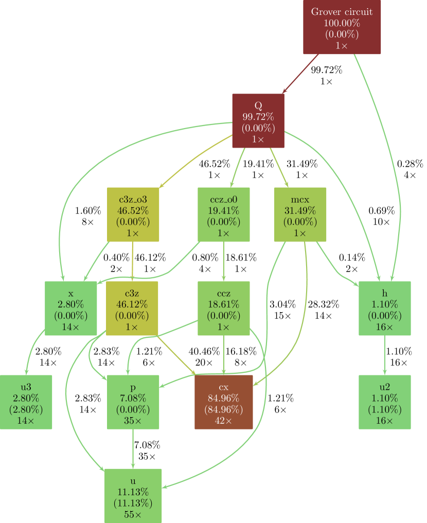
Figure 11: Call-graph for the Grover’s algorithm implementation. Quantum gates included in the gate_times variable (here u, u1, u2, u3 and cx) are considered as native gates. Only native gates have a non-zero self-time as they are the only gates that are really executed on the hardware. Some percentages might not add up to exactly $100\%$ due to rounding errors.

III.3 Quantum wave equation solver

Finally, we include in this paper a more complex example that has been implemented in a previous work with myQLM, a quantum computing framework maintained by Atos. The code used to generate the benchmarked quantum program is available at https://gitlab.com/cerfacs/qaths/ and is explained in Suau et al. (2021).

⬇

from qaths.applications.wave_equation.evolve_1D_dirichlet import evolve_1d_dirichlet

from qaths.applications.wave_equation.linking_sets.arithmetic_adder import get_linking_set as arith_linking_set

from qprof import profile

# Circuit generation

time = 0.1

discretisation_size = 2 ** 10

epsilon = 1e-3

trotter_order = 1

routine = evolve_1d_dirichlet(time, discretisation_size, epsilon, trotter_order)

# Gate execution time definition

G = {”u1”: 0, ”u2”: 89, ”u3”: 178, ”cx”: 930}

gate_times = {

”cu1”: 2 * G[”cx”] + 2 * G[”u1”],

”cu2”: 2 * G[”cx”] + 2 * G[”u3”],

”X”: G[”u3”],

”H”: G[”u2”],

”CNOT”: G[”cx”],

”CCNOT”: 6 * G[”cx”] + 2 * G[”u2”] + 7 * G[”u1”],

”CH”: 2 * G[”cx”] + 2 * G[”u3”],

”PH”: 3 * G[”u1”] + 2 * G[”cx”],

”CPH”: 3 * G[”u1”] + 2 * G[”cx”],

”CCPH”: None,

}

gate_times[”CCPH”] = 3 * gate_times[”CPH”] + 2 * gate_times[”CCNOT”]

gate_times[”CCCNOT”] = 6 * gate_times[”CCNOT”] + 2 * gate_times[”cu2”] + 7 * gate_times[”cu1”]

# Profiling

gprof_output = profile(

routine,

gate_times,

linking_set=arith_linking_set(discretisation_size),

exporter=”gprof”,

)

with open(”out.qprof”, ”w”) as f:

f.write(gprof_output)

Figure 12: Python code needed to use qprof with the QatHS library, on top of myQLM, and save the profiler report in a gprof-compatible format in a file named out.qprof.

This example demonstrates that, as can be seen in Figure 12, qprof interface stays nearly the same even though the framework used is now completely different. The only exceptions are some additional parameters (such as linking_set in Figure 12) that are directly forwarded to the framework plugin used and additional gate definitions in the gate_times data structure because of the way gate decomposition is handled in myQLM.

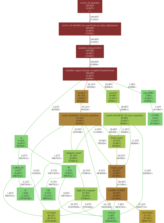
Figure 13: Call-graph of the quantum wave equation solver. Nodes (i.e. quantum routines) that account for less than $0.5\%$ of the total execution time are not plotted. Edges (i.e. subroutine calls) that account for $0.1\%$ or less of the total execution time are also discarded for readability purposes.

The call graph obtained by running Figure 12 is reproduced in Figure 13. In order for the call-graph to be readable on a paper format, some subroutines and calls (i.e. nodes and edges respectively) have been discarded from the graphical representation. The call-graph clearly shows that most of the execution time is spent in the oracle implementation. Moreover, (multi-)controlled-$X$ gates are the major contributors to the total execution time.

IV Conclusion

In this paper we introduced an open-source and, to the best of our knowledge, novel library that is able to generate profiling reports in well-known formats from a quantum circuit implementation. Our library is able to natively read quantum circuits from multiple frameworks – currently Qiskit and myQLM – and can be easily extended to support more quantum computing libraries. It generates consistent reports independently of the underlying framework used. qprof opens new optimisation opportunities for quantum scientists and programmers by allowing them to view their quantum circuit implementation in a well-known, familiar, synthetic and visual representation. In this paper, we first presented the main concepts used in the internals of qprof and required to make it as extendable as possible: the plugin interface used to wrap different quantum computing frameworks, the call-graph data structure and finally the different native exporters. Then, we used qprof on three different quantum circuit implementations of increasing complexity to demonstrate its features: simplicity of use, adaptability, consistency of the interface and efficiency.

In the future, we plan to extend the set of supported quantum computing frameworks. The number of exporters can also be improved to handle different output formats such as a perf_event Foundation (2020b) compatible format, allowing to easily use new visualisations such as flame graphs Gregg (2016).

Supplementary material

The qprof tool is available at https://gitlab.com/qcomputing/qprof/qprof.

- (1)
- Aaronson and Gottesman (2004) Scott Aaronson and Daniel Gottesman. 2004. Improved simulation of stabilizer circuits. Physical Review A 70, 5 (Nov 2004). https://doi.org/10.1103/physreva.70.052328
- Abraham et al. (2019) Héctor Abraham, AduOffei, Rochisha Agarwal, Ismail Yunus Akhalwaya, Gadi Aleksandrowicz, Thomas Alexander, Matthew Amy, Eli Arbel, Arijit02, Abraham Asfaw, Artur Avkhadiev, Carlos Azaustre, AzizNgoueya, Abhik Banerjee, Aman Bansal, et al. 2019. Qiskit: An Open-source Framework for Quantum Computing. (2019). https://doi.org/10.5281/zenodo.2562110
- Bae et al. (2020) J.-H. Bae, Paul M. Alsing, Doyeol Ahn, and Warner A. Miller. 2020. Quantum circuit optimization using quantum Karnaugh map. Scientific Reports 10, 1 (Sept. 2020). https://doi.org/10.1038/s41598-020-72469-7
- Bravyi et al. (2021) Sergey Bravyi, Sarah Sheldon, Abhinav Kandala, David C. Mckay, and Jay M. Gambetta. 2021. Mitigating measurement errors in multiqubit experiments. Physical Review A 103, 4 (Apr 2021). https://doi.org/10.1103/physreva.103.042605
- Childs et al. (2018) Andrew M. Childs, Dmitri Maslov, Yunseong Nam, Neil J. Ross, and Yuan Su. 2018. Toward the first quantum simulation with quantum speedup. Proceedings of the National Academy of Sciences 115, 38 (Sep 2018), 9456–9461. https://doi.org/10.1073/pnas.1801723115
- Cirq Developers (2021) Cirq Developers. 2021. Cirq. (2021). https://doi.org/10.5281/ZENODO.4062499
- Computing (2021) Rigetti Computing. 2021. PyQuil documentation. (2021). https://pyquil-docs.rigetti.com/en/stable/
- Cross et al. (2016) Andrew W Cross, Easwar Magesan, Lev S Bishop, John A Smolin, and Jay M Gambetta. 2016. Scalable randomised benchmarking of non-Clifford gates. npj Quantum Information 2, 1 (April 2016). https://doi.org/10.1038/npjqi.2016.12
- Earnest et al. (2021) Nathan Earnest, Caroline Tornow, and Daniel J. Egger. 2021. Pulse-efficient circuit transpilation for quantum applications on cross-resonance-based hardware. (2021). arXiv:quant-ph/2105.01063
- Emerson et al. (2005) Joseph Emerson, Robert Alicki, and Karol Życzkowski. 2005. Scalable noise estimation with random unitary operators. Journal of Optics B: Quantum and Semiclassical Optics 7, 10 (Sep 2005), S347–S352. https://doi.org/10.1088/1464-4266/7/10/021
- Foundation (2020a) Free Software Foundation. 2020a. GNU gprof. (2020). https://sourceware.org/binutils/docs/gprof/index.html
- Foundation (2020b) The Linux Foundation. 2020b. perf_event tutorial. (2020). https://perf.wiki.kernel.org
- Fösel et al. (2021) Thomas Fösel, Murphy Yuezhen Niu, Florian Marquardt, and Li Li. 2021. Quantum circuit optimization with deep reinforcement learning. (2021). arXiv:quant-ph/2103.07585
- Gambetta et al. (2012) Jay M. Gambetta, A. D. Córcoles, S. T. Merkel, B. R. Johnson, John A. Smolin, Jerry M. Chow, Colm A. Ryan, Chad Rigetti, S. Poletto, Thomas A. Ohki, and et al. 2012. Characterization of Addressability by Simultaneous Randomized Benchmarking. Physical Review Letters 109, 24 (Dec 2012). https://doi.org/10.1103/physrevlett.109.240504
- Gidney (2021) Craig Gidney. 2021. Stim: a fast stabilizer circuit simulator. (2021). arXiv:quant-ph/2103.02202
- Gokhale et al. (2020) Pranav Gokhale, Ali Javadi-Abhari, Nathan Earnest, Yunong Shi, and Frederic T. Chong. 2020. Optimized Quantum Compilation for Near-Term Algorithms with OpenPulse. (2020). arXiv:quant-ph/2004.11205
- Graham et al. (1982) Susan L. Graham, Peter B. Kessler, and Marshall K. Mckusick. 1982. Gprof: A Call Graph Execution Profiler. SIGPLAN Not. 17, 6 (June 1982), 120–126. https://doi.org/10.1145/872726.806987
- Gregg (2016) Brendan Gregg. 2016. The Flame Graph. Commun. ACM 59, 6 (May 2016), 48–57. https://doi.org/10.1145/2909476
- Iten et al. (2019) Raban Iten, Romain Moyard, Tony Metger, David Sutter, and Stefan Woerner. 2019. Exact and practical pattern matching for quantum circuit optimization. Article arXiv:1909.05270 (Sept. 2019), arXiv:1909.05270 pages. arXiv:quant-ph/1909.05270
- Knill et al. (2008) E. Knill, D. Leibfried, R. Reichle, J. Britton, R. B. Blakestad, J. D. Jost, C. Langer, R. Ozeri, S. Seidelin, and D. J. Wineland. 2008. Randomized benchmarking of quantum gates. Physical Review A 77, 1 (Jan 2008). https://doi.org/10.1103/physreva.77.012307
- LaRose et al. (2020) Ryan LaRose, Andrea Mari, Peter J. Karalekas, Nathan Shammah, and William J. Zeng. 2020. Mitiq: A software package for error mitigation on noisy quantum computers. (2020). arXiv:quant-ph/2009.04417
- Maslov et al. (2008) D. Maslov, G.W. Dueck, D.M. Miller, and C. Negrevergne. 2008. Quantum Circuit Simplification and Level Compaction. IEEE Transactions on Computer-Aided Design of Integrated Circuits and Systems 27, 3 (Mar 2008), 436–444. https://doi.org/10.1109/tcad.2007.911334
- McKay et al. (2019) David C. McKay, Sarah Sheldon, John A. Smolin, Jerry M. Chow, and Jay M. Gambetta. 2019. Three-Qubit Randomized Benchmarking. Phys. Rev. Lett. 122 (May 2019), 200502. Issue 20. https://doi.org/10.1103/PhysRevLett.122.200502
- Nam et al. (2018) Yunseong Nam, Neil J. Ross, Yuan Su, Andrew M. Childs, and Dmitri Maslov. 2018. Automated optimization of large quantum circuits with continuous parameters. npj Quantum Information 4, 1 (May 2018). https://doi.org/10.1038/s41534-018-0072-4
- Schollwöck (2011) Ulrich Schollwöck. 2011. The density-matrix renormalization group in the age of matrix product states. Annals of Physics 326, 1 (Jan 2011), 96–192. https://doi.org/10.1016/j.aop.2010.09.012
- Shi et al. (2019) Yunong Shi, Nelson Leung, Pranav Gokhale, Zane Rossi, David I. Schuster, Henry Hoffmann, and Frederic T. Chong. 2019. Optimized Compilation of Aggregated Instructions for Realistic Quantum Computers. In Proceedings of the Twenty-Fourth International Conference on Architectural Support for Programming Languages and Operating Systems (ASPLOS ’19). Association for Computing Machinery, New York, NY, USA, 1031–1044. https://doi.org/10.1145/3297858.3304018
- Suau et al. (2021) Adrien Suau, Gabriel Staffelbach, and Henri Calandra. 2021. Practical Quantum Computing: Solving the Wave Equation Using a Quantum Approach. ACM Transactions on Quantum Computing 2, 1, Article 2 (2 2021), 35 pages. https://doi.org/10.1145/3430030 arXiv:quant-ph/2003.12458
- team (2021a) Atos Quantum Computing team. 2021a. myQLM documentation. (2021). https://myqlm.github.io/
- team (2021b) Microsoft Quantum team. 2021b. The Q# User Guide. (2021). https://docs.microsoft.com/en-us/azure/quantum/user-guide/
- Vidal (2003) Guifré Vidal. 2003. Efficient Classical Simulation of Slightly Entangled Quantum Computations. Physical Review Letters 91, 14 (Oct 2003). https://doi.org/10.1103/physrevlett.91.147902