Quantum diffusion map for nonlinear dimensionality reduction

Abstract

Inspired by random walk on graphs, diffusion map (DM) is a class of unsupervised machine learning that offers automatic identification of low-dimensional data structure hidden in a high-dimensional dataset. In recent years, among its many applications, DM has been successfully applied to discover relevant order parameters in many-body systems, enabling automatic classification of quantum phases of matter. However, classical DM algorithm is computationally prohibitive for a large dataset, and any reduction of the time complexity would be desirable. With a quantum computational speedup in mind, we propose a quantum algorithm for DM, termed quantum diffusion map (qDM). Our qDM takes as an input $N$ classical data vectors, performs an eigen-decomposition of the Markov transition matrix in time $O(\log^{3}N)$, and classically constructs the diffusion map via the readout (tomography) of the eigenvectors, giving a total expected runtime proportional to $N^{2}\text{polylog}\,N$. Lastly, quantum subroutines in qDM for constructing a Markov transition matrix, and for analyzing its spectral properties can also be useful for other random walk-based algorithms.

I INTRODUCTION

Discovering statistical structure in high-dimensional data is essential for data-driven science and engineering. Advances in unsupervised machine learning offer a plethora of alternatives to automatically search for low-dimensional structure of data lying in a high-dimensional space. Many of these approaches involve dimensionality reduction. Classic approach is the principal component analysis (PCA), which projects high-dimensional data onto a low-dimensional linear space spanned by a set of orthonormal bases, whose directions capture significant data variations. More compelling approach enables automatic searches for a low-dimensional data manifold embedded in a high-dimensional space. Well-known manifold learning algorithms include Isomap [1], Laplacian eigenmaps [2], uniform manifold approximation and projection (UMAP) [3], nonlinear PCA [4], t-distributed stochastic neighbor embedding (t-SNE) [5], and diffusion map (DM) [6, 7, 8], which is the focus of this paper. Inspired by appealing features of random walk on graphs, DM and its variants have received increasing attention for data visualization in bioinformatics [9, 10]. DM has also recently been sucessfully applied to provide automatic classification of topological phases of matter, and offers automatic identification of quantum phase transitions in many-body systems [11, 12, 13, 14, 15, 16].

Most dimensionality reduction methods require the computation of singular value decomposition (SVD) of a matrix constructed from a collection of high-dimensional data points. For a matrix of size, say, $N\times d$, where $N$ is the number of data points and $d$ is the dimensionality of each data vector (assumed to be smaller than $N$), the computational cost of SVD typically grows with the number of data points as $O(N^{3})$. Thus, classical dimensionality reduction can be computationally prohibitive for a large data sample. However, under moderate assumptions of accessibility to certain features of full-scale quantum computers, matrix exponentiation-based quantum algorithms have been proposed to perform SVD more efficiently [17]. In particular, assuming efficient encoding of classical data to quantum information and accessibility to appropriate quantum RAM, quantum singular value decomposition (qSVD) algorithm’s runtime for many non-sparse low-rank Hermitian matrices is $O(\text{polylog}\,N)$, which is exponentially faster than the classical counterpart and can be extended to non-square matrices. A classic quantum algorithm for dimensionality reduction with quantum computational speedup is quantum principal component analysis (qPCA), which exploits matrix exponentiation tricks as in qSVD [18]. More recently, quantum algorithms with quantum advantage for nonlinear dimensionality reduction with nonlinear kernel [19] and cluster identification based on spectral graph theory have also been proposed [20, 21, 22].

With a quantum computational speedup for dimensionality reduction in mind, we propose a quantum algorithm for unsupervised manifold learning called quantum diffusion map (qDM). Under mild assumptions of appropriate oracles, qDM has an expected runtime of roughly $\kappa_{D}^{0.625}N^{2}\mathrm{polylog}\,N$ where $N$ is the number of data points and $\kappa_{D}$ is the condition number of the degree matrix (see Theorem 1 and Lemma 1 for the precise statement), as opposed to $O(N^{3})$ in classical DM. Although $\kappa_{D}$ depends strongly on the data structure and can take the value $N$ in the worst case, such worst-case is highly atypical for well structured dataset, in which $\kappa_{D}=O(1)$. Without the final readout step, our qDM algorithm prepares all necessary components for constructing diffusion map in $O(\kappa_{D}^{0.625}\log^{3}N)$ time.

Although the backbone of DM is a graph-based dimensionality reduction method, the procedure is different from other spectral graph methods. Namely, rather than working with the data-induced graph Laplacian as in Laplacian eigenmaps or in spectral clustering, DM involves Markov transition matrix that defines random walks on a data-induced graph. Therefore, recipes for qDM dimensionality reduction are different from the recently proposed quantum spectral clustering [20, 21], mainly in the efficient construction of the degree matrix, which was mentioned as not efficiently accessible [21]. Our algorithm also exploits the coherent state encoding scheme, initially proposed in Ref. [23], to provide an exact quantum encoding of classical Gaussian kernel. This is in contrast to the quantum kernel principle component analysis (qKPCA) [19] for dimensionality reduction, which only encodes nonlinear kernel approximately.

The paper is organized as follows. Section II provides necessary ingredients to understand classical diffusion map and its runtime. Section III introduces quantum subroutines for qDM, which is then discussed in details in Section IV and V. qDM runtime complexity appears in Section VI. We conclude with the discussion and outlook in Section VII. Additional details on the algorithmic complexity and the subroutines for qDM are provided in Appendix A and B.

II Classical diffusion map for dimensionality reduction

Given a set of $N$ data vectors $X\equiv\quantity{\bm{x}^{(i)}}_{i=0}^{N-1}$, in which each data vector has $d$ features (i.e. $\bm{x}^{(i)}\in\mathbb{R}^{d}$), unsupervised machine learning seeks to identify the structure of data distribution in a high-dimensional ($d\gg 1$) space. When the data distribution has a highly nonlinear structure, classic linear approach such as PCA fails. Rather than using mere Euclidean distance as a similarity measure between data points, manifold learning approach assigns the connectivity among data points in their neighborhood as a proxy for proximity between points; e.g., points on a toroidal helix embedded in 3 dimensions with equal Euclidean distance can have different geodesic distances on a manifold (different similarity), see Fig. 1 (top). This approach allows one to perform a nonlinear dimensionality reduction by assigning an appropriate function that maps a high-dimensional data point into a relevant lower-dimensional Euclidean space embedding, while encapsulating the notion of proximity in high dimensions based on neighborhood connectivity.

Neighborhood connectivity leads to the development of graph-based manifold learning approach, where one can assign a vertex $i$ to a data vector $\bm{x}^{(i)}$ and assign an edge between a pair of data points that are considered to be neighbors. Isomap [1] and Laplacian eigenmaps [2] are among the first graph-based manifold learning algorithms, where relevant low-dimensional data embedding can be extracted from eigen-decomposition of data-induced graph Laplacian matrix.

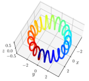
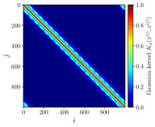
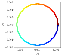
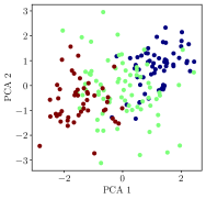
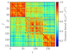
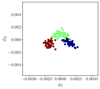
Figure 1: The application of classical DM for nonlinear dimensionality reduction: (top) to identify the proximity structure of data points distributed as a toroidal helix in 3 dimensions, and (bottom) to reveal the proximity structure of 13 chemical components’ concentrations of 178 wines ($d=13,N=178$) derived from 3 different cultivars grown in the same region in Italy, taken from the WINE dataset in [24]. In a toroidal helix data (top left), color variation signifies difference in the geodesic distance between points on a one-dimensional manifold. The Gaussian kernel with $\sigma=1$ of (1) shows the neighborhood connectivity has a local, periodic structure (top middle). The dimensionality reduction (top right) into the first two components ($m=2$) of the DM in (5) reveals a one-dimensional structure with an appropriate notion of geodesic distance (see color variations). In WINE dataset, wines grown from 3 different cultivars are labeled in 3 different colors (red, green, blue). Projecting the 13 data features (chemical concentrations) of all wines into the first two principal components using PCA does not suffice to distinguish the 3 types (bottom left). However, with the Gaussian kernel with $\sigma=50$ (bottom middle), DM with two bases ($m=2$) can reveal quite a clear distinction between types (bottom right). In addition, the proximity structure also suggests that the green type has its chemical components closer to those of the other two types. In both dataset, we use $t=1$ in the DM. Thus, random walk on data-induced graphs can reveal salient low-dimensional data structure within just a one-step walk, provided $\sigma$ is chosen appropriately.

II.1 Diffusion map in a nutshell

In diffusion map (DM), the similarity matrix between a pair of data vectors, or equivalently the weighted edge between a pair of graph vertices, is often taken to be a Gaussian kernel:

$$W_{ij}\equiv K_{\sigma}\quantity({\bf\it x}^{(i)},{\bf\it x}^{(j)})=\exp\quantity(-\frac{\norm{{\bf\it x}^{(i)}-{\bf\it x}^{(j)}}_{2}^{2}}{2\sigma}),$$ (1)

where the adjustable parameter $\sigma$, called the bandwidth, sets the scale of neighborhood. Two points whose squared distance exceed this bandwidth contribute exponentially little to the weighted edge, suggesting that these two points are far away from being a neighbor in its original feature space. Given a graph with weighted edges $W_{ij}$’s, DM assigns a discrete-time random walk on a data-induced graph, where the Markov transition probability from vertex $i$ to $j$ is given by the normalized weighted edge,

$$P_{ij}=\frac{W_{ij}}{\sum_{j=0}^{N-1}W_{ij}}.$$ (2)

One can compactly compute the Markov transition matrix $P$ from the (weighted) adjacency matrix $W$, and the degree matrix $D\equiv\text{diag}\{d_{i}\}_{i=0}^{N-1}$ where $d_{i}\equiv\sum_{j=0}^{N-1}W_{ij}$ by

$$P=D^{-1}W.$$ (3)

The notion of proximity based on graph connectivity can be characterized by how fast random walkers on a graph starting at different data points visit each other. One expects that two points that are connected by multiple paths should be near; whereas two points that are sparsely connected should lie far from each other. In fact, it can be shown that [8] the proper distance function, called diffusion distance, between two points $\bm{x}^{(i)}$ and $\bm{x}^{(j)}$ after a $t$-step random walk is given by

$$\operatorname{Dist}_{t}^{2}\left(\bm{x}^{(i)},\bm{x}^{(j)}\right)=\sum_{k=0}^{N-1}\frac{\left[\left(P^{t}\right)_{ik}-\left(P^{t}\right)_{jk}\right]^{2}}{u_{0}\left(\bm{x}^{(k)}\right)},$$ (4)

where $u_{0}$ is the left eigenvector with eigenvalue $\lambda_{0}=1$ of $P$ and $u_{0}\left(\bm{x}^{(k)}\right)$ denotes the $k^{\textrm{th}}$ coordinate of $u_{0}$.

Before obtaining a relevant lower-dimensional Euclidean space representation of the original data point $\bm{x}^{(i)}$, we first note the following important identity. Define the diffusion map with $m$ bases as

$${\bf\it\phi}_{t,m}\quantity({\bf\it x}^{(i)})=\begin{pmatrix}\lambda_{1}^{t}v_{1}\left({\bf\it x}^{(i)}\right)\\ \vdots\\ \lambda_{m}^{t}v_{m}\left({\bf\it x}^{(i)}\right)\end{pmatrix},$$ (5)

where $v_{i}$ is the right eigenvector of $P$ with eigenvalue $\lambda_{i}$, $v_{i}\left(\bm{x}^{(j)}\right)$ denotes the $j^{\textrm{th}}$ coordinate of $v_{i}$, and the eigenvalues are ordered such that $\lambda_{0}=1>\lambda_{1}\geq\lambda_{2}\geq\ldots\geq\lambda_{N-1}\geq 0$ assuming no degeneracy in the largest eigenvalue (which is always possible given $\sigma$ is sufficiently large). Note that $\lambda_{0}=1$ is always the eigenvalue of a Markov transition matrix $P$ with a normalized eigenvector $\matrixquantity(1&\cdots&1)^{T}/N$, corresponding to the stationary uniform distribution over all vertices. Then, the diffusion distance (4) can be exactly computed from the Euclidean representation in (5) with $m=N-1$ bases [8];

$$\operatorname{Dist}_{t}^{2}\left(\bm{x}^{(i)},\bm{x}^{(j)}\right)=\norm{{\bf\it\phi}_{t,N-1}\quantity({\bf\it x}^{(i)})-{\bf\it\phi}_{t,N-1}\quantity({\bf\it x}^{(j)})}_{2}^{2}.$$ (6)

The above equality states that the distance in the diffusion space (based on graph connectivity) is identical to the Euclidean embedding distance (induced by the diffusion map). Thus, the notion of proximity between data points from its graph connectivity can be simply computed from the Euclidean embedding by the diffusion map (5).

What about dimensionality reduction? Since $P$ is a Markov transition matrix, its eigenvalues are $\lambda_{0}=1\geq\lambda_{1}\geq\lambda_{2}\geq\ldots\geq\lambda_{N-1}\geq 0.$ Bases in (5) with low-lying eigenvalues are then exponentially suppressed as $t$-step increases. In the long-time limit, dimensionality reduction thus naturally arises in DM. One may take the number of bases $m$ in (5) corresponding to the number of top eigenvalues of $P$, and still obtain meaningful low-dimensional Euclidean representation of points in the diffusion space. In practice, for the purpose of visualization, taking $m=2\ll d$ is a drastic dimensionality reduction, yet DM with such small number of bases can yield insights into the approximate proximity of data in the original high-dimensional space, see Fig. 1. Using DM (5) to extract low-dimensional data representation that approximately preserves the notion of distance from neighborhood connectivity in the original high-dimensional space is also the first step towards data clustering algorithms. Namely, one may employ standard clustering algorithms, such as k-means algorithm, on the low-dimensional outputs of the DM without suffering from the curse of dimensionality problem.

II.2 Time complexity of classical diffusion map

Numerical recipes to obtain nonlinear dimensionality reduction or manifold learning in classical DM consists of 4 steps:

1. Construct the data-induced similarity matrix (weighted adjacency matrix) $W$ from (1)

2. Construct the Markov transition matrix $P$ from (3); i.e. $P=D^{-1}W$

3. Compute the eigen-decomposition of $P$

4. Construct the diffusion map (5)

We now discuss the time complexity for each step as a function of the number of data points $N$. Assuming the Gaussian kernel function (1), the weighted adjacency matrix $W$ is symmetric. The number of the elements that the algorithm needs to calculate is then $\sum_{i=1}^{N}i=(N^{2}+N)/2$. Therefore, the time complexity of calculating the kernel matrix in step 1 is $O\left(N^{2}\right)$.

For step 2, the calculation of $P$ involves normalizing each row of $W$ as in (2). Numerical computation of the normalization factor, which is simply the summation, takes the time $O(N)$. Then normalizing each row costs another $O(N)$. Applying these procedures over the $N\times N$ matrix thus yields the time cost $O(N^{2})+O(N^{2})$. Hence, the time complexity for computing $P$ is $O(N^{2})$.

In step 3, the time cost stems from finding $\{v_{i}\}$ and $\{\lambda_{i}\}$ of $P$, using singular value decomposition (SVD), which can be applied to any non-squared matrices. This algorithm comprises two steps [25]. The first step is to use Householder transformations to reduce $P$ to a bidiagonal form. Then the QR algorithm is applied to find singular values. The time complexity of these two steps combined is $O(N^{3})$.

The last step is computing the diffusion map $\bm{\phi}$ according to (5), which involves the multiplication of $\lambda_{i}^{t}$ with its corresponding right eigenvector $v_{i}$. Although we might not need to perform the multiplication for all $N-1$ right eigenvectors as some $\lambda_{i}^{t}$ maybe negligible in the long-time limit, we consider the worst case scenario where all $N-1$ eigenvectors are required. With the length of each vector being $N$, the time cost is $O(N^{2}-N)$ for computing $\bm{\phi}$ and thus the time complexity for this step is $O(N^{2})$.

Combining all the steps above, which is implemented in sequence, classical DM has a time complexity of $O(N^{2})+O(N^{2})+O(N^{3})+O(N^{2})$ leading to an overall time complexity that scales as $O(N^{3})$. Note here that the time complexity is primarily dominated by the eigen-decomposition algorithm, which is subjected to change if a different algorithm is chosen in the implementation. In fact, this dominating complexity of $O(N^{3})$ from eigen-decomposition urges for the development of quantum algorithms to achieve a quantum computational speedup, which we discuss next.

III Quantum diffusion map roadmap

In this section, we first give an outline of qDM algorithm summarized in Fig. 2. Then we proceed with classical to quantum data encoding, and the construction of the kernel matrix in Sec. III.1 and Sec. III.2, respectively. Constructing the Markov transition matrix and extracting the relevant eigen-decomposition are not straightforward, and will be discussed in the following Sec. IV and Sec. V, respectively.

From now on, we will focus on the case where the weighted adjacency matrix is the Gaussian kernel matrix, so that $W=K$. To reduce the dominating complexity in the construction of the diffusion map, we first turn to the idea of quantum mechanically encoding the (normalized) kernel matrix a density matrix $\hat{K}$ without explicitly evaluating each matrix element. Using the fact that the Gaussian kernel (1) is the inner product of canonical coherent states, this can be done in $O(\log N)$ time assuming quantum random access memory (qRAM) by exploiting “quantum parallelism”, the ability to query data in superposition. We further discuss the assumption of qRAM in Appendix B.1.

To construct the transition matrix, our algorithm uses as subroutines density matrix exponentiation [18], quantum matrix algebra toolbox (QMAT) [26], and quantum matrix inversion [27, 28]. While it is straightforward to classically compute the degree matrix $D$ given elements of $K$, here we do not have direct access to elements of the density matrix $\hat{K}$ without performing full tomography. Instead, we compute $D$ via the identity

$$D=(K{\mathbbm{1}})\odot I,$$ (7)

where $\odot$ is element-wise multiplication also known as Hadamard product, ${\mathbbm{1}}$ is the all-ones matrix, and $I$ is the identity matrix. Such matrix arithmetics can be done in the QMAT framework given the exponential of the relevant matrices either by density matrix exponentiation for $\hat{K}$, or Hamiltonian simulation to exponentiate sparse matrices [29]. We then use quantum phase estimation (QPE) to construct the inverse square-root of $D$ (akin to the HHL algorithm [27]). Then the (right) eigenvectors and eigenvalues of the transition matrix $P\equiv D^{-1}K$ can be obtained from the eigen-decomposition (via another QPE) of the symmetrized transition matrix $S\equiv D^{-1/2}KD^{-1/2}$. The diffusion map is then constructed classically. The time complexity is given in Section VI.

Figure 2: The roadmap for quantum diffusion map algorithm, which also enables an efficient construction of the transition matrix for generating random walk on graphs as a byproduct. Note that we do not perform the eigen-decomposition of the transition matrix directly since quantum phase estimation (QPE) only eigen-decomposes symmetric matrices. Nevertheless the eigenpairs of the original transition matrix can be reconstructed from those of the symmetrized transition matrix.

III.1 Quantum state encoding into coherent states

By the fact that the Gaussian kernel arises naturally as the inner product of coherent states, ref. [23] proposed encoding classical data into multi-mode coherent states

$${{\bf\it x}}^{(i)}\mapsto\ket{{\bf\it x}^{(i)}}=\bigotimes_{p=0}^{d-1}\ket{x_{p}^{(i)}},$$ (8)

where each single-mode coherent state $\ket{x_{p}^{(i)}}$ reprensents the $p^{\text{th}}$ feature of datum ${\bf\it x}^{(i)}$. In continuous-variable quantum systems, the canonical coherent states are states with minimal and equal uncertainties in both quadratures. They are displaced ground state of the harmonic oscillator, and can be realized, for example, as the state of classical electromagnetic radiation. A single-mode coherent state is defined as

$$\ket{x_{p}^{(i)}}=\exp(-\frac{\quantity(x_{p}^{(i)})^{2}}{2})\sum_{n=0}^{\infty}\frac{\quantity(x_{p}^{(i)})^{n}}{\sqrt{n!}}\ket{n},$$ (9)

where $\ket{n}$ is the $n^{th}$ eigenstate of the harmonic oscillator.

The inner product between two data vectors is the Gaussian kernel

$$\begin{split}\innerproduct{{\bf\it x}^{(i)}}{{\bf\it x}^{(j)}}&=\prod_{p=0}^{d-1}\innerproduct{x_{p}^{(i)}}{x_{p}^{(j)}}\\ &=\prod_{p=0}^{d-1}\exp(-\frac{\quantity(x_{p}^{(i)}-x_{p}^{(j)})^{2}}{2})\\ &=\exp(-\frac{\norm{{\bf\it x}^{(i)}-{\bf\it x}^{(j)}}_{2}^{2}}{2})=K\quantity({\bf\it x}^{(i)},{\bf\it x}^{(j)}).\end{split}$$ (10)

Here, we take $\sigma=1$ for simplicity (though $\sigma$ can be incorporated by a scaling factor during state encoding in classical pre-processing). Recall that we focus on the kernel matrix as the weight matrix, and thus we denote $K$ for describing the weight matrix $W$.

III.2 Kernel matrix

Now we exploit superposition access to the encoded data to implicitly evaluate the kernel matrix. This can be done efficiently assuming qRAM for instance [30, 31]. Calling the oracle with the state $\frac{1}{\sqrt{N}}\sum_{i=0}^{N-1}\ket{i}$ entangles the data vectors with their labels:

$$\ket{\psi}=\frac{1}{\sqrt{N}}\sum_{i=0}^{N-1}\ket{i}_{\mathrm{label}}\otimes\ket{{\bf\it x}^{(i)}}_{\mathrm{position}}.$$ (11)

The reduced density matrix of the label space is given by the partial trace over the position space:

$$\Tr_{\text{position}}(\outerproduct{\psi}{\psi}) =\frac{1}{N}\sum_{i,j=0}^{N-1}\innerproduct{{\bf\it x}^{(i)}}{{\bf\it x}^{(j)}}\outerproduct{i}{j}$$

$$=\frac{1}{N}\sum_{i,j=0}^{N-1}K\quantity({\bf\it x}^{(i)},{\bf\it x}^{(j)})\outerproduct{i}{j}$$

$$=\frac{K}{N}\equiv\hat{K},$$ (12)

where $\Tr(\hat{K})=\sum_{i=0}^{N-1}K\quantity({\bf\it x}^{(i)},{\bf\it x}^{(i)})=N$. Copies of $\hat{K}$ will be used to prepare the degree matrix and the transition matrix.

IV Quantum subroutine for constructing the transition matrix

In this section, we show that the degree matrix and its inverse, and consequently the transition matrix, can be obtained efficiently in a coherent fashion. In particular, if one can efficiently perform matrix multiplication and Hadamard product $\odot$ involving $\hat{K}$, then one can efficiently obtain the degree matrix according to (7). Such matrix arithmetics can be done in the QMAT framework [26] by first exponentiating the relevant (possibly non-Hermitian) matrices $A$ in the form $e^{iX_{i}(A)}$, where

$$X_{i}(A)=R_{i}\otimes A+R_{i}^{\dagger}\otimes A^{\dagger},$$ (13)

and

$$R_{1}=\outerproduct{0}{1}, R_{2}=\outerproduct{1}{2}, R_{3}=\outerproduct{0}{2},$$ (14)

are qutrit operators. Once one has the ability to apply, say, $e^{iX_{1}(A_{1})}$ and $e^{iX_{2}(A_{2})}$ (shuffling between $R_{i},i=1,2,3$ can be done by a simple permutation of the qutrit basis states), then using the commutation relation between $X_{1}(A_{1})$ and $X_{2}(A_{2})$ one can approximate $e^{iX_{3}(A_{3})}$ where $A_{3}$ is the result of the desired binary operation between $A_{1}$ and $A_{2}$.

IV.1 Exponential of degree matrix

To compute the degree matrix, we require QMAT subroutines for (i) matrix multiplication, (ii) tensor product, and (iii) Hadamard product. The latter two subroutines reduce to matrix multiplication as $A_{1}\otimes A_{2}=(A_{1}\otimes I)(I\otimes A_{2})$, and

$$\Xi(A_{1}\otimes A_{2})\Xi^{\dagger}=(A_{1}\odot A_{2})\otimes\outerproduct{0}{0},$$ (15)

where

$$\Xi=\sum_{i=0}^{N-1}\outerproduct{i}{i}\otimes\outerproduct{{\bf 0}}{i},$$ (16)

and $\ket{\bf 0}=\ket{0\cdots 0}$ [26]. The multiplication subroutine and its complexity is summarized in Appendix A.

Define the (rank-one) density matrix

$$\hat{\mathbbm{1}}\equiv\frac{1}{N}\sum_{i,j=0}^{N-1}\outerproduct{i}{j}=\frac{\mathbbm{1}}{N}.$$ (17)

If $e^{iX_{i}(\hat{K})\tau}$, $e^{iX_{i}(\hat{\mathbbm{1}})\tau}$, $e^{iX_{i}(\Xi)\tau}$ and $e^{iX_{i}(\Xi^{\dagger})\tau}$ can be constructed efficiently for some time $\tau$, then one can construct for a larger time $t$ (to be determined later for the purpose of phase estimation) the controlled-$e^{iX_{3}(D)t}$ unitary

$$\begin{split}e^{iX_{3}(\Xi(\hat{K}\hat{\mathbbm{1}}\otimes I)\Xi^{\dagger})t}&=e^{iX_{3}(D)t}\otimes\outerproduct{{\bf\it 0}}{{\bf\it 0}}+I\otimes(I-\outerproduct{{\bf\it 0}}{{\bf\it 0}})\\ &\equiv\mathcal{U}_{D}.\end{split}$$ (18)

The last register will be discarded in the inversion step.

Now we discuss an efficient construction of the unitary matrices required in the above procedure. $\Xi$ is sparse and thus can be exponentiated efficiently . For the kernel matrix $\hat{K}$ and $\hat{\mathbbm{1}}$ which are not sparse, we can use the technique of density matrix exponentiation with time cost of $O(\tau^{2}/\epsilon)$ with accuracy $\epsilon$ [18]. (Note that we cannot exponentiate $X_{i}(A)$ directly using this method since $X_{i}(A)$ is not a density matrix. However, since $R_{i}+R_{i}^{\dagger}=\outerproduct{+_{i}}{+_{i}}-\outerproduct{-_{i}}{-_{i}}$, where $\ket{\pm_{i}}$ are the $\pm 1$-eigenvectors of $R_{i}+R_{i}^{\dagger}$, we can separately exponentiate $\outerproduct{\pm_{i}}{\pm_{i}}\otimes A$ with the time parameter $\pm\tau$ respectively and concatenate them to obtain the desired unitary operator.) Hence, $e^{iX_{3}(\hat{K}\hat{\mathbbm{1}})\tau}$ and automatically $e^{iX_{3}((\hat{K}\hat{\mathbbm{1}})\otimes I)\tau}$ (since $e^{iA}\otimes I=e^{iA\otimes I}$) can be created efficiently via the multiplication subroutine.

IV.2 Inverse square-root of degree matrix and transition matrix

Having $e^{iX_{3}(D)t}$ already in the exponential form, it is natural to construct the inverse square-root of $D$ using quantum phase estimation (QPE) akin to the HHL algorithm for matrix inversion [27], with the following differences:

1. Our degree matrix is always well-conditioned, having all eigenvalues in the range $1\leq d_{i}<N$.

2. To construct the (symmetrized) transition matrix, we would like the resulting inverse square-root matrix in the form of a density matrix to be fed into the QMAT framework once more via density matrix exponentiation. Following [28], this implies that the function of the eigenvalues we want to compute is $1/\sqrt[4]{d_{i}}$.

The quantum circuit for the QPE (Fig. 3) is initialized in the state

$$\ket{\psi_{0}}=\ket{{\bf\it 0}}_{\text{val}}\otimes\ket{+}_{R}\otimes\ket{{\mathbbm{1}}}_{\text{vec}}\otimes\ket{{\bf\it 0}}_{\text{junk}},$$ (19)

where $\ket{+}=\frac{1}{\sqrt{2}}(\ket{0}+\ket{2})$ and $\ket{\mathbbm{1}}=\frac{1}{\sqrt{N}}\sum_{i=0}^{N-1}\ket{i}$. The first register “val” will eventually contain the estimated eigenvalues after the QPE, which are the components of the degree matrix. The next two registers, “$R$” and “vec”, will contain the eigenvectors of $X_{3}(D)$, and the last one “junk” is added for collapsing other terms except $e^{iX_{3}(D)t}$ in (18). Denote by $\kappa_{D}=d_{\text{max}}/d_{\text{min}}$ the condition number of $D$, i.e. the ratio of the largest eigenvalue to the smallest eigenvalue. Setting $t=O(\kappa_{D}^{0.25}/\epsilon_{D})$ with accuracy $\epsilon_{D}$ in the QPE results in the final state $\frac{1}{\sqrt{N}}\sum_{i=0}^{N-1}\ket{\widetilde{d_{i}}}_{\text{val}}\otimes\ket{+}_{R}\otimes\ket{i}_{\text{vec}}\otimes\ket{{\bf\it 0}}_{\text{junk}}$, where tilde denotes the binary representation of the estimated degree.

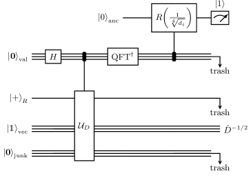
Figure 3: Quantum circuit for square-root degree matrix inversion. Note that QFT denotes quantum Fourier transform and $\mathcal{U}_{D}$ is defined by (18).

After the conditional rotation on the ancilla qubit “anc”, the state is

$$\sum_{i=0}^{N-1}\quantity(\sqrt{1-\sqrt{\frac{\check{C}}{d_{i}}}}\ket{0}_{\text{anc}}+\sqrt[4]{\frac{\check{C}}{d_{i}}}\ket{1}_{\text{anc}})\\ \otimes\ket{\widetilde{d_{i}}}_{\text{val}}\otimes\ket{+}_{R}\otimes\ket{i}_{\text{vec}}\otimes\ket{{\bf\it 0}}_{\text{junk}},$$ (20)

where $\check{C}$ is of order $O(d_{\text{min}})$. We then perform post-selection on the outcome “1” on the ancilla qubit and take the partial trace over “val”, “R”, and “junk” registers to obtain

$$\hat{D}^{-1/2}=\tilde{C}\sum_{i=0}^{N-1}\sqrt{\frac{1}{d_{i}}}\outerproduct{i}{i},$$ (21)

where $\tilde{C}=O\quantity(\quantity{\sum_{i=0}^{N-1}d_{i}^{-1/2}}^{-1})$ with success probability $\Omega\quantity(1/\kappa_{D}^{0.5})$ [28]. The success probability can be amplified to near certainty by repeating $O(\kappa_{D}^{0.25})$ rounds of amplitude amplification on the ancilla register [27]. Via another multiplication subroutine, we now have an access to the symmetrized transition matrix $S=D^{-1/2}KD^{-1/2}$ in an efficient manner.

Although we will not deal with the bona fide transition matrix $P$ in the rest of this work, it is important to note that $P=D^{-1}K=D^{-1/2}D^{-1/2}K$ can be efficiently constructed via the multiplication subroutine, given that we already have an access to $D^{-1/2}$ and $K$. In particular, the exponential $e^{iX_{3}(P)\tau}$ can be constructed in roughly $O(\kappa_{D}^{0.625}\tau^{1.5}\log^{2}N)$ steps (same as $T_{S}(\tau)$ in Theorem 1). Our algorithm thus can result in $P$ as a byproduct, which may be useful for other random-walk based algorithms.

V Eigen-decomposition

Recall that the necessary ingredients for constructing the diffusion map are the (right) eigenvectors and the eigenvalues of the transition matrix $P=D^{-1}K$. We thus need to solve the eigenvalue problem

$$D^{-1}K\ket{v_{i}}=\lambda_{i}\ket{v_{i}}.$$ (22)

Quantum phase estimation (QPE) would immediately provide such an eigen-decomposition if $P$ is symmetric, which is typically not the case. Note that if one applies QPE to the hermitized $\matrixquantity(0&P\\ P^{\dagger}&0)$, one would end up with the singular vectors of $P$, rather than the desired eigenvectors of nonsymmetric $P$. Therefore, we are in fact dealing with the generalized or nonsymmetric eigenvalue problem.

One resolution is to transform (22) to a standard symmetric eigenvalue problem

$$D^{-1/2}KD^{-1/2}\ket{s_{i}}=\lambda_{i}\ket{s_{i}},$$ (23)

where $\ket{s_{i}}\equiv D^{1/2}\ket{v_{i}}$. Then, the desired eigenvectors $\ket{v_{i}}$ can be recovered given an efficient rotation conditional on $D^{-1/2}.$ Now QPE can be applied, the output of which will be an estimate of the eigenvalues and the eigenvectors of

$$X_{3}(S)=(R_{3}+R_{3}^{\dagger})\otimes S$$ (24)

which are $\{\pm\lambda_{i}\}_{i=0}^{N-1}$ and $\ket{\pm}\otimes\ket{s_{i}}$. The rest of this section elaborates on the procedure for an eigen-decomposition of $S$, and on how to extract the eigenpairs of $P$ in order to construct the diffusion map classically.

V.1 Transition matrix eigen-decomposition

The complete quantum circuit for the eigen-decomposition of $P$ is shown in Fig. 4. An input state is prepared in registers “val”, “R” and “vec” as

$$\ket{{\bf\it 0}}_{\text{val}}\otimes\ket{+}_{R}\otimes\ket{\psi_{0}}_{\text{vec}}=\ket{{\bf\it 0}}_{\text{val}}\otimes\ket{+}_{R}\otimes\sum_{i=0}^{N-1}\beta_{i}\ket{s_{i}}_{\text{vec}},$$ (25)

where $\ket{\psi_{0}}$ is an arbitrary initial state such that $\beta_{i}\equiv\innerproduct{s_{i}}{\psi_{0}}$. The output state of the QPE after evolving for time $t=2\pi/\epsilon_{S}$, where $\epsilon_{S}$ is the accuracy of the estimated phases, reads

$$\ket{\psi_{1}}_{\text{val},R,\text{vec}}\equiv\sum_{i=0}^{N-1}\beta_{i}\ket{\widetilde{\lambda_{i}}}_{\text{val}}\otimes\ket{+}_{R}\otimes\ket{s_{i}}_{\text{vec}},$$ (26)

where $\widetilde{\lambda_{i}}$ denotes the binary representation of the estimated eigenvalues in the range $[0,1)$.

The resulting eigenvectors $\ket{s_{i}}$ are not yet the components of the diffusion map; they need to be conditionally rotated to the right eigenvectors $\ket{v_{i}}=D^{-1/2}\ket{s_{i}}$ of $P$ via another QPE using $e^{iX_{3}(D)t}$ as the time evolution operator. (Note that this step is more similar to the original HHL algorithm than our first application of QPE to construct $D^{-1/2}$. cf. [28]) For this reason, we add to the initial state register “deg” which will store the estimated eigenvalues $\widetilde{d_{i}}$ of the degree matrix, and register “junk” to eliminate the unwanted terms in (18):

$$\ket{\mathbf{0}}_{\text{deg}}\otimes\ket{\psi_{1}}_{\text{val},R,\text{vec}}\otimes\ket{\mathbf{0}}_{\text{junk}}.$$ (27)

The output of the QPE after evolving for time $t=O(\kappa_{D}^{0.5}/\epsilon_{D})$ is

$$\sum_{ij=0}^{N-1}\ket{\tilde{d_{j}}}_{\text{deg}}\otimes\beta_{i}\ket{\widetilde{\lambda_{i}}}_{\text{val}}\otimes\ket{+}_{R}\otimes(s_{i})_{j}\ket{j}_{\text{vec}}\otimes\ket{\mathbf{0}}_{\text{junk}},$$ (28)

where $(s_{i})_{j}$ is the $j^{\text{th}}$-component of $\ket{s_{i}}$. After the rotation conditioning on $\widetilde{d_{i}}$, and $O(\kappa_{D}^{0.5})$ rounds of amplitude amplification on an ancilla qubit as in (20) (not shown here), the eigenvector register is now, up to normalization, in the desired eigenstate

$$\sum_{j=0}^{N-1}\frac{(s_{i})_{j}}{\sqrt{d_{j}}}\ket{j}_{\text{vec}}=D^{-1/2}\ket{s_{i}}_{\text{vec}}=\ket{v_{i}}_{\text{vec}}.$$ (29)

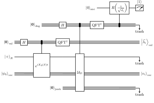
Figure 4: Quantum circuit for transition matrix $P$ eigen-decomposition. $\mathcal{U}_{D}$ is defined by (18).

V.2 Extracting desired eigenvalues and eigenvectors

Measuring the eigenvalue register “val” gives one of the eigenvalues and collapses the register “vec” to the eigenvector corresponding to that eigenvalue with probability $|\beta_{i}|^{2}$ (assuming no degeneracy as in the classical case (Sec. II.1)). The eigenvector can then be extracted using a number of copies that scales almost linearly in $N$ [33]. Repeating the procedure until we recover all $N-1$ distinct eigenvalues and eigenvectors allows us to classically construct the diffusion map (5).

The process of recovering all eigenpairs is not deterministic; in particular, one would not be able to recover an eigenpair for which $\beta_{i}$ is close to zero. What this means in practice is that one may need to change the initialization $\ket{\psi_{0}}$ of the QPE every so often, perhaps adaptively. We give below the expected runtime of this process in terms of the $\beta_{i}$’s of a fixed fiducial state based on the classical coupon collector’s problem [34]. Interestingly, in the best case where the $\beta_{i}$’s are all equal, the quantum coupon collector algorithm in [35] guarantees that we will see all eigenpairs at least once in time $O(N)$.

Input : Classical data $X$

Output : Eigenvalues $\{\lambda_{i}\}$ and right eigenvectors $\{{v}_{i}\}$ of the Markov transition matrix $P$

1. Embed $X$ into coherent state qRAM

2. Perform partial trace to obtain $\hat{K}$

3. Create state ${\hat{\mathbbm{1}}}$ and construct $e^{iX_{1}(\hat{K})t}$ and $e^{iX_{2}({\hat{\mathbbm{1}}})t}$

4. Construct $e^{iX_{3}(D)t}$ where $t=O\quantity(\kappa_{D}^{0.25}/\epsilon_{D})$

5. Invert square-root of $D$ by

   1. Using $e^{iX_{3}(D)t}$ in QPE initialized using state (19)

   2. Rotating the ancilla qubit controlled by the eigenvalue register “val”

   3. Amplifying an ancilla qubit “1” and perform partial trace on the “val”, “R”, and “junk” registers to get $\hat{D}^{-1/2}$

6. Construct $e^{iX_{3}(\hat{D}^{-1/2})t}$ and $e^{iX_{3}(S)t}$ where $t=O(1/\epsilon_{S})$

7. Use $e^{iX_{3}(S)t}$ in QPE initialized using state (25)

8. Operate $D^{-1/2}$ to obtain the eigen-decomposition of $P$ (29)

9. Measure the eigenvalue register “val” to get an approximated eigenvalue $\lambda_{i}$

10. Perform tomography to extract the eigenvector $v_{i}$ corresponding to the $\lambda_{i}$ measured in 9

Algorithm 1 Quantum diffusion map

VI Time Complexity of quantum diffusion map

The complexity of qDM is summarized in Theorem 1 and Lemma 1, the proof of which is provided in Appendix B. In Theorem 1, we provide the time complexity for performing eigen-decomposition of the transition matrix as we proposed in Sec. III - V. In Lemma 1, we provide the expected time complexity for reading out all eigenpairs using the classical coupon collector algorithm.

Theorem 1

(Time complexity of transition matrix eigen-decomposition) For a dataset $X=\{{\bf\it x}^{(i)}\}_{i=0}^{N-1}$ such that each ${\bf\it x}^{(i)}\in\mathbb{R}^{d}$ and $d<N$, steps 1-8 of Algorithm 1 constructs and eigen-decomposes the transition matrix with a runtime $T_{E}$ of

$$O\quantity(T_{S}\quantity(\frac{1}{\epsilon_{S}})\cdot\frac{\log N}{\epsilon_{S}}+T_{D}\quantity(\frac{\kappa_{D}^{0.5}}{\epsilon_{D}})\cdot\frac{\kappa_{D}^{0.5}\log N}{\epsilon_{D}}),$$ (30)

where $T_{D}$ denotes the time complexity to construct the degree matrix

$$T_{D}(t)=O\quantity(\quantity(\frac{t^{1.5}}{\epsilon_{m}^{0.5}}+\frac{t^{1.25}}{\epsilon_{e}\epsilon_{m}^{0.75}})\log N),$$ (31)

$T_{S}$ denotes the time complexity to construct the symmetrized transition matrix,

$$O\left(\quantity(\frac{\kappa_{D}^{0.625}}{\epsilon_{D}^{2.5}\epsilon_{m}^{0.5}}+\frac{\kappa_{D}^{0.5625}}{\epsilon_{D}^{2.25}\epsilon_{e}\epsilon_{m}^{0.75}})\quantity(\frac{t^{1.5}}{\epsilon_{m}^{0.5}\epsilon_{e}}+\frac{t}{\epsilon_{e}})\log^{2}N+\frac{t^{1.5}}{\epsilon_{m}^{0.5}\epsilon_{e}}\log N\right),$$ (32)

and $\epsilon_{e}$ and $\epsilon_{m}$ denote the errors of density matrix exponentiation and matrix multiplication, respectively.

Expressing equation (30), we simplify the time complexity of the transition matrix eigen-decomposition to

$$O\quantity(\kappa_{D}^{0.625}\log^{3}{N}+\kappa_{D}^{1.25}\log^{2}{N}).$$ (33)

Lemma 1

The expected runtime to construct the diffusion map given a fixed initialization (25) of the QPE is upper bounded by

$$\frac{\max_{i}\quantity{|\beta_{i}|^{2}}}{\min_{i}\quantity{|\beta_{i}|^{2}}}N\log N\cdot O\quantity(\frac{N}{\epsilon_{t}}\log N)\cdot T_{E}$$ (34)

where $i\in\{0,\cdots,N-1\}$, $T_{E}$ denotes the time complexity of eigen-decomposing the transition matrix in Theorem 1 and $\epsilon_{t}$ denotes the error of quantum tomography.

In the special case when all the $\beta_{i}$’s are equal, we can recover the worst-case runtime by virtue of the recent quantum coupon collector algorithm [35].

Lemma 2

Suppose that the QPE is initialized in the state such that all the $\beta$’s are equal in (25). Using the notations of Lemma 1, Algorithm 1 constructs the quantum diffusion map with a total runtime of

$$O\quantity(\frac{N^{2}}{\epsilon_{t}}\log N\cdot T_{E}).$$ (35)

When the errors and the condition number are independent of the dataset size $N$, the expected runtime reduces to

$$N^{2}\text{polylog}\,N,$$ (36)

compared to the classical diffusion map algorithm which requires $O(N^{3})$ time in the worst case. In fact, the bottleneck factor of $N^{2}$ and the probabilistic nature of the runtime solely arises from the readout (tomography) alone (see Appendix B), which perhaps can be circumvented if one coherently outputs the diffusion map as quantum states, providing an end-to-end computation. Another possibility to bypass the probabilistic runtime is to extend the quantum coupon collector algorithm in Lemma 2 to encompass a structured $\beta_{i}$’s and derive the worst case runtime. However, we leave this open problem for future work. Regarding the condition number of the degree matrix, the condition number $\kappa_{D}$ depends on the neighborhood connectivity of the dataset, which shall be tuned to be $O(1)$ and independent of $N$, provided the scale of the neighborhood controlled by $\sigma$ in the Kernel matrix is local, such as in Fig. 1 (middle).

VII Discussion and conclusion

In this work, we first review classical diffusion map, an unsupervised learning algorithm for nonlinear dimensionality reduction and manifold learning. We then explain our efforts to construct quantum algorithm for diffusion map. Our quantum diffusion map (qDM) consists of 5 major steps: coherent state data encoding scheme, a natural construction of kernel matrix from coherent states, a scheme to construct the Markov transition matrix from the kernel matrix, the eigen-decomposition of the transition matrix, and extracting relevant quantum information to construct diffusion map classically. The expected time complexity of qDM is $N^{2}\text{polylog}\,N$, compared to the worst-case runtime $O(N^{3})$ of a classical DM. Importantly, from accessing of qRAM to performing an eigen-decomposition of the Markov transition matrix, the total time complexity is only $O(\log^{3}N)$. Such exponential speedup for transition matrix construction and analysis could be useful in random walk-based algorithms.

Note that other recently proposed quantum algorithms for manifold learning include quantum kernel principal component analysis (qKPCA) [19] and quantum spectral clustering [21]. However, qDM has an appealing distance-preserving embedding property (6), neither possessed by qKPCA nor quantum spectral clustering. The inner working of qDM is also starkly different from those of qKPCA and quantum spectral clustering. While qKPCA relies on approximating an arbitrary target kernel via the truncated Taylor’s expansion of linear kernels [19], qDM proposes a method to exactly encode a Gaussian kernel from classical data, provided accessibility to qRAM. In addition, although both qDM and quantum spectral clustering are based on spectral graph methods, qDM manages to explicitly and efficiently construct the degree matrix inverse and the Markov transition operator, whose construction was mentioned not to be accessible efficiently [21]. Therefore, our work could provide a hint to achieve a quantum speedup in other algorithms that require a Markov transition operator and the analysis of its spectral properties.

Regarding the $N^{2}$ bottleneck, a quantum algorithm for the generalized coupon collector’s problem to speedup the process of finding all eigenpairs or a method to sort the eigenvalues and select only the top ones would reduce the complexity. Alternatively, one could devise a qDM algorithm that outputs the eigenvectors as quantum states and retain the exponential speedup. We leave open the question of how one could make use of such state for nonlinear dimensionality reduction.

Recently, manipulation of matrices and their spectra by block-encoding into submatrices of unitary matrices has become a topic of great interest due to its versatility in quantum algorithm design [36, 37], which may provide an alternative route to qDM algorithm.

Appendix A QMAT matrix multiplication subroutine

As explained in Sec. IV.1, all QMAT subroutines [26] utilized in our work reduce to that of matrix multiplication, which we now describe. Given matrices $A_{1}$ and $A_{2}$, the idea of the multiplication subroutine is to construct a Hermitian embedding of the product $A_{1}A_{2}$,

$$X_{3}(A_{1}A_{2})=\matrixquantity(0&0&A_{1}A_{2}\\ 0&0&0\\ (A_{1}A_{2})^{\dagger}&0&0),$$

from the following commutator:

$$X_{3}(A_{1}A_{2})=UX_{3}(iA_{1}A_{2})U^{\dagger}=iU[X_{1}(A_{1}),X_{2}(A_{2})]U^{\dagger},$$ (37)

where

$$U=\matrixquantity(\sqrt{-i}I&0&0\\ 0&I&0\\ 0&0&\sqrt{i}I).$$

Thus, the goal is to simulate the commutator of two hermitian operators. This can be accomplished with bounded error via the second order of the Baker-Campbell-Hausdorff formula. Define

$$\tilde{l}(x,y)\equiv e^{x}e^{y}e^{-x}e^{-y}e^{-x}e^{-y}e^{x}e^{y}.$$

With the step size $t/m$, we have that [26],

$$\tilde{l}(xt/m,yt/m)=e^{2[x,y]t^{2}/m^{2}+O(t^{4}/m^{4})}.$$ (38)

Thus, iterating the above $n^{\prime}=m^{2}/(2t)=O(t^{2}/\epsilon_{m})$ times,

$$\tilde{l}\left(xt/m,yt/m\right)^{n^{2}/(2t)}=e^{[x,y]t+O(t^{3}/m^{2})},$$ (39)

correctly simulates $e^{[x,y]t}$ up to an error $\epsilon_{m}=O(t^{3}/m^{2})$.

Putting all these together, the QMAT multiplication subroutine consumes $n^{\prime}=m^{2}/(2t)$ copies of $e^{iX_{1}(A_{1})t/m}$ and $e^{iX_{2}(A_{2})t/m}$ (and their inverses), and outputs a unitary operator

$$U[l(iX_{1}(A_{1})t/m,iX_{2}(A_{2})t/m)]^{n^{\prime}}U^{\dagger},$$ (40)

that approximates $e^{iX_{3}(A_{1}A_{2})}$ up to an error $\epsilon_{m}$ in the operator norm.

Appendix B Complexity analysis

This section describes the calculation for the time complexity that leads to the result in Theorem 1. We separate the algorithm into sequential steps as we have done with the classical DM (Sec. II.2), namely, the embedding of classical data into the kernel $\hat{K}$, the calculation of the transition matrix $P$, and the calculation of the eigen-decomposition.

B.1 Preparing the kernel

In creating $\hat{K}$, we consider only the time complexity coming from storing classical data into qRAM (Sec. III.1) as partial trace does not create additional time cost. Here we have assumed a common position among researchers in the field that encoding of classical data can be made efficient via the existence of an oracle [18, 38, 28, 22, 39, 31], and analyze the algorithm based on this assumption. Note that practical feasibility and resource estimate of implementing qRAM is still an ongoing research topic [31, 40, 41, 42, 43]. Assuming that the data consists of $N$ vectors each with $d$ features, the data can be encoded into a qRAM of the size $dN$, which can be accessed using $O(\log(dN))$ operations (11) [38]. We assume here that we are dealing with big data, i.e., $d\leq N$. Therefore, the time cost becomes $O(\log N^{2})=O(\log N)$.

B.2 Calculating the transition matrix

Next, we construct the exponential of $P$. We start with exponentiating the necessary matrices. Then we multiply these matrices in order to create $\text{e}^{\imath X_{3}(D)t}$. Next, we inverse the degree matrix $D$ before constructing the transition matrix $P=D^{-1}K$.

The time cost of creating exponentials depends on whether the quantum simulation of matrices or quantum state is used. Creating exponentials from multiple copies of density matrices, i.e., $e^{iX_{3}(\hat{K})t}$ and $e^{iX_{3}(\hat{{\mathbbm{1}}})t}$ , results in a time complexity of $O(t^{2}/\epsilon_{e})$, where $\epsilon_{e}$ is the accuracy for the exponentiation [18]. Combined with the number of operations for storing the states, which is $O(\log N)$, the time complexity is $O(t^{2}/\epsilon_{e}\log N)$.

Exponentials of sparse matrices can be simulated using the method in [29] with query complexity of $O\quantity(t+\frac{\log(1/\epsilon_{s})}{\log\log(1/\epsilon_{s})})$, where $\epsilon_{s}$ is the accuracy of the method. For the matrices $e^{iX_{3}(\Xi)t}$ and $e^{iX_{3}(\Xi^{\dagger})t}$, we also need to take into account the gate complexity $O(\log N)$. Thus the time complexity for preparing each of these exponentials is $O(t\log N)$.

To construct the degree matrix, we use the matrix multiplication subroutine in Appendix A. This subroutine uses 4 copies of each input exponential, which is multiplied and then applied $n^{\prime}$ times. In creating $e^{iX_{3}(\hat{K}{\mathbbm{1}}\otimes I)}$ (Sec. IV.1), the time cost comes from multiplying the exponential of $\hat{K}$ and of ${\mathbbm{1}}$ whereas $\otimes I$ is assumed to be a free operation. Therefore, the time cost is $O\quantity(n^{\prime}\quantity(\frac{t^{2}}{m^{2}\epsilon_{e}}\log N))$. Given the condition that $n^{\prime}=\frac{m^{2}}{2t}=O\left(\frac{t^{2}}{\epsilon_{m}}\right)~{}$[26], we rewrite the time cost to $O(t\log N\epsilon_{e}^{-1})$.

In the next two steps, we multiply $\Xi$ and $\Xi^{\dagger}$ into $K{\mathbbm{1}}\otimes I$. Again, we apply the multiplication subroutine iteratively with 4 copies of the result from the previous multiplication as one of the input. These steps admit additional order of $\epsilon_{m}$ and $t$ which leads the time cost of $e^{iX_{3}(D)t}$ to be

$$T_{D}(t)=O\quantity(\quantity(\frac{t^{1.5}}{\epsilon_{m}^{0.5}}+\frac{t^{1.25}}{\epsilon_{e}\epsilon_{m}^{0.75}})\log N).$$ (41)

Next, the degree matrix $D$ is inverted (Sec. IV.2) by first performing QPE that takes the prepared $e^{iX_{3}(D)t}$ as the unitary operator in QPE then a controlled rotation. The time cost of the QPE is $O(T_{D}/\epsilon_{D}\log m)$ [44], where $m$ is the number of eigenvalues which is $m=N$, and $\epsilon_{D}$ is the error of estimated phase. Assuming the controlled rotation is executed in time $O(1)$, we have accumulated a time cost of $T_{D}+O(T_{D}/\epsilon_{D}\log N)+O(1)$. The time complexity is thus dominated by $O(T_{D}/\epsilon_{D}\log N)$.

The time $T_{D}$ (41) is a function of $t$, which we now find through error analysis of matrix inversion. As we are inverting the eigenvalues of $D$ to a function of $1/\sqrt[4]{x}$ [28], the error after conditional rotation becomes $\epsilon_{D}=O(1/\sqrt[4]{d_{i}}t)<O(\kappa_{D}^{0.25}/t)$. Thus $t=O(\kappa_{D}^{0.25}/\epsilon_{D})$.

As the success probability of measuring $\ket{1}$ in the ancilla qubit is $\Omega(1/\kappa_{D}^{0.5})$, the number of rounds necessary to obtain a successful result is $O(\kappa_{D}^{0.5})$. To accelerate the process, we use the amplitude amplification to amplify the success probability in $O(\kappa_{D}^{0.25})$ steps. Thus an overall complexity becomes

$$T_{D^{-1/2}}=O\quantity(\quantity(\frac{\kappa_{D}^{0.625}}{\epsilon_{D}^{2.5}\epsilon_{m}^{0.5}}+\frac{\kappa_{D}^{0.5625}}{\epsilon_{D}^{2.25}\epsilon_{e}\epsilon_{m}^{0.75}})\log^{2}N).$$ (42)

The last step in constructing the symmetrized transition matrix is multiplying inverse square-root degree matrix to $\hat{K}$, which we perform in the exponential (Sec. IV.2). Therefore, we first need to exponentiate $D^{-1/2}$ and $\hat{K}$ using a time of $O(t^{2}/(m^{2}\epsilon_{e}))$ and $4n^{\prime}$ copies each. The time complexity for constructing $e^{iX_{3}(S)t}$ is therefore

$$T_{S}(t)=O\quantity(T_{D^{-1/2}}\cdot\quantity(\frac{t^{1.5}}{\epsilon_{m}^{0.5}\epsilon_{e}}+\frac{t}{\epsilon_{e}})+\frac{t^{1.5}}{\epsilon_{m}^{0.5}\epsilon_{e}}\log N).$$

B.3 Eigen-decomposition

In this subsection, we find the eigenvalues and eigenvectors of $S$, using a second QPE algorithm (Sec. V). We take $t=O(1/\epsilon_{S})$ to perform the QPE in time $O(\log N)$ with accuracy $\epsilon_{S}$ [44].

The third and final QPE is required to transform $\ket{s_{i}}$ to the right eigenvector $\ket{v_{i}}=D^{-1/2}\ket{s_{i}}$ of the transition matrix $P=D^{-1}K$. The complexity analysis proceeds analogously to the analysis in Sec B.2: the error analysis of matrix inversion gives $t=O(\kappa_{D}^{0.5}/\epsilon_{D})$. As the success probability of measuring $\ket{1}$ in the ancilla qubit is $\Omega(1/\kappa_{D})$, the number of rounds necessary to obtain a successful result is $O(\kappa_{D})$. To accelerate the process, amplitude amplification is used to amplify the success probability in $O(\kappa_{D}^{0.5})$ steps. Incorporating the time required to prepare copies of $e^{iX_{3}(D)t}$, the time complexity of the conditional rotation is hence $O(T_{D}(\kappa_{D}^{0.5}/\epsilon_{D})\cdot\kappa_{D}^{0.5}\log N/\epsilon_{D})$. Thus, the overall complexity of the eigen-decomposition of the transition matrix becomes

$$O\quantity(T_{S}\quantity(\frac{1}{\epsilon_{S}})\cdot\frac{\log N}{\epsilon_{S}}+T_{D}\quantity(\frac{\kappa_{D}^{0.5}}{\epsilon_{D}})\cdot\frac{\kappa_{D}^{0.5}\log N}{\epsilon_{D}}),$$ (43)

which proves Theorem 1.

We repeat the QPE and measure the eigenvalue register in the computation basis until we find sufficiently many copies of all eigenpairs for tomography. The process is not deterministic and we can only talk about the expected number of repetitions required. The task of drawing items (with replacement) distributed according to a given probability distribution $\{p_{i}\}_{i=1}^{N}$ until one collects all $N$ distinct items is known as the coupon collector’s problem, and an upper bound on the expected number of draws is known to be $(\max_{i}\{p_{i}\}/\min_{i}\{p_{i}\})N\log N$ [34]. Once we repeat the QPE and measure the eigenvalue register in the computation basis until we obtain $O(N\log N/\epsilon_{t})$ copies of each eigenpair, the pure-state tomography algorithm of [33] recovers a classical vector that is $\epsilon_{t}$-close in $\ell_{2}$-norm to the eigenvector. The above facts together with Theorem 1 immediately implies Lemma 1.

Finally, in the case of uniformly random coupons i.e. $p_{i}=p_{j}$ for all $i,j\in\{1,\dots,N\}$, there exists a gate-efficient quantum algorithm that solves the coupon collector problem in time $O(N)$ [35], giving Lemma 2.