RAPTOR: End-to-end Risk-Aware MDP Planning and Policy Learning by Backpropagation

Abstract

Planning provides a framework for optimizing sequential decisions in complex environments. Recent advances in efficient planning in deterministic or stochastic high-dimensional domains with continuous action spaces leverage backpropagation through a model of the environment to directly optimize actions. However, existing methods typically not take risk into account when optimizing in stochastic domains, which can be incorporated efficiently in MDPs by optimizing the entropic utility of returns. We bridge this gap by introducing Risk-Aware Planning using PyTorch (RAPTOR), a novel framework for risk-sensitive planning through end-to-end optimization of the entropic utility objective. A key technical difficulty of our approach lies in that direct optimization of the entropic utility by backpropagation is impossible due to the presence of environment stochasticity. The novelty of RAPTOR lies in the reparameterization of the state distribution, which makes it possible to apply stochastic backpropagatation through sufficient statistics of the entropic utility computed from forward-sampled trajectories. The direct optimization of this empirical objective in an end-to-end manner is called the risk-averse straight-line plan, which commits to a sequence of actions in advance and can be sub-optimal in highly stochastic domains. We address this shortcoming by optimizing for risk-aware Deep Reactive Policies (RaDRP) in our framework. We evaluate and compare these two forms of RAPTOR on three highly stochastic domains, including nonlinear navigation, HVAC control, and linear reservoir control, demonstrating the ability to manage risk in complex MDPs.

1 Introduction

As machine learning models are more frequently deployed in the real world, the concern over ensuring their safety has been ever-increasing [9, 23]. In sequential stochastic decision-making problems, it has been shown that optimizing the expected cumulative reward can lead to undesirable outcomes such as excessive risk-taking, since low-probability catastrophic outcomes with negative reward, or risk, can be underrepresented [20]. The risk-averse MDP framework addresses this problem by optimizing risk measures with favorable mathematical properties [27].

On the other hand, planning optimizes decisions or actions given a mathematical description of the environment, thus minimizing the need to do dangerous exploration in the real world. However, despite advances in scalable end-to-end planning, existing approaches do not typically take risk into account. For instance, BackpropPlan [30] utilizes recent advances in deep learning and is highly scalable in continuous state or action spaces (CSA-MDPs). In this framework, the transition model and reward are encoded in RNN-like cells. Unlike a typical neural network, the inputs to the network are the actions that are optimized through backpropagation. By employing highly effective tools for non-convex optimization [29], BackpropPlan is able to efficiently learn optimal sequences of actions. However, its main limitation is that it cannot be applied to stochastic models, which could be addressed by learning reactive policies [4]. However, neither approach incorporates risk explicitly.

One popular approach for incorporating risk-sensitivity into MDPs is the entropic utility, as well as its mean-variance approximation, which can be interpreted as trade-offs between the mean and the variance of the cumulative return [1]. One key advantage of the entropic utility is that it is defined entirely in terms of expectation operators, rather than percentiles or other quantities that can more difficult to estimate from sample trajectories, making it an intuitive starting point for scalable planning. Furthermore, the entropic utility satisfies a recursive property [21] that makes it possible to optimize directly in sequential decision-making problems without relying explicitly on the Bellman principle, which often presents computational challenges in other risk-aware MDP and reinforcement learning frameworks [7, 18]. This makes it particularly suitable for gradient-based end-to-end planning.

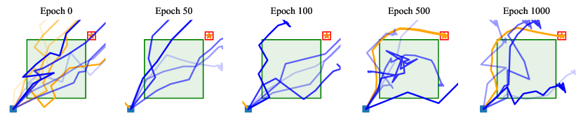
Figure 1: The evolution of trajectories navigated by RAPTOR (orange) and a risk-neutral agent (blue) in a two-dimensional Navigation domain subject to stochastic dynamics (note: multiple sample trajectories are shown simultaneously in each epoch). The green bounding box at the center is a high-variance zone. The more an agent traverses into the box the higher the variability in the next position at which the agent lands. The blue square on the bottom left is the starting position, while the red box at the upper right corner shows the goal region. By epoch $1000$, we clearly see that the risk-sensitive agent is able to get to the goal region by avoiding the box and thus failure, while the risk-neutral agent does not.

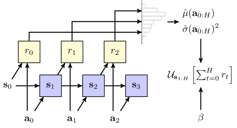
Figure 2: A simplified decision diagram for planning with an entropic utility objective of the return, $\mathcal{U}\!\left(\sum_{t}r_{t}\right)$. Here, the sufficient statistics of the return distribution, namely mean $\hat{\mu}$ and variance $\hat{\sigma}^{2}$ are computed by forward sampling state trajectories and used to approximate the utility. Applying the reparameterization trick and backpropagation will lead to our overall approach RAPTOR.

To this end, we propose RAPTOR (Risk-Aware Planning using pyTORch), which enables scalable risk-aware end-to-end planning for CSA-MDPs by leveraging automatic differentiation [22] for gradient-based optimization w.r.t. the MDP model and an entropic utility objective. To achieve this, we begin by leveraging an extension of BackpropPlan to accommodate stochastic transitions [4], by representing the planning domain as a stochastic computation graph (Section 3.1). While we cannot directly formalize the distributionally-defined entropic utility in closed-form for end-to-end planning, for many classes of problems we can reparameterize the objective and apply stochastic backpropagation. This allows us to compute the entropic utility directly from the sufficient statistics of forward-sampled trajectories, while still permitting backpropagation through the utility and its symbolic computation from sufficient statistics of trajectories. We then leverage these computational results to propose two approaches for optimizing risk-aware decisions (Section 3.2). The first derives a risk-sensitive straight-line plan, in which the agent commits to a sequence of actions in advance, while the second learns a deep reactive policy and is particularly suited for highly stochastic domains. Both approaches integrate seamlessly into our optimization framework, and can be computed efficiently in an end-to-end manner by reparameterization and backpropagation.

Indeed, as evidenced by Figure 1, RAPTOR is effective at finding risk-averse behaviors in highly stochastic environments in a computationally efficient manner. Overall, empirical evaluations in Section 4 on three highly stochastic domains involving continuous action parameters — navigation, HVAC control, and reservoir control — demonstrate that RAPTOR is a reliable and efficient end-to-end method for risk-sensitive planning in complex MDPs.

2 Preliminaries

2.1 Continuous State-Action Markov Decision Process (CSA-MDP)

Sequential decision-making problems in this work are modeled as continuous state-action Markov decision processes (CSA-MDPs), defined as tuples $\langle\mathcal{S},\mathcal{A},r,p,\mathbf{s}_{0}\rangle$: $\mathcal{S}\subseteq\mathbb{R}^{n}$ is the state space, $\mathcal{A}\subseteq\mathbb{R}^{m}$ is the action space, $r:\mathcal{S}\times\mathcal{A}\to\mathbb{R}$ is a bounded differentiable reward function, $p:\mathcal{S}\times\mathcal{A}\times\mathcal{S}\to[0,\infty)$ describes the non-linear dynamics of the system, and $\mathbf{s}_{0}$ is the initial state. Note that CSA-MDPs are naturally factored [3], such that the state components are mutually independent given the previous state $\mathbf{s}_{t}$ and action $\mathbf{a}_{t}$.

In the risk-neutral setting, the objective function to optimize is the expected return,

$$V_{h}(\mathbf{a}_{h:H})\vcentcolon=\mathbb{E}_{\mathbf{s}_{h+1:H}}\!\left[\sum_{t=h}^{H}r(\mathbf{s}_{t},\mathbf{a}_{t})\right],$$ (1)

where state trajectories $\mathbf{s}_{h+1:H}=\mathbf{s}_{h+1},\mathbf{s}_{h+2},\dots\mathbf{s}_{H}$ are sampled according to $p$ and actions can either be computed from a closed-loop reactive policy $\pi$, e.g. $\mathbf{a}_{t}=\pi_{t}(\mathbf{s}_{t})$, or an open-loop policy or plan $\mathbf{a}_{h:H}=\mathbf{a}_{h},\mathbf{a}_{h+1},\dots\mathbf{a}_{H}$.

2.2 Risk-Aversion in CSA-MDPs

Risk sensitivity can be incorporated into the agent’s decision-making by replacing the expectation operator $\mathbb{E}_{\mathbf{s}_{h+1:H}}\!\left[\cdot\right]$ with a non-linear utility function. In this paper, we consider the entropic utility, that for $\beta\in\mathbb{R}$ and a random variable $X$ is defined as

$$\mathcal{U}\!\left(X\right)\vcentcolon=\frac{1}{\beta}\log\mathbb{E}\!\left[e^{\beta X}\right].$$ (2)

Taylor expansion of (2) obtains the mean-variance approximation

$$\mathcal{U}\!\left(X\right)=\mathbb{E}\!\left[X\right]+\frac{\beta}{2}\mathrm{Var}\!\left[X\right]+O(\beta^{2}).$$ (3)

Now, interpreting variance as risk, $\beta$ can be interpreted as the overall level of risk aversion of the agent: $\beta=0$ induces risk-neutral behavior, while choosing $\beta>0$ ($\beta<0$) induces risk-seeking (risk-averse) behaviors. Thus for a risk-averse agent, the entropic utility can provide protection against high return variability. In addition, the entropic utility is perhaps the most well-known convex/concave utility, which means it is monotone, translation invariant, and concave for $\beta<0$, properties that are often seen as minimal requirements for developing rational decision-making [12, 17].

Generalizing (1) to the risk-aware setting, we define the utility of an action sequence as

$$U_{h}(\mathbf{a}_{h:H})\vcentcolon=\mathcal{U}_{\mathbf{s}_{h+1:H}}\!\left(\sum_{t=h}^{H}r(\mathbf{s}_{t},\mathbf{a}_{t})\right),$$ (4)

where it is understood that expectations are computed w.r.t. the distribution of $\mathbf{s}_{h+1:H}$. Furthermore, due to the recursive property of entropic utility [1, 8, 21], the optimal utility-to-go ${U}^{*}_{h}\!\left(\mathbf{s}_{h}\right)\vcentcolon=\sup_{\pi}\,U_{h}(\mathbf{a}_{h:H})$ over closed-loop policies satisfies the Bellman equation

$${U}^{*}_{h}\!\left(\mathbf{s}_{h}\right)=\sup_{\mathbf{a}_{h}\in\mathcal{A}}\,\mathcal{U}_{\mathbf{s}_{h+1}}\!\left(r(\mathbf{s}_{h},\mathbf{a}_{h})+{U}^{*}_{h+1}\!\left(\mathbf{s}_{h+1}\right)\right),$$ (5)

that is analogous to the risk-neutral setting [24]. Furthermore, the entropic utility is the only convex/concave utility that can be written in this way [16]. This makes the entropic utility particularly suitable for learning policies and planning in CSA-MDPs.

3 Risk-Aware Planning

The goal of planning is to avoid the expensive computation of (5). In this section, we formally define our proposed method, RAPTOR, that computes a policy or plan for the risk-sensitive objective (4) by optimizing it directly in an end-to-end manner. To this end, we employ stochastic computation graphs and the reparameterization trick for the entropic utility.

3.1 Risk-Aware End-to-End Planning by Backpropagation

We begin with the idea of learning optimal open-loop policies for the utility objective (4) using gradient descent:

$$\frac{\partial U_{h}(\mathbf{a}_{h:H})}{\partial\mathbf{a}_{t}} =\frac{\partial}{\partial\mathbf{a}_{t}}\left(\frac{1}{\beta}\log\mathbb{E}_{\mathbf{s}_{h+1:H}}\!\left[\exp{\left(\beta\sum_{t=h}^{H}r(\mathbf{s}_{t},\mathbf{a}_{t})\right)}\right]\right)$$

$$\propto\frac{\partial}{\partial\mathbf{a}_{t}}\mathbb{E}_{\mathbf{s}_{h+1:H}}\!\left[\exp{\left(\beta\sum_{t=h}^{H}r(\mathbf{s}_{t},\mathbf{a}_{t})\right)}\right],$$ (6)

where we have ignored the denominator for ease of exposition. However, backpropagating through the expectation (6) requires backpropagating through the entire sequence of state trajectories $\mathbf{s}_{h},\mathbf{s}_{h+1}\dots$, since $\mathbf{s}_{t+1}\sim p\!\left(\left.\kern-1.2pt\cdot\,\right|\,\mathbf{s}_{t},\mathbf{a}_{t}\right)$ depends implicitly on the actions. The difficulty therefore lies in our inability to directly backpropagate through the stochastic transitions that are not inherently differentiable.

Reparameterization Trick

Instead, we employ the widely-used reparameterization trick [2, 11, 15, 28], by rewriting a sample from the distribution $\mathbf{s}_{t+1}\sim p\!\left(\left.\kern-1.2pt\cdot\,\right|\,\mathbf{s}_{t},\mathbf{a}_{t}\right)$ as the output of a deterministic differentiable function $\phi:\mathcal{S}\times\mathcal{A}\times\Xi\to\mathcal{S}$:

$$\mathbf{s}_{t+1}=\phi(\mathbf{s}_{t},\mathbf{a}_{t},\xi_{t}),\quad\xi_{0},\xi_{1},\dots\xi_{H}\sim f_{\xi},\quad t=h,h+1,\dots H,$$ (7)

where $\xi_{0:H}=\xi_{0},\xi_{1},\dots\xi_{H}$ is a sequence of i.i.d. disturbances drawn from some distribution $f_{\xi}$ on $\Xi$, which we call a scenario. For practical illustration, if $p\!\left(\left.\kern-1.2pt\cdot\,\right|\,\mathbf{s}_{t},\mathbf{a}_{t}\right)$ belongs to a location-scale family, then $\phi(\mathbf{s}_{t},\mathbf{a}_{t},\xi_{t})=m(\mathbf{s}_{t},\mathbf{a}_{t})+\xi_{t}v(\mathbf{s}_{t},\mathbf{a}_{t})$ for some functions $m$ and $v$, and can be generalized to other distributions [26]. The reparameterization trick (7) now allows us to rewrite the state trajectory explicitly as a function of the initial state $\mathbf{s}_{h}$, previous actions and previous disturbances:

$$\mathbf{s}_{t} =\phi(\mathbf{s}_{t-1},\mathbf{a}_{t-1},\xi_{t-1})$$

$$=\phi(\phi(\mathbf{s}_{t-2},\mathbf{a}_{t-2},\xi_{t-2}),\mathbf{a}_{t-1},\xi_{t-1})$$

$$=\dots\vcentcolon=\Phi_{t}(\mathbf{s}_{h},\mathbf{a}_{h:t-1},\xi_{h:t-1}),\quad\forall t=h,h+1,\dots H.$$ (8)

Plugging (8) back into (6), the gradient can now be computed deterministically by sampling a scenario $\xi_{h:H}=\xi_{h},\xi_{h+1},\dots\xi_{H}$ a priori, and backpropagating through the expectation:

$$\frac{\partial U_{h}(\mathbf{a}_{h:H})}{\partial\mathbf{a}_{t}} \propto\frac{\partial}{\partial\mathbf{a}_{t}}\mathbb{E}_{\mathbf{s}_{h+1:H}}\!\left[\exp{\left(\beta\sum_{t=h}^{H}r(\mathbf{s}_{t},\mathbf{a}_{t})\right)}\right]$$

$$=\frac{\partial}{\partial\mathbf{a}_{t}}\mathbb{E}_{\xi_{h:H}}\!\left[\exp{\left(\beta\sum_{t=h}^{H}r(\Phi_{t}(\mathbf{s}_{h},\mathbf{a}_{h:t-1},\xi_{h:t-1}),\mathbf{a}_{t})\right)}\right]$$

$$=\mathbb{E}_{\xi_{h:H}}\!\left[\frac{\partial}{\partial\mathbf{a}_{t}}\exp{\left(\beta\sum_{t=h}^{H}r(\Phi_{t}(\mathbf{s}_{h},\mathbf{a}_{h:t-1},\xi_{h:t-1}),\mathbf{a}_{t})\right)}\right].$$

Planning Through Sufficient Statistics of the Return Distribution

While optimizing the exact entropic utility is possible, it can often overflow due to computing an exponential function of the return [13]. An alternative approach is to approximate the utility by the mean-variance approximation (3), in which the mean and variance of the return can be represented symbolically, and backpropagating through these sufficient statistics by again making use of the reparameterization trick (8):

$$U_{h}(\mathbf{a}_{h:H})=\mathcal{U}_{\mathbf{s}_{h+1:H}}\!\left(\sum_{t=h}^{H}r(\mathbf{s}_{t},\mathbf{a}_{t})\right)$$

$$\approx\mathbb{E}_{\mathbf{s}_{h+1:H}}\!\left[\sum_{t=h}^{H}r(\mathbf{s}_{t},\mathbf{a}_{t})\right]+\frac{\beta}{2}\mathrm{Var}_{\mathbf{s}_{h+1:H}}\!\left[\sum_{t=h}^{H}r(\mathbf{s}_{t},\mathbf{a}_{t})\right]$$

$$=\mathbb{E}_{\xi_{h+1:H}}\!\left[\sum_{t=h}^{H}r(\Phi_{t}(\mathbf{s}_{h},\mathbf{a}_{h:t-1},\xi_{h:t-1}),\mathbf{a}_{t})\right]+\frac{\beta}{2}\mathrm{Var}_{\xi_{h+1:H}}\!\left[\sum_{t=h}^{H}r(\Phi_{t}(\mathbf{s}_{h},\mathbf{a}_{h:t-1},\xi_{h:t-1}),\mathbf{a}_{t})\right].$$ (9)

Now (9) can be estimated via sample approximations, in which a finite number $m$ of scenarios $\xi_{h:H}^{i}\sim\prod_{t=h}^{H}f_{\xi}(\xi_{t})$ are forward-sampled to estimate $\mathbf{s}_{h}^{i},\mathbf{s}_{h+1}^{i},\dots\mathbf{s}_{H}^{i}$ and $r_{t}^{i}\vcentcolon=r(\mathbf{s}_{t}^{i},\mathbf{a}_{t})$:

$${U}_{h}(\mathbf{a}_{h:H}) \approx\hat{U}_{h}(\mathbf{a}_{h:H})\vcentcolon=\hat{\mu}_{h}(\mathbf{a}_{h:H})+\frac{\beta}{2}\hat{\sigma}_{h}(\mathbf{a}_{h:H})^{2}$$ (10)

$$\hat{\mu}_{h}(\mathbf{a}_{h:H}) \vcentcolon=\frac{1}{m}\sum_{i=1}^{m}\sum_{t=h}^{H}r_{t}^{i},\quad\hat{\sigma}_{h}(\mathbf{a}_{h:H})^{2}\vcentcolon=\frac{1}{m}\sum_{i=1}^{m}\left(\sum_{t=h}^{H}r_{t}^{i}-\hat{\mu}_{h}(\mathbf{a}_{h:H})\right)^{2}.$$

In other words, computing an optimal sequence of actions requires backpropagating through the sufficient statistics $\hat{\mu}_{h}(\mathbf{a}_{h:H})$ and $\hat{\sigma}_{h}(\mathbf{a}_{h:H})^{2}$ w.r.t. the action sequences $\mathbf{a}_{h:H}$. Through reparameterization, the gradients of the sample sufficient statistics (10) can now flow through $\phi$ end-to-end:

$$\frac{\partial\hat{U}_{h}(\mathbf{a}_{h:H})}{\partial\mathbf{a}_{t}} \approx\frac{\partial\hat{U}_{h}(\mathbf{a}_{h:H})}{\partial\mathbf{s}_{t+1}}\frac{\partial\mathbf{s}_{t+1}}{\partial\mathbf{a}_{t}}$$

$$=\frac{\partial\mathbf{s}_{t+1}}{\partial\mathbf{a}_{t}}\sum_{\tau=t+1}^{H}\frac{\partial\hat{U}_{h}(\mathbf{a}_{h:H})}{\partial r_{\tau}}\frac{\partial r_{\tau}}{\partial\mathbf{s}_{\tau}}\prod_{\kappa=\tau}^{t+2}\frac{\partial\mathbf{s}_{\kappa}}{\partial\mathbf{s}_{\kappa-1}}$$

$$=\frac{\partial\phi(\mathbf{s}_{t},\mathbf{a}_{t},\xi_{t})}{\partial\mathbf{a}_{t}}\sum_{\tau=t+1}^{H}\frac{\partial\hat{U}_{h}(\mathbf{a}_{h:H})}{\partial r_{\tau}}\frac{\partial r_{\tau}}{\partial\mathbf{s}_{\tau}}\prod_{\kappa=\tau}^{t+2}\frac{\partial\phi(\mathbf{s}_{\kappa-1},\mathbf{a}_{\kappa-1},\xi_{\kappa-1})}{\partial\mathbf{s}_{\kappa-1}},$$

where we have ignored the existence of multiple rollouts with index $i$ for ease of notation. In essence, actions that optimize the utility can now be computed by forward-sampling $\xi_{h:H}^{i}$, backpropagating through the utility’s sufficient statistics computed on the simulated scenarios $\xi_{h:H}^{i}$ and updating the actions by gradient descent, e.g. $\mathbf{a}_{t}^{\prime}=\mathbf{a}_{t}-\alpha\frac{\partial\hat{U}_{h}(\mathbf{a}_{h:H})}{\partial\mathbf{a}_{t}}$.

3.2 Risk-Aware Straight-Line Plan and Deep Reactive Policy

Risk-Aware Straight-Line Plan

The optimization of $\hat{U}_{h}(\mathbf{s}_{h})$ by backpropagation avoids the computationally expensive iteration of (5) while providing a maximizing plan $\mathbf{a}_{0:H}^{*}$. However, the plan computed above commits to a fixed sequence of actions starting from the initial state $\mathbf{s}_{0}$ and follows them until the end of the planning horizon. For this reason, we call this plan the risk-aware straight-line plan (SLP), and its corresponding utility

$$u_{SL}(\mathbf{s}_{0})\vcentcolon=\sup_{\mathbf{a}_{0:H}}\,\mathcal{U}_{\xi_{0:H}}\!\left(\sum_{t=0}^{H}r(\mathbf{s}_{t},\mathbf{a}_{t})\right).$$ (11)

The limitation of an SLP is that its utility could be lower than the closed loop policy in (5), since stochasticity prevents it from responding to significant deviations in states from their anticipated trajectory. On the other hand, (11) provides a (potentially tight) lower bound to the utility of the optimal closed-loop policy [19], and has been used extensively in risk-neutral planning [5, 14, 25]. We provide this lower bound in the risk-averse setting (see Appendix A.1) for a proof).

Theorem 1.

The quantity $u_{SL}(\mathbf{s}_{0})$ is a lower bound to the optimal utility, ${U}^{*}_{0}\!\left(\mathbf{s}_{0}\right)\geq u_{SL}(\mathbf{s}_{0})$.

Risk-Aware Deep Reactive Policy

In order to optimize CSA-MDPs without facing the potential limitations of computing straight-line plans, an alternative approach is to learn a risk-aware reactive policy, which is an explicit mapping from states to actions, e.g. $\pi_{t}:\mathcal{S}\to\mathcal{A}$ [4]. In order to realize efficient planning end-to-end, we can learn a parameterized policy $\pi_{\theta}$, where $\theta$ represent the weights of a parameteric model such as a neural network, in which case this reduces to a risk-aware instantiation of the deep reactive policy (DRP).

Reparameterization Trick for DRPs

The deep reactive policy depends on the state, which in turn depends implicitly on the previous action, which depends on the previous state, and so on, which makes the reparameterization of the entropic utility more involved. In this case, the reparameterization trick described in the previous section could be applied with respect to the DRP parameters:

$$\mathbf{s}_{t} =\phi(\mathbf{s}_{t-1},\pi_{\theta}(\mathbf{s}_{t-1}),\xi_{t-1})$$

$$=\phi(\phi(\mathbf{s}_{t-2},\pi_{\theta}(\mathbf{s}_{t-2}),\xi_{t-1}),\pi_{\theta}\left(\phi(\mathbf{s}_{t-2},\pi_{\theta}(\mathbf{s}_{t-2}),\xi_{t-1})\right),\xi_{t-1})$$

$$=\dots\vcentcolon=\Psi_{t}(\mathbf{s}_{h},\theta,\xi_{h:t-1}),\quad\forall t=h,h+1,\dots H.$$ (12)

Now, the DRP can be readily computed by backpropagation through the entropic utility and (12):

$$\frac{\partial\hat{U}_{h}(\mathbf{a}_{h:H})}{\partial\theta} \propto\frac{\partial}{\partial\theta}\mathbb{E}_{\mathbf{s}_{h+1:H}}\!\left[\exp{\left(\beta\sum_{t=h}^{H}r(\mathbf{s}_{t},\pi_{\theta}(\mathbf{s}_{t}))\right)}\right]$$

$$=\mathbb{E}_{\xi_{h:H}}\!\left[\frac{\partial}{\partial\theta}\exp{\left(\beta\sum_{t=h}^{H}r(\Psi_{t}(\mathbf{s}_{h},\theta,\xi_{h:t-1}),\pi_{\theta}\left(\Psi_{t}(\mathbf{s}_{h},\theta,\xi_{h:t-1})\right))\right)}\right].$$

In fact, (4) always attains a maximum for some reactive policy [1], making the corresponding optimization problem well-defined. Also, the optimal policy $\pi_{t}^{*}$ can be well-approximated provided that $\pi_{\theta}$ is a sufficiently expressive class of function approximators.

3.3 RAPTOR

The model defined by these computations can be formally described by a stochastic computation graph [4, 28]. Here, the set of inputs to the graph includes the initial state $\mathbf{s}_{0}$, actions $\mathbf{a}_{0},\dots\mathbf{a}_{H}$, and $\beta$. The transitions $\mathbf{s}_{t+1}=\phi(\mathbf{s}_{t},\mathbf{a}_{t},\xi_{t})$ can be encoded using three edges: $\mathbf{s}_{t}\rightarrow\mathbf{s}_{t+1}$, $\mathbf{a}_{t}\rightarrow\mathbf{s}_{t+1}$, and $\xi_{t}\rightarrow\mathbf{s}_{t+1}$, in which $\xi_{t}$ are stochastic nodes in the graph. Similarly, the rewards $r_{t}=r(\mathbf{s}_{t},\mathbf{a}_{t})$ can be represented as leaf nodes in the graph, and described by using two dependencies: $\mathbf{s}_{t}\rightarrow r_{t}$ and $\mathbf{a}_{t}\rightarrow r_{t}$. From each reward node $r_{t}$, an edge extends to the sufficient statistics $\hat{\mu}$ and $\hat{\sigma}^{2}$ approximating utility $\mathcal{U}_{\xi_{0:H}}\!\left(\sum_{t=0}^{H}r_{t}\right)$, in which the reparameterization trick has effectively transformed the randomness in $\mathbf{s}_{h:H}$ to purely exogeneous noise $\xi_{h:H}$.

Based on the results in Section 3.1 and Section 3.2, we can now define two possible instantiations of RAPTOR. The first approach computes an optimal straight-line plan by backpropagating through sample approximations of the mean and variance of returns, which we refer to as RAPTOR-SLP. The second approach approximates an optimal (deep) reactive policy, and we refer to this as RAPTOR-DRP. The computation graph defining both instances of RAPTOR is depicted in Figure 3, where edge dependencies are drawn as solid black arrows and gradients are drawn as dashed red arrows.

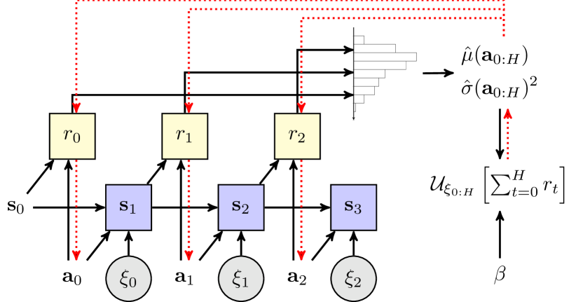
(a) RAPTOR-SLP

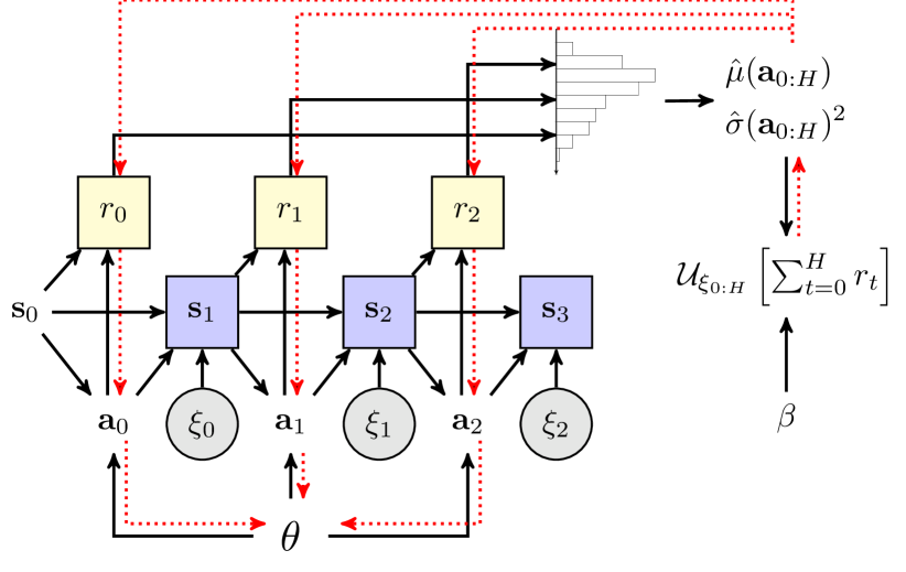
(b) RAPTOR-DRP

Figure 3: The stochastic computation graph of RAPTOR for three decision steps. Following Schulman et al. [28], square and rounded nodes show deterministic and stochastic nodes, respectively. The input nodes are drawn without borders. Note that all state nodes $\mathbf{s}_{1},\mathbf{s}_{2}\dots$ are deterministic due to the reparameterization via $\xi_{t}$. During the forward pass, the inputs of the model along with a batch of samples of $\xi_{t}\sim f_{\xi}$ induce an empirical distribution (histogram) over $\sum_{t=0}^{H}r(\mathbf{s}_{t},\mathbf{a}_{t})$. From this, we approximate the utility objective $\mathcal{U}$, which is a symbolic function of the samples and their sufficient statistics. We show the flow of gradients during backpropagation in red dotted lines.

4 Experiments

This section describes three domains which are used to analyze the performance of RAPTOR-SLP and RAPTOR-DRP. Additionally, the results and performance of RAPTOR are compared to risk neutral agents for each of the three domains.

4.1 Domain Descriptions

Navigation

Navigation [10] is a two-dimensional path-finding domain in which the goal is to find a shortest path from a fixed starting point to a fixed goal region. The continuous state $\mathbf{s}_{t}=(s_{t,x},s_{t,y})$ represents the location of the agent at time $t$ and the bounded continuous action $\mathbf{a}_{t}=(a_{t,x},a_{t,y})\in[-b,b]^{2}$ is the coordinate displacement of the agent at time $t$ for some $b>0$. The agent’s objective is to reach the goal region in a minimal number of time steps. Thus, the reward at each time step can be defined as the negative Euclidean distance from the agent to the center of the goal region $\mathbf{g}=(g_{x},g_{y})$, e.g. $r(\mathbf{s}_{t},\mathbf{a}_{t})=-\|\mathbf{s}_{t}-\mathbf{g}\|_{2}$. Notably, next state transitions are subject to high variability when the agent passes through a high-variance zone in between the starting point and the goal region. In particular, let $\mathrm{crossing}_{t}$ denote the length of a sub-trajectory that crosses the zone when moving from $\mathbf{s}_{t}$ to $\mathbf{s}_{t}+\mathbf{a}_{t}$. Then, a normally distributed noise $\mathcal{N}(0,(\mathrm{crossing}_{t}\sigma_{h})^{2})$ is added to the next state. On the other hand, when $\mathrm{crossing}_{t}=0$, a small noise $\mathcal{N}(0,\sigma_{l}^{2})$, whose variance $\sigma_{l}^{2}\ll\sigma_{h}^{2}$, is added. Thus, the transition function for the navigation domain can be reparameterized as:

$$\phi(\mathbf{s}_{t},\mathbf{a}_{t},\xi_{t})=\mathbf{s}_{t}+\mathbf{a}_{t}+\mathrm{crossing}_{t}\sigma_{h}\xi_{t}+\mathbbm{1}[\mathrm{crossing}_{t}=0]\sigma_{l}\xi_{t},\quad\xi_{t}\sim\mathcal{N}(\mathbf{0},\mathbf{I}_{2\times 2}).$$

Reservoir Control

The reservoir control domain [31] involves controlling the flow of water between $N=5$ interconnected reservoirs. The water level of each reservoir $i$ at time $t$ is represented by $s_{t,i}\in\mathbb{R}_{+}$. The action $a_{t,ij}=[\mathbf{a}_{t}]_{ij}$ is the amount of water discharged from reservoir $i$ to $j$ for $j\in\mathrm{downstream}(i)$, where $\mathrm{downstream}(i)$ is the set of downstream reservoirs of $i$ (we define $\mathrm{upstream}(i)$ similarly). The action is constrained such that $a_{t,ik}=0,\forall{k}\notin\mathrm{downstream}(i)$. Also, the total outflow of a reservoir cannot exceed the reservoir’s current water level, i.e., $\sum_{j}a_{t,ij}\leq s_{t,i}$. The goal of the agent is to keep the water level within a safe range $[L_{i},U_{i}]$, so we define the reward function as:

$$R_{i}\vcentcolon=\begin{cases}-P_{u}(s_{t,i}-U_{i}),&\text{if }s_{t,i}\geq U_{i}\\ -P_{l}(L_{i}-s_{t,i}),&\text{if }s_{t,i}\leq L_{i}\\ 0,&\text{otherwise}\\ \end{cases},\qquad r(\mathbf{s}_{t},\mathbf{a}_{t})=\sum_{i=1}^{N}R_{i},$$

where $P_{u}$ ($P_{l}$) is the penalty for water levels above (below) the upper (lower) bound. Note that $P_{u}$ is weighted more heavily than $P_{l}$, since overflows can lead to costly flooding and damages, whereas shortages can more easily be resolved by, e.g., supplementing water from secondary sources. The amount of rainfall at each time step is modelled as an exponentially-distributed random variable $\xi_{t}$ with rate $\lambda$. Thus, switching to a component-wise view of $\phi_{i}$ for notational clarity, the transition function for each reservoir $i$ becomes

$$\phi_{i}(\mathbf{s}_{t},\mathbf{a}_{t},\xi_{t})=s_{t,i}-\sum_{j\in\mathrm{downstream}(i)}a_{t,ij}+\sum_{j\in\mathrm{upstream}(i)}a_{t,ji}+\xi_{t}.$$

HVAC Control

In the HVAC control domain, an agent modulates the volume of heated air flow into each of the $N=5$ rooms in a house. The state consists of the temperature in each room $i$ given by $s_{t,i}\in\mathbb{R}$. The air volume, $\mathbf{a}_{t}$, into each room is non negative ($a_{t,i}\geq 0$) with constant temperature $T_{c}$. The objective is to keep the rooms at their set temperature and to avoid them getting too cold, so the reward function can be defined as:

$$R_{i}\vcentcolon=\begin{cases}-|s_{t,i}-T_{i}|-a_{t,i}-P_{u},&\text{if }s_{t,i}\leq T_{l}\\ -|s_{t,i}-T_{i}|-a_{t,i},&\text{otherwise}\\ \end{cases},\qquad r(\mathbf{s}_{t},\mathbf{a}_{t})=\sum_{i=1}^{N}R_{i},$$

where $T_{i}$ is the set temperature for room $i$, $T_{l}$ is a threshold on the temperature below which it would be considered too low, and $P_{u}$ is the penalty for the temperature going below $T_{l}$. As a cost saving measure, $T_{i}$ is set near $T_{l}$ to avoid expensive heating. Stochasticity is added in three ways for HVAC: (1) outdoor temperature is distributed as $\mathcal{N}(T_{o},\sigma_{o}^{2})$; (2) noise $\mathcal{N}(0,\sigma_{a}^{2})$ in the volume of air applied to each room; and (3) a small variance $\mathcal{N}(0,\sigma_{ij}^{2})$ in the heat dispersion between rooms. Combining this, the transition function for each room $i$ is:

$$\phi_{i}(\mathbf{s}_{t},\mathbf{a}_{t},\xi_{t})=s_{t,i}+a_{t,i}(T_{c}-s_{t,i})+\sigma_{a}\xi_{t}+\sum_{j\in\mathrm{Adjacent}(i)}\frac{(s_{t,j}-s_{t,i})^{3}}{\rho_{ij}}+\sigma_{ij}\xi_{t}+T_{o}+\sigma_{o}\xi_{t},$$

where $\xi_{t}\sim\mathcal{N}(0,1)$, $\rho_{ij}$ is the thermal resistance between adjacent rooms $i$ and $j$ and $\mathrm{Adjacent}(i)$ are the rooms adjacent to $i$.

4.2 Performance of Risk-Aware Planning

In this section, we analyze and compare the empirical performance of RAPTOR-SLP (RaSLP) and RAPTOR-DRP (RaDRP) against two recent scalable risk-neutral planners as baselines, the SLP approach in Wu et al. [30] and the DRP in Bueno et al. [4]. Please note that relevant hyper-parameters used in the experiments were tuned specifically for the baselines, with the exception of $\beta$, and used by RAPTOR for fair comparison (for detailed breakdown see Appendix A.3). The distributions of returns from all 3 domains are illustrated in Figure 4. Further analysis of the performance for different values of $\beta$ is provided in Appendix A.2.

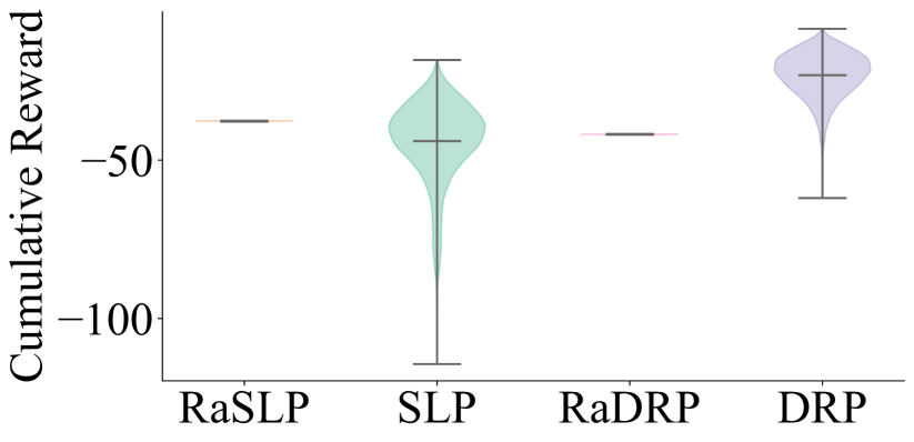
(a) Navigation

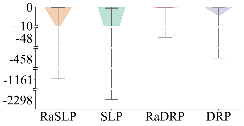
(b) Reservoir

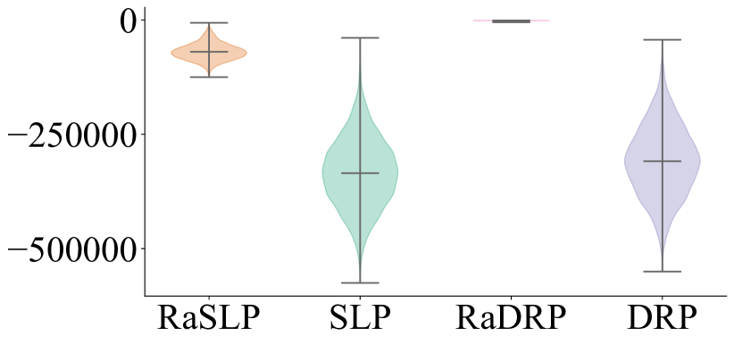
(c) HVAC

Figure 4: The cumulative reward distributions for all three domains are shown with SLP, RAPTOR-SLP, DRP and RAPTOR-DRP agents shown. To generate these distributions $10,\!000$, $250,\!000$ and $10,\!000$ trajectories were gathered for each agent in navigation, reservoir and hvac respectively.

Navigation Results

Figure 4(a) compares two RAPTOR agents against risk-neutral baselines. SLP achieves the lowest expected return as it cannot adapt to the highly stochastic environment and hence frequently fails to reach the goal region. DRP, on the other hand, attains the greatest expected return as it reactively approaches the goal region while passing through the high-variance zone (Figure 5). However, we can clearly see the advantage of risk-sensitive plans as they are able to obtain reasonably high returns while significantly reducing the variance in the returns at the same time. Figure 1 and Figure 5 show that RAPTOR agents circumvent the high-variance zone to reliably achieve high returns. Overall, the RAPTOR agents are unequivocally preferred in this domain when we have to avoid the worst-case outcomes.

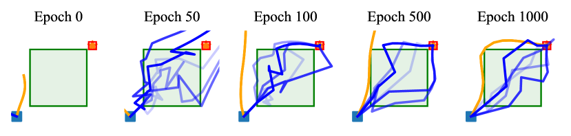
Figure 5: Similar to Figure 1, the evolution of trajectories of RAPTOR-DRP (orange) and a risk-neutral-DRP agent (blue) are shown.

Reservoir Results

We can see in Figure 4(b) that both RAPTOR agents have smaller variances in the return than their risk-neutral counterparts. Figure 6 shows that the optimized plan for the RAPTOR-SLP tends to maintain lower water levels than that for the SLP. Thus, RAPTOR agent is less likely to incur the large overflow penalty. Although DRP is able to attain smaller variance than RAPTOR-SLP by properly reacting to unveiled state transitions, further reduction in variance seen by RAPTOR-DRP is substantial. Also, we observe that the RAPTOR agents gain higher expected returns than the risk-neutral agents. This is because penalties are incurred only when the water levels go outside of the safe bounds; hence, keeping the levels within the bounds all the time ensures higher expected return as well. This shows the potential of RAPTOR in safety-critical applications.

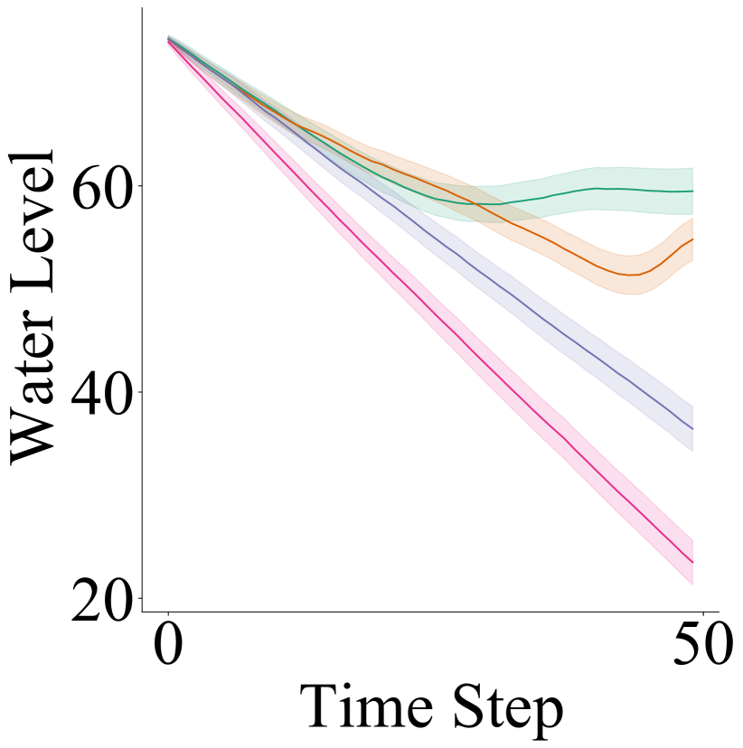
(a) Reservoir 1

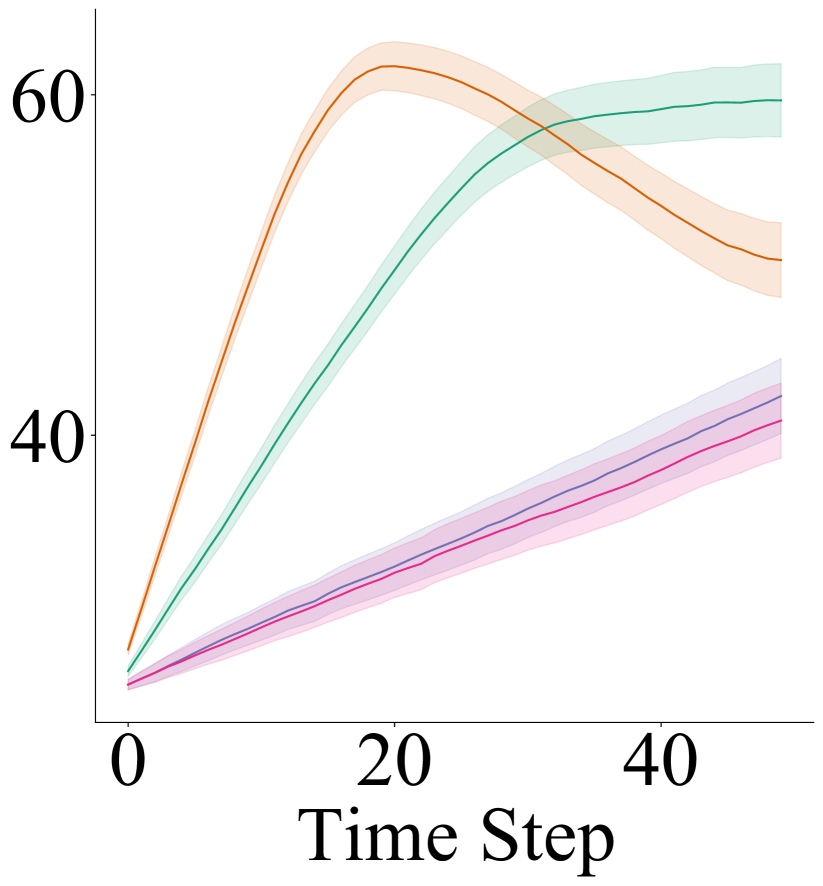
(b) Reservoir 2

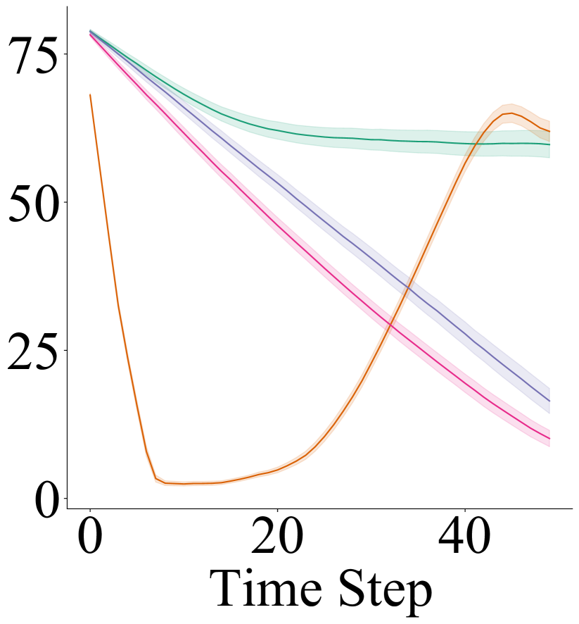
(c) Reservoir 3

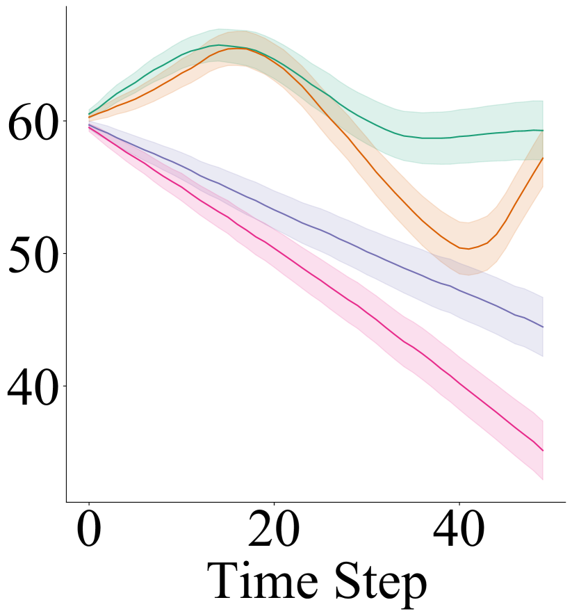
(d) Reservoir 4

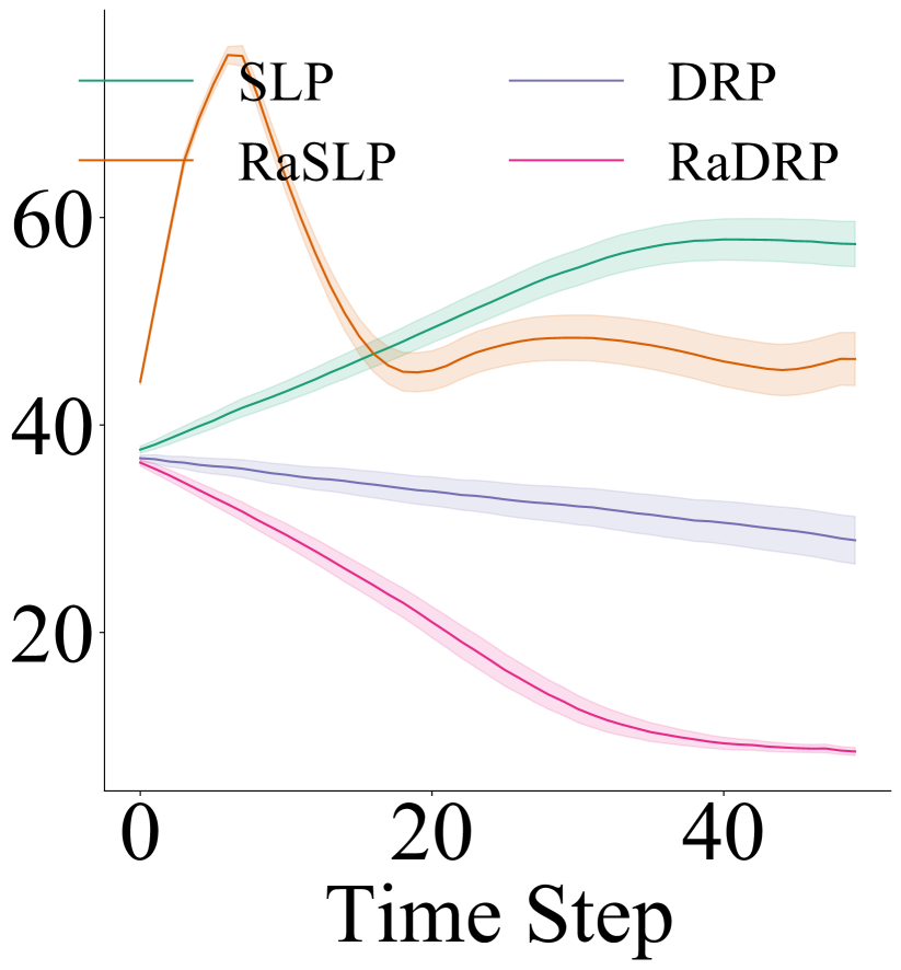
(e) Reservoir 5

Figure 6: The mean water levels and associated noise is shown for each of the five rooms with SLP, RAPTOR-SLP, DRP and RAPTOR-DRP.

HVAC Results

Figure 4(c) shows that both RAPTOR agents obtain lower variance in the return than their respective risk-neutral agents. RAPTOR-DRP accomplishes this by setting the room temperatures consistently high so that the penalty $P_{u}$ can be avoided at all times (Figure 7). Compared to RAPTOR-DRP, the optimized plan for RAPTOR-SLP induces more variability in the temperatures over time; however, the agent is still able to keep the temperatures from going below $T_{l}$ most of the times. In contrast, risk-neutral agents try to set the temperatures near $T_{l}$ to minimize the energy cost, which often leads to large penalties in this highly stochastic environment. Thus, the risk-neutral agents attain lower expected returns similar to the results in the Reservoir domain.

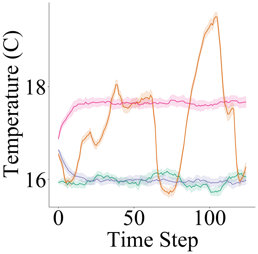
(a) Room 1

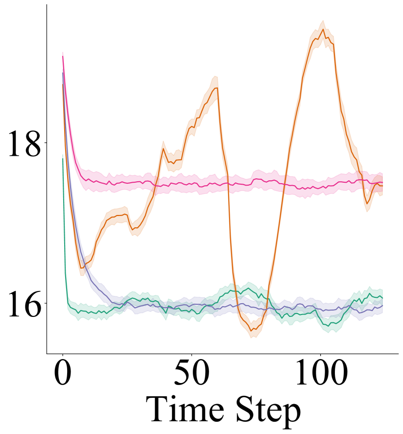
(b) Room 2

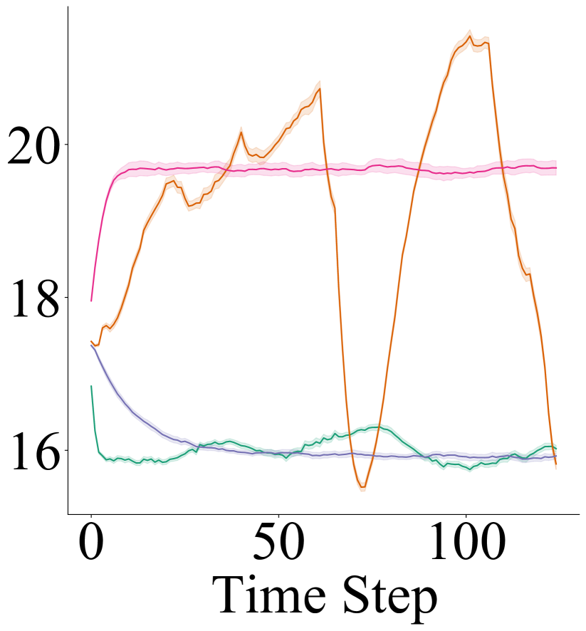
(c) Room 3

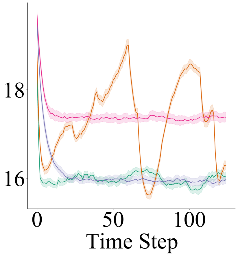
(d) Room 4

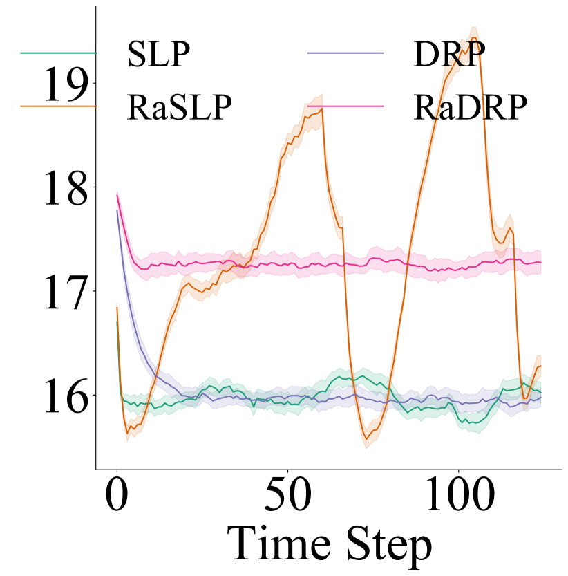
(e) Room 5

Figure 7: The mean room temperatures and associated noise is shown for each of the five rooms with SLP, RAPTOR-SLP, DRP and RAPTOR-DRP.

5 Conclusion and Future Work

We proposed RAPTOR, a scalable end-to-end risk-aware planner based on gradient descent applied to a risk-sensitive utility function. To this end, we extended BackpropPlan in order to accommodate stochastic transitions, by representing the planning problem as a stochastic computation graph and applying the reparameterization trick. Critically, we introduced the entropic utility as objective function, which can be seamlessly embedded in the graph as a symbolic objective. Then, risk-aware planning can be done end-to-end using an off-the-shelf automatic differentiation tool (e.g., PyTorch) by exploiting samples of the utility and their sufficient statistics. We applied these techniques to learn a straight-line plan which commits to a sequence of actions in advance, as well as deep reactive policies that can better adapt to highly stochastic environments. Experiments on three highly stochastic domains — Navigation, Reservoir, and HVAC – demonstrated the ability of RAPTOR to learn meaningful risk-sensitive policies in stochastic environments while maintaining scalability.

As future work, we note that extending our current approach to handle hybrid (mixed continuous and discrete) MDPs should be straightforward by using tricks such as projected gradients. Also, measuring and controlling risk is a complex topic in sequential decision making. The entropic utility objective and its mean-variance approximation may not capture all possible notions of risk. Applying this approach in situations such as financial portfolio optimization, where a model of dynamics is difficult to specify or even learn, and where the risk requirements could be potentially different, could lead to misrepresentation of risk. On the other hand, this could be addressed in different ways by using other well-known utility functions with different properties, such as CVaR [6]. However, this could be more difficult to incorporate into planning due to their reliance on percentiles of the return distribution and lack of asymptotic expansions exploited in this work. Incorporating other notions of risk could form an interesting and challenging future extension of our work. Another interesting extension could integrate model uncertainty for doing robust risk-aware planning under model misspecification.

Appendix A Appendix

A.1 Proof of Theorem 1

Let $\xi$ be a random variable, $A$ be an arbitrary set and $X_{a}=g_{a}(\xi)$ for $a\in A$ and some functions $g_{a}$. Since $\mathbb{P}\!\left(\sup_{a\in A}X_{a}\geq X_{b}\right)=1$ for every $b\in A$ and $\mathcal{U}_{\xi}\!\left(\cdot\right)$ is monotone, it follows that $\mathcal{U}_{\xi}\!\left(\sup_{a\in A}X_{a}\right)\geq\mathcal{U}_{\xi}\!\left(X_{b}\right)$. Since $b$ is arbitrary, we have $\mathcal{U}_{\xi}\!\left(\sup_{a\in A}X_{a}\right)\geq\sup_{a\in A}\mathcal{U}_{\xi}\!\left(X_{a}\right)$. Next, since $\mathbf{s}_{h+1}=\phi(\mathbf{s}_{h},\mathbf{a}_{h},\xi_{h})$, (5) and the monotonicity and translation invariance of $\mathcal{U}{}$:

$${U}^{*}_{0}\!\left(\mathbf{s}_{0}\right) =\sup_{\mathbf{a}_{0}}\,\mathcal{U}_{\xi_{0}}\!\left(r(\mathbf{s}_{0},\mathbf{a}_{0})+{U}^{*}_{1}\!\left(\mathbf{s}_{1}\right)\right)$$

$$=\sup_{\mathbf{a}_{0}}\,\mathcal{U}_{\xi_{0}}\!\left(r(\mathbf{s}_{0},\mathbf{a}_{0})+\sup_{\mathbf{a}_{1}}\,\mathcal{U}_{\xi_{1}}\!\left(r(\mathbf{s}_{1},\mathbf{a}_{1})+{U}^{*}_{2}\!\left(\mathbf{s}_{2}\right)\right)\right)$$

$$\geq\sup_{\mathbf{a}_{0}}\,\sup_{\mathbf{a}_{1}}\,\mathcal{U}_{\xi_{0}}\!\left(r(\mathbf{s}_{0},\mathbf{a}_{0})+\mathcal{U}_{\xi_{1}}\!\left(r(\mathbf{s}_{1},\mathbf{a}_{1})+{U}^{*}_{2}\!\left(\mathbf{s}_{2}\right)\right)\right)$$

$$=\sup_{\mathbf{a}_{0},\mathbf{a}_{1}}\,\mathcal{U}_{\xi_{0}}\!\left(\mathcal{U}_{\xi_{1}}\!\left(r(\mathbf{s}_{0},\mathbf{a}_{0})+r(\mathbf{s}_{1},\mathbf{a}_{1})+{U}^{*}_{2}\!\left(\mathbf{s}_{2}\right)\right)\right)$$

$$=\sup_{\mathbf{a}_{0},\mathbf{a}_{1}}\,\mathcal{U}_{\xi_{0},\xi_{1}}\!\left(r(\mathbf{s}_{0},\mathbf{a}_{0})+r(\mathbf{s}_{1},\mathbf{a}_{1})+{U}^{*}_{2}\!\left(\mathbf{s}_{2}\right)\right)$$

$$\geq\dots$$

$$=\sup_{\mathbf{a}_{0:H}}\,\mathcal{U}_{\xi_{0:H}}\!\left(r(\mathbf{s}_{0},\mathbf{a}_{0})+\dots+r(\mathbf{s}_{H},\mathbf{a}_{H})\right)$$

$$=u_{SL}(\mathbf{s}_{0}).$$

This completes the proof.

A.2 Additional Experiments

A.2.1 Varying Risk-Aversion

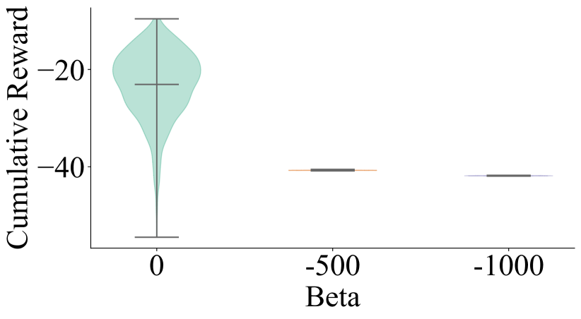
(a) Navigation

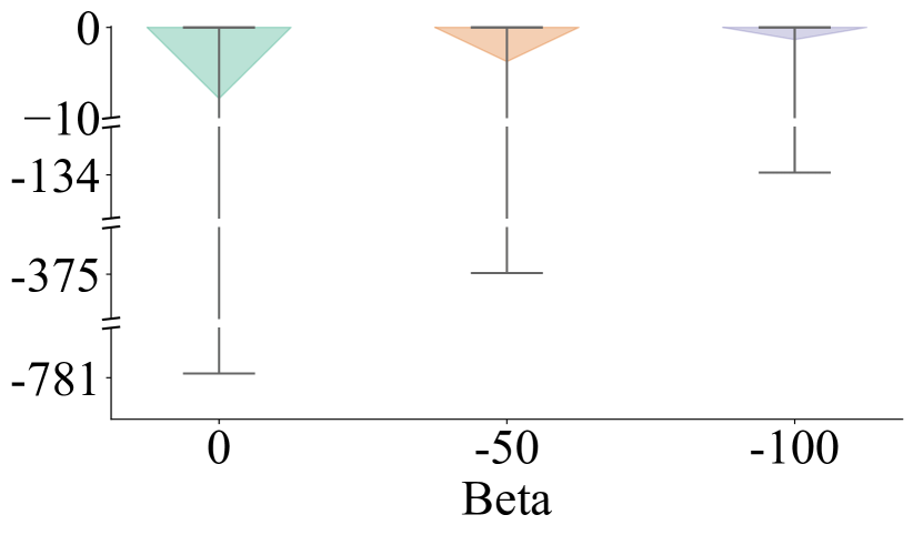
(b) Reservoir

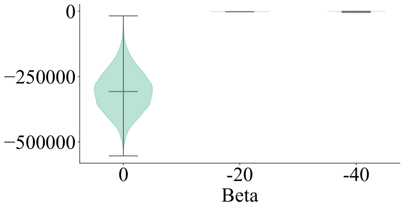
(c) HVAC

Figure 8: The cumulative reward distributions for RAPTOR-DRP over different values of the risk-aversion parameter $\beta$. Risk aversion increases from left to right.

In this section, we evaluate the performance of RAPTOR-DRP with varying values of the risk-aversion parameter $\beta$ in order to investigate its impact. Three levels of risk-averseness are chosen per each domain: risk-neutral, intermediate risk-aversion, and high risk-aversion. As in Section 4, we use the mean-variance approximation of the entropic risk (9) for all evaluations. Here, smaller $\beta$ (i.e., negative $\beta$ with large magnitude) represents greater risk-averseness.

In Figure 8, we can see that the $\beta$ parameter indeed gives us the control over how much risk-aversion we want an optimized policy to have. For Navigation and HVAC, we could obtain great reductions in the variances of cumulative rewards even with the intermediate $\beta$ values. In Reservoir, it is more apparent that RAPTOR-DRP with smaller $\beta$ values show more risk-averse behavior as represented by less variability in the corresponding returns. In general, the tradeoff is that we would attain a higher expected return yet a greater variance in returns with a higher $\beta$. However, DRP ($\beta=0$) gets lower expected returns in Reservoir and HVAC. As discussed in Section 4.2, this is because large penalties are incurred when visiting states that are outside of some bounds in these domains.

A.2.2 The Exact Entropic Risk Measure

In addition, we evaluate SLP, DRP, RAPTOR-SLP, and RAPTOR-DRP in all three domains using the exact entropic risk measure (2). Due to the well-known numerical instability of computation using the exact entropic risk [13], we are limited to $\beta$ with small magnitudes in these experiments: $\beta=-10^{-3}$ for Navigation and Reservoir, and $\beta=-10^{-4}$ for HVAC.

In Figure 9, we find similar patterns exhibited in Figure 4. That is, DRP performs better than SLP, and RAPTOR agents show smaller variance in returns than their risk-neutral counterparts. However, since we could only use the $\beta$ values with small magnitudes due to the aforementioned numerical instability, the reductions in variances are not significant when compared to the results in Figure 4. On the other hand, the results also indicate that it is possible to obtain comparable (for Navigation and Reservoir) or higher (for HVAC) expected returns with RAPTOR methods. When combined with the analysis in Appendix A.2.1, these results suggest that it is possible to find $\beta$ that is sufficiently small such that the expected return is not excessively penalized but is large enough to reduce the variance of returns. In conclusion, we note that higher-levels of risk-aversion would necessitate using the mean-variance approximation (as experimented in the main paper) due to its numerical stability across a wider range of $\beta$ values.

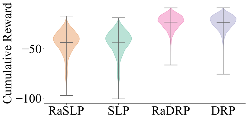
(a) Navigation

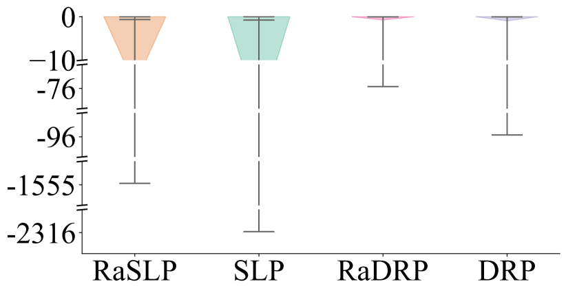
(b) Reservoir

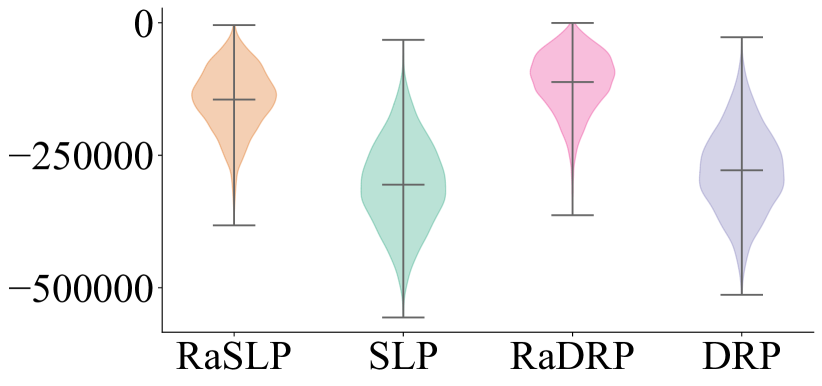
(c) HVAC

Figure 9: The cumulative reward distributions for SLP, RAPTOR-SLP, DRP and RAPTOR-DRP in all three domains using the exact entropic risk measure instead of the mean-variance approximation.

A.3 Experimental Setting Details

In this section, we provide a detailed accounting of the experimental parameters used in all experiments. All experiments were run on a single compute node with AMD Ryzen 7 4800H processor and NVIDIA GeForce RTX 2060 graphics card using PyTorch v1.7.1 and Python version 3.8.5. On this machine, compute time for each training run of a domain took less than 3 minutes. $\beta$ was chosen by iteratively increasing $\beta$ from $0$ until a significant reduction in variance was achieved for RAPTOR-SLP. The same $\beta$ was then used for RAPTOR-DRP to make for fair comparision.

Parameter	SLP	RAPTOR-SLP	DRP	RAPTOR-DRP
Learning Rate	$0.5$	$0.5$	$2.5*10^{-4}$	$2.5*10^{-4}$
Training Epochs	$1001$	$1001$	$1001$	$1001$
Batch Size	$8192$	$8192$	$8192$	$8192$
$\beta$	$0$	$-1000$	$0$	$-1000$
Time Horizon	$20$	$20$	$20$	$20$
Hidden-Layer-Nodes	N/A	N/A	$256,128,64,32$	$256,128,64,32$

Table 1: Hyperparameters of trained agents in the Navigation domain.

Parameter	SLP	RAPTOR-SLP	DRP	RAPTOR-DRP
Learning Rate	$0.2$	$0.2$	$5*10^{-3}$	$5*10^{-3}$
Training Epochs	$501$	$501$	$501$	$501$
Batch Size	$1024$	$1024$	$1024$	$1024$
$\beta$	$0$	$-100$	$0$	$-100$
Time Horizon	$50$	$50$	$50$	$50$
Hidden-Layer-Nodes	N/A	N/A	$256,128,64,32$	$256,128,64,32$

Table 2: Hyperparameters of trained agents in the Reservoir domain.

Parameter	SLP	RAPTOR-SLP	DRP	RAPTOR-DRP
Learning Rate	$5*10^{-3}$	$5*10^{-3}$	$5*10^{-3}$	$5*10^{-3}$
Training Epochs	$501$	$501$	$501$	$501$
Batch Size	$128$	$128$	$128$	$128$
$\beta$	$0$	$-40$	$0$	$-40$
Time Horizon	$125$	$125$	$125$	$125$
Hidden-Layer-Nodes	N/A	N/A	$256,128,64,32$	$256,128,64,32$

Table 3: Hyperparameters of trained agents in the HVAC domain.

References

- Bäuerle and Rieder [2014] Nicole Bäuerle and Ulrich Rieder. More risk-sensitive markov decision processes. Mathematics of Operations Research, 39(1):105–120, 2014.
- Blundell et al. [2015] Charles Blundell, Julien Cornebise, Koray Kavukcuoglu, and Daan Wierstra. Weight uncertainty in neural network. In ICML, volume 37 of PMLR, pages 1613–1622. PMLR, 07–09 Jul 2015.
- Boutilier et al. [1999] Craig Boutilier, Thomas Dean, and Steve Hanks. Decision-theoretic planning: Structural assumptions and computational leverage. J. Artif. Int. Res., 11(1):1–94, July 1999. ISSN 1076-9757.
- Bueno et al. [2019] Thiago P Bueno, Leliane N de Barros, Denis D Mauá, and Scott Sanner. Deep reactive policies for planning in stochastic nonlinear domains. In AAAI, volume 33, pages 7530–7537, 2019.
- Burns et al. [2012] Ethan Burns, J Benton, Wheeler Ruml, Sungwook Yoon, and Minh Do. Anticipatory on-line planning. In ICAPS, volume 22, 2012.
- Chow et al. [2015] Yinlam Chow, Aviv Tamar, Shie Mannor, and Marco Pavone. Risk-sensitive and robust decision-making: a cvar optimization approach. In NeurIPS, 2015.
- Defourny et al. [2008] Boris Defourny, Damien Ernst, and Louis Wehenkel. Risk-aware decision making and dynamic programming. 2008.
- Dowson et al. [2020] Oscar Dowson, David P Morton, and Bernardo K Pagnoncelli. Multistage stochastic programs with the entropic risk measure, 2020.
- Faria [2018] José Faria. Machine learning safety: An overview. Safety-critical Systems Symposium 2018 (SSS’18), 02 2018.
- Faulwasser and Findeisen [2009] Timm Faulwasser and Rolf Findeisen. Nonlinear model predictive path-following control. Nonlinear Model Predictive Control - Towards New Challenging Applications, pages 335–343, 2009. URL http://infoscience.epfl.ch/record/184946.
- Figurnov et al. [2018] Mikhail Figurnov, Shakir Mohamed, and Andriy Mnih. Implicit reparameterization gradients. In NeurIPS, volume 31, 2018.
- Föllmer and Schied [2002] Hans Föllmer and Alexander Schied. Convex measures of risk and trading constraints. Finance and stochastics, 6(4):429–447, 2002.
- Gosavi et al. [2014] Abhijit A Gosavi, Sajal K Das, and Susan L Murray. Beyond exponential utility functions: A variance-adjusted approach for risk-averse reinforcement learning. In 2014 IEEE Symposium on Adaptive Dynamic Programming and Reinforcement Learning, pages 1–8. IEEE, 2014.
- Issakkimuthu et al. [2015] Murugeswari Issakkimuthu, Alan Fern, Roni Khardon, Prasad Tadepalli, and Shan Xue. Hindsight optimization for probabilistic planning with factored actions. In ICAPS, volume 25, 2015.
- Kingma and Welling [2014] Diederik P. Kingma and Max Welling. Auto-Encoding Variational Bayes. In ICLR, 2014.
- Kupper and Schachermayer [2009] Michael Kupper and Walter Schachermayer. Representation results for law invariant time consistent functions. Mathematics and Financial Economics, 2(3):189–210, 2009.
- Maccheroni et al. [2006] Fabio Maccheroni, Massimo Marinacci, and Aldo Rustichini. Ambiguity aversion, robustness, and the variational representation of preferences. Econometrica, 74(6):1447–1498, 2006.
- Mannor and Tsitsiklis [2011] Shie Mannor and John N Tsitsiklis. Mean-variance optimization in markov decision processes. In ICML, pages 177–184, 2011.
- Mercier and Van Hentenryck [2008] Luc Mercier and Pascal Van Hentenryck. Amsaa: A multistep anticipatory algorithm for online stochastic combinatorial optimization. In International Conference on Integration of Artificial Intelligence (AI) and Operations Research (OR) Techniques in Constraint Programming, pages 173–187. Springer, 2008.
- Moldovan [2014] Teodor Mihai Moldovan. Safety, risk awareness and exploration in reinforcement learning. PhD thesis, University of California, Berkeley, 2014.
- Osogami [2012] Takayuki Osogami. Robustness and risk-sensitivity in markov decision processes. NeurIPS, 25:233–241, 2012.
- Paszke et al. [2019] Adam Paszke, Sam Gross, Francisco Massa, Adam Lerer, James Bradbury, Gregory Chanan, Trevor Killeen, Zeming Lin, Natalia Gimelshein, Luca Antiga, Alban Desmaison, Andreas Kopf, Edward Yang, Zachary DeVito, Martin Raison, Alykhan Tejani, Sasank Chilamkurthy, Benoit Steiner, Lu Fang, Junjie Bai, and Soumith Chintala. Pytorch: An imperative style, high-performance deep learning library. In NeurIPS, pages 8024–8035. 2019.
- Pereira and Thomas [2020] Ana Pereira and Carsten Thomas. Challenges of machine learning applied to safety-critical cyber-physical systems. Machine Learning and Knowledge Extraction, 2, 11 2020. doi: 10.3390/make2040031.
- Puterman [2014] Martin L Puterman. Markov decision processes: discrete stochastic dynamic programming. John Wiley & Sons, 2014.
- Raghavan et al. [2017] Aswin Raghavan, Scott Sanner, Roni Khardon, Prasad Tadepalli, and Alan Fern. Hindsight optimization for hybrid state and action mdps. In AAAI, volume 31, 2017.
- Ruiz et al. [2016] FJR Ruiz, MK Titsias, and DM Blei. The generalized reparameterization gradient. NeurIPS, pages 460–468, 2016.
- Ruszczyński [2010] Andrzej Ruszczyński. Risk-averse dynamic programming for markov decision processes. Mathematical programming, 125(2):235–261, 2010.
- Schulman et al. [2015] John Schulman, Nicolas Heess, Theophane Weber, and Pieter Abbeel. Gradient estimation using stochastic computation graphs. In NeurIPS, page 3528–3536, 2015.
- Tieleman and Hinton [2012] T. Tieleman and G. Hinton. Lecture 6.5—RmsProp: Divide the gradient by a running average of its recent magnitude. COURSERA: Neural Networks for Machine Learning, 2012.
- Wu et al. [2017] Ga Wu, Buser Say, and Scott Sanner. Scalable planning with tensorflow for hybrid nonlinear domains. In NeurIPS, 2017.
- Yeh [1985] William W-G Yeh. Reservoir management and operations models: A state-of-the-art review. Water resources research, 21(12):1797–1818, 1985.