Certification of embedded systems based on Machine Learning: A survey

Abstract.

Advances in machine learning (ML) open the way to innovating functions in the avionic domain, such as navigation/surveillance assistance (e.g. vision-based navigation, obstacle sensing, virtual sensing), speech-to-text applications, autonomous flight, predictive maintenance or cockpit assistance. Current certification standards and practices, which were defined and refined decades over decades with classical programming in mind, do not however support this new development paradigm. This article provides an overview of the main challenges raised by the use ML in the demonstration of compliance with regulation requirements, and a survey of literature relevant to these challenges, with particular focus on the issues of robustness and explainability of ML results.

1. Introduction

Safety critical systems, and avionics in particular, represent an application field unenthusiastic in applying new software development methods (Krodel, 2008), as shown by the fact that some aspects of the object-oriented programming, such as polymorphism and dynamic biding, never made their way to safety critical systems, mostly because the inconvenient balance between added value and increased development and validation costs. Nevertheless, the recent advances in machine learning triggered genuine interest, as machine learning offer promising preliminary results and open the way to a wide range of new functions for avionics systems, for instance in the area of autonomous flying. In this paper we investigate on how existing certification and regulation techniques, can (or cannot) handle software development that includes parts obtained by machine learning.

Nowadays a large aircraft cockpit offers many avionic complex functions: flight controls, navigation, surveillance, communications, displays… Their design has required a top down iterative approach from aircraft level downward, thus the functions are performed by systems of systems, with each system decomposed into subsystems that may contain a collection of software and hardware items. Therefore, any avionic development considers 3 levels of engineering: (i) Function, (ii) System/Subsystem and (iii) Item. The development process of each engineering level relies on several decades of experience and good practices that keep on being adapted today. These methods have been standardized through EUROCAE/SAE standards for system development (ED-79A/ARP4754A) and EUROCAE/RTCA standards for software items (ED-12C/DO-178C and supplements) and hardware items (ED-80/DO-254). They are recognized as applicable means of compliance with regulation requirements by worldwide Avionic Authorities (AAs). In this context, this survey actually reduces the domain of study to the item level and more precisely to the software item. Note that at the item level, the correct terminology for the demonstration of conformity to standards is “qualification”.

The item’s development workflow is usually represented by the V-cycle (refer to Figure 1). Today, the usual development paradigms are Requirement-based Engineering (RBE) or Model-Based Engineering (MBE). Indeed, avionic items are developed using classical programming, i.e. the developers explicitly use language instructions to implement requirements (or model) and thus are able to control each line of code of the embedded software item.

Recently, new avionic functions have emerged, aiming at developing new flight experiences: navigation/surveillance assistance (e.g. vision-based navigation, obstacle sensing, virtual sensing), speech-to-text applications, autonomous flight, predictive maintenance, cockpit assistance…

Contrary to classical programming which can hardly support these functions, Machine Learning (ML) which is a sub-domain of Artificial Intelligence (AI), is well known to show good results for most of them (e.g. (Bahdanau et al., 2015; Devlin et al., 2019; Redmon et al., 2016)). Current industrial guidance have a strong focus on bespoke technologies in aeronautical applications thus, are not appropriate to support this paradigm change.

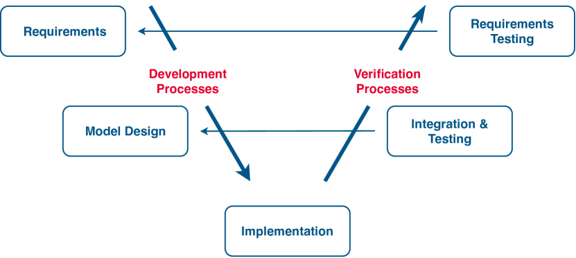
Figure 1. Item development workflow

Indeed, ML techniques introduce a brand new paradigm in avionic development: the data-driven design of models (including supervised, unsupervised and reinforcement learning). Data-driven refers to the fact that the data rule the algorithm behavior through a learning phase. We choose to restrict our research to offline supervised learning, i.e. the training is done with labelled data and before embedding the ML software. As a first step to the qualification of a ML item, these restrictions seems reasonable. Besides, these restrictions do not affect our capability to find efficient algorithms that might solve the emerging functions mentioned above.

Even with this restriction, many significant issues remains regarding the current demonstration of conformity. Indeed, some fundamentals of the usual techniques (Requirement Based Engineering or Model Based Engineering) are jeopardized, challenging the classical safety guarantee argumentation:

• Specifiability: It sounds difficult, a priori, to capture the complete behavior of a ML model (for instance when the training dataset is composed of millions of images), decreasing the confidence that the model behaviour will always match the functional intent and be free of unintended behavior that may jeopardize the safety.

• Traceability: The relationship between item requirements and corresponding learned parameters of the ML algorithm cannot be established. This makes the ML item design less transparent and draw a need for explainability capabilities to add confidence that the algorithm correctly and safely implements the intended function.

• Robustness: Perturbations in the design phase and the operational inference of the trained algorithm may lower the reliability on the predictions correctness and may degrade the functional and safety performances.

The motivation of this survey is two-fold: (i) identify the main challenges to the certification of ML based item (see Figure 2), (ii) overview the literature to know whether existing methods or techniques are able to solve the problems raised by the identified challenges. Compared with the survey of Huang et al. (2020), which is also motivated by the certification of critical embedded systems that include Deep Neural Network (DNN), our survey is guided by aeronautics regulations and standards and is not limited to DNN, although many of the cited works deal with DNN.

Currently, the challenges for certifying ML algorithms are listed in Figure 2. The goal of this survey is not to provide a complete overview of possible techniques to solve these challenges, its scope is reduced to the trustworthiness and methodology considerations. Specifically, the survey focuses on Explanability and Robustness (more precisely adversarial robustness) because they address key issues introduced by the intrinsic characteristics of ML algorithms: the lack of transparency of the design (black-box aspect) and the lack of performances reliability when inputs are slightly perturbed in the range of the Operational Design Domain (ODD). In grey, in Figure 2, are the topics that are out of our scope: Embeddability and Resiliency. Embeddability raises classical implementation concerns such as the deterministic behavior of the item versus memory and computational constraints. Some resolution techniques are specific to ML, such as the optimization of the ML algorithm structure or implementation architecture to fit the targeted host platform. Resiliency monitors the behavior of the system when it is deployed, e.g. error detection or fault tolerance. This is an issue to be addressed at the system level of engineering.

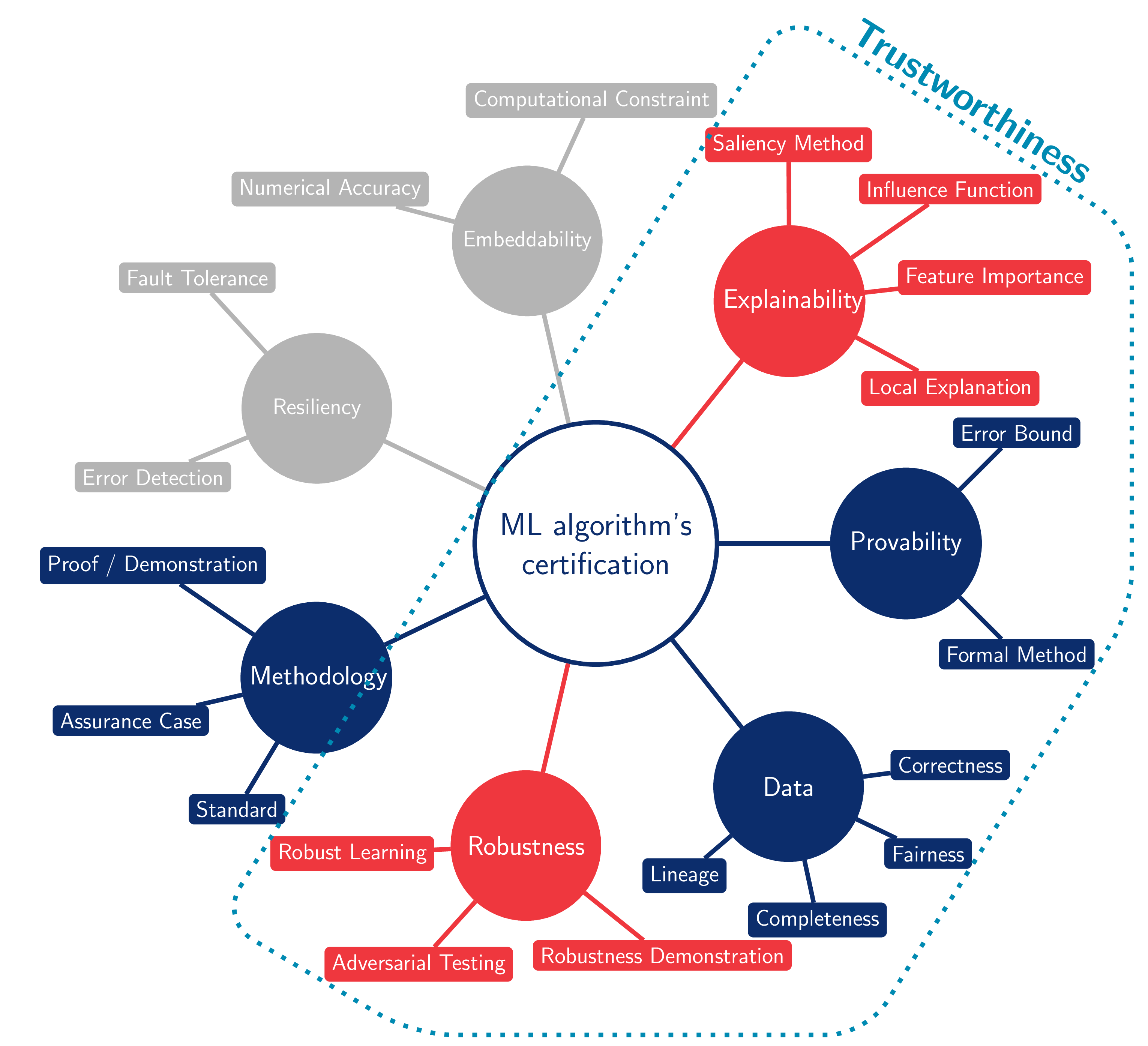
Figure 2. AI certification key elements. In red, are the domain that we detail in this survey. In blue are the domain that we briefly present. In grey are the domain out of our scope.

This paper is structured as follows: in section 2, we overview the main challenges raised by the use ML in the demonstration of compliance with regulation requirements. In section 3 we introduce the Trustworthiness considerations which will possibly help to fill the existing gaps in future certification approaches (see Figure 3). Then the sections 4 and 5 focus on robustness and explainability, respectively. Eventually, we end the paper with section 6 which recaps the identified problems for the qualification of ML items.

2. Impact of ML techniques on certification approach

The European Union Aviation Safety Agency (EASA) provides regulatory material that defines and explains all the requirements due for developing safe avionic products (EASA, 2018). Regarding software/hardware items embedded in avionic safety-related systems, the certification specification are described in CS 2x.1301 and CS 2x.1309. Roughly speaking, we would summarize these paragraphs as follows: avionic systems should safely perform their intended function under all foreseeable operating and environmental conditions. Through supplemental documents (AMC20-115D and AMC20-152A), EASA recognizes the current avionic standards as acceptable means of compliance to the regulation text. The grey element in Figure 3 shows the relation between regulations and standards.

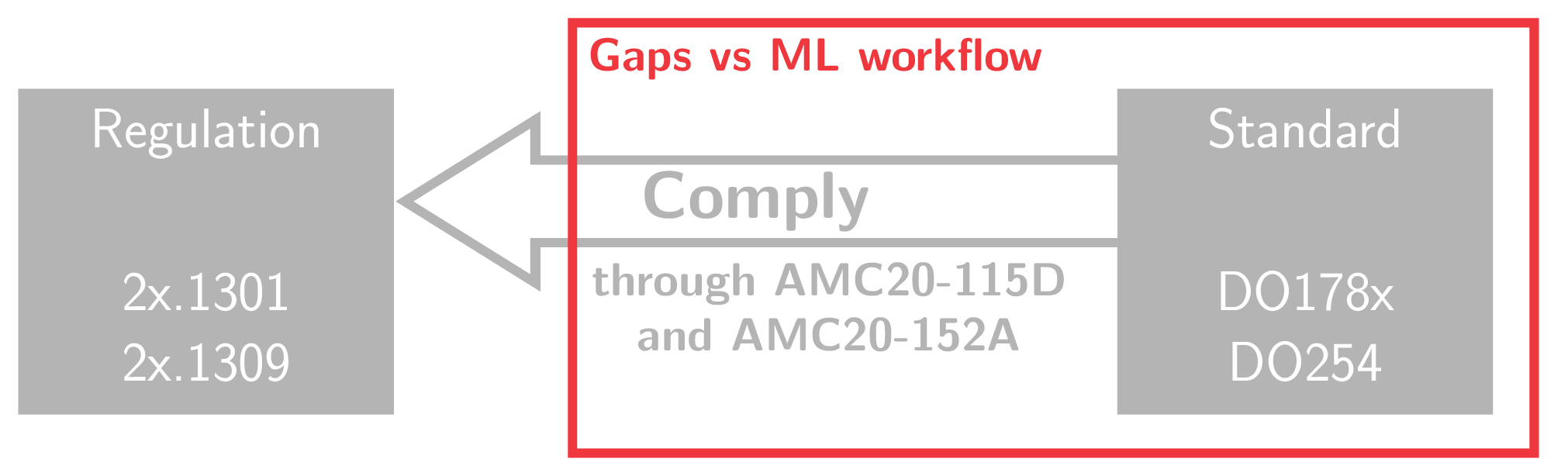
Figure 3. Certification Process Overview

Assuming the ML techniques are reduced to offline learning, we do not anticipate any change to the regulation (EASA, 2018). However, even if regulation requirements are unchanged, the current standards do not provide sufficient guidance to make a complete demonstration of conformity for a ML item. This section details these gaps.

Specifiability

One of the fundamentals of the RBE (or MBE) relies on the correct and complete capture of the item requirements: either they come from system allocated requirements (intent) or from its own behavior (emerging functions). In this context, the item can be verified to safely perform the intended function under all foreseeable operating and environmental conditions. With ML items, it sounds difficult to fully specify the function with a classical requirement process. For instance, all the possible way to describe a runway whatever the operational (e.g. sensors own bias) and the environment conditions (e.g. weather, light conditions) cannot be defined using textual or even modelling technique. This is the reason why we will prefer use millions of images instead, betting that the data experience will complete the requirement capture and that ML technique will enable the development of an acceptable runway detection function. Therefore the difficulty will be to describe as thoroughly as necessary the operational domain (ODD) in which the detection function is supposed to operate and then to validate that the collected data correctly and sufficiently represent this ODD.

Traceability

The current software standard requires the traceability between the requirements and the code (in both senses) so that each line of embedded code can be justified as implementing captured requirements. In a ML development context, this relationship that makes the design a white-box process, is lost. Actually the trained algorithm is a complex mathematical expression (made of arithmetic operations with weights and bias) that is not traceable to any upward functional requirements. Thus it becomes infeasible to demonstrate the completeness of implementation using traceability. From this lack of traceability comes the loss of transparency of the model, making the link from the input data to the output predictions not understandable by a human. This lowers the confidence that the safety properties of the intended function are preserved in its operational domain. In this context, explainable AI could be a means to enhance the confidence in these algorithms when safety is highly critical (see section 3 and 5).

Unintended behaviour

All the life-cycle processes (requirements capture, model design, implementation, integration and requirement-based testing) of the item development workflow (see Figure 1) are used to demonstrate the consistency with the intended function. In addition to the problems mentioned above, the learning phase could introduce some unexpected behavior that we cannot measure or prevent using usual activities. It means that we cannot guarantee the absence of unintended behavior during item operation and specifically those affecting aircraft safety. This may be due to several root causes such as a low-quality data management process (e.g. bias, mislabeled data) or inadequate learning process. We will see in the rest of the paper that there are methods to limit or to formally verify the occurrence of such effects.

3. Trustworthiness Considerations

The qualification of ML items in the frame of avionic developments offers lots of research challenges in various domains. We selected the overview of 5 different domains that seem very promising and which will contribute to support the certification of ML-based systems. Thus, this section overviews the domains covering the Trustworthiness (see Figure 2) and the Methodology aspects.

Explainability and robustness of Machine Learning model have already been reviewed, the reader may therefore refer to (Huang et al., 2020; Biggio and Roli, 2018; Ren et al., 2020), to get more details on these topics. Nevertheless, the originality of our work stands in the perspective of the conformity to the regulation requirements inherent to the development of safety-critical systems for avionic domain.

Explainability

Explainability is a topic inherent to ML technique. It is not needed for classical programming since the item development can be fully explained through the joint requirement and traceability processes which enable the interpretation of each line of embedded code. ML development breaks this understanding chain and make room for an undesirable black box effect. This is the reason why one can think that, when required by the safety level of the implemented function, explainability would be requested to add the necessary confidence to support the demonstration of conformity (EASA, 2020). Phillips et al. (2020) introduce four principles of explainable AI: explanation, meaningfulness, explanation accuracy, knowledge limits. Basically, these principles state that an explainable AI must: (i) provide an “evidence or reason for all outputs” (ii) be meaningful with respect to the audience, (iii) be representative of the way that the algorithm produce the output and (iv) be aware of the domain of usage of the algorithm, i.e. it should not give an explanation when the input is out of scope since the algorithm is not design to work with it.

In the aeronautical context, four stakeholders could need explanation: the designer, the authorities, the pilot and the investigator. Considering the “meaningfulness” principle, each of them could receive different explanation. Indeed, the needs for explanation would be different for an engineer who knows the system and for an end-user who has no prior knowledge of the system. The explanations could also differ whether it is used for debugging purposes during the development (for designer), for investigation purposes in case of in-flight issues (for authorities or investigator) or for a user assessment of the model predictions when the system is deployed, e.g. a pilot who requests justification of the decision to enhance his confidence in the system before acting. In the literature, we find two kinds of explanation: local explanation (Guidotti et al., 2018; Ribeiro et al., 2016, 2018; Dabkowski and Gal, 2017; Fong and Vedaldi, 2017; Hendricks et al., 2016; Kendall and Gal, 2017; Zeiler and Fergus, 2014) and global explanation (Lundberg and Lee, 2017; Shrikumar et al., 2017; Zhao and Hastie, 2019) (see Section 5).

Adversarial Robustness

Robustness comprises several sub-domains (adversarial examples, distributional shift, unknown classes, physical attacks, …) but we focus only on adversarial robustness which is defined as the capability of algorithms to give the same outputs considering some variation of the inputs in a region of the state space. The issues addressed by the adversarial robustness domain are at the heart of the certification process; it addresses partially the demonstration of the intended function. The aim is to assess and/or enhance the behavior of the algorithm when dealing with abnormal inputs (noise, corner case, sensor malfunction…). The literature is two sided: one side works at enhancing the adversarial robustness of the algorithm (Carlini et al., 2019; Gilmer et al., 2019; Goodfellow et al., 2015; Kurakin et al., 2017b; Madry et al., 2018; Papernot et al., 2016; Papernot and McDaniel, 2018; Szegedy et al., 2014; Zhang et al., 2019), the other side at its verification (Cissé et al., 2017; Gehr et al., 2018; Huang et al., 2017; Katz et al., 2017; Koh and Liang, 2017; Mirman et al., 2018; Salman et al., 2019; Singh et al., 2019; Tsuzuku et al., 2018). Improving the adversarial robustness consists in finding robust learning procedure that is resilient against crafted exampled made to defeat the ML algorithm. The verification of this latter property is either based on formal methods (Cissé et al., 2017; Koh and Liang, 2017; Salman et al., 2019; Tsuzuku et al., 2018; Katz et al., 2017) or optimization methods (Gehr et al., 2018; Huang et al., 2017; Mirman et al., 2018; Singh et al., 2019).

Provability

The provability aspect is the capability to formally demonstrate that system properties are preserved. Formal methods provides mathematical evidences to support such demonstration. As stated above, formal methods are already used to verify well-defined properties of algorithms (Katz et al., 2017; Katz et al., 2019; Wang et al., 2018), such as the robustness (Huang et al., 2017; Gehr et al., 2018; Mirman et al., 2018; Singh et al., 2019).

The error (or generalization) bound gives guarantees on the ability of the algorithm to generalize.. An algorithm generalizes well when it maintains its high performance on unseen data, i.e. the theoretical error, $r$ is close to the empirical error $\hat{r}_{S}$ (computed from a training set $S$). The idea is to bound the gap between the theoretical error $r$ and its empirical counterpart $\hat{r}_{S}$. However, $r$ is not computable since it is the error on all possible data. Hence, the need for probabilistic bounds which give an upper bound on the gap between $r$ and $\hat{r}_{S}$. The first generalization bounds appears with the PAC (Probably Approximately Correct) theory (Valiant, 1984) and have the following forms:

(1) $$\text{Pr}_{S}\Big{(}|r-\hat{r}_{S}|\leq\epsilon(\text{model's complexity},\#S,\delta)\Big{)}\geq 1-\delta,$$

where $\epsilon(\cdot)\geq 0$ and $\delta\in\left]0,1\right]$. $\epsilon$ is a function that models the upper bound that usually relies on the complexity of the model, the number of samples in $S$ (denoted by $\#S$), and the probability $\delta$. The ideal scenario is to have the gap between $r$ and $\hat{r}_{S}$ small while having a high probability that the inequality holds, i.e. having $\epsilon(\cdot)$ and $\delta$ as small as possible.

Particularly, the PAC-Bayesian theory(McAllester, 1999; Shawe-Taylor and Williamson, 1997), which interprets an algorithm as a majority vote, is well known to provide tight generalization bound (Parrado-Hernández et al., 2012). A majority vote is defined as the weighted sum of several models where the weights of the sum constitute a distribution $Q$. Hence, a model follows a prior distribution $P$ before the learning and posterior distribution $Q$ after. A PAC-Bayesian generalization bound could have the following form:

(2) $$\text{Pr}_{S}\Big{(}r\leq\hat{r}_{S}+\epsilon(KL(Q\|P),\#S,\delta)\Big{)}\geq 1-\delta.$$

One can notice that both bounds have a similar structure but the particularity of the PAC-Bayesian theory is to use the Kullback-Leibler divergence between $Q$ and $P$ to quantify the complexity of the model. Besides, the differences stand also in the definition of $r$ and $\hat{r}_{S}$ since in the PAC-Bayesian theory the algorithm is interpreted as a majority vote.

Data management

In the avionic context, data has been used for a long time with the use of databases or configuration files. However Machine Learning techniques are bringing a totally new aspect in the qualification approach. Contrary to classical programming, ML design techniques are data-driven, thus the data management process is essential to the demonstration of conformity. As already stated, building a ML algorithm of good quality, requires data of good quality (no erroneous data, no mislabelled data, …) but this is not sufficient. Indeed the data representativeness plays also a significant role. Representativeness comes from statistics and is a quite challenging problem: it allows to check if the data is a correct snapshot of the phenomenon to be learnt.

The quality of the data can be measured using existing metrics: accuracy, consistency, relevance, timeliness, traceability, and fairness are some of them (Cai and Zhu, 2015; Picard et al., 2020). Accuracy checks if the data is well measured and stored. Consistency verifies if the preprocessing of the data does not compromise their integrity. Relevance measures if there are sufficient data to learn the intended function and if the data contain the correct information regarding the needs. Timeliness concerns the availability of the data over time. Traceability verifies the reliability of the data source and if all activities for the transmission do not alter the data integrity. Fairness is about avoiding undesirable bias in the dataset.

Methodology

The methodology structures the assurance activities that are needed to support the qualification aspects, i.e. the demonstration to the Authorities that the item development is compliant with the standardized guidance. The red square in Figure 3 highlights that changes are required in the AMCs and/or the industrial standards. Therefore it will be necessary to find alternative means to comply with the regulation material, either by adapting the current certification approach or by building a new one.

Then it will be crucial to clearly define the development process of ML items ((Baylor et al., 2017; Ashmore et al., 2019; Amershi et al., 2019; Studer et al., 2020)) to (i) ease their development and maintainability, and (ii) identify the validation and verification activities. Figure 4 describes this development process: requirements from the system/subsystem level are refined into ML item requirements to fit to the three main stages of the workflow: Data Management process, Design process and Implementation process.
Data Management Process First data are collected with respect to the problem to be solved. Then, the data should be cleaned and labelled, i.e. inaccurate data samples are removed and each remaining data sample is assigned with a true label (known as “ground truth”). Finally, data are preprocessed and split. Preprocessing encompasses all the tasks that transform the data into a more suitable format for the design phases (e.g. feature engineering or data normalization). Preprocessing effort may vary depending on the data collection phase (e.g. data comes from different sources) and the type of data (e.g. images, time series, tabular, sound, text). After the preprocessing step, the data is split into a training, a validation and a testing dataset.
Design Process The design process takes as input the three datasets and outputs a frozen model. The processes in this stage are more iterative than sequential. To tune the hyper-parameters of a model, you iterate between the training and the validation phase. After the tuning part, you are able to test your model. If the performances are lower than expected with respect to the ML item requirements, it is possible to loop back either to the data management process or the design process.
Implementation Process Within the implementation stage, the specificity of the hardware is taken into consideration: the frozen model is optimized and converted with respect to the host platform constraints and the operational requirements cascaded from the system level. Finally, a binary code is generated and loaded in the hardware target. Since we only consider the item design aspects, the implementation stage is out of the scope of this survey.

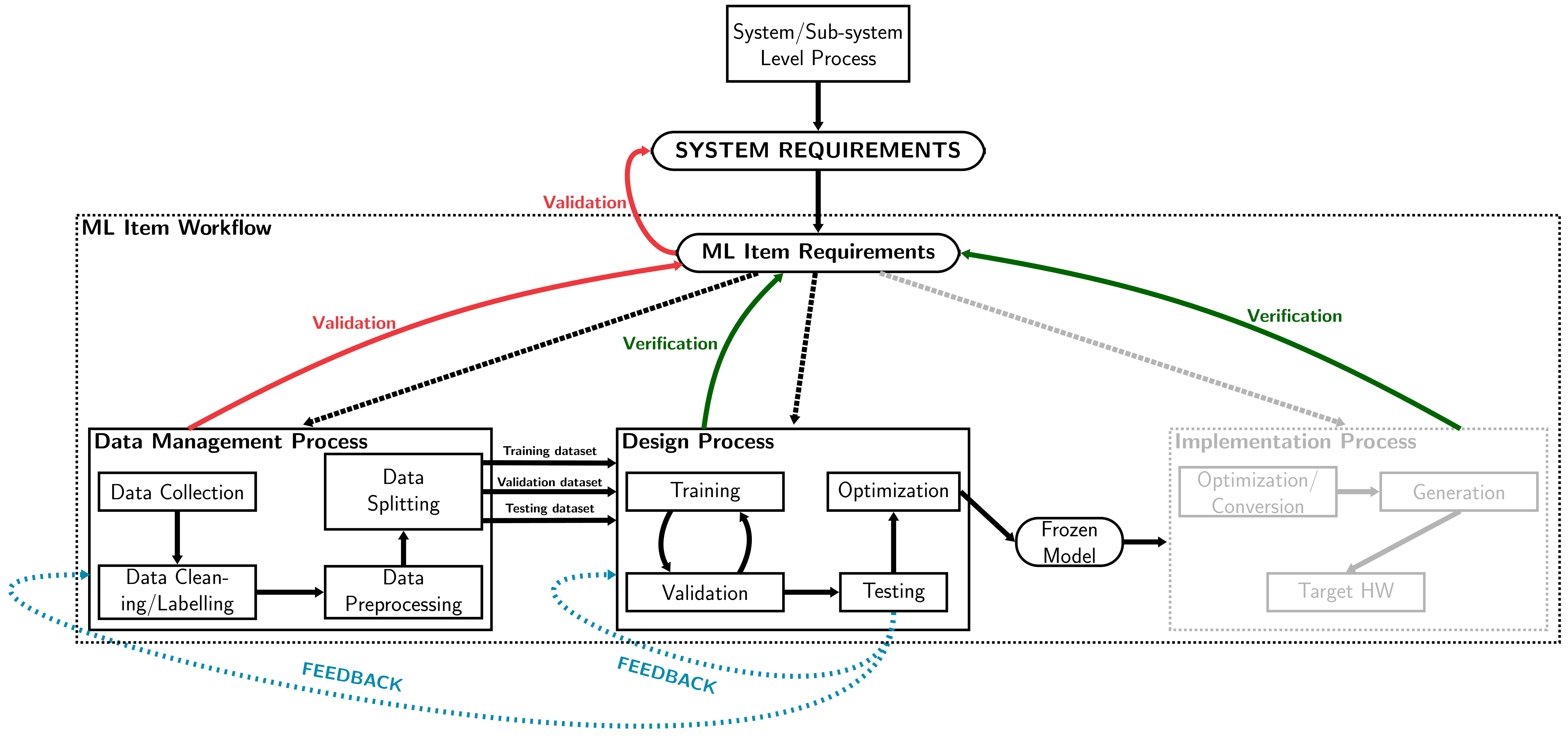
Figure 4. Machine Learning development process: The three main stages of ML development process (Data Management Process, Design Process and Implementation Process). The stage in grey is out of the survey scope. The red arrows show the validation activities. The green arrows show the verification activities. The blue arrows show where we can loop back if the model underperforms.

Since its creation in the 80’s, the ED-12/DO-178 standard issues gather the industrial best practices that impose the necessary rigor of development to avoid the introduction of errors that may lead to a system failure, and thus increase the safety of the system. Historically, methodologies undeniably brought efficient results in terms of safety. Thus methodological considerations are key to build a correct certification approach. One lead to build relevant safety argumentation is the concept of safety case (Rushby, 2015) or assurance case (Martin, 2017). Indeed, Rushby (2015) argues that the introduction of this kind of methodology (i.e. not prescriptive approaches) in the industries helps to significantly reduce the number of accidents and deaths. Assurance cases, which are a generalization of safety cases, are defined by MITRE (Martin, 2017) as follows: a documented body of evidence that provides a convincing and valid argument that a specified set of critical claims regarding a system’s properties are adequately justified for a given application in a given environment. Hence, assurance cases could be used during the development process of a ML-based item to build, share and discuss sets of structured arguments to support the demonstration of conformity based on outcomes of specific assurance techniques.

4. Adversarial Robustness

Table 1. Summary of robustness method: The top of the table shows the papers that provide an attack and/or a defense and the bottom shows the papers that provide a verification method. The $\ell_{p}$-norm column refers the norm originally considered in the papers to compute the distance between $x$ and $x_{adv}$. “-” means that the method do not rely on an $\ell_{p}$-norm. The color code indicate whether the norm is used for attack or defense; black means it is used for both. The colunm “# parameters” reports the size of the Neural Network (in terms of numbers of parameters) used in the papers; it give an insight on the scalability of the associated method.

Attack/Defense
Method Name	Papers	Attack	Defense	$\ell_{p}$-norm
c&w	Carlini and Wagner (2017)	✓		$\ell_{0}$/$\ell_{2}$/$\ell_{\infty}$
parseval training	Cissé et al. (2017)		✓	$\ell_{2}$
fgsm	Goodfellow et al. (2015)	✓	✓	$\ell_{\infty}$
ifgsm	Kurakin et al. (2017b)	✓	✓	$\ell_{\infty}$
gradient-based attack+ila ((Huang et al., 2019))	Li et al. (2020)	✓∗		$\ell_{\infty}$
pgd	Madry et al. (2018)	✓	✓	$\ell_{\infty}$/$\ell_{2}$
deepfool	Moosavi-Dezfooli et al. (2016)	✓		$\ell_{2}$
jsma	Papernot et al. (2016)	✓		$\ell_{0}$
dknn	Papernot and McDaniel (2018)	✓∗	✓	$\ell_{\infty}$/$\ell_{2}$
l-bfgs	Szegedy et al. (2014)	✓	✓	$\ell_{2}$
lmt	Tsuzuku et al. (2018)		✓	$\ell_{2}$
gda	Zantedeschi et al. (2017)		✓	-
yopo	Zhang et al. (2019)		✓	$\ell_{\infty}$
Verification
Method Name	Papers	Sound	Complete	# paramaters
ai2	Gehr et al. (2018)	✓		$>$ 238,000
dlv	Huang et al. (2017)	✓	✓	$>$ 138,000,000
reluplex	Katz et al. (2017)	✓	✓	$\sim$ 13,000
marabou	Katz et al. (2019)	✓	✓	$\sim$ 13,000
refinezono	Singh et al. (2019)	✓		$>$ 1,000,000
reluval	Wang et al. (2018)	✓

^∗ The authors adapt existing attacks to target the weakness of their defense.

Concerning the fundamentals of the regulation requirements, i.e. mainly to demonstrate that the system safely performs the intended function, the key role of robustness is twofold: on one hand and according to ED-12C/DO-178C, it is the extent to which software can continue to operate correctly despite abnormal inputs and conditions. On the other hand and more specifically to ML application, EASA (2020) states that ML system is robust when it produces the same outputs for an input varying in a region of the state space. Perturbations can be natural (e.g. sensor noise, bias…), variations due to failures (e.g. invalid data from degraded sensors) or maliciously inserted (e.g. pixels modified in images) to fool the model predictions. When perturbed examples fool the ML algorithm we talk about adversarial examples. It is commonly defined as noises on inputs that are imperceptible or that do not exceed a threshold. We state in Definition 4.1 two possible manners of generating adversarial examples, i.e. attacking an ML model.

Definition 4.1.

Adversarial Example. Let $(x,y)$ be a benign example and the true label, $\delta$ be a perturbation, $\epsilon$ be the maximum allowed perturbation, $L$ be a loss function and $f$ be the trained ML model, we have
$\displaystyle\min\|\delta\|_{p}$ (3) such that $\displaystyle f(x+\delta)\neq y,$ $\displaystyle x+\delta\in Domain(x)$ or $\displaystyle\max L(f(x+\delta),y)$ (4) such that $\displaystyle\|\delta\|_{p}\leq\epsilon,$ $\displaystyle x+\delta\in\text{Domain}(x)$  
where $\|\cdot\|_{p}$ is an $\ell_{p}$-norm and Domain($x$) depict the allowed values for the example $x$.

As stated in Definition 4.1 the optimization problem leads to get an adversarial example with a different label than the original one; we refer to it as “untargeted attack”. Few modifications of the optimization problem allow to have a “targeted attack”, i.e. the possibility to choose the label of the adversarial examples. Let $t$ be the targeted label we have,
$\displaystyle\min_{\delta}\|\delta\|_{p}$ such that $\displaystyle f(x+\delta)=t,$ $\displaystyle x+\delta\in Domain(x)$ or $\displaystyle\min_{\delta}L(f(x+\delta),t)$ such that $\displaystyle\|\delta\|_{p}\leq\epsilon,$ $\displaystyle x+\delta\in\text{Domain}(x)$ .

Moreover, the attacks could be done in either a white-box or black-box setting. White-box setting basically means that the attacker has full access to the model, its parameters and the training dataset while black-box setting means that the attacker can only query the model with data.

Finally, the means deployed to overcome adversarial attacks is known as adversarial defenses. One of the most efficient defense is the Adversarial Training (AT) (Goodfellow et al., 2015; Kurakin et al., 2017b; Madry et al., 2018). It consists in augmenting your training dataset with adversarial examples. However, it is often observed that the adversarial training based on a particular $\ell_{p}$-norm are less effective against attacks based on different $\ell_{p}$-norm.

Nevertheless, the defenses only enhance the adversarial robustness of ML algorithms whereas for the demonstration of conformity, we will need proof that systems based on the ML algorithm behave safely and as expected. Actually, there exists methods in the literature that verify that an ML algorithm is adversarially robust. It could bring the guarantee needed to demonstrate the conformity to the regulation requirement. Thus, to handle the adversarial robustness issue, we review adversarial attacks/defenses (cf. Section 4.1) and verification methods (cf. Section 4.2). We report in table 4 adversarial attacks/defenses and verification methods. It is important to highlight that, for the attack/defense methods, we report the $\ell_{p}$-norm used in the paper. However the methods could be adapted to other norms.

4.1. Adversarial attacks/defenses

Szegedy et al. (2014) was one of the first to point out adversarial examples as a weakness of ML algorithm. The highlighting of this weakness gave rise to numerous researches around adversarial attacks and defenses (Gilmer et al., 2019; Kurakin et al., 2017b; Gourdeau et al., 2019; Szegedy et al., 2014; Papernot et al., 2016; Goodfellow et al., 2015; Koh and Liang, 2017; Kurakin et al., 2017a; Madry et al., 2018; Papernot and McDaniel, 2018; Zhang et al., 2019). Carlini et al. (2019) provide advice and good practices about the evaluation of the adversarial robustness. Especially, they claim that one that develops a new defense mechanism must think about an “adaptive attack” to evaluate the efficiency of their defense mechanism. In other words, to evaluate the defense efficiency of your new defense mechanism, you have to test the worst attack against it.

4.1.1. Attack

Goodfellow et al. (2015) develop an efficient method to find adversarial example called Fast Gradient Sign Method (fgsm). The attack consists in crafting the adversarial example $x_{adv}$, by adding a fraction, $\epsilon$, of the loss gradient’s sign with respect to the input to the original example $x$:

$$x_{adv}=x+\epsilon\cdot\text{sign}(\nabla_{x}L(f(x),y)).$$

Besides, the authors show that adversarial examples are invariant to the learning and the architecture, i.e. different architecture trained on different subsets of the dataset misclassify the same adversarial example. Later, Kurakin et al. (2017b) propose an iterative version of fgsm which we denote ifgsm where at each iteration, a perturbation is added to $x$ by applying fgsm to finally obtain $x_{adv}$ after the desired number of iterations:

$$x_{adv}^{0}=x\qquad x_{adv}^{i}=x_{adv}^{i-1}+\epsilon\cdot\text{sign}(\nabla_{x}L(f(x_{adv}^{i-1}),y)).$$

Since perturbations are added several times to $x$ in ifgsm, the $\epsilon$ chosen is therefore smaller than in fgsm. The attack introduced by Madry et al. (2018) based on Projected Gradient Descent (pgd) is similar to ifgsm except that pgd randomly initialize $x$ before the optimization:

$$x_{adv}^{0}=x+noise\qquad x_{adv}^{i}=x_{adv}^{i-1}+\epsilon\cdot\text{sign}(\nabla_{x}L(f(x_{adv}^{i-1}),y)).$$

Carlini and Wagner (2017) also develop a gradient based method but with a slightly different formulation of the optimization problem (cf. Definition 4.1). It is similar to Equation 4.1 but at the same time they minimize the margin of the model. Besides, the authors provide the formulation of their method for three distance metrics ($\ell_{0}$, $\ell_{2}$ and $\ell_{\infty}$). Moosavi-Dezfooli et al. (2016) tailor their attack framework, called deepfool, for finding the minimum perturbation necessary with respect to the $\ell_{2}$-norm to fool the algorithm. They first simplify the optimization problem to a linear classifier, derive the optimal solution for it and finally adapt the optimal solution found for the linear classifier to neural network. They provide the algorithm of deepfool which describe their iterative approach to estimate the smallest perturbation to create an adversarial example (cf. Algorithm 2 of (Moosavi-Dezfooli et al., 2016)). Their results show that the adversarial example crafted by deepfool is often closer to the original example than the ones crafted by fgsm and l-bfgs (Szegedy et al., 2014).

Papernot et al. (2016) leverage the “forward derivative” of a network $f$, to design the Jacobian-based Saliency Map Attack (jsma). To obtain the forward derivative, they compute, from the input layer to the output layer, the derivative of the network $f$, instead of the derivative of its loss function, with respect to the input $x$. It basically corresponds to the Jacobian of the function learned by the network $f$. Then, the authors derive a “adversarial saliency map” based on the Jacobian of the network which points out the input feature that should be modified in order to get a significant impact on the network’s output. We refer the reader to their paper (Papernot et al., 2016) to get more detail on the algorithm they provide to craft an adversarial example using forward derivative and adversarial saliency map.

Kurakin et al. (2017a) assess the adversarial robustness of models deployed in “real-world conditions”, i.e. the only way to communicate with the systems is through its sensors. Indeed this is a legitimate question since an attacker will not necessarily have access to the ML model. In their experiments, the authors feed an image classification algorithm through a camera. However, they still use the model to generate adversarial examples. They demonstrate that models are still vulnerable against adversarial attack even in “real-world conditions”.

In the avionic context, security mesure will be taken to restrict the access to the models and the datasets to undermine the white-box and black-box attacks. Nevertheless the threat still exists since Li et al. (2020) propose an attack in a more restricted setting than black-box known as “no-box” setting (Chen et al., 2017) where the attacker only have very few number of examples that are not training examples. They succeed to efficiently fool the models trained on the imagenet dataset by developing an auto-encoder called “prototypical reconstruction” that manages to learn well with very few data. An auto-encoder consists of two parts: an encoder and a decoder. The encoder, encodes the input by learning a new representation of the original input and the decoder strives to reconstruct the input from the encoding as close as possible to the original input. The authors introduce a new loss for their auto-encoder that is well suited for gradient based attack. Then, their attack consists in using ILA (Huang et al., 2019), which improves the transferability of the attack, in addition to the gradient-based method.

4.1.2. Defense

As stated earlier, one of the most effective defense, called Adversarial Training (AT), consists in replacing your original training dataset by an “adversarial dataset” crafted with an attack. However, this method is time consuming, since it requires to generate adversarial example at each step of the learning phase. Nevertheless, Goodfellow et al. (2015) overcome this issue with fgsm and propose an adversarial training where they replace a part of the training dataset with perturbed example. Following this principle, other works with stronger attacks propose adversarial training based on these attacks (Kurakin et al., 2017b; Madry et al., 2018). Besides, Madry et al. (2018) show that the adversarial training principle boils down to solve the following min-max optimization (or saddle-point problem):

(5) $$\min_{\theta}\operatorname*{\mathbb{E}}_{(x,y)\sim\mathcal{D}}\left[\max_{\|\delta\|_{p}\leq\epsilon}L(f_{\theta}(x+\delta),y)\right],$$

where $\mathcal{D}$ is the unknown distribution of the dataset, $f_{\theta}$ is the model whose parameters is $\theta$, $L$ is the loss and $\epsilon$ is maximum allowed perturbations. Indeed, the equation 5 comprises two parts: maximization and minimization. On the one hand, the equation maximizes the loss regarding the noises $\delta\leq\epsilon$, i.e. it makes $x+\delta$ more likely to be an adversarial example. On the other hand, the equation minimizes the expectation of the loss regarding the model’s parameters. To the best of our knowledge, AT based on pgd is one of the most efficient defense against attacks using the $\ell_{\infty}$-norm.

Though the methods presented above make AT feasible, it still increase the learning time of a model. Zhang et al. (2019) aim at improving the computation cost of AT by reformulating it as a differential game and then derive the Pontryagin’s Maximum Principle (PMP). The PMP reveals that AT are closely linked with the first layer of neural networks. Therefore they develop yopo (You Only Propagate Once) which leverage this fact by limiting the number of forward and backward propagation without worsening the network’s performance. Their experiments show that yopo learn $4$ to $5$ time faster to achieve as good results as adversarial training based on pgd.

Papernot and McDaniel (2018) find another mean to enhance the robustness of ML algorithms. The authors develop a method called Deep k-Nearest Neighbors (dknn), i.e. a hybrid classifier that mixes Deep Neural Network (DNN) and kNN. Their motivation is to improve the confidence estimation, the model interpretability, and the robustness. The principle of dknn is to find the nearest neighbors (from the training set) of an input $x$ at each layer of the DNN and find the classes of each neighbor. This procedure allows the analysis of the evolution of classes in the neighborhood of $x$ throughout the network. That is why, the authors introduce several metrics such as nonconformity and credibility. The nonconformity metric is used to measure the discrepancy between the labels of the neighborhood and the predicted label of an input $x$. A high nonconformity value means that the labels predicted for the neighborhood of $x$ is different from the one predicted for $x$. The computation of the credibility measure is based on “calibration dataset” whose examples were not used for the training. Then, the credibility of an input $x$ is the ratio of nonconformity measures of the examples from the calibration dataset that are greater than the input’s nonconformity measure. dknn increases the confidence in predictions thanks to the credibility measure which is used to assess and select model’s predictions. Moreover, this algorithm becomes more interpretable because of the neighborhood it provides which gives an insight of its “internal work”. Papernot and McDaniel (2018) claim that dknn would prevent adversarial examples by assigning to them a low credibiility measure. Their empirical results show particular encouraging results against c&w attack.

The drawback of the above techniques lies on their dependence to the $\ell_{p}$-norm. Indeed, even if it brings robustness against attacks relying on the same metric distance (like pgd), the defense could become ineffective when the attacks depend on a different metric distance. Instead of searching for the perturbation that maximizes the loss function of a model (Equation 5), Zantedeschi et al. (2017) propose to consider all the local perturbations (drawn from a gaussian distribution) around each examples:

$$\min_{\theta}\operatorname*{\mathbb{E}}_{(x,y)\sim\mathcal{D}}\;\operatorname*{\mathbb{E}}_{\delta\sim\mathcal{N}(0,\sigma^{2})}L(f_{\theta}(x+\delta),y),$$

where $\mathcal{D}$ is the unknown distribution of the dataset, $f_{\theta}$ is the model whose parameters is $\theta$ and $L$ is the loss function of the model. They claim that their method, known as Gaussian Data Augmentation (gda), instead of crafting adversarial example only in the direction of the gradient, explore much more directions around the examples. gda outperforms AT considering adversarial accuracy measure (i.e. accuracy on a attacked dataset) on MNIST (LeCun et al., 1998) and CIFAR-10 (Krizhevsky, 2009).

A hypothesis that could explain the adversarial phenomenon is the high expressiveness of the models, i.e. the the capacity of the model to learn complex behavior. Cissé et al. (2017) and Tsuzuku et al. (2018) explore this lead by constraining the Lipschitz constant of neural networks to enhance their robustness. Considering all possible couple of points of the input space of a function $f$, the Lipschitz constant is the smallest value that upperbound the absolute value of the slopes given by each pair of points. Intuitively, we would say that constraining the Lipschitz constant of a function $f$ to a small value would smooth the function and therefore reduce its expressiveness. Cissé et al. (2017) develop specific training called parseval training which consists in ensuring that the Lipschitz constant of all the network’s layers is smaller than $1$ by having Parseval tight weight’s matrices. We refer interested readers to the paper (Cissé et al., 2017) for the mathematical details. Tsuzuku et al. (2018) propose another training method, called Lipschitz Margin Training (lmt), to constrain the Lipschitz constant of a network. They first link the margin of network to the Lipschitz constant. From that, they derive an algorithm relying on the relation between the margin and the Lipschitz constant that enhance the robustness of the network. Besides, lmt provide a “certified” lower bound on the smallest perturbation that can defeat the network. This latter property could be desirable for the demonstration of conformity to the regulation requirement of an embedded system based on ML. Indeed, theoretical results are great assets for the certification process. For example, Gourdeau et al. (2019) leverage the PAC theory (Probably Approximately Correct) to provide theoretical proof of the feasibility of robust learning from the perspective of computational learning theory. The authors focus on the setting where the input space is the boolean hypercube $\mathcal{X}=\{0,1\}^{n}$ and show that robust learning is feasible or not for different classes of models.

Remark

Gilmer et al. (2019) conduct experiments showing that improving adversarial robustness also improve corruption robustness, i.e. the robustness of the model against distributional shift. They want to show that both type of robustness could be the manifestation of the same phenomenon. Nevertheless, it is encouraging that improving adversarial robustness has a positive impact on corruption robustness.

4.2. Verification

The existing frameworks for verifying ML models show that is possible to verify many types of property as long as you are able to express it in the manner expected by the verification framework. However, the literature focuses on a specific property which is the robustness. For that reason we decided to distinguish 4.2.1 Properties Verification and 4.2.2 Robustness Verification. Basically, there are two important criteria for a verifier: completeness and soundness. Completeness means that the verifier can verify all the properties that hold whereas soundness means that the verifier cannot prove any wrong property.

4.2.1. Properties Verification

Some methods in the literature claim to do property verification (Katz et al., 2017; Katz et al., 2019; Wang et al., 2018). As stated earlier, verifying that the desired properties hold for an ML algorithm presupposes that we can express them as expected by the verifier, i.e. in the format that verifier could verify.

Katz et al. (2017) develop a method that uses Simplex algorithm —a method to solve optimization problem of linear programming— and Satisfiability Modulo Theories solver (SMT solver) —a solver for formulas of first-order logic with respect to some background theories such as arithmetic, arrays, …— which the authors adapt to work with Neural Network using specific activation function (ReLU: $y=max(0,x)$). Their method is called reluplex and they run it on a case study: ACAS XU system. They use quantifier-free formulas to the formalization of properties which consists in constrained domains for inputs and outputs. Basically, they reduce the verification problem into a constraint satisfiability problem (CSP). They verified 10 properties with reluplex and got a timeout for 2 of them, i.e. reluplex was not able to end the verification within the given time. The longest verification took almost 5 days while the fastest took less than 8 minutes. marabou (Katz et al., 2019), which is the successor of reluplex, is based on the same principles. The framework, now supports piecewise linear layer and activation and has a “divide and conquer mode” which improves the computation time of the verification.

4.2.2. Adversarial Robustness Verification

Robustness verification is an emerging field (Cissé et al., 2017; Gehr et al., 2018; Gourdeau et al., 2019; Huang et al., 2017; Singh et al., 2019; Tsuzuku et al., 2018). Verifying robustness means ensuring that the algorithm outputs the same label $y$ for an example $x$ and its neighborhood whose the computation usually rely on metric distance (e.g. $\ell_{p}$-norm) This property could be stated as follow:

(6) $$\forall x^{\prime}\;\text{s.t.}\;\|x-x^{\prime}\|_{p}\leq\epsilon,\quad f(x)=f(x^{\prime}),$$

where $\|x-x^{\prime}\|_{p}\leq\epsilon$ represent the neighborhood around $x$ such that the distance between $x$ and any neighbor $x^{\prime}$ does not exceed $\epsilon$ and $f$ is the ML model. Indeed, the existence of adversarial examples could be seen as the negation of Equation 6. Thus, verifying that Equation 6 holds boils down to check the adversarial robustness of an algorithm.

Singh et al. (2019) develop refinezono, a verification framework mixing optimization techniques (MILP, LP/MILP relaxation) and abstract interpretation —a method mainly use in static analysis that leverage overappromixation to analyse the behavior of computer programs—. Mixing those techniques allows better scalability for complete verifiers and improves the precision of incomplete ones. The principle of refinezono is to compute the boundaries of the neurons using optimization techniques and abstract interpretation. As in (Katz et al., 2017), a property is expressed as domains for inputs and outputs. A robustness property expressed as same label predicted whatever the point within a region around $x$ can be easily transformed into domains for input and output: the region around $x$ is the domain for the input and the domain for the output is given to have the right class. For example, Figure 5 shows a robustness property where we verify that in the neighborhood of the point $x=(0.9,0.7,0.4)$ the model outputs only the desired class (the output layer predict always the same class).

Instead of trying to scale up to complete verifiers, such as MILP, with abstract interpretation (Singh et al., 2019), it is possible to make abstract interpretation as precise as possible (Gehr et al., 2018). The benefit of applying only abstract interpretation is to verify properties on large neural networks (e.g. CNN). Gehr et al. (2018) develop ai² framework which implements abstract interpretation techniques to verify neural networks. Their framework also focus on the verification of the robustness property (Equation 6). In ai²(Gehr et al., 2018), the input is replaced by an abstract domain then it is propagated through the network thanks to abstract transformers until the output layer. Property verification is applied to the abstract domain obtained at the output layer. The method is sound but incomplete, meaning that for a property the result can either be true or inconclusive. Hence the choice of the abstract domain for the input is important because it influences the precision of the verifier.

Huang et al. (2017) reduce the proof of robustness to a search of adversarial examples. They focus on the robustness of image classification which is a quite hard problem considering the possible input domain of an image and all perturbation it can have. The first assumption is that images are discrete. Therefore, Huang et al. (2017) explore completely the region of an image $x$, searching for an adversarial example, by defining a set of minimum manipulation. To develop a verification procedure that ensures the safety of a point, the authors first formally define a safe point. Based on their assumption of “discrete images”, the authors develop an algorithm of safety verification using SMT solvers; their tool is called Deep Learning Verification (dlv). Since the method of (Huang et al., 2017) is sound and complete, if the algorithm does not find any adversarial example, it means that there are none for the region and the manipulation set considered. Moreover, Huang et al. (2017) show that their algorithm is scalable to big neural networks by doing experiments on neural networks with more than one hundred million of parameters.

Xu et al. (2020) provide a framework, named lirpa, that unifies the methods of linear relaxation whose goal is to find affine functions that upperbound and lowerbound the output of the network. For example, to prove a robustness property (as stated in Equation 6) with lirpa, we must show that the lower bound of the true label is greater than alll upper bounds of all other classes; this would mean that in the worst case, the model will always output the correct class.

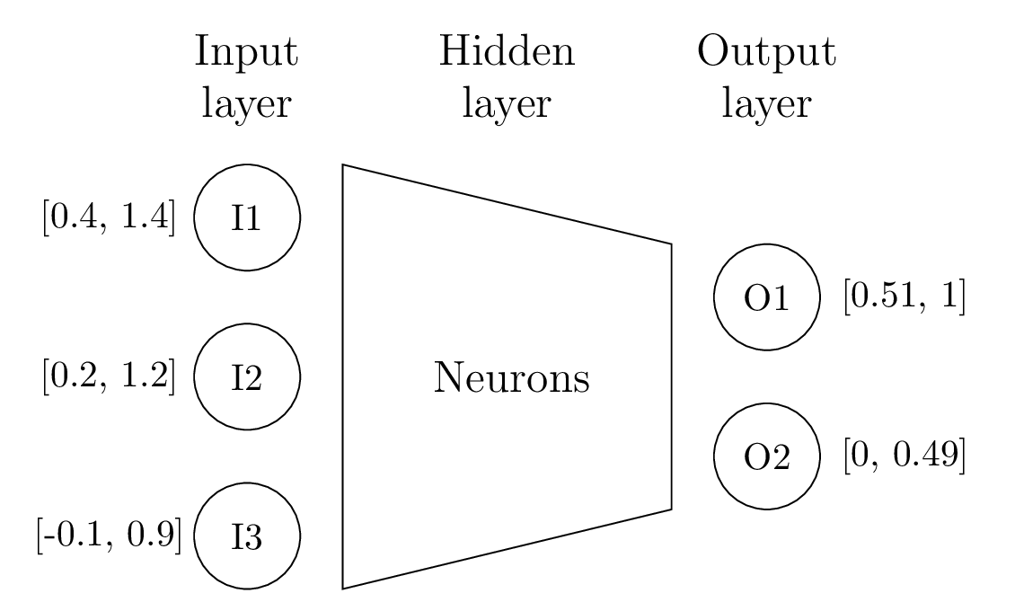
Figure 5. Robustness property example - We consider a hypercube (of size 0.5) as a neighborhood around $x=(0.9,0.7,0.4)$ and the output must always be the first class, i.e. the lower bound of the output neuron O1 must be greater than the upper bound of the neuron O2.

5. Explainability

Table 2. Summary of explanation method. The column “method name” report the technique used when the proposed method has no name

	Method name	Papers	Model targeted
Local Explanation	masking model	Dabkowski and Gal (2017)	all
	mpsm	Fong and Vedaldi (2017)	all
	lore	Guidotti et al. (2018)	all
	gve	Hendricks et al. (2016)
	influence function	Koh and Liang (2017)
	lime	Ribeiro et al. (2016)	all
	anchors	Ribeiro et al. (2018)	all
	deconvnet	Zeiler and Fergus (2014)
Global Explanation	shap	Lundberg and Lee (2017)	all
	deeplift	Shrikumar et al. (2017)
	npsem	Zhao and Hastie (2019)	all

where all = model agnostic and  = DNN specific.

As already stated earlier, explainability is a very new constraint for embedding ML-based systems. Implicitly contained in the traditionally programmed components, it has become a true challenge to demonstrate that the ML system’s outcomes are trustworthy. Improving this level of confidence seems inescapable to meet the acceptance criteria of the ML application user (designer, authorities, investigators, pilot…). It has been clearly identified as a means of acceptance in the EASA AI roadmap (EASA, 2020).

We identify two type of explanations : local explanations and global explanation. Both subdomains suit different needs: (i) explanation at the prediction level (local) and (ii) explanation of the behavior of the model regarding inputs evolution (global). In each subdomain, we face two types of explanation techniques: model agnostic and model specific. Model agnostic means that whatever the ML algorithm, we can provide an explanation (Dabkowski and Gal, 2017; Fong and Vedaldi, 2017; Guidotti et al., 2018; Lundberg and Lee, 2017; Ribeiro et al., 2016, 2018; Zhao and Hastie, 2019). Model specific means that it will only work with a specific type of ML algorithm; most papers in the literature focus on DNN (Hendricks et al., 2016; Kendall and Gal, 2017; Koh and Liang, 2017; Shrikumar et al., 2017; Zeiler and Fergus, 2014).

5.1. Local Explanation

Computer Vision is a complex domain because of the nature of the data we have to deal with: images or videos. Since the development of DNN, it has become easier to reach good performance on image classification, object detection, … However, we still do not fully understand why methods based on DNN work so well. Hence researchers develop new methods to explain, assess, and increase the confidence we can have in the decision taken by DNN for computer vision tasks.

5.1.1. Model agnostic

We will first speak of 3 systems: lime (Local Interpretable Model-agnostic Explanations) (Ribeiro et al., 2016), anchors (Ribeiro et al., 2018) and lore (LOcal Ruled-based Explanation) (Guidotti et al., 2018). Note that lore is not applicable to images. These techniques use inputs and outputs and try to approximate locally the behavior of the ML algorithm. They are based on the same principle: generate a neighborhood around a sample $x$ and provide an explanation for the sample $x$ thanks to the neighborhood. If the reader wants to go further, Garreau and von Luxburg (2020) provide theoretical explanations of lime.

The generation of the neighborhood differs according to the system. lime and anchors use an interpretable representation and apply some perturbation on it. An interpretable representation could be a binary vector where the ones are the relevant information and a perturbation could be the modification on the vector (0 switches to 1) but this should be defined according to the problem that needs to be solved. Ribeiro et al. (2016) define metrics to measure the distance between the neighbors and the original sample. anchors and lime are using the same method of neighborhood generation. lore uses a genetic algorithm to generate a balanced neighborhood. The genetic algorithm is tuned in order to create the best possible neighbors around the desired sample.

Since the neighborhood is generated, it remains to provide the explanation. In lime linear models are used while in anchors decision trees are used. For the anchors explanation, “anchors” are used, i.e. the minimum number of features that lead to the right prediction. Note that, Ribeiro et al. (2018) define several bandit algorithms in order to find the best anchors. An explanation given by lime correspond to the area of the image that help to take the decision. anchors and lore provide explanation in the IF-THEN form. Guidotti et al. (2018) (lore) extract explanations from the decision tree while Ribeiro et al. (2018) (anchors) only check the presence or absence of anchors. Figure 6 shows an example of an explanation given by lore: the $r$ corresponds to the explanation of the decision and $\Phi$ corresponds to the minimum changes that should occur to flip the decision. The original decision (0) comes from an algorithm which was trained on the German dataset to recognize good (”0”) or bad (”1”) creditor according to a set of attributes (age, sex, job, credit amount, duration, …).

- LORE r = ({credit_amount ¿ 836, housing = own, other_debtors =  none, credit_history = critical account} $\rightarrow$ decision = 0) $\Phi$ = { ({credit_amount $\leq$ 836, housing = own, other_debtors =  none, credit_history = critical account} $\rightarrow$ decision = 1), ({credit_amount ¿ 836, housing = own, other_debtors =  none, credit_history = all paid back} $\rightarrow$ decision = 1) }

Figure 6. Explanations of LORE. (taken from Guidotti et al. (2018). We only use the part of figure 9 of Guidotti et al. (2018) that concerns their method, lore.)

A popular method to explain decision on images is the saliency map (Adebayo et al., 2018; Dabkowski and Gal, 2017; Fong and Vedaldi, 2017). Intuitively, a saliency map higlights the features, i.e. the pixels on images, that the model considers to take its decision. Fong and Vedaldi (2017) propose an agnostic gradient-based method which considers explanation as meta-predictors. A meta-predictor is a rule that is used to explain the prediction of the model. One advantage of using meta-predictors as explanation is that you can measure the “faithfulness” of your explanation by computing its prediction error, i.e. it represent the number of time that the model and the rule disagree on the prediction. Then, they claim that a good explanatory rule (i.e. meta-predictor) to produce a saliency map rely on the local explanation principle. Indeed, they want to study the behavior of the model using the neighborhood of the original example. This neighborhood is given by perturbing the original example; that is why they introduce the notion of “meaningful pertubations”. They argue that the explanation would be better, if the perturbations applied to build the neighborhood of the original example mimic natural image effect. Based on meaningful perturbations, the authors define an optimization problem which tries to find the smallest area of the original image that must be perturbed in order to reduce prediction probability of the true class of the original image; This method then outputs the saliency map which give the explanation of the model’s prediction. In table 2, we named their method Meaningful Perturbation Saliency Map (mpsm).

On the other side, Dabkowski and Gal (2017) develop a masking model that learn how to generate interpretable and accurate saliency map for ML model. The authors craft a new objective function which ensures the quality of the saliency map: it ensures that the region is necessary to the good classification while its absence leads to low probability to pick the good class and at the same time it penalizes large and not smooth region. The masking model comprises features filter (input) given by a trained network and upsampler layer which upscale the input into the original image dimension in order to provide a mask. Dabkowski and Gal (2017) train the masking model by directly minimizing its new objective function; the masking model outputs saliency map with really accurate salient area (Figure 7).

(a) Input Image

(b) Generated saliency map

(c) Image multiplied by the mask

(d) Image multiplied by inverted mask

Figure 7. An example of explanations produced by Dabkowski and Gal (2017). The top row shows the explanation for the ”Egyptian cat” while the bottom row shows the explanation for the ”Beagle”. Note that produced explanations can precisely both highlight and remove the selected object from the image.

5.1.2. DNN specific

Adebayo et al. (2018) develop a methodology to test the usefulness of a saliency method for explanation. It is based on two tests: model parameter randomization test and data randomization test. A saliency method would fail the tests if it shows the same result for the randomized case and the trained case. A failure points out the independency of the saliency method regarding the architecture parameters or labeled data. With the methodology proposed by Adebayo et al. (2018), we can test model-agnostic and model-specific methods.

Few years before the works previously presented, Zeiler and Fergus (2014) introduced a method that allow to visualize the internal working of convolutional neural networks (CNN). Their motivation was to understand how and why CNN work well by studying the hidden layer of CNN. The principle is to sample the features learned by a neural network, back to the original image dimension. However, contrary to the method seen until now, the goal of the was not to provide a saliency map that explain the model’s predictions but only to visualize the feature that a neural network learned for classifying. The system develop by Zeiler and Fergus (2014) is known as multi-layered Deconvolutional Network (deconvnet). One advantage of this technique is the possibility to start from any layer in order to see at this point the features learned by the neural network.

Another way of explaining an image is literally to provide written explanations: Hendricks et al. (2016) propose a visual explanation for images. Visual explanations are defined as class discriminative and accurately described, i.e. the textual explanation highlights elements of the image which are specific to the class. The authors use VGG, a CNN for image classification, and add to it an LSTM that generates visual explanations; the efficiency of this system relies on the loss function. Precisely, Hendricks et al. (2016) define two losses for their network: one for the accurate description (relevance loss) that handles the probability of word occurrence in the sentence and the other for the class discrimination (discriminative loss) which is based on a reward function. The authors reach good results on an experiment that deals with bird classification. Figure 8, taken from the paper (Hendricks et al., 2016) shows the difference between visual explanation, image description, and class definition.

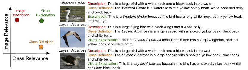
Figure 8. Visual explanations are both image relevant and class relevant. In contrast, image descriptions are image relevant, but not necessarily class relevant, and class definitions are class relevant but not necessarily image relevant. (taken from the work of Hendricks et al. (2016))

Koh and Liang (2017) through the use of influence function increase in the explanability of DNN. Unlike the other methods whose the explanability was increased by providing evidences directly on the examples, Koh and Liang (2017) to explain the prediction of an example, they provide the training datas that leads to that prediction. The principle of their method is to compute the impact on the predictions while modifying the training dataset. For explanability purpose, they study the effect of the removal of training data. The removed training data which strongly decrease the probability to get the right class of a given example are actually the data that leads to the prediction. Actually, the training data given as an explanation of a prediction provide insight on the behavior of the model. Indeed, by looking at the data that influence towards the prediction, it is possible to detect abnormal behavior of the model.

5.2. Global Explanation

As stated earlier, global explanation is the one that could explain the evolution of the model’s outputs according to the trends of the inputs. A popular method is known as “feature importance”. The principle of features importance is to find out which input features play a significant role in the decision of the ML algorithm (Lundberg and Lee, 2017; Shrikumar et al., 2017; Zhao and Hastie, 2019).

5.2.1. Model agnostic

One way of exploit the feature importance principle is to use the Shapley value which comes from cooperative game theory. The idea is to find the fair share of the gain between players in a cooperative game regarding the involvement of each player in the coalition. Lundberg and Lee (2017) develop shap (SHapley Additive exPlanations) that use the Shapley value in order to provide explanations for the predictions of ML algorithm. In this context, the features are the players and the prediction is the payout. Then, shap compute the contribution of each feature to the prediction. Since the computation of the Shapley value requires all the possible permutation of the players (features), the problem becomes intractable for inputs with numerous number of features. However, the authors provide an efficient way to compute an approximation of the Shapley value.

Zhao and Hastie (2019) study the importance of the feature through a causal model, called Non-Parametric Structural Equation Model (npsem), and using Partial Dependence Plot to visualize the results. Thanks to this approach they go further than just compute the impact of features on the prediction and manage to catch the tendency of a prediction according to the evolution of features.

5.2.2. DNN specific

Shrikumar et al. (2017) bring a new way of handling features importance with deeplift (Deep Learning Important FeaTures). The principle is to compare inputs to an input reference and outputs to an output reference. These references represent a kind of neutral behavior of the neural network. Since these references are considered as baseline, the authors backpropagate the differences between the references and the actual sample through the network by comparing the activation values. Then, they define a contribution score system that derives the features importance from the differences. Hence, at the end of the backpropagation, we end up with the importance of each feature for a given prediction. Intuitively, we would say that the greater the difference is, the more it has an impact on the feature importance. The efficiency of the algorithm depends on the choice of references that relies on domain-specific knowledge.

6. Conclusion

In this survey we have investigated the compatibility between recent advances in machine learning and established certification procedures used in civil avionic systems. Machine learning proves to be an interesting approach for developing functionalities that are difficult or impossible to implement using classical programming, such as vision-based navigation (e.g. ATTOL project from Airbus (Airbus, 2020)). This has the potential to offer meaningful improvements in the area of the system safety, and opens the way to advanced features in autonomous flight systems. However, the intrinsic characteristics of machine learning based software, such as the use of alternative requirement specification techniques or the difficult traceability of the results, seriously challenge established certification procedures.

As a first step towards certifiable embedded system based on ML, we focused on Adversarial Robustness and Explainability that will eventually support the proof of conformity to regulation requirements. With Robustness, we address the innocuity issue, inherent concept of ML algorithm inducing the necessary management of unintended behaviors of the system. With Explainability, we address the trustworthiness issue in ML algorithms which are still suffering from their black-box aspect. For both domains, our review of the state of the art shows promising methods that address those issues. It is interesting to notice that most of verification methods (cf. Section 4.2) are based on formal methods that have already been used for the demonstration of conformity since a while. Assuming that verification is the most time and cost consuming part of the development process, formal methods are promising means to handle the robustness aspects because since it provides mathematical evidences, it allows avoiding a huge amount of empirical verification. Our survey takes a closer look at some particular issues. The ultimate goal of certifying embedded systems based on ML, requires to address all the various issues identified in Figure 3 and thus demands further research in the other domains.

References

- (1)
- Adebayo et al. (2018) Julius Adebayo, Justin Gilmer, Michael Muelly, Ian J. Goodfellow, Moritz Hardt, and Been Kim. 2018. Sanity Checks for Saliency Maps. In NeurIPS.
- Airbus (2020) Airbus. 2020. Autonomous Taxi, Take-Off and Landing (ATTOL). https://www.airbus.com/newsroom/press-releases/en/2020/01/airbus-demonstrates-first-fully-automatic-visionbased-takeoff.html
- Amershi et al. (2019) Saleema Amershi, Andrew Begel, Christian Bird, Robert DeLine, Harald C. Gall, Ece Kamar, Nachiappan Nagappan, Besmira Nushi, and Thomas Zimmermann. 2019. Software Engineering for Machine Learning: A Case Study. In ICSE (SEIP), Helen Sharp and Mike Whalen (Eds.). IEEE / ACM, 291–300.
- Ashmore et al. (2019) Rob Ashmore, Radu Calinescu, and Colin Paterson. 2019. Assuring the Machine Learning Lifecycle: Desiderata, Methods, and Challenges. CoRR abs/1905.04223 (2019).
- Bahdanau et al. (2015) Dzmitry Bahdanau, Kyunghyun Cho, and Yoshua Bengio. 2015. Neural Machine Translation by Jointly Learning to Align and Translate. In ICLR.
- Baylor et al. (2017) Denis Baylor, Eric Breck, Heng-Tze Cheng, Noah Fiedel, Chuan Yu Foo, Zakaria Haque, Salem Haykal, Mustafa Ispir, Vihan Jain, Levent Koc, Chiu Yuen Koo, Lukasz Lew, Clemens Mewald, Akshay Naresh Modi, Neoklis Polyzotis, Sukriti Ramesh, Sudip Roy, Steven Euijong Whang, Martin Wicke, Jarek Wilkiewicz, Xin Zhang, and Martin Zinkevich. 2017. TFX: A TensorFlow-Based Production-Scale Machine Learning Platform. In ACM SIGKDD. ACM, 1387–1395.
- Biggio and Roli (2018) Battista Biggio and Fabio Roli. 2018. Wild Patterns: Ten Years After the Rise of Adversarial Machine Learning. Pattern Recognit. 84 (2018), 317–331.
- Cai and Zhu (2015) Li Cai and Yangyong Zhu. 2015. The Challenges of Data Quality and Data Quality Assessment in the Big Data Era. Data Science Journal 14 (2015).
- Carlini et al. (2019) Nicholas Carlini, Anish Athalye, Nicolas Papernot, Wieland Brendel, Jonas Rauber, Dimitris Tsipras, Ian J. Goodfellow, Aleksander Madry, and Alexey Kurakin. 2019. On Evaluating Adversarial Robustness. CoRR abs/1902.06705 (2019).