Influential Rank: A New Perspective of Post-training
for Robust Model against Noisy Labels

Deep neural network can easily overfit to even noisy labels due to its high capacity, which degrades the generalization performance of a model. To overcome this issue, we propose a new approach for learning from noisy labels (LNL) via post-training, which can significantly improve the generalization performance of any pre-trained model on noisy label data. To this end, we rather exploit the overfitting property of a trained model to identify mislabeled samples. Specifically, our post-training approach gradually removes samples with high influence on the decision boundary and refines the decision boundary to improve generalization performance. Our post-training approach creates great synergies when combined with the existing LNL methods. Experimental results on various real-world and synthetic benchmark datasets demonstrate the validity of our approach in diverse realistic scenarios.

1 Introduction

The current deep learning has made a huge breakthrough because of ‘data’. Thus, many researchers in both academia and industry endeavor to obtain considerable data. However, real-world data inevitably contain some proportion of incorrectly labeled data, owing to perceptual ambiguity, or errors from human or machine annotations. These noisy labels negatively affect the generalization performance of a trained model since a deep neural network (DNN) can easily overfit to even noisy labels due to its high capacity [52]. Therefore, learning from noisy labels (LNL) has received much attention in recent years [13, 49, 38, 57, 28, 5, 16] due to the increasing need to handle noisy labels in practice.

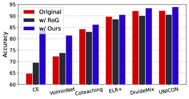
Figure 1: Test accuracy improvement over various methods on CIFAR-10N (Worst). As a post-training method, our proposed Influential Rank can improve various pre-trained models by large margin, compared to the post-processing baseline method, RoG [23]. The used CIFAR-10N (Worst) is a human-annotated real-world noisy dataset with about 40% noise rate [46].

To handle noisy-label problem, prior literature aims to distinguish between clean and mislabeled data, and use this information to train a robust classifier during training. To this end, prior works mainly rely on the assumption that the clean labels are more likely to have smaller losses before the model is overfitted [2]. However, due to the high capacity of deep neural networks (DNNs), DNNs can fit even noisy labels [52]; thus it is challenging to correctly detect mislabeled data during training. Hence, various methods have been proposed to use more robust models before overfitting, such as leveraging the model with early stopping [39, 26], or using multiple networks with co-training for sample selection [11, 51, 24].

Here, we introduce a different perspective against the mainstream research. We propose a new post-training LNL approach, which can synergize with the model trained using prior robust methods, further enhancing the generalization capability of the model. Given a pre-trained model, the proposed post-training scheme refines the model by exploiting the ‘overfitting property’ of mislabeled samples. ‘Overfitting property’ of mislabeled samples is derived from two following intuitions. (1) Mislabeled samples are more likely to distort the decision boundary than clean samples. Thus removing the mislabeled samples is likely to sway the decision boundary significantly. (2) The overfitted model predicts poorly on unseen data, and the mislabeled sample is usually the main culprit for the model to classify new data with incorrect labels. The details on these intuitions are discussed in Section 3.1.

These intuitions on overfitting motivate us to propose a novel method named Influential Rank, which leverages the samples’ influence on the decision boundary and on unseen samples to enhance robustness. To this end, we propose overfitting score on model (OSM) and overfitting score on data (OSD). OSM measures the influence of a training sample on changes in model parameters, and OSD measures the inconsistency of the sample’s influence on the classification prediction for a small number of clean validation data. Based on OSM and OSD, Influential Rank updates the trained model by removing high influential samples and mitigating their negative influence on the classifier.

Since the post-training provides a new information (i.e., sample’s influence) to any pre-trained models, Influential Rank can effectively improve robustness of existing LNL methods. Through extensive experiments on multiple benchmark data sets, we demonstrate the validity of our method, and show that Influential Rank can improve the performance of the model consistently whether or not it is pre-trained with LNL methods, as shown in Figure 1. Furthermore, we show that Influential Rank is useful in two different applications other than LNL. The proposed overfitting scores can be effective for (1) data cleansing that filters out erroneous examples in real-world video data and (2) regularization that boosts the classification performance on clean data.

Our key contributions can be summarized as follows:

• Post-training: Influential Rank is a novel post-training approach for LNL, which leverages the overfitting scores of training examples on the decision boundary.

• Practicability: Influential Rank is applicable to any pre-trained models and works synergistically with other existing LNL methods.

• Extensibility: Influential Rank can be easily extended to cleansing video dataset and a regularization for reducing overfitting arising from clean but influential samples.

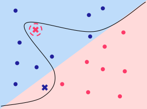
(a) Overfitted model

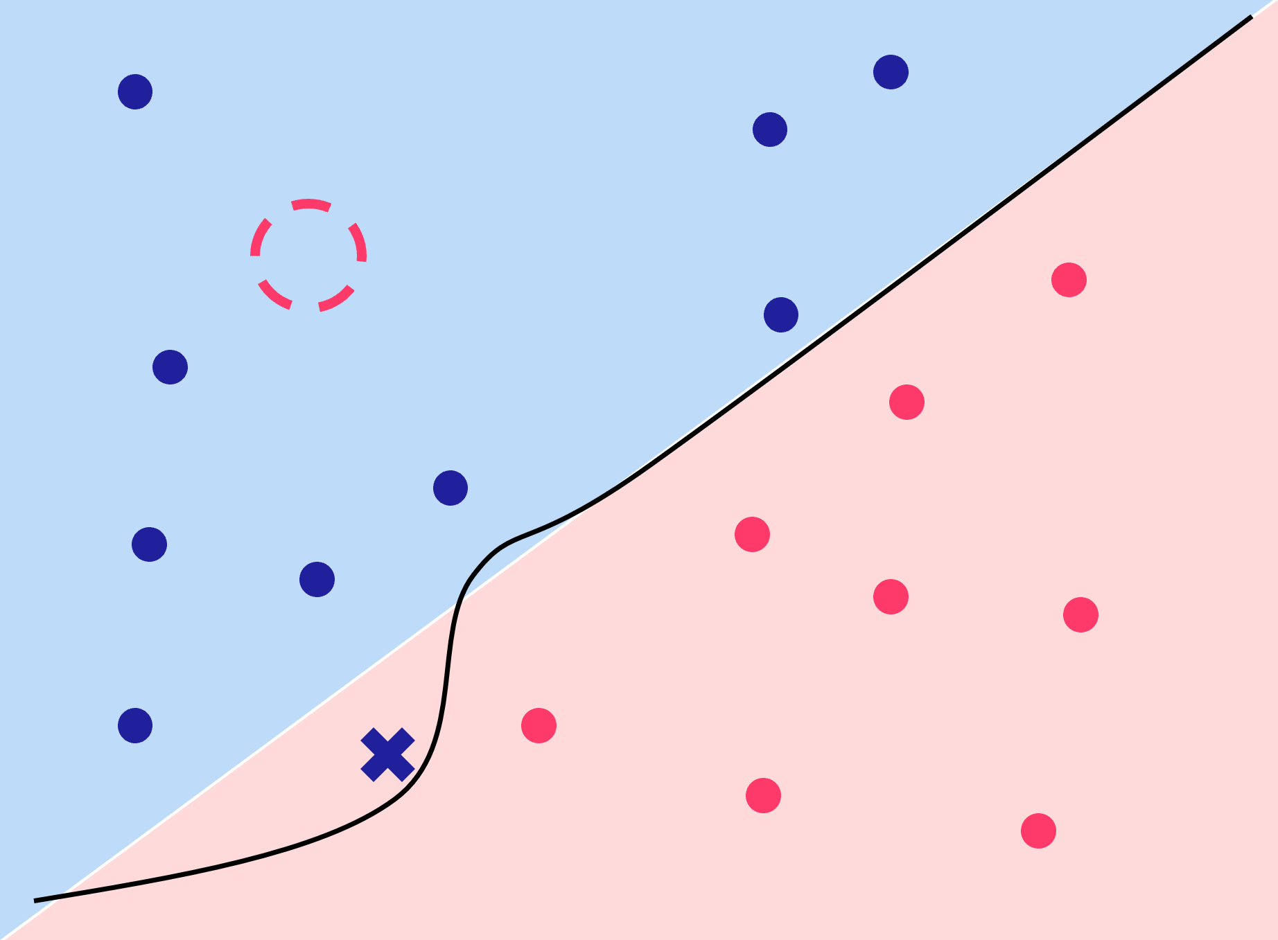
(b) Influence on model

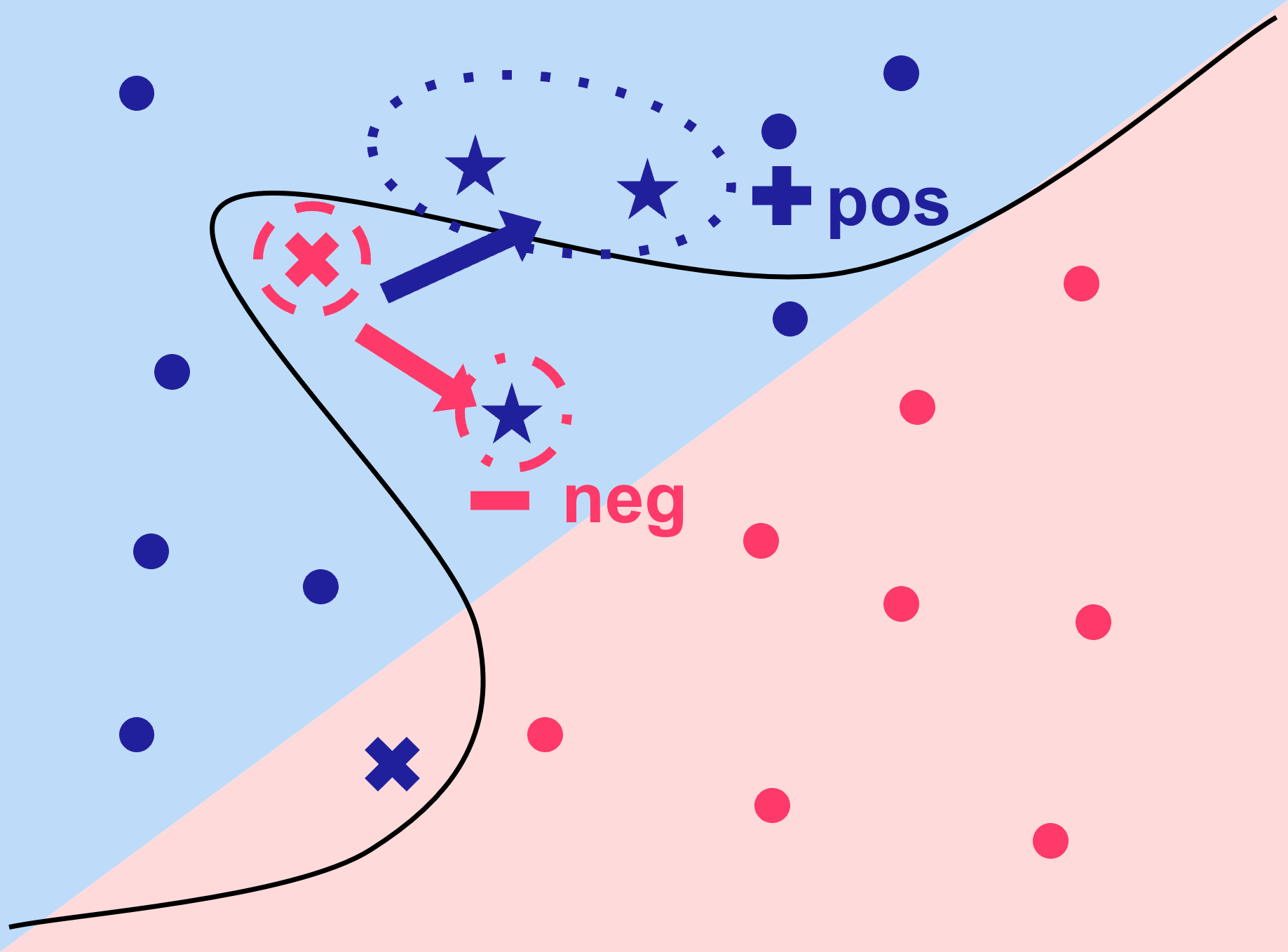
(c) Influence on data (blue)

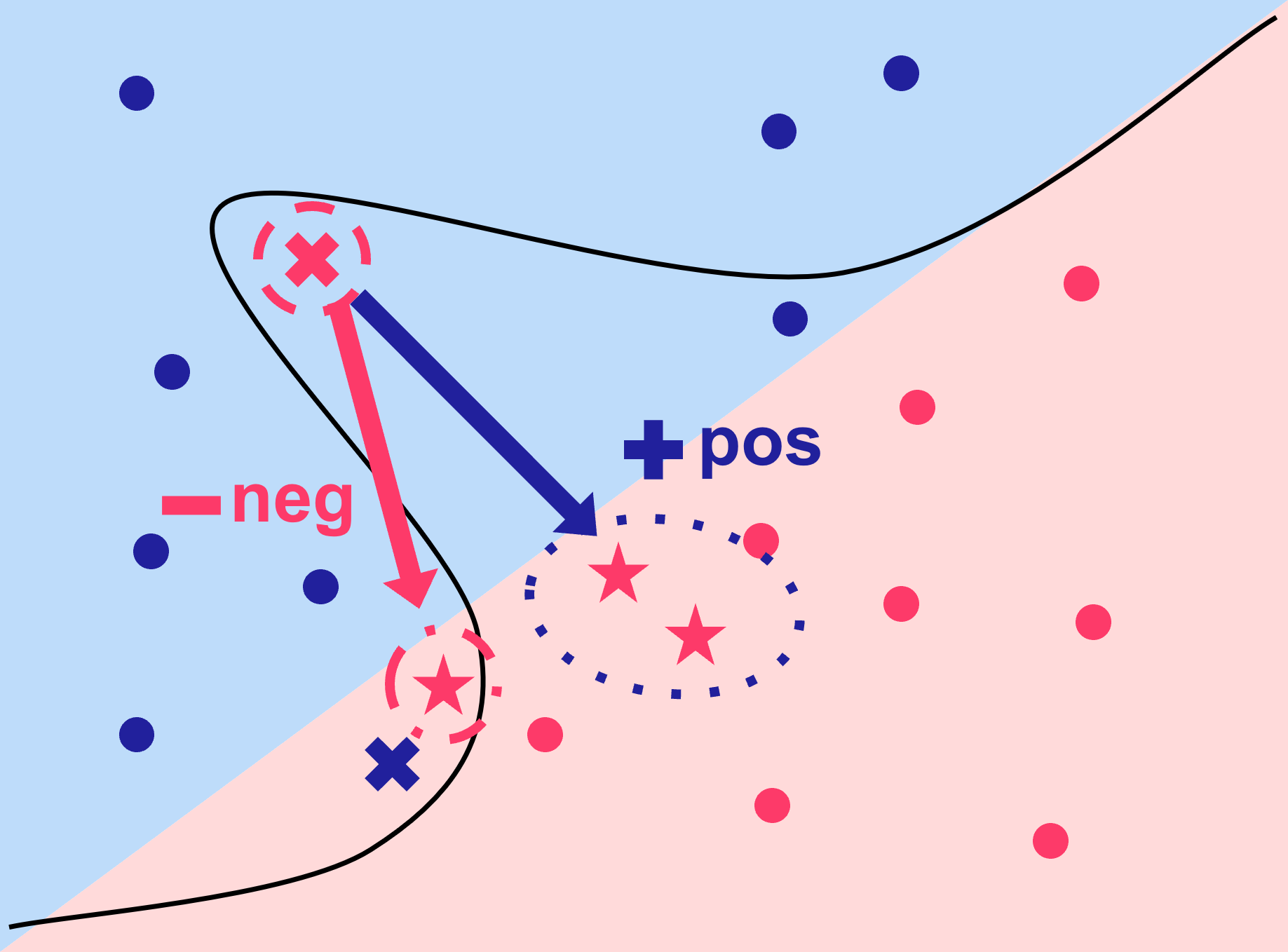
(d) Influence on data (red)

Figure 2: Our intuition. The red and blue points belong to different classes in binary classification. The $\times$ marks indicate mislabeled data. (a) Due to the mislabeled samples ($\times$), the model is overfitted. (b) $\times$ significantly affects the model because if the sample is removed, the parameter of the model is substantially changed. (c and d) Assume clean validation data ($\bigstar$) are given. The noisy-label sample ($\times$) exerts both positive and negative influences on correctly classifying the validation data in the same class, even when distances are near. The noisy-label data tend to have inconsistent effects on data within the same class.

2 Related Work

2.1 Deep Learning with Noisy Labels

Learning with noisy labels has two main research directions. One is to find and use only clean labels for training, and the other is to directly train a robust model on noisy labels. For a more thorough study on this topic, we refer the reader to survey [40, 8].

Noise-cleaning Approach. Most noise-cleaning approaches focus on finding small-loss examples before overfitting because DNNs learn easy samples first and gradually learn difficult samples [2]. To prevent overfitting of a neural network, some methods simultaneously train two neural networks and select small-loss examples [11, 51, 58, 39, 42], while others train a network guided by a teacher network [17, 56]. Meanwhile, O2U-Net [15] adjusts the learning rate to take the model from overfitting to underfitting cyclically and records the losses of each example during the iterations. DivideMix [24] and SELF [34] incorporate semi-supervised learning with the small-loss trick for better sample selection. Recently, UNICON [18] proposed uniform clean sample selection algorithm to tackle the class imbalance problem induced by prior sample selection methods.

Noise-tolerant Approach. The noise-tolerant approach aims to train a robust model on a noisy-label dataset without removing the noise. Some methods design noise-robust losses [30, 31, 55, 49, 16], and others attempt to reweight losses [33, 35]. Despite their theoretical justification, these approaches require mathematical assumptions or prior knowledge, such as known noise rates and class-conditional noise transition matrices, which make them challenging in practice. To tackle the difficulty in estimating transition matrix, Cheng et al. [5] recently proposed manifold-regularized transition matrix estimation method. Meanwhile, there are more recent efforts to add a noise adaptation layer or relabel data [9, 38, 4], but they do not perform well especially when numerous classes exist or noise rates are heavy. The main difference from existing works is that, while they follow a paradigm of ‘learning from scratch’ to prevent overfitting and regard small-loss examples as clean examples, we rather leverage the overfitting property under the ‘post-training’ paradigm, determining the most abnormal influential examples to rule out. Although RoG [23] builds a simple robust generative classifier on top of pre-trained models as post-processing, it has limited performance gain since it does not make any change to the target model and makes a strong assumption on the distribution of feature representation.

2.2 Influence Function

Finding influential examples in a dataset has been studied for decades in robust statistics [10, 6]. Recently, a few attempts have been made to apply the idea to neural networks [1, 20]. Recently, [20] used influence functions to understand the effect of a training example on a test example. Although Koh and Liang [20] showed the possibility of finding mislabels by using the influence function from email spam classification, their method requires human intervention to check and fix the examples, which is not practical. On the other hand, we propose a new criterion, overfitting scores, and a novel post-training algorithm that does not require human intervention. In addition, we extend the method to a new multimedia data, i.e., a video set, and we newly discover that the proposed method can have a regularization effect on clean data. Meanwhile, [12] proposed stochastic gradient descent (SGD) influence that can infer the influential examples for models trained with SGD. However, this method is limited to optimization by SGD and requires to store the parameters of the model at every step, requiring huge memory consumption for DNNs.

3 Influential Rank

Our idea is to leverage the property of an overfitted model for post-processing. First, we present the observations that motivated our method in Section 3.1. Then, we propose two novel criteria in Section 3.2, and we describe the overall scheme of robust post-training with overfitting scores, referred to as Influential Rank (Section 3.3). Finally, we empirically verify the effectiveness of the proposed criteria in post-training from a toy example (Section 3.4).

3.1 Intuition

Our post-training algorithm is based on two following intuitions. Mislabeled samples are likely to significantly distort the decision boundary, and to cause misclassification of nearby correctly labeled samples. Figure 2 illustrates our intuition. The red and blue points belong to different classes for binary classification, and the pink and light blue background indicates the ground-truth feature embedding space. Black line denotes a decision boundary predicted by the model. In Figure 2(a) the model overfits the mislabeld samples ( $\mathbb{\times}$ mark), thus the decision boundary is distorted compared to the ground-truth boundary. When the mislabeled sample ( $\mathbb{\times}$ mark) is removed, the trained model is substantially changed (Figure 2(b)). That is, the noisy label can exert great influence on the decision boundary of the model.

In addition, to evaluate whether a training sample causes a significantly overfitted classifier, we can use a small number of clean validation data. We consider a few validation data points (${\color[rgb]{0,0,1}\bigstar}$ marks) as shown in Figure 2(c). Because the fitted decision boundary is distorted toward the blue region to include the noisy label ( $\mathbb{\times}$ mark), the ${\color[rgb]{0,0,1}\bigstar}$ enclosed by a red dotted circle is wrongly classified into the red class. Thus, the noisy label ( $\mathbb{\times}$ mark) causes a clean sample to be misclassified (i.e., negative influence). Meanwhile, the validation samples upper the line (blue-dotted circle) are correctly classified that it can be said that the boundary created by this mislabeled sample ( $\mathbb{\times}$) has a positive influence on properly classifying other samples. Therefore, the noisy label is likely to have inconsistent influences on the clean validation samples, although their distances are near each other. The same claim can apply to the validation samples ($\bigstar$) in the other ( red) category in Figure 2(d). We verify the inconsistent influences of noisy labels in Section 4.3.3.

From this observation, we present two novel criteria that measure the abnormal influences of a training sample. One is to measure how much a training sample affects the overfitting of model parameters, referred to as the overfitting score on model, and the other measures how inconsistently a training sample affects the classification of clean validation data, which is referred to as the overfitting score on data.

3.2 Overfitting Scores

To identify overfitting on individual points for detecting noisy labels, we utilize two influence functions in  [20]. One is to measure the influence of an example $(x,y)$ on the model $f(x,\hat{\theta})$ trained on the dataset $\mathcal{D}$ via loss function $\ell(y,f(x,\theta))$, given by

$${\mathcal{I}_{M}}(x;\hat{\theta})=-H_{\hat{\theta}}^{-1}\left.\triangledown_{\theta}\ell({y},f(x,\theta))\right|_{\theta=\hat{\theta}},$$ (1)

where $H_{\hat{\theta}}\overset{\mathrm{def}}{=\joinrel=}\frac{1}{|{\mathcal{D}}|}\sum_{(x,{y})\in{\mathcal{D}}}\left.\triangledown_{\theta}^{2}\ell\big{(}{y},f(x,\theta)\big{)}\right|_{\theta=\hat{\theta}}$. The other is to measure the influence of a training sample $(x_{i},y_{i})$ on a test sample $(x_{t},y_{t})$, given by

$${\mathcal{I}_{D}}(x_{i},x_{t};\hat{\theta})=\triangledown_{\theta}\ell({y_{t}},f(x_{t},\hat{\theta}))^{\top}{\mathcal{I}_{M}}(x_{i};\hat{\theta}).\vspace{-3mm}$$ (2)

3.2.1 Overfitting Score on Model

${\cal I}_{M}(x;\hat{\theta})$ can be used to estimate the effect of a noisy label on an overfitted model (Figure 2(b)). However, ${\cal I}_{M}(x;\hat{\theta})$ is a $p$-dimensional vector, where $p$ is the number of model parameters. Thus, to measure the strength of the influence of a training point $(x_{i},y_{i})$, we use $\|{\cal I}_{M}(x_{i};\hat{\theta})\|$ as a metric. Using this metric, we define overfitting score on model (OSM) ${\mathcal{O}_{M}}(x_{i};\hat{\theta})$ as the model (parameter)’s potential change caused by ignoring the example $x_{i}$ for training,

$${\mathcal{O}_{M}}(x_{i};\hat{\theta})=\frac{\|{\mathcal{I}}_{M}(x_{i};\hat{\theta})\|-\mu_{x\in\mathcal{D}}\big{(}\|{\mathcal{I}}_{M}(x;\hat{\theta})\|\big{)}}{\sigma_{x\in\mathcal{D}}\big{(}\|{\mathcal{I}}_{M}(x;\hat{\theta})\|\big{)}},$$ (3)

where $\mu_{x\in\mathcal{D}}(\cdot)$ and $\sigma_{x\in\mathcal{D}}(\cdot)$ denote mean and standard deviation of $\|{\cal I}_{M}(x;\hat{\theta})\|$ over $x\in\mathcal{D}$, respectively.

OSM ${\mathcal{O}_{M}}(x_{i};\hat{\theta})$ measures a normalized global influence of a training sample $x_{i}$ on the entire parameters. As in Figure 2(b), the noisy samples are likely to locate near the decision boundary, therefore, they will exhibit a higher OSM than examples with clean labels.

3.2.2 Overfitting Score on Data

In contrast to a well-generalized decision boundary, an overfitted decision boundary by a mislabeled sample makes the mislabeled sample inconsistently affect clean validation samples, even though the validation samples belong to the same class (Figure 2(c) and 2(d)). Here, an influence of a training sample on a validation sample indicates how much a classification result of the validation sample changes after removing the training sample. Therefore, we suggest overfitting score on data (OSD) as the within-class influence consistency of a training sample $x_{i}$ on $m$ clean validation samples in $\mathcal{D}_{k}=\{x_{1}^{v},\cdots x_{m}^{v}\}$ in the $k$-th class. Utilizing (2), OSD ${\mathcal{O}_{D}^{k}}(x_{i};\hat{\theta})$ in the $k$-th class is defined by

$$\small{\mathcal{O}_{D}^{k}}(x_{i};\hat{\theta})=\frac{\sigma_{k}\big{(}{\cal I}_{D}\big{(}x_{i},x^{v};\hat{\theta}\big{)}\big{)}-\mu\big{(}\sigma_{k}\big{(}{\cal I}_{D}\big{(}x,x^{v};\hat{\theta}\big{)}\big{)}\big{)}}{\sigma\big{(}\sigma_{k}\big{(}{\cal I}_{D}\big{(}x,x^{v};\hat{\theta}\big{)}\big{)}\big{)}},$$ (4)

where $\sigma_{k}(\cdot)$ is standard deviation of ${\cal I}_{D}\big{(}x,x^{v};\hat{\theta}\big{)}$ over $x^{v}\in\mathcal{D}_{k}$, whereas $\mu(\cdot)$ and $\sigma(\cdot)$ denote mean and standard deviation of $\sigma_{k}(\cdot)$ over $k$.

3.3 Post-processing with Influential Rank

Algorithm 1 outlines the overall procedure of Influential Rank. Given a pre-trained model, Influential Rank updates the model parameter with the training dataset excluding highly influential examples (i.e., potentially mislabeled examples) for a fixed number of post-training epochs, which is much smaller than the total training epochs of the pre-trained model. Specifically, given a pre-trained model $\hat{\theta}_{0}$, we calculate ${\mathcal{O}_{M}}(x_{i};\hat{\theta})$ for the whole training dataset ${\mathcal{D}}$ (Line 3). Since our goal is to exclude examples that have high scores for both ${\cal O}_{M}(x_{i};\hat{\theta})$ and ${\mathcal{O}_{D}^{k}}(x_{i};\hat{\theta})$, we compute ${\mathcal{O}_{D}^{k}}(x_{i};\hat{\theta})$ for the training samples whose ${\mathcal{O}_{M}}(x_{i};\hat{\theta})$ are higher than the mean (i.e., 0) for efficient computation.

To automatically quantify the number of influential samples that need to be eliminated, we assume a two-modality Gaussian mixture model (GMM). First, we fit the two-modality GMM to ${\mathcal{O}_{D}^{k}}(x_{i};\hat{\theta})$ using the Expectation-Maximization algorithm. Next, we select the training samples whose ${\mathcal{O}_{D}^{k}}(x_{i};\hat{\theta})$ are higher than the smaller mean of the Gaussian component (Line 6). We referred to those samples as noisy candidates. Then, we decide the final influential samples if a noisy candidate is inconsistent for more than $\gamma$ classes in common (i.e., more than $\gamma$ classes have consensus that the noisy candidate is inconsistent), which are referred as noisy-probable samples (Line 8).

After removing all the noisy-probable samples, the model is retrained for a small number of epochs using the new training set (Line 9, 10). If a meaningful improvement in the classification accuracy occurs, the noisy-probable samples are eliminated from the training set, and the algorithm is repeated. Otherwise, the noisy-probable samples are not removed, and the algorithm stops.

When the algorithm finishes, new labels of the removed samples are predicted by the classifier in the last iteration. Simply, we replace the labels of the noisy data with the newly corrected labels. Then, among the corrected training data, the new clean dataset includes only the data whose softmax outputs are higher than $S$(prediction threshold). Then, the model is newly trained on the new clean dataset and is evaluated for the test dataset.

This iterative design allows to remove more mislabeled examples in an iterative manner. As the model evolves, Influential Rank can incrementally find hard-to-identify mislabeled examples that could not be detected in the previous round. Especially under the high noise-level circumstances e.g., 70% of label noise, multi-round post-training achieves significant performance gains.

Algorithm 1 Influential Rank

0:   ${\mathcal{D}}$: data, $\hat{\theta}_{0}$: pre-trained model, $epochs$: post-training epochs, $\gamma$: consensus number

0:   $\theta_{r}$: model parameter after post-training

1:  $\mathcal{C}\leftarrow{\mathcal{D}}$    /* $\mathcal{C}$ is entire clean samples in ${\mathcal{D}}$ */

2:  repeat

3:      ${\mathcal{D}_{M}}\leftarrow\{x_{i}|\{{\mathcal{O}}_{M}(x_{i};\hat{\theta}_{r})\}_{i=1}^{n}\!\geq 0\}$ // Compute Eq. (3)​​​​​​​​

4:      for class $k=1$ to $K$ do

5:          /* Compute Eq. (4) and fit GMM $(G_{low},G_{high})$ */

6:          ${\mathcal{D}_{D}^{k}}\leftarrow\{x_{i}|\{{\mathcal{O}}_{D}^{k}(x_{i};\hat{\theta}_{r})\}_{i\in{\mathcal{D}_{M}}}\geq\mu(G_{low})\}$

7:      end for

8:      $\mathcal{S}\leftarrow\{x_{i}|\sum_{k=1}^{K}1[x_{i}\in{\mathcal{D}}_{D}^{k}]\geq\gamma\}$

9:      $\mathcal{C}\leftarrow\mathcal{C}-\mathcal{S}$    /* Update the clean set */

10:      Post-train $\hat{\theta}_{r}$ on the refined clean set $\mathcal{C}$ for $epochs$

11:  until acc$(\hat{\theta}_{r})$ saturates

12:  return $\hat{\theta}_{r}$

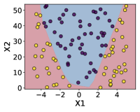
(a) Ours (Clean Model)

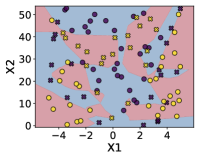
(b) Ours(Corrupted Model)

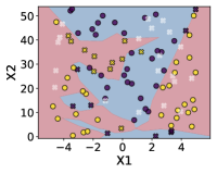
(c) OursOurs (after 1st iter.)

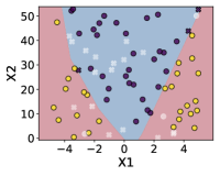
(d) OursOurs (after 3rd iter.)

Figure 3: Change in decision boundary by Influential Rank. (a) DNN trained on clean data. (b) DNN trained on noisy data (randomly chosen 40% of labels are flipped). (c) DNN after first iteration by Ours. (d) DNN after third iteration by Ours.

Table 1: Comparison on CIFAR with varying levels of symmetric label noises. The averaged test accuracy (%) with LNL methods and their combination with RoG and Influential Rank. The mean accuracy is computed over three different noise realizations.

​​Dataset​​	Method	Symm-20			Symm-50			Symm-70
		Original	+ROG [23]	​​+Inf. Rank​​	Original	+ROG [23]	​​+Inf. Rank​​	Original	+ROG [23]	​​+Inf. Rank​​
CIFAR-10	CE	80.46 (+0.0)	86.97 (+6.51)	91.08 (+10.62)	48.84 (+0.0)	62.59 (+13.76)	84.19 (+35.36)	28.42 (+0.0)	44.92 (+16.50)	70.59 (+42.17)
	VolMinNet [28]	88.26 (+0.0)	88.49 (+0.23)	91.89 (+3.63)	71.13 (+0.0)	72.65 (+1.52)	83.63 (+12.50)	33.69 (+0.0)	42.08 (+8.40)	66.07 (+32.39)
	Co-teaching [11]	91.85 (+0.0)	90.22 (-1.62)	93.10 (+1.25)	85.44 (+0.0)	81.96 (-3.48)	87.30 (+1.86)	52.63 (+0.0)	53.93 (+1.30)	60.95 (+8.33)
	ELR [29]	91.88 (+0.0)	91.50 (-0.39)	93.04 (+1.15)	88.48 (+0.0)	87.62 (-0.86)	89.60 (+1.12)	77.26 (+0.0)	72.90 (-4.36)	80.13 (+2.86)
	ELR+ [29]	93.75 (+0.0)	93.00 (-0.75)	94.73 (+0.98)	92.05 (+0.0)	91.11 (-0.94)	92.79 (+0.74)	86.94 (+0.0)	83.73 (-3.21)	88.21 (+1.27)
	DivideMix [24]	95.64 (+0.0)	95.08 (-0.56)	96.13 (+0.49)	94.02 (+0.0)	93.50 (-0.53)	94.83 (+0.80)	91.27 (+0.0)	88.69 (-2.58)	92.42 (+1.14)
	UNICON [18]	91.95 (+0.0)	91.27 (-0.68)	94.98 (+3.02)	93.59 (+0.0)	92.38 (-1.22)	95.05 (+0.09)	91.44 (+0.0)	89.38 (-2.06)	93.12 (+1.68)
CIFAR-100	CE	64.35 (+0.0)	68.21 (+3.86)	70.14 (+5.79)	39.43 (+0.0)	56.94 (+17.51)	59.31 (+19.88)	15.50 (+0.0)	39.03 (+23.53)	40.42 (+24.91)
	VolMinNet [28]	65.11 (+0.0)	64.93 (-0.18)	70.05 (+4.94)	48.77 (+0.0)	53.91 (+5.14)	58.41 (+9.64)	28.64 (+0.0)	37.02 (+8.38)	40.48 (+11.84)
	Co-teaching [11]	70.85 (+0.0)	66.93 (-3.93)	72.73 (+1.87)	59.14 (+0.0)	56.42 (-2.72)	61.29 (+2.16)	35.40 (+0.0)	35.97 (+0.57)	38.29 (+2.89)
	ELR [29]	72.58 (+0.0)	70.14 (-2.44)	74.23 (+1.66)	64.01 (+0.0)	62.91 (-1.10)	64.43 (+0.42)	38.78 (+0.0)	42.07 (+3.29)	40.07 (+1.29)
	ELR+ [29]	74.15 (+0.0)	70.29 (-3.86)	75.45 (+1.30)	65.66 (+0.0)	65.65 (-0.01)	68.74 (+3.08)	50.19 (+0.0)	54.48 (+4.29)	56.53 (+6.34)
	DivideMix [24]	76.57 (+0.0)	72.29 (-4.28)	78.63 (+2.06)	72.29 (+0.0)	68.88 (-3.41)	74.39 (+2.10)	62.43 (+0.0)	58.73 (-3.69)	65.41 (+2.98)
	UNICON [18]	74.82 (+0.0)	69.84 (-4.98)	79.61 (+4.79)	73.96 (+0.0)	68.64 (-5.32)	75.70 (+1.74)	68.61 (+0.0)	63.22 (-5.39)	69.51 (+0.90)

3.4 Example: A Binary Classification

We present a toy example to verify and visualize our hypothesis and the efficacy of the proposed overfitting scores. Figure 3 illustrates the toy example. For the two-dimensional binary classification problem, we first generate $100$ data points from the uniform distribution, where $x_{1}\sim{\rm Unif}(-5,5)$ and $x_{2}\sim{\rm Unif}(0,55)$, and their true labels $y$ are assigned following the binary rule depending on their $(x_{1},x_{2})$ values, $y=1\mbox{ if }~{}x_{2}~{}\geq~{}3x_{1}^{2}$ and $y=0\mbox{ if }~{}{\rm otherwise.}$ As can be seen in Figure 3 (c) after the first iteration excluding 20 examples with high overfitting scores and (d) after the third iteration excluding 20 more examples, the post-trained decision boundary changes into that similar to the clean model. Therefore, this toy example illustrates the validity of Influential Rank for robust post-training. The details are presented in Appendix.

4 Experiments

4.1 Experimental Settings

Datasets. We conduct classification on multiple benchmark datasets, including synthetic noisy labels and real-world noisy labels as in Table 2. A detail of datasets is presented in Appendix.

Table 2: Summary of datasets.

Dataset	# of training	noise ratio ($\varepsilon$)	noise type
CIFAR [21]	50K	20, 50, 70	synthetic
CIFAR-N [46]	40K	9, 18, 40	real-world
WebVision 1.0 [27]	2.4M	20	real-world
Clothing1M [48]	1M	38	real-world

Compared methods. We compare Influential Rank with the main baseline, RoG [23], which is the post-processing method using a robust generative classifier. We combine the two post-training methods with a default method (CE) and five state-of-the-art robust methods from different directions, i.e., a sample selection method Co-teaching [11], a robust regularization method ELR & ELR+[29], a loss correction method VolMinNet [28], a semi-supervised learning (SSL) method DivideMix [24], and a SSL & contrastive learning method, UNICON [18] . The details of the compared models and experimental settings are presented in Appendix.

Table 3: Comparison on CIFAR-N with varying levels of real-world label noise. The averaged test accuracy (%) with LNL methods and their combination with RoG and Influential Rank. The mean accuracy is computed over three different noise realizations.

CIFAR-10N

CIFAR-100N

Method

Aggregate ($\varepsilon\approx 9\%$)

Random1 ($\varepsilon\approx 18\%$)

Worst ($\varepsilon\approx 40\%$)

Noisy ($\varepsilon\approx 40\%$)

​​​​+ROG [23]​​​​

​+Inf. Rank​

​​​​+ROG [23]​​​​

​​​+Inf. Rank​​

​​​​+ROG [23]​​​​

​​​+Inf. Rank​​​

​​​​+ROG [23]​​​​

​​​+Inf. Rank​​​

CE

89.81 (+0.0)

90.19 (+0.38)

91.85 (+2.05)

83.80 (+0.0)

85.10 (+1.30)

90.05 (+6.25)

64.86 (+0.0)

69.61 (+4.76)

83.73 (+18.87)

54.71 (+0.0)

59.64 (+4.93)

62.32 (+7.61)

VolMinNet

88.59 (+0.0)

88.93 (+0.35)

91.61 (+3.02)

85.37 (+0.0)

85.94 (+0.57)

90.42 (+5.05)

72.35 (+0.0)

73.88 (+1.53)

81.51 (+9.16)

54.32 (+0.0)

56.94 (+2.62)

59.55 (+5.23 )

Coteaching

92.79 (+0.0)

91.64 (-1.16)

93.48 (+0.69)

91.59 (+0.0)

90.41 (-1.18)

92.54 (+0.95)

84.30 (+0.0)

83.10 (-1.20)

86.24 (+1.93)

61.07 (+0.0)

58.20 (-2.87)

62.75 (+1.68)

ELR

92.09 (+0.0)

91.66 (-0.43)

93.03 (+0.94)

91.59 (+0.0)

90.97 (-0.62)

92.41 (+0.82)

86.07 (+0.0)

85.48 (-0.60)

87.42 (+1.34)

62.72 (+0.0)

62.56 (-0.16)

64.65 (+1.94)

ELR+

94.36 (+0.0)

93.35 (-1.02)

94.61 (+0.24)

93.60 (+0.0)

92.53 (-1.07)

94.26 (+0.66)

89.74 (+0.0)

88.59 (-1.15)

90.54 (+0.80)

63.20 (+0.0)

63.26 (+0.06)

64.89 (+1.69)

DivideMix

94.99 (+0.0)

94.34 (-0.66)

95.46 (+0.46)

94.90 (+0.0)

94.05 (-0.84)

95.52 (+0.63)

92.24 (+0.0)

90.14 (-2.09)

93.47 (+1.23)

69.29 (+0.0)

65.39 (-3.90)

70.86 (+1.57)

UNICON

90.82 (+0.0)

90.10 (-0.72)

93.90 (+3.08)

91.87 (+0.0)

90.71 (-1.15)

94.22 (+2.35)

92.33 (+0.0)

90.61 (-1.71)

93.96 (+1.63)

68.33 (+0.0)

63.47 (-4.87)

71.04 (+2.70)

4.2 Robustness Comparison

4.2.1 Synthetic Label Noise

We conduct experiments on CIFAR dataset with different levels of symmetric noise, $\varepsilon\in\{20\%,50\%,70\%\}$. The overall classification (test) accuracies are provided in Table 1. The results show that Influential Rank consistently improves the performance of all LNL methods when combined. Also, it is noticeable that applying to a standard cross-entropy (CE) method shows the performance better than or comparable to VolMinNet. These results demonstrate that our post-processing of removing influential examples is effective under varying levels of label noise. Meanwhile, RoG shows inconsistent gains and fails to improve performance of some baselines like DivideMix and UNICON, which is attributed to the assumption of multivariate Gaussian distribution in feature representations. While we terminate the algorithm after the 2nd round, we show the results on more multiple rounds, and the noisy label detection results in Appendix.

4.2.2 Real-world Label Noise

CIFAR-10/100N. We further conduct experiment on real-world noisy CIFAR-N in Table 3. Although real-world noise is more challenging than a synthetic one, a similar trend in synthetic noisy CIFAR has been observed in real-world noisy CIFAR; the performance gain from Influential Rank is prone to increase with the increase in the noise ratio, while RoG rather decreases test accuracy in many cases.

Webvision. From Table 4, when combining Influential Rank with the state-of-the-art robust approach, DivideMix, it achieves the best performance. The top-1 accuracy of $76.24\%$ of DivideMix is further increased to $77.88\%$. In addition, it is noteworthy that our post-processing with the basic method CE shows superior performance to other complex LNL methods, such as Co-teaching and Iterative-CV.

Table 4: Comparison on WebVision with real-world label noise of $20\%$. The top-1 top-5 test accuracy. The results are taken from [24] and [29]. $\ast$ is re-trained in our experimental setup using the official code for post-training.

Method	WebVision		ILSVRC12
	Top-1	Top-5	Top-1	Top-5
MentorNet [17]	63.00	81.40	57.80	79.92
Co-teaching [11]	63.58	85.20	61.48	84.70
Iterative-CV [3]	65.24	85.34	61.60	84.98
ELR [29]	76.26	91.26	68.71	87.84
ELR+ [29]	77.78	91.68	70.29	89.76
DivideMix [24] (reported)	77.32	91.64	75.20	90.84
DivideMix [24]∗ (reproduced)	76.24	91.40	73.44	91.60
UNICON [18]	77.60	93.44	75.29	93.72
CE + Influential Rank	72.64	89.20	69.40	90.60
DivideMix∗ + Influential Rank	77.88	91.56	75.28	92.52

Table 5: Comparison with state-of-the-art methods in test accuracy(%) on Clothing1M Results for baselines are copied from original papers, and $\ast$ are reproduced by the official code.

Method	Test Accuracy
Cross-Entropy	69.21
Joint-Optim [44]	72.16
VolMinNet [28]	72.42
Meta-Cleaner [54]	72.50
ELR [29]	72.87
ELR+ [29]	74.81
Meta-Learning [25]	73.47
P-correction [50]	73.49
DivideMix (reported) [24]	74.76
DivideMix∗ (reproduced) [24]	74.23
DivideMix∗ (longer) [24]	74.42
UNICON [18]	74.98
CE + Ours	72.80
DivideMix∗ + Ours	74.90

Clothing1M. In Table 5, we compare the classification accuracy of Influential Rank with various state-of-the-art methods. Post-processing with Influential Rank to the basic training with CE loss improves the performance with a significant gap, outperforming many recent baselines. Also, applying Influential Rank to DivideMix outperforms the state-of-the-art methods. It is noteworthy that just increasing the number of training epochs cannot bring the meaningful improvement (i.e. DivideMix^∗ (longer)). While UNICON shows the superior performance, they train much longer hours with 350 epochs. Also, we believe that further performance improvement can be obtained if Influential Rank is applied for multiple rounds.

4.3 Empirical Analysis

4.3.1 Comparison with Small-loss Removal

In this section, we show that Influential Rank can be more effective for post-training the pre-trained model than using ‘small loss’ tricks, which existing methods rely on.

First, we quantitatively show our overfitting scores are superior to the small-loss trick for post-training. Specifically, the loss of each example is used instead of the overfitting scores in Eqs. (3) and (4) for removing mislabeled examples. Hence, we design a modified version we call ‘CE + Small-loss’, which excludes high-loss examples following our proposed post-training pipeline. Table 6 compares Influential Rank with the modified version of robust post-training on CIFAR-10 with synthetic and real-world label noise. It is observed that the Influential Rank provides a much larger improvement compared to loss-based removal.

Next, Figure 4 compares the distribution of the normalized loss and OSM of training samples on the pretrained model with DivideMix. Since training losses are distributed close to 0, it is difficult to classify clean and mislabeled samples with losses after training is done. However, we argue that OSM can provide a new perspective to identify ‘confusing’ examples with incorrect labels.

Table 6: Comparison with post-training using the small-loss trick on CIFAR-10 with synthetic and real-world noise. We report the best test accuracy (%).

Method	​CIFAR-10 (Symm-70)	CIFAR-10N (Worst)
CE	29.91	63.94
CE + Small-loss	53.43	76.16
CE + Inf. Rank	75.98	84.27

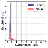
(a) Training Loss.

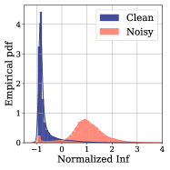
(b) OSM.

Figure 4: Loss and OSM distribution for all noisy training examples after training CIFAR-10 with symmetric noise of $40\%$.

Table 7: Mean test accuracy of training with longer epochs (‘+ Longer’) on CIFAR-10 with synthetic and real-world label noise.

	CIFAR-10 (Symm-70)			CIFAR-10N (Worst)
	Original	+Longer	+Inf.Rank	Original	+Longer	+Inf.Rank
CE	28.42	29.60	70.59	64.86	66.92	83.73
VolMinNet [28]	33.69	35.09	66.07	72.35	72.81	81.51
Coteaching [11]	52.63	53.51	60.95	84.30	84.83	86.24
ELR [29]	77.26	77.83	80.13	86.07	86.18	87.42
ELR+ [29]	86.94	87.59	88.21	89.74	00.00	90.54
DivideMix [24]	91.27	92.00	92.42	92.24	92.46	93.47
UNICON [18]	91.44	92.28	93.12	92.33	93.18	93.96

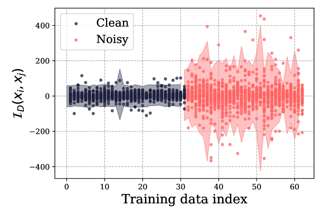
Figure 5: OSD distribution of training samples on validation samples. Shaded areas show the variance of ${\cal I}_{D}$s of each training sample. The difference in variance between the clean and noisy sets is clearly distinguished.

(a) Mislabeled as ‘Swing baseball’.

(b) Mislabeled as ‘Jump’.

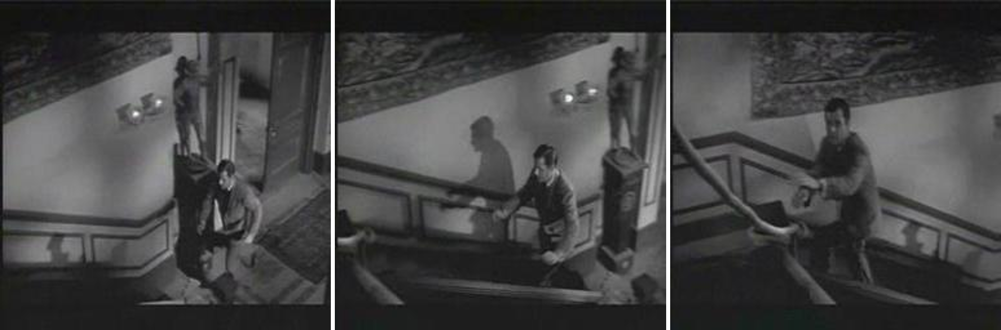
(c) Mislabeled as ‘Run’.

Figure 6: Examples with high OSM of training data. In the video clips, the labeled actions did not appear. Surprisingly, a considerable number of video clips with incorrect labels are detected, which can be found in Appendix.

4.3.2 Training with Longer Epochs

It is of interest to see whether or not the performance improvement comes from additional training epochs used for post-training, though it is reasonably shorter than the total number of epochs used for pre-training. Table 7 shows the performance of the existing state-of-the-art robust methods when training the model with longer epochs, where the number of post-training epochs (i.e., 40) is added to the original epochs (see the columns marked with ‘+Longer’). In general, the performance of the robust methods remains similarly even with longer training epochs. Therefore, our post-training approach is more desirable than simply increasing the training epochs.

4.3.3 Validity of OSD.

To show the validity of OSD, we investigate the distribution of the ${\mathcal{I}_{D}}(x_{i},x_{t}^{v};\hat{\theta})$ on real-world images. We use 1,000 ‘dog’ and ‘fish’ images from ImageNet [36], where 20% labels are randomly flipped. After training the model on this noisy dataset, we calculate OSD using 80 clean validation samples. The OSD distribution is illustrated in Figure 5 The horizontal axis is the index of the training data, and the vertical axis is OSD of a training sample $x_{i}$ on a validation sample $x_{t}^{v}$, i.e., ${\mathcal{I}_{D}}(x_{i},x_{t}^{v};\hat{\theta})$. We measure OSD on 40 validation samples for each training sample. As illustrated in Figure 5, the variation of the influence of a noisy training sample is much larger than a clean training sample. It verifies our intuition that the mislabeled samples exert much more inconsistent influences on validation data than the clean samples do. Therefore, the variance of influences, $\sigma_{k}({\cal I}_{D}(x_{i},x^{v};\hat{\theta}))$ in Eq. (4) can be used to find the mislabeled samples. This distribution appears consistently in other categories. In addition, we show that clean and noisy labels can be detected by fitting GMM model on OSD in Appendix.

4.3.4 Effects of hyperparameter.

To analyze the effects of the hyperparameter $\gamma$, we experiment with different values of $\gamma$ on CIFAR-10 trained with DivideMix. The higher gamma leads to the higher precision, but less data is erased. Therefore, choosing $\gamma$ is a tradeoff between the more accurate detection and the faster cleansing. The details are included in Appendix.

4.4 Detector for Video Data Cleaning

In this section, we show that the proposed overfitting score can be expanded to detecting mislabeled videos. Data cleaning for real-world video data is gaining significant attention due to the growth in the popularity of video-based tasks [19, 32, 47]. However, detecting video clips with incorrect labels are time-consuming for human annotators more than exploring images because it requires to play and watch the video clip one by one; thus, automatic cleaning of video data can help reduce extreme labeling costs. Therefore, we extend our work to video action recognition for data cleaning.

We first train the TSN architecture [45] on HMDB-51 data [22] for action recognition. Since each video clip has multiple scenes, the overfitting score of the clip is computed by averaging the score for randomly sampled scenes in the clip. Then, we filter out mislabeled video clips based on the proposed OSD. Figure 6 shows some examples of detected mislabeled video clips by Influential Rank. While HMDB-51 has been known to be clean, surprisingly, we observe that some videos are incorrectly labeled and do not contain any scene corresponding to the label. We include more detected examples and details of implementation in Appendix.

4.5 Regularizer for Performance Boosting

As another use case, Influential Rank can be considered as a regularizer to avoid overfitting, when there is no apparent label noise in training data. Recently, many regularization techniques have been proposed to reduce the generalization gap of DNNs [41, 53]. Our method post-processes the overfitted decision boundary by squeezing out the negative impact of highly influential examples. Thus, it has the potential to be used as regularization to smooth decision boundaries.

As a case study, we conduct an experiment on clean CIFAR-10 using the same experimental configuration. Table 8 and Figure 7 shows that Influential Rank can also improve the model trained on clean dataset. We conjecture that this is because Influential Rank removes spurious or isolated data points leading the decision boundary astray, and get a well-generalized decision boundary.

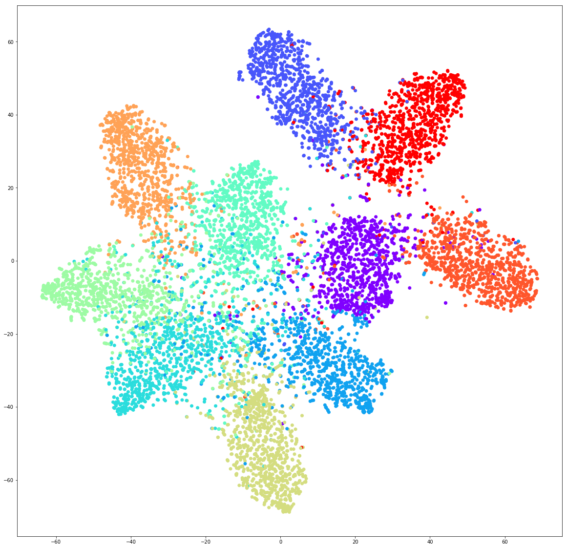
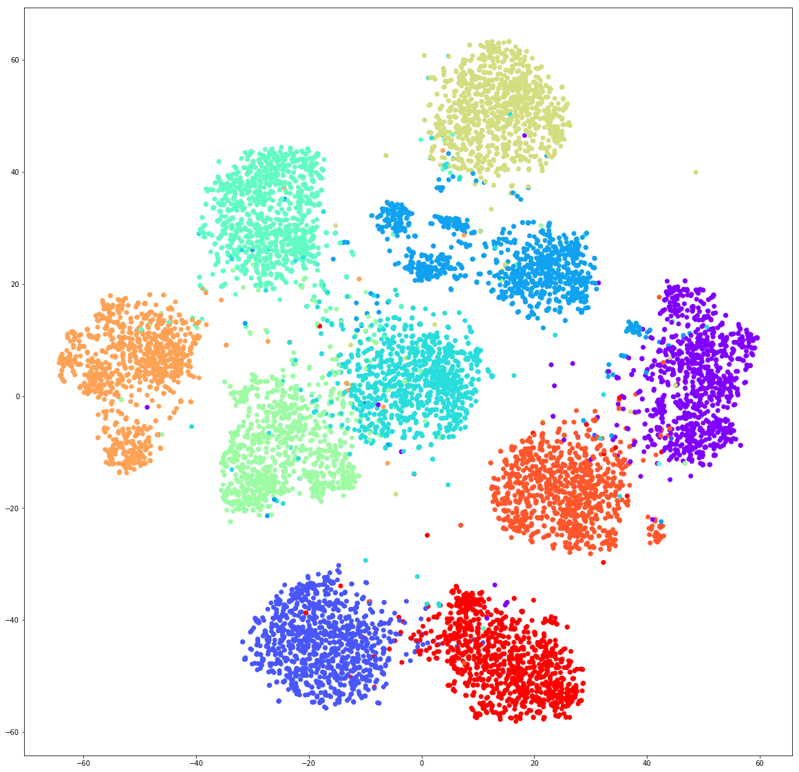
(a) W. Influential Rank.

Figure 7: t-SNE visualization for the learned representation of the trained models.

Table 8: Result of Influential Rank on clean CIFAR-10.

	# of training	Accuracy
Original	50,000	94.2
+Inf. Rank	48,989	96.6

5 Conclusion

We have proposed a post-training method named Influential Rank, which sways the overfitted decision boundary to be correct, in the presence of noisy labels. Unlike the existing methods, Influential Rank starts from an overfitted model and makes the model more robust against noisy labels progressively. We have conducted extensive experiments on real-world and synthetic noisy benchmark datasets. The results demonstrate that Influential Rank consistently provides performance gain when combined with multiple state-of-the-art robust learning methods. In addition, we have shown that Influential Rank performs as a detector for video data cleaning or a regularizer to smooth the decision boundary.

Supplementary Material

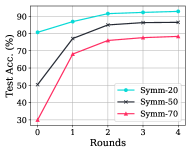
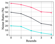
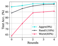
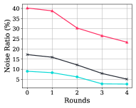
(a) CIFAR-10 with Synthetic Noise.                               (b) CIFAR-10N with Real-world Noise.

Figure 8: Effect of multi-round post-training on CIFAR-10 with synthetic label noise and real-world. (Left: Test accuracy over rounds by Influential Rank over rounds, Right: Noise ratio of the refined data.)

Appendix A Example of Influential Rank: A Binary Classification

In Figure 3, yellow and purple circles represent examples of two different classes, and blue and pink shades indicate their decision surfaces. Next, for the label noise scenario, $40\%$ of the true labels are randomly corrupted in data, i.e., $\times$ marks in Figure  3(b). Then, we fit a two-layer feedforward neural network with 50 hidden neurons.

Figure  3(a) shows that the decision boundary trained on clean data is well-formed close to the ground truth. However, when trained with noisy labels shown in Figure  3(b), we observe that the trained model overfits to mislabeled examples, and forms a complex decision boundary such that many mislabeled examples locate near the overfitted decision boundary. When we post-train the model after excluding 20 examples with high overfitting scores (i.e., white examples), the overfitted decision boundary begins to recover in Figure 3(c). Again, after excluding total 20 more high influential examples after the third iteration in Figure 3(d), the decision boundary becomes almost similar to that of the clean model. Therefore, this toy example justifies our proposed Influential Rank.

Appendix B Experimental Setting

B.1 Datasets

For CIFAR-10 and CIFAR-100, noisy labels are injected using the symmetric noise [11] of flipping true labels into other labels with equal probability $\varepsilon$, i.e., the noise ratio. Regarding the real-world noisy data, CIFAR-N [46] has various versions of human noise level. ‘aggregate’ ($9\%)$, ‘random’ ($18\%)$, and ‘worst’ ($40\%)$, while CIFAR-100N has only a single version, ‘noisy’ ($40\%$). Clothing1M includes about $38\%$ real noisy labels, and WebVision 1.0 contains about $20\%$ real-world noisy labels [40]. Following the previous work [3], we only use the first 50 classes of the Google image subset in WebVision. Lastly, we use a video stream data, HMDB-51 [37], to verify that our method can be effective as a detector for data cleaning.

To illustrate the applicability of our algorithm to video streams, we experiment on HMDB-51, a popular dataset frequently used in video action recognition [37]. Clothing1M and WebVision 1.0 are large-scale real-world datasets. Clothing1M includes about $38\%$ real noisy labels and WebVision 1.0 contains about $20\%$ noisy labels. Following previous work [3], we compare baseline methods on the first 50 classes of the Google image subset. Furthermore, to illustrate the applicability of our algorithm to video streams, we experiment on HMDB-51, a popular dataset frequently used in video action recognition [37].

B.2 Implementation Details

In this section, we describe more implementation details which are not included in Section  4.1. Following the prior literature [29], all the compared methods are trained using ResNet-34, Inception-ResNet V2, and ResNet-50 for CIFAR, WebVision datasets, and Clothing1M respectively. For all experiments, the last fully connected (FC) layers in the networks are used as the overfitted classifiers. In addition, to reduce the number of the classifier parameters, we add a penultimate FC layer with 50, 100, 100 neurons, for CIFAR-100, WebVision 1.0, and HMDB-51, respectively. This allows to save the computational cost of hessian computation. Lastly, for label refinement, we set the threshold $S$ to 0.8. We will make our code publicly available after publication.

B.2.1 CIFAR and CIFAR-N

All networks are trained for 120 epochs for CIFAR-10(N), and 150 epochs for CIFAR-100(N) with Stochastic Gradient Descent (SGD) (momentum=0.9). Regarding to training with CE, we set the initial learning rate as 0.1, and reduce it by a factor of 10 after 40 and 80 epochs for CIFAR-10(N). For CIFAR-100(N), the initial learning rate is decayed at 60th and 100th epoch by 0.1. To implement LNL baselines, we set the hyperparameters and training scheme for the baselines as reported in their original papers [11, 29, 24, 28]. In all experiments, we use the standard data augmentation of horizontal random flipping and 32 × 32 random cropping after padding 4 pixels around images. Following the recent works, we also adopt the augmentation policy from [7].

For the results in Table  1 and  3, the algorithm is applied for 2 rounds with 20 epochs each. For post-training iteration, we set the initial learning rate as same as the one used in earlier pre-training, and drop it after 5 epochs. For cross-entropy (CE) loss, the learning rate at start is set to 0.1 and is decreased by a factor of 0.1 after the 5th and 15th epoch. By increasing the learning rate high at the first epoch in each retraining iteration, we can encourage the network to explore a newly updated dataset and form a new classifier. We apply RoG and Influential Rank to the models from the last epoch. Influential Rank and RoG both use 500 validation samples. Experiments are conducted with three different noise realizations and the averaged test accuracies are reported.

B.2.2 WebVision

For WebVision 1.0, we use inception-resnet v2 [43] following [3]. For fair comparison with other baselines, both networks are trained for 80 epochs first, and then post-trained with Influential Rank for 20 epochs. We train the network with CE loss for 80 epochs using the SGD optimizer (momentum=0.9) with an initial learning rate 0.01, which is divided by 10 after 50 epochs. When training with DivideMix [24], we follow the setting in their original paper. After 1 round of Influential Rank, 5K and 6K highly influential examples are removed in CE and DivideMix, respectively. When post-training, both networks are trained for 20 epochs with a learning rate 0.01, and the learning rate is dropped to 0.01 after 10 epochs.

B.2.3 Clothing1M

For Clothing1M, the network is initially trained for 80 epochs with learning rate $0.002$ which is decreased by a factor of 0.1 after 40 epochs. We set a batch size to 64, and train the network using SGD optimizer (momentum=0.9) with CE. When training with DivideMix [24], we follow the setting in their original paper. After 1 round of Influential Rank, 140K and 230K highly influential examples are removed in CE and DivideMix, respectively. For post-training with CE, the model is trained with a learning rate of 0.002 for 10 epochs and then the learning rate is dropped to 0.0002. For post-training with DivideMix, the model is trained with a learning rate of 0.0002 for 10 epochs and then the learning rate is dropped to 0.00002.

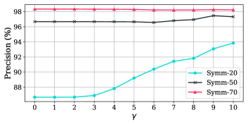
(a) Precision.

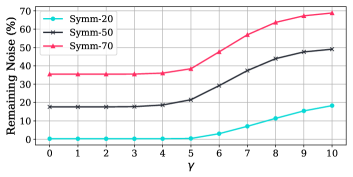
(b) Remaining Noise.

Figure 9: Effects of $\gamma$. Influential Rank is applied to the model trained on CIFAR-10 with DivideMix.

B.3 Calculation of Hessian

We calculate the Hessian matrix using only sampled $n$ ($\ll N$) data to reduce the computation cost, which is a reasonable approximation by the law of large numbers when the volume of training data is large. For deep neural networks (DNNs), the Hessian matrix could not be positive definite, so we added a positive constant 0.01 to the diagonal following [20]. To efficiently calculate the inverse of the Hessian matrix, we also adopt the conjugate gradient method from optimization theory. The conjugate methods do not require explicitly computing the inverse of the hessian, thus computational complexity is only $O(np)$, where $p$ is the number of parameters of the last fully connected layer. In most cases, we simply use open library to calculate the inverse of the Hessian because the number of parameters is sufficiently reduced and many open libraries, (e.g., NumPy), provide optimized solutions.

Appendix C Further Analysis

C.1 Effects of Multi-round Post-training

To verify the potential benefit of using multi-round post-training, we set the number of total rounds to $4$, and post-train the network, which is pre-trained using the plain CE. Figure 8 depicts the effect of the multi-round post-training on CIFAR-10 and CIFAR-10N, where the round $0$ means the model before any post-training. Overall, the noise ratio of the refined data by Influential Rank reduces gradually as the round goes up. In CIFAR-10 of Figure 8(a), the test accuracy is largely improved to 92.83%, 86.49%, and 78.34% from the initial accuracy of 80.71%, 50.37%, 29.91%, respectively. In addition, the initial noise ratios of 20%, 50%, and 70% become 1.12%, 21.43%, and 48.81% at the final round of post-training. Consistently, this improvement trend is exactly the same in CIFAR-10N with real-world noise in Figure 8(b). Particularly, the improvement in noise ratio and test error becomes larger when data is corrupted with heavier noise. While performance increase can be expected with multi-rounds, we discover that setting only 2-3 rounds can be sufficiently beneficial in terms of increasing computational burdens.

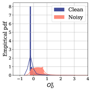
(a) CE

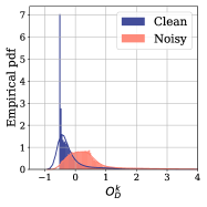
(b) DivideMix

Figure 10: OSD distribution for all noisy training examples after training CIFAR-10 with symmetric noise of $50\%$.

C.2 Effects of hyperparameter

Choosing a high $\gamma$ increases the precision of the detected noisy label since it means that a training point exerts inconsistent influences to many classes (Figure 9). On the other hand, to meet the high standard (e.g., unanimous consensus among all classes), it cannot but select less noisy samples, which results in the ratio of the remaining noisy labels to be high. Therefore, choosing $\gamma$ is a tradeoff between the more accurate detection and the faster cleansing. Therefore, in our experiments, the gamma is set to 5 in order to fix the data faster when the noise ratio is more than 40%, and set to 8 in the other cases.

Furthermore, setting $\gamma=0$ is equivalent to using only OSM in the algorithm. Hence, it is verified that OSD helps to increase the precision of noisy label detection.

C.3 Distribution of OSD

To find noisy candidates, we fit a two-modality Gaussian mixture model (GMM) to ${\mathcal{O}_{D}^{k}}(x_{i};\hat{\theta})$ for $k$-th class. To justify if GMM can detect noisy candidates, we plot the distribution of training samples’ ${\mathcal{O}_{D}^{k}}(x_{i};\hat{\theta})$ (i.e., 6th class) in Figure 10. We calculate OSD from two models trained on CIFAR-10 (Symm-50) with CE and DivideMix, respectively. As shown in Figure 10, OSD of clean and noisy samples is bi-modal and separable. Thus, we fit the two-modality GMM into the OSD of all training examples to choose noisy candidates in the proposed algorithm. This observation is consistent even when the model is trained with the existing robust methods.

C.4 Noisy Label Detection with Influential Rank

We report the noise ratio change after applying Influential Rank (2 rounds) on CIFAR and CIFAR-N in Table 9. As can be seen from the tables, the original noise ratio has been largely alleviated after applying Influential Rank. As can be seen from Section  C.1, applying Influential Rank for more rounds can further alleviate the noise ratio in datasets.

Furthermore, we present the noisy label detection precision in Table 10. We can observe that mislabeled samples are detected with high precision on both symmetric and real-world noisy data.

Table 9: Averaged noise ratio (%) after Influential Rank (2 rounds).

(a) CIFAR with symmetric noise.                                                   (b) CIFAR-N.

	CIFAR-10			CIFAR-100
	Symm-20	Symm-50	Symm-70	Symm-20	Symm-50	Symm-70
No Post-processing	20	50	70	20	50	70
CE	8.83	37.01	62.71	12.15	45.11	64.67
VolMinNet [28]	4.42	36.68	61.02	5.53	31.46	55.15
Co-teaching [11]	3.99	35.26	64.95	6.63	31.81	59.40
ELR [29]	5.51	39.99	63.73	6.52	30.34	60.48
DivideMix [24]	3.84	22.79	42.11	7.18	26.53	49.81
UNICON [18]	4.34	29.36	54.72	5.26	30.43	55.31

	CIFAR-10N			CIFAR-100N
	Aggregate	Random1	Worst	Noisy
No Post-processing	9	18	40	40
CE	5.30	11.07	29.79	34.20
VolMinNet [28]	2.48	4.54	38.61	31.24
Co-teaching [11]	2.32	4.33	26.55	28.56
ELR [29]	1.05	3.26	26.51	27.67
DivideMix [24]	1.11	2.98	18.32	27.28
UNICON [18]	1.55	6.52	23.63	25.23

Table 10: Averaged precision (%) of noise detection after Influential Rank (2 rounds).

(a) CIFAR with symmetric noise.                                                   (b) CIFAR-N.

	CIFAR-10			CIFAR-100
	Symm-20	Symm-50	Symm-70	Symm-20	Symm-50	Symm-70
CE	82.84	92.23	93.36	62.38	73.35	86.34
VolMinNet [28]	91.56	99.79	94.01	94.80	98.63	97.13
Co-teaching [11]	96.41	99.90	88.82	94.37	98.52	92.42
ELR [29]	96.37	99.55	99.58	83.14	92.48	92.76
DivideMix [24]	93.91	96.97	98.69	74.56	91.95	96.06
UNICON [18]	86.88	97.96	99.44	85.35	97.47	97.64

	CIFAR-10N			CIFAR-100N
	Aggregate	Random1	Worst	Noisy
CE	59.48	85.07	90.19	74.32
VolMinNet [28]	61.35	74.33	98.96	89.38
Co-teaching [11]	64.46	88.49	98.89	89.71
ELR [29]	65.31	91.48	98.92	89.29
DivideMix [24]	70.19	90.68	95.51	86.55
UNICON [18]	54.77	80.11	96.51	85.54

Table 11: Comparison on CIFAR with varying levels of label noises (1 round). The averaged test accuracy (%) with LNL methods and their combination with Influential Rank. The mean accuracy is computed over three different noise realizations.

Method

CIFAR-10

CIFAR-100

Symm-20

Symm-50

Symm-70

Symm-20

Symm-50

Symm-70

Original

+Inf. Rank

Original

+Inf. Rank

Original

+Inf. Rank

Original

+Inf. Rank

Original

+Inf. Rank

Original

+Inf. Rank

CE

80.46 (+0.0)

87.46 (+7.00)

48.84 (+0.0)

78.14 (+29.31)

28.42 (+0.0)

65.33 (+36.91)

64.35 (+0.0)

67.20 (+2.85)

39.43 (+0.0)

47.36 (+7.93)

15.50 (+0.0)

25.26 (+9.76)

VolMinNet [28]

88.26 (+0.0)

90.90 (+2.64)

71.13 (+0.0)

82.05 (+10.92)

33.69 (+0.0)

63.50 (+29.82)

65.11 (+0.0)

68.48 (+3.37)

48.77 (+0.0)

56.15 (+7.38)

28.64 (+0.0)

36.86 (+8.22)

Co-teaching [11]

91.85 (+0.0)

92.77 (+0.92)

85.44 (+0.0)

87.04 (+1.61)

52.63 (+0.0)

56.92 (+4.30)

70.85 (+0.0)

71.42 (+0.56)

59.14 (+0.0)

61.01 (+1.87)

35.78 (+0.0)

37.56 (+2.16)

ELR [29]

91.88 (+0.0)

92.52 (+0.64)

88.48 (+0.0)

89.13 (+0.65)

77.26 (+0.0)

79.20 (+1.94)

72.58 (+0.0)

73.41 (+0.83)

64.01 (+0.0)

64.36 (+0.36)

38.78 (+0.0)

38.89 (+0.11)

ELR+ [29]

93.75 (+0.0)

94.07 (+0.32)

92.05 (+0.0)

92.40 (+0.35)

86.94 (+0.0)

87.56 (+0.62)

74.15 (+0.0)

74.93 (+0.78)

65.66 (+0.0)

68.52 (+2.86)

50.19 (+0.0)

52.55 (+2.36)

DivideMix [24]

95.64 (+0.0)

95.96 (+0.32)

94.02 (+0.0)

94.61 (+0.59)

91.27 (+0.0)

93.28 (+2.01)

76.57 (+0.0)

77.83 (+1.25)

72.29 (+0.0)

73.49 (+1.20)

62.43 (+0.0)

64.43 (+2.00)

UNICON [18]

91.95 (+0.0)

94.52 (+2.56)

93.59 (+0.0)

94.75 (+1.16)

91.44 (+0.0)

92.84 (+1.40)

74.82 (+0.0)

79.22 (+4.40)

73.96 (+0.0)

75.36 (+1.40)

68.61 (+0.0)

69.63 (+1.02)

Table 12: Comparison on CIFAR-N with varying levels of real-world noises (1 round). The averaged test accuracy (%) with robust methods and their combination with RoG and Influential Rank. The mean accuracy is computed over three different noise realizations.

Method	CIFAR-10N						CIFAR-100N
	Aggre		Rand1		Worst		Noisy
	Original	+Inf. Rank	Original	+Inf. Rank	Original	+Inf. Rank	Original	+Inf. Rank
CE	89.81 (+0.0)	90.79 (+0.98)	83.80 (+0.0)	87.98 (+4.18)	64.86 (+0.0)	78.56 (+13.70)	54.71 (+0.0)	59.77 (+5.06)
VolMinNet [28]	88.59 (+0.0)	90.72 (+2.14)	85.37 (+0.0)	88.95 (+3.58)	72.35 (+0.0)	78.97 (+6.63)	54.32 (+0.0)	56.94 (+4.36)
Co-teaching [11]	92.79 (+0.0)	93.28 (+0.49)	91.59 (+0.0)	92.13 (+0.54)	84.30 (+0.0)	86.03 (+1.72)	61.07 (+0.0)	62.36 (+1.29)
ELR [29]	92.09 (+0.0)	92.78 (+0.69)	91.59 (+0.0)	92.09 (+0.50)	86.07 (+0.0)	87.21 (+1.14)	62.72 (+0.0)	64.02 (+1.31)
ELR+ [29]	94.36 (+0.0)	94.40 (+0.04)	93.60 (+0.0)	93.85 (+0.25)	89.74 (+0.0)	90.39 (+0.65)	63.20 (+0.0)	64.28 (+1.07)
DivideMix [24]	94.99 (+0.0)	95.35 (+0.35)	94.90 (+0.0)	95.37 (+0.47)	92.24 (+0.0)	93.24 (+1.00)	69.29 (+0.0)	70.67 (+1.38)
UNICON [18]	90.82 (+0.0)	93.49 (+2.67)	91.87 (+0.0)	93.96 (+2.09)	92.33 (+0.0)	93.79 (+1.46)	68.33 (+0.0)	70.68 (+2.35)

(a) labeled as ‘Jump’.

(b) labeled as ‘Dive’.

(c) labeled as ‘Hit’.

(d) labeled as ‘Dive’. (Jump?)

(e) labeled as ‘Punch’. (Kick?)

(f) labeled as ‘Punch’. (Hit? Sword?)

(g) labeled as ‘Kick’. (Run?)

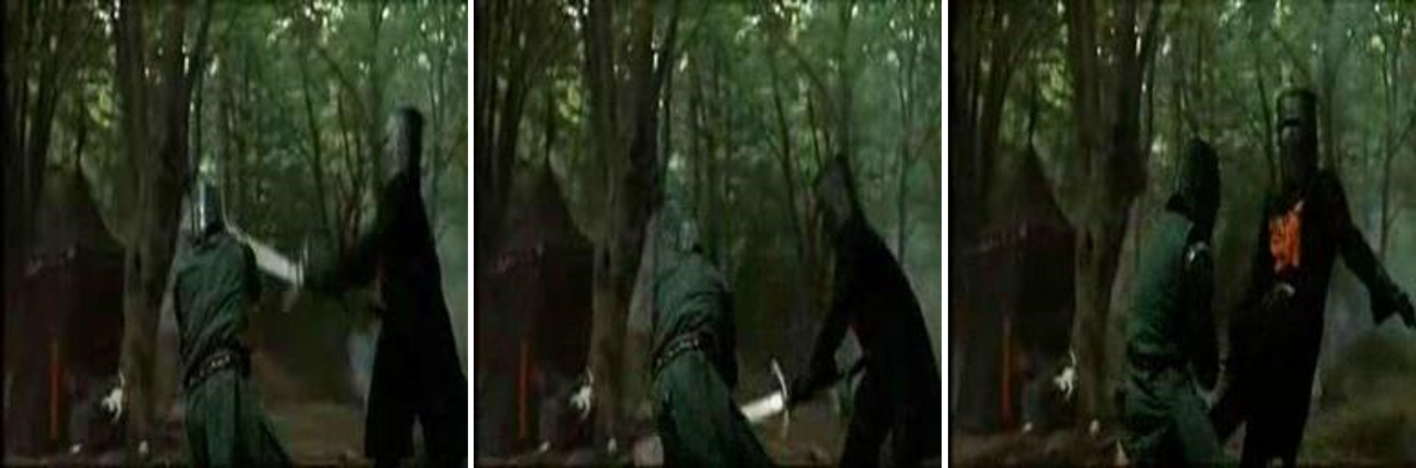
(h) labeled as ‘Kick’. (Sword?)

(i) labeled as ‘Kick’. (Ride bike?)

(j) labeled as ‘Kick’. (Turn?)

(k) labeled as ‘Sword’. (Shoot bow?)

(l) labeled as ‘Wave’. (Smile?)

Figure 11: Training examples with the highest ${\cal O(\cdot)}$ (HMDB-51). Some videos are incorrectly labeled and do not contain any scene corresponding to the label. The other videos are partly noisy and include scenes corresponding to other labels that seem more suitable. The other possible labels are shown in parentheses. (Best viewed magnified on screen.)

C.5 Experimental results after one-round

In this section, we present the results after one round of Influential Rank on CIFAR in Table 11, and on CIFAR-N in Table 12. We can observe that applying only one round of Influential Rank can considerably improve the classification accuracy. Thus, when time budget is limited, applying Influential Rank for once can be sufficient.

Appendix D Detector for Data Cleaning on Real-world Video Data

A few seconds of a video consists of a sequence of frames, ranging from tens to hundreds of consecutive images. Therefore, in general, when predicting the action class, frames are sampled and predicted for each frame. Then, the prediction scores of sampled frames are averaged and the action with the highest prediction score is determined as the final action class.

Consider a video action recognition task with $n$ training videos $(v_{1},y_{1}),\cdots,(v_{n},y_{n})$, where $v_{i}$ is the $i$th video and $y_{i}$ is its label. Let $m_{i}$ be the number of sampled frames in the $i$th video, and $x_{ij}$ be the $j$th frame in the $i$th video. Then, the empirical risk for the video dataset is given by $R(\theta)=\frac{1}{n}\sum_{i=1}^{n}(\frac{1}{m_{i}}\sum_{j=1}^{m_{i}}\ell(y_{i},f(x_{ij},\theta)))$, where $\ell(x_{ij},\theta)$ is the loss for a frame $x_{ij}$. Now, when we denote the loss of a video $v_{i}$ as $\ell(y_{i},f(v_{i},\theta))=\frac{1}{m_{i}}\sum_{j=1}^{m_{i}}\ell(y_{i},f(x_{ij},\theta))$, the empirical risk can be rewritten as $R(\theta)=\frac{1}{n}\sum_{i=1}^{n}\ell(y_{i},f(v_{i},\theta))$. Given the empirical risk $R(\theta)=\frac{1}{n}\sum_{i=1}^{n}\ell({y}_{i},f(v_{i},\theta))$, the fully optimized (overfitted) model parameters $\hat{\theta}$ minimizes the given empirical risk $R(\theta)$ as $\hat{\theta}\overset{\mathrm{def}}{=\joinrel=}\text{argmin}_{\theta}R(\theta)$. Then, a new parameter when removing the video $v$ is derived as $\hat{\theta}_{v,\omega}\overset{\mathrm{def}}{=\joinrel=}\text{argmin}_{\theta}R(\theta)+\omega\ell(y,f(v,\theta))$. Then, we can use equation (1) by definition. Therefore, a video in the video action recognition task can be easily mapped to an image in the image classification problem, and we can simply use the equations derived in this paper for the video dataset.

In this paper, we used Temporal Segment Networks (TSN) [45], which is one of the representative video action recognition models. We train the networks based on public code by Xiong , without changing the given hyperparameter settings, except the addition of a hidden layer as explained in B. We train the network for 300 epochs. We set the initial learning rate to 0.001 and drop it by a factor of 0.1 after 30 and 200 epochs. To deal with both spatial information and long-range temporal structure, TSN adopts two-stream networks that each network processes an RGB image and the stacked optical flows [14], respectively. Therefore, we compute ${\cal O}(v_{i};\hat{\theta})$ for both networks and analyze the commonly influential video clips from both networks. We present examples of the detected noisy-label videos in Figure 11.

Limitation. Although our main baseline, RoG [23], also uses validation set to optimize generative classifiers for ensemble, a limitation of our method is that it requires a small number of clean validation samples to calculate the OSD. It can be difficult to collect image data in some domains despite the limited number of 5 images per class in our experiments.

References

- [1] Héctor Allende, Rodrigo Salas, and Claudio Moraga. A robust and effective learning algorithm for feedforward neural networks based on the influence function. In Pattern Recognition and Image Analysis, pages 28–36, Berlin, Heidelberg, 2003. Springer Berlin Heidelberg.
- [2] Devansh Arpit, Stanisław Jastrzundefinedbski, Nicolas Ballas, David Krueger, Emmanuel Bengio, Maxinder S. Kanwal, Tegan Maharaj, Asja Fischer, Aaron Courville, Yoshua Bengio, and Simon Lacoste-Julien. A closer look at memorization in deep networks. In Proceedings of the 34th International Conference on Machine Learning - Volume 70, ICML’17, 2017.
- [3] Pengfei Chen, Ben Ben Liao, Guangyong Chen, and Shengyu Zhang. Understanding and utilizing deep neural networks trained with noisy labels. In International Conference on Machine Learning, pages 1062–1070, 2019.
- [4] Pengfei Chen, Junjie Ye, Guangyong Chen, Jingwei Zhao, and Pheng-Ann Heng. Beyond class-conditional assumption: A primary attempt to combat instance-dependent label noise. In International Conference on Machine Learning, 2020.
- [5] De Cheng, Tongliang Liu, Yixiong Ning, Nannan Wang, Bo Han, Gang Niu, Xinbo Gao, and Masashi Sugiyama. Instance-dependent label-noise learning with manifold-regularized transition matrix estimation. In Proceedings of the IEEE/CVF Conference on Computer Vision and Pattern Recognition (CVPR), 2022.
- [6] R. Dennis Cook and Sanford Weisberg. Residuals and Influence in Regression. 1982.
- [7] Ekin D Cubuk, Barret Zoph, Dandelion Mane, Vijay Vasudevan, and Quoc V Le. Autoaugment: Learning augmentation strategies from data. In Proceedings of the IEEE/CVF Conference on Computer Vision and Pattern Recognition, 2019.
- [8] Benoît Frénay and Michel Verleysen. Classification in the presence of label noise: a survey. IEEE transactions on neural networks and learning systems, 25(5):845–869, 2013.
- [9] Jacob Goldberger and Ehud Ben-Reuven. Training deep neural-networks using a noise adaptation layer. In 5th International Conference on Learning Representations, ICLR 2017, Toulon, France, April 24-26, 2017, Conference Track Proceedings, 2017.
- [10] F.R. Hampel. Robust Statistics: The Approach Based on Influence Functions. Probability and Statistics Series. Wiley, 1986.
- [11] Bo Han, Quanming Yao, Xingrui Yu, Gang Niu, Miao Xu, Weihua Hu, Ivor Tsang, and Masashi Sugiyama. Co-teaching: Robust training of deep neural networks with extremely noisy labels. In Advances in Neural Information Processing Systems 31, pages 8527–8537. Curran Associates, Inc., 2018.
- [12] Satoshi Hara, Atsushi Nitanda, and Takanori Maehara. Data cleansing for models trained with sgd. In Advances in Neural Information Processing Systems 32. 2019.
- [13] Dan Hendrycks, Mantas Mazeika, Duncan Wilson, and Kevin Gimpel. Using trusted data to train deep networks on labels corrupted by severe noise. In Advances in Neural Information Processing Systems 31. 2018.
- [14] Berthold K.P. Horn and Brian G. Schunck. Determining optical flow. Technical report, USA, 1980.
- [15] Jinchi Huang, Lie Qu, Rongfei Jia, and Binqiang Zhao. O2u-net: A simple noisy label detection approach for deep neural networks. In The IEEE International Conference on Computer Vision (ICCV), 2019.
- [16] Ahmet Iscen, Jack Valmadre, Anurag Arnab, and Cordelia Schmid. Learning with neighbor consistency for noisy labels. In Proceedings of the IEEE/CVF Conference on Computer Vision and Pattern Recognition (CVPR), 2022.
- [17] Lu Jiang, Zhengyuan Zhou, Thomas Leung, Li-Jia Li, and Li Fei-Fei. Mentornet: Learning data-driven curriculum for very deep neural networks on corrupted labels. In Proceedings of the 35th International Conference on Machine Learning, ICML 2018, Stockholmsmässan, Stockholm, Sweden, July 10-15, 2018, volume 80 of Proceedings of Machine Learning Research, pages 2309–2318. PMLR, 2018.
- [18] Nazmul Karim, Mamshad Nayeem Rizve, Nazanin Rahnavard, Ajmal Mian, and Mubarak Shah. Unicon: Combating label noise through uniform selection and contrastive learning. In Proceedings of the IEEE/CVF Conference on Computer Vision and Pattern Recognition (CVPR), 2022.
- [19] Andrej Karpathy, George Toderici, Sanketh Shetty, Thomas Leung, Rahul Sukthankar, and Li Fei-Fei. Large-scale video classification with convolutional neural networks. In CVPR, 2014.
- [20] Pang Wei Koh and Percy Liang. Understanding black-box predictions via influence functions. In Proceedings of the 34th International Conference on Machine Learning, pages 1885–1894, Sydney, Australia, 2017. PMLR.
- [21] A. Krizhevsky and G. Hinton. Learning multiple layers of features from tiny images. Master’s thesis, Department of Computer Science, University of Toronto, 2009.
- [22] H. Kuehne, H. Jhuang, E. Garrote, T. Poggio, and T. Serre. HMDB: a large video database for human motion recognition. In Proceedings of the International Conference on Computer Vision (ICCV), 2011.
- [23] Kimin Lee, Sukmin Yun, Kibok Lee, Honglak Lee, Bo Li, and Jinwoo Shin. Robust inference via generative classifiers for handling noisy labels. In International Conference on Machine Learning. PMLR, 2019.
- [24] Junnan Li, Richard Socher, and Steven CH Hoi. Dividemix: Learning with noisy labels as semi-supervised learning. In International Conference on Learning Representations, 2020.
- [25] Junnan Li, Yongkang Wong, Qi Zhao, and Mohan S. Kankanhalli. Learning to learn from noisy labeled data. In Proceedings of the IEEE/CVF Conference on Computer Vision and Pattern Recognition (CVPR), June 2019.
- [26] Mingchen Li, Mahdi Soltanolkotabi, and Samet Oymak. Gradient descent with early stopping is provably robust to label noise for overparameterized neural networks. In International conference on artificial intelligence and statistics, pages 4313–4324. PMLR, 2020.
- [27] Wen Li, Limin Wang, Wei Li, Eirikur Agustsson, and Luc Van Gool. Webvision database: Visual learning and understanding from web data. arXiv preprint arXiv:1708.02862, 2017.
- [28] Xuefeng Li, Tongliang Liu, Bo Han, Gang Niu, and Masashi Sugiyama. Provably end-to-end label-noise learning without anchor points. In Proceedings of the 38th International Conference on Machine Learning. PMLR, 2021.
- [29] Sheng Liu, Jonathan Niles-Weed, Narges Razavian, and Carlos Fernandez-Granda. Early-learning regularization prevents memorization of noisy labels. Advances in Neural Information Processing Systems, 33, 2020.
- [30] Yang Liu and Hongyi Guo. Peer loss functions: Learning from noisy labels without knowing noise rates. In International Conference on Machine Learning, pages 6226–6236, 2020.
- [31] Xingjun Ma, Hanxun Huang, Yisen Wang, Simone Romano, Sarah Erfani, and James Bailey. Normalized loss functions for deep learning with noisy labels. In International Conference on Machine Learning, pages 6543–6553, 2020.
- [32] Feng Mao, Xiang Wu, Hui Xue, and Rong Zhang. Hierarchical video frame sequence representation with deep convolutional graph network. In Proceedings of the European Conference on Computer Vision (ECCV) Workshops, pages 0–0, 2018.
- [33] Nagarajan Natarajan, Inderjit S Dhillon, Pradeep K Ravikumar, and Ambuj Tewari. Learning with noisy labels. In Advances in Neural Information Processing Systems 26. 2013.
- [34] Duc Tam Nguyen, Chaithanya Kumar Mummadi, Thi Phuong Nhung Ngo, Thi Hoai Phuong Nguyen, Laura Beggel, and Thomas Brox. SELF: Learning to filter noisy labels with self-ensembling. In International Conference on Learning Representations, 2020.
- [35] Giorgio Patrini, Alessandro Rozza, Aditya Krishna Menon, Richard Nock, and Lizhen Qu. Making deep neural networks robust to label noise: A loss correction approach. In The IEEE Conference on Computer Vision and Pattern Recognition (CVPR), 2017.
- [36] Olga Russakovsky, Jia Deng, Hao Su, Jonathan Krause, Sanjeev Satheesh, Sean Ma, Zhiheng Huang, Andrej Karpathy, Aditya Khosla, Michael Bernstein, Alexander C. Berg, and Li Fei-Fei. ImageNet Large Scale Visual Recognition Challenge. International Journal of Computer Vision (IJCV), 2015.
- [37] Karen Simonyan and Andrew Zisserman. Two-stream convolutional networks for action recognition in videos. In Advances in Neural Information Processing Systems 27: Annual Conference on Neural Information Processing Systems 2014, December 8-13 2014, Montreal, Quebec, Canada, pages 568–576, 2014.
- [38] Hwanjun Song, Minseok Kim, and Jae-Gil Lee. SELFIE: Refurbishing unclean samples for robust deep learning. In Proceedings of the 36th International Conference on Machine Learning. PMLR, 2019.
- [39] Hwanjun Song, Minseok Kim, Dongmin Park, and Jae-Gil Lee. How does early stopping help generalization against label noise? In International Conference on Machine Learning Workshop, 2020.
- [40] Hwanjun Song, Minseok Kim, Dongmin Park, Yooju Shin, and Jae-Gil Lee. Learning from noisy labels with deep neural networks: A survey. IEEE Transactions on Neural Networks and Learning Systems, 2022.
- [41] Nitish Srivastava, Geoffrey Hinton, Alex Krizhevsky, Ilya Sutskever, and Ruslan Salakhutdinov. Dropout: A simple way to prevent neural networks from overfitting. Journal of Machine Learning Research, 15:1929–1958, 2014.
- [42] Zeren Sun, Fumin Shen, Dan Huang, Qiong Wang, Xiangbo Shu, Yazhou Yao, and Jinhui Tang. Pnp: Robust learning from noisy labels by probabilistic noise prediction. In Proceedings of the IEEE/CVF Conference on Computer Vision and Pattern Recognition (CVPR), 2022.
- [43] Christian Szegedy, Sergey Ioffe, Vincent Vanhoucke, and Alexander A. Alemi. Inception-v4, inception-resnet and the impact of residual connections on learning. In Proceedings of the Thirty-First AAAI Conference on Artificial Intelligence, AAAI’17, 2017.
- [44] Daiki Tanaka, Daiki Ikami, Toshihiko Yamasaki, and Kiyoharu Aizawa. Joint optimization framework for learning with noisy labels. In CVPR, 2018.
- [45] Limin Wang, Yuanjun Xiong, Zhe Wang, Yu Qiao, Dahua Lin, Xiaoou Tang, and Luc Van Gool. Temporal segment networks: Towards good practices for deep action recognition. In Computer Vision - ECCV 2016 - 14th European Conference, Amsterdam, The Netherlands, October 11-14, 2016, Proceedings, Part VIII, pages 20–36, 2016.
- [46] Jiaheng Wei, Zhaowei Zhu, Hao Cheng, Tongliang Liu, Gang Niu, and Yang Liu. Learning with noisy labels revisited: A study using real-world human annotations. In International Conference on Learning Representation, 2022.
- [47] Chao-Yuan Wu and Philipp Krahenbuhl. Towards long-form video understanding. In Proceedings of the IEEE/CVF Conference on Computer Vision and Pattern Recognition (CVPR), pages 1884–1894, June 2021.
- [48] Tong Xiao, Tian Xia, Yi Yang, Chang Huang, and Xiaogang Wang. Learning from massive noisy labeled data for image classification. In The IEEE Conference on Computer Vision and Pattern Recognition (CVPR), 2015.
- [49] Yilun Xu, Peng Cao, Yuqing Kong, and Yizhou Wang. L_dmi: A novel information-theoretic loss function for training deep nets robust to label noise. In Advances in Neural Information Processing Systems 32. 2019.
- [50] Kun Yi and Jianxin Wu. Probabilistic end-to-end noise correction for learning with noisy labels. In The IEEE Conference on Computer Vision and Pattern Recognition (CVPR), 2019.
- [51] Xingrui Yu, Bo Han, Jiangchao Yao, Gang Niu, Ivor W. Tsang, and Masashi Sugiyama. How does disagreement help generalization against label corruption? In Proceedings of the 36th International Conference on Machine Learning, ICML 2019, 9-15 June 2019, Long Beach, California, USA. PMLR, 2019.
- [52] Chiyuan Zhang, Samy Bengio, Moritz Hardt, Benjamin Recht, and Oriol Vinyals. Understanding deep learning requires rethinking generalization. In 5th International Conference on Learning Representations, ICLR 2017, Toulon, France, April 24-26, 2017, Conference Track Proceedings, 2017.
- [53] Hongyi Zhang, Moustapha Cisse, Yann N Dauphin, and David Lopez-Paz. mixup: Beyond empirical risk minimization. In International Conference on Learning Representations, 2018.
- [54] Weihe Zhang, Yali Wang, and Yu Qiao. Metacleaner: Learning to hallucinate clean representations for noisy-labeled visual recognition. In Proceedings of the IEEE/CVF Conference on Computer Vision and Pattern Recognition (CVPR), June 2019.
- [55] Zhilu Zhang and Mert Sabuncu. Generalized cross entropy loss for training deep neural networks with noisy labels. In Advances in Neural Information Processing Systems 31. Curran Associates, Inc., 2018.
- [56] Zizhao Zhang, Han Zhang, Sercan O Arik, Honglak Lee, and Tomas Pfister. Distilling effective supervision from severe label noise. In Proceedings of the IEEE/CVF Conference on Computer Vision and Pattern Recognition, pages 9294–9303, 2020.
- [57] Songzhu Zheng, Pengxiang Wu, Aman Goswami, Mayank Goswami, Dimitris Metaxas, and Chao Chen. Error-bounded correction of noisy labels. In Hal Daumé III and Aarti Singh, editors, Proceedings of the 37th International Conference on Machine Learning, pages 11447–11457. PMLR, 2020.
- [58] Tianyi Zhou, Shengjie Wang, and Jeff Bilmes. Robust curriculum learning: From clean label detection to noisy label self-correction. In International Conference on Learning Representations, 2021.