Backdoor Learning Curves: Explaining Backdoor Poisoning Beyond Influence Functions

Abstract

Backdoor attacks inject poisoning samples during training, with the goal of forcing a machine learning model to output an attacker-chosen class when presented a specific trigger at test time. Although backdoor attacks have been demonstrated in a variety of settings and against different models, the factors affecting their effectiveness are still not well understood. In this work, we provide a unifying framework to study the process of backdoor learning under the lens of incremental learning and influence functions. We show that the effectiveness of backdoor attacks depends on: (i) the complexity of the learning algorithm, controlled by its hyperparameters; (ii) the fraction of backdoor samples injected into the training set; and (iii) the size and visibility of the backdoor trigger. These factors affect how fast a model learns to correlate the presence of the backdoor trigger with the target class. Our analysis unveils the intriguing existence of a region in the hyperparameter space in which the accuracy on clean test samples is still high while backdoor attacks are ineffective, thereby suggesting novel criteria to improve existing defenses.

Keywords backdoor poisoning;influence functions;data poisoning;machine learning;adversarial machine learning;secure machine learning;security

1 Introduction

Machine learning models are vulnerable to backdoor poisoning  [1, 2]. These attacks consist in injecting poisoning samples at training time, with the goal of forcing the trained model to output an attacker-chosen class when presented a specific trigger at test time, while working as expected otherwise. To this end, the poisoning samples typically need not only to embed such a backdoor trigger themselves, but also to be labeled as the attacker-chosen class. As backdoor poisoning preserves model performance on clean test data, it is not straightforward for the victim to realize that the model has been compromised.

Backdoor poisoning has been demonstrated in a plethora of different scenarios. In one pertinent setting, the user is assumed to download a pre-trained, backdoored model from an untrusted source, to subsequently fine-tune it on their data. As backdoors typically remain effective even after this fine-tuning step, they may successfully be exploited by the attacker at test time [2, 1]. Alternatively, the attacker is assumed to alter part of the training data collected by the user, either to train the model from scratch or to fine-tune a pre-trained model via transfer learning [3, 4]. In such cases, the training labels of poisoning samples may be either fully controlled by the attacker [3] or subject to validation by the victim [4], depending on the considered threat model. Backdoor attacks have been shown to be effective in different applications and against a variety of models, including vision [1] and language models [5], graph neural networks [6], and even reinforcement learning [7]. However, it is still unclear which factors influence the ability of a model to learn a backdoor, i.e., to classify the test samples containing the backdoor trigger as the attacker-chosen class.

In this work, we analyze the process of backdoor learning to identify the main factors affecting the vulnerability of machine learning models against this attack. To this end, we propose a framework that characterizes the backdoor learning process. The learning process of humans is usually characterized using learning curves, a graphical representation of the relationship between the hours spent practicing and the proficiency to accomplish a given task. Inspired by this concept, we introduce the notion of backdoor learning curves (Sect. 2). To generate these curves, we formulate backdoor learning as an incremental learning problem and assess how the loss on the backdoor samples decreases as they are gradually learned by the target model. These backdoor learning curves are independent from a threat model in so far as they capture both training data and fine-tuning attacks. We show that the slope of this curve, the backdoor learning slope, which is connected to the notion of influence functions, quantifies the speed with which the model learns the backdoor samples and hence its vulnerability. Additionally, to provide further insights about the backdoor’s influence on the learned classifiers, we propose a way to quantify the backdoor impact on learning parameters, i.e., how much the parameters of a model deviate from the initial values when the model learns a backdoor.

Our experimental analysis (Sect. 3) shows that the factors influencing the success of backdoor poisoning are: (i) the fraction of backdoor samples injected into the training data; (ii) the size of the backdoor trigger; and (iii) the complexity of the target model, controlled via its hyperparameters. Concerning the latter, our experimental findings reveal a region in the hyperparameter space where models are highly accurate on clean samples while also being robust to backdoor poisoning. This region exists as, to learn a backdoor, the target model is required to significantly increase the complexity of its decision function, and this is not possible if the model is sufficiently regularized. This observation will help identify novel criteria to improve existing defenses and inspire new countermeasures.

To summarize, the main contributions of this work are:

• We introduce backdoor learning curves as a powerful tool to thoroughly characterize the backdoor learning process;

• We introduce a metric, named backdoor learning slope, to quantify the ability of the classifier to learn backdoors;

• We identify three important factors that affect the vulnerability against backdoors;

• We unveil a region in the hyperparameter space in which the classifiers are highly accurate and robust against backdoors, which supports novel defensive strategies.

We conclude the paper by discussing related work in Sect. 4, along with the limitations of our approach and promising future research directions in Sect. 5.

2 Backdoor Learning Curves

In this section, we introduce our framework to characterize backdoor poisoning by means of learning curves and their slope. Afterwards, we introduce two measures to quantify the backdoor impact on the model’s parameters.

Notation. We denote the input data and their labels respectively with $\boldsymbol{x}\in\mathbb{R}^{d}$ and $y\in\{1,..,c\}$, being $c$ the number of classes. We refer to the untainted, clean training data as $\mathcal{D}_{\rm tr}=(\boldsymbol{x}_{i},y_{i})_{i=1}^{n}$, and to the backdoor samples injected into the training set as $\mathcal{P}_{\rm tr}=(\hat{\boldsymbol{x}}_{j},\hat{y}_{j})_{j=1}^{m}$. We refer to the clean test samples as $\mathcal{D}_{\rm ts}=({\boldsymbol{x}}_{t},{y}_{t})_{t=1}^{k}$ and to the test samples containing the backdoor trigger as $\mathcal{P}_{\rm ts}=(\hat{\boldsymbol{x}}_{t},\hat{y}_{t})_{t=1}^{k}$.

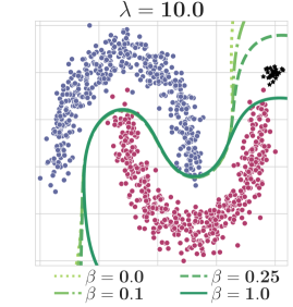
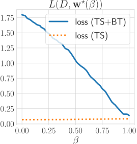
(a) Strong regularization ($\lambda=10$).

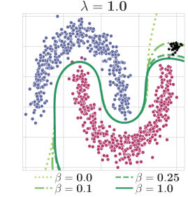
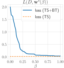
(b) Weak regularization ($\lambda=1$).

Figure 1: Backdoor learning curves and their relationship with model complexity. Considering an SVM with an RBF kernel ($\gamma=10.0$) on a toy dataset in two dimensions, we show the influence of model complexity (controlled by $\lambda$, set to $10$ (left) and $1$ (right)). For each setting, we created two plots. The left plot shows on a 2-dimensional plane the data (dots) and decision surface for different values of $\beta$ (green lines). The right plot shows the backdoor learning curve, where the y-axis represents the classifier’s loss and the x-axis $\beta$. We plot both the loss on the clean test data (orange dotted line) and the test dataset containing the backdoor trigger (blue line). The slope of these curves represents the speed with which the model learns the backdoored samples (black dots), labeled as blue class. The model on the left struggles to fit the backdoors and succeeds only with high $\beta$, whereas the one on the right already fits the model at low $\beta$.

Backdoor Learning Curves. We leverage previous work from incremental learning [8, 9] to study how gradually incorporating backdoor samples affects the learned classifier. In mathematical terms, we formalize the learning problem as:

$$\begin{split}\boldsymbol{w}^{\star}(\beta)\in&\operatornamewithlimits{\arg\,\min}_{\boldsymbol{w}}\mathcal{L}(D_{\rm tr}\cup\mathcal{P}_{\rm tr},\boldsymbol{w})=L(D_{\rm tr},\boldsymbol{w})+\beta L(\mathcal{P}_{\rm tr},\boldsymbol{w})+\lambda\Omega(\boldsymbol{w})\,,\end{split}$$ (1)

where $L$ is the loss attained on a given dataset by the classifier with parameters $\boldsymbol{w}$. $\mathcal{L}$ is the loss computed on the training points and the backdoor samples, which also includes a regularization term $\Omega(\boldsymbol{w})$ (e.g., $\|\boldsymbol{w}\|^{2}_{2}$), weighed by the regularization hyperparameter $\lambda$. To gradually incorporate the backdoor samples, we use $\beta\in[0,1]$. It regulates the weight the classifier gives to the loss on the samples with backdoor trigger. As $\beta$ ranges from 0 (unpoisoned classifier) to 1 (poisoned classifier), the classifier gradually learns the backdoor by adjusting its parameters. For this reason, we make the dependency of the optimal weights $\boldsymbol{w}^{\star}$ on $\beta$ explicit as $\boldsymbol{w}^{\star}(\beta)$.

We now define the backdoor learning curve as the curve showing the behavior of the classifier loss $L(\mathcal{P}_{\rm ts},\boldsymbol{w}^{\star}(\beta))$ on the test samples with the backdoor trigger as a function of $\beta$. In the following, we abbreviate $L(\mathcal{P}_{\rm ts},\boldsymbol{w}^{\star}(\beta))$ as $L$. Intuitively, the faster the backdoor learning curve decreases, the easier the target model is backdoored. The exact details of how the model is backdoored do not matter for this analysis, e.g. our approach captures for example both the setting where the training data is altered as well as the setting where fine-tuning data is tampered with.

We give an example of two such curves under different regularizations in Figure 1. The left plots depict a strongly regularized classifier. The corresponding backdoor learning curve (on the right) shows that the classifier achieves low loss and high accuracy on the backdoor samples only after poisoning (when $\beta=1$), namely when the loss on the backdoor samples is considered equally important to the loss on the training samples. The classifier on the right, instead, is less regularized and thus more complex. Consequently, this classifier learns to incorporate the backdoor samples much faster (at low $\beta$), namely when the loss on the backdoor points is taken into account less than the one on the training data. This highlights that this classifier is probably more vulnerable to this attack.

Backdoor Learning Slope.We quantify how fast an untainted classifier can be poisoned by proposing a novel measure, namely the backdoor learning slope, that measures the velocity with which the classifier learns to classify the backdoor samples correctly. This measure allows us to compare the vulnerability of a classifier trained with different hyperparameters or considering different poisoning scenarios (e.g. when the attacker can inject a different number of poisoning points or creating triggers with different sizes), allowing us to identify factors relevant to backdoor learning. Moreover, as we will show, this measure can be used by the system designer to choose an appropriate combination of hyperparameters for the task at hand. To this end, we define the backdoor learning slope as the gradient of the backdoor learning curve at $\beta=0$, capturing the velocity of the curve on learning the backdoor. Formally, the backdoor learning slope can be formulated as follow:

$$\frac{\partial L(\mathcal{P}_{\rm ts},\boldsymbol{w}^{\star}(\beta))}{\partial\beta}=\frac{\partial L}{\partial\boldsymbol{w}}\frac{\partial\boldsymbol{w}^{\star}}{\partial\beta}\,,$$ (2)

where the first term is straightforward to compute, and the second term implicitly captures the dependency of the optimal weights on the hyperparameter $\beta$. In other words, it requires us to understand how the optimal classifier parameters change when gradually increasing $\beta$ from 0 to 1, i.e., while incorporating the backdoor samples into the learning process.

To compute this term, as suggested in previous work in incremental learning [8], we assume that, while increasing $\beta$, the solution maintains the optimality (Karush-Kuhn-Tucker, KKT) conditions intact. This equilibrium implies that $\nabla_{\beta}\nabla_{\boldsymbol{w}}\mathcal{L}(\boldsymbol{w}^{\star})+\frac{\partial\boldsymbol{w}^{\star}}{\partial\beta}\nabla^{2}_{\boldsymbol{w}}\mathcal{L}(\boldsymbol{w}^{\star})=\boldsymbol{0}$. Based on this condition, we obtain the derivative of interest,

$$\frac{\partial\boldsymbol{w}^{\star}}{\partial\beta}=-(\nabla^{2}_{\boldsymbol{w}}\mathcal{L}(\boldsymbol{w}^{\star}))^{-1}\cdot\nabla_{\beta}\nabla_{\boldsymbol{w}}\mathcal{L}(\boldsymbol{w}^{\star})\,.$$ (3)

Substituting it in Eq. 2 we obtain the complete gradient:

$$\frac{\partial L(\mathcal{P}_{\rm ts},\boldsymbol{w}^{\star}(\beta))}{\partial\beta}=-\nabla_{\boldsymbol{w}}L\cdot(\nabla^{2}_{\boldsymbol{w}}\mathcal{L})^{-1}\cdot\nabla_{\beta}\nabla_{\boldsymbol{w}}\mathcal{L}\,.$$ (4)

The gradient in Eq. 4 corresponds to the sum of the pairwise influence function values $\mathcal{I}_{\rm up,loss}(\boldsymbol{x}_{\rm tr},\boldsymbol{x}_{\rm ts})$ used by [10]. The authors indeed proposed to measure how relevant a training point is for the predictions of a given test point by computing $\left.\frac{\partial L}{\partial\beta}\right|_{\beta=0}=\sum_{t}\sum_{j}\mathcal{I}_{\rm up,loss}(\hat{\boldsymbol{x}}_{t},\hat{\boldsymbol{x}}_{j})$. To understand how this gradient can be efficiently computed via Hessian-vector products and other approximations, we refer the reader to [10] as well as to recent developments in gradient-based bilevel optimization [11, 12, 13, 14, 15].

The main difference between the approach by [10] and ours stems from their implicit treatment of regularization and our interest in understanding vulnerability to a subset of backdoor training points, rather than in providing prototype-based explanations. However, directly using the gradient of the loss wrt. $\beta$ comes with two disadvantages. First, the slope is inverse to $\beta$ and second, to obtain results comparable across classifiers, we need to rescale the slope. We thus transform the gradient as:

$$~{}\theta=-\frac{2}{\pi}\arctan{\left(\left.\frac{\partial L}{\partial\beta}\right|_{\beta=0}\right)}\in[-1,1]\,,$$ (5)

where we use the negative sign to have positive values correlated with faster backdoor learning (i.e., the loss decreases faster as $\beta$ grows). Computing $\nicefrac{{2}}{{$\pi$}}$ of the gradient allows us to rescale the slope to be in the interval between $[-1,1]$. Hence, a value around $0$ implies that the loss of the backdoor samples does not decrease. In other words, the classifier does not learn the backdoor trigger and is hence very robust.

Backdoor Impact on Learning Parameters. After introducing the previous plot and measure, we are able to quantify how backdoors are learned by the model. To provide further insights about the backdoor’s influence on the learned classifier, we propose to monitor how the classifier’s parameters deviate from their initial, unbackdoored values once a backdoor is added. Our approach below captures only convex learners. As shown by Zhang et al. [16], the impact of a network weight in non-convex classifiers’ decision depends on the layer of which it is part. Therefore, measuring the parameter deviation in the non-convex case is challenging, and we leave this unsolved problem for future work.

To capture backdoor impact on learning parameters in the convex case, we consider the initial weights $\boldsymbol{w}_{0}=\boldsymbol{w}^{\star}(\beta=0)$ and $\boldsymbol{w}_{\beta}=\boldsymbol{w}^{\star}(\beta)$ for $\beta>0$, and measure two quantities:

$$\rho=\|\boldsymbol{w}_{\beta}\|\in[0,\infty),\;{\rm and}\;\nu=\frac{1}{2}\left(1-\frac{\boldsymbol{w}_{0}^{\top}\boldsymbol{w}_{\beta}}{\|\boldsymbol{w}_{0}\|\|\boldsymbol{w}_{\beta}\|}\right)\in[0,1]\,.$$ (6)

The first measure, $\rho$, quantifies the change of the weights when $\beta$ increases. This quantity is equivalent to the regularization term used for learning. The second one, $\nu$, quantifies the change in orientation of the classifier. In a nutshell, we compute the angle between the two vectors and rescale it to be in the interval of $[0,1]$. Both metrics are defined to grow as $\beta\rightarrow 1$, in other words as the backdoored classifier deviates more and more from the original classifier. Consequently, in the empirical parameter deviation plots in Section 3.2, we report the value of $\rho(\nu)$ (on the y-axis) as $\beta$ (on the x-axis) varies from 0 to 1, to show how the classifier parameters are affected by backdoor learning.

3 Experiments

Employing the previously proposed methodology, we carried out an empirical analysis on linear and nonlinear classifiers. In this section, we start with the experiments aimed to study the impact of different factors on backdoor learning. To this end, we employ the backdoor learning curves and the backdoor learning slope to study how the capacity of the model to learn backdoors changes when (a) varying the model’s complexity, defined by its hyperparameters, (b) the attacker’s strength, defined by the percentage of poisoning samples in the training set and (c) the trigger size and visibility. Our results show that these components significantly determine how fast the backdoor is learned, and consequently, the model’s vulnerability. Then, leveraging the proposed measures to analyze how the classifier’s parameters change during backdoor learning, we provide further insights on the effect of the aforementioned factors on the trained model. The results presented in this section will help identify novel criteria to improve existing defenses and inspire new countermeasures. The source code is available on the author’s GitHub page.

3.1 Experimental Setup

Our work investigates which factors influence backdoor vulnerability considering convex-learners and neural networks. In the following, we describe our datasets, models, and the backdoor attacks studied in our experiments.

Datasets. We carried out our experiments on the MNIST [17], CIFAR10 [18] and Imagenette [19] datasets. When adopting convex-learners we consider the two-class subproblems as in the work by Saha et al. [4] and Suya et al. [20]. On MNIST, we choose the pairs $7~{}\rm{vs}~{}1$, $3~{}\rm{vs}~{}0$, and $5~{}\rm{vs}~{}2$, as our models exhibited the highest clean accuracy on these pairs. On CIFAR10, analogous to prior work [4], we choose airplane vs frog, bird vs dog, and airplane vs truck. On Imagenette we randomly choose tench vs truck, cassette player vs church, and tench vs parachute. For each two-class subtask we use $1500$ and $500$ samples as training and test set respectively. In the following section, we focus on the results of one pair on each dataset: $7~{}\rm{vs}~{}1$ on MNIST, airplane vs frog on CIFAR10, and tench vs truck on Imagenette. The results of the other pairs (reported in  A.1) are analogous. When testing our framework against neural networks, we train on all the ten classes of Imagenette. We use $70\%$ and $30\%$ of the entire dataset for training and test, respectively.

Models and Training phase. To thoroughly analyze how learning a backdoor affects a model, we consider different convex learning algorithms, including linear Support Vector Machines (SVMs), Logistic Regression Classifiers (LCs), Ridge Classifiers (RCs) and nonlinear SVMs using the Radial Basis Function (RBF) kernel, and deep neural networks. We train the classifiers directly on the pixel values scaled in the range $[0,1]$ on the MNIST dataset. For CIFAR10 and Imagenette, we instead consider a transfer learning setting frequently adopted in the literature [21, 22, 10]. Like Saha et al. [4], we use the pre-trained model AlexNet [23] as a feature extractor. The convex-learners are then trained on top of the feature extractor. We study these convex learners due to their broad usage in industry [20], derived from their low computational cost, excellent results, and good interpretability [24, 25].

Regarding the considered deep neural networks, we use pretrained Resnet18 and Resnet50 which are among the most widely used architectures [16]. We fine-tune them on the Imagenette dataset.

Hyperparameters.  The choice of hyperparameters has a relevant impact on the learned decision function. For example, some of these parameters control the complexity of the learned function, which may lead to overfitting [26], thereby potentially compromising classification accuracy on test samples. We argue that a high complexity may also lead to higher importance to outlying samples, including backdoors, and thus has a crucial impact on the capacity of the model to learn backdoors. To verify our hypothesis, we consider different configurations of the models’ hyperparameters. For convex-learners we consider two hyperparameters that impact model complexity, i.e., the regularization hyperparameter $\lambda$ and the RBF kernel hyperparameter $\gamma$. To this end, we take 10 values for $\lambda$ on a uniformly spaced interval on a log scale from ${1}\mathrm{e}{-04}$ to ${1}\mathrm{e}{+02}$. For the Imagenette dataset we extend this interval in $[{1}\mathrm{e}{-05},{1}\mathrm{e}{+02}]$. Concerning the RBF kernel, we let $\gamma$ take $5$ uniformly spaced values on a log scale in $[{5}\mathrm{e}{-04},{5}\mathrm{e}{-02}]$ for MNIST, $[{1}\mathrm{e}{-04},{1}\mathrm{e}{-02}]$ for CIFAR, and $[{1}\mathrm{e}{-05},{1}\mathrm{e}{-03}]$ for Imagenette. Furthermore, we take $10$ values of $\lambda$ in the log scale uniformly spaced interval $[{1}\mathrm{e}{-01},{1}\mathrm{e}{+02}]$ for the RBF kernel. This allowed us to study a combination of $10$ and $50$ hyperparameters for linear classifiers and RBF SVM respectively.

For deep neural networks, we consider two different numbers of epochs: $10$ and $50$, and increase the number of neurons when using Resnet50 instead of Resnet18. Whereas size intuitively correlates with complexity, previous works, including [27], show that decreasing the number of training epochs reduces the complexity of the trained network as well. Conversely, increasing epochs leads to overfitting on the training dataset, thus a more complex decision function. Each network is fine-tuned using the SGD optimizer with a learning rate of $0.001$, a momentum of $0.9$, and batch size $256$.

Backdoor Attacks. We implement the backdoor attacks proposed by Gu et al. [1] against MNIST and CIFAR10. More concretely, we use a random $3\times 3$ patch as the trigger for MNIST, while on CIFAR10, we increase the size to $8\times 8$ to strengthen the attack [4]. We add the trigger pattern in the lower right corner of the image [1]. Samples from MNIST and CIFAR10 with and without trigger can be found in Figure 12. However, in contrast to previous approaches [1], we use a separate trigger for each base-class $i$. The reason is that our study encompasses linear models that are unable to associate the same trigger pattern to two different classes. Using different trigger patterns, we enhance the effectiveness of the attack on these linear models. On the Imagenette dataset, we use the backdoor trigger developed by [28]. This attack consists of injecting a patterned perturbation mask into training samples to open the backdoor. A constant value $c_{m}$ refers to the maximum allowed intensity. We apply the backdoor attacks by altering 10% of the training data if not stated otherwise, and, as done by Gu et al. [1], we force the backdoored model to predict the $i$-th class as class $(i+1)\%n\_classes$ when the trigger is shown. We also report additional experiments concerning variations in the trigger’s size or visibility.

3.2 Experimental Results

In the following we now discuss our experimental results obtained with the datasets, classifiers and backdoor attacks described above.

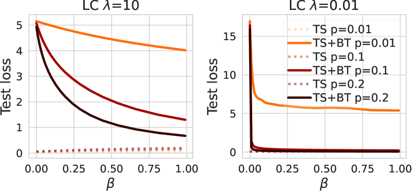
(a) MNIST trigger size $3\times 3$.

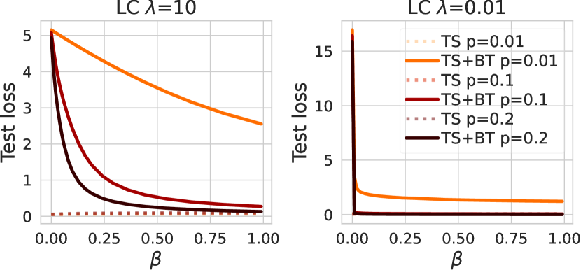
(b) MNIST trigger size $6\times 6$.

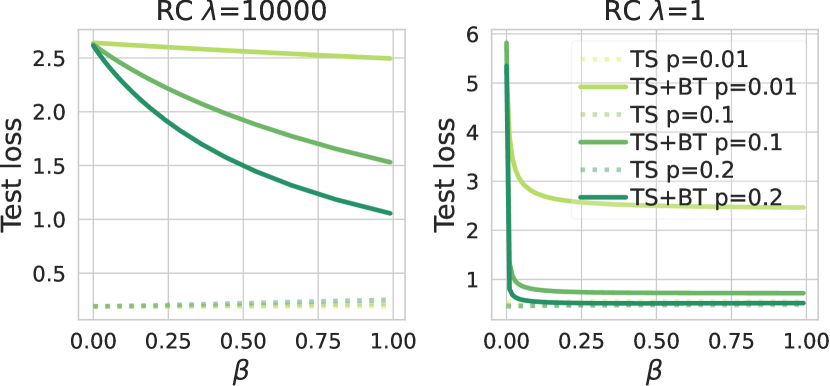
(c) CIFAR10 trigger size $8\times 8$.

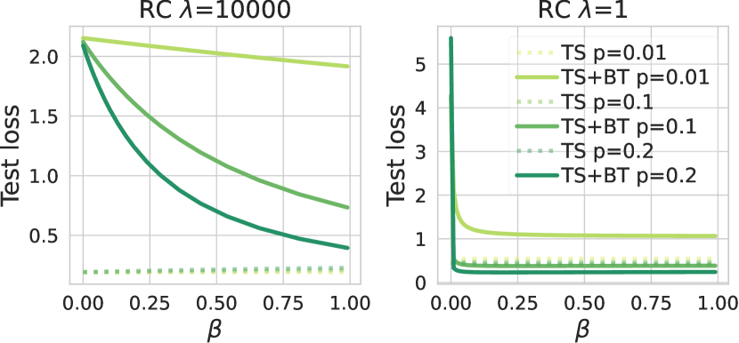
(d) CIFAR10 trigger size $16\times 16$.

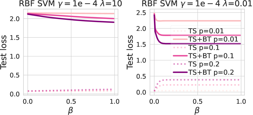
(e) Imagenette trigger visibility $c_{m}=10$.

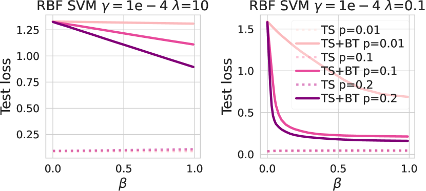
(f) Imagenette trigger visibility $c_{m}=75$.

Figure 2: Backdoor learning curves for: (top row) logistic classifier (LC) on MNIST 7 vs. 1 with $\lambda\in\{10,0.01\}$ and trigger size $3\times 3$ (left) or $6\times 6$ (right); (middle row) Ridge classifier on CIFAR10 airplane vs frog with $\lambda\in\{100000,100\}$ and trigger size $8\times 8$ (left) or $16\times 16$ (right); (bottom row) RBF SVM with $\gamma={1}\mathrm{e}{-04}$ on Imagenette tench vs truck with $\lambda\in\{10,0.1\}$ and trigger visibility $c_{m}=10$ (left) or $c_{m}=75$ (right). Darker lines represent a higher fraction of poisoning samples $p$ injected into the training set. We report the loss on the clean test samples (TS) with a dashed line and on the test samples with the backdoor trigger (TS+BT) with a solid line.

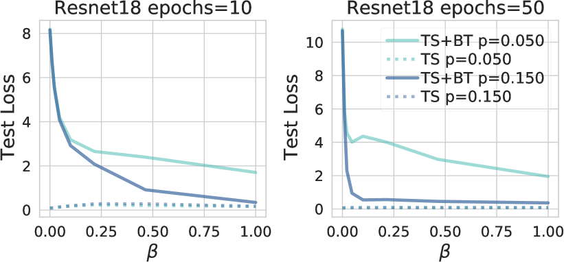
(a) Imagenette with trigger visibility $c_{m}=10$.

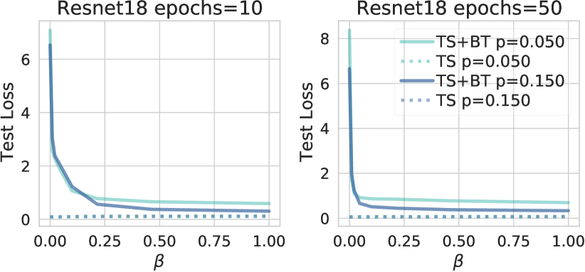
(b) Imagenette with trigger visibility $c_{m}=75$.

Figure 3: Backdoor learning curves for Resnet18 trained on the full Imagenette training dataset with $10$ and $50$ epochs. Darker lines represent a higher fraction of poisoning samples $p$ injected into the training set. We report the loss on the clean test samples (TS) with a dashed line and on the test samples with the backdoor trigger (TS+BT) with a solid line.

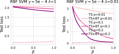
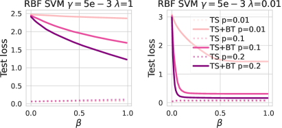
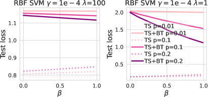
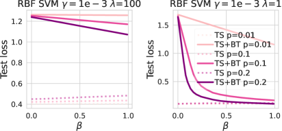
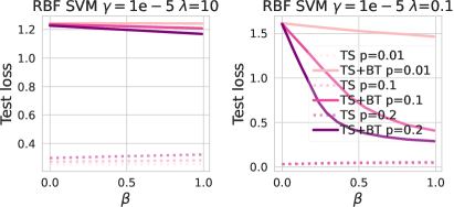
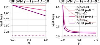
Figure 4: Backdoor learning curves for MNIST $7~{}\rm{vs}~{}1$ (top row), CIFAR10 airplane vs frog (middle row) and Imagenette tench vs truck (bottom row) when changing the kernel parameter $\gamma$ on RBF SVM. Darker lines represent a higher fraction of poisoning samples $p$ injected into the training set. We report the loss on the clean test samples (TS) with a dashed line and on the test samples with the backdoor trigger (TS+BT) with a solid line.

Backdoor Learning Curves. Here we present the results obtained using the learning curves that we proposed to study the impact of three different factors on the backdoor learning process: (i) model complexity, (ii) the fraction of backdoor samples injected, and (iii) the size and visibility of the backdoor trigger. We report the impact of the these factors on the backdoor learning curves in Figure 2 and 3.

More specifically, in Figure 2 we consider convex classifiers (i.e. LC, RC and RBF SVM) trained on two-class subproblems (MNIST, CIFAR10 and Imagenette), whereas in Figure 3 we show the results for Resnet18 trained on all the ten classes of Imagenette. To analyze the first factor, we report the results on the same classifiers, changing the hyperparameters that influence their corresponding complexity. In the case of convex-learners, we test different values of the regularization coefficient, while for Resnet18, we increase the number of epochs.

To analyze the impact of the second factor, we plot the backdoor learning curves when the attacker injects an increasing percentage of poisoning points $p\in\{0.01,0.1,0.2\}$ for convex learners and $p\in\{0.05,0.15\}$ for Resnet18. Finally, to study the third factor, namely the size and visibility of the backdoor trigger, we have created the same backdoor curves doubling the size of the patch triggers for MNIST and CIFAR10, and increasing the trigger’s visibility for Imagenette. Even when a high percentage of poisoning points are injected, for flexible enough classifiers, the loss on the clean test samples remains almost constant. Instead, the loss on the test set containing the backdoor trigger is highly affected by the factors mentioned above. Both a smaller $\lambda$ or a larger number of epochs (low regularization and thus higher complexity), and larger $p$ (a high percentage of poisoning points added) increase the slope of the backdoor learning curve. This means that the classifier learns the backdoor faster. When the classifier is sufficiently complex, even a low percentage of low poisoning points suffices to make the classifier learn the backdoor rapidly. On the other hand, this does not hold for highly regularized classifiers, which generally learn backdoors slowly. Therefore, limiting the classifier complexity by choosing an appropriate regularization coefficient may reduce the vulnerability against backdoors. Moreover, our results show that if the size of the trigger is large, the classifiers learn the backdoor faster, especially if they are complex. The same conclusion holds when increasing the trigger’s visibility, thus shedding light on the familiar trade-off between attacker’s strength vs. detectability introduced by Frederickson et al. [29]. The attacker can increase the trigger size or increase the trigger’s visibility to make the backdoor more effective. However, at the same time, these changes enable the defender to detect the attack more easily.

Concerning the RBF SVM’s robustness to backdoors, we analyzed the backdoors’ learning curves for different values of $\gamma$ which determine the RBF kernel’s curvature. More precisely, depending on $\gamma$, we have analyzed the backdoor learning curves, and the classifier’s parameters change due to backdoor learning. We plot the learning curves in Figure 4. On both datasets, decreasing $\gamma$ leads to flatter backdoor learning curves and increased test loss, suggesting higher robustness.

Overall, our experiments show that to learn a backdoor, a classifier has to increase its complexity (if it is not already highly complex). Such an increase in complexity is limited when the classifier is highly regularized. Such regularized classifiers are thus, in terms of backdoor robustness, preferable.

We show the same plots for other classifiers in Appendix A.1, which confirm the trends we highlight here.

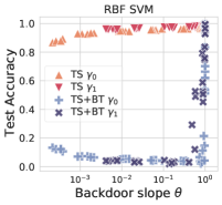
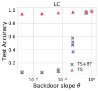
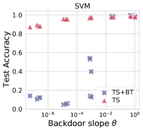
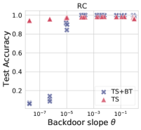
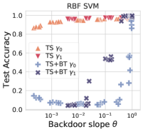
Figure 5: Backdoor slope $\theta$ vs clean accuracy (red) and backdoor effectiveness (blue) on MNIST 7 vs. 1 with backdoor trigger size $3\times 3$ (top row) and $6\times 6$ (bottom row). We measure the classification accuracy on the untainted test samples (TS), and on the same samples after adding the backdoor trigger (TS+BT). We chose the $\gamma$ parameter for the RBF kernel as $\gamma_{0}={5}\mathrm{e}{-04}$ (orange triangle for clean data, light blue plus for data with trigger) and $\gamma_{1}={5}\mathrm{e}{-03}$ (red inverted triangle for clean data, dark blue x for data with trigger).

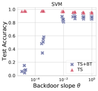
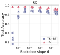
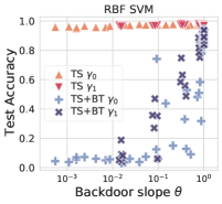
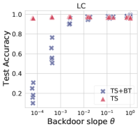
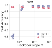
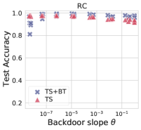
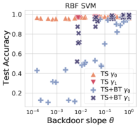
Figure 6: Backdoor slope $\theta$ vs clean accuracy (red) and backdoor effectiveness (blue) on CIFAR10 airplane vs frog with backdoor trigger size $8\times 8$ (top row), and $16\times 16$ (bottom row). We measure the classification accuracy on the untainted test samples (TS), and on the same samples after adding the backdoor trigger (TS+BT). We chose the $\gamma$ parameter for the RBF kernel as $\gamma_{0}={1}\mathrm{e}{-04}$ (orange triangle for clean data, light blue plus for data with trigger) and $\gamma_{1}={1}\mathrm{e}{-03}$ (red inverted triangle for clean data, dark blue x for data with trigger).

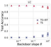
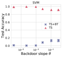
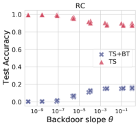
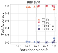
Figure 7: Backdoor slope $\theta$ vs clean accuracy (red) and backdoor effectiveness (blue) on Imagenette tench vs truck with trigger visibility $c_{m}=10$, i.e. almost imperceptible, (top row) and $c_{m}=75$ (bottom row). We measure the classification accuracy on the untainted test samples (TS), and on the same samples after adding the backdoor trigger (TS+BT). We chose the $\gamma$ parameter for the RBF kernel as $\gamma_{0}={1}\mathrm{e}{-05}$ (orange triangle for clean data, light blue plus for data with trigger) and $\gamma_{1}={1}\mathrm{e}{-04}$ (red inverted triangle for clean data, dark blue x for data with trigger).

Backdoor Slope. From the previous results we have seen that reducing complexity through regularization increases robustness against backdoors. For a deeper understanding of model complexity on backdoor learning, we leverage the proposed backdoor slope. In our experiments for convex-learners, we fix the fraction of injected poisoning points equal to $0.1$, as by Gu et al [1], and we report a dot for each combination of $\lambda$ and $\gamma$ as specified in Section 3.1. Figure 5-7 show the relationship between the backdoor slope and the backdoor effectiveness, measured as the percentage of samples with trigger that mislead the classifier, respectively for MNIST, CIFAR10 and Imagenette. We report the accuracy on the clean test dataset and on the test dataset with the backdoor trigger. For the SVM with RBF kernel, we report the accuracies for two different gamma.

Interestingly, our plots show a region where the accuracy of the classifier on benign samples is high, yet the classifier exhibits low accuracy on samples with trigger. For linear classifiers, this region equals low-regularized classifiers. In case of the RBF SVM, the best trade-off is achieved with high $\lambda$ (strong regularization) and small $\gamma$, which also constrain SVM’s complexity. Our results thus indicate that in these cases, the classifier is not flexible enough to learn the backdoor in addition to the clean test samples. Conversely, as long as the classifier has enough flexibility, it is able to learn the backdoor without sacrificing clean test accuracy. In a nutshell, choosing the hyperparameters appropriately, we can obtain a classifier able to learn the original task but not the backdoor. However, there is a trade-off between the accuracy on the original task and robustness to backdoor classification. In Figure 5-7 we further compare the relationship between backdoor learning slope and backdoor effectiveness considering a stronger attack (larger or more visible trigger). For these attacks, the trade-off region is reduced, leaving fewer possible configurations of the hyperparameters that yield a robust model. This result is consistent with our previous results using backdoor learning curves: the faster the curve descends when the trigger strength is increased, the higher the backdoor slope. Our results suggest that system designers should regularize models as much as possible while accepting a small accuracy loss in order to deploy a trustworthy ML algorithm.

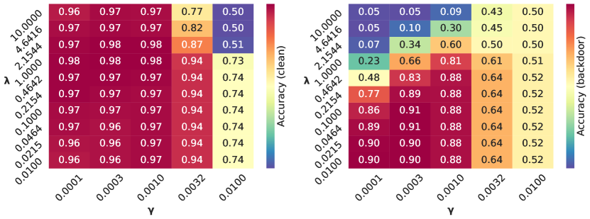
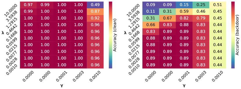
Figure 8: Influence of $\gamma$ (x-axis) and $\lambda$ (y-axis) on the backdoor effectiveness (left) and clean accuracy (right) for CIFAR10 airplane vs frog (top row) and Imagenette tench vs truck (bottom row). Backdoor is mounted with trigger size $8\times 8$ for CIFAR10 and visibility $c_{m}=75$ for Imagenette. The plots show that there are hyperparameter configurations for which clean accuracy is high (red regions on the left plots), while the accuracy on the backdoored points is low (blue regions on the right plots).

As a final check to asses the reliability of the backdoor learning slope, we plot in Figure 8 clean and backdoor accuracy when training an RBF SVM with different hyperparameter configurations. We train, for each configuration, the classifier on the poisoned dataset. On the top row we show the results for CIFAR10 airplane vs frog, and on bottom row the results for Imagenette tench vs truck. We followed the same backdoor setting for the backdoor slope in Figure 5-7, i.e. trigger size $8\times 8$ for MNIST and trigger visibility $c_{m}=75$ for Imagenette. Analogous to our previous findings, there exists a trade-off region where the clean accuracy is high (red), while the backdoor accuracy is low (blue), suggesting an higher robustness against backdoors. Analogous to the backdoor slope, the best region is obtained with reduced complexity, thus regularizing it or reducing $\gamma$. Although these matrices yield the same conclusion, it is worth to remark that computing the backdoor learning slope does not require to re-train the a specific classifier for each configuration on the poisoned training dataset. Therefore, backdoor learning slope can be used as tool for improving and speeding-up the hyperparameter optimization procedure, to look for accurate yet robust models.

Table 1: Backdoor learning slope for Resnet18 and Resnet50 when increasing the percentage of backdoor poisoning $p$, the number of epochs (#Epochs), and parameter $h$ for estimate in Eq. 7. We also report the corresponding backdoor effectiveness (Accuracy TS+BT) and clean accuracy (Accuracy TS+BT), measures respectively as the percentage correctly classified test samples with and without the backdoor trigger.

Model	$p$	#Epochs	Slope h=0.01	Slope h=0.1	Slope h=0.2	Slope h=1	Accuracy TS+BT	Accuracy TS
Resnet18	0.05	10	0.9955	0.9872	0.9752	0.9026	0.4163	0.9588
Resnet50	0.05	10	0.9965	0.9895	0.9785	0.9169	0.7197	0.9781
Resnet18	0.05	50	0.9986	0.9900	0.9797	0.9281	0.5256	0.9737
Resnet50	0.05	50	0.9992	0.9936	0.9849	0.9377	0.8067	0.9881
Resnet18	0.15	10	0.9955	0.9878	0.9774	0.9189	0.8804	0.9568
Resnet50	0.15	10	0.9966	0.9902	0.9943	0.9231	0.9440	0.9826
Resnet18	0.15	50	0.9987	0.9937	0.9864	0.9384	0.8893	0.9720
Resnet50	0.15	50	0.9992	0.9939	0.9971	0.9403	0.9509	0.9890

While this measure works well on convex learners, its roots in influence functions prevent a direct application on neural networks. As pointed out in [30] the analytical gradient in Eq. 5 at $\beta=0$ is unstable for DNNs. To overcome this deficiency we estimate it with finite difference approximation, obtaining:

$$\left.\frac{\partial L}{\partial\beta}\right|_{\beta=0}=\frac{L(\mathcal{P}_{\rm ts},\boldsymbol{w}^{\star}(h))-L(\mathcal{P}_{\rm ts},\boldsymbol{w}^{\star}(0))}{h}\,,$$ (7)

We report the the results for Resnet18 and Resnet50 in Table 1 where we used $h=\{0.01,0.1,0.2,1\}$. For each combination of poisoning percentage and number of epochs, we report the estimate of the backdoor learning slope when choosing different $h$ values. The closer $h$ is to $0$, the closer to $1$ is the backdoor slope of the neural network. This result is consistent with Figure 3, where the backdoor learning curves drop similarly fast, suggesting a high vulnerability of the model in the presence of backdoor samples. A subtle difference is that when increasing $h$, there is more evidence for higher vulnerability of neural networks trained with more epochs or when increasing the percentage of poisoning points.

In conclusion, after seen the results for convex-learners and neural networks, we state that a wise choice of the hyperaparameters, such as the regularization term $\lambda$, number of epochs or neurons, can allow the user to find a good tradeoff between accuracy on benign samples and robustness to backdoor poisoning.

Empirical Parameter Deviation Plots. After having investigated which factors influence backdoor effectiveness, we now focus our attention on how the model adapts/changes its parameters during the backdoor learning process, whether there is an increase in complexity or not.

We use our two measures proposed in Section 2, $\rho$ and $\nu$ to analyze the parameter change. The former, $\rho$, monitors the change of the weights, for example whether they increase or decrease. The latter, $\nu$, measures the change in orientation or angle of the classifier. We plot both measures with different regularization parameters, trigger size or visibility with fraction of poisoning points to $p=0.1$ in Figure 9-11.

On linear classifiers, $\rho(\boldsymbol{w})$ increases during the backdoor learning process. This equals an increase of the weights’ values, suggesting that the classifiers become more complex while learning the backdoor. However, when investigating the RBF SVM, the results are slightly different. Indeed, when increasing $\gamma$ and decreasing $\lambda$, the classifier becomes flexible and complex enough to learn the backdoor without increasing its complexity. On the other hand, when decreasing $\gamma$, the model is constrained to behave similarly to a linear classifier. In this way, analogously to linear classifiers, the model needs to increase its complexity to learn the backdoor. When increasing the trigger size or visibility the results are similar, thus confirming the previous analysis. However, as a results of increasing the attacker’s strength, the backdoor accuracy turns out to be higher.

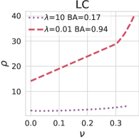
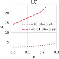
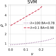
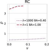
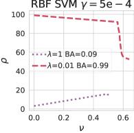
Figure 9: Backdoor weight deviation for the logistic classifier (LC), support vector machine (SVM), the ridge classifier (RC) and SVM with RBF kernel on MNIST $7~{}\rm{vs.}~{}1$ poisoned with backdoor trigger [1]. We report the results for trigger size $3\times 3$ (top row) and $6\times 6$ (bottom row). We specify regularization parameter $\lambda$ and backdoor accuracy (BA) for each setting in the legend of each plot.

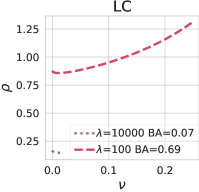
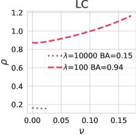
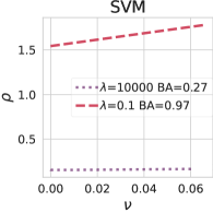
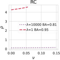
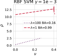
Figure 10: Backdoor weight deviation for the logistic classifier (LC), support vector machine (SVM), the ridge classifier (RC) and SVM with RBF kernel on CIFAR10 airplane vs frog poisoned with backdoor trigger [1]. We report the results for trigger size $8\times 8$ (top row) and $16\times 16$ (bottom row). We specify regularization parameter $\lambda$ and backdoor accuracy (BA) for each setting in the legend of each plot.

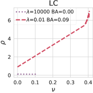
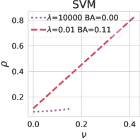
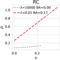
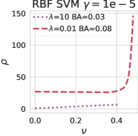
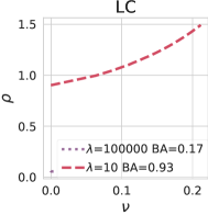
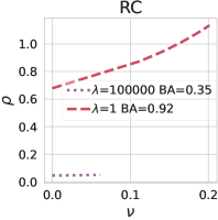
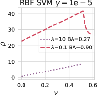
Figure 11: Backdoor weight deviation for the logistic classifier (LC), support vector machine (SVM), the ridge classifier (RC) and SVM with RBF kernel on Imagenette tench vs truck poisoned with backdoor trigger [28]. We report the results for visibility $c_{m}=10$ (top row) and $c_{m}=75$ (bottom row). We specify regularization parameter $\lambda$ and backdoor accuracy (BA) for each setting in the legend of each plot.

Explaining Backdoor Predictions. In the following, we give a graphical interpretation of the poisoned convex-classifier’s decision function, expressed by its internal weights, for which interpretation of their results is easier [24, 25]. We consider the results for backdoor trigger [1] in a specific position, as its influence on the classifier decision is easier to see. Conversely, the backdoor trigger by for example Zhong et al. [28] spans to the entire image, and therefore its influence is harder to spot from the interpretability plots. In particular, given a sample $x$ we aim to compute and show the gradient of the classifier’s decision function with respect to $x$. We use an SVM with regularization $\lambda={1}\mathrm{e}{-02}$ for MNIST $7~{}\rm{vs}~{}1$ and CIFAR10 airplane vs frog, and report the results in Figure 12. For MNIST we consider a digit $7$ with the trigger (left) and we show the gradient of the clean classifier’s decision function. We report the outcome of the gradient from the clean (middle) and poisoned (right) classifiers for the corresponding input. Since we train a linear classifier on the input space, the derivative coincide with the classifier’s weights. Intriguingly, the classifier’s weights increased their magnitude and now have high values on the bottom right corner, where the trigger is located. From CIFAR10, we show a poisoned airplane (left). We report the gradient mask obtained by considering the maximum value for each channel, both for the clean (middle) and backdoored (right) classifier. Also in this case, the backdoored model shows higher values in the bottom right region, corresponding to the trigger location. This means that the analyzed classifiers assign high importance to the trigger in order to discriminate the class of the input points.

Summarizing, the plots in Figure 12 further confirm our findings regarding the change of the internal parameters during the backdoor learning process. In particular, we have seen that less regularized classifiers need to increase their weights and thus complexity to learn the backdoor. Conversely, when the flexibility of the classifier increases then it can learn the backdoor easier without significantly altering its complexity.

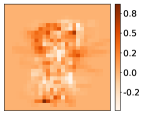
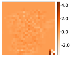
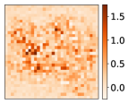
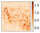
Figure 12: The first half of the plots consider the case of MNIST 7 vs. 1, and the second half is for CIFAR10 airplane vs frog. For each block we have: the poisoned test sample under consideration (left); the gradient of the untainted SVM decision’s boundary with respect to the input (middle); the gradient of the poisoned SVM decision’s boundary with respect to the input (right). For CIFAR10 we consider the maximum gradient of each pixel among the $3$ channels.

3.3 Visualizing Influential Training Points

Influence functions are used in the context of ML to identify the training points more responsible for a given prediction [10]. In Section 2 we have seen how they represent the basis of our backdoor learning slope measure. In this section, we employ them to show their outcomes and provide further insight into the relationship between complexity and backdoor effectiveness. To this end, as in Section 3.1, we poison $10\%$ of the training dataset. According with previous experiments, we employed the backdoor trigger in [1] for MNIST and CIFAR10 with trigger size $3\times 3$ and $6\times 6$ respectively, while for Imagenette we employed the trigger in Zhong et al. [28] with higher visibility (i.e. $c_{m}=75$). In Figure 13 and  14, considering respectively a high- and a low-complexity classifier, we report the seven most influential training samples on the classification of a randomly chosen test point. For high-complexity classifiers, many of these training samples contain the trigger. In contrast, this is not the case for low-complexity classifiers. These results suggest that low-complexity classifiers rely less on the samples containing the backdoor trigger in their predictions.

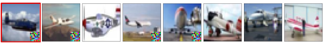
Figure 13: Influential training points for an high-complexity classifier. Considering an SVM with $\lambda=0.01$ trained on MNIST, and with $\lambda=0.1$ trained on CIFAR10, and Imagenette, we show the top $7$ most influential training samples on the prediction of the samples with the red border.

Figure 14: Influential training points for low-complexity classifiers. Considering an SVM with $\lambda=1e-3$ trained on MNIST, and with $\lambda=1e-5$ trained on CIFAR10, and Imagenette, we show the top $7$ most influential training samples on the prediction of the samples with the red border.

4 Related Work

We first review the literature about backdoor poisoning attacks and defenses. Afterwards, we focus on defenses that increase the robustness against backdoors by reducing the model’s complexity. We conclude the section by discussing the relationship between our proposed framework and influence functions.

Backdoor Poisoning. Although backdoors were introduced recently [1, 31], a plethora of backdoor attacks and defenses have already been published. For more detailed overview, we refer the reader to surveys in this area [32, 33]. Despite the quickly-growing literature about this topic, the majority of the previously proposed works [29, 34, 20] study different types of poisoning attacks, i.e., not backdoors. In contrast, only a few works have studied factors that influence the success of this attack. Baluta et al. [35] studied the relationship between backdoor effectiveness and the percentage of backdoored samples. Salem et al. [36] experimentally investigated the relationship between the backdoor effectiveness and the trigger size. We instead do not limit our study to neural networks but also study other models. Furthermore, we also investigate others relevant factors and the interaction between them.

Complexity and Backdoor Defenses. In this work, we have analyzed the relationship between backdoor effectiveness and different factors, including complexity, controlled via the regularization and the RBF kernel’s hyperparameter. Our experimental results show that reducing complexity by choosing appropriate hyperparameter values improves robustness against backdoors. Some of the defenses proposed against backdoors use different techniques to reduce complexity. These techniques include pruning [37, 38], data augmentation [39, 40] and gradient shaping [41]. However, from these works, it remains unclear why reducing complexity alleviates the threat of backdoor poisoning. To the best of our knowledge, our work is the first to investigate this aspect.

Relation to Influence Functions. Influence functions originated in robust statistics [42] and were later used as a tool to measure the influence of specific training points on the classification output [43, 10]. In our work, we clarify that influence functions naturally descend from the incremental learning formulation in Equation 1, showing that they quantify the velocity with which the classifier will learn new points. As seen in Section 2, they correspond to the partial derivative of the learning curve at the point $\beta=0$. Moreover, we leveraged them by proposing a measure, namely the backdoor slope, which quantifies the ability of a classifier to learn backdoors. This measure allowed us to study the factors that impact backdoor effectiveness.

5 Conclusions, Limitations and Future Work

In this paper, we presented a framework to analyze the factors influencing the effectiveness of backdoor poisoning. We carried out experiments on convex learners, also used in transfer-learning scenarios, and neural networks. As in previous work [10, 4], we focus our analysis on two-class classification problems for convex-learners, and on multiclass classification when considering neural networks. Our analysis shows that the effectiveness of backdoor attacks inherently depends on (i) the complexity of the target model, (ii) the fraction of backdoor samples in the training set, and (iii) the size and visibility of the backdoor trigger. By analyzing the influence of the first factor on backdoor learning, we are the first to unveil a region in the hyperparameter space where the accuracy on clean test samples is still high while the accuracy on backdoor samples is low. In particular, we found that the target model is required to significantly increase the complexity of its decision function to learn backdoors, which is impossible if the model is not flexible enough. Conversely, when decreasing the model’s complexity we can keep high performance on clean samples, and being unaffected by potential backdoor attacks. However, increasing the attacker’s strength, i.e. the last two factors, makes the attack more effective, shrinking this region and thus exposing the model to greater vulnerability. The study of more factors, like, for example, the dimensionality of the data, is straightforward using the proposed framework but left for future work. Our current results already provide important insights and provide a starting point to derive guidelines for designing models that are more robust against backdoor poisoning.

Appendix A Appendix

A.1 Additional Experimental Results

In the paper, we have shown the backdoor learning curves only for some classifiers. Here, we report them for all the classifiers considered in this work. As we will discuss later in this section, these results confirm the ones obtained in the paper. In particular, here we consider:

• Support Vector Machine (SVM) with $\lambda\in\{100,0.1\}$ for MNIST, $\lambda\in\{10000,0.1\}$ for CIFAR10, and $\lambda\in\{100000,1\}$ for Imagenette.

• Ridge Classifier (RC) with $\lambda\in\{1000,1\}$ for MNIST, $\lambda\in\{10000,1\}$ for CIFAR10, and $\lambda\in\{100000,1\}$ for Imagenette.

• Logistic Classifier (LC) with $\lambda\in\{10,0.01\}$ for MNIST, $\lambda\in\{10000,100\}$ for CIFAR10, and $\lambda\in\{100000,10\}$ for Imagenette.

• SVM with an RBF kernel, where $\lambda\in\{1,0.01\}$ and $\gamma={5}\mathrm{e}{-04}$ for MNIST, $\lambda\in\{100,1\}$ and $\gamma={1}\mathrm{e}{-03}$ for CIFAR10, and $\lambda\in\{10,0.1\}$ and $\gamma={1}\mathrm{e}{-05}$ for Imagenette.

Moreover, we compare the results obtained on the class pairs considered in the paper ($7~{}\rm{vs}~{}1$ on MNIST, airplane vs frog on CIFAR10 and Imagenette tench vs truck) with the ones obtained on different pairs.

Backdoor Learning Curves and Backdoor Learning Slope. In Figure 15-23 we report the backdoor learning curves for each classifier and dataset pair. In Figure 24-26, we report the backdoor learning slope, computed with $p=0.1$, for all the considered classifiers and all subset pairs. The results do not show significant variation with respect to the ones reported in the paper.

Empirical Parameter Deviation Plots. In Figure 27-29, shows how the classifiers’ parameters change when the classifiers learn the backdoors. This analysis is carried out with $p=0.1$. The results do not vary significantly across different classifiers and class pairs. The only exception is MNIST $5~{}\rm{vs}~{}2$. The untainted classifier is already quite complex; therefore, it does not increase its complexity when it learns the backdoor.

A.1.1 Increasing the trigger size or visibility

Although it is a known result in the literature that the size of the trigger increases the effectiveness of the attack [4, 36], here, for the first time to the best of our knowledge, we show how it interacts with other factors. In this section we report further experimental results when increasing the trigger size or visibility. As expected, the results in Fig. 30-31 show that choosing a larger trigger enhances the effectiveness of the attack. Indeed, when the trigger is larger or more visible the backdoor learning curves go down faster. Using the proposed backdoor slope to analyze the effect of complexity, controlled via the hyperparameters, on the vulnerability against backdoors, we found a region of the hyperparameter space that leads to having desirable performances: an accuracy high on the clean test samples and low on the ones containing the backdoor trigger.

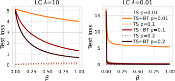
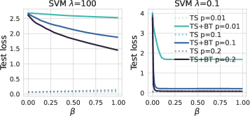
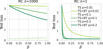
Figure 15: Backdoor learning curves for different classifiers trained on MNIST 7-1. Darker lines represent a higher fraction of poisoning samples $p$ injected into the training set. We report the loss on the clean test samples (TS) with a dashed line and on the test samples with the backdoor trigger (TS+BT) with a solid line.

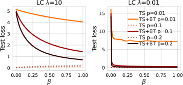
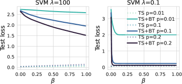
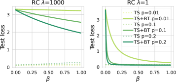
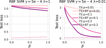
Figure 16: Backdoor learning curves for different classifiers trained on MNIST 3-0. See the caption of Figure 15 for further details.

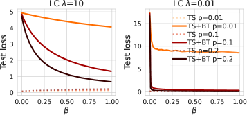
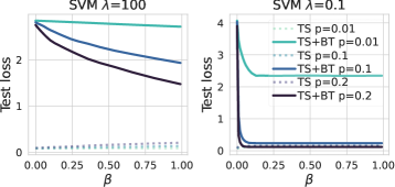
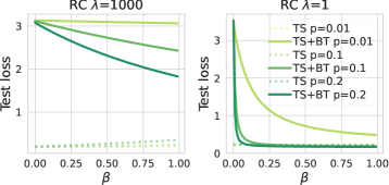
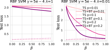
Figure 17: Backdoor learning curves for different classifiers trained on MNIST 5-2. See the caption of Figure 15 for further details.

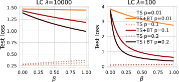
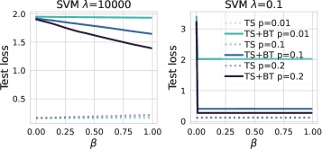
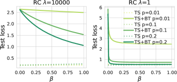
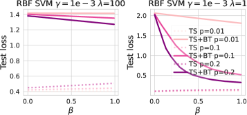
Figure 18: Backdoor learning curves for different classifiers trained on CIFAR10 airplane vs frog. See the caption of Figure 15 for further details.

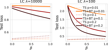
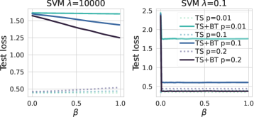
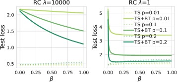
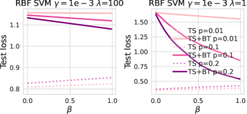
Figure 19: Backdoor learning curves for different classifiers trained on CIFAR10 bird vs dog. See the caption of Figure 15 for further details.

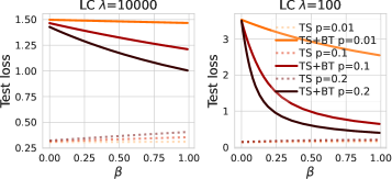
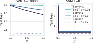
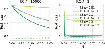
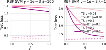
Figure 20: Backdoor learning curves for different classifiers trained on CIFAR10 airplane vs truck. See the caption of Figure 15 for further details.

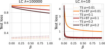
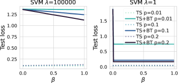
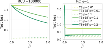
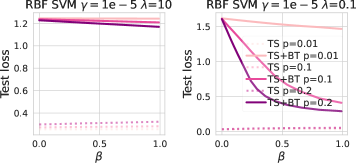
Figure 21: Backdoor learning curves for different classifiers trained on Imagenette tench vs truck. See the caption of Figure 15 for further details.

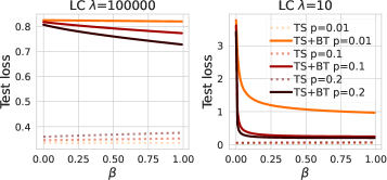
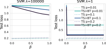
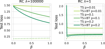
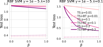
Figure 22: Backdoor learning curves for different classifiers trained on Imagenette cassette player vs church. See the caption of Figure 15 for further details.

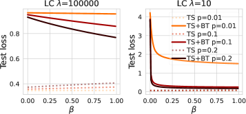
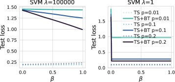
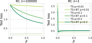
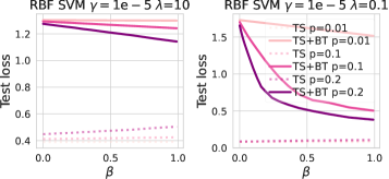
Figure 23: Backdoor learning curves for different classifiers trained on Imagenette tench vs parachute. See the caption of Figure 15 for further details.

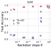
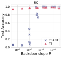
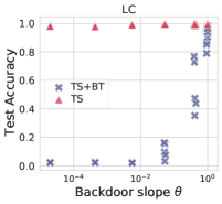
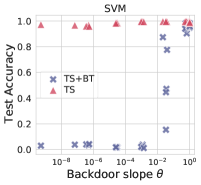
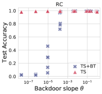
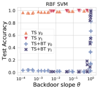
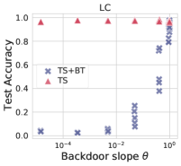
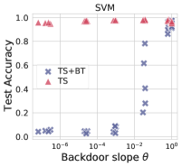
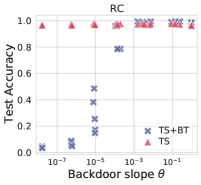
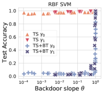
Figure 24: Backdoor slope $\theta$ vs clean accuracy (red) and backdoor effectiveness (blue) on MNIST 7vs.1 (top row), 3vs.0 (middle row) and 5vs.2 (bottom row). We measure the classification accuracy on the untainted test samples (TS), and on the same samples after adding the $3\times 3$ backdoor trigger (TS+BT). We chose the $\gamma$ parameter for the RBF kernel as $\gamma_{0}={5}\mathrm{e}{-04}$ (orange triangle for clean data, light blue plus for data with trigger) and $\gamma_{1}={5}\mathrm{e}{-03}$ (red inverted triangle for clean data, dark blue x for data with trigger).

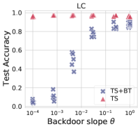
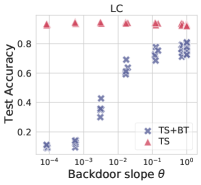
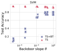
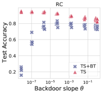
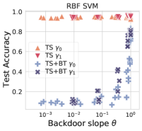
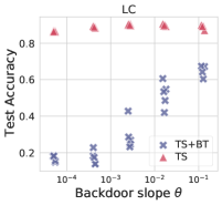
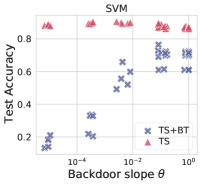
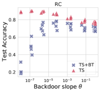
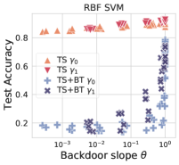
Figure 25: Backdoor slope vs backdoor (BK) effectiveness on CIFAR10 airplane vs frog (top row), airplane vs truck (middle row) and bird vs dog (bottom row). See the caption of Figure 24 for further details. The results are obtained considering a trigger size equal to $8$.

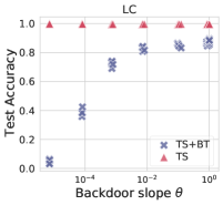
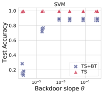
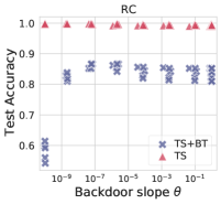
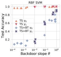
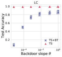
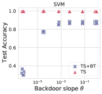
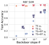
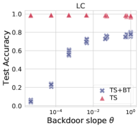
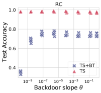
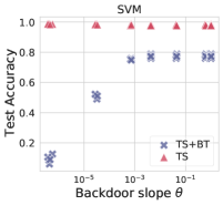
Figure 26: Backdoor slope vs backdoor (BK) effectiveness on Imagenette tench vs truck (top row), cassette player vs church (middle row) and tench vs parachute (bottom row). See the caption of Figure 24 for further details. The results are obtained considering a trigger size equal to $8$.

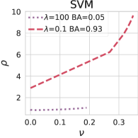
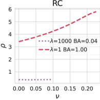
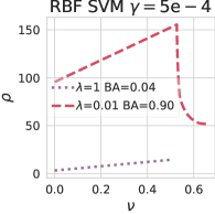
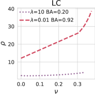
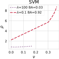
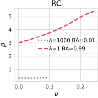
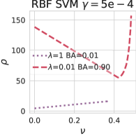
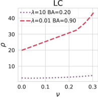
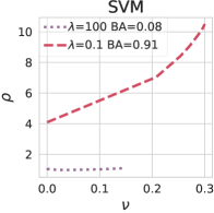
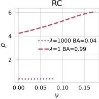
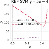
Figure 27: Backdoor weight deviation for different classifiers trained on MNIST $7~{}\rm{vs}~{}1$ (top row), $3~{}\rm{vs}~{}0$ (middle row) and $5~{}\rm{vs}~{}2$ (bottom row). We specify regularization parameter $\lambda$ and backdoor (BK) accuracy for each setting in the legend of each plot.

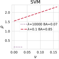
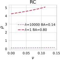
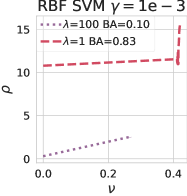
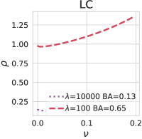
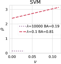
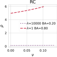
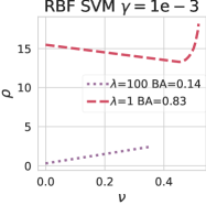
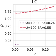
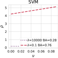
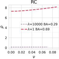
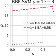
Figure 28: Backdoor weight deviation for different classifiers trained on CIFAR10 airplane vs frog (top), airplane vs truck (middle), and bird vs dog (bottom). See Figure 27 for further details.

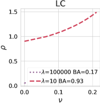
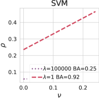
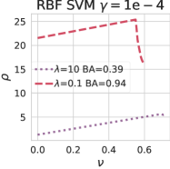
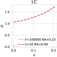
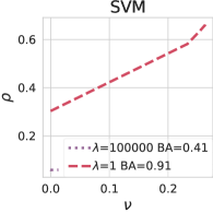
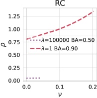
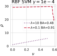
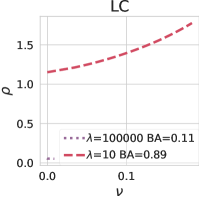
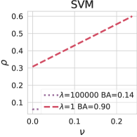
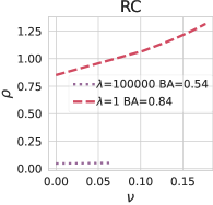
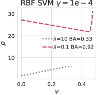
Figure 29: Backdoor weight deviation for different classifiers trained on Imagenette tench vs truck (top), tench vs parachute (middle), and cassette player vs church (bottom). See Figure 27 for further details.

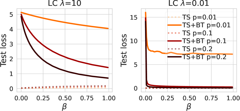
(a) MNIST trigger size $3\times 3$.

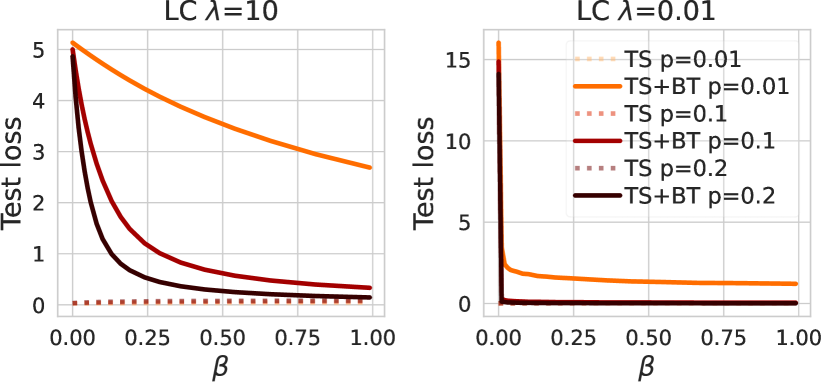
(b) MNIST trigger size $6\times 6$.

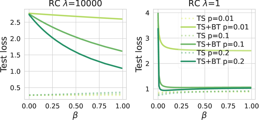
(c) CIFAR10 trigger size $8\times 8$.

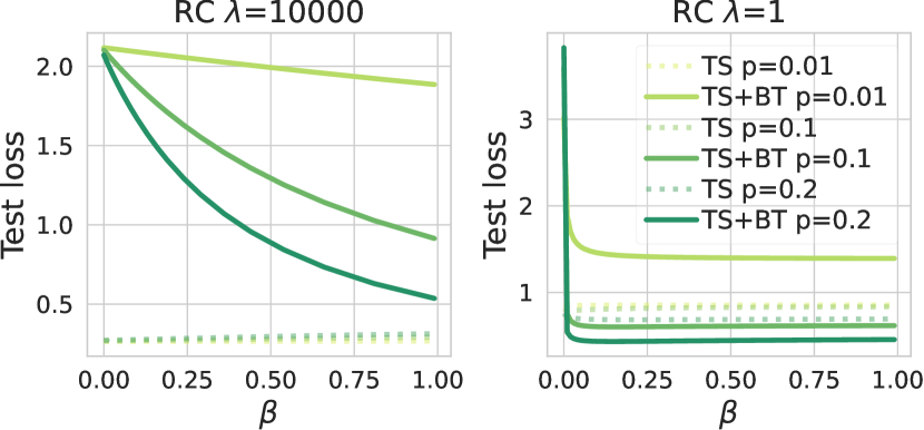
(d) CIFAR10 trigger size $16\times 16$.

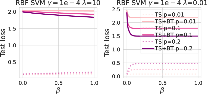
(e) Imagenette trigger visibility $c_{m}=10$.

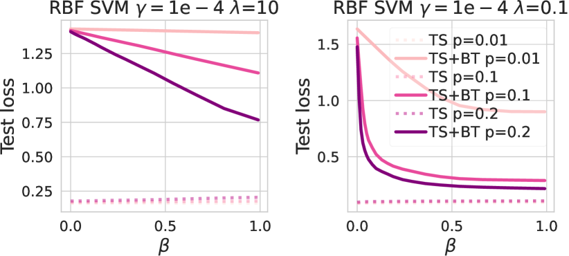
(f) Imagenette trigger visibility $c_{m}=75$.

Figure 30: Backdoor learning curves for: (top row) LC on MNIST 3vs.0 with trigger size 3$\times$3 (left) or 6$\times$6 (right); (middle row) RC on CIFAR10 airplane vs truck with trigger size 8$\times$8 (left) or 16$\times$16 (right); (bottom row) RBF SVM on Imagenette cassette player vs church with trigger visibility $c_{m}$=10 (left) or $c_{m}$=75 (right). Further details in Figure 15.

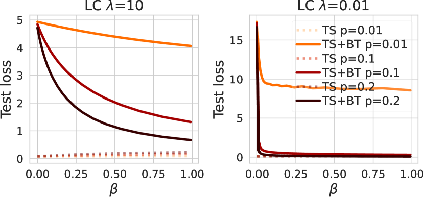
(a) MNIST trigger size $3\times 3$.

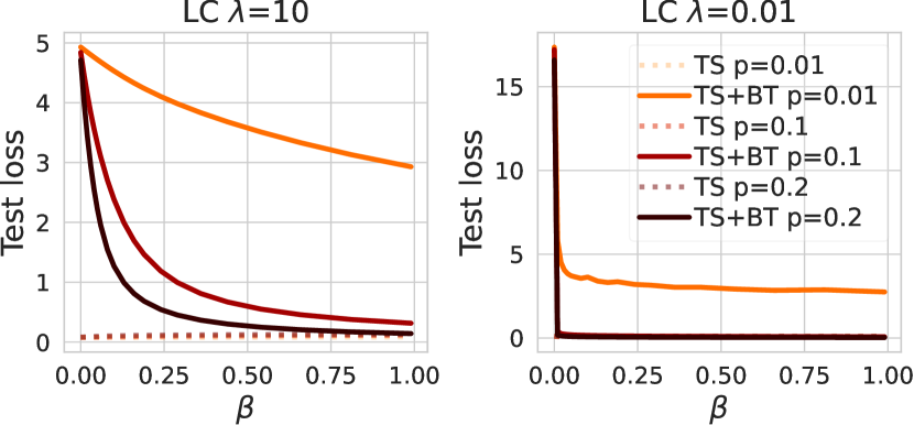
(b) MNIST trigger size $6\times 6$.

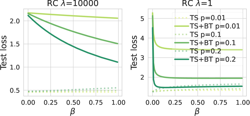
(c) CIFAR10 trigger size $8\times 8$.

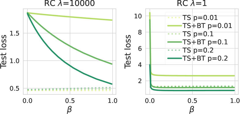
(d) CIFAR10 trigger size $16\times 16$.

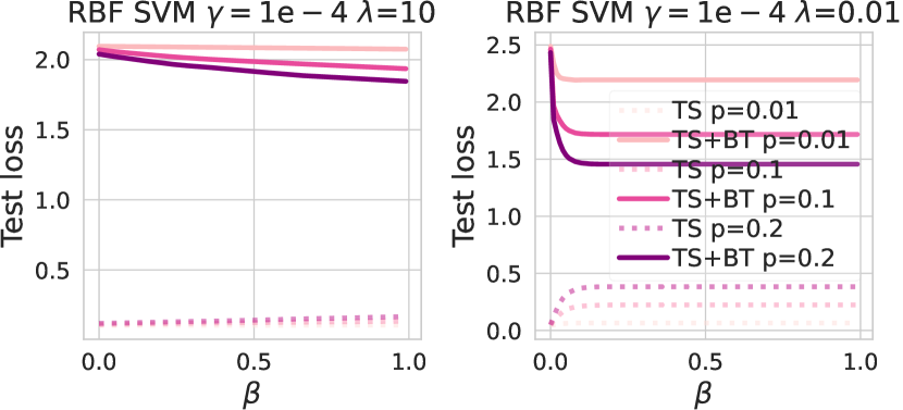
(e) Imagenette trigger visibility $c_{m}=10$.

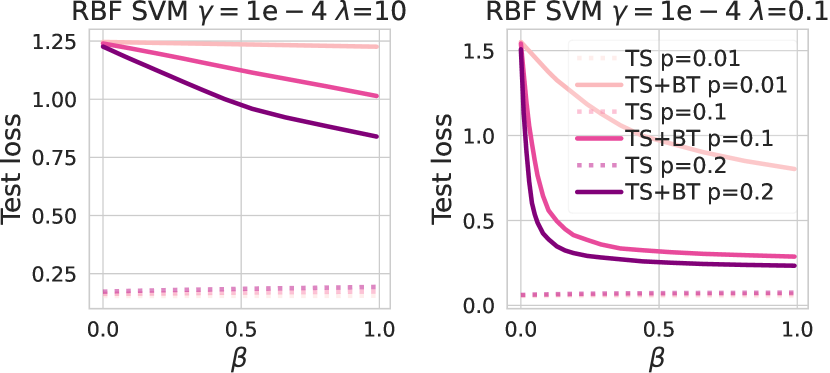
(f) Imagenette trigger visibility $c_{m}=75$.

Figure 31: Backdoor learning curves for: (top row) LC on MNIST 5 vs. 2; (middle row) RC on CIFAR10 bird vs dog; (bottom row) RBF SVM on Imagenette tench vs parachute.

References

- [1] Tianyu Gu, Kang Liu, Brendan Dolan-Gavitt, and Siddharth Garg. Badnets: Evaluating backdooring attacks on deep neural networks. IEEE Access, 7:47230–47244, 2019.
- [2] Yingqi Liu, Shiqing Ma, Yousra Aafer, Wen-Chuan Lee, Juan Zhai, Weihang Wang, and Xiangyu Zhang. Trojaning attack on neural networks. In NDSS, 2018.
- [3] Xinyun Chen, Chang Liu, Bo Li, Kimberly Lu, and D. Song. Targeted backdoor attacks on deep learning systems using data poisoning. ArXiv, abs/1712.05526, 2017.
- [4] Aniruddha Saha, Akshayvarun Subramanya, and Hamed Pirsiavash. Hidden trigger backdoor attacks. In The Thirty-Fourth AAAI Conference on Artificial Intelligence, AAAI 2020, The Thirty-Second Innovative Applications of Artificial Intelligence Conference, IAAI 2020, The Tenth AAAI Symposium on Educational Advances in Artificial Intelligence, EAAI 2020, New York, NY, USA, February 7-12, 2020, pages 11957–11965, 2020.
- [5] Xiaoyi Chen, Ahmed Salem, Michael Backes, Shiqing Ma, and Yang Zhang. Badnl: Backdoor attacks against nlp models. arXiv:2006.01043, 2020.
- [6] Zhaohan Xi, Ren Pang, Shouling Ji, and Ting Wang. Graph backdoor. In 30th USENIX Security Symposium (USENIX Security 21), 2021.
- [7] Panagiota Kiourti, Kacper Wardega, Susmit Jha, and Wenchao Li. Trojdrl: evaluation of backdoor attacks on deep reinforcement learning. In 2020 57th ACM/IEEE Design Automation Conference (DAC), pages 1–6. IEEE, 2020.
- [8] Gert Cauwenberghs and Tomaso Poggio. Incremental and decremental support vector machine learning. Advances in neural information processing systems, pages 409–415, 2001.
- [9] Trevor Hastie, Saharon Rosset, Robert Tibshirani, and Ji Zhu. The entire regularization path for the support vector machine. J. Mach. Learn. Res., 5:1391–1415, 2004.
- [10] Pang Wei Koh and Percy Liang. Understanding black-box predictions via influence functions. In ICML, 2017.
- [11] Jonathan Lorraine, Paul Vicol, and David Duvenaud. Optimizing millions of hyperparameters by implicit differentiation. In Silvia Chiappa and Roberto Calandra, editors, Proceedings of the Twenty Third Int. Conference on Artificial Intelligence and Statistics, volume 108 of Proceedings of Machine Learning Research, pages 1540–1552, 26–28 Aug 2020.
- [12] Luca Franceschi, Paolo Frasconi, Saverio Salzo, Riccardo Grazzi, and Massimiliano Pontil. Bilevel programming for hyperparameter optimization and meta-learning. In Jennifer Dy and Andreas Krause, editors, 35th ICML, volume 80 of Proc. Mach. Learn. Res., pages 1568–1577, 2018.
- [13] F. Pedregosa. Hyperparameter optimization with approximate gradient. In Maria Florina Balcan and Kilian Q. Weinberger, editors, 33rd Int. Conference on Machine Learning, volume 48 of Proceedings of Machine Learning Research, pages 737–746, New York, New York, USA, 20–22 Jun 2016. PMLR.
- [14] Dougal Maclaurin, David Duvenaud, and Ryan P. Adams. Gradient-based hyperparameter optimization through reversible learning. In Proceedings of the 32Nd Int. Conference on Int. Conference on Machine Learning - Volume 37, ICML’15, pages 2113–2122, 2015.
- [15] Justin Domke. Generic methods for optimization-based modeling. In Neil D. Lawrence and Mark Girolami, editors, 15th Int’l Conf. Artificial Intelligence and Statistics, volume 22 of Proceedings of Machine Learning Research, pages 318–326, La Palma, Canary Islands, 21–23 Apr 2012. PMLR.
- [16] Chiyuan Zhang, Samy Bengio, and Yoram Singer. Are all layers created equal? CoRR, abs/1902.01996, 2019.
- [17] Yann LeCun, Corinna Cortes, and CJ Burges. Mnist handwritten digit database. ATT Labs [Online]. Available: http://yann.lecun.com/exdb/mnist, 2, 2010.
- [18] Alex Krizhevsky. Learning multiple layers of features from tiny images. Technical report, 2009.
- [19] Jeremy Howard. imagenette.
- [20] Fnu Suya, Saeed Mahloujifar, Anshuman Suri, David Evans, and Yuan Tian. Model-targeted poisoning attacks with provable convergence. In Int. Conference on Machine Learning, pages 10000–10010. PMLR, 2021.
- [21] Jeff Donahue, Y. Jia, Oriol Vinyals, Judy Hoffman, Ning Zhang, Eric Tzeng, and Trevor Darrell. Decaf: A deep convolutional activation feature for generic visual recognition. In ICML, 2014.
- [22] Giulia Pasquale, Carlo Ciliberto, Francesca Odone, Lorenzo Rosasco, and Lorenzo Natale. Teaching icub to recognize objects using deep convolutional neural networks. In Proceedings of the 4th Workshop on Machine Learning for Interactive Systems, MLIS 2015, co-located with the 32nd Int. Conference on Machine Learning (ICML 2015), Lille, France, July 11th, 2015, volume 43 of JMLR Workshop and Conference Proceedings, pages 21–25, 2015.
- [23] A. Krizhevsky, Ilya Sutskever, and Geoffrey E. Hinton. Imagenet classification with deep convolutional neural networks. volume 60, pages 84 – 90, 2012.
- [24] Florian Tramèr and Dan Boneh. Differentially private learning needs better features (or much more data). In 9th Int. Conference on Learning Representations, ICLR 2021, Virtual Event, Austria, May 3-7, 2021, 2021.
- [25] Maurizio Ferrari Dacrema, P. Cremonesi, and D. Jannach. Are we really making much progress? a worrying analysis of recent neural recommendation approaches. 2019.
- [26] Pankaj Mehta, M. Bukov, Ching-Hao Wang, A. G. Day, C. Richardson, Charles K. Fisher, and D. Schwab. A high-bias, low-variance introduction to machine learning for physicists. Physics reports, 810:1–124, 2019.
- [27] Rich Caruana, Steve Lawrence, and C. Lee Giles. Overfitting in neural nets: Backpropagation, conjugate gradient, and early stopping. In Todd K. Leen, Thomas G. Dietterich, and Volker Tresp, editors, Advances in Neural Information Processing Systems 13, Papers from Neural Information Processing Systems (NIPS) 2000, Denver, CO, USA, pages 402–408, 2000.
- [28] Haoti Zhong, Cong Liao, Anna Cinzia Squicciarini, Sencun Zhu, and David J. Miller. Backdoor embedding in convolutional neural network models via invisible perturbation. In Vassil Roussev, Bhavani M. Thuraisingham, Barbara Carminati, and Murat Kantarcioglu, editors, CODASPY ’20: Tenth ACM Conference on Data and Application Security and Privacy, New Orleans, LA, USA, March 16-18, 2020, pages 97–108, 2020.
- [29] Christopher Frederickson, Michael Moore, Glenn Dawson, and Robi Polikar. Attack strength vs. detectability dilemma in adversarial machine learning. In 2018 Int. Joint Conference on Neural Networks (IJCNN), pages 1–8. IEEE, 2018.
- [30] Samyadeep Basu, Philip Pope, and Soheil Feizi. Influence functions in deep learning are fragile. In ICLR, 2021.
- [31] Xinyun Chen, Chang Liu, Bo Li, Kimberly Lu, and Dawn Song. Targeted backdoor attacks on deep learning systems using data poisoning. arXiv:1712.05526, 2017.
- [32] Yansong Gao, Bao Gia Doan, Zhi Zhang, Siqi Ma, Jiliang Zhang, Anmin Fu, Surya Nepal, and Hyoungshick Kim. Backdoor attacks and countermeasures on deep learning: A comprehensive review. CoRR, abs/2007.10760, 2020.
- [33] Micah Goldblum, Dimitris Tsipras, Chulin Xie, Xinyun Chen, Avi Schwarzschild, Dawn Song, Aleksander Madry, Bo Li, and Tom Goldstein. Data security for machine learning: Data poisoning, backdoor attacks, and defenses. arXiv:2012.10544, 2020.
- [34] Javier Carnerero-Cano, Luis Munoz-González, Phillippa Spencer, and Emil C Lupu. Regularization can help mitigate poisoning attacks… with the right hyperparameters. In ICLR Workshop on Security and Safety in Machine Learning System, 2021.
- [35] Teodora Baluta, Shiqi Shen, Shweta Shinde, Kuldeep S Meel, and Prateek Saxena. Quantitative verification of neural networks and its security applications. In CCS, 2019.
- [36] Ahmed Salem, Rui Wen, Michael Backes, Shiqing Ma, and Yang Zhang. Dynamic backdoor attacks against machine learning models. CoRR, abs/2003.03675, 2020.
- [37] Kang Liu, Brendan Dolan-Gavitt, and Siddharth Garg. Fine-pruning: Defending against backdooring attacks on deep neural networks. In Int. Symposium on Research in Attacks, Intrusions, and Defenses, pages 273–294. Springer, 2018.
- [38] Peter Bajcsy and Michael Majurski. Baseline pruning-based approach to trojan detection in neural networks. arXiv:2101.12016, 2021.
- [39] Yi Zeng, Han Qiu, Shangwei Guo, Tianwei Zhang, Meikang Qiu, and Bhavani Thuraisingham. Deepsweep: An evaluation framework for mitigating dnn backdoor attacks using data augmentation. arXiv:2012.07006, 2020.
- [40] Eitan Borgnia, Valeriia Cherepanova, Liam Fowl, Amin Ghiasi, Jonas Geiping, Micah Goldblum, Tom Goldstein, and Arjun Gupta. Strong data augmentation sanitizes poisoning and backdoor attacks without an accuracy tradeoff. In ICASSP 2021-2021 IEEE Int. Conference on Acoustics, Speech and Signal Processing (ICASSP), pages 3855–3859. IEEE, 2021.
- [41] Sanghyun Hong, Varun Chandrasekaran, Yiğitcan Kaya, Tudor Dumitraş, and Nicolas Papernot. On the effectiveness of mitigating data poisoning attacks with gradient shaping. arXiv:2002.11497, 2020.
- [42] R Dennis Cook and Sanford Weisberg. Characterizations of an empirical influence function for detecting influential cases in regression. Technometrics, 22(4):495–508, 1980.
- [43] Andreas Christmann and Ingo Steinwart. On robustness properties of convex risk minimization methods for pattern recognition. The Journal of Machine Learning Research, 5:1007–1034, 2004.