Examining and Combating Spurious Features under Distribution Shift

Abstract

A central goal of machine learning is to learn robust representations that capture the causal relationship between inputs features and output labels. However, minimizing empirical risk over finite or biased datasets often results in models latching on to spurious correlations between the training input/output pairs that are not fundamental to the problem at hand. In this paper, we define and analyze robust and spurious representations using the information-theoretic concept of minimal sufficient statistics. We prove that even when there is only bias of the input distribution (i.e. covariate shift), models can still pick up spurious features from their training data. Group distributionally robust optimization (DRO) provides an effective tool to alleviate covariate shift by minimizing the worst-case training loss over a set of pre-defined groups. Inspired by our analysis, we demonstrate that group DRO can fail when groups do not directly account for various spurious correlations that occur in the data. To address this, we further propose to minimize the worst-case losses over a more flexible set of distributions that are defined on the joint distribution of groups and instances, instead of treating each group as a whole at optimization time. Through extensive experiments on one image and two language tasks, we show that our model is significantly more robust than comparable baselines under various partitions. Our code is available at https://github.com/violet-zct/group-conditional-DRO.

1 Introduction

Many machine learning models that minimize the average training loss via empirical risk minimization (ERM) are trained and evaluated on randomly shuffled and split training and test sets. However, such in-distribution learning setups can hide critical issues: models that achieve high accuracy on average often underperform when the test distribution drifts away from the training one (Hashimoto et al., 2018; Koenecke et al., 2020; Koh et al., 2020). Such models are often “right for the wrong reasons” due to reliance on spurious correlations (or “dataset biases”) (Torralba & Efros, 2011; Goyal et al., 2017; McCoy et al., 2019; Gururangan et al., 2018), heuristics that hold for most training examples but are not inherent to the task of interest, such as strong associations between the presence of green pastures background with the label “cows” in image classification. Naturally, models that use such features will fail when tested on data where the correlation does not hold.

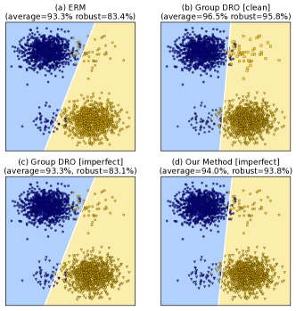
Figure 1: Consider data points $x$ in $\mathbb{R}^{2}$ with two classes $y$. The vertical axis of $x$ is a spurious feature that highly correlates with $y$, and the horizontal axis is the robust feature. There are two subclasses in each class, where the top-right and lower-left are two minority subclasses. The robust accuracy is test worst-case accuracy over the four subclasses. We train a linear classifier with different methods. For models trained with the clean partitions, each subclass is a group. For the imperfect partitions, dots with the same shape is a group (best viewed in color).

Recent work has investigated how models trained with ERM learn spurious features that do not generalize, from the points of view of causality (Arjovsky et al., 2019), understanding model overparameterization (Sagawa et al., 2020b) and information theory (Lovering et al., 2021). However, these works have not characterized the idea of spurious features mathematically. In this paper, we characterize spurious features from an information-theoretic perspective. We consider prediction of target random variable $Y\in\mathcal{Y}$ from input variable $X\in\mathcal{X}$ and characterize spurious features learned under changes to the input distribution $p(X)$ (i.e. covariate shift).

A central goal of machine learning is to learn true causal relationships between $X$ and $Y$ in a manner robust to spurious factors concerning the variables. We assume that there exists an “ideal” data distribution $p_{\text{ideal}}$ (short for $p_{\text{ideal}}(X,Y)$ below) which contains data from all possible experimental conditions concerning the confounders that cause spurious correlations, both observable and hypothetical (Lewis, 2013; Arjovsky et al., 2019; Bellot & van der Schaar, 2020). For example, consider the problem of classifying images of cows and camels (Beery et al., 2018). Under the ideal conditions, we assume that pictures of cows and camels on any background can be collected, including cows in deserts and camels in green pastures. Therefore, under $p_{\text{ideal}}$ the background of the image $X$ is no longer a spurious factor of the label $Y$. However, such an “ideal” distribution $p_{\text{ideal}}$ is not accessible in practice (Bahng et al., 2020; Koh et al., 2020; McCoy et al., 2019), and our training distribution $p_{\text{train}}$ (often, in practice, an associated empirical distribution) does not match $p_{\text{ideal}}$. ERM-based learning algorithms indiscriminately fit all correlations found in $p_{\text{train}}$, including spurious correlations based on confounders (Tenenbaum, 2018; Lopez-Paz, 2016).

To investigate the spurious features learned under the distribution shift from $p_{\text{ideal}}$ to $p_{\text{train}}$, we first characterize those features of $X$ which most efficiently capture all possible information needed to predict $Y$. We define these robust features using the notion of minimal sufficient statistic (MSS) (Dynkin, 2000; Cvitkovic & Koliander, 2019) under $p_{\text{ideal}}$. We then examine whether the features learned under $p_{\text{train}}$ contain spurious features compared to the MSS learned under $p_{\text{ideal}}$. Through our analysis, we find that even only with covariate shift, the features learned on $p_{\text{train}}$ can contain spurious features or miss robust features of $p_{\text{ideal}}$.

Models that fit spurious correlations in $p_{\text{train}}$ can be vulnerable to groups (subpopulations of $p_{\text{ideal}}$/$p_{\text{test}}$) where the correlation does not hold. A common approach to avoid learning a model that suffers high worst group errors is group distributionally robust optimization (group DRO), a training procedure that efficiently minimizes the worst expected loss over a set of groups in the training data (Oren et al., 2019; Sagawa et al., 2020a). The partition of groups can be defined in several ways, such as by presence of manually identified potentially spurious features (Sagawa et al., 2020a), data domains (Koh et al., 2020), or topics of text (Oren et al., 2019). In a typical setup, the groups of interest in the test set align with those used to partition the training data. Under such setups, group DRO usually outperforms ERM with respect to the worst-group accuracy. We contend that this is because it promotes learning robust features that perform uniformly well across all groups. However, in many tasks, we can not collect clean group membership of training examples due to expensive annotation cost or privacy concerns regarding e.g. demographic identities of users or other sensitive information.

Inspired by our analysis of spurious features, we demonstrate that group DRO can fail under “imperfect” partitions of training data that are not consistent with the test set, especially when reducing spurious correlation in one group could exacerbate the spurious correlations in another (§4.2), as shown in Fig. 1. This is because group DRO treats each training group as a unit, preventing it from adjusting learning weights differently for subgroups within each group. Recent work has proposed to use sophisticated unsupervised clustering algorithm to search for meaningful subclasses (Sohoni et al., 2020) and execute group DRO on the found subclasses. To learn robust models under noisy protected groups, Wang et al. (2020) designs robust approaches that is based on an estimate of a noise model between the clean and noisy groups. Instead of relying on good partitions of groups or a not readily available noise model, we propose group-conditional DRO (GC-DRO) that defines the uncertainty set over the joint distribution of groups and their instances (i.e. $q(G)q(X,Y|G)$). Every training example is reweighted by both its group weight and the instance-level weight, which offers a more flexible uncertainty set compared to group DRO. Through extensive experiments on three tasks — facial attribute classification, natural language inference, and toxicity detection, we show that GC-DRO significantly outperforms both ERM and group DRO in various partitions of training data and demonstrate the robustness of GC-DRO against various group partitions.

2 Preliminaries on Robust Representations

To study spurious features, we need to formally define which features or properties of the data describe spurious correlations, and which features are robust features relevant to the task at hand. In supervised learning we are interested in finding a good representation $T(X)$ of the input $X$ that is useful to predict a target label $Y$. What characterizes the optimal representations of $X$ w.r.t. $Y$ is much debated, but a common assertion is that $T(X)$ should be a minimal sufficient statistic (MSS) of $X$ for $Y$ (Adragni & Cook, 2009; Schwartz-Ziv & Tishby, 2017; Achille & Soatto, 2018; Cvitkovic & Koliander, 2019), which is:

(i) $T(X)$ should be sufficient for $Y$, i.e. $\forall x\in\mathcal{X},t\in\mathcal{T},y\in\mathcal{Y},p(x|t,y)=p(x|t)$, which is equivalent to $p(y|t,x)=p(y|t)$. This means given the value of $T(X)$, the distribution of $X$ does not depend on the value of $Y$.

(ii) Given that $T(X)$ is sufficient, it should be minimal w.r.t. $X$, i.e. for any sufficient statistic $S$, there exists a deterministic function $f$ such that $T=f(S)$ almost everywhere w.r.t. $X$. This means for any measurable, non-invertible function $g$, $g(T)$ is no longer sufficient for $Y$.

In other words, the minimal sufficient statistics most efficiently capture all information useful for predicting $Y$. The notion of MSS has been connected to Shannon’s information theory (Kullback & Leibler, 1951; Cover, 1999) and extended to any joint distribution $P(X,Y)$ of $X$ and $Y$ in the information bottleneck (IB) framework (Tishby et al., 2000; Shamir et al., 2010; Kolchinsky et al., 2019), which provides a principled way to characterize the extraction of relevant information from $X$ for predicting $Y$. Loosely speaking, learning a MSS $T$ is equivalent to maximizing $I(T(X);Y)$ (sufficiency) and minimizing $I(X;T(X))$ (minimality).

Robust Features. Suppose $\mathcal{A}$ contains all possible combinations of spurious variables, both observable and hypothetical, and we consider datasets $\mathcal{D}_{(a,y)}=\{x_{i}\}_{i=1}^{N_{a,y}}$ collected under each condition of $(a\in\mathcal{A},y\in\mathcal{Y})$, where each $\mathcal{D}_{(a,y)}$ contains examples that are i.i.d. according to some probability distribution $p(X|y,a)$. We define $p_{\text{ideal}}$ as the mixture distribution of $p(X|y,a)$ with uniform weights over $(a,y)\in\mathcal{A}\times\mathcal{Y}$. Thus, MSS learned on $p_{\text{ideal}}$ provide a good candidate for robust features $T(X)$ (sometimes denoted $T_{ideal}(X)$ for clarity), which most efficiently capture the information from $X$ necessary for predicting $Y$ on a distribution that is free of spurious factors.

Spurious Features. In contrast, we define representations $T^{\prime}(X)$ that contain spurious features. Specifically, the entropy of $T^{\prime}(X)$ conditioned on $T(X)$ under $p_{\text{ideal}}$ is positive.

$$\small H_{{\color[rgb]{0,0,1}ideal}}(T^{\prime}(X)|T(X))>0\vspace{-1mm}$$ (1)

Because these learned features are not deterministic given $T(X)$ then they contain additional information that is not useful for predicting $Y$. For example, in image classification, knowing that the image contains a horse, we cannot predict the background with certainty (a horse could be on a race track or a beach). Another example in natural language inference (NLI) task is that model learned on a biased data set often associates negation with the label “contradiction”. This is another spurious feature under our definition, because given the meaning of a sentence (robust features), whether it contains negation or not is not deterministic, e.g. “Don’t worry.” and “Be calm.” are synonymous but only one contains negation. A classifier that uses these spurious features can suffer from the risk of learning the spurious correlations between $T^{\prime}(X)$ and the labels $Y$.

3 Spurious Features under Covariate Shift

The training data is often marred by various abnormalities, such as selection biases (Buolamwini & Gebru, 2018) and confounding factors (Gururangan et al., 2018). We ask if the MSS learned under $p_{\text{train}}$ are robust features under $p_{\text{ideal}}$. Note that we do not study how to learn MSS via ERM in this paper, on the other hand, considering that MSS provides a good candidate for robust representations, we want to study if the MSS learned under $p_{\text{train}}$ contains spurious features with respect to the MSS learned under $p_{\text{ideal}}$, which are universal robust features against various spurious factors.

We consider the distribution shift in $p(X)$, also known as covariate shift (David et al., 2010), and we show that the entropy of MSS learned under $p_{\text{train}}$ conditioned on the robust features is zero in Theorem 1 with proofs in §A.

Theorem 1.

Suppose that there is only covariate shift in $p_{\text{train}}$, i.e. $\exists x\in\mathcal{X}_{train}\text{~{}s.t.~{}}p_{\text{train}}(x)\neq p_{\text{ideal}}(x)$ but $p_{\text{train}}(Y|X=x)=p_{\text{ideal}}(Y|X=x),\,\,\forall x\in\mathcal{X}_{train}$. Let $T_{\text{train}}(X)$ be the MSS representation learned under $p_{\text{train}}$, then we have:

$$\small H_{{\color[rgb]{0,0,1}train}}(T_{train}(x)|T_{ideal}(x))=0.\vspace{-2mm}$$ (2)

Theorem 1 tells us that $T_{train}(X)$ is deterministic given $T_{ideal}(X)$ under ${\color[rgb]{0,0,1}p_{\text{train}}}$ (shown in blue to distinguish from Eq. 1). However, this does not imply $H_{ideal}(T_{train}(X)|T_{ideal}(X))=0$ under ${\color[rgb]{0,0,1}p_{\text{ideal}}}$. Thus, we cannot conclude that $T_{train}(X)$ contains no spurious features. We further discuss the implications with two cases based on the relationship between the support of input $\mathcal{X}_{train}$ and that of $\mathcal{X}_{ideal}$: (1) $\mathcal{X}_{train}=\mathcal{X}_{ideal}$ and (2) $\mathcal{X}_{train}\subset\mathcal{X}_{ideal}$. When the input support of $p_{\text{train}}$ is equal to that of $p_{\text{ideal}}$, we have the following corollary:

Corollary 1.

Suppose $\mathcal{X}_{train}$ = $\mathcal{X}_{ideal}$ in Theorem 1, then $T_{train}(X)$ is also the MSS under $p_{\text{ideal}}$.

Corollary 1 corroborates the findings in Wen et al. (2014) that the (unweighted) solution learned by ERM is also the robust solution when only covariate shift exists and $\mathcal{X}_{train}=\mathcal{X}_{ideal}$. In practice, however, this assumption does not hold (because we only have datasets with limited support) and thus the representation $T_{train}(X)$ learned by ERM is not necessarily equivalent to $T_{ideal}(X)$. By Theorem 1, $T_{train}(X)$ is deterministic given $T_{ideal}(X)$ under $p_{\text{train}}$, which implies that the information contained in $T_{train}(X)$ is equal to or less than that contained in $T_{ideal}(X)$. In the former case, $T_{train}(X)$ can be equivalent in representation to $T_{ideal}(X)$ but can also contain spurious features that co-occur with the robust features in the training data. In the latter case, $T_{train}(X)$ can miss robust features in $T_{ideal}(X)$. We demonstrate these two cases with synthetic experiments in Appendix D due to space limit.

Discussion. We have discussed the cases of learning spurious features when the model learns MSS under $p_{\text{train}}$. However, we normally adopt maximum likelihood estimation (MLE) as an instantiation of ERM for classification problems. We provide the connection of MLE with learning MSS via the information bottleneck method (Tishby et al., 2000; Shamir et al., 2010) in the Appendix B, where under certain assumptions, we can view MLE as an objective that approximately learns MSS.

4 Does Group DRO Learn Robust Features?

The discussions in §3 suggest that under covariate shift, directly learning from the empirical data distribution can result in learning the spurious correlations satisfied by the majority of the training data. When the spurious factors are known, we can apply group distributionally robust optimization (group DRO), which reweights the losses of different groups associated with spurious factors to alleviate covariate shift and learn robust features that generalize to both minority and majority groups. In this section, we first review group DRO and discuss under which cases it can fail.

4.1 Group Distributionally Robust Optimization

Group DRO is an instance of distributionally robust optimization (Ben-Tal et al., 2013; Duchi et al., 2016) that minimizes the worst expected loss over a set of potential test distributions $\mathcal{Q}$ (the uncertainty set):

$$\small\mathcal{L}_{\mathrm{DRO}}(\theta)=\sup_{q\in\mathcal{Q}}\mathbb{E}_{(x,y)\sim q}\big{[}\ell(x,y;\theta)\big{]}\vspace{-2mm}$$ (3)

This worst-case objective upper bounds the test risk for all $q_{\mathrm{test}}\in\mathcal{Q}$, which is useful for learning under train-test distribution shift. However, its success crucially depends on choosing an adequate uncertainty set that encodes the possible test distributions of interest. Choosing a general family of distribution as the uncertainty set, such as a divergence ball around the training distribution (Ben-Tal et al., 2013; Hu & Hong, 2013; Gao & Kleywegt, 2016), encompasses a wide set of distribution shifts, but can also lead to a conservative objective emphasizing implausible worst-case distributions (Duchi et al., 2019; Oren et al., 2019).

To construct a viable uncertainty set, one can optimize models over all meaningful subpopulations or groups $g$ depending on the available source information regarding the data, such as domains, demographics, topics, etc. Group DRO (Hu et al., 2018; Oren et al., 2019) leverages such structural information and constructs the uncertainty set as any mixture of these groups. Following Oren et al. (2019), we adopt the conditional value at risk (CVaR) which is a type of distributionally robust risk to achieve low losses on all $\alpha$-fraction subpopulations (Rockafellar et al., 2000) of the training distribution (i.e. $\{p:\alpha p(x)\leq p_{\text{train}}(x),\forall x\}$). As we assume that each data point comes from some group $p(x,y|g)$ and $p_{\text{train}}$ is a mixture of $m$ groups $p_{\text{train}}(g)$, we can extend the definition of CVaR to groups and construct the uncertainty set $\mathcal{Q}$ as all group distributions that are $\alpha$-covered by $p_{\text{train}}(g)$ (or topic CVaR (Oren et al., 2019)):

$$\small\mathcal{Q}=\left\{q:q(g)\leq\frac{p_{\text{train}}(g)}{\alpha}~{}~{}\forall g\right\}\vspace{-1mm}$$ (4)

This upper bounds the group distribution within the uncertainty set by its corresponding training distribution. The group DRO objective then minimizes the expected loss under the worst-case group distribution:

$$\small\mathcal{L}_{\mathrm{GDRO}}=\sup_{q\in\mathcal{Q}}\mathbb{E}_{g\sim q}\mathbb{E}_{(x,y)\sim p(x,y|g)}\left[\ell(x,y;\theta)\right]\vspace{-1mm}$$ (5)

Intuitively, this objective encourages uniform losses across different groups, which allows us to learn a model that is robust to group shifts. We adopt the efficient online greedy algorithm developed in Oren et al. (2019) to update the model parameters $\theta$ and the worst-case distribution $q$ in an interleaved manner. The greedy algorithm roughly amounts to upweighting the sample losses by $\frac{1}{\alpha}$ which belong to the $\alpha$-fraction of groups that have the worst losses. We present the detailed algorithm in Appendix C.

4.2 Group DRO Can Fail with Imperfect Partitions

As discussed earlier, we aim to learn a model that is robust to spurious factors. For example, in toxicity detection, a robust model should perform equally well on data from different demographic groups. Group DRO mitigates covariate shift by minimizing the worst-case loss under the uncertainty set $\mathcal{Q}$, consisting of mixtures of sub-group distributions. Intuitively, given that optimizing $p_{\text{ideal}}$ allows for learning of robust, non-spurious features, defining a $\mathcal{Q}$ that covers $p_{\text{ideal}}$ is highly advantageous from a learning perspective.

If we know all the spurious attributes of the training data $\mathcal{A}$, we can adopt the setup in Sagawa et al. (2020a) that divides the data into $|\mathcal{A}|\times|\mathcal{Y}|$ groups, where each example belongs to one of the groups $g=(a,y)$. We define such grouping strategy as “clean partitions” in which each group is uniquely associated with one value of $(a,y)$. If $\mathcal{A}$ contains all the spurious factors of interest, it can be seen that there exists some mixture of groups $\sum_{g=1}^{m}q(g)p_{\text{train}}(\cdot\mid g)$ that can recover $p_{\text{ideal}}$, where $q\in\Delta_{m}$ and $\Delta_{m}$ is the $(m-1)$-dimensional probability simplex. Thus, $p_{\text{ideal}}$ is contained in $\mathcal{Q}$. Such clean partitions provide a plausible environment for group DRO to learn well in the presence of covariate shift that causes spurious correlations in the training data.

	$G_{1}$		$G_{2}$
	$S=0$	$S=1$	$S=0$	$S=1$
$P(Y=0|S)$	0.5	0	1	0.5
$P(Y=1|S)$	0.5	1	0	0.5

Table 1: An example of imperfect partition.

In contrast, we define “imperfect partitions” where each group contains samples from multiple values of $(a,y)$ such that there does not exist a $q\in\Delta_{m}$ that recovers $p_{\text{ideal}}$, in other words, $\mathcal{Q}$ does not include $p_{\text{ideal}}$. In this case, group DRO can not eliminate covariate shift effectively.

To illustrate, consider a binary random variable $S\in\{0,1\}$ following a uniform distribution, and the target label $Y\in\{0,1\}$ also follows a uniform distribution and is independent of $S$. Due to covariate shift, there are spurious correlations between $S=0$, $Y=0$ and between $S=1$, $Y=1$ in the training data. We partition the training data into two groups with an equal number of samples and the conditional distribution of $P(Y|S)$ is shown in Tab. 1. To prevent the model from learning the spurious correlations between $S=1$ and $Y=1$, one can upweight losses of its “negative” samples for which the spurious correlation does not hold, i.e. samples of $(S=1,Y=0)$ in $G_{2}$; however, group DRO upweights the group as a whole, which inevitably also upweights the $(S=0,Y=0)$ and causes the model to latch on the spurious attribute $S=0$ to predict $Y=0$. Therefore, there does not exist a mixture distribution of these two groups, under which $S\perp Y$ ($p_{\text{ideal}}$). Such underlying conflicts prevent the group DRO from formulating a worst-case distribution that can eliminate covariate shift, resulting in a passive reliance on certain spurious correlations.

Imperfect partitions of training data are common in practice, as it can be expensive or infeasible to acquire the labels of spurious attributes for each training instance. For example, we may only have rough partitions based on the data sources or the outputs from (unsupervised) clustering algorithms. Our analysis shows that under these practical settings, the group DRO algorithm can not effectively alleviate covariate shift due to the rigid treatment of group losses.

Input: $\alpha$; $\beta$; $m$: #groups; $n_{i}$: #samples of group $i$

Initialize historical average group losses $\hat{L}^{(0)}$, historical estimate of group probabilities $\hat{p}^{tr(0)}$, historical average instance losses $\hat{L}_{g}^{(0)}$ and $q^{(0)}(x,y|g)=\bm{1}^{T}$ for $g\in\{1,\cdots,m\}$

for $t=1,\cdots,T$ do

       Sample a mini-batch $({\mathbf{x}},{\mathbf{y}},{\mathbf{g}})$ from $P_{train}$

       Perform online greedy updates for $q^{(t)}(Alg.\ref{alg:gdro})$

       $\triangleright$ Update model parameters $\theta$

       $d_{i}=\frac{n_{i}q^{(t)}({\mathbf{g}}_{i})q^{(t)}(x,y|{\mathbf{g}}_{i})}{\hat{p}^{train(t)}({\mathbf{g}}_{i})}\nabla\ell({\mathbf{x}}_{i},{\mathbf{y}}_{i};\theta^{(t-1)})$

       $\theta^{(t)}=\theta^{(t-1)}-\frac{\eta}{|B|}\sum_{i=1}^{|B|}d_{i}$

       if reached inner update criterion then

             $\triangleright$ Update $q^{(t)}(x,y|g)$

             for $g=1,\cdots,m$ do

                   Sort instances in group $g$ in the decreasing order of $\ell(x,y;\theta^{t})$; denote the sorted index $\bm{\pi}^{g}$

                   $\mathrm{cutoff}=\left\lceil\frac{(N-n_{i})n_{i}\beta}{N-n_{i}}\right\rceil$

                   $q^{(t)}((x,y)_{\bm{\pi}^{g}(j)}|g)=\frac{1}{\beta},\forall 1\leq j\leq\mathrm{cutoff}$

                   $q^{(t)}((x,y)_{\bm{\pi}^{g}(j)}|g)=\frac{n_{i}}{N},\forall j>\mathrm{cutoff}$

             end for

            

       end if

      

end for

Algorithm 1 Online greedy algorithm for GC-DRO.

5 Proposed Method: Group-conditional DRO

Since group DRO can be problematic with imperfect partitions, we propose a more flexible uncertainty set over the joint distribution of $(x,y,g)$, i.e. $q(g)q(x,y|g)$, using fine-grained weights over instances within each group instead of treating the entire group as a whole. We extend the $\alpha$-covered distribution to both the group-level ($q(g)$) and conditional instance-level ($q(x,y|g)$) distributions to define the uncertainty set $\mathcal{Q}$. At training time, a sample is weighted by both its group weight induced from $q(g)$ as well as the instance-level weight induced from $q(x,y|g)$. Specifically, the new uncertainty set is

$$\small\begin{split}\mathcal{Q}^{\alpha,\beta}&=\left\{q(g)q(x,y|g):q(g)\leq\frac{p_{\text{train}}(g)}{\alpha},\right.\\ &\left.\frac{1}{N}\leq q(x,y|g)\leq\frac{p_{\text{train}}(x,y|g)}{\beta},\forall x,y,g\right\},\vspace{-2mm}\end{split}\vspace{-5mm}$$ (6)

where $N$ is the number of training examples and $\alpha,\beta\in(0,1]$. Denote $n_{i}$ the number of samples in group $i$, then $p^{train}(x,y|g=i)=\frac{1}{n_{i}}$. The second constraint of Eq. 6 can be rewritten as $\frac{1}{N}\leq q(x,y|g)\leq\frac{1}{\beta n_{i}}$. Compared with the $\beta$-covered distribution, we add a lower bound $q(x,y|g)\geq\frac{1}{N}$ to compensate for imbalanced group sizes. With a plain $\beta$-covered distribution for $q(x,y|g)$, the DRO objective roughly upweights a $\beta$-fraction of instance losses of each group. However, we only want to emphasize a small subset of examples that perform badly in the majority groups. Thus, we add this lower bound to $q(x,y|g)$ in Eq. 6 to directly “punish” larger groups. To see this, the percentage of examples that are upweighted by $\frac{1}{\beta}$ in group $i$ is roughly $\frac{N-n_{i}}{N-n_{i}\beta}\beta$, which is monotonically decreasing function w.r.t. $n_{i}$. Therefore, the larger the group size $n_{i}$ is, the smaller fraction of instances in group $i$ are upweighted.

Online Optimization Algorithm. Similarly to the online greedy algorithm for group DRO (Oren et al., 2019) (details in Appendix C), we interleave the updates between model parameters $\theta$ and the worst-case distribution $q(g)q(x,y|g)$. The greedy algorithm involves sorting losses of all the variables when updating the worst-case distribution defined by the $\alpha$-covered distribution. However, frequently updating $q(x,y|g)$ over large-scale training data (e.g millions of samples) can be costly and unstable. Therefore, we only update $q(g)$ at every iteration, while performing updates on $q(x,y|g)$ lazily once every epoch or when the robust accuracy on the validation set drops (inner update criterion). We present the pseudo code for the training process in Alg. 1.

Discussions. Another potential approach to circumventing the purely group-level loss is constructing an instance-level uncertainty set (Ben-Tal et al., 2013; Husain, 2020; Michel et al., 2021), however, the resulting $\mathcal{Q}$ can be too pessimistic (Hu et al., 2018; Duchi et al., 2019) or difficult to optimize (Michel et al., 2021). Instead, we leverage the structural information of data partitions and expand the flexibility of uncertainty set by incorporating the conditional probabilities of instances. Furthermore, this allows us to execute the min-max optimization in an efficient manner.

6 Experiments

In this section, we evaluate the proposed group-conditional DRO on one image classification task and two language tasks — natural language inference and toxicity detection. To demonstrate the effectiveness of our method under various partitions of data, we first introduce the clean (group number $m=|\mathcal{A}|\times|\mathcal{Y}|$) and imperfect data partitions of each task. As we discussed at the end of §4.2, there are various cases where the partitions of training data are imperfect such that each group is not purely associated with examples from one pair of $(a,y)$. In this section, we inspect several cases reflecting diverse properties of partitions to evaluate our method. First, on the image and NLI tasks, we manually design adversarial partitions of data such that there are explicit conflicts between groups and purely reweighing over groups cannot eliminate covariate shift (§6.1). Second, we use the attributes provided by a supervised classifier to create the imperfect partitions of the toxicity data set (§6.1). Third, we also perform unsupervised clustering on the toxicity data set to obtain imperfect partitions in §6.4.

6.1 Data and Tasks

	male	female
dark	65,487 / 1,387	22,880 / 48,749
blonde	0 / 1,387	22,880 / 0

(a) The imperfect partitions for the CelebA dataset ($G_{1}/G_{2}$).

	no neg	neg 1	neg 2
contradiction	57,605 / 0 / 0	0 / 1,406 / 0	0 / 0 / 9,897
entailment	67,335 / 0 / 0	0 / 0 / 215	0 / 1,318 / 0
neutral	66,401 / 0 / 0	0 / 0 / 251	0 / 1,747 / 0

(b) The imperfect partitions for the MNLI dataset ($G_{1}/G_{2}/G_{3}$).

	White-aligned	AAE	Hispanic	Others
abusive	11,281	7,392	6,707	1,770
spam	8,147	1,041	541	4,301
normal	41,756	2,562	2,638	6,895
hateful	2,696	1,420	509	340

(c) Statistics of each group in the clean partition of the hate speech dataset. Data of each dialect attribute (column) corresponds one group in the imperfect partition.

Table 2: Statistics of data in different groups partitioned by attributes (row) and labels (column).

Object Recognition. We use the CelebA dataset (Liu et al., 2015) which has 162,770 training examples of celebrity faces. We classify the hair color from $\mathcal{Y}=\{$blond, dark$\}$ following the set up in Sagawa et al. (2020a). In this task, labels are spuriously correlated with the demographic information — gender of the input $\mathcal{A}=\{$female, male$\}$, which together with $\mathcal{Y}$ results in 4 clean groups. The statistics of groups in the imperfect partition are presented in Tab. 2(a) (separated by “/”), each of which consists of data from multiple values of $(a,y)$. Concretely, we create an imperfect partition of 2 groups with two explicit spurious correlations: i) in group $G_{1}$ (dark, male) are spuriously correlated since we put all their counterparts (blonde, male) in group $G_{2}$; ii) similarly, (dark, female) in $G_{2}$ are spuriously correlated.

Datasets	Methods	Clean Partition		Imperfect Partition
		Robust Acc	Average Acc	Robust Acc	Average Acc
Celeb-A	ERM	40.14 $\pm$ 0.99	95.92 $\pm$ 0.05	40.14 $\pm$ 0.99	95.92 $\pm$ 0.05
	resampling	86.81 $\pm$ 1.26	92.72 $\pm$ 0.28	44.17 $\pm$ 1.15	95.58 $\pm$ 0.03
	group DRO (EG)	86.11 $\pm$ 1.96	92.33 $\pm$ 0.65	42.92 $\pm$ 0.91	95.82 $\pm$ 0.07
	group DRO (greedy)	88.19 $\pm$ 2.31	92.65 $\pm$ 0.20	45.97 $\pm$ 1.73	95.81 $\pm$ 0.09
	GC-DRO	88.75 $\pm$ 0.82	92.92 $\pm$ 0.16	82.85 $\pm$ 1.54	89.32 $\pm$ 2.21
MNLI	ERM	70.84 $\pm$ 2.47	86.18 $\pm$ 0.18	70.84 $\pm$ 2.47	86.18 $\pm$ 0.18
	resampling	67.02 $\pm$ 2.43	85.72 $\pm$ 0.37	67.26 $\pm$ 1.63	85.22 $\pm$ 0.58
	group DRO (EG)	77.88 $\pm$ 1.36	85.16 $\pm$ 0.44	69.66 $\pm$ 1.98	84.96 $\pm$ 0.56
	group DRO (greedy)	75.14 $\pm$ 3.96	85.82 $\pm$ 0.24	70.34 $\pm$ 2.19	86.02 $\pm$ 0.25
	GC-DRO	77.82 $\pm$ 1.45	85.04 $\pm$ 0.67	75.32 $\pm$ 0.93	84.82 $\pm$ 0.74
FDCL18	ERM	34.30 $\pm$ 1.83	79.70 $\pm$ 1.05	34.30 $\pm$ 1.83	79.70 $\pm$ 1.05
	resampling	55.44 $\pm$ 4.69	72.04 $\pm$ 1.99	26.10 $\pm$ 4.11	80.66 $\pm$ 0.52
	group DRO (EG)	55.98 $\pm$ 1.67	70.06 $\pm$ 3.06	35.20 $\pm$ 2.24	79.58 $\pm$ 0.95
	group DRO (greedy)	56.83 $\pm$ 2.94	70.52 $\pm$ 1.99	36.24 $\pm$ 3.80	79.40 $\pm$ 1.12
	GC-DRO	57.28 $\pm$ 2.71	70.26 $\pm$ 0.94	48.42 $\pm$ 6.72	72.02 $\pm$ 2.96

Table 3: Robust and average test accuracy and standard deviation on the three tasks.

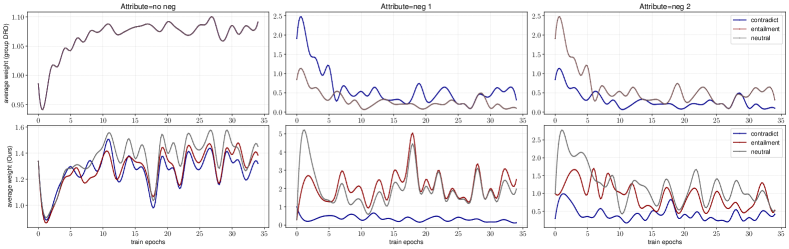
Figure 2: Under the imperfect partition of the MNLI dataset, the aggregated average training weights of instance losses in each group divided by attributes and labels (top: group DRO; bottom: GC-DRO).

Natural Language Inference (NLI). NLI is the task of determining whether a hypothesis is true (entailment), false (contradiction) or undetermined (neutral) given a premise. We use the MultiNLI dataset (Williams et al., 2018) and follow the train/dev/test split in Sagawa et al. (2020a), which results in 206,175 training examples. Gururangan et al. (2018) have shown that there is spurious correlation between the label of contradiction and the presence of negation words (nobody, nothing, no, never) due to annotation artifacts. We further split the negation words into two groups: set 1 (nobody, nothing) and set 2 (no, never) to have more variety in the attributes, i.e. $\mathcal{A}=\{$no negation, negation 1, negation 2$\}$, which together with labels forms 9 groups in the clean partition. We create 3 groups in the imperfect partition as shown in Tab. 2(b), where $G_{1}$ only contains examples from $a=$no negation, while $G_{2}$ and $G_{3}$ contain data from both $a=$negation 1 and $a=$negation 2. This causes a dilemma when upweighting either of the groups.

Toxicity Detection. This task aims to identity various forms of toxic languages (e.g. abusive speech, hate speech), an application with practical and important real-world consequences. Sap et al. (2019) have shown that there is a strong correlation between certain surface markers of English spoken by minority groups and the labels of toxicity. And such biases can be acquired and propagated by models trained on these corpora. We perform experiments on the FDCL18 (Fortuna & Nunes, 2018) dataset, a corpus of 100k tweets annotated with four labels: $\mathcal{Y}=\{$hateful, spam, abusive and normal$\}$. Since the dataset does not contain the dialect information, we follow Sap et al. (2019) and use annotations predicted by the dialect classifier in Blodgett et al. (2016) to label each example as one of four English varieties: $\mathcal{A}=\{$White-aligned, African American (AAE), Hispanic, and Other$\}$. As noted in Sap et al. (2019), these automatically obtained labels correlate highly with self-reported race and provide an accurate proxy for the dialect labels. These dialect attributes and toxicity labels together divide the dataset into 16 groups in the clean partition. To construct the imperfect partitions, we investigate a natural setting where data is divided by the dialect attributes, therefore we have 4 groups in the imperfect partition. The test set of FDCL18 contains some groups that are severely under-represented. In order to make the robust accuracy reliable yet still representative of the under-represented groups, we follow Michel et al. (2021) and combine groups that contain less than 100 samples into a single group to compute robust test accuracies.

6.2 Experimental Setup

We fine-tune pretrained models for object recognition and NLP tasks that achieve high average test accuracies, specifically ResNet18 (He et al., 2016) on CelebA and RoBERTa (Liu et al., 2019) on the MultiNLI and FDCL18 datasets. We select hyperparameters by the robust validation accuracy. For the clean partitions, we set $\alpha=0.2,\beta=0.5$ for all the three tasks. For the imperfect partitions, we set a relatively lower value of $\beta$ to highlight badly performed instances within groups. Specifically, for NLP tasks we set $\alpha=0.5$, $\beta=0.2$ and $0.25$ for NLI and toxicity detection respectively, and for the image task, we set $\alpha=0.2,\beta=0.1$. For more training details, see Appendix E. We measure both the average accuracy over all the test data as well as the robust accuracy (worst accuracy across all groups). Even though different partitions (clean/imperfect) are used at training time, we always evaluate the model’s robust accuracy across groups of the clean partitions of the test data.

We compare with ERM, which minimizes the average training loss on the empirical training distribution, formally

$$\small\mathcal{L}_{\mathrm{ERM}}(\theta)=\mathbb{E}_{(x,y)\sim P_{train}}[\ell(x,y;\theta)]\vspace{-1mm}$$ (7)

We also compare with two variants of group DRO with different objective and optimization procedures: a greedy (Oren et al., 2019) algorithm for CVaR-group DRO and a exponentiated-gradient (EG) (Sagawa et al., 2020a) procedure with full simplex . Note that while previous work (Sagawa et al., 2020a) has found the greedy algorithm is unstable and underperforms EG, we did not observe this issue with our implementation where we took a slight different approach to compute the worst expected loss and we detail this difference in Appendix E.2. In addition, we compare with the resampling method, which optimizes on minibatches sampled from uniform group frequencies, which is often used for imbalanced datasets.

6.3 Main Results

We present the robust and average test accuracies of all three tasks under different partitions in Tab. 3. Models are selected based on the worst-performing accuracy of group (of the clean partition) in the validation set. All the results are averaged over 5 runs with different random seeds. Except for ERM, all the models leverage the group information at training time. First, as expected, ERM models attain high average test accuracies across all the datasets but perform poorly on the worst-case group. Second, we observe that under the clean partition, group DRO models always significantly outperform ERM on the worst-group test accuracy with modest drop in the average test accuracy. And we also note that group DRO optimized with the greedy algorithm performs on par with that optimized by the EG based algorithm. By contrast, the resampling method can not consistently perform well on the worst test groups on all datasets. Furthermore, our method performs similarly to or slightly better than group DRO on all three datasets under the clean partition. Third, under the imperfect partition, neither group DRO nor resampling can perform well in the worst test groups and achieves similar performance to that of ERM models. On the other hand, our method performs significantly better in terms of the robust accuracy on all three datasets, with 5-37 points in improvement over group DRO models. Although the results are worse compared to those under the clean partition, we demonstrate that our method is much more agnostic to the underlying data partitions.

6.4 Analysis

Why does GC-DRO perform well on robust accuracy? In this section, we investigate why group-conditional DRO works well under imperfect partitions. To do this, we first compute the actual weight ($\frac{n_{i}q^{(t)}(g_{i})q^{(t)}(x,y|g_{i})}{\hat{p}^{train(t)}(g_{i})}$ in Alg. 1) applied to each instance $(x_{i},y_{i})$ at every step $t$ for group DRO and our method respectively. The groups in imperfect partitions contain instances from different values of $(a,y)$ and to study the effects of learning weights on the test groups, we aggregate the weights of instances on each group $(a,y)$ (i.e. the clean partition) by taking average over all steps in each epoch. In Fig. 2, we plot the dynamic aggregated weights over the training course learned with the imperfect partition (3 groups, see Tab. 2(b)) of the MNLI dataset. We observe that GC-DRO can assign higher weights to instances that belong to groups of $(a=$negation, $y\neq$ contradiction$)$, which helps prevent the model from learning the spurious correlations between $a=$ negation and $y=$contradiction. On the contrary, group DRO can not accomplish this goal because it can not handle these subgroups inside groups in a fine-grained way.

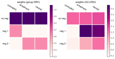
Figure 3: The heatmap of summarized learning weights for different groups from group DRO and our method.

To make this trend more clear, we summarize the weights across all the epochs for each group of $(a,y)$ and present the heat map in Fig. 3. We can see that group DRO focuses on learning from the large group that does not contain negation words but pays less attention to those minority groups. On the contrary, our method encourages the model to learn from minority groups that can help combat spurious features.

	Robust Acc	Average Acc
ERM	34.30 $\pm$ 1.83	79.7 $\pm$ 1.05
resampling	34.20 $\pm$ 2.36	79.4 $\pm$ 1.24
group DRO (EG)	32.84 $\pm$ 2.72	80.5 $\pm$ 0.59
group DRO (greedy)	34.48 $\pm$ 4.69	79.62 $\pm$ 0.59
GC-DRO (ours)	45.06 $\pm$ 6.77	70.7 $\pm$ 4.81

Table 4: Average and robust test accuracies of FDCL18 under the partitions via unsupervised clustering.

On groups produced by unsupervised clustering. We study a more realistic setting where no group information is available and we use an unsupervised clustering algorithm to produce the partitions. Specifically, we first embed the training sentences of the FDCL18 dataset with Sentence-BERT (Reimers et al., 2019), a well-performing semantic sentence embedder, then we use K-means to obtain 8 clusters. In Tab. 4, we show the robust and average accuracy on the test set of the toxicity detection task. Our method once again significantly outperforms other baseline methods on the robust test accuracy, which demonstrates the robustness of GC-DRO under different partitions.

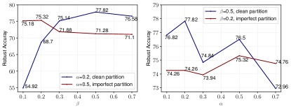
Figure 4: Ablation studies on $\alpha$ and $\beta$ on the MNLI datasets.

Ablation studies on $\alpha$ and $\beta$. We perform ablation studies on the two important hyperparameters $\alpha$ and $\beta$ used in our method. In Fig 4, we fix one value and vary the other and plot the robust test accuracies over 5 random runs (the variance of average test accuracies is very small) on the NLI task. We observe that GC-DRO is less sensitive to different combinations of $\alpha$ and $\beta$ under the imperfect partitions. However, for the clean partitions, a larger $\beta$ and a smaller $\alpha$ tends to yield better performance, as GC-DRO behaves more close to the plain group DRO.

7 Conclusion

Through a mathematical characterization of features used in prediction, we have demonstrated that under covariate shift ERM models can pick up spurious features or miss robust features. The GC-DRO algorithm resulting from this analysis allows for a more flexible uncertainty set that performs consistently well in the worst test group under different partitions. This new understanding of features opens up new avenues in both redesigning our distributionally robust algorithms, and further characterizing possible spurious factors that may influence model robustness, for example through unsupervised learning.

Appendix A Proofs of Theorem 1

Lemma 1.

If $T$ is sufficient statistics, we have $p(Y,X|T)=p(Y|T)\cdot p(X|T)$.

Lemma 2.

If $T$ is sufficient statistics, we have $p(Y|T(X))=p(Y|X)$.

Proof.

Find $T^{\prime}(X)$, s.t. $S(x)=\langle T(X),T^{\prime}(X)\rangle$ is an invertible mapping of $X$, thus $p(Y|X)=p(Y|S(X))=p(Y|T(X),T^{\prime}(X))$. We have,

$$p(Y,T(X),T^{\prime}(X)|T(X))=p(Y|T^{\prime}(X),T(X))p(T^{\prime}(X)|T(X))$$ (8)

From Lemma 1, we have

$$p(Y,T(X),T^{\prime}(X)|T(X))=p(Y|T(X))p(T^{\prime}(X)|T(X))$$ (9)

By (8) and (9), we obtain $p(Y|T^{\prime}(X),T(X))=p(Y|T(X))=p(Y|X)$. ∎

See 1

Proof.

Since there is covariate shift between $p_{\text{ideal}}$ and $p_{\text{train}}$, we have $p_{\text{train}}(Y|X)=p_{\text{ideal}}(Y|X),\forall x\in\mathcal{X}_{train}$. Since $T_{train}(X)$ is MSS of $p_{\text{train}}$ and by Lemma 2, we have $p_{\text{train}}(Y|T_{train}(X))=p_{\text{train}}(Y|X)=p_{\text{ideal}}(Y|X)=p_{\text{ideal}}(Y|T_{ideal}(X)),\forall x\in\mathcal{X}_{train}$. Then $\forall x\in\mathcal{X}_{train},y\in\mathcal{Y}$,

$$p_{\text{train}}(y|T_{ideal}(x)) =\sum\limits_{x^{\prime}:T_{ideal}(x^{\prime})=T_{ideal}(x)}p_{\text{train}}(y|x^{\prime})p_{\text{train}}(x^{\prime}|T(x))$$

$$=\sum\limits_{x^{\prime}:T_{ideal}(x^{\prime})=T_{ideal}(x)}p_{\text{ideal}}(y|x^{\prime})p_{\text{train}}(x^{\prime}|T(x))$$

$$=\sum\limits_{x^{\prime}:T_{ideal}(x^{\prime})=T_{ideal}(x)}p_{\text{ideal}}(y|T(x))p_{\text{train}}(x^{\prime}|T(x))$$

$$=p_{\text{ideal}}(y|T_{ideal}(x))$$ (10)

Then we have

$$H_{train}(Y|T_{train}(X)) =\sum_{x,y}p_{\text{train}}(x,y)[-\log p_{\text{train}}(y|T_{train}(x))]$$

$$=\sum_{x,y}p_{\text{train}}(x,y)[-\log p_{\text{ideal}}(y|T_{ideal}(x))]$$

$$=\sum_{x,y}p_{\text{train}}(x,y)[-\log p_{\text{train}}(y|T_{ideal}(x))]$$

$$=H_{train}(Y|T_{ideal}(X))$$ (11)

From equation A and the definition of sufficient statistics, we have

$$I_{train}(Y;T_{train}(X))=I_{train}(Y;X)=I_{train}(Y;T_{ideal}(X))$$ (12)

Thus, $T_{ideal}(X)$ is the sufficient statistics of $X$ about $Y$ under $p_{\text{train}}$. By definition, we have

$$H_{train}(T_{train}(X)|T_{ideal}(X))=0.$$ (13)

∎

See 1

Proof.

Since $\mathcal{X}_{train}=\mathcal{X}_{ideal}=\mathcal{X}$, with the similar derivation of equation A, we have $\forall x\in\mathcal{X},y\in\mathcal{Y}$

$$p_{\text{ideal}}(y|T_{ideal}(x))=p_{\text{ideal}}(y|T_{train}(x))$$ (14)

Together with Theorem 1, we have $T_{train}(x)$ is also the MSS under $p_{\text{ideal}}$. ∎

Appendix B Connections between MLE and Learning Minimal Sufficient Statistics

B.1 Information Bottleneck (IB) Method

The information bottleneck (IB) method (Tishby et al., 2000) is an information theoretic principle introduced to extract relevant information that an input $X\in\mathcal{X}$ contains about an output random variable $Y\in\mathcal{Y}$. Defined on a joint distribution of $X$ and $Y$, IB learns a mapping function $T(X)$ by optimizing the trade-off between the mutual information $I(X;T)$ and $I(Y;T)$ such that $T(X)$ is a compressed representation of $X$ (quantified by $I(X;T)$) that is most informative about $Y$ (quantified by $I(Y;T)$). Let $T$ be parameterized by $\theta$, the objective of IB optimizes the trade-off between $I(Y;T_{\theta}(X))$ and $I(X;T_{\theta}(X))$:

$$\min_{\theta}-I(Y,T_{\theta}(X))+\beta I(X;T_{\theta}(X))$$ (15)

where $\beta$ is a positive Lagrange multiplier.

Schwartz-Ziv & Tishby (2017) casts finding of minimal sufficient statistics (MSS) $T(X)$ as a constrained optimization problem using data-processing inequality (Cover, 1999):

$$\min_{T(X)}~{}~{}I(T(X);X)$$

$$s.t~{}~{}I(T(X);Y)=I(X;Y)$$ (16)

This corresponds to the IB method (Eq. 15) which extends the notion of relevance between functions of samples and parameters in conventional MSS to any joint distribution of $X$ and $Y$. The IB method provides a computational framework for finding approximate MSS in a soft manner by trading off the sufficiency for $Y$ (I(Y; T(X))) and the minimality of the statistic ($I(X,T(X))$) with the Lagrange multiplier $\beta$ (Schwartz-Ziv & Tishby, 2017; Shamir et al., 2010).

B.2 Connections between MLE and IB

Given that the IB objective is approximately learning MSS in a soft manner, we next build the connections between the popularly adopted maximum likelihood estimation (MLE) in supervised learning and the IB objective. We show that under certain assumptions, MLE is approximating the IB objective defined on the joint distribution of $p_{\text{train}}(X,Y)$.

To facilitate the discussions, we decompose the model parameters into $\theta$ and $\phi$ that denote the parameters of the feature extractor $T_{\theta}(x)$ and the classifier respectively. MLE minimizes the expected negative log probability under $p_{\text{train}}(X,Y)$:

$$\min_{\theta,\phi}\mathbb{E}_{x,y\sim p_{\text{train}}(X,Y)}[-\log p_{\theta,\phi}(x,y)]$$ (17)

$$\iff \min_{\theta,\phi}\mathbb{E}_{x,y\sim p_{\text{train}}(X,Y)}[-\log p_{\phi}(y|T_{\theta}(x))-\log p_{\theta}(x)]$$ (18)

Usually, we only model the conditional distribution $p_{\phi}(Y|X)$ and assume that $p_{\theta}(X)=p_{\text{train}}(X)$ which is independent from $\theta$. With the assumption that $p_{\theta}(x)\propto p^{\beta}(T_{\theta}(x))),\beta>0$, (18) can be rewritten as:

$$\min_{\theta,\phi}\mathbb{E}_{x,y\sim p_{\text{train}}(X,Y)}[-\log p_{\phi}(y|T_{\theta}(x))]+\beta\mathbb{E}_{x\sim p_{\text{train}}(X)}[-\log p(T_{\theta}(x))]$$ (19)

Assume that the neural network parameterized by $\phi$ is a universal function approximator, then we can replace $\min_{\theta,\phi}$ with $\min_{\theta}$ and (19) can be written as:

$$\min_{\theta}H(Y|T_{\theta}(X))+\beta H(T_{\theta}(X))$$ (20)

$$\mathrm{by\;(1)}\;I(Y;T_{\theta}(X))=H(Y)-H(Y|T_{\theta}(X))$$

$$\mathrm{\;\;\;\;\;(2)}\;H(T_{\theta}(X))=I(X;T_{\theta}(X))+H(T_{\theta}(X)|X)=I(X;T_{\theta}(X))$$

$$\iff \min_{\theta}-I(Y;T_{\theta}(X))+\beta I(X;T_{\theta}(X))$$ (21)

We can see that under the assumption of $p_{\theta}(x)\propto p^{\beta}(T_{\theta}(x)))$, the MLE objective can be converted into the same form as the IB objective. In practice, we usually do not model $p_{\text{train}}(X)$ and only optimize the first term $I(Y;T_{\theta}(X))$ in (21). However, previous work (Schwartz-Ziv & Tishby, 2017; Geiger, 2020) has shown that deep neural networks (DNNs) are implicitly minimizing $I(X;T_{\theta}(X))$ with a wide range of activation functions and architectures, which are manifested as a second compression phase during learning with SGD. Thus, we can presumably consider MLE as approximating the IB objective, which is equivalent to learning the MSS on the train distribution $p_{\text{train}}(X,Y)$.

Appendix C Details of the Online Greedy Algorithm for Group DRO

Input : $\alpha$; $m$: total number of groups

Initialize historical average group losses $\hat{L}^{(0)}$; historical estimate of group probabilities $\hat{p}^{train(0)}$; learning rate $\eta$

for $t=1,\cdots,T$ do

       Sample a mini-batch batch $B=({\mathbf{x}},{\mathbf{y}},{\mathbf{g}})$ uniformly from $p_{\text{train}}$

       $\triangleright$ Update the historical vectors of $\hat{L}^{(t)}$ and $\hat{p}^{train(t)}$ for each group $g\in\{1,\cdots,m\}$

       $\hat{L}^{(t)}(g)\leftarrow\mathrm{EMA}(\{\ell({\mathbf{x}}_{i},{\mathbf{y}}_{i};\theta^{(t-1)}):{\mathbf{g}}_{i}=g\},~{}\hat{L}^{(t-1)}(g))$

       $\hat{p}^{train(t)}\leftarrow\mathrm{EMA}(\mathrm{\#samples~{}of~{}each~{}group~{}in~{}B},~{}\hat{p}^{train(t-1)})$

       $\triangleright$ Update the worst-case distribution $q^{(t)}$

       Sort $\hat{p}^{train(t)}$ in the order of decreasing $\hat{L}^{(t)}$ and denote the sorted group indexes $\bm{\pi}$

       $q^{(t)}(g_{\bm{\pi}_{i}})=\min\{\frac{\hat{p}^{train(t)}(g_{\bm{\pi}_{i}})}{\alpha},1-\sum_{j=1}^{i-1}\frac{\hat{p}^{train(t)}(g_{\bm{\pi}_{j}})}{\alpha}\}$

       $\triangleright$ Update model parameters $\theta$

       $\theta^{(t)}=\theta^{(t-1)}-\frac{\eta}{|B|}\sum_{i=1}^{|B|}\frac{q^{(t)}({\mathbf{g}}_{i})}{\hat{p}^{train(t)}({\mathbf{g}}_{i})}\nabla\ell({\mathbf{x}}_{i},{\mathbf{y}}_{i};\theta^{(t-1)})$

end for

Algorithm 2 Online greedy algorithm for group DRO (Oren et al., 2019)

EMA refers to exponential weighted moving average such that $\mathrm{EMA}(v_{1},v_{2})=\gamma v_{1}+(1-\gamma)v_{2}$, where $\gamma\in(0,1)$.

Appendix D Synthetic Experiments: on Investigation Spurious Features under Covariate Shift

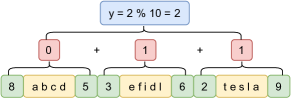
Figure 5: An illustrative example of the synthetic task.

Synthetic Experiments

We design synthetic experiments where data is generated based on the ground-truth rules and different biases are injected. We show that even in the presence of necessary information to learn the rules, the ERM model (specifically, we examine MLE) can still learn spurious features or miss robust features under covariate shift. The synthetic task aims to predict an integer $y\in\{0,\cdots,9\}$ conditioned on a sequence $x$ as shown in Fig. 5. Concretely, $x$ is composed of $m$ chunks, where each chunk $c_{i}$ has $|c_{i}|$ characters that are randomly sampled from an alphabet $\mathcal{V}$. We prepend an integer $c_{i}^{1}$ and append an integer $c_{i}^{2}$ to each chunk $c_{i}$, and both $c_{i}^{1}$ and $c_{i}^{2}$ are uniformly sampled from $[1,10]$. The target integer $y$ is predicted following the rules: each triple of $(c_{i}^{1},c_{i},c_{i}^{2})$ produces an indicator value $d_{i}$; $d_{i}=c_{i}^{2}-c_{i}^{1}$ if $c_{i}^{2}>c_{i}^{1}$, otherwise $d_{i}=0$; then $y=(\sum_{i=1}^{m}d_{i})\mod 10$. We set $3\leq m\leq 6$, $3\leq|c_{i}|\leq 5$ and $|\mathcal{V}|=26$,. We use a one-layer bidirectional LSTM (Hochreiter & Schmidhuber, 1997) to model the input sequence and use the final hidden states of the LSTM to predict the target value. We create training data following the the above description and design two settings that introduce covariate shift to examine if the model can learn the rules with ERM.

(a) Setting 1 — ERM-trained models can miss robust features under covariate shift: We create the training data by imposing $c_{m}^{2}>c_{m}^{1}$ on the last chunk $c_{m}$ of all the training samples. When we create the training data, the rules applied to each chunk are the same as described above, which means that the model does not need to learn additional rules for the last chunk. We are interested in examining whether the model trained with ERM will apply the rules learned from other chunks to the last one or it will miss the robust features of the last chunk. At test time, we evaluate on two groups of test sets: $\mathcal{D}_{out}$ where $c_{m}^{2}\leq c_{m}^{1}$, different from the training data, and $\mathcal{D}_{in}$ where $c_{m}^{2}>c_{m}^{1}$, consistent with the training data. From Tab. 5, we see that the test accuracy on $\mathcal{D}_{out}$ is much lower that that on $\mathcal{D}_{in}$. This demonstrates that the model only learns robust features from chunks $c_{1}^{m-1}$ but misses the robust features of the last chunk $c_{m}$. We conjecture that the model trained with ERM learns in a lazy way where it tries to minimize the entropy of learned features by memorizing patterns and taking shortcuts as discussed further in Appendix B.2.

(b) Setting 2 — ERM-trained models can learn spurious features under covariate shift: In the second setting, we inject spurious patterns into the training data that co-occur with the rules we aim to learn. As both robust rules and spurious patterns co-exist in the training data, we would like to see whether the model picks up the spurious ones or the robust ones. Specifically, each training input sequence has a chunk $c_{j}$ that includes a special segment of characters, e.g. a b. The remainder of $d_{j}=c_{j}^{2}-c_{j}^{1}$ and the sum of all indicators $\sum_{i=1}^{m}d_{i}$ mod by 10 are the same such that the target label $y$ is always the same as the indicator $d_{j}$. Similarly, we test on two cases: i) $\mathcal{D}_{in}$ where every sequence includes a special chunk as in the training set; ii) $\mathcal{D}_{out}$ where characters in each chunk are uniformly sampled. We can see from Tab. 5 that the model learns to use the spurious patterns to predict the target label instead of the general rules.

	$\mathcal{D}_{in}$	$\mathcal{D}_{out}$
Setting 1	99.93 $\pm$ 0.02	14.68 $\pm$ 2.60
Setting 2	100.00 $\pm$ 0.00	10.26 $\pm$ 0.25

Table 5: Test accuracy of the synthetic task.

Appendix E Experimental Details

E.1 Models and Training Details

Model Specific Settings

In our method, we adopt two criterions in GC-DRO to determine when to update $q(x,y|g)$ for each groups: (1) update when the robust validation accuracy drops (2) update at every epoch. With (2), $q(x,y|g)$ is updated more frequently. For MNLI and Celeb-A, we use the second criterion. For FDCL18, we use the first criterion, because this is a relatively smaller dataset and updating $q(x,y|g)$ less frequently makes training more stable. Every time $q(x,y|g)$ is updates, we clear the historical losses in EMA that is used for updating $q(g)$. We use exponentially weighted moving average (EMA) to compute the historical losses for both $q(g)$ and $q(x,y|g)$, for which we denote $\mathrm{EMA}_{\text{G}}$ and and $\mathrm{EMA}_{\text{CG}}$ respectively. As shown above, we use $\gamma$ to denote the coefficient for current value in EMA, thus $1-\gamma$ is used to the historical value. We found that the value of $\gamma$ is an important hyperparameter in some cases to achieve better performance, since the final $q$ distribution is computed through sorting the losses accumulated via EMA. Basically, a higher $\gamma$ pays more attention to the current value. We search over $\{0.1,0.5\}$ for both $\gamma$ used in $\mathrm{EMA}_{\text{G}}$ and $\mathrm{EMA}_{\text{CG}}$ respectively. Through the robust accuracy on the validation set, we set both $\gamma$’s to be 0.5 for the NLP tasks except that for the imperfect partition of toxicity detection we set $\gamma$ used in $\mathrm{EMA}_{\text{G}}$ to be 0.1. For the image task, we set both $\gamma$’s to be 0.1. For the $\gamma$ used in accumulating the historical fractions of groups, we always use a small value 0.01.

Training Details

For the NLP tasks, we finetune a base Roberta model (Liu et al., 2019; Ott et al., 2019) and we segment the input text into the sub-word tokens using the tokenization described in (Liu et al., 2019). During training, we sample minibatches that contain at most 4400 tokens. We train MNLI using Adam (Kingma & Ba, 2014) with an intitial learnig rate of $1e-5$ for 35 epochs and FDCL18 for 45 epochs, and we linearly decay the learning rate at every step until the end of training. For the image task, we fine-tune a ResNet-18 (He et al., 2016) for 50 epochs with batch size of 256. We use SGD with learning rate of $1e-4$. At the end of every epoch, we evaluate the robust accuracy on the validation set. We train on one Volta-16G GPU and it takes around 2 - 5 hours to finish one experiments for different datasets.

E.2 Implementation of the Group DRO Loss

We referred to the implementation of greedy group DRO in Sagawa et al. (2020a), where they use the exact formulation in Eq. 5 to compute the expected loss, which leads to inferior performance compared to the exponentiated-gradient based optimization as reported in Sagawa et al. (2020a). The implementation computed the final loss by first computing the average loss over instances for each group (MC for the inner expectation), then compute the full expected value over the averaged group loss, as shown below:

$$\vspace{-3mm}\ell({\mathbf{x}},{\mathbf{y}},{\mathbf{g}};\theta)=\sum_{g}q(g)\bar{\ell}(g)=\sum_{g}q(g)\frac{1}{C_{g}}\sum_{\{i,\forall{\mathbf{g}}_{i}=g\}}{\ell({\mathbf{x}}_{i},{\mathbf{y}}_{i};\theta)},$$ (22)

where $({\mathbf{x}},{\mathbf{y}},{\mathbf{g}})$ is a mini-batch and $C_{g}$ is the number of samples that belong to group $g$ in the mini-batch. We can see that instances that belong to different groups are weighted correspondingly by the number of group size in a mini-batch. This causes that instances in large group get unfairly lower weights, especially when its probability in the $q$ distribution is low. We fix this by directly computing the expected loss over the joint distribution of $q(x,y,g)$, i.e. $\mathbb{E}_{(x_{i},y_{i},g_{i})\sim q(x,y,g)}\ell(x_{i},y_{i},g_{i};\theta)=\mathbb{E}_{(x_{i},y_{i},g_{i})\sim p_{\text{train}}(x,y,g)}\frac{q(x_{i},y_{i},g_{i})}{p_{\text{train}}(x_{i},y_{i},g_{i})}\ell(x_{i},y_{i},g_{i})$. Specifically, we do this by summing over all the importance weighted instance losses using corresponding group weights and taking average. This allows us to obtain unbiased gradient estimates of $\theta$.

$$\frac{1}{N}\sum_{i}\frac{q({\mathbf{g}}_{i})}{p_{\text{train}}(g_{i})}\ell({\mathbf{x}}_{i},{\mathbf{y}}_{i};\theta)$$ (23)

References

- Achille & Soatto (2018) Achille, A. and Soatto, S. Emergence of invariance and disentanglement in deep representations. The Journal of Machine Learning Research, 19(1):1947–1980, 2018.
- Adragni & Cook (2009) Adragni, K. P. and Cook, R. D. Sufficient dimension reduction and prediction in regression. Philosophical Transactions of the Royal Society A: Mathematical, Physical and Engineering Sciences, 367(1906):4385–4405, 2009.
- Arjovsky et al. (2019) Arjovsky, M., Bottou, L., Gulrajani, I., and Lopez-Paz, D. Invariant risk minimization. arXiv preprint arXiv:1907.02893, 2019.
- Bahng et al. (2020) Bahng, H., Chun, S., Yun, S., Choo, J., and Oh, S. J. Learning de-biased representations with biased representations. In International Conference on Machine Learning, pp. 528–539. PMLR, 2020.
- Beery et al. (2018) Beery, S., Van Horn, G., and Perona, P. Recognition in terra incognita. In Proceedings of the European Conference on Computer Vision (ECCV), pp. 456–473, 2018.
- Bellot & van der Schaar (2020) Bellot, A. and van der Schaar, M. Generalization and invariances in the presence of unobserved confounding. arXiv preprint arXiv:2007.10653, 2020.
- Ben-Tal et al. (2013) Ben-Tal, A., Den Hertog, D., De Waegenaere, A., Melenberg, B., and Rennen, G. Robust solutions of optimization problems affected by uncertain probabilities. Management Science, 59(2):341–357, 2013.
- Blodgett et al. (2016) Blodgett, S. L., Green, L., and O’Connor, B. Demographic dialectal variation in social media: A case study of african-american english. In Proceedings of the 2016 Conference on Empirical Methods in Natural Language Processing, pp. 1119–1130, 2016.
- Buolamwini & Gebru (2018) Buolamwini, J. and Gebru, T. Gender shades: Intersectional accuracy disparities in commercial gender classification. In Conference on fairness, accountability and transparency, pp. 77–91, 2018.
- Cover (1999) Cover, T. M. Elements of information theory. John Wiley & Sons, 1999.
- Cvitkovic & Koliander (2019) Cvitkovic, M. and Koliander, G. Minimal achievable sufficient statistic learning. volume 97, pp. 1465–1474. PMLR, 2019.
- David et al. (2010) David, S. B., Lu, T., Luu, T., and Pál, D. Impossibility theorems for domain adaptation. In Proceedings of the Thirteenth International Conference on Artificial Intelligence and Statistics, pp. 129–136. JMLR Workshop and Conference Proceedings, 2010.
- Duchi et al. (2016) Duchi, J., Glynn, P., and Namkoong, H. Statistics of robust optimization: A generalized empirical likelihood approach. arXiv preprint arXiv:1610.03425, 2016.
- Duchi et al. (2019) Duchi, J. C., Hashimoto, T., and Namkoong, H. Distributionally robust losses against mixture covariate shifts. 2019.
- Dynkin (2000) Dynkin, E. B. Necessary and sufficient statistics for a family of probability distributions. Selected Papers of EB Dynkin with Commentary, 14:393, 2000.
- Fortuna & Nunes (2018) Fortuna, P. and Nunes, S. A survey on automatic detection of hate speech in text. ACM Computing Surveys (CSUR), 51(4):1–30, 2018.
- Gao & Kleywegt (2016) Gao, R. and Kleywegt, A. J. Distributionally robust stochastic optimization with wasserstein distance. arXiv preprint arXiv:1604.02199, 2016.
- Geiger (2020) Geiger, B. C. On information plane analyses of neural network classifiers–a review. arXiv preprint arXiv:2003.09671, 2020.
- Goyal et al. (2017) Goyal, Y., Khot, T., Summers-Stay, D., Batra, D., and Parikh, D. Making the v in vqa matter: Elevating the role of image understanding in visual question answering. In Proceedings of the IEEE Conference on Computer Vision and Pattern Recognition, pp. 6904–6913, 2017.
- Gururangan et al. (2018) Gururangan, S., Swayamdipta, S., Levy, O., Schwartz, R., Bowman, S., and Smith, N. A. Annotation artifacts in natural language inference data. In Proceedings of the 2018 Conference of the North American Chapter of the Association for Computational Linguistics: Human Language Technologies, Volume 2 (Short Papers), pp. 107–112, 2018.
- Hashimoto et al. (2018) Hashimoto, T., Srivastava, M., Namkoong, H., and Liang, P. Fairness without demographics in repeated loss minimization. In International Conference on Machine Learning, pp. 1929–1938, 2018.
- He et al. (2016) He, K., Zhang, X., Ren, S., and Sun, J. Deep residual learning for image recognition. In Proceedings of the IEEE conference on computer vision and pattern recognition, pp. 770–778, 2016.
- Hochreiter & Schmidhuber (1997) Hochreiter, S. and Schmidhuber, J. Long short-term memory. Neural computation, 9(8):1735–1780, 1997.
- Hu et al. (2018) Hu, W., Niu, G., Sato, I., and Sugiyama, M. Does distributionally robust supervised learning give robust classifiers? In International Conference on Machine Learning, pp. 2029–2037. PMLR, 2018.
- Hu & Hong (2013) Hu, Z. and Hong, L. J. Kullback-leibler divergence constrained distributionally robust optimization. Available at Optimization Online, 2013.
- Husain (2020) Husain, H. Distributional robustness with ipms and links to regularization and gans. In Proceedings of the 34th Annual Conference on Neural Information Processing Systems (NIPS), 2020.
- Kingma & Ba (2014) Kingma, D. P. and Ba, J. Adam: A method for stochastic optimization. arXiv preprint arXiv:1412.6980, 2014.
- Koenecke et al. (2020) Koenecke, A., Nam, A., Lake, E., Nudell, J., Quartey, M., Mengesha, Z., Toups, C., Rickford, J. R., Jurafsky, D., and Goel, S. Racial disparities in automated speech recognition. Proceedings of the National Academy of Sciences, 117(14):7684–7689, 2020.
- Koh et al. (2020) Koh, P. W., Sagawa, S., Marklund, H., Xie, S. M., Zhang, M., Balsubramani, A., Hu, W., Yasunaga, M., Phillips, R. L., Beery, S., et al. Wilds: A benchmark of in-the-wild distribution shifts. arXiv preprint arXiv:2012.07421, 2020.
- Kolchinsky et al. (2019) Kolchinsky, A., Tracey, B. D., and Van Kuyk, S. Caveats for information bottleneck in deterministic scenarios. In International Conference on Learning Representations, 2019.
- Kullback & Leibler (1951) Kullback, S. and Leibler, R. A. On information and sufficiency. The annals of mathematical statistics, 22(1):79–86, 1951.
- Lewis (2013) Lewis, D. Counterfactuals. John Wiley & Sons, 2013.
- Liu et al. (2019) Liu, Y., Ott, M., Goyal, N., Du, J., Joshi, M., Chen, D., Levy, O., Lewis, M., Zettlemoyer, L., and Stoyanov, V. Roberta: A robustly optimized bert pretraining approach. arXiv preprint arXiv:1907.11692, 2019.
- Liu et al. (2015) Liu, Z., Luo, P., Wang, X., and Tang, X. Deep learning face attributes in the wild. In Proceedings of the IEEE international conference on computer vision, pp. 3730–3738, 2015.
- Lopez-Paz (2016) Lopez-Paz, D. From dependence to causation. PhD thesis, University of Cambridge, 2016.
- Lovering et al. (2021) Lovering, C., Jha, R., Linzen, T., and Pavlick, E. Predicting inductive biases of pre-trained models. In International Conference on Learning Representations (ICLR), 2021.
- McCoy et al. (2019) McCoy, T., Pavlick, E., and Linzen, T. Right for the wrong reasons: Diagnosing syntactic heuristics in natural language inference. In Proceedings of the 57th Annual Meeting of the Association for Computational Linguistics, pp. 3428–3448, 2019.
- Michel et al. (2021) Michel, P., Hashimoto, T., and Neubig, G. Modeling the second player in distributionally robust optimization. In International Conference on Learning Representations (ICLR), 2021.
- Oren et al. (2019) Oren, Y., Sagawa, S., Hashimoto, T. B., and Liang, P. Distributionally robust language modeling. In Conference on Empirical Methods in Natural Language Processing (EMNLP), Hong Kong, November 2019.
- Ott et al. (2019) Ott, M., Edunov, S., Baevski, A., Fan, A., Gross, S., Ng, N., Grangier, D., and Auli, M. fairseq: A fast, extensible toolkit for sequence modeling. In Proceedings of NAACL-HLT 2019: Demonstrations, 2019.
- Reimers et al. (2019) Reimers, N., Gurevych, I., Reimers, N., Gurevych, I., Thakur, N., Reimers, N., Daxenberger, J., and Gurevych, I. Sentence-bert: Sentence embeddings using siamese bert-networks. In Proceedings of the 2019 Conference on Empirical Methods in Natural Language Processing. Association for Computational Linguistics, 2019.
- Rockafellar et al. (2000) Rockafellar, R. T., Uryasev, S., et al. Optimization of conditional value-at-risk. Journal of risk, 2:21–42, 2000.
- Sagawa et al. (2020a) Sagawa, S., Koh, P. W., Hashimoto, T. B., and Liang, P. Distributionally robust neural networks for group shifts: On the importance of regularization for worst-case generalization. In International Conference on Learning Representations (ICLR), Addis Ababa, Ethiopia, April 2020a.
- Sagawa et al. (2020b) Sagawa, S., Raghunathan, A., Koh, P. W., and Liang, P. An investigation of why overparameterization exacerbates spurious correlations. In International Conference on Machine Learning (ICML), July 2020b.
- Sap et al. (2019) Sap, M., Card, D., Gabriel, S., Choi, Y., and Smith, N. A. The risk of racial bias in hate speech detection. In Proceedings of the 57th annual meeting of the association for computational linguistics, pp. 1668–1678, 2019.