Soft hydraulics: from Newtonian to complex fluid flows through compliant conduits

Abstract

Microfluidic devices manufactured from soft polymeric materials have emerged as a paradigm for cheap, disposable and easy-to-prototype fluidic platforms for integrating chemical and biological assays and analyses. The interplay between the flow forces and the inherently compliant conduits of such microfluidic devices requires careful consideration. While mechanical compliance was initially a side-effect of the manufacturing process and materials used, compliance has now become a paradigm, enabling new approaches to microrheological measurements, new modalities of micromixing, and improved sieving of micro- and nano-particles, to name a few applications. This topical review provides an introduction to the physics of these systems. Specifically, the goal of this review is to summarize the recent progress towards a mechanistic understanding of the interaction between non-Newtonian (complex) fluid flows and their deformable confining boundaries. In this context, key experimental results and relevant applications are also explored, hand-in-hand with the fundamental principles for their physics-based modeling. The key topics covered include shear-dependent viscosity of non-Newtonian fluids, hydrodynamic pressure gradients during flow, the elastic response (deformation and bulging) of soft conduits due to flow within, the effect of cross-sectional conduit geometry on the resulting fluid–structure interaction, and key dimensionless groups describing the coupled physics. Open problems and future directions in this nascent field of soft hydraulics, at the intersection of non-Newtonian fluid mechanics, soft matter physics, and microfluidics, are noted.

Keywords: Microfluidics, non-Newtonian fluids, fluid–structure interactions, low-Reynolds-number hydrodynamics, soft hydraulics

1 Introduction

Microfluidics, which concerns the manipulation of small (e.g., nanoliter) volumes of fluids at small (e.g., micron) scales [1, 2], “exploded” around the turn of the century. The number of papers published annually grew ten-fold from 1994 to 2004 [3, p. 7], with another factor of almost ten reached by 2020, according to the Web of Science. Microfluidics has disrupted [4] fields ranging from cellular and developmental biology [5] to logical circuits [6, 7] to chemical and biological warfare deterrents [8], to name a few. The microfluidic technologies market was valued at $18 billion in 2020 [9]. Much of microfluidics has been enabled by polymeric gels made from polydimethylsiloxane (PDMS) (commercially available as the SYLGARD™ 184 silicone elastomer). PDMS allows cheap and rapid manufacture with fine geometric control (down to the nanoscale) [10, 11] and tunable mechanical properties [12]. Figure 1 shows an example PDMS-based microfluidic chip costing on the order of $10 and designed to detect the human immunodeficiency virus (HIV) and methicillin-resistant Staphylococcus aureus (MRSA).

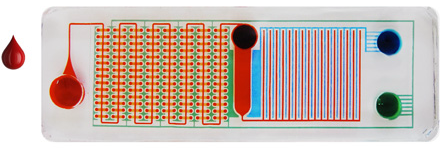
Figure 1: Schematic of a “self-powered integrated microfluidic point-of-care low-cost enabling (SIMPLE) chip” designed for medical diagnostics and able to detect HIV and MRSA at a cost of about $10 per chip [13, 14]. The entire device fits on a standard microscope slide, having dimensions about $25\times 75$ mm. Blood is input in the reservoir on the left, reagents are placed in the middle reservoir, the tubing connected to the voids on the right is a battery vacuum system used to drive the flow. Microchannels are highlighted by colors. Reproduced from [14] with permission from AAAS.

Being made from polymeric materials (e.g., PDMS), channels in microfluidic devices are therefore soft [15] with a Young’s modulus $E\approx 0.3$ to $2$ MPa [16, 17]. That is to say, these materials easily deform under an applied load. In some applications, the device’s compliance can lead to blurring of high-speed optical imaging of its interior [18] or restrict its structural viability [19, 20]. In other applications, however, flexibility is a crucial advantage to be exploited in the design of implantable and wearable electronics [21, 22], or to emulate soft biological tissues in organs-on-a-chip [23, 24]. The salient physics at hand is that the fluid’s pressure forces cause an elastic structure (immersed in a flow or bounding it) to deform, which in turn modifies the flow, as shown schematically in figure 2. This is an example of a fluid–structure interaction [25, 26]. In some fields, another term for this phenomenon is elastohydrodynamics [27].

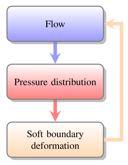
Figure 2: Schematic of the fundamental feedback mechanism of two-way-coupled fluid–structure interaction between an internal fluid flow and the elastic boundaries of the soft flow conduit; styled after a diagram of Fung [28, figure 3.4:2].

In this context, the present topical review specifically aims to address the interaction of non-Newtonian fluid flows and their soft confining boundaries. The discussion below is centered on the fundamental physics and seeks to enable a theoretical understanding of these coupled multi-physics phenomena. The goal is to provide the reader an understanding of key experimental results and relevant applications hand-in-hand with the fundamental principles for modeling, interpretation and design. In doing so, it is expected that the review will enable the reader to identify and pursue open problems in this nascent field of soft hydraulics, at the intersection of non-Newtonian fluid mechanics, soft matter physics, and microfluidics.

1.1 Scope of the review

The key topics covered in this review are:

• the hydraulic–electric circuit analogy (section 3.1);

• the basics of non-Newtonian (complex) fluid rheology, focusing on steady flows (section 3.2);

• the lubrication approximation, flow in long slender conduits, and the relation between the flow rate and the hydrodynamic pressure gradient therein (sections 3.3 and 3.4);

• the elastic response (deformation and bulging) of soft conduits due to flow within (section 3.5), including the effect of the flow conduit’s cross-sectional geometry on the resulting fluid–structure interaction;

• the resulting basic laws of soft hydraulics for flow in compliant conduits (section 3.6);

• a sampling of key applications involving non-Newtonian fluid flows in soft hydraulic conduits (section 4);

• and advanced topics related to the physics of these flows (section 5), leading into current open problems and future directions (section 6).

Naturally, a number of topics cannot be covered in this review. Specifically, manufacturing techniques [29], design of microfluidics chips, and biomicrofluidics (see [30, chapter 8] and [31]) are out of scope here. However, many of these topics are covered in resources beyond the current review that are now briefly summarized.

Important overviews of the pioneering 1990s research on micro-electro-mechanical systems (MEMS) are given by Ho and Tai [32] and Gad-el-Hak [33]. Stone et al. [1, 34] provide a detailed look at the flow physics in rigid hydraulic conduits, with applications of microfluidics to the (then) emerging technology of lab-on-a-chip. Squires and Quake [2] take a deep-dive into (nearly) all flow physics encountered in microfluidics. Abgrall and Gué [35] give a complementary review (to [1, 2]) of the requisite micro-manufacturing techniques. The multiphysics couplings occurring in microfluidic systems, of which the fluid–solid coupling detailed in section 3 is one example, has led to the introduction of the term “nonlinear microfluidics,” overviews of which can be found in [36, 37]. The role of such nonlinear elastohydrodynamic effects on dynamic force measurements (with implications for, e.g., atomic force microscopes and surface forces apparatuses) are reviewed by Wang et al. [38, 39].

Biological and physiological implications of the coupling betwee flow and compliant boundaries (such as arteries and airways) are expounded upon by Grotberg and Jensen [40] and Hazel and Heil [41] (see also [25, chapter 8]), building upon the research program initiated by Shapiro [42] and Pedley [43]. Lauga and Powers [44] discuss related problems arising from the swimming of flagellated microorganisms in complex fluids. Flexible microelectronics benefitting from understanding the physics of microscale fluid–structure interactions are reviewed by Fallahi et al. [45]. The foundational reviews on PDMS as a versatile soft polymeric material for microfluidics and the manufacture of flow conduits from it using soft lithography are given by McDonald and Whitesides [10] and Xia and Whitesides [15], respectively. Recent PDMS-based microfluidics designs and applications are summarized by Raj M and Chakraborty [46], while the decadal review (2007–2017) by Karan et al. [47] focuses on select advances in the five categories of “microchannels, tubes, squeeze flow, cylinder near wall and thin structures (membranes, sheets, etc.).”

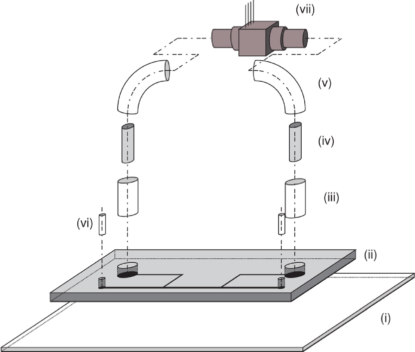
Figure 3: A schematic depicting a microfluidic chip on a glass slide (i) with a single main channel embedded in a PDMS layer (ii). A high-pressure syringe pump was connected to the channel’s inlet port (vi) to maintain the flow rate. External tubing, connectors and components are needed to measure the pressure drop for a given flow rate, accounting for the flow-induced deformation. To this end, a transducer port (iii) is connected via a tubing (iv,v) to a pressure transducer (vii), which makes the pressure drop measurement. Reproduced from Cheung P, Toda-Peters K and Shen A Q 2012 Biomicrofluidics 6 026501 [48], with permission from AIP Publishing © 2012.

Two key recent textbooks, suitable for teaching an upper undergraduate or introductory graduate level course in this field are those by Bruus [49] and Kirby [50], building upon the earlier books by Karniadakis et al. [51], Nguyen and Wereley [3], and Tabeling [52]. It should be noted, however, that these textbooks do not discuss non-Newtonian fluid flows, beyond mentioning the concept.

2 Experimental observations: the need to understand non-Newtonian soft hydraulics

Context for and the motivation to study non-Newtonian fluid flow in soft hydraulic conduits, was discussed by Anand et al. [53]. Specifically, recent experimental papers were reviewed to highlight the lack of broadly applicable predictive physical theory for non-Newtonian fluid flows through soft hydraulic conduits. A schematic of a typical setup of such an experiment is shown in figure 3.

The first example is the experimental study by Raj and Sen [54]. They performed experiments of non-Newtonian fluid flow in a rectangular microchannel with three rigid walls and a compliant top wall, which was manufactured from PDMS (Young’s moduli of $E=1.362$ MPa and $E=1.184$ MPa were quoted for the two wall thicknesses used). A 0.1% polyethylene oxyde (PEO) solution, which exhibits shear thinning (to be introduced in section 3.2) was used as the working fluid. The pressure drop along the microchannel was measured in $12$ mm increments, over its $L=30$ mm length, by a series of differential pressure sensors. As will become important in section 3.3, the microchannel in this experiment was long and thin: having a cross-section of fixed width $w$ between $0.5$ and $2$ mm and undeformed height $h_{0}$ of $83$ $\mu$m. The deformation of the compliant top wall was measured using fluorescence microscopy. Raj and Sen [54] also proposed a mathematical model for the pressure drop across the length of the microchannel, as a function of the flow rate (and the various material and geometric parameters) for Newtonian fluids. However, the model was not generalized to apply to the non-Newtonian experiments.

Kiran Raj et al. [55] carried out experiments on non-Newtonian fluid flow in a compliant cylindrical conduit. They used 0.04% by weight solution of Xanthan gum into deionized water as a blood-analog fluid with shear-thinning properties. A microtube of length $L=27$ mm and diameter $a\approx 500$ $\mu$m was fabricated from PDMS by pull-out soft lithography. Two PDMS mixtures were used, yielding Young’s moduli of $E=2.801$ MPa and $E=0.157$ MPa. A one-way coupled theory to calculate the deformation from the known pressure drop, (as a function of the imposed flow rate) was also proposed. However, the flow regimes investigated in [55] exhibited only weak fluid–structure interaction, and thus deviations from the ideal Hagen–Poiseuille law are small.

Del Giudice et al. [56] also performed experiments with PEO solutions, which exhibit shear thinning, in square cross-section PDMS microchannels ($E\approx 1$ MPa was reported). They demonstrated that the channel’s maximum height increases by $\approx 2$% under a pressure drop $\Delta p\approx 23$ kPa for a 0.5% PEO solution, while the increase is $\approx 12$% under a pressure drop $\Delta p\approx 120$ kPa for a 1.6% PEO solution. They conclude that this effect is significant and should be modeled physically.

Most recently, Nahar et al. [57] performed experiments with 1.4% carboxymethyl cellulose (CMC) and 0.01% polyacrylamide (PAA) aqueous solutions, which exhibit shear thinning, in silicone elastic tubes ($E=4.7$ MPa). They demonstrated the strong effect of fluid rheology by comparing to a flow of a reference Newtonian fluid (a 19% polyethylene glycol (PEG) aqueous solution). Specifically, when a transmural pressure of 105 mbar between the inside and outside of the tube was applied, the tube’s cross-sectional area decreased six times as much for both non-Newtonian fluid flows, compared to the case of the reference Newtonian flow. The observation was rationalized by noting that shear-thinning fluids have a smaller outlet pressure (drop), which is correlated to stronger compressive downstream transmural pressures. A theory for this effect was not provided.

Therefore, despite the early experimental work by Koo and Kleinstreuer [58] noting that “Non-Newtonian fluid effects are expected to be important for polymeric liquids and particle suspension flows,” prior experimental measurements on non-Newtonian effects in soft hydraulic conduits (e.g., [54, 56, 57]) have not been fully rationalized by theory. Additionally, these experiments employ only shear-thinning fluids and no similar experiments with viscoelastic fluids (to be discussed in section 3.2.2) appear to have been conducted in either rigid or compliant conduits. Therefore, a clear knowledge gap remains at the intersection of non-Newtonian fluid mechanics and soft matter physics. This research field is still in its infancy, but progress has been made in the last few years. Specifically, the fluid–structure interaction problem has been analyzed, and predictive theories are now becoming available, reducing the three-dimensional (3D) coupled problem to an ordinary differential equation (ODE) for the hydrodynamic pressure, for different types of compliant conduits (e.g., microchannels or microtubes). Next, the building blocks of these theories are reviewed.

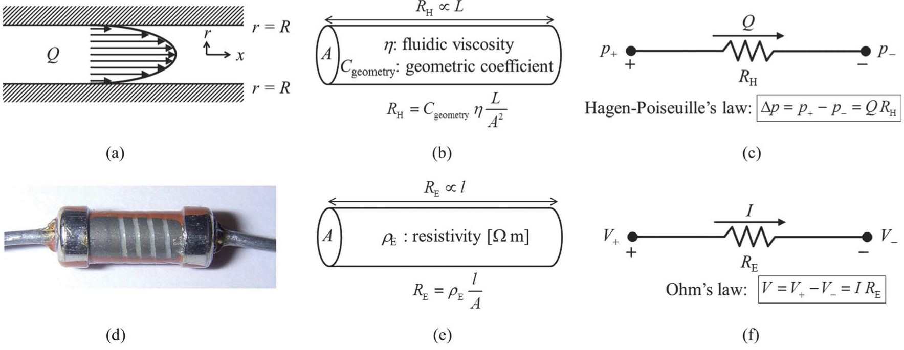
Figure 4: (a) A steady viscous Newtonian fluid flow in a channel or tube and (d) a “partially exposed Tesla TR-212 1 k$\Omega$ carbon film resistor.” (b,e) Analogy between hydraulic resistance and electric resistance, respectively. (c,f) The corresponding circuit notations. The Hagen–Poiseuille law (1) and (3) is the hydraulic equivalent of Ohm’s law (2). In (b), $C_{\mathrm{geometry}}=8\pi$ for a circular flow conduit. Reproduced from [59] with permission from The Royal Society of Chemistry © 2012.

It should be noted that the problem of non-Newtonian elastohydrodynamic lubrication also comes up in tribology [60]. However, these problems involve thin fluid films under extreme pressures and under non-isothermal conditions, in which the fluid behavior can be quite different from the microfluidic setting considered herein. Additionally, tribology problems consider complex deformations, including wall-to-wall contact, and wear (degradation of the fluid and flow conduit), which are not generally expected to occur in microchannels under normal flow conditions. One common problem between tribology and microfluidics could be roll coating flows with deformable substrates [61, 62].

3 Predictive physical theories and models

To review our current understanding of the interaction of non-Newtonian (complex) fluid flows and their soft confining boundaries, in this section, it is helpful to start with the established results on Newtonian fluid flows, and build up from there.

3.1 The hydraulic–electric circuit analogy

A powerful pedagogical analogy for understanding pipe flows is the analogy between the laminar flow of a Newtonian fluid through a pipe and the flow of electrons in a conductor. Figure 4 shows a schematic of this analogy. The basic laws of fluid mechanics dictate that, for a pipe of fixed cross-section, the pressure difference $\Delta p$ needed to maintain a steady volumetric flow rate $q$ through it obeys

$$\Delta p=R_{h}q,$$ (1)

where $R_{h}$ is the hydraulic resistance [49, section 4.2]. The limits of applicability of (1) are explored throughout the review. Indeed, this basic law has the same form as Ohm’s law, which states that the voltage difference $\Delta V$ needed to maintain a steady electrical current $I$ through a conductor with known resistance to the motion of electrons, obeys

$$\Delta V=R_{e}I,$$ (2)

where $R_{e}$ is the electrical resistance of the wire [63, section 4.3].

Thus emerges a parallel between a hydraulic and an electrical circuit: a pump provides $\Delta p$ and a battery provide $\Delta V$; the former drives the flow $q$ of a fluid, while the latter drives the electrical current (“flow” of electrons) $I$. The resistance to conduction by a real material parallels the resistance to internal flow due to the fluid’s viscous forces (friction), in particular at the bounding surfaces. Of course, the physical underpinnings of each phenomenon are entirely different, nevertheless this analogy allows for the reduced-order modeling of fluidic systems, in particular in microfluidics [64, 59]. Kirchhoff’s currents and voltage laws at circuit junctions take on the same form for flow rates and pressures where pipes meet (due to conservation of mass and energy) [49, section 4.7].

Now, for a rigid pipe, the hydraulic resistance is a known function of the pipe’s cross-sectional geometry. Figure 5 shows example cross-sectional geometries of pipes, and $R_{h}$ calculated for each. Specifically, for the case of a rigid cylindrical pipe, (1) holds with

$$R_{h}=\frac{8\eta_{0}L}{\pi a^{4}},$$ (3)

yielding the well-known Hagen–Poiseuille law for Newtonian fluids [65]. Further exact results are possible for a number of “exotic” shapes, shown in figure 5, by solving the basic equations of fluid mechanics exactly in unidirectional (fully-developed) flow [66, 67, 68, 69, 49].

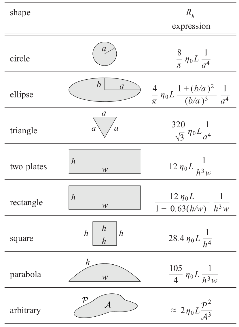
Figure 5: Analytical formulas for the hydraulic resistance $R_{h}$ for steady viscous flow of Newtonian fluids with constant dynamic shear viscosity $\eta_{0}$ through rigid conduits of different cross-section and fixed axial length $L$ (into the page); based on exact solutions for the fully-developed flow profile in a duct [66, section 2-5]. Reprinted and adapted from [49] with permission from Oxford University Press.

But, what if the resistance were to depend on the pressure drop itself (or the flow rate)? Such behavior would correspond to a flow-responsive circuit element, i.e., a “programmable” resistor [70]. Ajdari [71] recognized that two possible ways to generate such a nonlinear response is to employ non-Newtonian fluids and/or to allow the channel walls to deform elastically. In fact, this nonlinear behavior can be achieved in soft microfluidic devices, as demonstrated for both steady [17, 72] and unsteady [73, 74, 75] Newtonian fluid flow. The case of a non-Newtonian working fluid has not been addressed in such detail, in part because the basic hydraulic–electric analogy, which has been so successful in understanding and designing microfluidic circuits with Newtonian fluids [76, 71, 59, 49], requires modifications.

In the remainder of this section, the key physics that enable a predictive theory of microscale flows of non-Newtonian fluids through compliant conduits are summarized, and it is demonstrated how to generalize (1) and (3). Importantly, two modifications emerge: (i) a modification of the “hydraulic Ohm’s law” (1) due to the rheology of the non-Newtonian fluid, and (ii) a modification of the resistance $R_{h}$ due to the deformation of the compliant boundaries of the conduit.

3.2 Rheological behavior of fluids

The standard textbook reference on this topic is by Bird, Armstrong and Hassager [77], with other helpful textbooks by Larson [78] and Chhabra and Richardson [79]. Owens and Phillips [80] cover both the fundamentals of rheology and computational aspects. An exhaustive handbook entry by Nijenhuis et al. [81] describes the experimental interrogation of non-Newtonian fluids. The relevance of non-Newtonian (complex) fluids to microfludics and the basic equations of their flows are briefly discussed in encyclopedia entries by Anna [82] and Chakraborty [83], respectively.

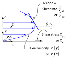
(a)

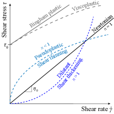
(b)

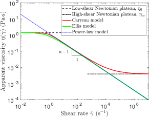
(c)

Figure 6: (a) Sketch of a unidirectional velocity profile $v_{z}$, for both a Cartesian $(x,y,x)$ and a cylindrical axisymmetric $(r,\theta,z)$ coordinate system, and the attendant definition of the shear rate $\dot{\gamma}$. (b) Schematic representation of the variation of the shear stress $\tau$ with the shear rate $\dot{\gamma}$ highlighting that the effective (apparent) viscosity $\eta=\tau/\dot{\gamma}\neq const.$ for time-independent non-Newtonian fluids. (c) Quantitative plot of the three representative models for $\eta(\dot{\gamma})$ considered in the text, see table 1 for notation, styled after a figure by Boger [84]. The rheological model parameter values used are similar to those obtained in [84] for a 0.4% polyacrylamide solution ($\eta_{0}\approx 1.425$ Pa$\cdot$s, $\eta_{\infty}\approx 4\times 10^{-3}$ Pa$\cdot$s, $\tau_{1/2}\approx 1.211$ Pa, $n_{e}\approx 2.43$, $n\approx 0.412$, $K\approx 1.295$ Pa$\cdot$sⁿ, and $\lambda_{r}\approx 1.177$ s). Note the logarithmic axes. The triangle indicating the slope is not to scale.

Newton’s law of viscosity states that the shear stress $\tau$ (resistance to flow and deformation) is proportional to the shear rate of strain $\dot{\gamma}$ (a measure of the deformation of fluid elements under flow) [85]. Although both $\tau$ and $\dot{\gamma}$ are, in fact, tensorial quantities [68, 86, 49], for the purposes of this subsection, they are considered to be the representative (dominant) scalar components of the respective tensors for a given flow. The proportionality constant is the shear viscosity $\eta_{0}$, hence $\tau=\eta_{0}\dot{\gamma}$. The latter relation between shear stress and shear rate of strain is termed the constitutive equation. Many engineering fluids (water, air, glycerol) obey Newton’s law. However, in microfluidics, one deals with complex fluids. Complex fluid are non-Newtonian, which simply means that they do not obey Newton’s law of viscosity.

The technological focus in microfluidics has been on “miniaturizing assays to analyze the biological, physical, and chemical properties of DNA, proteins, and biopolymers in solution, as well as suspensions of cells and bioparticles” [82]. Nominally, when polymers, particles or cells are added to a solution, its viscosity increases. However, the stretching of initially coiled polymers (or deformation and flow-alignment of cells) under shear flow leads to a decrease of the viscosity with shear rate (termed shear thinning). While the shear-dependent viscosity effect may be different in extensional flows, shear flows are the most relevant class in the present context of long and thin microchannels. Further, these effects can be time-dependent (transient) as the polymers and cells relax back to equilibrium. These observations identify the critical need for understanding non-Newtonian fluid flows in microfluidics. Chip-based technologies for genomic analysis (including, but not limited, to DNA sequencing and polymerase chain reactions (PCR) detection methods) go by the name biomicroelectromechanical systems (bioMEMS) [87]. DNA sequencing and PCR detection have also benefited from advances in micropipetting technology, which has been impacted by new understanding of nonstandard inkjet printers that can generate microscopic droplets of complex fluids [88].

Thus, a common complex fluid encountered in microfluidic systems is a Newtonian solvent with additives such as long-chain polymers, particles, cells or bacteria. Even a small (by percent of weight or volume) additive can drastically change the rheological (i.e., flow and deformation) behavior of such a fluid. However, as noted by Chakraborty, a “contrasting feature of the non-Newtonian constitutive behavior is a rather non-generic nature of the pertinent governing equations” [83]. Therefore, in this subsection, several useful models for understanding the behavior of non-Newtonian fluids in microfluidics are reviewed, focusing on two key rheological behaviors of polymeric solution in flow [82]: shear-dependent viscosity and viscoelasticity.

3.2.1 Shear-dependent viscosity at steady state

Time-independent non-Newtonian rheological behavior is common to many complex fluids in steady shear flow. It can be accurately captured by the concept of an apparent (or, effective) viscosity $\eta$. Generalizing Newton’s law, one can write $\eta=\tau/\dot{\gamma}\neq const.$ The apparent viscosity can, in general, be a function of the shear rate $\dot{\gamma}$ (defined visually in figure 6(a)), namely $\eta=\eta(\dot{\gamma})$. Figure 6(b) shows schematically the possible ways $\tau$ might vary with $\dot{\gamma}$, highlighting that $\eta(\dot{\gamma})$ is not constant. Next, useful engineering non-Newtonian models of shear-dependent viscosities [77, 79] are summarized. The emphasis on the word ‘models’ is to draw attention to the fact these expressions for $\eta(\dot{\gamma})$ provide reasonable (and, occasionally, excellent) agreement with experimental data, but these expressions for $\eta(\dot{\gamma})$ are not necessarily derived from first principles.

Perhaps the most common model encountered in the literature is the power-law (also known as the Ostwald–de Waele) model:

$$\eta(\dot{\gamma})=K|\dot{\gamma}|^{n-1}.$$ (4)

This model is not meant to be used as $\dot{\gamma}\to 0$ or $\dot{\gamma}\to\infty$, in which limits (4) can be singular. Depending on whether $n\gtrless 1$, $\eta$ may be a concave or convex function of $\dot{\gamma}$, which corresponds to shear-thickening or shear-thinning behavior, respectively (see figure 6(b) for sketches of the corresponding shear stresses). Shear-thinning fluids ($n<1$) include polymeric solutions, paints, and blood. Shear-thickening fluids ($n>1$) include dense particulate suspensions and the solution of corn starch and water (sometimes referred to as “oobleck”).

The relative simplicity of the power-law model allows a closed-form analytical solution for the velocity profile in unidirectional flow, even when coupled to thermal and solute transport [89]. These analytical solutions become building blocks in the theory reviewed in section 3.3.

A better behaved model is due to Carreau:

$$\eta(\dot{\gamma})=\eta_{\infty}+(\eta_{0}-\eta_{\infty})\left[1+(\lambda_{r}\dot{\gamma})^{2}\right]^{(n-1)/2}.$$ (5)

Observe that, at intermediate shear rates $1\ll|\lambda_{r}\dot{\gamma}|<\infty$, (5) is approximated by (4) (specifically, with $K=\eta_{0}|\lambda_{r}|^{n-1}$ if $\eta_{\infty}=0$). Meanwhile, for $\lambda_{r}\dot{\gamma}\to 0$ and $\lambda_{r}\dot{\gamma}\to\infty$, (5) reduces to $\eta(0)=\eta_{0}=const.$ (a low-shear “Newtonian plateau”) and $\eta(\infty)=\eta_{\infty}=const.$ (a high-shear “Newtonian plateau”), respectively. In particular, (5) regularizes the singularities of (4) for shear-thinning fluids at low shear rates. The Carreau model is meant to capture shear-thinning behavior, so typically $n$ is restricted to $0<n<1$, so $(n-1)/2<0$ in (5). As with (4), (5) reduces to the Newtonian viscosity $\eta_{0}$ for $n=1$.

Other useful non-Newtonian models specify the constitutive relation as shear rate in terms of shear stress. An intermediate model is that due to Ellis, which also regularizes the power-law model at low shear rates and gives the apparent viscosity in terms of the shear stress as:

$$\eta(\tau)=\frac{\eta_{0}}{1+(\tau/\tau_{1/2})^{n_{e}-1}}.$$ (6)

Observe that, at intermediate stresses, $1\ll(\tau/\tau_{1/2})^{n_{e}-1}<\infty$, (6) is approximated by (4) with $n-1=(1-n_{e})/n_{e}$ (or, $n=1/n_{e}$) and $K=(\eta_{0}\tau_{1/2}^{n_{e}-1})^{1/n_{e}}$. Newtonian behavior is recovered as $\tau_{1/2}\to\infty$. Unlike the Carreau model, the Ellis model allows for an exact solution for the velocity profile in unidirectional flow [90, 91]. Note that (6) contains the effective viscosity $\eta$ on both sides (via $\tau=\eta(\dot{\gamma})\dot{\gamma}$ on the right-hand side), making this an implicit relation for $\eta(\dot{\gamma})$, which must be solved using nonlinear root-finding.

Table 1: Constants specifying the engineering models reviewed herein for non-Newtonian fluids’ rheological behavior. Typical values are quoted in the main text.

Quantity	Notation	Units	Notes
Zero-shear viscosity	$\eta_{0}$	Pa$\cdot$s	Newtonian viscosity,
			or $\eta(\dot{\gamma}\to 0)$ as in (5)
Infinite-shear viscosity	$\eta_{\infty}$	Pa$\cdot$s	$\eta(\dot{\gamma}\to\infty)$ in (5)
Consistency index	$K$	Pa$\cdot$sn	$K=\eta_{0}$ for $n=1$, see (4)
Power-law index	$n$	–	$n<1$: shear thinning,
			$n>1$: shear thickening,
			see (4)
Ellis index	$n_{e}$	–	$n_{e}=1/n$, see (6)
Half-viscosity stress	$\tau_{1/2}$	Pa	$\eta(\tau_{1/2})=\eta_{0}/2$, see (6)
Yield stress	$\tau_{0}$	Pa	see (7)
Time constant	$\lambda_{r}$	s	context dependent,
			see (5) and (9)

These three representative models (power-law, Carreau, and Ellis) for the shear-dependent viscosity of non-Newtonian fluids are illustrated in figure 6(c) and their parameters are summarized in table 1.

Some complex fluids exhibit a finite yield stress at zero shear rate, understood as $\tau_{0}=\lim_{\dot{\gamma}\to 0}\eta(\dot{\gamma})\dot{\gamma}$. In other words, these fluids do not begin to flow until $\tau_{0}$ is exceeded by the applied forces. Fluids with yield stress are termed viscoplastic (see figure 6(b)). Viscoplastic materials do not have to be fluids; for example, meat has a finite yield stress [79, section 1.3.2] beyond which it deforms continuously under shear. The mechanical origin of the yield stress remains a topic of active research [92]. A non-Newtonian fluid model exhibiting both a yield stress and a shear-dependent viscosity is the Casson model [79, 93, 94]:

$$\eta(\dot{\gamma})=\left\{\begin{array}[]{@{}l@{\quad}l}(|\tau_{0}/\dot{\gamma}|^{1/2}+|\eta_{0}|^{1/2})^{2},&|\tau|>|\tau_{0}|,\\[5.69054pt] \mathrm{undefined}/\mathrm{no~{}flow},&|\tau|<|\tau_{0}|.\end{array}\right.$$ (7)

Blood rheology is often fitted to the Casson model [93, 94]. Unidirectional flow exact solutions are possible under the Casson model (7). However, $\tau_{0}<1$ Pa for blood, a threshold easily exceeded even in microfluidic flows. Therefore, (4) (without a yield stress) is used in practice to capture the shear-thinning behavior of blood because the yield stress has little influence on blood flow under dynamic conditions [95, 83]. Beyond microflows, “whole” blood can even be considered to be a Newtonian fluid at sufficiently high shear rates (such as for flows in arteries) [93, chapter 3].

3.2.2 Viscoelastic fluids: the relaxation time

Time-dependent rheological behavior of complex fluids requires studying viscoelasticity. Viscoelastic fluids in microfluidics were discussed in detail in [2, 83]. Although, in this review, the focus is on the effect of shear-dependent viscosity in steady flow, it is nevertheless instructive to introduce the basic concept of “extra” (polymeric) stress $\tau_{\mathrm{extra}}$ and its relaxation [80, section 2.6.1]. Now, a “constitutive equation” can be posited as

$$\tau=\eta_{s}\dot{\gamma}+\tau_{\mathrm{extra}},$$ (8)

$$\tau_{\mathrm{extra}}+\lambda_{r}\frac{\partial\tau_{\mathrm{extra}}}{\partial t}=\eta_{p}\dot{\gamma},$$ (9)

where $\eta_{s}$ is the solvent viscosity, and $\eta_{p}$ is the polymeric viscosity, such that $\eta_{0}=\eta_{s}+\eta_{p}$ is the zero-shear viscosity of the complex fluid mixture. It should be emphasized that (8) and (9), being a unidirectional (scalar) description, are necessarily approximate. The relaxation time $\lambda_{r}$ in (9) quantifies the exponential return to equilibrium of the extra stress due to, e.g., a step change in $\dot{\gamma}$. Equation (8) is generally valid for a dilute polymeric solution such that $\eta_{p}/\eta_{s}<1$.

The relaxation time $\lambda_{r}$ captures the time scale of the evolution of the non-Newtonian fluid’s microstructure (e.g., the stretching of flexible polymeric chains suspended in the solvent fluid). One may identify $\lambda_{r}$ with $\eta_{p}/G$, where $G$ is a shear modulus of elasticity for the polymers [77], highlighting why these fluids are called viscoelastic. At steady state, $\partial(\,\cdot\,)/\partial t=0$ and (8)–(9) reduce to Newton’s law of viscosity.

By eliminating $\tau_{\mathrm{extra}}$ between (8) and (9), the constitutive relation can be reduced to the Jeffreys model [77, section 5.2(b)]:

$$\tau+\lambda_{r}\frac{\partial\tau}{\partial t}=\eta_{0}\left(\dot{\gamma}+\hat{\lambda}_{r}\frac{\partial\dot{\gamma}}{\partial t}\right),\qquad\hat{\lambda}_{r}=\frac{\eta_{s}}{\eta_{0}}\lambda_{r},$$ (10)

where $\hat{\lambda}_{r}$ is termed the retardation time [80, 77]. A number of relations like (10) can be derived from the general principle that the integrated time-history of the stress and that of the rate of strain are linearly related [77, 96]. The tensorial generalization of the Jeffreys model is the Oldroyd-B model [77, section 7.2]. This model is special in the sense that it can be justified by the molecular theory of complex fluids [80, 78].

Oliveira et al. [97] reviewed viscoelastic fluid flows in microfluidics, including more general nonlinear rheological models of this type. These nonlinear models allow for the consideration of viscoelastic effects in steady flow; recall that stress relaxation drops out of (8)–(9) at steady state. Many nonlinear viscoelastic models exists, such as those by Phan-Thien and Tanner and by Giesekus described in textbooks [80, 78]. The key point is that a nonlinear function(al) of $\tau_{\mathrm{extra}}$ and $\dot{\gamma}$ appears on the left-hand side of (9).

As mentioned in section 3.1, non-Newtonian (complex) fluid rheology introduces complications in the hydraulic–electric circuit analogy, in part because the flow rate–pressure drop characteristics of steady viscoelastic flows at the microscale are not completely understood (see, e.g., the discussions in [98, 99]). Beyond the work of Ramos-Arzola and Bautista [100] using the simplified Phan-Thien-Tanner (sPTT) constitutive equation, it appears that no other recent studies have investigated steady nonlinear viscoelastic fluid flows in soft hydraulic conduits.

3.3 Lubrication approximation

Next, the theory of the flow within microscale conduits, used to calculate the so-called soft hydraulic resistance, is reviewed. Flows in microchannels are laminar, and the Reynolds number

$$Re=\frac{\mathrm{flow~{}inertia~{}forces}}{\mathrm{flow~{}viscous~{}forces}}\simeq\frac{\rho\mathscr{V}_{c}^{2}}{\eta_{0}\mathscr{V}_{c}/h_{0}}=\frac{\rho\mathscr{V}_{c}h_{0}}{\eta_{0}}$$ (11)

is expected to be small (at least, less than unity) [1]. Here, $\rho$ is the density of the fluid. Observe that $\eta_{0}\mathscr{V}_{c}/h_{0}\sim\eta_{0}\dot{\gamma}_{c}\sim\mathscr{T}_{c}$ is the characteristic viscous shear force per area (stress), while $\rho\mathscr{V}_{c}^{2}$ is the characteristic inertia force per area.

Additionally, microchannels are long (height $h_{0}\ll$ length $L$) and shallow (height $h_{0}\ll$ width $w$) leading to the so-called lubrication approximation [86, chapter 5]. In this case, it is more appropriate to define $\hat{Re}=(h_{0}/L)Re$. For example, water ($\eta_{0}\approx 10^{-3}$ Pa$\cdot$s, $\rho\approx 1000$ kg/s [49]) flowing in a typical microchannel of height $h_{0}\approx 25$ $\mu$m [17, 101] at $\mathscr{V}_{c}=4\times 10^{-2}$ m/s ($\Rightarrow q=\mathscr{V}_{c}h_{0}w=15$ $\mu$L/min) yields $Re\approx 1$. However, taking into account that the length of the microchannel is on the order of centimeters, $h_{0}/L\approx 10^{-2}$ [17, 101], it turns out that $\hat{Re}\approx 10^{-2}\ll 1$.

Table 2: Key quantities that describe the physics of a lubrication flow of a non-Newtonian fluid in a compliant conduit. The main functional dependence for non-constant quantities is stated based on the source equation. Notation is as per figure 6(a).

Quantity	Notation	Units	From	Lubrication scaling(s)
Shear stress	$\tau_{yz}$ or $\tau_{rz}$	Pa	$\tau$ in section 3.2.1	$\mathscr{T}_{c}\sim(h_{0}/L)\mathscr{P}_{c}$ or $(a/L)\mathscr{P}_{c}$; also $\mathscr{T}_{c}\sim\eta_{0}\dot{\gamma}_{c}$
Pressure	$p(z)$	Pa	(20)	$\mathscr{P}_{c}$; related to $\mathscr{V}_{c}$ via (14)
Pressure gradient	$\mathrm{d}p/\mathrm{d}z$	Pa/m	(13), (14), (20)	$\mathscr{P}_{c}/L$
Axial velocity	$v_{z}(y)$ or $v_{z}(r)$	m/s	(14)	$\mathscr{V}_{c}$; related to $\mathscr{P}_{c}$ via (14)
Shear rate	$\dot{\gamma}_{yz}$ or $\dot{\gamma}_{rz}$	1/s	$\partial v_{z}/\partial y$ or $\partial v_{z}/\partial r$	$\dot{\gamma}_{c}\sim\mathscr{V}_{c}/h_{0}$ or $\mathscr{V}_{c}/a$
Volumetric flow rate	$q$	m3/s	(17)	$h_{0}w\mathscr{V}_{c}$ or $\pi a^{2}\mathscr{V}_{c}$; related to $\mathscr{P}_{c}$ via (20)
Wall deformation	$u_{y}(x,z)$ or $u_{r}(z)$	m	figure 8, (28), (30), (32), (34)	$\mathscr{U}_{c}$; related to $\mathscr{P}_{c}$ via $\beta$, see (39) or (42)

It is interesting to note that lubrication theory actually dates back to work by Osborne Reynolds [102], which was contemporaneous with his studies on instability and flow transition [103] (see also [104]).

Therefore, neglecting body forces, for $Re\to 0$, the governing equations for the flow [77] are

$$\underbrace{\bm{\nabla}\bm{\cdot}\bm{\tau}}_{\mathrm{viscous~{}forces}}=\underbrace{\bm{\nabla}p}_{\mathrm{pressure~{}gradient}},\quad\underbrace{\bm{\nabla}\bm{\cdot}\bm{v}=0}_{\mathrm{mass~{}conservation}}.$$ (12)

However, (12) is still a 3D system, and $\bm{\tau}$ must be computed from the velocity field $\bm{v}$. A key simplification comes from the lubrication approximation ($\hat{Re}\ll 1$), under which (12) reduces to

$$\bm{\nabla}_{\perp}\bm{\cdot}\bm{\tau}\approx\frac{\mathrm{d}p}{\mathrm{d}z}\bm{e}_{z},$$ (13)

where $z$ is the axial (longest) direction, and $\bm{e}_{z}$ is the unit normal vector in the $z$-direction. In (13), $\bm{\nabla}_{\perp}$ is the gradient in the plane perpendicular to the flow (i.e., the $(x,y)$ plane for a Cartesian geometry, or the $(r,\theta)$ plane in a cylindrical coordinate system, see figure 6(a)).

A consequence of (13) is that shear stresses (tangential fluid forces) are asymptotically smaller than the pressure (normal fluid forces) in the flow. This fact follows from a scaling analysis of (13). Specifically, noting that $h_{0}$ and $L$ are, respectively, the cross-sectional and flow-wise length scales, $\mathscr{T}_{c}/h_{0}\sim\mathscr{P}_{c}/L$, where $\mathscr{P}_{c}$ is the characteristic pressure scale (to be discussed in detail below). Thus, for a long and shallow microchannel, $\mathscr{T}_{c}\sim(h_{0}/L)\mathscr{P}_{c}$ with $h_{0}/L\ll 1$. A more detailed discussion, also taking into account the width $w$ of the conduit, can be found in [101]. Likewise, for a long and slender microtube of radius $a$, $\mathscr{T}_{c}\sim(a/L)\mathscr{P}_{c}$ with $a/L\ll 1$.

In this summary of lubrication theory, the exposition of Stone [105] on soft interface problems is followed. For a Newtonian fluid, $\bm{\nabla}_{\perp}\bm{\cdot}\bm{\tau}=\eta_{0}\nabla_{\perp}^{2}\bm{v}_{\|}$ in (13), where $\bm{v}_{\|}$ is the velocity parallel to the deformable channel wall, and $\nabla_{\perp}^{2}$ is the Laplacian operator in the coordinates perpendicular to the flow. In the present notation, $\bm{v}_{\|}=v_{z}\bm{e}_{z}$ is the axial velocity. For a non-Newtonian fluid, however, the constitutive equation (for a time-independent rheology, as in section 3.2.1, neglecting viscoelasticity) is $\bm{\tau}=2\eta(\dot{\gamma})\bm{E}$, where $\bm{E}=\frac{1}{2}(\bm{\nabla}\bm{v}+\bm{\nabla}\bm{v}^{\top})$ and $\dot{\gamma}=\sqrt{2\bm{E}\bm{:}\bm{E}}$ in tensorial form. In general, further scaling analysis is needed to determine the dominant components of $\bm{E}$ [106, 107]. Nevertheless, it can be shown that (13) becomes

$$\bm{\nabla}_{\perp}\bm{\cdot}\bm{[}\eta(\dot{\gamma})\bm{\nabla}_{\perp}v_{z}]=\frac{\mathrm{d}p}{\mathrm{d}z},$$ (14)

where the gradient operator is

$$\bm{\nabla}_{\perp}A=\left\{\begin{array}[]{@{}l@{\quad}l}\frac{\partial A}{\partial x}\bm{e}_{x}+\frac{\partial A}{\partial y}\bm{e}_{y}&(\mathrm{Cartesian}),\\[8.53581pt] \frac{\partial A}{\partial r}\bm{e}_{r}&(\mathrm{axisymmetric}),\end{array}\right.$$ (15)

and the divergence operator is

$$\bm{\nabla}_{\perp}\bm{\cdot}\bm{A}=\left\{\begin{array}[]{@{}l@{\quad}l}\frac{\partial(\bm{A}\bm{\cdot}\bm{e}_{x})}{\partial x}+\frac{\partial(\bm{A}\bm{\cdot}\bm{e}_{y})}{\partial y}&(\mathrm{Cartesian}),\\[8.53581pt] \frac{1}{r}\frac{\partial(r\bm{A}\bm{\cdot}\bm{e}_{r})}{\partial r}&(\mathrm{axisymmetric}).\end{array}\right.$$ (16)

Equation (14) describes an (almost) unidirectional flow profile $v_{z}$ being driven by an axial pressure gradient $\mathrm{d}p/\mathrm{d}z$, where $p$ is independent of the cross-sectional coordinates ($x$, $y$, $r$, or $\theta$). Therefore, at the leading order in the conduit slenderness ($h_{0}/L$), conservation of mass is automatically satisfied. Strictly speaking a unidirectional flow profile $v_{z}$ cannot depend on $z$ because the convective acceleration must vanishes identically: $\bm{v}\cdot\bm{\nabla}\bm{v}=\bm{0}$ [86, chapter 3]. However, under the lubrication approximation the (almost) unidirectional flow profile $v_{z}$ is allowed to vary with $z$ implicitly through the deformation of the conduit’s cross-section. This “slow variation” [108] is introduced by the coupling (provided by $p$) of flow and deformation, as justified rigorously via perturbation expansions in [101, 109, 110, 107].

The key quantities that one needs to determine from the physics of the problem, under the lubrication approximation, are summarized in table 2.

3.4 Flow rate–pressure gradient relations

In solving hydraulics problems, one seeks to relate the volumetric flow rate $q$ through the conduit to the driving forces represented by the hydrodynamic pressure gradient $\mathrm{d}p/\mathrm{d}z$. To this end, the flow rate is evaluated using its definition [49] as the integral of the velocity over a cross-sectional area $\mathcal{A}$ (possibly deformed):

$$q=\int\!\!\int_{\mathcal{A}}\bm{v}\bm{\cdot}\bm{n}\,\mathrm{d}A=\int\!\!\int_{\mathcal{A}}v_{z}\,\mathrm{d}A,$$ (17)

for flows primarily in the $z$ directions, and cross-sections perpendicular to $\bm{n}=\bm{e}_{z}$. For example, for a cross-section defined in Cartesian coordinates $\mathrm{d}A=\mathrm{d}y\,\mathrm{d}x$. From (17), it is convenient to define the cross-sectionally-averaged axial velocity:

$$\langle v_{z}\rangle=\frac{1}{\mathcal{A}}\int\!\!\int_{\mathcal{A}}v_{z}\,\mathrm{d}A=\frac{q}{\mathcal{A}}.$$ (18)

When (14) can be solved analytically for $v_{z}$, $q$ can be evaluated from (17).

Based on lubrication theory (as in section 3.3), as early as 1972, Rubinow and Keller [111] hypothesized that, for a Newtonian fluid, the result of performing the integration in (17) would take the form

$$-\frac{\mathrm{d}p}{\mathrm{d}z}\mathfrak{G}(p)=q.$$ (19)

Here, $\mathfrak{G}$ is determined by the local cross-sectional geometry of the flow conduit. The possible expansion of the conduit’s boundaries by the hydrodynamic pressure is accounted for by the dependence of $\mathfrak{G}$ on $p$ (and only $p$ because shear stresses are negligible, as discussed in section 3.3). For a non-Newtonian fluid, the shear-dependent viscosity necessitates that $\mathfrak{G}$ also depend on the pressure gradient, thus (19) must be generalized to

$$-\frac{\mathrm{d}p}{\mathrm{d}z}\mathfrak{G}\left(p,\frac{\mathrm{d}p}{\mathrm{d}z}\right)=q.$$ (20)

In both cases, $\mathfrak{G}$ must be determined by a detailed analysis of the coupled flow (see sections 3.4.1 and 3.4.2) and deformation (see section 3.5) problems. A relationship such as (20) has also been interpreted as a generalized Darcy law for flow in a deformable porous medium [112, 113, 91], for which $k_{h}=\eta_{0}\mathfrak{G}/\mathcal{A}$ would be a soft hydraulic permeability.

For the special case of Newtonian viscous flow in a rigid conduit, (19) and (20) both reduce to

$$-\frac{\mathrm{d}p}{\mathrm{d}z}\frac{L}{R_{h}}=q.$$ (21)

It should now be clear how $R_{h}$ (recall figure 5) comes about from the cross-sectional geometry. As $q=const.$ in steady flow, (21) requires that $\mathrm{d}p/\mathrm{d}z=const.$, in particular one can write $\mathrm{d}p/\mathrm{d}z=-\Delta p/L$ [49, 68]. Then, the hydraulic “Ohm’s law” (1) follows.

In the presence of flow-induced deformation of the conduit, (20) is, in the most general case, a nonlinear first-order ODE. Depending on the non-Newtonian rheological model, this ODE might be separable (i.e., $\mathrm{d}p/\mathrm{d}z$ can be isolated on one side of the equation), in which case the ODE can be solved analytically for $p(z)$ (sometimes only implicitly). Even if the integration must be performed numerically (which is straightforward for such an ODE), it yields an implicit algebraic relation between pressure drop and the flow rate:

$$\mathfrak{F}(\Delta p,q)=0,$$ (22)

in lieu of (1).

In summary, the most important physical consequence of the fluid–structure interaction between the flow and the compliant wall is that the cross-sectional area varies along the flow-wise direction, $z$. In particular, an increase in cross-sectional area $\mathcal{A}$ allows a steady flow rate $q$ to be maintained with a smaller average axial velocity $\langle v_{z}\rangle$ (by (18)), or vice versa (which is the flow-control mechanism used in the celebrated “Quake valve” [114]). Importantly, when (22) can be resolved for $\Delta p$ in terms of $q$, then it is generally expected that the resulting soft hydraulic resistance $R_{h}=R_{h}(\Delta p)$. Deriving analytical expressions for $R_{h}(\Delta p)$, and obtaining a “generalized Ohm’s law” for soft resistors, has been the goal of a number of recent studies [101, 115, 53, 116, 107, 109, 117].

Next, examples are given of how to determine the relation (20) in two common geometries, using the exactly solvable power-law and Ellis rheological models from section 3.2.1.

3.4.1 Microtubes/micropipes

Consider the axisymmetric cylindrical microtube/micropipe configuration depicted in figure 8(b,c). Denote by $R$ the deformed radius, while $a$ is the undeformed radius. Equations (14) and (17) can be solved to obtain the version of (20) for the power-law model of shear viscosity (4) [79, 107]:

$$-\frac{\mathrm{d}p}{\mathrm{d}z}\left[\frac{\pi R^{3+1/n}}{2^{1/n}(3+1/n)K^{1/n}}\left|\frac{\mathrm{d}p}{\mathrm{d}z}\right|^{(1/n)-1}\right]=q,$$ (23)

as well as the Ellis model (6) [79]:

$$-\frac{\mathrm{d}p}{\mathrm{d}z}\left[\frac{\pi R^{4}}{8\eta_{0}}+\frac{\pi R^{3+n_{e}}}{2^{n_{e}}(3+n_{e})\eta_{0}\tau_{1/2}^{n_{e}-1}}\left|\frac{\mathrm{d}p}{\mathrm{d}z}\right|^{n_{e}-1}\right]=q.$$

(24)

For $n=1$, (23) reduces to (21) with $R_{h}$ given by (3). For $n_{e}=1$, (24) also reduces to the latter Newtonian relation, but with shear viscosity $\eta_{0}/2$.

3.4.2 Microchannels

Consider the two-dimensional (2D) configuration depicted in figure 8(a) with width $w$ into the page. Equations (14) and (17) can be solved to obtain the version of (20) for the power-law model of shear viscosity (4) [53]:

$$-\frac{\mathrm{d}p}{\mathrm{d}{z}}\left[\frac{h^{2+1/n}w}{2^{1+1/n}(2+1/n)K^{1/n}}\left|\frac{\mathrm{d}p}{\mathrm{d}{z}}\right|^{(1/n)-1}\right]=q,$$ (25)

as well as the Ellis model (6) [90, 91]:

$$-\frac{\mathrm{d}p}{\mathrm{d}{z}}\left[\frac{h^{3}w}{12\eta_{0}}+\frac{h^{2+n_{e}}w}{2^{1+n_{e}}(2+n_{e})\eta_{0}\tau_{1/2}^{n_{e}-1}}\left|\frac{\mathrm{d}p}{\mathrm{d}{z}}\right|^{n_{e}-1}\right]=q.$$

(26)

For $n=1$, (25) reduces to (21) with $R_{h}$ given by the “two plates” expression from figure 5. For $n_{e}=1$, (26) also reduces to the latter Newtonian relation, but with shear viscosity $\eta_{0}/2$.

For a rigid hydraulic conduit, $h=h_{0}$ and $R=a$ are known geometric constants in (23)–(26). For a soft hydraulic conduit, however, flow-induced deformation makes $h$ and $R$ functions of $p$. This relationship, which is needed to complete the theory, is reviewed next.

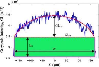
Figure 7: Example fluorescent microscopy measurement of the bulging of a microchannel’s cross-section in the $(x,y)$ plane at fixed axial location $z$ (out of the page). The noisy curve is the measurement, and a normalized, filtered grayscale intensity (GI) is calibrated and mapped to a deformed channel height $h(x,z)$. Reprinted by permission from Springer Nature’s Microfluid. Nanofluid. [118] © 2017.

3.5 Deformation–pressure relations

Flow conduits manufactured from soft polymeric materials deform due to the transmural pressure difference caused by the flow within [17, 72], bulging out when the external pressure is lower than the internal one. When dealing with complex fluids and a PDMS-based elastomer, care must be taken that the PDMS does not uptake fluid (such as a mineral oil for which it has affinity) from the channel, because such infiltration can lower the PDMS’ Young’s modulus by a factor of two over the course of hours [119]. Figure 7 shows an example fluorescence microscopy measurement of the deformation of an initially rectangular cross-section of a microchannel due to the flow within it.

Under the theory of linear elasticity, the deformation $u_{y}(z)$ (or $u_{r}(z)$) is expected to be proportional to $p(z)$ scaled by geometric factors ($a$, $t$, $h_{0}$, etc.) and elasticity constants (table 3) [120]. Conventionally, the strain ($u_{y}(z)/h_{0}$ or $u_{r}(z)/a$) is taken to be $\propto p(z)/E$ (see, e.g., [17]). The idea is that the proportionality constant can be calibrated from experiments [17, 72]. However, a predictive model requires calculating the proportionality constant from the governing equations of elasticity. After initial attempts [54, 118], our current understanding has settled on a set of canonical relations, illustrated in figure 8, between $u_{y}(z)/h_{0}$ (or $u_{r}(z)/a$) and $p(z)/E$, with the proportionality factor having been determined by solving a suitable elasticity problem. Importantly, this observation that the deformation at any fixed-$z$ cross-section depends only on the local hydrodynamic pressure $p(z)$, while the axial bending and tension (as well as the fluid shear stresses) are negligible, has been justified by perturbation methods [101, 109, 117, 110, 107] within the long-and-shallow-conduit scaling that leads to the lubrication approximation.

Table 3: Elasticity constants and their interrelations. Typical values are quoted in the main text.

Quantity	Notation	Units	Definition
Young’s modulus	$E$	Pa	–
Poisson ratio	$\nu$	–	–
Plane-strain $E$	$\overline{E}$	Pa	$\frac{E}{(1-\nu^{2})}$
Shear modulus	$G$	Pa	$\frac{E}{2(1+\nu)}$
First Lamé parameter	$\lambda$	Pa	$\frac{E\nu}{(1+\nu)(1-2\nu)}$
Compliance	$\mathcal{C}$	m/Pa	$\frac{t}{2G+\lambda}$, $\frac{a}{4G}$, $\frac{a^{2}}{t\overline{E}}$, $\frac{\alpha w}{\overline{E}}$
			(context dependent)

Thus, unlike rigid pipes (figure 5), calculating the hydraulic resistance of a soft conduit requires the solution of a non-trivial elasticity problem (figure 8), in addition to the flow problem. Depending on the conduit geometry, the balance of elastic forces can be entirely different. Example mathematical expressions for the function $\mathfrak{G}(p,\mathrm{d}p/\mathrm{d}z)$ can be “read off” from the equations in sections 3.4.1 and 3.4.2. However, these expressions depend on $p$ implicitly through the tube radius $R$ (deformed from $a$) and channel height $h$ (deformed from $h_{0}$). To fully specify $\mathfrak{G}$, suitable deformation–pressure relationships must be determined. Figure 8 shows four geometries that can be analyzed by the perturbative approach:

• 2D planar configuration with vertical deformation [121, 122, 123]:

  $$h=h(z)=h_{0}+u_{y}(z),$$ (27)

  $$u_{y}(z)=t\frac{p(z)}{2G+\lambda}.$$ (28)

• 3D axisymmetric exclusion, within an infinite elastic medium, with radial deformation [124]:

  $$R=R(z)=a+u_{r}(z),$$ (29)

  $$u_{r}(z)=\frac{a}{4}\frac{p(z)}{G}.$$ (30)

• 3D axisymmetric thin shell with radial deformation [110, 107]:

  $$R=R(z)=a+u_{r}(z),$$ (31)

  $$u_{r}(z)=\frac{a^{2}}{t}\frac{p(z)}{\overline{E}}.$$ (32)

• 3D Cartesian configuration (thick or thin) with vertical deformation [101, 115, 109, 117]:

  $$h=h(x,z)=h_{0}+u_{y}(x,z),$$ (33)

  $$u_{y}(x,z)=F(x)\frac{p(z)}{\overline{E}},$$ (34)

  for some $F(x)$ determined from linear elasticity.

Note that case (d) is unconfined on top, unlike (a). However, it was shown by Wang and Christov [109] that the vertical displacement decays exponentially with vertical distance from the fluid–solid interface for a thick elastic top wall. Further, the result in case (d) requires the use of the shallowness assumption of the microchannel ($h_{0}\ll w$). For cross-sections that are close to square ($h_{0}\sim w$) techniques based on conformal mappings [125] could potentially be employed to obtain the deformation from the equations of linear elasticity. However, this approach has not yet been coupled to flow (via the hydrodynamic pressure $p(z)$).

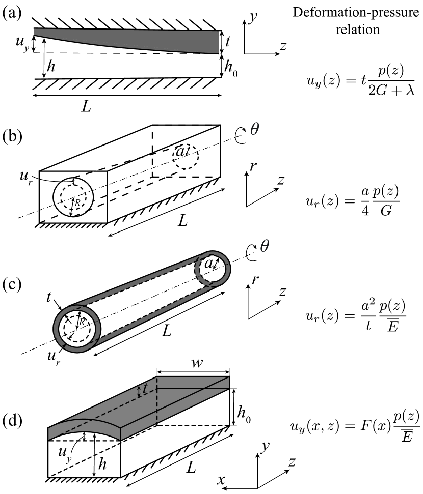
Figure 8: Building blocks for soft hydraulic resistance calculations. Four model geometries are shown schematically in which the flow-induced deformation can be analyzed mathematically, yielding a fitting-parameter-free deformation–pressure relationship.

It should also be emphasized that these relationships rest on the result from lubrication theory that the pressure varies only in the flow-wise direction, i.e., $p=p(z)$, for a long and slender conduit (as in figure 8) [49]. The most challenging case is the 3D microchannel in figure 8(d), for which the expression for the function $F(x)$ depends on whether the rectangular wall is thin (i.e., plate theory applies [101, 115]) or thick (i.e., the “full” equations of linear elasticity must be employed [109]). Recently, it has been shown [126] that spanwise-averaging the deformation as

$$\langle u_{y}\rangle_{x}(z)=\int_{-w/2}^{+w/2}u_{y}(x,z)\,\mathrm{d}x=\alpha w\frac{p(z)}{\overline{E}},$$ (35)

where $\alpha=\int_{-1/2}^{+1/2}F(x/w)\,\mathrm{d}(x/w)$ is dimensionless, commits only a small error in the final solution to the coupled problem. Although this result was established for Newtonian fluids, its generalization to non-Newtonian fluids is highlighted below. The constant $\alpha$ has been calculated from theory (no fitting or calibration required) [126] as

$$\alpha=\left\{\begin{array}[]{@{}l@{\quad}l}\frac{1}{60}\left(\frac{w}{t}\right)^{3}\left[1+\frac{10(t/w)^{2}}{\varkappa(1-\nu)}\right]&\quad(\mathrm{plate}),\\[5.69054pt] 0.542742&\quad(\mathrm{halfspace}).\end{array}\right.$$ (36)

The “plate” case considers thick-plates $t/w<1$ (but not necessarily restricted to $t/w\ll 1$), $\varkappa$ is a shear-correction factor taken to be unity [115]. The “halfspace” case refers to the limit $t^{2}/w^{2}\to 0$, in which the wall thickness drops out [109].

Importantly, the span-averaged deformation–pressure relation (35) allows us to treat the 3D channel geometry in figure 8(d) in the same way as those in figure 8(a,b,c). Then, all the local deformation–pressure relations reviewed here resemble a Winkler “mattress” foundation [127, 128] with $p=k_{w}u_{y}$ (or $p=k_{w}u_{r}$). The effective stiffness $k_{w}$ can be obtained from the expressions in figure 8. For convenience, the compliance $\mathcal{C}=1/k_{w}$ is now introduced. Here, $\mathcal{C}$ is not to be confused with the hydraulic capacitance, which also arises from compliance, within the hydraulic–electric circuit analogy [49, section 4.6]. Capacitance will not be discussed in this review.

3.6 Analytical models for the coupled problem and their solution

Combing the physics of the flow reviewed in section 3.4 with the physics of the flow-induced deformation reviewed in section 3.5, yields the basic laws of soft hydraulics. Specifically, these laws will take the form of nonlinear ODEs for the hydrodynamic pressure $p(z)$, from which the deformation and velocity field can be reconstituted.

3.6.1 Microtubes/micropipes

For the geometries in figure 8(b,c), (23) becomes:

$$-\frac{\mathrm{d}p}{\mathrm{d}z}=\frac{2(3+1/n)^{n}Kq^{n}}{\pi^{n}[a+\mathcal{C}p(z)]^{1+3n}},$$ (37)

where $\mathrm{d}p/\mathrm{d}z<0$ so that $|\mathrm{d}p/\mathrm{d}z|=-\mathrm{d}p/\mathrm{d}z$ for flow in the $+z$-direction. Here, $\mathcal{C}=a/(4G)$ for the cylindrical exclusion geometry (“micropipe,” figure 8(b)), while $\mathcal{C}=a^{2}/(t\overline{E})$ for the cylindrical shell (“microtube,” figure 8(c)). A typical cylindrical exclusion in PDMS has $\mathcal{C}\approx 0.3$ $\mu$m/kPa (experimental fit), with values up to 4 $\mu$m/kPa possible when using silicone rubbers like “Dragon Skin” [129]. Equation (37) can be solved as a separable first-order ODE to obtain [107]:

$$p(z)=\frac{a}{\mathcal{C}}\left\{\left[1+\hat{n}_{t}\left(\frac{\mathcal{C}KLq^{n}}{\pi^{n}a^{2+3n}}\right)\left(1-\frac{z}{L}\right)\right]^{\frac{1}{2+3n}}-1\right\},$$

(38)

where $\hat{n}_{t}=2(3+1/n)^{n}(2+3n)$ for convenience.

A non-trivial dimensionless group, which is interpreted as the fluid–structure interaction parameter $\beta$ [101], arises from this calculation:

$$\eqalign{\beta&=\frac{\mathcal{C}KLq^{n}}{\pi^{n}a^{2+3n}}=\frac{KL\langle v_{z}\rangle^{n}/a^{1+n}}{a/\mathcal{C}}\\ &\simeq\frac{\mathrm{hydrodynamic~{}forces~{}on~{}wall}}{\mathrm{elastic~{}resistance~{}of~{}wall}}.}$$ (39)

Here, $\langle v_{z}\rangle=q/(\pi a^{2})$. By balancing (14) with the power-law model (4) for the viscosity, $\mathscr{P}_{c}=KL\langle v_{z}\rangle^{n}/a^{1+n}$ can be shown to be the characteristic pressure scale (hydrodynamic force per area) for this flow. It follows that $\mathscr{U}_{c}=\beta a=\mathscr{P}_{c}\mathcal{C}$ is a characteristic deformation scale.

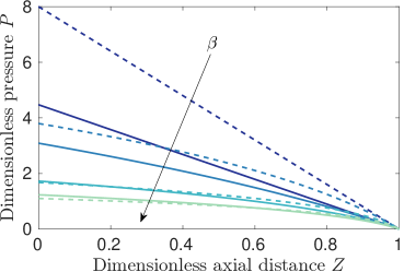
(a)

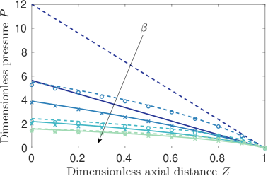
(b)

Figure 9: (a) Dimensionless pressure $P(Z)=p(z)/\mathscr{P}_{c}$ variation along a compliant microtube/micropipe ($Z=z/L$) for a Newtonian fluid (38) with $n=1$ (-  -  -  -) and a shear-thinning fluid (38) with $n=0.5$ (——). (b) Dimensionless pressure $P(Z)=p(z)/\mathscr{P}_{c}$ variation along a compliant microchannel ($Z=z/L$) for a Newtonian fluid (41) with $n=1$ (-  -  -  -) and a shear-thinning fluid (41) with $n=0.5$ (——). Symbols show the corresponding ($\opencircle$, $n=1$) and ($\times$, $n=0.5$) pressure profiles found from numerically integrating the “full” microchannel theory (3.6.3). In both cases, a thin plate compliant top wall, with negligible $(t/w)^{2}/[\varkappa(1-\nu)]$, is considered. Colors represent different values of the fluid–structure interaction parameter $\beta=0,0.1,0.5,1$ (top to bottom, dark to light). Note that $\mathscr{P}_{c}$ and $\beta$ are context-dependent and defined differently for (a) and (b), as discussed in the text.

3.6.2 Microchannels: span-averaged theory

For the geometry in figure 8(d) and using (35), (25) becomes:

$$-\frac{\mathrm{d}p}{\mathrm{d}{z}}=\frac{2^{1+n}(2+1/n)^{n}Kq^{n}}{[h_{0}+\mathcal{C}p(z)]^{1+2n}w^{n}},$$ (40)

where $\mathcal{C}=\alpha w/\overline{E}$ with $\alpha$ given in (36) for a flow conduit with Cartesian geometry. A typical microchannel with a thin deformable membrane as its top wall has $\mathcal{C}\approx 1-10$ $\mu$m/kPa (experimental fit) [130]. Equation (40) can be solved as a separable first-order ODE to obtain:

$$p(z)=\frac{h_{0}}{\mathcal{C}}\left\{\left[1+\hat{n}_{c}\left(\frac{\mathcal{C}KLq^{n}}{h_{0}^{2+2n}w^{n}}\right)\left(1-\frac{z}{L}\right)\right]^{\frac{1}{2+2n}}-1\right\},$$

(41)

where $\hat{n}_{c}=2^{1+n}(2+1/n)^{n}(2+2n)$ for convenience. Once again, a fluid–structure interaction dimensionless parameter emerges from (41):

$$\beta=\frac{\mathcal{C}KLq^{n}}{h_{0}^{2+2n}w^{n}}=\frac{KL\langle v_{z}\rangle^{n}/h_{0}^{1+n}}{\overline{E}h_{0}/(\alpha w)}.$$ (42)

Here, $\langle v_{z}\rangle=q/(h_{0}w)$, and $\mathscr{P}_{c}=KL\langle v_{z}\rangle^{n}/h_{0}^{1+n}$ can be shown to the be characteristic pressure scale for this flow [53]. It follows that $\mathscr{U}_{c}=\beta h_{0}=\mathscr{P}_{c}\mathcal{C}$ is a characteristic deformation scale.

To estimate a typical value of $\beta$ for a non-Newtonian soft hydraulic system, consider the typical compliant ($\overline{E}\approx 1$ MPa, $\alpha\approx 1$), long and shallow microchannel ($h_{0}\approx 25$ $\mu$m, $w\approx 10h_{0}$, $L\approx 100h_{0}$) [17]. For the power-law model’s parameters used in figure 6 ($K\approx 1.25$ Pa$\cdot$sⁿ, $n\approx 0.41$) and a flow at $\langle v_{z}\rangle\approx 1$ m/s (for $q\approx 300$ $\mu$L/s [17]), yields $\beta\approx 0.1$. Importantly, however, the theory reviewed above does not require $\beta\ll 1$, and it is applicable up to $\beta=\mathcal{O}(1)$ [101, 109].

3.6.3 Microchannels: “full” theory

Without using the spanwise-averaging idea to reduce $u_{y}(x,z)$ to a function of $z$ alone, the coupled two-way fluid–structure interaction problem can still be reduced to single nonlinear ODE for $p(z)$. To understand the challenges in using the “full” theory of the 3D Cartesian geometry’s deformation, consider (17), which becomes:

$$q=\int_{-w/2}^{+w/2}\!\!\int_{0}^{h_{0}+u_{y}(x,z)}v_{z}\,\mathrm{d}x\,\mathrm{d}y.$$ (43)

Therefore, (25) becomes

$$\eqalign{-\frac{\mathrm{d}p}{\mathrm{d}z}\left[\frac{1}{2^{1+1/n}(2+1/n)K^{1/n}}\left|\frac{\mathrm{d}p}{\mathrm{d}{z}}\right|^{(1/n)-1}\right]\\ \qquad\times\int_{-w/2}^{+w/2}[h_{0}+u_{y}(x,z)]^{2+1/n}\,\mathrm{d}x=q.}$$ (44)

The last integral is to be evaluated using a suitable deformation–pressure relationship, such as $u_{y}(x,z)=F(x)p(z)/\overline{E}$. However, this integral does not always yield a closed-form expression due to the fractional power $2+1/n$ involved.

Anand et al. [53] used a generalized binomial expansion to handle the latter difficulty, and finally obtained the desired ODE for $p(z)$:

$$-\frac{\mathrm{d}p}{\mathrm{d}z}=\frac{Kq^{n}}{h_{0}^{1+2n}w^{n}}{2^{1+2n}(2+1/n)^{n}}\pi^{-n/2}$$

$$\times\Bigg{[}\sum_{k=0}^{\infty}C_{k,n}\Bigg{\{}\frac{1}{2^{5}}\frac{w}{\overline{E}h_{0}}\frac{w^{3}}{t^{3}}\left[1+\frac{8(t/w)^{2}}{\varkappa(1-\nu)}\right]p(z)\Bigg{\}}^{k}$$

$$\quad\times\,\Gamma{(k+1)}\,{}_{2}\tilde{F}_{1}\Bigg{(}\frac{1}{2},-k;\frac{3}{2}+k;\frac{1}{1+\frac{8(t/w)^{2}}{\varkappa(1-\nu)}}\Bigg{)}\Bigg{]}^{-n},$$ (45)

where ${}_{2}\tilde{F}_{1}$ is the regularized hypergeometric function, $\Gamma$ is the gamma function,

$$C_{k,n}=\frac{\Gamma(3+1/n)}{\Gamma(k+1)\Gamma(3-k+1/n)}$$ (46)

are binomial-like coefficients, and $\varkappa$ is again a shear correction factor taken to be unity. Once the pressure $p(z)$ is determined via (3.6.3), the deformed channel shape can be found as $h(x,z)=h_{0}+F(x)p(z)/\overline{E}$ (recall figure 8). An example Python code for solving this ODE numerically is available in the supplementary material associated with [53].

To illustrate and summarize the basic results on the pressure distribution in a soft hydraulic conduit, figure 9 shows the dimensionless pressure $p(z)/\mathscr{P}_{c}$ variation along the compliant microchannel, i.e., against dimensionless axial distance $z/L$, for both Newtonian and non-Newtonian fluids and different values of the dimensionless fluid–structure interaction parameter $\beta\propto\Delta p/E$. Both the shear-thinning rheology and fluid–structure interaction decrease the pressure drop, which is evaluated from $p(0)$. For $\beta=\mathcal{O}(1)$, it is interesting to note that all the profiles saturate, showing that the strongest effect of the interaction between the non-Newtonian fluid’s rheology and the compliance of the conduit is for small $\beta$, which is typical in practice. This observation has implications for the sensitivity of microfluidic rheological measurements (see section 4.1). In figure 9(b), observe also that (41) (curves) is a good approximation to $p(z)$ found by solving the nonlinear ODE (3.6.3) (symbols).

The reference pressure distributions for Newtonian flow in a rigid conduit ($n=1$ and $\beta=0$) are (a) $p(z)/\mathscr{P}_{c}=8(1-z/L)$ and (b) $p(z)/\mathscr{P}_{c}=12(1-z/L)$, which can be obtained by a Taylor series expansion in $\beta\ll 1$ (or a limit using L’Hôpital’s rule) from (38) and (41), respectively.

3.6.4 Special case: flow rate–pressure drop relations

Whenever the ODE governing the coupled soft hydraulics problem can be solved analytically for $p(z)$, subject to gauge outlet pressure $p(L)=0$, the relationship between the pressure drop $\Delta p=p(0)-p(L)$ and the steady volumetric flow rate $q$ can be obtained, as suggested by (22). When (22) can be resolved algebraically as $\Delta p=R_{h}(\Delta p)q$ or as $q=\Delta p/R_{h}(q)$, the tunable soft hydraulic resistance $R_{h}(\Delta p)$ or $R_{h}(q)$ can be determined.

From the two prototypical pressure distributions for non-Newtonian fluid flow in a soft hydraulic conduit, namely (38) for the microtube/micropipe and (41) for the microchannel, it is trivial to evaluate $\Delta p$ in each case. However the resulting expressions cannot be algebraically resolved as $\Delta p=R_{h}q$, unless an expansion in $\beta\ll 1$ is performed. However, these flow rate–pressure drop relations can, of course, be easily inverted numerically. In fact, an implicit relation of the form (22) can also be obtained under the Carreau model (5) [131] (but note that the validity of the variational method used for validation in [131] has been questioned [132]). Most recently, Boyko and Stone [133] obtained explicit analytical results for small, intermediate and large Carreau numbers [$\lambda_{r}\Delta ph_{0}/(\eta_{0}L)$] via perturbation methods.

Similarly, the “full” microchannel result (3.6.3) does not allow for an analytical evaluation of $\Delta p$. However, its Newtonian counterpart ($n=1$, $K=\eta_{0}$) does, and yields:

$$\Delta p=\underbrace{\overbrace{\frac{12\eta_{0}L}{h_{0}^{3}w}}^{\mathrm{rigid~{}channel}}\left[\sum_{k=0}^{3}\left(\frac{w}{\overline{E}h_{0}}\right)^{k}S_{k}(\Delta p)^{k}\right]^{-1}}_{\mathrm{Newtonian~{}soft~{}hydraulic~{}resistance,~{}}R_{h}(\Delta p)}q,$$ (47)

the parameters $S_{1}$, $S_{2}$ and $S_{3}$ are known functions of the geometry (e.g., wall thickness $t$) [115, 109], or potentially pre-stress in the wall [117]. The term outside of the bracket can be compared to figure 5 (row “two plates”).

Equation (47) is an analytical result capturing the tunable nonlinear resistance [71, 70] of a soft hydraulic conduit. This expression is not a perturbation series in $\Delta p$. The dependence of $S_{1}$, $S_{2}$ and $S_{3}$ on geometry (and even pre-stress) enables tuning of the nonlinear resistance. Using this approach, the ultra-low aspect ratio regime ($w/h_{0}\gg 1$) was studied experimentally by Mehboudi and Yeom [134], highlighting the (perhaps unexpected) importance of the higher powers of $\Delta p$ in (47), which are dominant in this regime. It would be of interest to further develop these concepts for non-Newtonian flows in compliant conduits.

4 Maturing applications areas

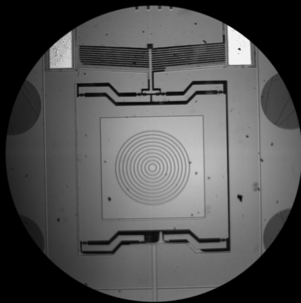
Figure 10: A MEMS-based dynamic shear microrheometer (“MEMS-$\mu$R”) [135, 136]. The chip shown is a few millimeters in width and height, with the central square region, where the fluid sample is placed, being $\approx 500$ $\mu$m. Oscillatory shear is generated by the “chevron-like structure” at the top of the chip. The nested beams in the chevron are actuated by resistance heating elements (contact pads to the left and right), which in turn sets the central stage into motion. The gap thickness into the page is $\approx 10$ $\mu$m. The chip can be placed in an optical microscope to detect the motion of and flow within the sample using a high-speed camera. From the latter optical measurement, the rheological parameters of the material can be estimated. The MEMS-$\mu$R uses only $5$ nL of material. Reproduced from [136], photo credit: G. Christopher/NIST, by courtesy of the National Institute of Standards and Technology. All rights reserved, U.S. Secretary of Commerce.

4.1 Microfluidic rheometry

It has been proposed that rheological measurements can also be performed with miniaturized setups, involving small amounts of liquid (obviating the need for multiple dilutions) and improved optical measurement capabilities (via microscopy) [82]. Utilizing flows in microchannels gives rise to microfluidic rheometry [137, 138] also known as “rheometry-on-a-chip” [139]. An example of such a (rigid) chip, designed and manufactured by the US National Institute of Standards and Technology (NIST), is shown in figure 10. Srivastava and Burns [140] microfabricated a transient capillary viscometer capable of measuring $n$ for the power-law non-Newtonian model (4) in $2$–$8$ min from 1 $\mu$L of fluid. More generally, microfluidic rheometry enables the characterization of low-viscosity fluids [141] and the measurement of the relaxation time of weakly-elastic fluids down to milliseconds [139], both of which are normally challenging using macroscopic rheometers. In the biopharamaceutical industry, it is desirable to perform rheological measurements not only using a small-volume samples of fluid, but also across a significant range of shear rates, and without interaction between the sample and air (such as at a free surface). A microrheometer fits the bill [142]. Another benefit of miniaturization is the ability to easily generate high-frequency flows [143] in PDMS-based microchannels and induce acoustic streaming [144, 145] past a cylindrical pillar in the channel. Oscillatory-flow techniques are not only useful for measuring the shear viscosity of low-viscosity liquids [146], but also for characterizing the storage and loss moduli and relaxation time of viscoelastic dilute and semi-dilute polymeric solutions [147].

In the most basic form of microrheometry, experiments that characterize the pressure drop for a given flow rate are compared to a theoretical prediction. The flow rate–pressure drop curve (recall section 3.6.4) is a cornerstone of capillary viscometry, even for non-Newtonian fluids [79, chapter 2]. The shear-rate-dependent viscosity of non-Newtonian fluids can be taken into account, yielding correlations [148] from which the steady shear viscosity and its rate dependence can be inferred from simultaneous measurements of $\Delta p$ and $q$. Essentially, these approaches rely on a correlation for the friction factor, which is a dimensionless pressure drop (Darcy–Weisbach friction factor):

$$f_{D}=\frac{\Delta p/L}{\frac{1}{2}\rho\mathscr{V}_{c}^{2}/D_{h}},$$ (48)

Equations such as (48) are key to microfluidic system design [149], much like their use for analyzing industrial pipe networks [85, chapter 8], including non-Newtonian ones [79, section 3.8]. The friction factor allows for a convenient parametrization of viscous (energy) losses in both laminar and turbulent flows [85]. In (48), $\mathscr{V}_{c}$ is suitable velocity scale, e.g., $\langle v_{z}\rangle$; $D_{h}$ is a suitable hydraulic diameter, e.g., $4\mathcal{A}/\mathcal{P}$, where $\mathcal{A}$ and $\mathcal{P}$ are the area and perimeter of an axial cross-section of the flow conduit, respectively. Typically, the same $\mathscr{V}_{c}$ and $D_{h}$ are substituted for $\mathscr{V}_{c}$ and $h_{0}$ in (11) to define the appropriate Reynolds number for the flow.

If the pressure drop is not know a priori, it is more convenient to define the friction factor as a dimensionless (local) mean wall shear stress $\bar{\tau}_{w}$ (Fanning friction factor) [148, 149]:

$$f_{F} = \frac{\bar{\tau}_{w}}{\frac{1}{2}\rho\mathscr{V}_{c}^{2}},$$ (49)

$$\bar{\tau}_{w} = \frac{1}{\mathcal{P}}\oint_{\mathcal{P}}\tau_{w}\,\mathrm{d}\ell=\frac{D_{h}}{4}\left(-\frac{\mathrm{d}p}{\mathrm{d}z}\right),$$ (50)

where $\tau_{w}$ is the shear stress evaluated at the wall. Under these definitions, $f_{F}=f_{D}/4$ [149], but care must be taken to properly relate $\bar{\tau}_{w}$, $\Delta p$ and $\mathscr{V}_{c}$ in a non-Newtonian flow via the momentum equation (14). For example, for a power-law fluid one can define a generalized Reynolds number $Re_{g}$ and obtain [148] (see also [79, chapter 3]):

$$f_{F} = \frac{16}{Re_{g}},$$ (51)

$$Re_{g} = \frac{\rho\mathscr{V}_{c}^{2-n}D_{h}^{n}}{8^{n-1}(c_{2}+c_{1}/n)^{n}K},$$ (52)

which is also valid for a Newtonian fluid ($n=1$, $K=\eta_{0}$). In (51), $c_{1}$ and $c_{2}$ are the so-called Rabinowitsch–Mooney constants depending on the flow conduit’s geometry. For a circular pipe, $c_{1}=1/4$ and $c_{2}=3/4$; for a parallel plate channel, $c_{1}=1/2$ and $c_{2}=1$ [148]. Observe that, from (51), the Poiseuille number $Po=f_{F}Re_{g}$ is a constant determined solely by the cross-sectional shape of the (rigid) conduit [68, 149].

The goal of using $Re_{g}$ is to eliminate ambiguities and challenges that arise due to the different shear rates experienced by fluids in microchannels of different shapes [150]. Then, for example, given experimental measurements of $f_{F}$, the power-law rheological parameters $K$ and/or $n$ can be back-calculated from (51) via (52). Clearly, an accurate friction factor theory of non-Newtonian flow in microfluidic conduits is key to microrheometry. However, beyond the (51)–(52) for the power-law model, few similar parametrizations exist for other shear-dependent viscosity models. It is of interest to develop such relations because the power-law model is only applicable over some intermediate range of shear rates (recall figure 6(c)), failing to capture the high-shear Newtonian plateau (for $\dot{\gamma}_{c}\sim 10^{4}-10^{6}$ s^-1) now being accessed using microrheometers [151, 152] (see also the discussion in [133]).

The MEMS-based dynamic shear microrheometer shown in figure 10 uses glass plates to confine the sample. It can be easier and cheaper to manufacture the confined channels from, e.g., PDMS using soft lithography. However, given that PDMS-based microchannels are compliant, an open problem in microrheology [56] is whether such measurements are affected by the dependence $\propto\Delta p/E$ introduced by fluid–structure interaction (recall section 3.5). Taking this idea one step further, Shiba et al. [153] exploited compliance to measure the viscosity of Newtonian fluids (both liquids and gases). They used a strain gauge to quantify a PDMS microchannel’s flow-induced deformation, then calibrated the strain–viscosity relationship empirically.

Recently, Wang and Christov [126] addressed the $\Delta p/E$ dependence of the friction factor for Newtonian fluid flow through a soft hydraulic conduit. Implementing their derivation for the power-law fluid through a microchannel (a microtube can be handled analogously), one first needs to account for the flow-induced conduit deformation in the expressions for $\mathscr{V}_{c}$ in (49) and $D_{h}$ in (50), replacing them by local expressions:

$$\mathscr{V}_{c} = q/[h_{0}(1+\mathcal{C}p/h_{0})w]=\mathscr{V}_{c,h_{0}}/(1+\mathcal{C}p/h_{0}),$$ (53)

$$D_{h} = D_{h_{0}}(1+2\mathcal{C}p/h_{0}).$$ (54)

In (53), $\mathscr{V}_{c,h_{0}}=q/(h_{0}w)$ is the mean axial velocity in the undeformed channel and $D_{h_{0}}=4h_{0}w/[2(h_{0}+w)]$ in (54) is its hydraulic diameter. To arrive at (54), the force balance used to evaluate (50) had to be rederived for a compliant flow conduit [126]. Then, combining (49), (50) and (40) yields

$$f_{F} = \frac{(1+\mathcal{C}p/h_{0})^{2}}{\frac{1}{2}\rho\mathscr{V}_{c,h_{0}}^{2}}\frac{D_{h_{0}}(1+2\mathcal{C}p/h_{0})}{4}$$ (55)

$$\times\frac{2^{1+n}K(2+1/n)^{n}q^{n}}{h_{0}^{1+2n}(1+\mathcal{C}p/h_{0})^{1+2n}w^{n}}$$

$$= \frac{D_{h_{0}}^{1+n}}{h^{1+n}}\frac{2^{2n}[1+1/(2n)]^{n}K}{\rho\mathscr{V}_{c,h_{0}}^{2-n}D_{h_{0}}^{n}}\frac{(1+2\mathcal{C}p/h_{0})}{(1+\mathcal{C}p/h_{0})^{2n-1}}.$$

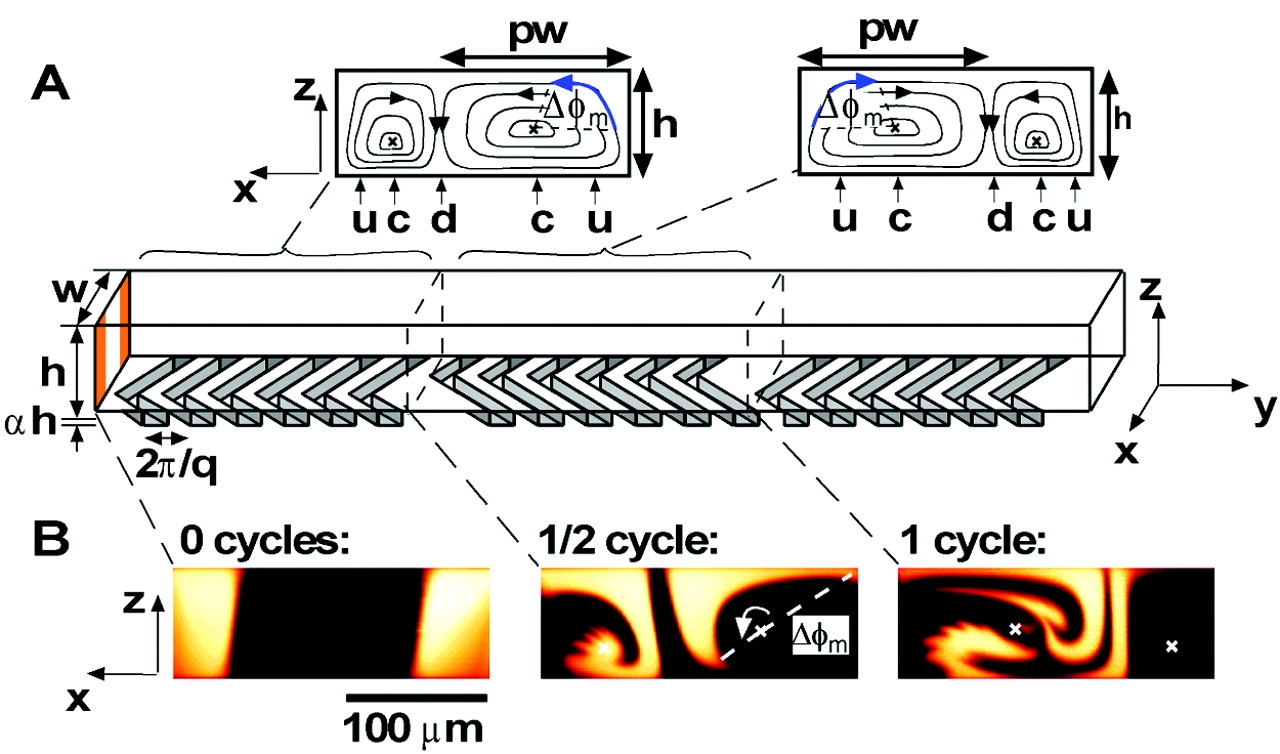
(a)

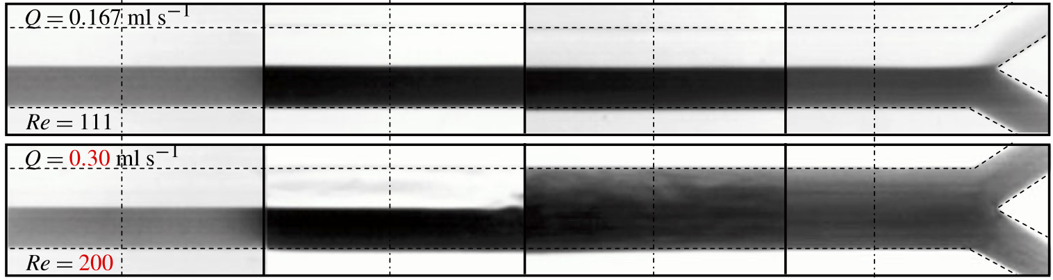
(b)

Figure 11: (a) Staggered herringbone mixer (SHM); subpanel A shows the periodic pattern on the lower channel wall (rigid) and resulting secondary flows, while subpanel B shows conformal micrographs of the mixing of dyes in the channel at $Re\approx 0$. From Stroock et al. 2002 Science 295 647–651 [154]. Reprinted with permission from AAAS. (b) Instability leads to mixing in a soft-walled microchannel flow, without patterning the wall but, rather, due to fluid–structure interaction at an unusually low, but finite, $Re\neq 0$. The channel is manufactured from a PDMS-based elastomer to yield a low shear modulus $G\approx 10-50$ kPa. Reproduced from [155] with permission from Cambridge University Press © 2013. An optical visualization is shown, in the style of Reynolds’ dye breakup experiment [103], at four representative (non-continuous) segments of the long microchannel. The working fluid in (b) is water, however the same flow–structure instability is observed with dilute polymeric solutions [156, 157]. In both panels, the flow is left to right.

Next, observing that $[1+1/(2n)]^{n}=(c_{2}+c_{1}/n)^{n}$ for a microchannel and $D_{h_{0}}/h_{0}=2/(1+h_{0}/w)\simeq 2$ for $h_{0}\ll w$, one can introduce the definition of $Re_{g}$ (based on $D_{h_{0}}$ and denoted $Re_{g,h_{0}}$) from (52) into (55) to obtain:

$$f_{F}=\frac{16}{Re_{g,h_{0}}}\frac{(1+2\mathcal{C}p/h_{0})}{(1+\mathcal{C}p/h_{0})^{2n-1}}.$$ (56)

Then, from (53) and (54), the generalized Reynolds number for the deformed channel is

$$Re_{g}=Re_{g,h_{0}}\frac{(1+2\mathcal{C}p/h_{0})^{n}}{(1+\mathcal{C}p/h_{0})^{2-n}}.$$ (57)

Finally, the Poiseuille number for the flow of a non-Newtonian fluid under the power-law model in a deformable microchannel is obtained from (56) and (57):

$$Po=f_{F}Re_{g}=16\left(1+\frac{\mathcal{C}p}{h_{0}+\mathcal{C}p}\right)^{n+1}.$$ (58)

Equation (58) highlights that compliance alone can increase $Po$ by up to a factor of $2^{n+1}$ (for $\mathcal{C}p\gg h_{0}$), which is not negligible. Note that $p=p(z)$ in (58) is given by (41). Due to the flow-induced deformation, the Poiseuille number now varies axially.

4.2 Microfluidic mixing

Fast and efficient mixing of fluids in labs-on-a-chip is of tremendous technological importance: micro total analysis systems ($\mu$TAS) [158, 159], which have enabled low-cost disposable medical diagnostics [160, 161] with public health implications [162], rely on reagents and biological fluid samples mixing and reacting thoroughly. However, “[t]he design and implementation of mixers in microfluidics differs considerably from that on the macroscale” [163]. At the macroscale, the laminar–turbulent transition enables efficient mixing, which Osborne Reynolds [103] used to visualize the instability. Meanwhile, at the microscale, flows are dominated by viscosity and mixing is limited by diffusion. For a Newtonian fluid, G. I. Taylor demonstrated, in a classic film [164], the well-known kinematic reversibility of Stokes flow ($Re=0$) . Mixing by molecular diffusion between fluids requires channel lengths of 0.1 to 1 meters [165, 163]. For example, the diffusivity of hemoglobin into water is $\kappa\simeq 70$ $\mu$m²/s [51, section 9.1]. The diffusion time across a microchannel of height $h_{0}\approx 25$ $\mu$m is $t_{D}=h_{0}^{2}/\kappa\approx 9$ s. During this time, for the typical flow speed of $\mathscr{V}_{c}=4\times 10^{-2}$ m/s quoted in section 3.3, a fluid parcel would have traveled a distance $\mathscr{V}_{c}t_{D}\approx 0.4$ m. Relying on diffusive mixing over such lengths is not always feasible for a lab-on-a-chip processing blood.

In stark contrast to the laminar–turbulent transition, reversibility hinders mixing in microfluidics (“micromixing”), as there is no way to introduce asymmetries in laminar flow in a constant cross-section conduit (see also [25, section 2.4]). To mix, one must “outsmart” kinematic reversibility. Within the present context, one way to do so is to consider viscoelastic fluids. In the flows of such non-Newtonian fluids, purely elastic instabilities can occur even at vanishing Reynolds number (i.e., in the absence of inertia) [166, 167, 168]. Li et al. [169] and Galindo-Rosales et al. [170] reviewed the experimental characterization of these instabilities in rigid microchannels with an outlook towards micromixing (see also [97]).

In the absence of inertia or purely elastic flow instabilities, another approach to circumventing reversibility involves breaking symmetries in the equations governing Lagrangian trajectories, to induce chaotic advection [171, 172]. Static mixer designs based on this principle have uses in the process industry [173, 174]. In microfluidics, patterning the wall of a channel induces secondary flows and chaotic mixing (subpanel A in figure 11(a)) [154]. However, this techniques requires more complex micromanufacturing than just soft lithography.

A third approach is to harness the flow–structure instabilities inherent to soft (e.g., PDMS-based devices). Microchannels manufactured from polymeric materials are soft; consequently, flow–structure instabilities occur, inducing mixing without the need for patterning any channel surfaces (figure 11(b)). First mentioned in the 1970s [175], the application of this discovery did not become clear until Kumaran et al. provided an experimental demonstration of “ultrafast” micromixing (figure 11(b)) in the 2010s [176, 155, 177]. For a Reynolds number $Re=\rho q/(w\eta_{0})$ as low as $\approx 200$, transitional unstable flow is observed. This is in stark contrast with the critical Reynolds number value $Re_{c}\approx 2300$ (for rigid-pipe flow) quoted to undergraduates [85, p. 43] (admittedly an oversimplification [178] but nevertheless valid at the microscale [179]). This new modality of mixing is akin to an active micromixer [180] in which an external force (typically via an acoustic field [181, 182] but, here, via instability) agitates the fluid sample. These instabilities and ultrafast micromixing have also been demonstrated both theoretically [183, 184] and experimentally [156, 157] in non-Newtonian fluid flows of dilute polymeric solutions.

Microfluidics has traditionally resided in the domain of $Re<1$. However, the need to achieve efficient and high-throughput cell sorting has given rise to extreme microfluidics, as Toner terms it in a 2018 Nobel Symposium lecture [185], or nonlinear microfluidics, as Di Carlo terms it in a contemporaneous review [36]. Focusing particles (or cells) in microchannels requires inertia [186, 187]. Current PDMS-based soft microfluidic platforms access the inertial regime up to $Re\simeq 10^{2}$ [188], while epoxy-based “hard” casting allows microflows to achieve $Re\simeq 10^{4}$ [189]. Clearly, the range of $Re$ in which flow–structure instabilities occur is now relevant to current microfluidic technologies. Such instabilities have previously been of interest due to the possibility of the diametrically opposed goal of drag reduction of high-speed flow over hard surfaces via compliant coatings [190, 191]. The complexity of these coatings has not yielded a working theory for applications [68, p. 367], despite a significant amount of research [191, 192] since Kramer’s work on dolphins’ swimming efficiency [193] and Benjamin’s 1960s analysis of linear instabilities [194]. On the other hand, at the microscale where flow-induced deformation is common, ultrafast mixing due to flow–structure instabilities in soft hydraulic conduits has, at least, been conclusively demonstrated [155].

Kumaran et al. [176, 155, 177] characterized the low-Reynolds-number flow–structure instability in compliant conduits. Specifically, their experiments [155] provided support for a scaling $Re_{c}\sim\Sigma^{5/8}$ between the critical Reynolds number $Re_{c}$ at the transition and a dimensionless elastic modulus $\Sigma=\rho GD_{h}^{2}/\eta_{0}^{2}$ (albeit over just a single decade in $\Sigma$). This scaling is “in between” those predicted for instability of inviscid (bulk) modes ($Re_{c}\sim\Sigma^{1/2}$) and viscous (wall) modes ($Re_{c}\sim\Sigma^{3/4}$), both previously identified theoretically for flows in compliant conduits. More recent experiments [195], however, do not quite support this scaling, suggesting a much stronger dependence $Re_{c}\propto\Sigma^{3/2}$ near the transition point. As recently as 2019, inconsistencies have been found in previous calculations [196]. A theoretical re-analysis of a planar Couette flow over a compliant surface of a non-Newtonian fluid under the Carreau model showed that shear-thinning has a strongly stabilizing effect [197], with $Re_{c}\sim\Gamma^{3/(2n-1)}$, where $\Gamma=Gh_{0}/(V_{p}\eta_{0})$ and $V_{p}$ is the velocity of the rigid plate driving the Couette flow. Meanwhile, another experimental study [157] motivated the scaling $Re_{c}\sim El^{-3/2}$, where $El=\lambda_{r}\eta_{0}/(a^{2}\rho)$ is an elasticity number that characterizes the viscoelasticity of the polyacrylamide into water solution used. Therefore, at this time, it appears that a complete understanding and a predictive theory of the instability that enables efficient mixing of non-Newtonian fluids in compliant conduits at low Reynolds numbers is lacking. Nevertheless, the scalings reviewed here reveal that the critical Reynolds number for transition in a compliant conduit is highly tunable using soft materials (such as PDMS with a low shear modulus $G$) and viscoelastic fluids (with sufficiently long relaxation time $\lambda_{r}$). A comprehensive overview/perspective on the problem of stability and transition of flows compliant conduits is available in [198].

5 Advanced topics

5.1 Biomimicry

PDMS is biocompatible, which opens the possibility of both microfluidic analogues of organ functions [23, 24] and the embedding of microfluidic devices and components in vivo [8]. As mentioned in section 1, biological, physiological or even zoological implications of the coupling of flow and compliant boundaries are not topics that are covered in this review, and reader is referred to the reviews in [42, 40, 44, 41] (see also [93, 28] and [25, chapter 8]). Nevertheless, it is worth pointing out a few studies that build upon the concepts reviewed herein.

For example, Kiran Raj et al. [55] suggested that flow of a Xanthan gum solution (a shear-thinning fluid) in a cylindrical pipe embedded in a PDMS block could mimic blood flow in a vein or artery, leading to “biomimetic in-vitro models for lab-on-a-chip applications.” Meanwhile, the non-Newtonian fluid flow in a slender elastic shell considered by Anand and Christov [107] was motivated by the mechanics of a compliant blood vessel sketched out in Fung’s textbook [28] (see also [94]). More recently, Karan et al. [199] reconsidered this type of fluid–structure interaction in the presence of axial gradients in the elastic properties of the compliant wall. This kind of setup can be considered an in vitro model of micro-circulation, in which the gradients in the elastic properties would be due to diseased conditions in vivo. It would be of interest to extend the latter study to non-Newtonian fluid flows.

5.2 Unsteady dynamics

Perhaps the most obvious unsteady problem related to the topics reviewed herein concerns the inflation (or deflation) of a compliant flow conduit due to a suddenly imposed (or ceased) axial pressure drop. This problem has applications to microfluidic stop-flow lithography [200], for which it is important to accurately quantify the time scale of inflation (or deflation) of the microchannel. Dendukuri et al. [200] analyzed this unsteady fluid–structure interaction for the 2D microchannel geometry (figure 8(a)). Mukherjee et al. [201] generalized the latter to electroosmotic flow (see also section 5.3). Elbaz and Gat [110] considered the case of a cylindrical shell geometry (figure 8(c)). Meanhile Martínez-Calvo et al. [202] considered the 3D microchannel geometry (figure 8(d)). These studies focused on characterizing the coupled physics (and parameters) that determine the transient’s time scale, as well as the actual inflation/deflation dynamics. Elbaz et al. [203] additionally analyzed compressible (gas) flow in the 2D microchannel geometry (figure 8(a)), highlighting a variety of self-similar behaviors set by different physical balances. Meanwhile, Anand and Christov [204] considered compressible flow within the cylindrical shell geometry (figure 8(c)) with viscoelastic damping in the structure. They showed that fluid–structure interaction can generate a streaming flow within the compliant conduit.

All these works [200, 201, 110, 203, 202, 204] are restricted to Newtonian working fluids. The basic idea in these papers is to generalize the governing nonlinear ODE (20) for the hydrodynamic pressure $p(z)$ to a nonlinear partial differential equation (PDE) for the unsteady pressure $p(z,t)$. In this subsection, $t$ denotes time, rather than wall thickness. Such a model can be derived by cross-sectionally averaging the governing equations, in which case conservation of mass requires that (see, e.g., [42, 40]):

$$\frac{\partial\mathcal{A}}{\partial t}+\frac{\partial q}{\partial z}=0,$$ (59)

where now $\mathcal{A}=\mathcal{A}(z,t)$ and $q=q(z,t)$ due to unsteady fluid–structure interaction. For a soft hydraulic system, both $\mathcal{A}$ and $q$ can be calculated using the theory reviewed in section 3 and substituted into (59). An example of the end-result of such a calculation is (60) below. These unsteady models, which are one-dimensional (1D), depending only on the axial coordinate $z$, are more complex than the steady models considered in section 3. Nevertheless, the unsteady 1D models can be solved (sometimes analytically) by perturbation [205] and self-similarity methods [206].

A more detailed 1D model, consisting of coupled PDEs for the finite-Reynolds-number lubrication flow (i.e., $Re=\mathcal{O}(1)$ and $\hat{Re}\not\to 0$) of a Newtonian fluid underneath an elastic membrane with inertia, bending and nonlinear stretching (von Kármán strains), was developed by Inamdar et al. [207] and solved numerically. Further, they showed that the inflated shapes of such channels are linearly stable to global perturbations. It is of interest to generalize all these unsteady models to non-Newtonian working fluids. Here, perhaps the most intriguing aspect is the possible breakdown of lubrication theory for a shear-thinning fluid under the power-law model [208], when inertia is included at the leading order in the lubrication theory (as in [207]).

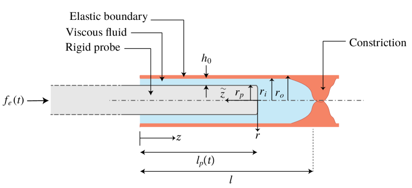
(a)

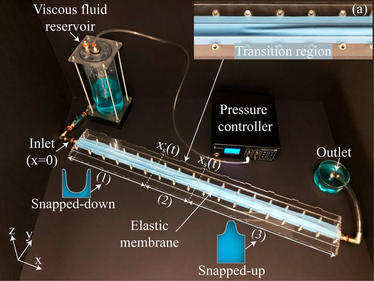
(b)

Figure 12: (a) Schematic of a model of a minimally invasive medical procedure. A rigid cylinder is forced by $f_{e}(t)$ into a fluid-filled elastic tube. The fluid–structure interaction between the flow generated around the cylinder and the attendant elastic deformation sets the intrusion dynamics $l_{p}(t)$. Reproduced from [209] with permission from Cambridge University Press © 2019. (b) Experimental setup used to demonstrate multistability and underactuated fluidic control of an elastic membrane by a low-Reynolds-number viscous channel flow beneath. The working fluid is Newtonian: glycerol with $\rho=1260$ kg/m³ and $\eta_{0}=1.412$ Pa$\cdot$s. A reservoir controls the inlet pressure at $x=0$. A transition region with two fronts, $x_{s}^{\pm}(t)$, slowly moves to the right along the channel and actuates the shape. Reproduced from [210] with permission.

Unsteady fluid–structure interactions also arise during the forced motion of a cylindrical probe into a fluid-filled elastic tube. The latter is a model system for a number of minimally invasive medical procedures such as endoscopies and laparoscopies [209]. As shown in figure 12(a), the motion of the rigid cylinder induces a flow in the gap ($h_{0}=r_{i}-r_{p}$) between itself and the soft wall. The hydrodynamic pressure of this flow can deform the compliant outer wall. The basic equation governing the unsteady dynamics of the insertion or retraction of the rigid cylinder, in the case of a Newtonian fluid, is [209]:

$$\frac{\partial u_{r}}{\partial t}-\frac{1}{12\eta_{0}}\frac{\partial}{\partial z}\left[(h_{0}+u_{r})^{3}\frac{\partial p}{\partial z}\right]+\frac{1}{2}\frac{\partial l_{p}}{\partial t}\frac{\partial u_{r}}{\partial z}=0,$$ (60)

subject to two integral constraints enforcing global conservation of mass and conservation of momentum on the inserted rod. The quantities of interest to be determined in this problem are the radial wall deformation $u_{r}(z,t)$ (or the pressure distribution $p(z,t)$) and the protrusion motion $l_{p}(t)$, given different types of forcing $f_{e}(t)$. Like the results reviewed in section 3, (60) is also based on the lubrication theory of the flow coupled to the equations of linear elasticity for the deformation of the outer wall. The deformation–pressure relation in this case is $u_{r}(z,t)=\frac{r_{i}^{2}}{r_{o}-r_{i}}\frac{p(z,t)}{E}$ [211] (compare to (32)), which can be used to eliminate $u_{r}$ and write (60) as a PDE for $p$.

In another variation on the unsteady dynamics, one considers viscous peeling of the front (e.g., at $z=l_{p}(t)$ in figure 12(a)). Salem et al. [129] successfully leveraged the viscous peeling mechanism for the design of actuators for applications in soft robotics [212]. Importantly, these are multistable systems that lead to “underactuated fluidic control,” which enables patterns to be continuously switched via a single control parameter (e.g., the inlet pressure of the channel) [210]. Peretz et al. [210] demonstrated underactuated control of the multistable shape of soft hydraulic conduits. Their experimental setup is shown in figure 12(b), including a typical pattern of the elastic-walled channel.

To understand the effect of non-Newtonian rheology on unsteady soft hydraulics, Boyko et al. [106] analyzed the flow in a slender elastic tube under the power-law model. As discussed in section 3, the coupling of the nonlinear pressure gradient–flow rate relation for a non-Newtonian fluid with a deformation–pressure relation for the flow-induced deformation can lead to an intractable model. Therefore, a key simplification made in [106] is that the tube’s cross-sectional area does not change significantly, which is akin to linearizing the $(h_{0}+u_{r})^{3}$ term in (60). Then, an unsteady nonlinear PDE governs the pressure evolution in the tube:

$$\eqalign{\frac{\partial p}{\partial t}=\left(\frac{1}{3+1/n}\right)\left[\frac{E(r_{o}-r_{i})r_{i}}{5-4\nu}\right]\frac{\partial}{\partial z}\left[\frac{1}{\tilde{\eta}(\dot{\gamma})}\frac{\partial p}{\partial z}\right],\\ \tilde{\eta}(\dot{\gamma})=\left(\frac{K^{1/n}r_{i}^{1-1/n}}{2^{1-1/n}}\right)\left|\frac{\partial p}{\partial z}\right|^{1-1/n},}$$ (61)

where $r_{i}=a$ is the fluid domain’s (constant) radius, and $r_{o}-r_{i}$ is the thickness of the tube, keeping with the notation from figure 12(a). In (61), the effective viscosity $\tilde{\eta}$ has an “inverse role” compared to the momentum equation (14). Using similarity methods, (61) was solved for a number of unsteady problems, such as an instantaneous injection of mass at the tube’s inlet, sudden change of the inlet pressure, and for the post-transient regime following an oscillatory inlet pressure [106]. Observe that (61) at steady state ($\partial p/\partial t=0$) reduces to (23) (subject to properly defining the flow rate to match), but not to (37) (due to the linearization of the $(h_{0}+u_{r})^{3}$ term).

Similar unsteady problems involving viscous non-Newtonian flows in compliant conduits arise when analyzing the relaxation of an elastic fracture filled with a complex fluid [213, 91]. These types of fluid–structure interactions involving complex fluids are common in hydraulic fracturing [214]. In [213, 91], as a simplification, the deformation is considered to be uniform in the axial direction, so that the channel (fracture) height is just $h(t)$. Then, from (59), a suitable PDE for the non-Newtonian rheology can be derived. The fracture (of length $L$) is considered to have some resistance to opening/proclivity to closing (quantified by a Winkler-like effective stiffness $k_{w}=E/l$, where $l$ is the fracture spacing in the transverse direction). This coupling between flow and elasticity is captured by a global force balance between the hydrodynamic pressure applied on the fracture walls, its elastic properties, and any overload pressure $p_{0}$: $\int_{0}^{L}p(z,t)\,\mathrm{d}z=(E/l)h(t)L+p_{0}L$ [215].

From the results on unsteady soft hydraulics reviewed in this subsection, it is evident that the same basic equations that govern soft hydraulics in microfluidics also allow one to analyze biomedical (minimally invasive surgery) and even geophysical (hydraulic fracturing) problems. The reason for this generality is that the physics (and resultant models) reviewed in section 3 hold across vastly different scales, as long as the basic assumptions (low-Reynolds-number flow, small aspect ratio geometry, lubrication approximation, linearly elastic deformation, etc.) are satisfied.

5.3 Electrohydrodynamics

Electrohydrodynamics, also often referred to as electrokinetics, concerns the flow of electrically conducting fluids. Electric fields cause transport of charged ions within electrolyte solutions. The motion of the ions can “drag” the surrounding fluid, which is perhaps the most striking electrohydrodynamic phenomenon of relevance to microfluidics. The bulk motion (flow), relative to a charged surface, of an electrically conducting fluid due to an imposed electric field is called electroosmosis. Vice versa, a pressure-driven flow of an electrically conducting fluid can lead to the build up of an electrokinetic potential (and, consequently, an electric current in the flow-wise direction), which is called a streaming potential. The standard textbook on this topic is by Probstein [216], while the monograph by Li [217] specifically focuses on electrokinetics in the microfluidics context. Further coverage is available in [1, 3, 49, 29, 30].

Electroosmotic flows are generally “weak” and difficult to realize at the macroscale. Stone et al. [1] estimate that an electric field strength on the order of few kV/cm is needed to achieve flow speeds on the order of mm/s. A high-voltage power supply would be necessary to generate electric fields of this strength in a channel of length of a few cm. Nevertheless, the flow speeds are in the range relevant to microfluidics. A general introduction to electrokinetic actuation of microscale flows is provided by Chakraborty and Chakraborty [218, section 1.4.5], while Ghosal [219] covers the mathematical modeling of charge transport during electroosmotic flows. Alizadeh et al. [220] provide an updated tutorial review on electroosmotic flows in micro- and nanofluidic applications, including a historical overview and discussion of applications of confined flows through micro- and nanoporous media. Electrohydrodynamics is a broad field, and only a few key results related to non-Newtonian flows and flows in compliant conduits are summarized here.

Chakraborty and Chakraborty [221, 123] appear to have been the first to consider the effect of a compliant boundary on the electroosmotic flow of a Newtonian fluid in a narrow confinement, motivated by the phenomenological deformation–pressure relation of Steinberger et al. [222]. Specifically, by analyzing the classical “slider bearing” steady flow problem from lubrication theory, they showed [123] that the load bearing capacity can increase by a factor of up to $\approx 1.5$ under an applied electric field. However, the electrokinetic augmentation effect weakens for highly compliant substrates. Das et al. [223] summarize a number of these theoretical results on coupled microscale problems involving lubrication flows of electrically conducting fluids in compliant conduits, or coupled to heat and mass transfer, or in the presence of capillarity.

More recently, the actuation of thin elastic membranes by nonuniform electroosmotic flow was demonstrated by Rubin et al. [224] and Boyko et al. [225], both theoretically and experimentally. These studies highlight that electrohydrodynamics is an effective flow control and actuation mechanism for soft hydraulic systems, with a high degree of tunability, which allows for nontrivial pre-set wall deformations to be achieved. On the other hand, a computational study by de Rutte et al. [226] on electroosmotic flow in a compliant microchannel concluded that a narrow and wide flow conduit can collapse over a range of imposed electric field strengths, and the effect is “exacerbated for soft materials such as PDMS.” Boyko et al. [227, 228] expounded on this idea, showing that “above a certain electric field threshold, negative gauge pressure induced by electro-osmotic flow causes the collapse of its elastic wall.” They experimentally demonstrated this novel type of fluid–structure instability and showed that an electroosmotic fluid–structure interaction parameter $\beta\propto B/(k_{w}Lh_{0}^{3}/\eta_{0})$ (recall section 3.6) controls the (in)stability in a 2D Cartesian configuration as in figure 8(a). Here, $B$ has units of m³/s and quantifies the strength of the electroosmotic flow, while $k_{w}$ is a Winkler-like stiffness quantifying the elastic resistance to deformation of the compliant wall. The channel deformation $h=h(t)$ is taken to be uniform in the flow-wise direction, as in the hydraulic fracture example reviewed in section 5.2.

To highlight the novel features of these electroosmotic flows in soft hydraulic conduits, it is instructive to consider the unsteady lubrication model from [228]. In this case, (60) becomes

$$\frac{\partial h}{\partial t}-\frac{1}{12\eta_{0}}\frac{\partial}{\partial z}\left(h^{3}\frac{\partial p}{\partial z}\right)=-\frac{1}{2}\frac{\partial}{\partial z}(hu_{\mathrm{EOF}}),$$ (62)

$$u_{\mathrm{EOF}}=-\frac{\varepsilon\zeta(z)}{\eta_{0}}\frac{E_{0}}{h(z,t)}\left\{\begin{array}[]{@{}l@{\quad}l}h_{0},&\mathrm{const.~{}current},\\[5.69054pt] \frac{L}{\int_{0}^{L}h^{-1}\mathrm{d}z},&\mathrm{const.~{}voltage}.\end{array}\right.$$ (65)

(66)

Here, $\varepsilon$ is the fluid’s permittivity, $\zeta$ is electrokinetic potential along the channel wall, and $E_{0}$ is the strength of the imposed electric field. Note that the electric field $E$ is nonuniform in this narrow confinement, and it is given by the product of the second and third terms on the right-hand side of (66). In model from [228], the pressure $p(z,t)$ in (62) is not obtained from a local deformation–pressure relation, as in section 3.5. Instead $p(z,t)$ is related to $\partial^{4}u_{y}/\partial z^{4}$, $\partial^{2}u_{y}/\partial z^{2}$, $\rho gh$, and $\varepsilon E^{2}$ to account for axial bending, axial tension, gravity, and Maxwell stresses induced by the electric field, respectively (see also [229]). The nontrivial coupling of flow and deformation through the electrohydrodynamics, represented by the right-hand side of (62), drives the unsteady nonlinear dynamics of the system (including instability).

As discussed in section 3.2, complex fluids are commonly encountered in microfluidics. Just as their response to shear differs from Newtonian fluids, so does their response to an electric fields. Zhao and Yang [230] surveyed non-Newtonian effects that might arise in conjunction with electrokinetics, generally concluding that electrokinetic phenomena are enhanced for shear-thinning fluids. Das and Chakraborty [89], followed by Zhao et al. [231, 232], obtained approximate and exact solutions for the electroosmotic flow profile in a 2D channel under the power-law model. Solutions for electroosmotic flow of viscoelastic fluids between rigid parallel plates have also been found, as mentioned in [230, p. 99]. From these results, it would be possible to obtain a generalized flow rate–pressure gradient–electric field relation to incorporate as a building block of a predictive physical theory, as in section 3. Meanwhile, Zimmerman et al. [233] considered a T-junction microchannel and numerically solved the governing equations for the electrokinetic flow of a Carreau fluid through it. They demonstrated the potential of this setup for microrheometry by showing that a one-to-one mapping exists between the parameters in (5) and the end-wall pressure in the junction. The current outlook [234] in the field of non-Newtonian electrokinetics is towards enabling interactions with the constituents of blood in microchannels. The ultimate goal is new methods for blood plasma separation and isolation of circulatory tumor cells in the microcirculation [234].

Overall, it appears that prior studies have not considered the combined effect of non-Newtonian rheology, deformation of the compliant flow conduit, and electrokinetics all together, leaving this problem open. Furthermore, beyond electrokinetics, non-hydrodynamic effects, such as van der Waals and solvation forces [235, 236] as well as finite-size effects and steric interactions [237], arise at nanometer level confinements. These effects can also be incorporated into the physical theories and mechanistic models reviewed herein, assuming the continuum hypothesis still holds.

5.4 Non-invasive measurements, particles, and sieving

Dhong et al. [238] proposed (and realized experimentally) a novel optics-free, non-contact technique for measuring the motion of liquids, bubbles and particles in microchannels. An earlier technique by Ozsun et al. [239] was based on “constitutive pressure–deformation” curves, measured ahead of time, so that the axial pressure (and deformation) profiles could be inferred from a single pressure drop measurement across a microchannel. Similarly, Anand et al. [117] demonstrated a “hydrodynamic bulge test” in silico for measuring the material properties of thin elastic films sealing a microchannel, from the pressure drop across the length of the channel. Once again, the key innovation of these methods is to harness the flow-induced deformation of a PDMS microchannel. In [238], the bulging of the conduit due to either the hydrodynamic pressure during flow, or the presence of a large particle or bubble in the channel, is transferred into a voltage by a metal/graphene strain sensor, as shown in figure 13. Therefore, no optical information is needed to perform this measurement. A related idea was discussed by Niu et al. [240], who interrogated the change in impedance for the flow of an electrolyte solution in a compliant flow conduit. They showed that the flow-induced deformation can be characterized via the measured decrease in the resistance (between two electrodes along the channel) of the flowing solution.

In a similar vein, using the approach outlined in section 3, Chen et al. [241] proposed (and realized experimentally) a nanosieve. Separation of particles and cells by size or by functionalization is a common operation in labs-on-a-chip [187]. Using the elastic deformation of a microchannel as a mechanism to control the degree of confinement in the channel, they proposed a formula for the distance that a particle of a given size can travel before becoming “stuck” and, therefore, sieved out of the flow. Further, the efficiency of filtration was estimated using the theory of the flow-induced deformation. Even with significant conduit deformation at high flow rates, the efficiency was found to be as high as 80% and verified experimentally. Beyond [241], the topic of objects (particles, bubbles, cells, spheres or cylinders) near compliant surfaces (originally named soft lubrication [121, 122, 242]) is too broad to cover here. Some aspects are reviewed by Karan et al. [47].

Although the working fluids in these examples are Newtonian, the proposed experimental methods are aimed at the rheologically complex biofluids encountered in lab-on-a-chip applications. Therefore, the predictive physical theories reviewed in section 3 are expected to provide insights when applied to these problems. Importantly, the viscoelasticity of the suspending fluid can have a profound effect on particle motion and migration in microfluidic flows [243, 244], which would have to be addressed in the context of studies like [238, 241].

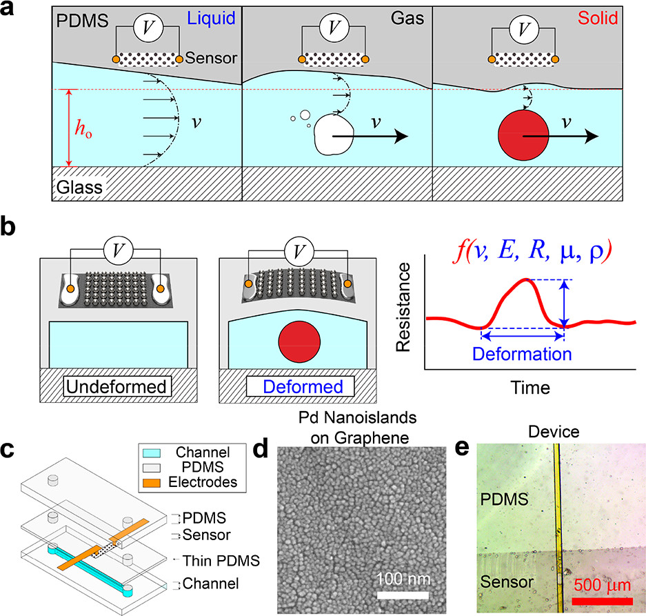
Figure 13: (a) Schematic of how a clear fluid (left), a bubbly fluid (center) and a particle-laden fluid (right) flow induces deformation of a soft channel wall made from PDMS. (b) The deformation is measured from a voltage change generated by a piezoresistive thin film embedded into the soft wall. The voltage depends on the elastic wall’s properties ($E$, $\nu$), fluid properties ($\mu=\eta_{0}$, $\rho$) and particle/bubble size ($R$). (c) Schematic of how the microchip with a deformable channel and embedded sensing electrodes is manufactured. (d) Scanning electron microscope (SEM) image of the piezoresistive thin films, which is made from “palladium nano-islands on graphene.” (e) Bright-field microscope image of a portion of the device. The fluid channel is visible as the vertical line in the center. Reprinted with permission from Dhong et al. 2018 Nano Lett. 18 5306–5311 [238]. Copyright (2018) American Chemical Society.

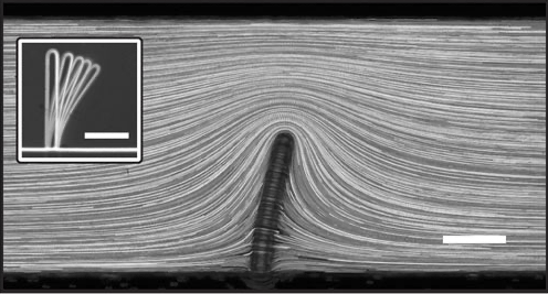
(a)

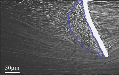
(b)

Figure 14: (a) Bending of a soft PDMS beam ($E=64\pm 22$ kPa) due to low-Reynolds-number Newtonian fluid (100% PEGDA-575) flow (left to right, visualized by pathlines). The beam height is $h_{b}=226$ $\mu$m in a channel that is $h_{0}=400$ $\mu$m tall. The flow is confined in the transverse direction across a depth of $d_{c}=45$ $\mu$m. The inset shows the deformation for flow rates $q=0,3,8,15$ and $30$ $\mu$L/min, while the main image is for $3$ $\mu$L/min. Scale bars represent $100$ $\mu$m. Reproduced from [245] with permission from Cambridge University Press © 2013. (b) Bending of a soft PDMS beam ($E=2\pm 0.3$ MPa) due to low-Reynolds-number non-Newtonian polymeric fluid (Flopaam 3630 mixed with deionized water at a concentration of 0.02% by weight) flow (left to right, visualized by streaklines) at finite Weissenberg number. Dimensions are similar to (a). Dark field imaging reveals flow fluctuations and vortex shedding in the circled region, despite the negligible flow inertia. Reproduced from [246] with permission from The Royal Society of Chemistry © 2020.

5.5 Rigid walls, soft obstacles

Viscous flow past a deformable (soft) beam is a classical problem in fluid–structure interactions (see, e.g., the numerous examples in [25]). In fact, a version of this problem (in which a channel flow is parallel to the beam) is a benchmark for numerical methods for fluid–structure interaction (the so-called Turek–Hron problem [247]). In a rigid channel, an anchored series of elastic fibers (“hairs”) can deform due to flow, thus increase the flow area much like a compliant wall (as in section 3). However, when the fibers are cantilevered at an angle towards the wall, they were shown to decrease the flow area, producing a “a rectification nonlinearity” [248], which can be harnessed for designing diodes and generating pumping in microfluidics.

In this context, Wexler et al. [245] performed experiments (figure 14(a)) and modeling of this problem, demonstrating that the tip deflection $u_{\mathrm{tip}}$ of the beam due to Newtonian fluid flow obeys

$$\eqalign{u_{\mathrm{tip}}\simeq\frac{6\eta_{0}(d_{c}+d)h_{0}^{4}q}{EId_{c}^{3}}\\ \quad\times\left\{\begin{array}[]{@{}l@{\quad}l}0.15(h_{b}/h_{0})^{5},&h_{b}\ll h_{0},\\ \frac{1}{2\pi}\log(1-h_{b}/h_{0})^{-1}-0.176,&h_{b}\to h_{0},\end{array}\right.}$$

where $I=dw^{3}/12$ is the moment of inertia of the beam, $h_{b}$ is the deformed length of the beam, $h_{0}$ is the height of the channel, $d_{c}$ is the transverse confinement dimension, and the beam has rectangular cross-section $d\times w$.

For the Newtonian case shown in figure 14(a), no instabilities or unsteady effects are observed. However, if the working fluid is a polymeric solution (with stress relaxation time $\lambda_{r}$, as in section 3.2.2), then purely elastic instabilities can occur even at vanishing Reynolds number (in the absence of inertia) [166, 167, 168]. The dimensionless number quantifying this non-Newtonian effect is the Weissenberg number [249]:

$$Wi=\frac{\mathrm{flow~{}elastic~{}forces}}{\mathrm{flow~{}viscous~{}forces}}\simeq\lambda_{r}\dot{\gamma}=\frac{\lambda_{r}q}{d_{c}^{2}(h_{0}-h_{b})}$$ (67)

for the flow in figure 14. Dey et al. [246, 250] demonstrated that at finite $Wi=\mathcal{O}(1)$, these viscoelastic fluid–structure interactions lead to instabilities, vortex shedding off the beam, and generally unsteady flows (figure 14(b)). The physical mechanism behind this sequence of events is distinctly different from vortex shedding past a beam due to inertia (finite Reynolds number) in Newtonian fluid flows. Understanding the physics of these viscoelastic microscale fluid–structure interactions past soft obstacles, and if and when they lead to predictable steady flows, is relevant for flow rate sensors and actuators for non-Newtonian fluids in microfluidics. As the problem is now unsteady and the flow is complex, a theoretical result such as (5.5) is not available. Nevertheless, the frequency and amplitude of the beam’s oscillations were measured as functions of $Wi$ for different types of polymeric liquids [246, 250].

6 Conclusions and outlook

From labs-on-a-chip that analyze biological fluid samples (such as blood and saliva) to miniaturized devices that mimic the behavior of organs, microfluidics requires the manipulation of not only Newtonian but also non-Newtonian (complex) fluids. Cheap and facile manufacturing of the flow conduits in these devices from soft polymeric materials, such as PDMS, leads to flow-induced deformation of the passages. On the one hand, this is a side effect to be analyzed and avoided. On the other hand, compliance opens up new avenues for flexible microdevices, pumping, valving, mixing and so on. At the intersection of non-Newtonian fluid mechanics and soft matter physics, flows of complex fluids through compliant conduits remains an active topic of research in this emerging field of soft hydraulics. Experiments have provided a number of observations, as well as new puzzles, that merit careful study. As theory catches up, predictive physical models are emerging to rationalize experiments. Much of the “conventional wisdom” on flows in compliant conduits has come from understanding the physics of Newtonian fluid flows. The focus has been on this case because it allows for significant progress in the mathematical analysis of challenging problems involving the coupled 3D equations of fluid mechanics and elasticity. Thus, non-Newtonian fluid flows through soft hydraulic conduits is a topic at the foreground of ongoing research, as summarized in this review.

From the practical point of view, this review surveyed the key physics from the recent literature, and provided a “recipe” for building predictive analytical models, as outlined in the stated scope (section 1.1). First, the relationship between volumetric flow rate and axial pressure gradient is needed for a given flow (section 3.4). This relationship is challenging (or impossible) to obtain in closed analytical form for most non-Newtonian fluids with shear-dependent viscosity. Notable exceptions are the power-law and Ellis models of the effective viscosity. Then, the channel height or tube radius in the pressure gradient–flow rate relation is to be replaced with an expression that accounts for the pressure-induced deformation of the height/radius of the conduit (section 3.5), suitably derived from the theory of elasticity. To solve the coupled problem, and obtain an analytical model, it is necessary to be able to “separate” (and integrate) the resulting ODE for the pressure (section 3.6). This manipulation is also not always possible analytically. However, at this point, even a straightforward numerical integration can be used to obtain the pressure distribution in the soft hydraulic conduit, from which all other quantities follow. It should be emphasized that these new theoretical developments require quantitative validation against novel, precise experiments and across a range of flow conditions (i.e., shear rates) for which the Carreau rheological model is best suited [251].

The discussion in this review focused mainly on non-Newtonian fluids with a shear-dependent viscosity at steady state. It is worth noting that there are few conclusive experimental or theoretical results on the flow rate–pressure drop characteristics of steady viscoelastic flows at the microscale (low Reynolds number), much less through non-uniform or deformable conduits (see, e.g., the discussions in [98, 99]). Notably, Boyko and Stone [252] recently showed how to use the reciprocal theorem for Stokes flow to calculate the leading-order non-Newtonian correction to the pressure drop–flow rate relation, using only the Newtonian base flow solution in a two-dimensional slowly-varying conduit of given shape. Indeed, the relevance of these non-Newtonian fluids flows to microfluidics is established [82]. However, the physical mechanism for why viscoelasticity (due to, e.g., just 0.01% of a high-molecular-weight polymer added to an aqueous solution) leads to anisotropic flow resistance remains to be understood theoretically [253]. Nevertheless, Groisman et al. [254] were able to exploit this viscoelastic fluid flow effect to design circuit elements, such as rectifiers and diodes, for fluidic control.

While certain open problems and suggested generalizations of the quoted results were noted along the way, it is now important to identify a number of fundamental topics that have not been addressed by research and experiments on soft hydraulics. Complex fluids (especially biological fluids) might exhibit wall-shear-stress dependent slip [255], for which some exact solutions generalizing those in section 3.4 are known [256]. (For Newtonian fluid flow in a compliant microchannel with a patterned bottom solid wall that engenders linear Navier slip, Karan et al. [257] recently developed a model along the lines of section 3.6.) Next, although the deformation of PDMS-based microfluidics channels is well described by the theory of linear elasticity, at large enough pressures, geometric nonlinearities (such as stretching) can arise [54, 115]. Buckling is also possible, which can be harnessed to design a “passive fuse” [258]. In these cases, the present state of the art, is to employ a deformation–pressure correlation for stretching of thin shells (e.g., [259, pp. 29–33]) for the deformation–pressure relationship (section 3.5). A more general approach is to derive such a relationship from nonlinear beam [207] and shell [260] theories, as commonly done in the literature on collapsible tubes, which undergo large elastic deformation [42, 40, 41].

Under large loads, PDMS can also exhibit material nonlinearity (hyperelastic response) [261], which can also be handled within the framework reviewed herein [116]. Viscoelastic behavior of the working fluid was discussed in this review. However, the compliant conduit’s walls can themselves exhibit viscoelastic response [262] (although typical PDMS mixtures have a weak viscoelastic response [263]). Furthermore, poroelasticity of the conduit might also be important if dealing with hydrogel materials [262], within which biomimetic “hierarchically branched vascular networks” of microchannels with porous walls resemble tissues [264]. Auton and MacMinn [265, 266] considered the flow-induced deformation a of poroelastic cylinder saturated with a Newtonian fluid. It would be of interest to generalize the results reviewed herein (focused on elasticity of the conduit walls only) to such hyper-, visco-, and poroelastic response of the walls due to the flow of a non-Newtonian fluid within [267].

In conclusion, it is fitting to recall the last sentence of the 2004 review by Stone et al. [1]: “These [microfluidic] systems should provide challenges in fluid dynamics, transport, and engineering design for generations of readers.” Indeed, as the latter review matures to two decades, the next generation of readers has emerged. Undoubtedly, the challenges of non-Newtonian fluid dynamics, elastic deformation of soft materials, and engineering design at the microscale will continue to puzzle and delight them.

Data availability statement

The data that support the findings of this study are available upon reasonable request from the authors.

ORCID iDs

Ivan C. Christov  https://orcid.org/0000-0001-8531-0531

References

- [1] Stone H A, Stroock A D and Ajdari A 2004 Annu. Rev. Fluid Mech. 36 381–411
- [2] Squires T M and Quake S R 2005 Rev. Mod. Phys. 77 977–1026
- [3] Nguyen N T and Wereley S T 2006 Fundamentals and Applications of Microfluidics 2nd ed Integrated Microsystems Series (Norwood, MA: Artech House)
- [4] Kim Y, Messner W C and LeDuc P R 2012 Disruptive Sci. Tech. 1 41–53
- [5] El-Ali J, Sorger P K and Jensen K F 2006 Nature 442 403–411
- [6] Prakash M and Gershenfeld N 2007 Science 315 832–835
- [7] Katsikis G, Cybulski J S and Prakash M 2015 Nat. Phys. 11 588–596
- [8] Whitesides G M 2006 Nature 442 368–373
- [9] Grand View Research 2021 Microfluidics market size, share & trends analysis report Tech. Rep. GVR-1-68038-056-9 URL https://www.grandviewresearch.com/industry-analysis/microfluidics-market
- [10] McDonald J C and Whitesides G M 2002 Acc. Chem. Res. 35 491–499
- [11] Lötters J C, Olthuis W, Veltink P H and Bergveld P 1997 J. Micromech. Microeng. 7 145–147
- [12] Johnston I D, McCluskey D K, Tan C K L and Tracey M C 2014 J. Micromech. Microeng. 24 35017
- [13] Allen M 2017 Microfluidic chip can detect HIV and MRSA Physics World URL https://physicsworld.com/a/microfluidic-chip-can-detect-hiv-and-mrsa/
- [14] Yeh E C, Fu C C, Hu L, Thakur R, Feng J and Lee L P 2017 Sci. Adv. 3 e1501645
- [15] Xia Y and Whitesides G M 1998 Annu. Rev. Mater. Sci. 28 153–184
- [16] Liu M, Sun J, Sun Y, Bock C and Chen Q 2009 J. Micromech. Microeng. 19 035028
- [17] Gervais T, El-Ali J, Günther A and Jensen K F 2006 Lab Chip 6 500–507
- [18] Yalikun Y, Ota N, Guo B, Tang T, Zhou Y, Lei C, Kobayashi H, Hosokawa Y, Li M, Enrique Muñoz H, Di Carlo D, Goda K and Tanaka Y 2020 Cytometry Part A 97 909–920
- [19] Delamarche E, Schmid H, Michel B and Biebuyck H 1997 Adv. Mat. 9 741–746
- [20] Hui C Y, Jagota A, Lin Y Y and Kramer E J 2002 Langmuir 18 1394–1407
- [21] Xu S, Zhang Y, Jia L, Mathewson K E, Jang K I, Kim J, Fu H, Huang X, Chava P, Wang R, Bhole S, Wang L, Na Y J, Guan Y, Flavin M, Han Z, Huang Y and Rogers J A 2014 Science 344 70–74
- [22] Yeo J C, Kenrya and Lim C T 2016 Lab Chip 16 4082–4090
- [23] Huh D, Matthews B D, Mammoto A, Montoya-Zavala M, Hsin H Y and Ingber D E 2010 Science 328 1662–1668
- [24] Lind J U, Busbee T A, Valentine A D, Pasqualini F S, Yuan H, Yadid M, Park S J, Kotikian A, Nesmith A P, Campbell P H, Vlassak J J, Lewis J A and Parker K K 2017 Nat. Mat. 16 303–308
- [25] Duprat C and Stone H A 2014 Fluid-Structure Interactions in Low-Reynolds-Number Flows (Cambridge, UK: Royal Society of Chemistry)
- [26] Païdoussis M P 2014 Fluid-Structure Interactions: Slender Structures and Axial Flow 2nd ed (San Diego, CA: Academic Press)
- [27] Gohar R 2001 Elastohydrodynamics 2nd ed (London: Imperial College Press)
- [28] Fung Y C 1997 Biomechanics: Circulation 2nd ed (New York: Springer)
- [29] Chakraborty S (ed) 2010 Microfluidics and Microfabrication (New York: Springer Science+Business Media)
- [30] Chakraborty S (ed) 2013 Microfluidics and Microscale Transport Processes IIT Kharagpur Research Monograph Series (Boca Raton, FL: CRC Press)
- [31] Das T and Chakraborty S 2010 Bio-microfluidics: Overview Microfluidics and Microfabrication ed Chakraborty S (New York: Springer Science+Business Media) chap 4, pp 131–179
- [32] Ho C M and Tai Y C 1998 Annu. Rev. Fluid Mech. 30 579–612
- [33] Gad-el Hak M 1999 ASME J. Fluids Eng. 121 5–33
- [34] Stone H A 2007 Introduction to fluid dynamics for microfluidic flows CMOS Biotechnology Series on Integrated Circuits and Systems ed Lee H, Westervelt R M and Ham D (New York, NY: Springer Science+Business Media, LLC) pp 5–30
- [35] Abgrall P and Gué A M 2007 J. Micromech. Microeng. 17 R15
- [36] Stoecklein D and Di Carlo D 2019 Anal. Chem. 91 296–314
- [37] Xia H M, Wu J W, Zheng J J, Zhang J and Wang Z P 2021 Lab Chip 21 1241–1268
- [38] Wang Y, Pilkington G A, Dhong C and Frechette J 2017 Curr. Opin. Colloid Interface Sci. 27 43–49
- [39] Wang Y, Tan M R and Frechette J 2017 Soft Matter 13 6718–6729
- [40] Grotberg J B and Jensen O E 2004 Annu. Rev. Fluid Mech. 36 121–147
- [41] Heil M and Hazel A L 2011 Annu. Rev. Fluid Mech. 43 141–162
- [42] Shapiro A H 1977 ASME J. Biomech. Eng. 99 126–147
- [43] Pedley T J 1980 The Fluid Mechanics of Large Blood Vessels (Cambridge: Cambridge University Press)
- [44] Lauga E and Powers T R 2009 Rep. Prog. Phys. 72 096601
- [45] Fallahi H, Zhang J, Phan H P and Nguyen N T 2019 Micromachines 10 830
- [46] Raj M K and Chakraborty S 2020 J. Appl. Polym. Sci. 137 48958
- [47] Karan P, Chakraborty J and Chakraborty S 2018 J. Indian Inst. Sci. 98 159–183
- [48] Cheung P, Toda-Peters K and Shen A Q 2012 Biomicrofluidics 6 026501
- [49] Bruus H 2008 Theoretical Microfluidics (Oxford: Oxford University Press)
- [50] Kirby B J 2010 Micro- and Nanoscale Fluid Mechanics: Transport in Microfluidic Devices (New York: Cambridge University Press)
- [51] Karniadakis G, Beskok A and Aluru N 2005 Microflows and Nanoflows: Fundamentals and Simulation (Interdisciplinary Applied Mathematics no 29) (New York, NY: Springer Science+Business Media)
- [52] Tabeling P 2005 Introduction to Microfluidics (Oxford, UK: Oxford University Press)
- [53] Anand V, Rathinaraj J D J and Christov I C 2019 J. Non-Newtonian Fluid Mech. 264 62–72
- [54] Raj A and Sen A K 2016 Microfluid Nanofluid 20 31
- [55] Raj M K, Chakraborty J, DasGupta S and Chakraborty S 2018 Biomicrofluidics 12 034116
- [56] Del Giudice F, Greco F, Netti P A and Maffettone P L 2016 Biomicrofluidics 10 043501
- [57] Nahar S, Dubey B N and Windhab E J 2019 Phys. Fluids 31 101905
- [58] Koo J and Kleinstreuer C 2003 J. Micromech. Microeng. 13 568–579
- [59] Oh K W, Lee K, Ahn B and Furlani E P 2012 Lab Chip 12 515–545
- [60] Lugt P M and Morales-Espejel G E 2011 Tribol. Trans. 54 470–496
- [61] Carvalho M S and Scriven L E 1997 J. Fluid Mech. 339 143–172
- [62] Yin X and Kumar S 2005 Phys. Fluids 17 063101
- [63] Purcell E M and Morin D J 2013 Electricity and Magnetism 3rd ed Electricity and Magnetism (New York, NY: Cambridge University Press)
- [64] Wang Y, Bedekar A S, Krishnamoorthy S, Sundaram S and Singhal A K 2008 Model Order Reduction (MOR) Encyclopedia of Microfluidics and Nanofluidics ed Li D (Boston, MA: Springer) pp 1382–1391
- [65] Sutera S P and Skalak R 1993 Annu. Rev. Fluid Mech. 25 1–19
- [66] Happel J R and Brenner H 1983 Low Reynolds Number Hydrodynamics with Special Applications to Particulate Media 2nd ed (The Hague: Martinus Nijhoff Publishers)
- [67] Lauga E, Stroock A D and Stone H A 2004 Phys. Fluids 16 3051–3062
- [68] White F M 2006 Viscous Fluid Flow 3rd ed (New York, NY: McGraw-Hill Higher Education)
- [69] Mortensen N A, Okkels F and Bruus H 2005 Phys. Rev. E 71 057301
- [70] Case D J, Liu Y, Kiss I Z, Angilella J R and Motter A E 2019 Nature 574 647–652
- [71] Ajdari A 2004 C. R. Phys. 5 539–546
- [72] Hardy B S, Uechi K, Zhen J and Kavehpour H P 2009 Lab Chip 9 935–938
- [73] Leslie D C, Easley C J, Seker E, Karlinsey J M, Utz M, Begley M R and Landers J P 2009 Nat. Phys. 5 231–235
- [74] Begley M R, Utz M, Leslie D C, Haj-Hariri H, Landers J and Bart-Smith H 2009 Appl. Phys. Lett. 95 203501
- [75] Seker E, Leslie D C, Haj-Hariri H, Landers J P, Utz M and Begley M R 2009 Lab Chip 9 2691–2697
- [76] Zengerle R and Richter M 1994 J. Micromech. Microeng. 4 192–204
- [77] Bird R B, Armstrong R C and Hassager O 1987 Dynamics of Polymeric Liquids 2nd ed vol 1 (New York: John Wiley)
- [78] Larson R G 1998 The Structure and Rheology of Complex Fluids Topics in Chemical Engineering (Oxford, UK: Oxford University Press)
- [79] Chhabra R P and Richardson J F 2008 Non-Newtonian Fluid Behaviour 2nd ed (Oxford: Butterworth-Heinemann)
- [80] Owens R G and Phillips T N 2002 Computational Rheology (London: Imperial College Press)
- [81] Nijenhuis K, McKinley G H, Spiegelberg S, Barnes H A, Aksel N, Heymann L and Odell J A 2007 Non-Newtonian flows Springer Handbook of Experimental Fluid Mechanics ed Tropea C, Yarin A L and Foss J F (Berlin/Heidelberg: Springer-Verlag) chap 9, pp 619–743
- [82] Anna S L 2008 Non-Newtonian fluids in microfluidics Encyclopedia of Microfluidics and Nanofluidics ed Li D (Boston, MA: Springer) pp 1480–1488
- [83] Chakraborty S 2008 Non-Newtonian fluids in microchannel Encyclopedia of Microfluidics and Nanofluidics ed Li D (Boston, MA: Springer) pp 1471–1480
- [84] Boger D V 1977 Nature 265 126–128
- [85] Pritchard P J 2011 Fox & McDonald’s Introduction to Fluid Mechanics 8th ed (Hoboken, NJ: John Wiley & Sons)
- [86] Leal L G 2007 Advanced Transport Phenomena: Fluid Mechanics and Convective Transport Processes (Cambridge Series in Chemical Engineering vol 7) (New York, NY: Cambridge University Press)
- [87] Lee L J 2006 BioMEMS Encyclopedia of Chemical Processing vol 1 ed Lee S (New York: Taylor & Francis) pp 161–169
- [88] Basaran O A, Gao H and Bhat P P 2013 Annu. Rev. Fluid Mech. 45 85–113
- [89] Das S and Chakraborty S 2006 Anal. Chim. Acta 559 15–24
- [90] Steller R T 2001 Polym. Eng. Sci. 41 1859–1870
- [91] Ciriello V, Lenci A, Longo S and Di Federico V 2021 Adv. Water. Res. 152 103914
- [92] Balmforth N J, Frigaard I A and Ovarlez G 2014 Annu. Rev. Fluid Mech. 46 121–146
- [93] Fung Y C 1993 Biomechanics: Mechanical Properties of Living Tissues (New York, NY: Springer)
- [94] Ayyaswamy P S 2016 Introduction to biofluid mechanics Fluid Mechanics ed Kundu P K, Cohen I M and Dowling D R (San Diego, CA: Academic Press) chap 16, pp e1–e73 6th ed
- [95] Chakraborty S 2005 Lab Chip 5 421–430
- [96] Christov I C and Christov C I 2016 Mech. Res. Commun. 72 59–63
- [97] Oliveira M S N, Alves M A and Pinho F T 2011 Microfluidic flows of viscoelastic fluids Transport and Mixing in Laminar Flows: From Microfluidics to Oceanic Currents ed Grigoriev R (Weinheim, Germany: Wiley‐VCH Verlag) chap 6, pp 131–174
- [98] Rothstein J P and McKinley G H 2001 J. Non-Newtonian Fluid Mech. 98 33–63
- [99] Koppol A P, Sureshkumar R, Abedijaberi A and Khomami B 2009 J. Fluid Mech. 631 231—253
- [100] Ramos-Arzola L and Bautista O 2021 J. Non-Newtonian Fluid Mech. 296 104634
- [101] Christov I C, Cognet V, Shidhore T C and Stone H A 2018 J. Fluid Mech. 841 267–286
- [102] Reynolds O 1886 Phil. Trans. R. Soc. Lond. 177 157–234
- [103] Reynolds O 1883 Phil. Trans. R. Soc. Lond. A 174 935–982
- [104] Jackson D and Launder B 2007 Annu. Rev. Fluid Mech. 39 19–35
- [105] Stone H A 2017 Fundamentals of fluid dynamics with an introduction to the importance of interfaces Soft Interfaces (Lecture Notes of the Les Houches Summer School vol 98) ed Bocquet L, Quéré D, Witten T A and Cugliandolo L F (New York, NY: Oxford University Press) chap 1, pp 3–76
- [106] Boyko E, Bercovici M and Gat A D 2017 Phys. Rev. Fluids 2 073301
- [107] Anand V and Christov I C 2021 Z. Angew. Math. Mech. (ZAMM) 101 e201900309
- [108] Van Dyke M 1987 Adv. Appl. Mech. 25 1–45
- [109] Wang X and Christov I C 2019 Proc. R. Soc. A 475 20190513
- [110] Elbaz S B and Gat A D 2014 J. Fluid Mech. 758 221–237
- [111] Rubinow S I and Keller J B 1972 J. Theor. Biol. 34 299–313
- [112] Iliev O, Mikelić A and Popov P 2008 Multiscale Model. Simul. 7 93–123
- [113] Rosti M E, Pramanik S, Brandt L and Mitra D 2020 Soft Matter 16 939–944
- [114] Unger M A, Chou H P, Thorsen T, Scherer A and Quake S R 2000 Science 288 113–116
- [115] Shidhore T C and Christov I C 2018 J. Phys.: Condens. Matter 30 054002
- [116] Anand V and Christov I C 2019 On the deformation of a hyperelastic tube due to steady viscous flow within Dynamical Processes in Generalized Continua and Structures (Advanced Structured Materials vol 103) ed Altenbach H, Belyaev A, Eremeyev V, Krivtsov A and Porubov A (Cham, Switzerland: Springer Nature) pp 17–35
- [117] Anand V, Muchandimath S C and Christov I C 2020 ASME J. Appl. Mech. 87 051012
- [118] Raj M K, DasGupta S and Chakraborty S 2017 Microfluid. Nanofluid. 21 70
- [119] Hunter L, Gala de Pablo J, Stammers A C, Thomson N H, Evans S D and Shim J u 2020 SN Appl. Sci. 2 1501
- [120] Howell P, Kozyreff G and Ockendon J 2009 Applied Solid Mechanics (Cambridge, UK: Cambridge University Press)
- [121] Skotheim J M and Mahadevan L 2004 Phys. Rev. Lett. 92 245509
- [122] Skotheim J M and Mahadevan L 2005 Phys. Fluids 17 092101
- [123] Chakraborty J and Chakraborty S 2011 Phys. Fluids 23 082004
- [124] Kiran Raj M, Dasgupta S and Chakraborty S 2019 Biomicrofluidics 13 14103
- [125] Ramachandran V and Majidi C 2018 ASME J. Appl. Mech. 85 101004
- [126] Wang X and Christov I C 2021 Phys. Fluids 33 102004
- [127] Dillard D A, Mukherjee B, Karnal P, Batra R C and Frechette J 2018 Soft Matter 14 3669–3683
- [128] Chandler T G J and Vella D 2020 Proc. R. Soc. A 476 20200551
- [129] Salem L, Gamus B, Or Y and Gat A D 2020 Soft Robotics 7 76–84
- [130] Lee G, Luner A, Marzuola J and Harris D M 2021 Microfluid. Nanofluid. 25 34
- [131] Sochi T 2015 Rheol. Acta 54 745–756
- [132] Pritchard D and Corson L T 2015 Rheol. Acta 54 657–659
- [133] Boyko E and Stone H A 2021 J. Fluid Mech. 923 R5
- [134] Mehboudi A and Yeom J 2019 Microfluid. Nanofluid. 23 66
- [135] Christopher G F, Yoo J M, Dagalakis N, Hudson S D and Migler K B 2010 Lab Chip 10 2749–2757
- [136] Baum M 2010 Micro rheometer is latest lab on a chip device NIST News URL https://www.nist.gov/news-events/news/2010/08/micro-rheometer-latest-lab-chip-device
- [137] Pipe C J and McKinley G H 2009 Mech. Res. Commun. 36 110–120
- [138] Gupta S, Wang W S and Vanapalli S A 2016 Biomicrofluidics 10 043402
- [139] Del Giudice F, D’Avino G, Greco F, De Santo I, Netti P A and Maffettone P L 2015 Lab Chip 15 783–792
- [140] Srivastava N and Burns M A 2006 Anal. Chem. 78 1690–1696
- [141] Galindo-Rosales F J, Alves M A and Oliveira M S N 2013 Microfluid. Nanofluid. 14 1–19
- [142] Hudson S D, Sarangapani P, Pathak J A and Migler K B 2015 J. Pharm. Sci. 104 678–685
- [143] Vishwanathan G and Juarez G 2020 Microfluid. Nanofluid. 24 69
- [144] Riley N 2001 Annu. Rev. Fluid Mech. 33 43–65
- [145] Sadhal S S 2012 Lab Chip 12 2292–2300
- [146] Vishwanathan G and Juarez G 2019 Phys. Fluids 31 041701
- [147] Vishwanathan G and Juarez G 2019 J. Non-Newtonian Fluid Mech. 271 104143
- [148] Muzychka Y S and Edge J 2008 ASME J. Fluids Eng. 130 111201
- [149] Sharp K V, Adrian R J, Santiago J G and Molho J I 2001 Liquid flows in microchannels The MEMS Handbook ed Gad-el Hak M (Boca Raton, FL: CRC Press) chap 6
- [150] Yang X, Weldetsadik N T, Hayat Z, Fu T, Jiang S, Zhu C and Ma Y 2019 Microfluid. Nanofluid. 23 75
- [151] Kang K, Lee L J and Koelling K W 2005 Exp. Fluids 38 222–232
- [152] Pipe C J, Majmudar T S and McKinley G H 2008 Rheol. Acta 47 621–642
- [153] Shiba K, Li G, Virot E, Yoshikawa G and Weitz D A 2021 Lab Chip 21 2805–2811
- [154] Stroock A D, Dertinger S K W, Ajdari A, Mezić I, Stone H A and Whitesides F M 2002 Science 295 647–651
- [155] Verma M K S and Kumaran V 2013 J. Fluid Mech. 727 407–455
- [156] Srinivas S S and Kumaran V 2017 J. Fluid Mech. 812 1076–1118
- [157] Chandra B, Shankar V and Das D 2019 Phys. Fluids 31 114103
- [158] Reyes D R, Iossifidis D, Auroux P A and Manz A 2002 Anal. Chem. 74 2623–2636
- [159] Auroux P A, Iossifidis D, Reyes D R and Manz A 2002 Anal. Chem. 74 2637–2652
- [160] Yetisen A K, Akram M S and Lowe C R 2013 Lab Chip 13 2210–2251
- [161] Sackmann E K, Fulton A L and Beebe D J 2014 Nature 507 181–189
- [162] Yager P, Edwards T, Fu E, Helton K, Nelson K, Tam M R and Weigl B H 2006 Nature 442 412–418
- [163] Karnik R 2013 Microfluidic mixing Encyclopedia of Microfluidics and Nanofluidics ed Li D (Boston, MA: Springer) pp 1–13
- [164] National Committee for Fluid Mechanics Films 1967 Low Reynolds number flow Education Development Center, Inc. URL http://web.mit.edu/hml/ncfmf.html
- [165] Ottino J M and Wiggins S 2004 Phil. Trans. R. Soc. A 362 923–935
- [166] Larson R G 1992 Rheol. Acta 31 213–263
- [167] Shaqfeh E S G 1996 Annu. Rev. Fluid Mech. 28 129–185
- [168] Steinberg V 2021 Annu. Rev. Fluid Mech. 53 27–58
- [169] Li X B, Li F C, Cai W H, Zhang H N and Yang J C 2012 Exp. Thermal Fluid Sci. 39 1–16
- [170] Galindo-Rosales F J, Campo-Deaño L, Sousa P C, Ribeiro V M, Oliveira M S N, Alves M A and Pinho F T 2014 Exp. Thermal Fluid Sci. 59 128–139
- [171] Aref H 1984 J. Fluid Mech. 143 1–21
- [172] Ottino J M 1989 The Kinematics of Mixing: Stretching, Chaos, and Transport (Cambridge Texts in Applied Mathematics vol 3) (Cambridge, UK: Cambridge University Press)
- [173] Thakur R K, Vial C, Nigam K D P, Nauman E B and Djelveh G 2003 Chem. Eng. Res. Des. 81 787–826
- [174] Ghanem A, Lemenand T, Valle D D and Peerhossaini H 2014 Chem. Eng. Res. Des. 92 205–228
- [175] Krindel P and Silberberg A 1979 J. Colloid Interface Sci. 71 39–50
- [176] Verma M K S and Kumaran V 2013 J. Fluid Mech. 705 322–347
- [177] Kumaran V and Bandaru P 2016 Chem. Eng. Sci. 149 156–168
- [178] Eckhardt B, Schneider T M, Hof B and Westerweel J 2007 Annu. Rev. Fluid Mech. 39 447–468
- [179] Sharp K V and Adrian R J 2004 Experiments in Fluids 36 741–747
- [180] Lee C Y, Chang C L, Wang Y N and Fu L M 2011 Int. J. Mol. Sci. 12 3263–3287
- [181] Friend J and Yeo L Y 2011 Rev. Mod. Phys. 83 647–704
- [182] Rallabandi B, Wang C and Hilgenfeldt S 2017 Phys. Rev. Fluids 2 064501
- [183] Chokshi P and Kumaran V 2007 Phys. Fluids 19 104103
- [184] Chokshi P, Bhade P and Kumaran V 2015 Phys. Rev. E 91 023007
- [185] Toner M 2018 “Extreme” microfluidics: Large-volumes and complex fluids Nobel Symposium 162 - Microfluidics, Nobel162/2017/09 Nobel Foundation URL https://arxiv.org/abs/1802.05600
- [186] Bhagat A A S, Kuntaegowdanahalli S S and Papautsky I 2008 Lab Chip 8 1906–1914
- [187] Di Carlo D 2009 Lab Chip 9 3038–3046
- [188] Di Carlo D, Irimia D, Tompkins R G and Toner M 2007 Proc. Natl Acad. Sci. USA 104 18892–18897
- [189] Lim E J, Ober T J, Edd J F, Desai S P, Neal D, Bong K W, Doyle P S, McKinley G H and Toner M 2014 Nat. Commun. 5 4120
- [190] Riley J J, Gad-el-Hak M and Metcalfe R W 1988 Annu. Rev. Fluid Mech. 20 393–420
- [191] Gad-el Hak M 1996 Appl. Mech. Rev. 49 S147–S157
- [192] Gad-el Hak M 2002 Prog. Aerospace Sci. 38 77–99
- [193] Kramer M O 1961 J. Am. Soc. Naval Eng. 73 103–108
- [194] Benjamin T B 1960 J. Fluid Mech. 9 513–532
- [195] Neelamegam R and Shankar V 2015 Phys. Fluids 27 024102
- [196] Patne R and Shankar V 2019 J. Fluid Mech. 860 837–885
- [197] Tanmay V S, Patne R and Shankar V 2018 Phys. Fluids 30 074103
- [198] Kumaran V 2021 J. Fluid Mech. 924 P1
- [199] Karan P, Das S S, Mukherjee R, Chakraborty J and Chakraborty S 2020 Soft Matter 16 5777–5786
- [200] Dendukuri D, Gu S S, Pregibon D C, Hatton T A and Doyle P S 2007 Lab Chip 7 818–828
- [201] Mukherjee U, Chakraborty J and Chakraborty S 2013 Soft Matter 9 1562–1569
- [202] Martínez-Calvo A, Sevilla A, Peng G G and Stone H A 2020 J. Fluid Mech. 885 A25
- [203] Elbaz S B, Jacob H and Gat A D 2018 J. Fluid Mech. 846 460–481
- [204] Anand V and Christov I C 2020 Phys. Fluids 32 112014
- [205] Holmes M H 2013 Introduction to Perturbation Methods 2nd ed (Texts in Applied Mathematics vol 20) (New York, NY: Springer)
- [206] Barenblatt G I 1996 Similarity, Self-Similarity, and Intermediate Asymptotics (Cambridge Texts in Applied Mathematics vol 14) (New York, NY: Cambridge University Press)
- [207] Inamdar T C, Wang X and Christov I C 2020 Phys. Rev. Fluids 5 064101
- [208] Garg V, Kamat P M, Anthony C R, Thete S S and Basaran O A 2017 J. Fluid Mech. 826 455–483
- [209] Vurgaft A, Elbaz S B and Gat A D 2019 J. Fluid Mech. 881 1048–1072
- [210] Peretz O, Mishra A K, Shepherd R F and Gat A D 2020 Proc. Natl Acad. Sci. USA 117 5217–5221
- [211] Elbaz S B and Gat A D 2016 J. Fluid Mech. 806 580–602
- [212] Polygerinos P, Correll N, Morin S A, Mosadegh B, Onal C D, Petersen K, Cianchetti M, Tolley M T and Shepherd R F 2017 Adv. Eng. Mater. 19 1700016
- [213] Chiapponi L, Ciriello V, Longo S and Di Federico V 2019 Water Res. Res. 55 10144–10158
- [214] Barbati A C, Desroches J, Robisson A and McKinley G H 2016 Annu. Rev. Chem. Biomol. Eng. 7 415–453
- [215] Dana A, Zheng Z, Peng G G, Stone H A, Huppert H E and Ramon G Z 2018 J. Fluid Mech. 836 828–849
- [216] Probstein R F 1994 Physicochemical Hydrodynamics: An Introduction 2nd ed (New York, NY: John Wiley & Sons)
- [217] Li D 2004 Electrokinetics in Microfluidics (Interface Science and Technology vol 2) (San Diego, CA: Elsevier)
- [218] Chakraborty D and Chakraborty S 2010 Microfluidic transport and micro-scale flow physics: An overview Microfluidics and Microfabrication ed Chakraborty S (New York: Springer Science+Business Media) chap 1, pp 1–85
- [219] Ghosal S 2010 Mathematical modeling of electrokinetic effects in micro and nano fluidics Microfluidics and Microfabrication ed Chakraborty S (New York: Springer Science+Business Media) chap 2, pp 87–112
- [220] Alizadeh A, Hsu W L, Wang M and Daiguji H 2021 Electrophoresis 42 834–868
- [221] Chakraborty J and Chakraborty S 2010 Phys. Fluids 22 122002
- [222] Steinberger A, Cottin-Bizonne C, Kleimann P and Charlaix E 2008 Phys. Rev. Lett. 100 134501
- [223] Das S, Chakraborty J and Chakraborty S 2013 Electrokinetics in narrow confinements Microfluidics and Microscale Transport Processes IIT Kharagpur Research Monograph Series ed Chakraborty S (Boca Raton, FL: CRC Press) chap 2, pp 49–110
- [224] Rubin S, Tulchinsky A, Gat A D and Bercovici M 2017 J. Fluid Mech. 812 841–865
- [225] Boyko E, Eshel R, Gommed K, Gat A D and Bercovici M 2019 J. Fluid Mech. 862 732–752
- [226] de Rutte J M, Janssen K G H, Tas N R, Eijkel J C T and Pennathur S 2016 Microfluid. Nanofluid. 20 150
- [227] Boyko E, Eshel R, Gat A D and Bercovici M 2020 Phys. Rev. Lett. 124 024501
- [228] Boyko E, Ilssar D, Bercovici M and Gat A D 2020 Phys. Rev. Fluids 5 104201
- [229] Hosoi A E and Mahadevan L 2004 Phys. Rev. Lett. 93 137802
- [230] Zhao C and Yang C 2013 Adv. Colloid Interface Sci. 201-202 94–108
- [231] Zhao C, Zholkovskij E, Masliyah J H and Yang C 2008 J. Colloid Interface Sci. 326 503–510
- [232] Zhao C and Yang C 2011 J. Non-Newtonian Fluid Mech. 166 1076–1079
- [233] Zimmerman W B, Rees J M and Craven T J 2006 Microfluid. Nanofluid. 2 481–492
- [234] Chakraborty S 2019 Electrophoresis 40 180–189
- [235] Karan P, Chakraborty J and Chakraborty S 2020 Phys. Fluids 32 022002
- [236] Karan P, Chakraborty J and Chakraborty S 2021 J. Fluid Mech. 923 A32
- [237] Naik K G, Chakraborty S and Chakraborty J 2017 Soft Matter 13 6422–6429
- [238] Dhong C, Edmunds S J, Ramírez J, Kayser L V, Chen F, Jokerst J V and Lipomi D J 2018 Nano Lett. 18 5306–5311
- [239] Ozsun O, Yakhot V and Ekinci K L 2013 J. Fluid Mech. 734 R1
- [240] Niu P, Nablo B J, Bhadriraju K and Reyes D R 2017 Anal. Chem. 89 11372–11377
- [241] Chen X, Falzon L, Zhang J, Zhang X, Wang R Q and Du K 2019 Nanotechnology 31 05LT01
- [242] Essink M H, Pandey A, Karpitschka S, Venner C H and Snoeijer J H 2021 J. Fluid Mech. 915 A49
- [243] D’Avino G, Greco F and Maffettone P L 2017 Annu. Rev. Fluid Mech. 49 341–360
- [244] Zhou J and Papautsky I 2020 Microsyst. Nanoeng. 6 113
- [245] Wexler J S, Trinh P H, Berthet H, Quennouz N, du Roure O, Huppert H E, Lindner A and Stone H A 2013 J. Fluid Mech. 720 517–544
- [246] Dey A A, Modarres-Sadeghi Y, Lindner A and Rothstein J P 2020 Soft Matter 16 1227–1235
- [247] Turek S and Hron J 2006 Proposal for numerical benchmarking of fluid-structure interaction between an elastic object and laminar incompressible flow Fluid-Structure Interaction (Lecture Notes in Computational Science and Engineering vol 53) ed Bungartz H J and Schäfer M (Berlin/Heidelberg: Springer) pp 371–385
- [248] Alvarado J, Comtet J, de Langre E and Hosoi A E 2017 Nat. Phys. 13 1014–1019
- [249] Poole R J 2012 Rheology Bulletin 53(2) 32–39 URL http://pcwww.liv.ac.uk/~robpoole/PAPERS/POOLE_45.pdf
- [250] Dey A A, Modarres-Sadeghi Y and Rothstein J P 2020 J. Non-Newtonian Fluid Mech. 286 104433
- [251] Moukhtari F E and Lecampion B 2018 J. Fluid Mech. 838 573–605
- [252] Boyko E and Stone H A 2021 Phys. Rev. Fluids 6 L081301
- [253] Groisman A and Quake S R 2004 Phys. Rev. Lett. 92 094501
- [254] Groisman A, Enzelberger M and Quake S R 2003 Science 300 955–958
- [255] Granick S, Zhu Y and Lee H 2003 Nature Materials 2 221–227
- [256] Ferrás L L, Nóbrega J M and Pinho F T 2012 J. Non-Newtonian Fluid Mech. 175-176 76–88
- [257] Karan P, Chakraborty J, Chakraborty S, Wereley S T and Christov I C 2021 Phys. Rev. E 104 015108
- [258] Gomez M, Moulton D E and Vella D 2017 Phys. Rev. Lett. 119 144502
- [259] Schomburg W K 2011 Introduction to Microsystem Design (Berlin/Heidelberg: Springer-Verlag)
- [260] Whittaker R J, Heil M, Jensen O E and Waters S L 2010 Q. J. Mech. Appl. Math. 63 465–496
- [261] Nunes L C S 2011 Mat. Sci. Eng. A 528 1799–1804
- [262] Hu Y and Suo Z 2012 Acta Mech. Solida Sin. 25 441–458
- [263] Lin I K, Ou K S, Liao Y M, Liu Y, Chen K S and Zhang X 2009 J. Microelectromech. Syst. 18 1087–1099
- [264] Huang G Y, Zhou L H, Zhang Q C, Chen Y M, Sun W, Xu F and Lu T J 2011 Biofabrication 3 012001
- [265] Auton L C and MacMinn C W 2017 Proc. R. Soc. A 473 20160753
- [266] Auton L C and MacMinn C W 2018 Proc. R. Soc. A 474 20180284
- [267] Ambartsumyan I, Ervin V J, Nguyen T and Yotov I 2019 ESAIM: M2AN 53 1915–1955