Iterative Methods for Private Synthetic Data:
Unifying Framework and New Methods

Abstract

We study private synthetic data generation for query release, where the goal is to construct a sanitized version of a sensitive dataset, subject to differential privacy, that approximately preserves the answers to a large collection of statistical queries. We first present an algorithmic framework that unifies a long line of iterative algorithms in the literature. Under this framework, we propose two new methods. The first method, private entropy projection (PEP), can be viewed as an advanced variant of MWEM that adaptively reuses past query measurements to boost accuracy. Our second method, generative networks with the exponential mechanism (GEM), circumvents computational bottlenecks in algorithms such as MWEM and PEP by optimizing over generative models parameterized by neural networks, which capture a rich family of distributions while enabling fast gradient-based optimization. We demonstrate that PEP and GEM empirically outperform existing algorithms. Furthermore, we show that GEM nicely incorporates prior information from public data while overcoming limitations of PMW^Pub, the existing state-of-the-art method that also leverages public data.

1 Introduction

As the collection and analyses of sensitive data become more prevalent, there is an increasing need to protect individuals’ private information. Differential privacy [DworkMNS06] is a rigorous and meaningful criterion for privacy preservation that enables quantifiable trade-offs between privacy and accuracy. In recent years, there has been a wave of practical deployments of differential privacy across organizations such as Google, Apple, and most notably, the U.S. Census Bureau [Abowd18].

In this paper, we study the problem of differentially private query release: given a large collection of statistical queries, the goal is to release approximate answers subject to the constraint of differential privacy. Query release has been one of the most fundamental and practically relevant problems in differential privacy. For example, the release of summary data from the 2020 U.S. Decennial Census can be framed as a query release problem. We focus on the approach of synthetic data generation—that is, generate a privacy-preserving "fake" dataset, or more generally a representation of a probability distribution, that approximates all statistical queries of interest. Compared to simple Gaussian or Laplace mechanisms that perturb the answers directly, synthetic data methods can provably answer an exponentially larger collection of queries with non-trivial accuracy. However, their statistical advantage also comes with a computational cost. Prior work has shown that achieving better accuracy than simple Gaussian perturbation is intractable in the worst case even for the simple query class of 2-way marginals that release the marginal distributions for all pairs of attributes [UllmanV11].

Despite its worst-case intractability, there has been a recent surge of work on practical algorithms for generating private synthetic data. Even though they differ substantially in details, these algorithms share the same iterative form that maintains and improves a probability distribution over the data domain: identifying a small collection of high-error queries each round and updating the distribution to reduce these errors. Inspired by this observation, we present a unifying algorithmic framework that captures these methods. Furthermore, we develop two new algorithms, GEM and PEP, and extend the former to the setting in which public data is available. We summarize our contributions below:

Unifying algorithmic framework.

We provide a framework that captures existing iterative algorithms and their variations. At a high level, algorithms under this framework maintain a probability distribution over the data domain and improve it over rounds by optimizing a given loss function. We therefore argue that under this framework, the optimization procedures of each method can be reduced to what loss function is minimized and how its distributional family is parameterized. For example, we can recover existing methods by specifying choices of loss functions—we rederive MWEM [hardt2010multiplicative] using an entropy-regularized linear loss, FEM [vietri2020new] using a linear loss with a linear perturbation, and DualQuery [gaboardi2014dual] with a simple linear loss. Lastly, our framework lends itself naturally to a softmax variant of RAP [aydore2021differentially], which we show outperforms RAP itself.

Generative networks with the exponential mechanism (GEM).

GEM is inspired by MWEM, which attains worst-case theoretical guarantees that are nearly information-theoretically optimal [bun2018fingerprinting]. However, MWEM maintains a joint distribution over the data domain, resulting in a runtime that is exponential in the dimension of the data. GEM avoids this fundamental issue by optimizing the absolute loss over a set of generative models parameterized by neural networks. We empirically demonstrate that in the high-dimensional regime, GEM outperforms all competing methods.

Private Entropy Projection (PEP).

The second algorithm we propose is PEP, which can be viewed as a more advanced version of MWEM with an adaptive and optimized learning rate. We show that PEP minimizes a regularized exponential loss function that can be efficiently optimized using an iterative procedure. Moreover, we show that PEP monotonically decreases the error over rounds and empirically find that it achieves higher accuracy and faster convergence than MWEM.

Incorporating public data.

Finally, we consider extensions of our methods that incorporate prior information in publicly available datasets (e.g., previous data releases from the American Community Survey (ACS) prior to their differential privacy deployment). While liu2021leveraging has established PMW^Pub as a state-of-the-art method for incorporating public data into private query release, we discuss how limitations of their algorithm prevent PMW^Pub from effectively using certain public datasets. We then demonstrate empirically that GEM circumvents such issues via simple pretraining, achieving max errors on 2018 ACS data for Pennsylvania (at $\varepsilon=1$) 9.23x lower than PMW^Pub when using 2018 ACS data for California as the public dataset.

1.1 Related work

Beginning with the seminal work of BlumLR08, a long line of theoretical work has studied private synthetic data for query release [RothR10, hardt2010multiplicative, hardt2010simple, GRU]. While this body of work establishes optimal statistical rates for this problem, their proposed algorithms, including MWEM [hardt2010simple], typically have running time exponential in the dimension of the data. While the worst-case exponential running time is necessary (given known lower bounds [complexityofsyn, ullman13, ullmanpcp]), a recent line of work on practical algorithms leverage optimization heuristics to tackle such computational bottlenecks [gaboardi2014dual, vietri2020new, aydore2021differentially]. In particular, DualQuery [gaboardi2014dual] and FEM [vietri2020new] leverage integer program solvers to solve their NP-hard subroutines, and RAP [aydore2021differentially] uses gradient-based methods to solve its projection step. In Section 3, we demonstrate how these algorithms can be viewed as special cases of our algorithmic framework. Our work also relates to a growing line of work that use public data for private data analyses [bassily2020private, alonlimits, BassilyMN20]. For query release, our algorithm, GEM, improves upon the state-of-the-art method, PMW^Pub [liu2021leveraging], which is more limited in the range of public datasets it can utilize. Finally, our method GEM is related to a line of work on differentially private GANs [beaulieu2019privacy, yoon2018pategan, neunhoeffer2020private, rmsprop_DPGAN]. However, these methods focus on generating synthetic data for simple downstream machine learning tasks rather than for query release.

Beyond synthetic data, a line of work on query release studies "data-independent" mechanisms (a term formulated in ENU20) that perturb the query answers with noise drawn from a data-independent distribution (that may depend on the query class). This class of algorithms includes the matrix mechanism [mm], the high-dimensional matrix mechanism (HDMM) [mckenna2018optimizing], the projection mechanism [NTZ], and more generally the class of factorization mechanisms [ENU20]. In addition, mckenna2019graphical provide an algorithm that can further reduce query error by learning a probabilistic graphical model based on the noisy query answers released by privacy mechanisms.

2 Preliminaries

Let $\mathcal{X}$ denote a finite $d$-dimensional data domain (e.g., $\mathcal{X}=\{0,1\}^{d}$). Lete $U$ be the uniform distribution over the domain $\mathcal{X}$. Throughout this work, we assume a private dataset $P$ that contains the data of $n$ individuals. For any $x\in\mathcal{X}$, we represent $P(x)$ as the normalized frequency of $x$ in dataset $P$ such that $\sum_{x\in\mathcal{X}}P(x)=1$. One can think of a dataset $P$ either as a multi-set of items from $\mathcal{X}$ or as a distribution over $\mathcal{X}$.

We consider the problem of accurately answering an extensive collection of linear statistical queries (also known as counting queries) about a dataset. Given a finite set of queries $Q$, our goal is to find a synthetic dataset $D$ such that the maximum error over all queries in $Q$, defined as $\max_{q\in Q}|q(P)-q(D)|$, is as small as possible. For example, one may query a dataset by asking the following: how many people in a dataset have brown eyes? More formally, a statistical linear query $q_{\phi}$ is defined by a predicate function $\phi:\mathcal{X}\rightarrow\{0,1\}$, as $q_{\phi}(D)=\sum_{x\in\mathcal{X}}\phi(x)D(x)$ for any normalized dataset $D$. Below, we define an important, and general class of linear statistical queries called $k$-way marginals.

[$k$-way marginal] Let the data universe with $d$ categorical attributes be $\mathcal{X}=\left(\mathcal{X}_{1}\times\ldots\times\mathcal{X}_{d}\right)$, where each $\mathcal{X}_{i}$ is the discrete domain of the $i$th attribute $A_{i}$. A $k$-way marginal query is defined by a subset $S\subseteq[d]$ of $k$ features (i.e., $|S|=k$) plus a target value $y\in\prod_{i\in S}\mathcal{X}_{i}$ for each feature in $S$. Then the marginal query $\phi_{S,y}(x)$ is given by:

$$\phi_{S,y}(x)=\prod_{i\in S}\mathbbm{1}\left(x_{i}=y_{i}\right)$$

where $x_{i}\in\mathcal{X}_{i}$ means the $i$-th attribute of record $x\in\mathcal{X}$. Each marginal has a total of $\prod_{i=1}^{k}\left|\mathcal{X}_{i}\right|$ queries, and we define a workload as a set of marginal queries.

We consider algorithms that input a dataset $P$ and produce randomized outputs that depend on the data. The output of a randomized mechanism $\mathcal{M}:\mathcal{X}^{*}\rightarrow\mathcal{R}$ is a privacy preserving computation if it satisfies differential privacy (DP) [DworkMNS06]. We say that two datasets are neighboring if they differ in at most the data of one individual.

[Differential privacy [DworkMNS06]] A randomized mechanism $\mathcal{M}:\mathcal{X}^{n}\rightarrow\mathcal{R}$ is $(\varepsilon,\delta)$-differentially privacy, if for all neighboring datasets $P,P^{\prime}$ (i.e., differing on a single person), and all measurable subsets $S\subseteq\mathcal{R}$ we have:

$$\mathrm{Pr}\left[\mathcal{M}(P)\in S\right]\leq e^{\varepsilon}\mathrm{Pr}\left[\mathcal{M}(P^{\prime})\in S\right]+\delta$$

Finally, a related notion of privacy is called concentrated differential privacy (zCDP) [DworkR16, BunS16], which enables cleaner composition analyses for privacy. [Concentrated DP, DworkR16, BunS16] A randomized mechanism $\mathcal{M}:\mathcal{X}^{n}\rightarrow\mathcal{R}$ is $\frac{1}{2}\tilde{\varepsilon}^{2}$-CDP, if for all neighboring datasets $P,P^{\prime}$ (i.e., differing on a single person), and for all $\alpha\in(1,\infty)$,

$$\mathrm{R}_{\alpha}\left(\mathcal{M}(P)\parallel\mathcal{M}(P^{\prime})\right)\leq\frac{1}{2}\tilde{\varepsilon}^{2}\alpha$$

where $\mathrm{R}_{\alpha}\left(\mathcal{M}(P)\parallel\mathcal{M}(P^{\prime})\right)$ is the Rényi divergence between the distributions $\mathcal{M}(P)$ and $\mathcal{M}(P^{\prime})$.

3 A Unifying Framework for Private Query Release

In this work, we consider the problem of finding a distribution in some family of distributions $\mathcal{D}$ that achieves low error on all queries. More formally, given a private dataset $P$ and a query set $Q$, we solve an optimization problem of the form:

$$\min_{D\in\mathcal{D}}\max_{q\in Q}|q(P)-q(D)|$$ (1)

In Algorithm 1, we introduce Adaptive Measurements, which serves as a general framework for solving (1). At each round $t$, the framework uses a private selection mechanism to choose $k$ queries $\widetilde{Q}_{t}=\{\widetilde{q}_{t,1},\ldots,\widetilde{q}_{t,k}\}$ with higher error from the set $Q$. It then obtains noisy measurements for the queries, which we denote by $\widetilde{A}_{t}=\{\widetilde{a}_{t,1},\ldots,\widetilde{a}_{t,k}\}$, where $\widetilde{a}_{t,i}=\widetilde{q}_{t,i}+z_{t,i}$ and $z_{t,i}$ is random Laplace or Gaussian noise. Finally, it updates its approximating distribution $D_{t}$, subject to a loss function $\mathcal{L}$ that depends on $\widetilde{Q}_{1:t}=\bigcup_{i=1}^{t}\widetilde{Q}_{i}$ and $\widetilde{A}_{1:t}=\bigcup_{i=1}^{t}\widetilde{A}_{i}$. We note that $\mathcal{L}$ serves as a surrogate problem to (1) in the sense that the solution of $\min_{D\in\mathcal{D}}\mathcal{L}(D)$ is an approximate solution for (1). We list below the corresponding loss functions for various algorithms in the literature of differentially private synthetic data. (We defer the derivation of these loss functions to the appendix.)

MWEM from hardt2010simple

MWEM solves an entropy regularized minimization problem:

$$\mathcal{L}^{\mbox{{\sf MWEM}}}(D,\widetilde{Q}_{1:t},\widetilde{A}_{1:t})=\sum_{i=1}^{t}\sum_{x\in\mathcal{X}}D(x)\widetilde{q}_{i}(x)\left(\widetilde{a}_{i}-\widetilde{q}_{i}(D_{i-1})\right)+\sum_{x\in\mathcal{X}}D(x)\log D(x)$$

We note that PMW^Pub [liu2021leveraging] optimizes the same problem but restricts $\mathcal{D}$ to distributions over the public data domain while initializing $D_{0}$ to be the public data distribution.

DualQuery from gaboardi2014dual

At each round $t$, DualQuery samples $s$ queries ($\widetilde{Q}_{t}=\{\widetilde{q}_{t,1},\ldots\widetilde{q}_{t,s}\}$) from $\mathcal{Q}_{t}$ and outputs $D_{t}$ that minimizes the the following loss function:

$$\mathcal{L}^{\mbox{{\sf DualQuery}}}(D,\widetilde{Q}_{t})=\sum_{i=1}^{s}\widetilde{q}_{t,i}(D)$$

FEM from vietri2020new

The algorithm FEM employs a follow the perturbed leader strategy, where on round $t$, FEM chooses the next distribution by solving:

$$\mathcal{L}^{\mbox{\sf FEM}}(D,\widetilde{Q}_{1:t})=\sum_{i=1}^{t}\widetilde{q}_{t}(D)+\mathbb{E}_{x\sim D,\eta\sim\text{Exp}(\sigma)^{d}}\left(\langle x,\eta\rangle\right)$$

RAP^softmax adapted from aydore2021differentially

We note that RAP follows the basic structure of Adaptive Measurements, where at iteration $t$, RAP solves the following optimization problem:

$$\mathcal{L}^{\mbox{{\sf RAP}}}(D,\widetilde{Q}_{1:t},\widetilde{A}_{1:t})=\sum_{i,j}\left(\widetilde{q}_{i,j}(D)-\widetilde{a}_{i,j}\right)^{2}$$

However, rather than outputting a dataset that can be expressed as some distribution over $\mathcal{X}$, RAP projects the noisy measurements onto a continuous relaxation of the binarized feature space of $\mathcal{X}$, outputting $D\in[-1,1]^{n^{\prime}\times d}$ (where $n^{\prime}$ is an additional parameter). Therefore to adapt RAP to Adaptive Measurements, we propose a new baseline algorithm that applies the softmax function instead of clipping each dimension of $D$ to be between $-1$ and $1$. For more details, refer to Section 5 and Appendix B, where describe how softmax is applied in GEM in the same way. With this slight modification, this algorithm, which we denote as RAP^softmax, fits nicely into the Adaptive Measurements framework in which we output a synthetic dataset drawn from some probabilistic family of distributions $\mathcal{D}=\left\{\sigma(M)|M\in\mathbb{R}^{n^{\prime}\times d}\right\}$.

Input: Private dataset $P$ with $n$ records, set of linear queries $Q$, distributional family $\mathcal{D}$, loss functions $\mathcal{L}$, number of iterations $T$

Initialize distribution $D_{0}\in\mathcal{D}$

for $t=1,\ldots,T$ do

       Sample: For $i\in[k]$, choose $\widetilde{q}_{t,i}$ using a differentially private selection mechanism.

       Measure: For $i\in[k]$, let $\widetilde{a}_{t,i}=\widetilde{q}_{t,i}(P)+z_{t,i}$ where $z$ is Gaussian or Laplace noise

       Update: Let $\widetilde{Q}_{t}=\{\widetilde{q}_{t,1},\ldots,\widetilde{q}_{t,k}\}$ and $\widetilde{A}_{t}=\{\widetilde{a}_{t,1},\ldots,\widetilde{a}_{t,k}\}$. Update distribution $D$:

$$D_{t}\leftarrow\operatorname{\text{arg}\min}_{D\in\mathcal{D}}\mathcal{L}\left(D_{t-1},\widetilde{Q}_{1:t},\widetilde{A}_{1:t}\right)$$

where $\widetilde{Q}_{1:t}=\bigcup_{i=1}^{t}\widetilde{Q}_{i}$ and $\widetilde{A}_{1:t}=\bigcup_{i=1}^{t}\widetilde{A}_{i}$.

end for

Output $H\left(\left\{D_{t}\right\}_{t=0}^{T}\right)$ where $H$ is some function over all distributions $D_{t}$ (such as the average)

Algorithm 1 Adaptive Measurements

Finally, we note that in addition to the loss function $\mathcal{L}$, a key component that differentiates algorithms under this framework is the distributional family $\mathcal{D}$ that the output of each algorithm belongs to. We refer readers to Appendix A.2, where we describe in more detail how existing algorithms fit into our general framework under different choices of $\mathcal{L}$ and $\mathcal{D}$.

3.1 Privacy analysis

We present the privacy analysis of the Adaptive Measurements framework while assuming that the exponential and Gaussian mechanism are used for the private sample and noisy measure steps respectively. More specifically, suppose that we (1) sample $k$ queries using the exponential mechanism with the score function:

$$\mathrm{Pr}\left[\widetilde{q}_{t,i}=q\right]\propto\exp\left(\alpha\varepsilon_{0}n|q(P)-q(D_{t-1})|\right)$$

and (2) measure the answer to each query by adding Gaussian noise

$$z_{t,i}\sim\mathcal{N}\left(0,\left(\frac{1}{n(1-\alpha)\varepsilon_{0}}\right)^{2}\right).$$

Letting $\varepsilon_{0}=\sqrt{\frac{2\rho}{T\left(\alpha^{2}+\left(1-\alpha\right)^{2}\right)}}$ and $\alpha\in(0,1)$ be a privacy allocation hyperparameter (higher values of $\alpha$ allocate more privacy budget to the exponential mechanism), we present the following theorem:

Theorem 1.

When run with privacy parameter $\rho$, Adaptive Measurements satisfies $\rho$-zCDP. Moreover for all $\delta>0$, Adaptive Measurements satisfies$\left(\varepsilon(\delta),\delta\right)$-differential privacy, where $\varepsilon(\delta)\leq\rho+2\sqrt{\rho\log(1/\delta)}$.

Proof sketch. Fix $T\geq 1$ and $\alpha\in(0,1)$. (i) At each iteration $t\in[T]$, Adaptive Measurements runs the exponential mechanism $k$ times with parameter $2\alpha\varepsilon_{0}$, which satisfies $\frac{k}{8}\left(2\alpha\varepsilon_{0}\right)^{2}=\frac{k}{2}\left(\alpha\varepsilon_{0}\right)^{2}$-zCDP [cesar2020unifying], and the Gaussian mechanism $k$ times with parameter $(1-\alpha)\varepsilon_{0}$, which satisfies $\frac{k}{2}\left[(1-\alpha)\varepsilon_{0}\right]^{2}$-zCDP [BunS16]. (ii) using the composition theorem for concentrated differential privacy [BunS16], Adaptive Measurements satisfies $\frac{kT}{2}\left[\alpha^{2}+(1-\alpha)^{2}\right]\varepsilon_{0}^{2}$-zCDP after $T$ iterations. (iii) Setting $\varepsilon_{0}=\sqrt{\frac{2\rho}{kT\left(\alpha^{2}+\left(1-\alpha\right)^{2}\right)}}$, we conclude that Adaptive Measurements satisfies $\rho$-zCDP, which in turn implies $\left(\rho+2\sqrt{\rho\log(1/\delta)},\delta\right)$-differential privacy for all $\delta>0$ [BunS16].

4 Maximum-Entropy Projection Algorithm

Next, we propose PEP (Private Entropy Projection) under the framework Adaptive Measurements. Similar to MWEM, PEP employs the maximum entropy principle, which also recovers a synthetic data distribution in the exponential family. However, since PEP adaptively assigns weights to past queries and measurements, it has faster convergence and better accuracy than MWEM. PEP’s loss function in Adaptive Measurements can be derived through a constrained maximum entropy optimization problem. At each round $t$, given a set of selected queries $\widetilde{Q}_{1:t}$ and their noisy measurements $\widetilde{A}_{1:t}$, the constrained optimization requires that the synthetic data $D_{t}$ satisfies $\gamma$-accuracy with respect to the noisy measurements for all the selected queries in $\widetilde{Q}_{1:t}$. Then among the set of feasible distributions that satisfy accuracy constraints, PEP selects the distribution with maximum entropy, leading to the following regularized constraint optimization problem:

minimize: $$\sum_{x\in\mathcal{X}}D(x)\log\left(D(x)\right)$$ (2)

subject to: $$\forall_{i\in[t]}\quad\left|\widetilde{a}_{i}-\widetilde{q}_{i}(D)\right|\leq\gamma,\quad\sum_{x\in\mathcal{X}}D(x)=1$$

We can ignore the constraint that $\forall_{x\in\mathcal{X}}D(x)\geq 0,$ because it will be satisfied automatically.

The solution of (2) is an exponentially weighted distribution parameterized by the dual variables $\lambda_{1},\ldots,\lambda_{t}$ corresponding to the $t$ constraints. Therefore, if we solve the dual problem of (2) in terms of the dual variables $\lambda_{1},\ldots,\lambda_{t}$, then the distribution that minimizes (2) is given by $D_{t}(x)\propto\exp\left(\sum_{i=1}^{t}\lambda_{i}\widetilde{q}_{i}(x)\right)$. (Note that MWEM simply sets $\lambda_{i}=\tilde{a}_{i}-\tilde{q}_{i}(D_{t-1})$ without any optimization.) Given that the set of distributions is parameterized by the variables $\lambda_{1},\ldots,\lambda_{t}$, the constrained optimization is then equivalent to minimizing the following exponential loss function:

$$\mathcal{L}^{\mbox{{\sf PEP}}}\left(\lambda,\widetilde{Q}_{1:t},\widetilde{A}_{1:t}\right)=\log\left(\sum_{x\in\mathcal{X}}\exp\left(\sum_{i=1}^{t}\lambda_{i}\left(\widetilde{q}_{i}(x)-\widetilde{a}_{i}\right)\right)\right)+\gamma\|\lambda\|_{1}$$

Since PEP requires solving this constrained optimization problem on each round, we give an efficient iterative algorithm for solving (2). We defer the details of the algorithm to the Appendix C.

5 Overcoming Computational Intractability with Generative Networks

We introduce GEM (Generative Networks with the Exponential Mechanism), which optimizes over past queries to improve accuracy by training a generator network $G_{\theta}$ to implicitly learn a distribution of the data domain, where $G_{\theta}$ can be any neural network parametrized by weights $\theta$. As a result, our method GEM can compactly represent a distribution for any data domain while enabling fast, gradient-based optimization via auto-differentiation frameworks [NEURIPS2019_9015, tensorflow2015-whitepaper].

Concretely, $G_{\theta}$ takes random Gaussian noise vectors $z$ as input and outputs a representation $G_{\theta}(z)$ of a product distribution over the data domain. Specifically, this product distribution representation takes the form of a $d^{\prime}$-dimensional probability vector $G_{\theta}(z)\in[0,1]^{d^{\prime}}$, where $d^{\prime}$ is the dimension of the data in one-hot encoding and each coordinate $G_{\theta}(z)_{j}$ corresponds to the marginal probability of a categorical variable taking on a specific value. To obtain this probability vector, we choose softmax as the activation function for the output layer in $G_{\theta}$. Therefore, for any fixed weights $\theta$, $G_{\theta}$ defines a distribution over $\mathcal{X}$ through the generative process that draws a random $z\sim\mathcal{N}(0,\sigma^{2}I)$ and then outputs random $x$ drawn from the product distribution $G_{\theta}(z)$. We will denote this distribution as $P_{\theta}$.

To define the loss function for GEM, we require that it be differentiable so that we can use gradient-based methods to optimize $G_{\theta}$. Therefore, we need to obtain a differentiable variant of $q$. Recall first that a query is defined by some predicate function $\phi:\mathcal{X}\rightarrow\{0,1\}$ over the data domain $\mathcal{X}$ that evaluates over a single row $x\in\mathcal{X}$. We observe then that one can extend any statistical query $q$ to be a function that maps a distribution $P_{\theta}$ over $\mathcal{X}$ to a value in $[0,1]$:

$$q(P_{\theta})=\mathbb{E}_{x\sim P_{\theta}}\left[\phi(x)\right]=\sum_{x\in\mathcal{X}}\phi(x)P_{\theta}(x)$$ (3)

Note that any statistical query $q$ is then differentiable w.r.t. $\theta$:

$$\nabla_{\theta}\left[q(P_{\theta})\right]=\sum_{x\in\mathcal{X}}\nabla_{\theta}P_{\theta}(x)\phi(x)=\mathbb{E}_{\mathbf{z}\sim N(0,I_{k})}\left[\sum_{x\in\mathcal{X}}\phi(x)\nabla_{\theta}\left[\frac{1}{k}\sum_{i}^{k}\prod_{j=1}^{d^{\prime}}(G_{\theta}(z_{i})_{j})^{x_{j}}\right]\right]$$

and we can compute stochastic gradients of $q$ w.r.t. $\theta$ with random noise samples $z$. This also allows us to derive a differentiable loss function in the Adaptive Measurements framework. In each round $t$, given a set of selected queries $\widetilde{Q}_{1:t}$ and their noisy measurements $\widetilde{A}_{1:t}$, GEM minimizes the following $\ell_{1}$-loss:

$$\mathcal{L}^{\mbox{{\sf GEM}}}\left(\theta,\widetilde{Q}_{1:t},\widetilde{A}_{1:t}\right)=\sum_{i=1}^{t}\left|{\widetilde{q}_{i}(P_{\theta})}-\widetilde{a}_{i}\right|.$$ (4)

where $\widetilde{q}_{i}\in\widetilde{Q}_{1:t}$ and $\widetilde{a}_{i}\in\widetilde{A}_{1:t}$.

In general, we can optimize $\mathcal{L}^{\mbox{{\sf GEM}}}$ by running stochastic (sub)-gradient descent. However, we remark that gradient computation can be expensive since obtaining a low-variance gradient estimate often requires calculating $\nabla_{\theta}P_{\theta}(x)$ for a large number of $x$. In Appendix B, we include the stochastic gradient derivation for GEM and briefly discuss how an alternative approach from reinforcement learning.

For many query classes, however, there exists some closed-form, differentiable function surrogate to (4) that evaluates $q(G_{\theta}(z))$ directly without operating over all $x\in\mathcal{X}$. Concretely, we say that for certain query classes, there exists some representation $f_{q}:\Delta(\mathcal{X})\rightarrow[0,1]$ for $q$ that operates in the probability space of $\mathcal{X}$ and is also differentiable.

In this work, we implement GEM to answer $k$-way marginal queries, which have been one of the most important query classes for the query release literature [hardt2010simple, vietri2020new, gaboardi2014dual, liu2021leveraging] and provides a differentiable form when extended to be a function over distributions. In particular, we show that $k$-way marginals can be rewritten as product queries (which are differentiable). [Product query] Let $p\in\mathbb{R}^{d^{\prime}}$ be a representation of a dataset (in the one-hot encoded space), and let $S\subseteq[d^{\prime}]$ be some subset of dimensions of $p$. Then we define a product query $f_{S}$ as

$$f_{S}(p)=\prod_{j\in S}p_{j}$$ (5)

A $k$-way marginal query $\phi$ can then be rewritten as (5), where $p=G_{\theta}(z)$ and $S$ is the subset of dimensions corresponding to the attributes $A$ and target values $y$ that are specified by $\phi$ (Definition 2). Thus, we can write any marginal query as $\prod_{j\in S}G_{\theta}(z)_{j}$, which is differentiable w.r.t. $G_{\theta}$ (and therefore differentiable w.r.t weights $\theta$ by chain rule). Gradient-based optimization techniques can then be used to solve (4); the exact details of our implementation can be found in Appendix B.

6 Extending to the public-data-assisted setting

Incorporating prior information from public data has shown to be a promising avenue for private query release [bassily2020private, liu2021leveraging]. Therefore, we extend GEM to the problem of public-data-assisted private (PAP) query release [bassily2020private] in which differentially private algorithms have access to public data. Concretely, we adapt GEM to utilize public data by initializing $D_{0}$ to a distribution over the public dataset. However, because in GEM, we implicitly model any given distribution using a generator $G$, we must first train without privacy (i.e., without using the exponential and Gaussian mechanisms) a generator $G_{\textrm{pub}}$, to minimize the $\ell_{1}$-error over some set of queries $\hat{Q}$. Note that in most cases, we can simply let $\hat{Q}=Q$ where $Q$ is the collection of statistical queries we wish to answer privately. GEM^Pub then initializes $G_{0}$ to $G_{\textrm{pub}}$ and proceeds with the rest of the GEM algorithm.

6.1 Overcoming limitations of PMW^Pub.

We describe the limitations of PMW^Pub by providing two example categories of public data that it fails to use effectively. We then describe how GEM^Pub overcomes such limitations in both scenarios.

Public data with insufficient support.

We first discuss the case in which the public dataset has an insufficient support, which in this context means the support has high best-mixture-error [liu2021leveraging]. Given some support $S\subseteq\mathcal{X}$, the best-mixture-error can be defined as

$$\min_{\mu\in\Delta(S)}\max_{q\in Q}\left|q\left(D\right)-\sum_{x\in S}\mu_{x}q(x)\right|$$

where $\mu\in\Delta(S)$ is a distribution over the set $S$ with $\mu(x)\geq 0$ for all $x\in S$ and $\sum_{x\in S}\mu(x)=1$.

In other words, the best-mixture-error approximates the lowest possible max error that can be achieved by reweighting some support, which in this case means PMW^Pub cannot achieve max errors lower that this value. While liu2021leveraging offer a solution for filtering out poor public datasets ahead of time using a small portion of the privacy budget, PMW^Pub cannot be run effectively if no other suitable public datasets exist. GEM^Pub however avoids this issue altogether because unlike MWEM (and therefore PMW^Pub), which cannot be run without restricting the size of $\mathcal{D}$, GEM^Pub can utilize public data without restricting the distributional family it can represent (since both GEM and GEM^Pub compactly parametrize any distribution using a neural network).

Public data with incomplete data domains.

Next we consider the case in which the public dataset only has data for a subset of the attributes found in the private dataset. We note that as presented in liu2021leveraging, PMW^Pub cannot handle this scenario. One possible solution is to augment the public data distribution by assuming a uniform distribution over all remaining attributes missing in the public dataset. However, while this option may work in cases where only a few attributes are missing, the missing support grows exponentially in the dimension of the missing attributes. In contrast, GEM^Pub can still make use of such public data. In particular, we can pretrain a generator $G$ on queries over just the attributes found in the public dataset. Again, GEM^Pub avoids the computational intractability of PMW^Pub in this setting since it parametrizes its output distribution with $G$.

7 Empirical Evaluation

In this section, we empirically evaluate GEM and PEP against baseline methods on the ACS [ruggles2020ipums] and ADULT [Dua:2019] datasets in both the standard and public-data-assisted settings.

Data.

To evaluate our methods, we construct public and private datasets from the ACS and ADULT datasets by following the preprocessing steps outlined in liu2021leveraging. For the ACS, we use 2018 data for the state of Pennsylvania (PA-18) as the private dataset. For the public dataset, we select 2010 data for Pennsylvania (PA-10) and 2018 data for California (CA-18). In our experiments on the ADULT dataset, private and public datasets are sampled from the complete dataset (using a 90-10 split). In addition, we construct low-dimensional versions of both datasets, which we denote as ACS (reduced) and ADULT (reduced), in order to evaluate PEP and MWEM.

Baselines.

We compare our algorithms to the strongest performing baselines in both low and high-dimensional settings, presenting results for MWEM, DualQuery, and RAP^softmax in the standard setting and PMW^Pub in the public-data-assisted setting.

Experimental details.

To present a fair comparison, we implement all algorithms using the privacy mechanisms and zCDP composition described in Section 3.1. To implement GEM for $k$-way marginals, we select a simple multilayer perceptron for $G_{\theta}$. Our implementations of MWEM and PMW^Pub output the last iterate $D_{t}$ instead of the average and apply the multiplicative weights update rule using past queries according to the pseudocode described in liu2021leveraging. We report the best performing $5$-run average across hyperparameter choices (see Tables 1, 2, 3, 4, and 5 in Appendix D.1) for each algorithm.

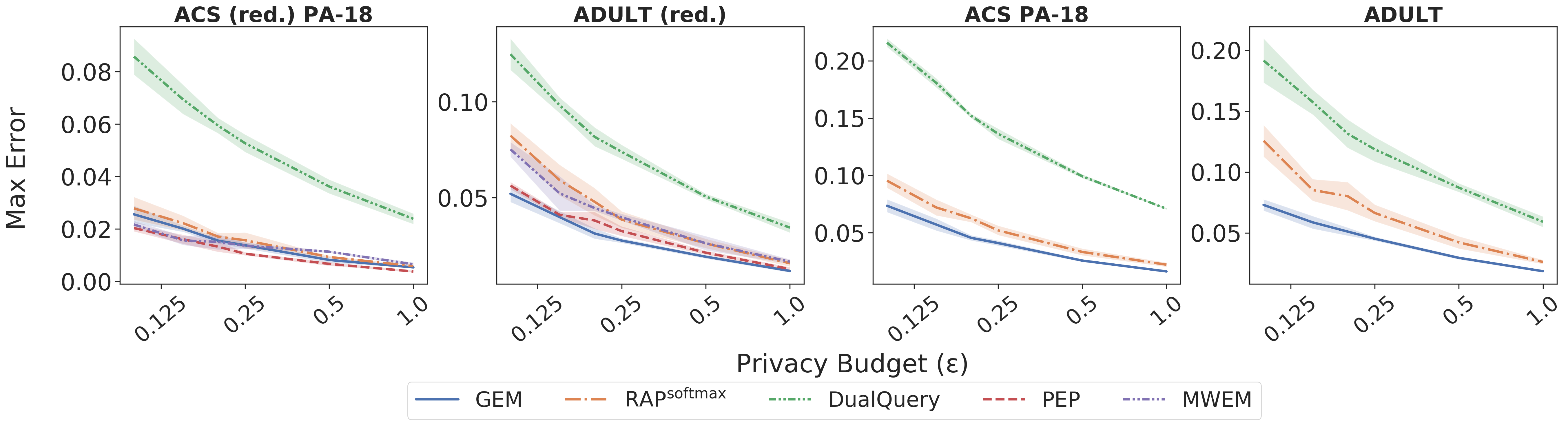
Figure 1: Max error for $3$-way marginals evaluated on ADULT and ACS PA-18 using privacy budgets $\varepsilon\in\{0.1,0.15,0.2,0.25,0.5,1\}$ and $\delta=\frac{1}{n^{2}}$. The x-axis uses a logarithmic scale. We evaluate using the following workload sizes: ACS (reduced) PA-18: $455$; ADULT (reduced): $35$; ACS PA-18: $4096$; ADULT: $286$. Results are averaged over $5$ runs, and error bars represent one standard error.

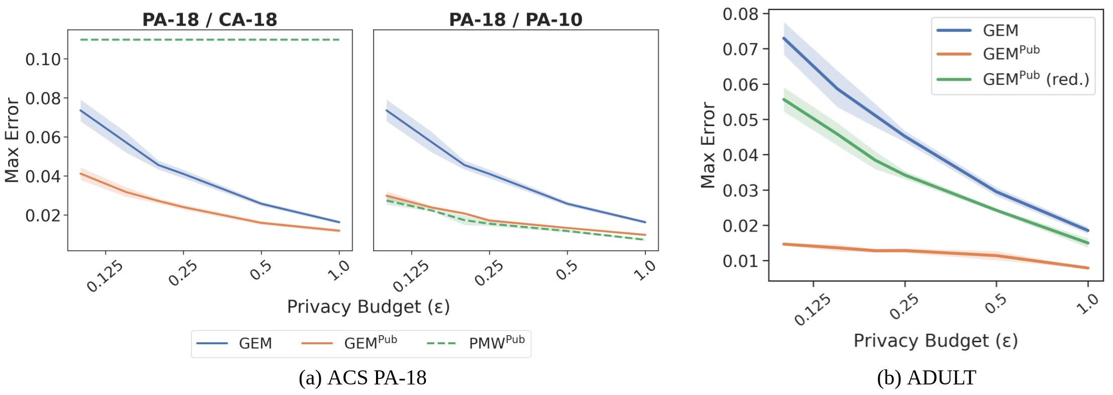
Figure 2: Max error for $3$-way marginals with privacy budgets $\varepsilon\in\{0.1,0.15,0.2,0.25,0.5,1\}$ and $\delta=\frac{1}{n^{2}}$. The x-axis uses a logarithmic scale. Results are averaged over $5$ runs, and error bars represent one standard error. (a) ACS PA-18 (workloads = $4096$). We evaluate public-data-assisted algorithms with the following public datasets: Left: 2018 California (CA-18); Right: 2010 Pennsylvania (PA-10). (b) ADULT (workloads = $286$). We evaluate GEM using both the complete public data (GEM^Pub) and a reduced version that has fewer attributes (GEM^Pub (reduced)) .

7.1 Results

Standard setting. In Figure 1, we observe that in low-dimensional settings, PEP and GEM consistently achieve strong performance compared to the baseline methods. While MWEM and PEP are similar in nature, PEP outperforms MWEM on both datasets across all privacy budgets except $\varepsilon\in\left\{0.1,0.15\right\}$ on ACS (reduced), where the two algorithms perform similarly. In addition, both PEP and GEM outperform RAP^softmax. Moving on to the more realistic setting in which the data dimension is high, we again observe that GEM outperforms RAP^softmax on both datasets.

Public-data-assisted setting.

To evaluate the query release algorithm in the public-data-assisted setting, we present the three following categories of public data:

Public data with sufficient support. To evaluate our methods when the public dataset for ACS PA-18 has low best-mixture-error, we consider the public dataset ACS PA-10. We observe in Figure 1 that GEM^Pub performs similarly to PMW^Pub, with both outperforming GEM (without public data).

Public data with insufficient support. In Figure 2a, we present CA-18 as an example of this failure case in which the best-mixture-error is over $10\%$, and so for any privacy budget, PMW^Pub cannot achieve max errors lower that this value. However, for the reasons described in Section 6.1, GEM^Pub is not restricted by best-mixture-error and significantly outperforms GEM (without public data) when using either public dataset.

Public data with incomplete data domains. To simulate this setting, we construct a reduced version of the public dataset in which we keep only $7$ out of $13$ attributes in ADULT. In this case, $6$ attributes are missing, and so assuming a uniform distribution over the missing attributes would cause the dimension of the approximating distribution $D$ to grow from $\approx 4.4\times 10^{3}$ to a $\approx 3.2\times 10^{9}$. PMW^Pub would be computationally infeasible to run in this case. To evaluate GEM^Pub, we pretrain the generator $G$ using all $3$-way marginals on both the complete and reduced versions of the public dataset and then finetune on the private dataset (we denote these two finetuned networks as GEM^Pub and GEM^Pub (reduced) respectively). We present results in Figure 2b. Given that the public and private datasets are sampled from the same distribution, GEM^Pub unsurprisingly performs extremely well. However, despite only being pretrained on a small fraction of all $3$-way marginal queries ($\approx 20k$ out $334k$), GEM^Pub (reduced) is still able to improve upon the performance of GEM and achieve lower max error for all privacy budgets.

8 Conclusion

In this work, we present a framework that unifies a long line of iterative private query release algorithms by reducing each method to a choice of some distributional family $\mathcal{D}$ and loss function $\mathcal{L}$. We then develop two new algorithms, PEP and GEM, that outperform existing query release algorithms. In particular, we empirically validate that GEM performs very strongly in high dimensional settings (both with and without public data). We note that we chose a rather simple neural network architecture for GEM, and so for future work, we hope to develop architectures more tailored to our problem. Furthermore, we hope to extend our algorithms to other query classes, including mixed query classes and convex minimization problems [jonconvex].

Appendix A Adaptive Measurements

A.1 $k$-way marginals sensitivity

Typically, iterative private query release algorithms assume that the query class $Q$ contains sensitivity $1$ queries [hardt2010multiplicative, gaboardi2014dual, vietri2020new, aydore2021differentially, liu2021leveraging]. However, recall that a $k$-way marginal query is defined by a subset of features $S\subseteq[d]$ and a target value $y\in\prod_{i\in S}\mathcal{X}_{i}$ (Definition 2). Given a feature set $S$ (with $|S|=k$), we can define a workload $W_{S}$ as the set of queries defined over the features in $S$.

$$W_{S}=\left\{q_{S,y}:y\in\prod_{i\in S}\mathcal{X}_{i}\right\}$$

Then for any dataset $D$, the workload’s answer is given by $W_{S}(D)=\{q_{S,y}(D)\}_{y\in\prod_{i\in S}\mathcal{X}_{i}}$, where $W_{S}$ has $\ell_{2}$-sensitivity equal to $\sqrt{2}$. Therefore to achieve more efficient privacy accounting for $k$-way marginals in Adaptive Measurements, we can use the exponential mechanism to select an entire workload $\hat{W}_{S}$ that contains the max error query and then obtain measurements for all queries in $\hat{W}_{S}$ using the Gaussian mechanism, adding noise

$$z\sim\mathcal{N}\left(0,\left(\frac{\sqrt{2}}{n(1-\alpha)\varepsilon_{0}}\right)^{2}\right).$$

to each query in $W_{S}$.

In appendix D.4, we show that using this marginal trick significantly improves the performance of GEM and therefore recommend this type of privacy accounting when designing query release algorithms for $k$-way marginal queries.

A.2 Choices of loss functions and distributional families

We provide additional details about each iterative algorithm, including the loss function $\mathcal{L}$ and and distributional family $\mathcal{D}$ (under the Adaptive Measurements framework).

MWEM from hardt2010simple

The traditional MWEM algorithm samples one query each round, where after $t$ rounds, the set of queries/measurements is $\widetilde{Q}_{t}=\{\widetilde{q}_{1},\ldots,\widetilde{q}_{t}\},\widetilde{A}_{t}=\{\widetilde{a}_{1},\ldots,\widetilde{a}_{t}\}$. Let the $t-1$ previous solutions be $D_{1},\ldots D_{t-1}$. Then MWEM solves an entropy regularized problem in which it finds $D_{t}$ that minimizes the following loss:

$$\mathcal{L}^{\mbox{{\sf MWEM}}}(D,\widetilde{Q}_{1:t},\widetilde{A}_{1:t})=\sum_{i=1}^{t}\sum_{x\in\mathcal{X}}D(x)\widetilde{q}_{i}(x)\left(\widetilde{a}_{i}-\widetilde{q}_{i}(D_{i-1})\right)+\sum_{x\in\mathcal{X}}D(x)\log D(x)$$

We can show that if $D_{t}=\operatorname{\text{arg}\min}_{D\in\Delta(\mathcal{X})}\mathcal{L}^{\mbox{{\sf MWEM}}}(D,\widetilde{Q}_{t},\widetilde{A}_{t})$ then $D_{t}$ evaluates to $D_{t}(x)\propto\exp\left(-\sum_{i=1}^{t}\widetilde{q}_{i}(x)(\widetilde{a}_{i}-\widetilde{q}_{i}(D_{i-1}))\right)$ which is the exactly the distribution computed by MWEM. See A.3 for derivation. We note that MWEM explicitly maintains (and outputs) a distribution $D\in\mathcal{D}$ where $\mathcal{D}$ includes all distributions over the data domain $\mathcal{X}$, making it computationally intractable for high-dimension settings.

DualQuery from gaboardi2014dual

DualQuery is a special case of the Adaptive Measurements framework in which the measurement step is skipped (abusing notation, we say $\alpha=1$). Over all iterations of the algorithm, DualQuery keeps track of a probability distribution over the set of queries $\mathcal{Q}$ via multiplicative weights, which we denote here by $\mathcal{Q}_{t}\in\Delta(Q)$. On round $t$, DualQuery samples $s$ queries ($\widetilde{Q}_{t}=\{\widetilde{q}_{t,1},\ldots\widetilde{q}_{t,s}\}$) from $\mathcal{Q}_{t}$ and outputs $D_{t}$ that minimizes the the following loss function:

$$\mathcal{L}^{\mbox{{\sf DualQuery}}}(D,\widetilde{Q}_{t})=\sum_{i=1}^{s}\widetilde{q}_{t,i}(D)$$

The optimization problem for $\mathcal{L}^{\mbox{{\sf DualQuery}}}(D,\widetilde{Q}_{t})$ is NP-hard. However, the algorithm encodes the problem as a mix-integer-program (MIP) and takes advantage of available fast solvers. The final output of DualQuery is the average $\frac{1}{T}\sum_{t=1}^{T}D_{t}$, which we note implicitly describes some empirical distribution over $\mathcal{X}$.

FEM from vietri2020new

The algorithm FEM follows a follow the perturbed leader strategy. As with MWEM, the algorithm FEM samples one query each round using the exponential mechanism, so that the set of queries in round $t$ is $\widetilde{Q}_{t}=\{\widetilde{q}_{1},\ldots,\widetilde{q}_{t}\}$. Then on round $t$, FEM chooses the next distribution by solving:

$$\mathcal{L}^{\mbox{\sf FEM}}(D,\widetilde{Q}_{1:t})=\sum_{i=1}^{t}\widetilde{q}_{t}(D)+\mathbb{E}_{x\sim D,\eta\sim\text{Exp}(\sigma)^{d}}\left(\langle x,\eta\rangle\right)$$

Similar to DualQuery, the optimization problem for $\mathcal{L}^{\mbox{\sf FEM}}$ also involves solving an NP-hard problem. Additionally, because the function $\mathcal{L}^{\mbox{\sf FEM}}$ does not have a closed form due to the expectation term, FEM follows a sampling strategy to approximate the optimal solution. On each round, FEM generates $s$ samples, where each sample is obtained in the following way: Sample a noise vector $\eta\sim\text{Exp}(\sigma)^{d}$ from the exponential distribution and use a MIP to solve $x_{t,i}\leftarrow\operatorname{\text{arg}\min}_{x\in\mathcal{X}}\sum_{i=1}^{t}\widetilde{q}_{t}(D)+\langle x,\eta\rangle$ for all $i\in[s]$. Finally, the output on round $t$ is the empirical distribution derived from the $s$ samples: $D_{t}=\{x_{t,1},\ldots,x_{t,s}\}$. The final output is the average $\frac{1}{T}\sum_{t=1}^{T}D_{t}$.

RAP^softmax adapted from aydore2021differentially

At iteration $t$, RAP^softmax solves the following optimization problem:

$$\mathcal{L}^{\mbox{{\sf RAP}}}(D,\widetilde{Q}_{1:t},\widetilde{A}_{1:t})=\sum_{i,j}\left(\widetilde{q}_{i,j}(D)-\widetilde{a}_{i,j}\right)^{2}$$

As stated in Section A, we apply the softmax function such that RAP^softmax outputs a synthetic dataset drawn from some probabilistic family of distributions $\mathcal{D}=\left\{\sigma(M)|M\in\mathbb{R}^{n^{\prime}\times d}\right\}$.

A.3 MWEM update

Given the loss function:

$$\mathcal{L}^{\text{\mbox{{\sf MWEM}}}}(D,\widetilde{Q}_{t},\widetilde{A}_{t})=\sum_{i=1}^{t}\sum_{x\in\mathcal{X}}D(x)\widetilde{q}_{i}(x)\left(\widetilde{a}_{i}-\widetilde{q}_{i}(D_{i-1})\right)+\sum_{x\in\mathcal{X}}D(x)\log\left(D(x)\right)$$ (6)

The optimization problem becomes $D_{t}=\operatorname{\text{arg}\min}_{D\in\Delta(\mathcal{X})}\mathcal{L}^{\text{mwem}}(D,\widetilde{Q}_{t},\widetilde{A}_{t})$. The solution $D$ is some distribution, which we can express as a constraint $\sum_{x\in\mathcal{X}}D(x)=1$. Therefore, this problem is a constrained optimization problem. To show that (6) is the MWEM’s true loss function, we can write down the Lagrangian as:

$$\mathcal{L}=\sum_{i=1}^{t}\sum_{x\in\mathcal{X}}D(x)\widetilde{q}_{i}(x)\left(\widetilde{a}_{i}-\widetilde{q}_{i}(D_{i-1})\right)+\sum_{x\in\mathcal{X}}D(x)\log\left(D(x)\right)+\lambda\left(\sum_{x\in\mathcal{X}}D(x)-1\right)$$

Taking partial derivative with respect to $D(x)$:

$$\frac{\partial\mathcal{L}}{\partial D(x)}=\sum_{i=1}^{t}\widetilde{q}_{i}(x)\left(\widetilde{a}_{i}-\widetilde{q}_{i}(D_{i-1})\right)+(1+\log D(x))+\lambda$$

Setting $\frac{\partial\mathcal{L}}{\partial D(x)}=0$ and solving for $D(x)$:

$$D(x)=\exp\left(-1-\lambda-\sum_{i=1}^{t}\widetilde{q}_{i}(x)\left(\widetilde{a}_{i}-\widetilde{q}_{i}(D_{i-1})\right)\right)$$

Finally, the value of $\lambda$ is set such that $D$ is a probability distribution:

$$D(x)=\frac{\exp\left(-\sum_{i=1}^{t}\widetilde{q}_{i}(x)\left(\widetilde{a}_{i}-\widetilde{q}_{i}(D_{i-1})\right)\right)}{\sum_{x\in\mathcal{X}}\exp\left(-\sum_{i=1}^{t}\widetilde{q}_{i}(x)\left(\widetilde{a}_{i}-\widetilde{q}_{i}(D_{i-1})\right)\right)}$$

This concludes the derivation of MWEM loss function.

Appendix B GEM

We show the exact details of GEM in Algorithms 2 and 3. Note that given a vector of queries $Q_{t}=\left\langle q_{1},\ldots,q_{t}\right\rangle$, we define $f_{Q_{t}}(\cdot)=\left\langle f_{q_{1}}(\cdot),\ldots,f_{q_{t}}(\cdot)\right\rangle$.

Input: Private dataset $P$, set of differentiable queries $Q$

Parameters: privacy parameter $\rho$, number of iterations $T$, privacy weighting parameter $\alpha$, batch size $B$, stopping threshold $\gamma$

Initialize generator network $G_{0}$

Let $\varepsilon_{0}=\sqrt{\frac{2\rho}{T\left(\alpha^{2}+\left(1-\alpha\right)^{2}\right)}}$  

for $t=1\ldots T$ do

       Sample: Sample $\mathbf{z}=\left\langle z_{1}\ldots z_{B}\right\rangle\sim\mathcal{N}(0,I_{B})$

       Choose $\widetilde{q}_{t}$ using the exponential mechanism with score

$$\mathrm{Pr}\left[q_{t}=q\right]\propto\exp\left(\frac{\alpha\varepsilon_{0}n}{2}|q(P)-q(G_{t-1}\left(\mathbf{z}\right))|\right)$$

      

      Measure: Let $\widetilde{a}_{t}=\widetilde{q}_{t}(P)+\mathcal{N}\left(0,\left(\frac{1}{n(1-\alpha)\varepsilon_{0}}\right)^{2}\right)$

      

      Update: $G_{t}=\mbox{{\sf GEM-UPDATE}}\left(G_{t-1},Q_{t},\mathbf{\widetilde{a}_{t}},\gamma\right)$ where $Q_{t}=\left\langle\widetilde{q}_{1},\ldots,\widetilde{q}_{t}\right\rangle$ and $\mathbf{\widetilde{a}_{t}}=\left\langle\widetilde{a}_{1},\ldots,\widetilde{a}_{t}\right\rangle$

      

end for

Let $\theta_{out}=\mbox{{\sf EMA}}\left(\left\{\theta_{j}\right\}_{j=\frac{T}{2}}^{T}\right)$ where $\theta_{j}$ parameterizes $G_{j}$

Let $G_{out}$ be the generator parameterized by $\theta_{out}$

Output $G_{out}\left(\mathbf{z}\right)$

Algorithm 2 GEM

Input: Generator $G$ parameterized by $\theta$, queries $Q$, noisy measurements $\mathbf{\widetilde{a}}$, stopping threshold $\gamma$

Parameters: max iterations $T_{\text{max}}$, batch size $B$

Sample $\mathbf{z}=\left\langle z_{1}\ldots z_{B}\right\rangle\sim\mathcal{N}(0,I_{B})$

Let $\mathbf{c}=\mathbf{\widetilde{a}}-\frac{1}{B}\sum_{j=1}^{B}f_{Q}\left(G\left(z_{j}\right)\right)$ be errors over queries $Q$

Let $i=0$

while $i<T_{\text{max}}$ and $\lVert\mathbf{c}\rVert_{\infty}\geq\gamma$ do

       Let $J=\left\{j\mid|c_{j}|\geq\gamma\right\}$

       Update $G$ to minimize the loss function with the stochastic gradient $\nabla_{\theta}\frac{1}{|J|}\sum_{j\in J}|c_{ij}|$

       Sample $\mathbf{z}=\left\langle z_{1}\ldots z_{B}\right\rangle\sim\mathcal{N}(0,I_{B})$

       Let $\mathbf{c}=\mathbf{\widetilde{a}}-\frac{1}{B}\sum_{j=1}^{B}f_{Q}\left(G\left(z_{j}\right)\right)$

       Let $i=i+1$

      

end while

Output: $G$

Algorithm 3 GEM-UPDATE

B.1 Loss function (for $k$-way marginals) and distributional family

For any $z\in\mathbb{R}$, $G(z)$ outputs a distribution over each attribute, which we can use to calculate the answer to a query via $f_{q}$. In GEM however, we instead sample a noise vector $\mathbf{z}=\left\langle z_{1}\ldots z_{B}\right\rangle$ and calculate the answer to some query $q$ as $\frac{1}{B}\sum_{j=1}^{B}f_{q}\left(G\left(z_{j}\right)\right)$. One way of interpreting the batch size $B$ is to consider each $G\left(z_{j}\right)$ as a unique distribution. In this sense, GEM models $B$ sub-populations that together comprise the overall population of the synthetic dataset. Empirically, we find that our model tends to better capture the distribution of the overall private dataset in this way (Figure 3). Note that for our experiments, we choose $B=1000$ since it performs well while still achieving good running time. However, this hyperparameter can likely be further increased or tuned (which we leave to future work).

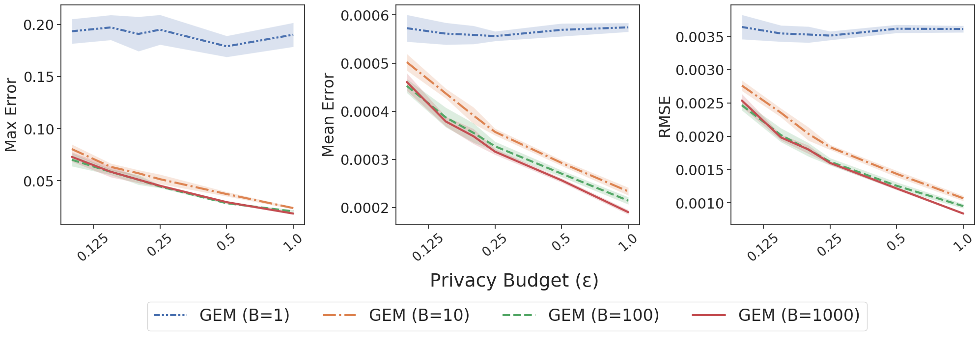
Figure 3: Error comparison of GEM using different batch sizes $B$ on ADULT (workloads=286), evaluated on $3$-way marginals with privacy budgets $\varepsilon\in\{0.1,0.15,0.2,0.25,0.5,1\}$ and $\delta=\frac{1}{n^{2}}$. The x-axis uses a logarithmic scale. Results are averaged over $5$ runs, and error bars represent one standard error.

Therefore, using this notation, GEM outputs then a generator $G\in\mathcal{D}$ by optimizing $\ell_{1}$-loss at each step $t$ of the Adaptive Measurements framework:

$$\mathcal{L}^{\mbox{{\sf GEM}}}\left(G,\widetilde{Q}_{1:t},\widetilde{A}_{1:t}\right)=\sum_{i=1}^{t}\left|\frac{1}{B}\sum_{j=1}^{B}f_{\widetilde{q}_{i}}\left(G\left(z_{j}\right)\right)-\widetilde{a}_{i}\right|$$ (7)

Lastly, we note that we can characterize family of distributions $\mathcal{D}=\left\{G_{\theta}(z)|z\sim\mathcal{N}(0,1)\right\}$ in GEM by considering it as a class of distributions whose marginal densities are parameterized by $\theta$ and Gaussian noise $z\sim\mathcal{N}(0,1)$ We remark that such densities can technically be characterized as Boltzmann distributions.

B.2 Additional implementation details

EMA output

We observe empirically that the performance of the last generator $G_{T}$ is often unstable. One possible solution explored previously in the context of privately trained GANs is to output a mixture of samples from a set of generators [beaulieu2019privacy, neunhoeffer2020private]. In our algorithm GEM, we instead draw inspiration from yazici2018unusual and output a single generator $G_{out}$ whose weights $\theta_{out}$ are an exponential moving average (EMA) of weights $\theta_{t}$ obtained from the latter half of training. More concretely, we define $\theta_{out}=\mbox{{\sf EMA}}\left(\left\{\theta_{j}\right\}_{j=\frac{T}{2}}^{T}\right)$, where the update rule for EMA is given by $\theta^{EMA}_{k}=\beta\theta^{EMA}_{k-1}+(1-\beta)\theta_{k}$ for some parameter $\beta$.

Stopping threshold $\gamma$

To reduce runtime and prevent GEM from overfitting to the sampled queries, we run GEM-UPDATE with some early stopping threshold set to an error tolerance $\gamma$. Empirically, we find that setting $\gamma$ to be half of the max error at each time step $t$. Because sampling the max query using the exponential mechanism provides a noisy approximation of the true max error, we find that using an exponential moving average (with $\beta=0.5$) of the sampled max errors is a more stable approximation of the true max error. More succinctly, we set $\gamma=\mbox{{\sf EMA}}(\left\{c_{i}\right\}_{i=0}^{t})$ where $c_{i}$ is max error at the beginning of iteration $i$.

Resampling Gaussian noise.

In our presentation of GEM and in Algorithms 2 and 3, we assume that GEM resamples Gaussian noise $z$. While resampling $z$ encourages GEM to train a generator to output a distribution for any $\mathbf{z}\sim\mathcal{N}(0,I_{B})$ for some fixed batch size $B$, we find that fixing the noise vector $\mathbf{z}$ at the beginning of training leads to faster convergence. Moreover in Figure 4, we show that empirically, the performance between whether we resample $z$ at each iteration is not very different. Since resampling $z$ does not induce any benefits to generating synthetic data for the purpose of query release, in which the goal is output a single synthetic dataset or distribution, we run all experiments without resampling $z$. However, we note that it is possible that in other settings, resampling the noise vector at each step makes more sense and warrants compromising per epoch convergence speed and overall runtime. We leave further investigation to future work.

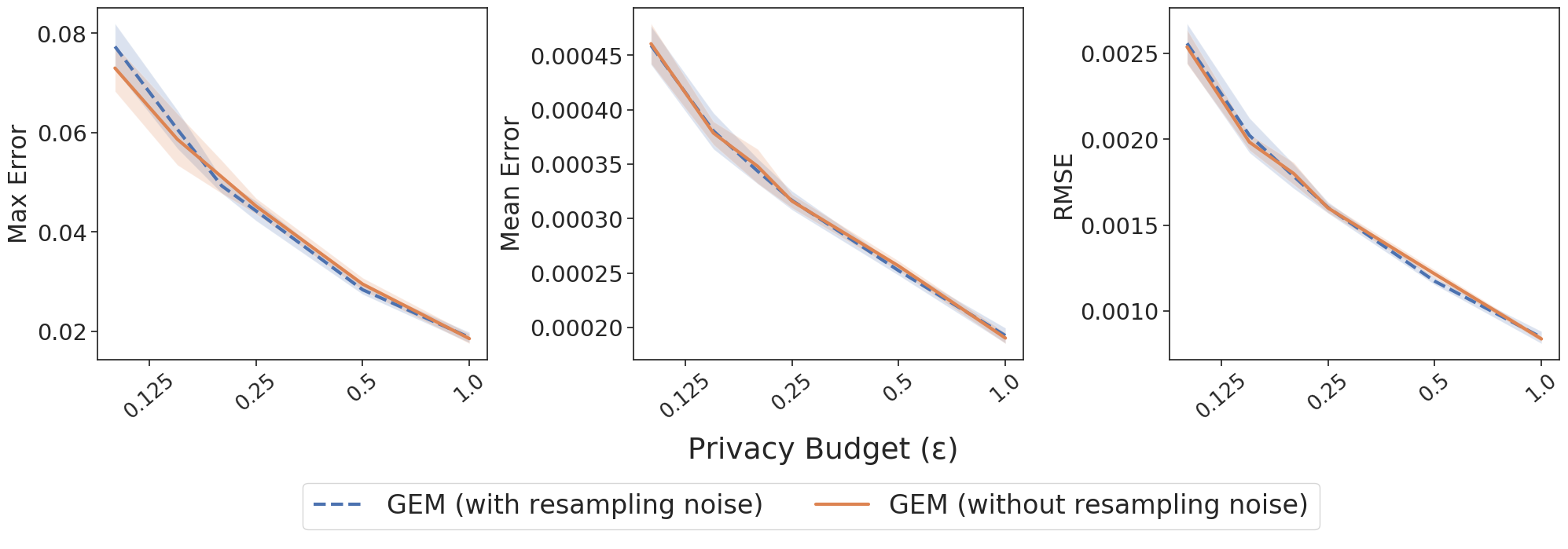
Figure 4: Error comparison of GEM with and without resampling $\mathbf{z}$ at each step on ADULT (workloads=286), evaluated on $3$-way marginals with privacy budgets $\varepsilon\in\{0.1,0.15,0.2,0.25,0.5,1\}$ and $\delta=\frac{1}{n^{2}}$. The x-axis uses a logarithmic scale. Results are averaged over $5$ runs, and error bars represent one standard error.

B.3 Optimizing over arbitrary query classes

To optimize the loss function for GEM (Equation 4) using gradient-based optimization, we need to have access to the gradient of each $\widetilde{q}_{i}$ with respect to the input distribution $G_{\theta}(z)$ for any $z$ (once we compute this gradient, we can then derive the gradient of the loss function with respect to the parameters $\theta$ via chain rule). Given any arbitrary query function $q$, we can rewrite it as (3), which is differentiable w.r.t. $\theta$.

More specifically, for $\mathbf{z}\sim N(0,I_{k})$, we write $P_{\theta}(x)=\mathbb{E}_{\mathbf{z}\sim N(0,I_{k})}\left[P_{\theta,\mathbf{z}}(x)\right]$, where

$$P_{\theta,\mathbf{z}}(x)=\frac{1}{k}\sum_{i=1}^{k}\prod_{j=1}^{d^{\prime}}(G_{\theta}(z_{i})_{j})^{x_{j}}$$

Then

$$\nabla_{\theta}[q(P_{\theta})] =\nabla_{\theta}\sum_{x\in\mathcal{X}}\phi(x)P_{\theta}(x)$$

$$=\sum_{x\in\mathcal{X}}\phi(x)\nabla_{\theta}P_{\theta}(x)$$

$$=\sum_{x\in\mathcal{X}}\phi(x)\nabla_{\theta}\left[\mathbb{E}_{\mathbf{z}\sim N(0,I_{k})}\left[P_{\theta,\mathbf{z}}(x)\right]\right]$$

$$=\mathbb{E}_{\mathbf{z}\sim N(0,I_{k})}\left[\sum_{x\in\mathcal{X}}\phi(x)\nabla_{\theta}\left[P_{\theta,\mathbf{z}}(x)\right]\right]$$

However, while this form allows us to compute the gradient $\nabla_{\theta}q$ even when $\phi$ itself may not be differentiable w.r.t. $x$ or have a closed form, this method is not computationally feasible when the data domain $\mathcal{X}$ is too large because it requires evaluating $\phi$ on all $x\in\mathcal{X}$. One possible alternative is to construct an unbiased estimator. However, this estimator may suffer from high variance when the number of samples is insufficiently large, inducing a trade-off between computational efficiency and the variance of the estimator.

Incorporating techniques from reinforcement learning, such as the REINFORCE algorithm [williams1992simple], may serve as alternative ways for optimizing over non-differentiable queries. Specifically, we can approximate (3) in the following way:

$$\nabla_{\theta}[q(P_{\theta})] =\mathbb{E}_{\mathbf{z}\sim N(0,I_{k})}\left[\sum_{x\in\mathcal{X}}\phi(x)\nabla_{\theta}P_{\theta,\mathbf{z}}(x)\right]$$

$$=\mathbb{E}_{\mathbf{z}\sim N(0,I_{k})}\left[\sum_{x\in\mathcal{X}}\phi(x)\frac{P_{\theta,\mathbf{z}}}{P_{\theta,\mathbf{z}}}\nabla_{\theta}P_{\theta,\mathbf{z}}(x)\right]$$

$$=\mathbb{E}_{\mathbf{z}\sim N(0,I_{k})}\left[\sum_{x\in\mathcal{X}}\phi(x)P_{\theta,\mathbf{z}}(x)\nabla_{\theta}\log P_{\theta,\mathbf{z}}(x)\right]$$

We can then approximate this gradient by drawing $m$ samples $\{x_{1}\ldots x_{m}\}$ from $P_{\theta,\mathbf{z}}(x)$, giving us

$$\mathbb{E}_{\mathbf{z}\sim N(0,I_{k})}\left[\frac{1}{m}\sum_{i=1}^{k}\phi(x_{i})\nabla_{\theta}\log P_{\theta,\mathbf{z}}(x_{i})\right]$$

Further work would be required to investigate whether optimizing such surrogate loss functions is effective when differentiable, closed-form representations of a given query class (e.g., the product query representation of $k$-way marginals) are unavailable.

Appendix C PEP

In the following two sections, we first derive PEP’s loss function and and in the next section we derive PEP’s update rule (or optimization procedure) that is used to minimize it’s loss function.

C.1 PEP loss function

In this section we derive the loss function that algorithm PEP optimizes over on round $t$. Fixing round $t$, we let $\widetilde{Q}_{t}\subset Q$ be a subset of queries that were selected using a private mechanism and and let $\widetilde{A}_{t}$ be the noisy measurements corresponding to $\widetilde{Q}_{t}$. Then algorithm PEP finds a feasible solution to the problem:

minimize: $$\text{RE}\left(D\parallel U\right)$$ (8)

subject to: $$\forall_{i\in[t]}\quad\left|\widetilde{a}_{i}-\widetilde{q}_{i}(D)\right|\leq\gamma,\quad\sum_{x\in\mathcal{X}}D(x)=1$$

The Lagrangian of (8) is :

$$\mathcal{L} =\text{RE}\left(D\parallel U\right)+\sum_{i=1}^{t}\lambda_{i}^{+}\left(\widetilde{a}_{i}-\widetilde{q}_{i}(D)-\gamma\right)+\sum_{i=1}^{t}\lambda_{i}^{-}\left(\widetilde{q}_{i}(D)-\widetilde{a}_{i}-\gamma\right)+\mu\left(\sum_{x}D(x)-1\right)$$

Let $\lambda\in\mathbb{R}^{t}$ be a vector with, $\lambda_{i}=\lambda_{i}^{-}-\lambda_{i}^{+}$. Then

$$\mathcal{L}=\text{RE}\left(D\parallel U\right)+\sum_{i=1}^{t}\lambda_{i}\widetilde{q}_{i}(D)-\sum_{i=1}^{t}\lambda_{i}\widetilde{a}_{i}-\gamma\sum_{i=1}^{t}\left(\lambda_{i}^{+}+\lambda_{i}^{-}\right)+\mu\left(\sum_{x}D(x)-1\right)$$ (9)

where $\|\lambda\|_{1}=\sum_{i=1}^{t}\left(\lambda_{i}^{+}+\lambda_{i}^{-}\right)$. Taking the derivative with respect to $D(x)$ and setting to zero, we get:

$$0=\frac{\partial\mathcal{L}}{\partial D(x)} =\log\left(\frac{D(x)}{U(x)}\right)+1+\sum_{i=1}^{t}\lambda_{i}\widetilde{q}_{i}(x)+\mu$$

Solving for $D(x)$, we get

$$D(x)=U(x)\exp\left(-\sum_{i=1}^{t}\lambda_{i}\widetilde{q}_{i}(x)-\mu-1\right)$$

The slack variable $\mu$ must be selected to satisfy the constraint that $\sum_{x\in\mathcal{X}}D(x)=1$. Therefore have that the solution to (8) is a distribution parameterized by the parameter $\lambda$, such that for any $x\in\mathcal{X}$ we have

$$D(x)=\frac{U(x)}{Z}\exp\left(-\sum_{i=1}^{t}\lambda_{i}\widetilde{q}_{i}(x)\right)$$

where $Z=\sum_{x\in\mathcal{X}}U(x)\exp\left(-\sum_{i=1}^{t}\lambda_{i}\widetilde{q}_{i}(x)\right)$. Plugging into (9), we get

$$\mathcal{L} =\sum_{x\in\mathcal{X}}D(x)\log\left(\frac{D(x)}{U(x)}\right)+\sum_{i=1}^{t}\lambda_{i}\widetilde{q}_{i}(D)-\sum_{i=1}^{t}\lambda_{i}\widetilde{a}_{i}-\gamma\|\lambda\|_{1}$$

$$=\sum_{x\in\mathcal{X}}D(x)\left(-\sum_{i=1}^{t}\lambda_{i}\widetilde{q}_{i}(x)\right)-\log(Z)+\sum_{i=1}^{t}\lambda_{i}\widetilde{q}_{i}(D)-\sum_{i=1}^{t}\lambda_{i}\widetilde{a}_{i}-\gamma\|\lambda\|_{1}$$

$$=-\sum_{i=1}^{t}\lambda_{i}\widetilde{q}_{i}(D)-\log(Z)+\sum_{i=1}^{t}\lambda_{i}\widetilde{q}_{i}(D)-\sum_{i=1}^{t}\lambda_{i}\widetilde{a}_{i}-\gamma\|\lambda\|_{1}$$

$$=-\log(Z)+\sum_{i=1}^{t}\lambda_{i}\widetilde{a}_{i}-\gamma\|\lambda\|_{1}$$

$$=-\log\left(\frac{Z}{\exp\left(\sum_{i=1}^{t}\lambda_{i}\widetilde{a}_{i}\right)}\right)-\gamma\|\lambda\|_{1}$$

Substituting in for $Z$, we get:

$$\mathcal{L} =-\log\left(\frac{\sum_{x\in\mathcal{X}}\exp\left(\sum_{i=1}^{t}\lambda_{i}\widetilde{q}_{i}(x)\right)}{\exp\left(\sum_{i=1}^{t}\lambda_{i}\widetilde{a}_{i}\right)}\right)-\gamma\|\lambda\|_{1}$$

$$=-\log\left(\sum_{x\in\mathcal{X}}\exp\left(\sum_{i=1}^{t}\lambda_{i}\left(\widetilde{q}_{i}(x)-\widetilde{a}_{i}+\gamma\right)\right)\right)-\gamma\|\lambda\|_{1}$$

Finally, we have that the dual problem of (8) finds a vector $\lambda=(\lambda_{1},\ldots,\lambda_{t})$ that maximizes $\mathcal{L}$. We can write the dual problem as a minimization problem:

$$\mathcal{L}(\lambda)=\min_{\lambda}\log\left(\sum_{x\in\mathcal{X}}\exp\left(\sum_{i=1}^{t}\lambda_{i}\left(\widetilde{q}_{i}(x)-\widetilde{a}_{i}\right)\right)\right)+\gamma\|\lambda\|_{1}$$

C.2 PEP optimization using iterative projection

In this section we derive the update rule in algorithm 4. Recall that the ultimate goal is to solve (8). Before we describe the algorithm, we remark that it is possible the constraints in problem 8 cannot be satisfied due to the noise we add to the measurements $\widetilde{a}_{1},\ldots\widetilde{a}_{t}$. In principle, $\gamma$ can be chosen to be a high-probability upper bound on the noise, which can be calculated through standard concentration bounds on Gaussian noise. In that case, every constraint $|\widetilde{a}_{i}-\widetilde{q}_{i}(D)|\leq\gamma$ can be satisfied and the optimization problem is well defined. However, we note that our algorithm is well defined for every choice of $\gamma\geq 0$. For example, in our experiments we have $\gamma=0$, and we obtain good empirical results that outperform MWEM. In this section we assume that $\gamma=0$.

To explain how algorithm 4 converges, we cite an established convergence analysis of adaboost from [schapire2013boosting, chapter 7] . Similar to adaboost, Algorithm 2 is running iterative projection, where on each iteration, it projects the distribution to satisfy a single constraint. As shown in [schapire2013boosting, chapter 7], this iterative algorithm converges to a solution that satisfies all the constraints. The PEP algorithm can be seen as an adaptation of the adaboost algorithm to the setting of query release. Therefore, to solve (8), we use an iterative projection algorithm that on each round selects an unsatisfied constraint and moves the distribution by the smallest possible distance to satisfy it.

Let $\widetilde{Q}_{1:t}$ and $\widetilde{A}_{1:t}$ be the set of queries and noisy measurements obtained using the private selection mechanism. Let $K$ be the number of iterations during the optimization and let $D_{t,0},\ldots,D_{t,K}$ be the sequence of projections during the $K$ iteration of optimization. The goal is that $D_{t,K}$ matches all the constraints defined by $\widetilde{Q}_{1:t}$, $\widetilde{A}_{1:t}$. Our initial distribution is the uniform distribution $D_{t,0}=U$. Then on round $k\in[K]$, the algorithm selects an index $i_{k}\in[t]$ such that the $i_{k}$-th constraint has high error on the current distribution $D_{t,k-1}$. Then the algorithm projects the distribution such that the $i_{k}$-th constraint is satisfied and the distance to $D_{t,k-1}$ is minimized. Thus, the objective for iteration $k$ is:

minimize: $$\text{RE}\left(D\parallel D_{t,k-1}\right) \quad\widetilde{a}_{i_{k}}=\widetilde{q}_{i_{k}}(D),\quad\sum_{x\in\mathcal{X}}D(x)=1$$ subject to: (10)

Input: Error tolerance $\gamma$, linear queries $\widetilde{Q}_{1:T}=\{\widetilde{q}_{1},\ldots,\widetilde{q}_{T}\}$, and noisy measurements $\widetilde{A}_{1:T}=\{\widetilde{a}_{1},\ldots,\widetilde{a}_{T}\}$.

Objective: Minimize $\text{RE}\left(D\parallel U\right)$ such that $\forall_{i\in[T]}\quad\left|\widetilde{q}_{i}(D)-\widetilde{a}_{i}\right|\leq\gamma$.

Initialize $D_{0}$ to be the uniform distribution over $\mathcal{X}$, and $t\leftarrow 0$.

while $\max_{i\in[T]}\left|\widehat{a}_{i}-\widetilde{q}_{i}(D_{t})\right|>\gamma$  do

       Choose: $i\in[T]$ with $i\leftarrow\operatorname{\text{arg}\max}_{j\in[T]}\left|\widetilde{a}_{j}-\widetilde{q}_{j}(D_{t})\right|$.

       Update: For all $x\in\mathcal{X}$, set $D_{t+1}(x)\leftarrow D_{t}(x)e^{-\lambda_{t}\widetilde{q}_{i}(x)}$, where $-\lambda_{t}=\ln\left(\frac{\widetilde{a}_{i}(1-\widetilde{q}_{i}(D_{t}))}{(1-\widetilde{a}_{i})\widetilde{q}_{i}(D_{t})}\right)$.

       $t\leftarrow t+1$

      

end while

Output: $D_{T}$

Algorithm 4 Exponential Weights Projection

Then the Lagrangian of objective (10) is:

$$\mathcal{L}(D,\lambda)=\text{RE}\left(D\parallel D_{k-1}\right)+\lambda\left(\widetilde{q}_{i_{k}}(D)-\widetilde{a}_{i_{k}}\right)+\mu\left(\sum_{x\in\mathcal{X}}D(x)-1\right)$$ (11)

Taking the partial derivative with respect to $D(x)$, we have

$$\frac{\partial\mathcal{L}(D,\lambda)}{\partial D(x)}=\ln\left(\frac{D(x)}{D_{k-1}(x)}\right)+1+\lambda\widetilde{q}_{i_{k}}(x)+\mu=0$$ (12)

Solving (12) for $D(x)$, we get

$$D(x)=D_{k-1}(x)\exp\left(-\lambda\widetilde{q}_{i_{k}}(x)-1-\mu\right)=\tfrac{D_{k-1}(x)}{Z}\exp\left(-\lambda\widetilde{q}_{i_{k}}(x)\right)$$ (13)

where $\mu$ is chosen to satisfy the constraint $\sum_{x\in\mathcal{X}}D(x)=1$ and $Z$ is a regularization factor. Plugging (13) into (11), we get:

$$\mathcal{L}(D,\lambda) =\text{RE}\left(D\parallel D_{k-1}\right)+\lambda\left(\widetilde{q}_{i_{k}}(D)-\widetilde{a}_{i_{k}}\right)$$

$$=\sum_{x}D(x)\log\left(\frac{D(x)}{D_{k-1}(x)}\right)+\lambda\left(\widetilde{q}_{i_{k}}(D)-\widetilde{a}_{i_{k}}\right)$$

$$=\sum_{x}D(x)\log\left(\frac{1}{Z}\frac{D_{k-1}(x)e^{-\lambda q_{i_{k}}(x)}}{D_{k-1}(x)}\right)+\lambda\left(\widetilde{q}_{i_{k}}(D)-\widetilde{a}_{i_{k}}\right)$$ (13)

$$=-\lambda\sum_{x}D(x)\widetilde{q}_{i_{k}}(x)-\log(Z)+\lambda\left(\widetilde{q}_{i_{k}}(D)-\widetilde{a}_{i_{k}}\right)$$

$$=-\lambda\widetilde{q}_{i_{k}}(D)-\log(Z)+\lambda\left(\widetilde{q}_{i_{k}}(D)-\widetilde{a}_{i_{k}}\right)$$

$$=-\log(Z)-\lambda\widetilde{a}_{i_{k}}$$

$$=-\log\left(\sum_{x\in\mathcal{X}}D_{k-1}(x)\exp\left(-\lambda\widetilde{q}_{i_{k}}(x)\right)\right)-\lambda\widetilde{a}_{i_{k}}$$

The next step is to find the optimal value of $\lambda$. Therefore we calculate the derivative of $\mathcal{L}(D,\lambda)$ with respect to $\lambda$:

$$\frac{\partial\mathcal{L}(D,\lambda)}{\partial\lambda} =\frac{e^{-\lambda}\widetilde{q}_{i_{k}}(D_{k-1})}{\sum_{x\in\mathcal{X}}D_{k-1}(x)\exp\left(-\lambda\widetilde{q}_{i_{k}}(x)\right)}-\widetilde{a}_{i_{k}}$$

$$=\frac{e^{-\lambda}\widetilde{q}_{i_{k}}(D_{k-1})}{e^{-\lambda}\widetilde{q}_{i_{k}}(D_{k-1})+(1-\widetilde{q}_{i_{k}}(D_{k}))}-\widetilde{a}_{i_{k}}$$

Setting $\frac{\partial\mathcal{L}(D,\lambda)}{\partial\lambda}=0$, we can solve for $\lambda$.

$$\frac{e^{-\lambda}\widetilde{q}_{i_{k}}(D_{k-1})}{e^{-\lambda}\widetilde{q}_{i_{k}}(D_{k-1})+(1-\widetilde{q}_{i_{k}}(D_{k}))} =\widetilde{a}_{i_{k}}$$

$$e^{-\lambda}\widetilde{q}_{i_{k}}(D_{k-1}) =\widetilde{a}_{i_{k}}\left(e^{-\lambda}\widetilde{q}_{i_{k}}(D_{k-1})+(1-\widetilde{q}_{i_{k}}(D_{k}))\right)$$

$$e^{-\lambda}\widetilde{q}_{i_{k}}(D_{k-1})-e^{-\lambda}\widetilde{a}_{i_{k}}\widetilde{q}_{i_{k}}(D_{k-1}) =\widetilde{a}_{i_{k}}\left(1-\widetilde{q}_{i_{k}}(D_{k})\right)$$

$$e^{-\lambda}\widetilde{q}_{i_{k}}(D_{k-1})\left(1-\widetilde{a}_{i_{k}}\right) =\widetilde{a}_{i_{k}}\left(1-\widetilde{q}_{i_{k}}(D_{k})\right)$$

Finally we obtain

$$-\lambda=\ln\left(\frac{\widetilde{a}_{i_{k}}\left(1-\widetilde{q}_{i_{k}}(D_{k-1})\right)}{(1-\widetilde{a}_{i_{k}})\widetilde{q}_{i_{k}}(D_{k-1})}\right)$$

Appendix D Additional empirical evaluation

D.1 Experimental details

We present hyperparameters used for methods across all experiments in Tables 1, 2, 3, 4, and 5. To limit the runtime of PEP and PEP^Pub, we add the hyperparameter, $T_{max}$, which controls the maximum number of update steps taken at each round $t$. Our implementations of MWEM, DualQuery, and PMW^Pub are adapted from https://github.com/terranceliu/pmw-pub. We implement RAP and RAP^softmax ourselves using PyTorch since the code for RAP. All experiments are run using a desktop computer with an Intel® Core™ i5-4690K processor and NVIDIA GeForce GTX 1080 Ti graphics card.

We obtain the ADULT and ACS datasets by following the instructions outlined in https://github.com/terranceliu/pmw-pub. Our version of ADULT used to train GEM^Pub (reduced) (Figure 2b and 7) uses the following attributes: sex, race, relationship, marital-status, occupation, education-num, age.

Table 1: PEP hyperparameters

Dataset	Parameter	Values
All	$T_{max}$	$25$
ACS (red.)	$T$	$20$, $30$, $40$, $50$, $75$
		$100$, $125$, $150$, $175$, $200$
ADULT (red.)	$T$	$20$, $30$, $40$, $50$, $75$
		$100$, $125$, $150$, $175$, $200$

Table 2: GEM hyperparameters

Dataset	Parameter	Values
All	hidden layer sizes	$(512,1024,1024)$
	learning rate	$0.0001$
	$B$	$1000$
	$\alpha$	$0.67$
	$T_{max}$	$100$
ACS	$T$	$100$, $150$, $200$, $250$, $300$,
		$400$, $500$, $750$, $1000$
ACS (red.)	$T$	$50$, $75$, $100$, $125$, $150$,
		$200$, $250$, $300$
ADULT, ADULT (red.),	$T$	$30$, $40$, $50$, $60$, $70$,
ADULT (orig),		$80$, $90$, $100$, $125$, $150$,
LOANS		$175$, $200$

Table 3: PEP^Pub hyperparameters

Dataset	Parameter	Values
All	$T_{max}$	$25$
ACS	$T$	$20$, $40$, $60$, $80$, $100$
		$120$, $140$, $160$, $180$, $200$

Table 4: GEM^Pub hyperparameters

Dataset	Parameter	Values
All	hidden layer sizes	$(512,1024,1024)$
	learning rate	$0.0001$
	$B$	$1000$
	$\alpha$	$0.67$
	$T_{max}$	$100$
ACS	$T$	$30$, $40$, $50$, $75$, $100$,
		$150$, $200$, $300$, $400$, $500$
ADULT	$T$	$2$, $3$, $5$, $10$, $20$, $30$, $40$, $50$,
		$60$ $70$ $80$ $90$ $100$

Table 5: Baseline hyperparameters

Method	Parameter	Values
RAP	learning rate	$0.001$
	$n^{\prime}$	$1000$
	$K$	$5$, $10$, $25$, $50$, $100$
	$T$	$2$, $5$, $10$, $25$, $50$, $75$, $100$
RAPsoftmax	learning rate	$0.1$
	$n^{\prime}$	$1000$
	$K$	$5$, $10$, $25$, $50$, $100$
	$T$	$2$, $5$, $10$, $25$, $50$, $75$, $100$
MWEM	$T$	$100$, $150$, $200$, $250$, $300$
		$400$, $500$, $750$, $1000$
MWEM (/w past queries)	$T$	$50$, $75$, $100$, $150$, $200$, $250$, $300$
DualQuery	$\eta$	$2$, $3$, $4$, $5$
	samples	$25$ $50$, $100$, $250$, $500$

D.2 Main experiments with additional metrics

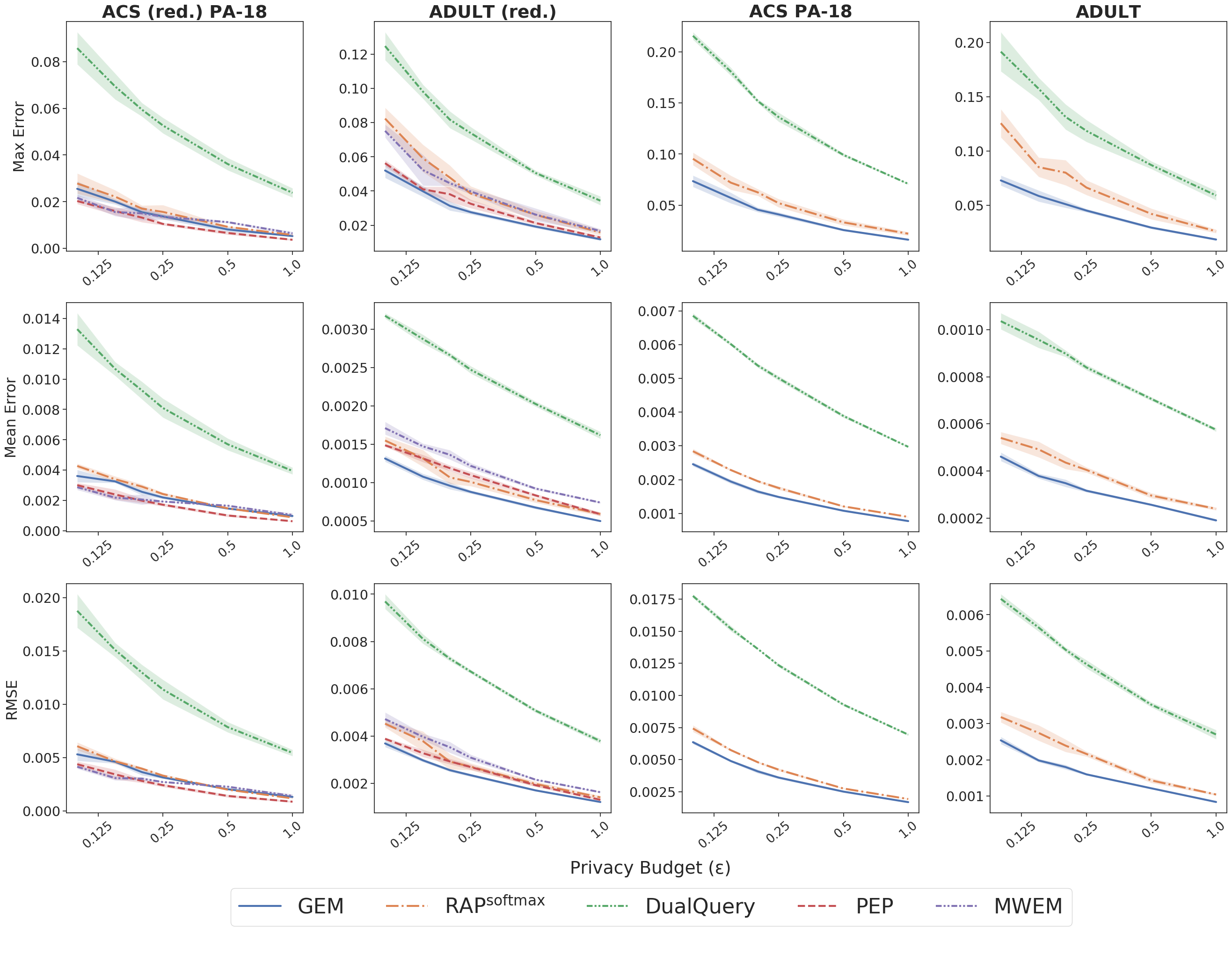
Figure 5: Max, mean, and root mean squared errors for $3$-way marginals evaluated on ADULT and ACS PA-18 using privacy budgets $\varepsilon\in\{0.1,0.15,0.2,0.25,0.5,1\}$ and $\delta=\frac{1}{n^{2}}$. The x-axis uses a logarithmic scale. We evaluate using the following workload sizes: ACS (reduced) PA-18: $455$; ADULT (reduced): $35$; ACS PA-18: $4096$; ADULT: $286$. Results are averaged over $5$ runs, and error bars represent one standard error.

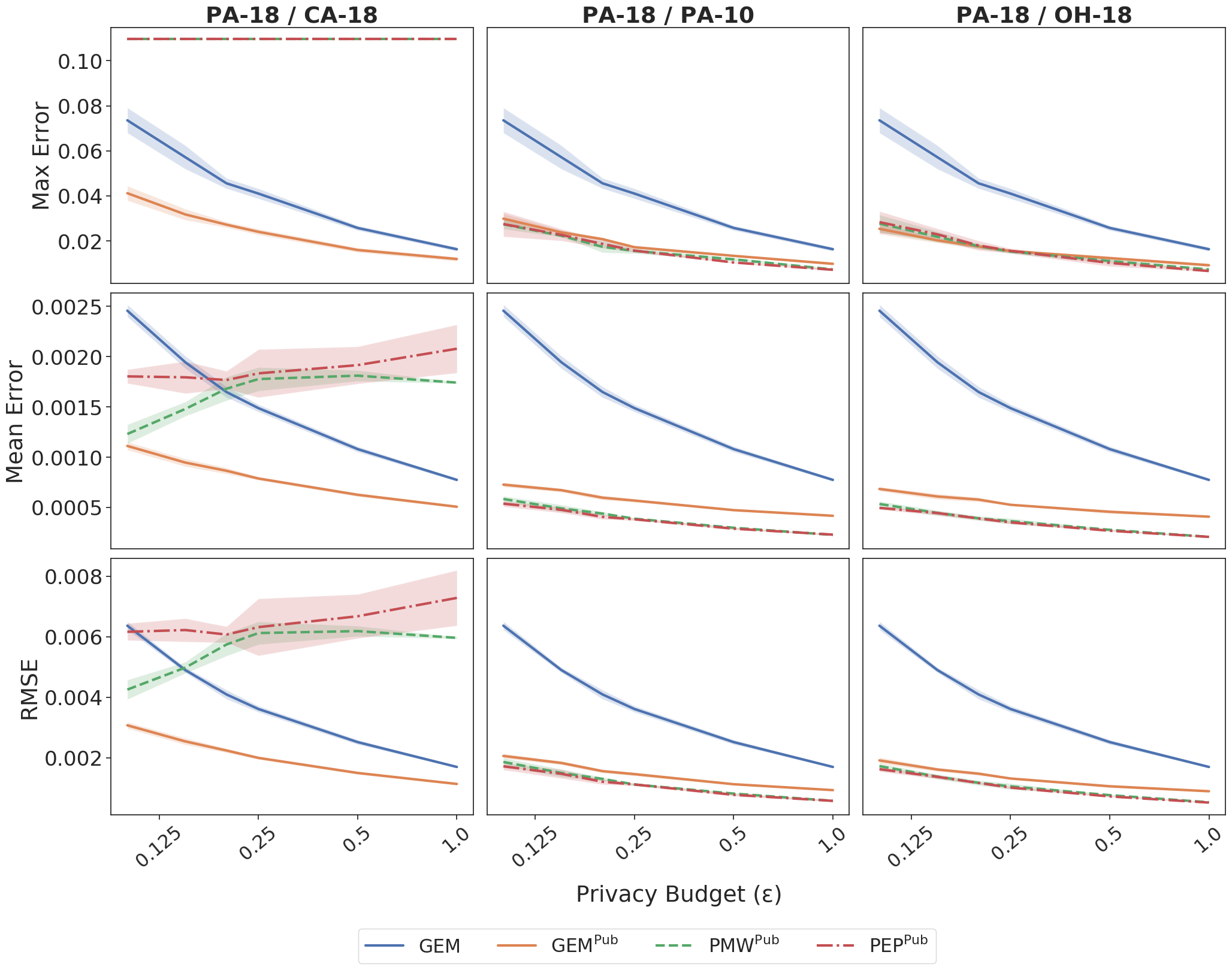
Figure 6: Max, mean, and mean squared error for $3$-way marginals on ACS PA-18 (workloads = $4096$) with privacy budgets $\varepsilon\in\{0.1,0.15,0.2,0.25,0.5,1\}$ and $\delta=\frac{1}{n^{2}}$. We evaluate public-data-assisted algorithms with the following public datasets: Left: 2018 California (CA-18); Center: 2010 Pennsylvania (PA-10); Right: 2018 Ohio (PA-10). The x-axis uses a logarithmic scale. Results are averaged over $5$ runs, and error bars represent one standard error.

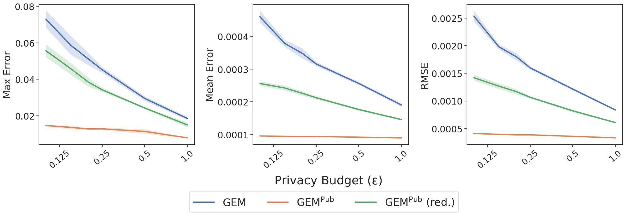
Figure 7: Max, mean, and mean squared error for $3$-way marginals on ADULT (workloads = $286$) with privacy budgets $\varepsilon\in\{0.1,0.15,0.2,0.25,0.5,1\}$ and $\delta=\frac{1}{n^{2}}$. We evaluate GEM using both the complete public data (GEM^Pub) and a reduced version that has fewer attributes (GEM^Pub (reduced)). The x-axis uses a logarithmic scale. Results are averaged over $5$ runs, and error bars represent one standard error.

In Figures 5, 6, and 7, we present the same results for the same experiments described in Section 7.1 (Figures 1 and 2), adding plots for mean error and root mean squared error (RMSE). For our experiments on ACS PA-18 with public data, we add results using 2018 data for Ohio (ACS OH-18), which we note also low best-mixture-error. Generally, the relative performance between the methods for these other two metrics is the same as for max error.

In addition, in Figure 6, we present results for PEP^Pub, a version of PEP similar to PMW^Pub that is adapted to leverage public data (and consequently can be applied to high dimensional settings). We briefly describe the details below.

PEP^Pub. Like in liu2021leveraging, we extend PEP by making two changes: (1) we maintain a distribution over the public data domain and (2) we initialize the approximating distribution to that of the public dataset. Therefore like PMW^Pub, PEP^Pub also restricts $\mathcal{D}$ to distributions over the public data domain and initializes $D_{0}$ to be the public data distribution.

We note that PEP^Pub performs similarly to PMW^Pub, making it unable to perform well when using ACS CA-18 as a public dataset (for experiments on ACS PA-18). Similarly, it cannot be feasibly run for the ADULT dataset when the public dataset is missing a significant number of attributes.

D.3 Comparisons against RAP

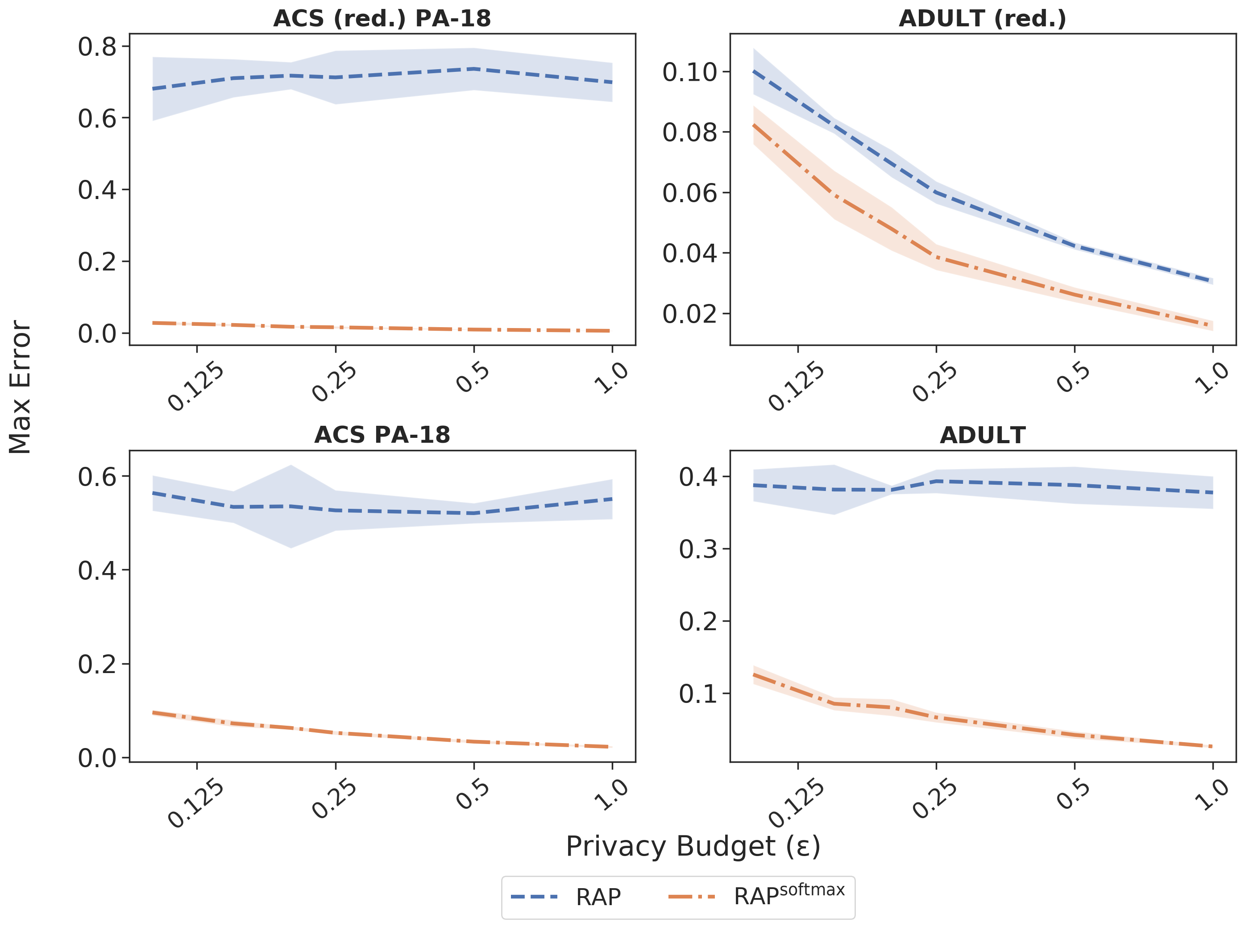
Figure 8: Comparison of RAP and RAP^softmax w.r.t max error for $3$-way marginals evaluated on ADULT and ACS PA-18 using privacy budgets $\varepsilon\in\{0.1,0.15,0.2,0.25,0.5,1\}$ and $\delta=\frac{1}{n^{2}}$. The x-axis uses a logarithmic scale. We evaluate using the following workload sizes: ACS (reduced) PA-18: $455$; ACS PA-18: $4096$; ADULT (reduced): $286$; ADULT: $35$. Results are averaged over $5$ runs, and error bars represent one standard error.

In Figure 8, we show failures cases for RAP. Again, we see that RAP^softmax outperforms RAP in every setting. However, we observe that aside from ADULT (reduced), RAP performs extremely poorly across all privacy budgets.

To account for this observation, we hypothesize that by projecting each measurement to aydore2021differentially’s proposed continuous relaxation of the synthetic dataset domain, RAP produces a synthetic dataset that is inconsistent with the semantics of an actual dataset. Such inconsistencies make it more difficult for the algorithm to do well without seeing the majority of high error queries.

Consider this simple example comparing GEM and RAP. Suppose we have some binary attribute $A\in\left\{0,1\right\}$ and we have $P(A=0)=0.2$ and $P(A=1)=0.8$. For simplicity, suppose that the initial answers at $t=0$ for both algorithms is $0$ for the queries $q_{A=0}$ and $q_{A=1}$. Assume at $t=1$ that the privacy budget is large enough such that both algorithms select the max error query $q_{A=1}$ (error of $0.8$), which gives us an error or $0.8$. After a single iteration, both algorithms can reduce the error of this query to $0$. In RAP, the max error then is $0.2$ (for the next largest error query $q_{A=0}$). However for GEM to output the correct answer for $q_{A=1}$, it must learn a distribution (due to the softmax activation function) such that $P(A=1)=0.8$, which naturally forces $P(A=0)=0.2$. In this way, GEM can reduce the errors of both queries in one step, giving it an advantage over RAP.

In general, algorithms within the Adaptive Measurements framework have this advantage in that the answers it provides must be consistent with the data domain. For example, if again we consider the two queries for attribute $A$, a simple method like the Gaussian or Laplace mechanism has a nonzero probability of outputting noisy answers for $q_{A=0}$ and $q_{A=1}$ such that $P(A=0)+P(A=1)\neq 1$. This outcome however will never occur in Adaptive Measurements.

Therefore, we hypothesize that RAP tends to do poorly as you increase the number of high error queries because the algorithm needs to select each high error query to obtain low error. Synthetic data generation algorithms can more efficiently make use of selected query measurements because their answers to all possible queries must be consistent. Referring to the above example again, there may exist two high error queries $q_{A=0}$ and $q_{A=1}$, but only one needs to be sampled to reduce the errors of both.

We refer readers to Appendix D.7, where we use the above discussion to account for how the way in which the continuous attributes in ADULT are preprocessed can impact the effectiveness of RAP.

D.4 Marginal trick

While this work follows the literature in which methods iteratively sample sensitivity $1$ queries, we note that the marginal trick approach (Appendix A.1) can be applied to all iterative algorithms under Adaptive Measurements. To demonstrate this marginal trick’s effectiveness, we show in Figure 9 how the performance of GEM improves across max, mean, and root mean squared error by replacing the Update and Measure steps in Adaptive Measurements.

In this experiment, given that the number of measurements taken is far greater when using the marginal trick, we increased $T_{max}$ for GEM from $100$ to $10000$ and changed the loss function from $\ell_{1}$-loss to $\ell_{2}$-loss. Additional hyperparameters used can be found in Table 6. Note that we reduced the model size for $G$ simply to speed up runtime. Overall, we admit that leveraging this trick was not our focus, and so we leave designing GEM (and other iterative methods) to fully take advantage of the marginal trick to future work.

Table 6: GEM (marginal trick) hyperparameters

Dataset	Parameter	Values
All	hidden layer sizes	$(256,512)$
	learning rate	$0.0001$
	$B$	$1000$
	$\alpha$	$0.5$
	$T_{max}$	$10000$
ACS	$T$	$50$, $100$, $150$, $200$,
		$250$, $300$, $400$, $500$
ACS (red.)	$T$	$50$, $100$, $150$, $200$,
		$250$, $300$, $450$
ADULT	$T$	$30$, $40$, $50$, $75$,
		$100$, $125$, $150$, $200$
ADULT (red.)	$T$	$5$, $10$, $15$, $20$
		$25$, $30$, $35$

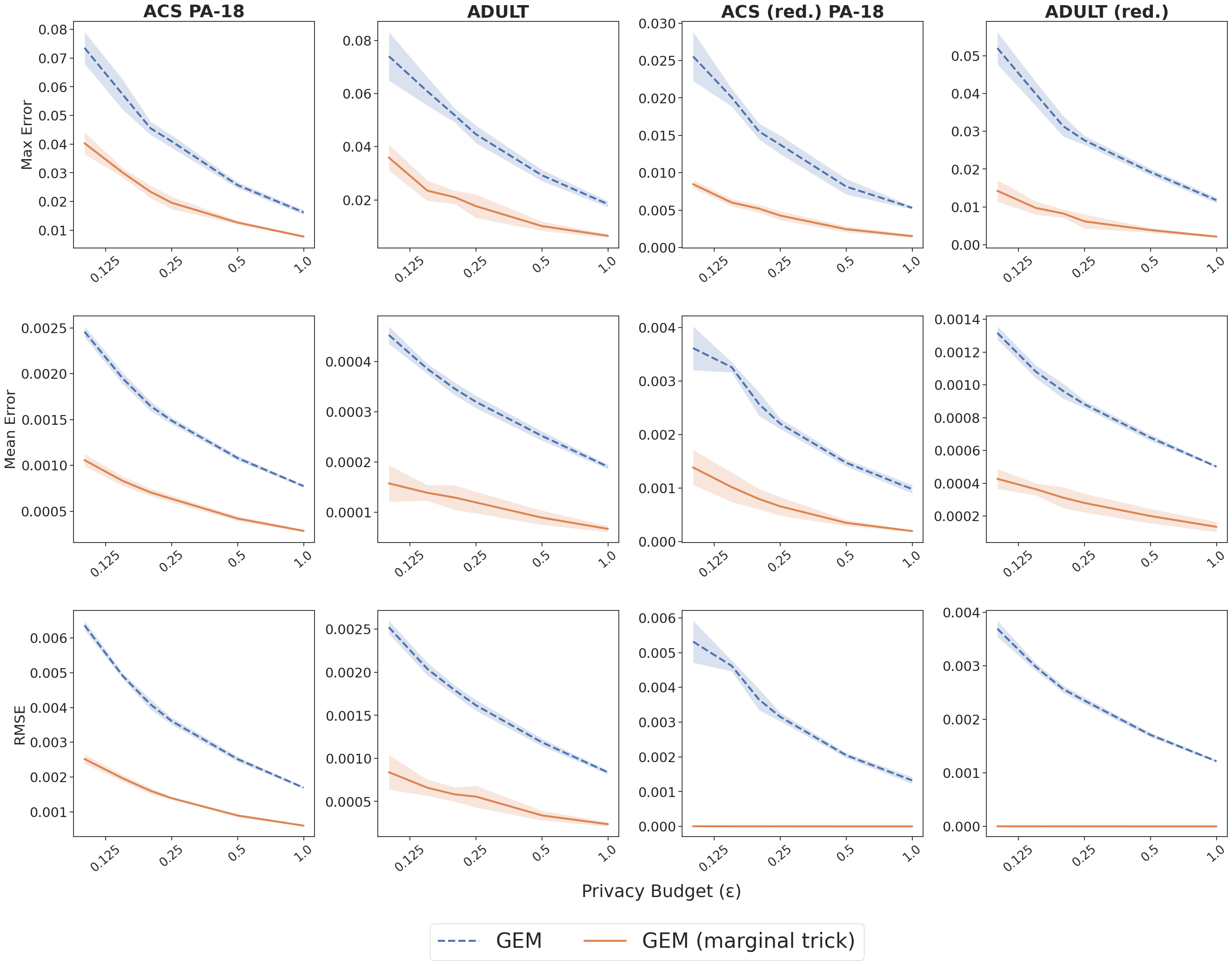
Figure 9: Error comparison of GEM with and without the marginal trick , evaluated on $3$-way marginals with privacy budgets $\varepsilon\in\{0.1,0.15,0.2,0.25,0.5,1\}$ and $\delta=\frac{1}{n^{2}}$. The x-axis uses a logarithmic scale. Results are averaged over $5$ runs, and error bars represent one standard error.

D.5 Discussion of HDMM

HDMM [mckenna2018optimizing] is an algorithm designed to directly answer a set of workloads, rather than some arbitrary set of queries. In particular, HDMM optimizes some strategy matrix to represent each workload of queries that in theory, facilitates an accurate reconstruction of the workload answers while decreasing the sensitivity of the privacy mechanisms itself. In their experiments, mckenna2018optimizing show strong results w.r.t. RMSE, and the U.S. Census Bureau itself has incorporated aspects of the algorithm into its own releases [Kifer19].

We originally planned to run HDMM as a baseline for our algorithms in the standard setting, but after discussing with the original authors, we learned that currently, the available code for HDMM makes running the algorithm difficult for the ACS and ADULT datasets. There is no way to solve the least square problem described in the paper for domain sizes larger than $10^{9}$, and while the authors admit that HDMM could possibly be modified to use local least squares for general workloads (outside of those defined in their codebase), this work is not expected to be completed in the near future.

We also considered running HDMM+PGM [mckenna2019graphical], which replaces the least squares estimation problem a graphical model estimation algorithm. Specifically, using (differentially private) measurements to some set of input queries, HDMM+PGM infers answers for any workload of queries. However, the memory requirements of the algorithm scale exponentially with dimension of the maximal clique of the measurements, prompting users to carefully select measurements that help build a useful junction tree that is not too dense. Therefore, the choice of measurements and cliques can be seen as hyperparameters for HDMM+PGM, but as the authors pointed out to us, how such measurements should be selected is an open problem that hasn’t been solved yet. In general, cliques should be selected to capture correlated attributes without making the size of the graphical model intractable. However, we were unsuccessful in finding a set of measurements that achieved sensible results (possibly due to the large number of workloads our experiments are designed to answer) and decided stop pursuing this endeavor due to the heavy computational resources required to run HDMM+PGM. We leave finding a proper set of measurements for ADULT and ACS PA-18 as an open problem.

Given such limitations, we evaluate HDMM with least squares on ACS (reduced) PA-18 and ADULT (reduced) only (Figure 10). We use the implementation found in https://github.com/ryan112358/private-pgm. We compare to GEM using the marginal trick, which HDMM also utilizes by default. While GEM outperforms HDMM, HDMM seems to be very competitive on low dimensional datasets when the privacy budget is higher. In particular, HDMM slightly outperforms GEM w.r.t. max error on ACS (reduced) when $\varepsilon=1$. We leave further investigation of HDMM and HDMM+PGM to future work.

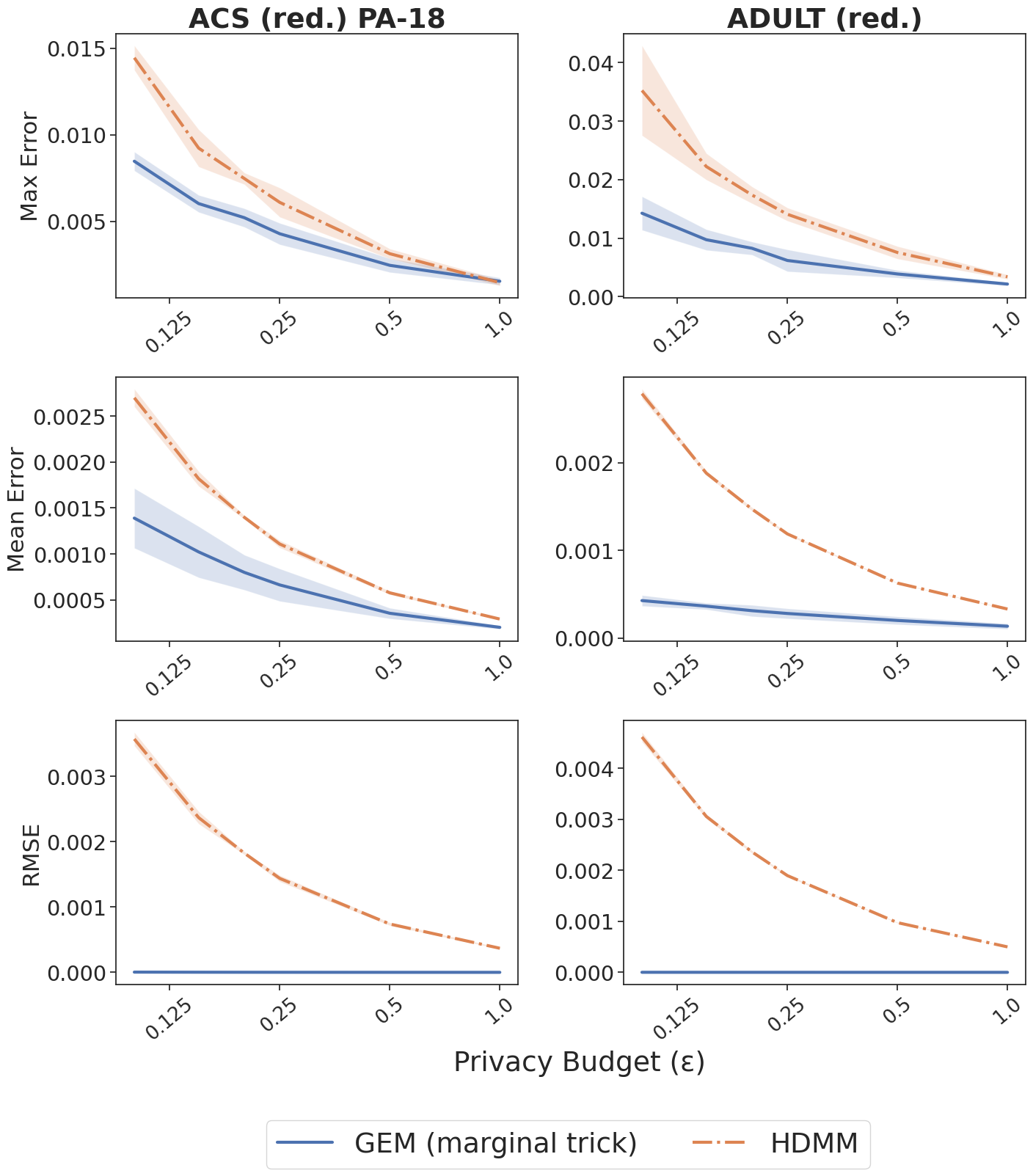
Figure 10: Comparison of max, mean, and root mean squared errors against HDMM on ACS (reduced) PA-18 (workloads=455) and ADULT (reduced) (workloads=35), evaluated on $3$-way marginals with privacy budgets $\varepsilon\in\{0.1,0.15,0.2,0.25,0.5,1\}$ and $\delta=\frac{1}{n^{2}}$. The x-axis uses a logarithmic scale. Results are averaged over $5$ runs, and error bars represent one standard error.

D.6 Effectiveness of optimizing over past queries

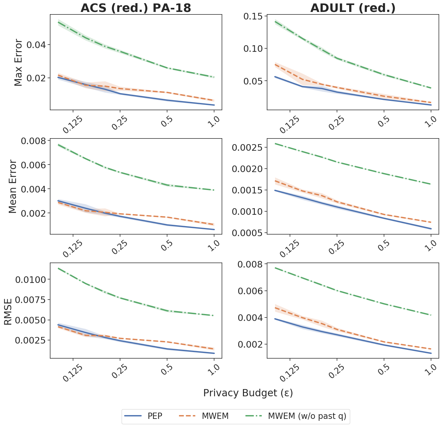
Figure 11: Comparison of max, mean, and root mean squared errors against vanilla MWEM that does not use queries sampled during past iterations, evaluated on $3$-way marginals with privacy budgets $\varepsilon\in\{0.1,0.15,0.2,0.25,0.5,1\}$ and $\delta=\frac{1}{n^{2}}$. The x-axis uses a logarithmic scale. Results are averaged over $5$ runs, and error bars represent one standard error.

One important part of the adaptive framework is that it encompasses algorithms whose update step uses measurements from past iterations. In Figure 11, we verify claims from hardt2010simple and liu2021leveraging that empirically, we can significantly improve over the performance of MWEM when incorporating past measurements.

D.7 Evaluating on ADULT* and LOANS

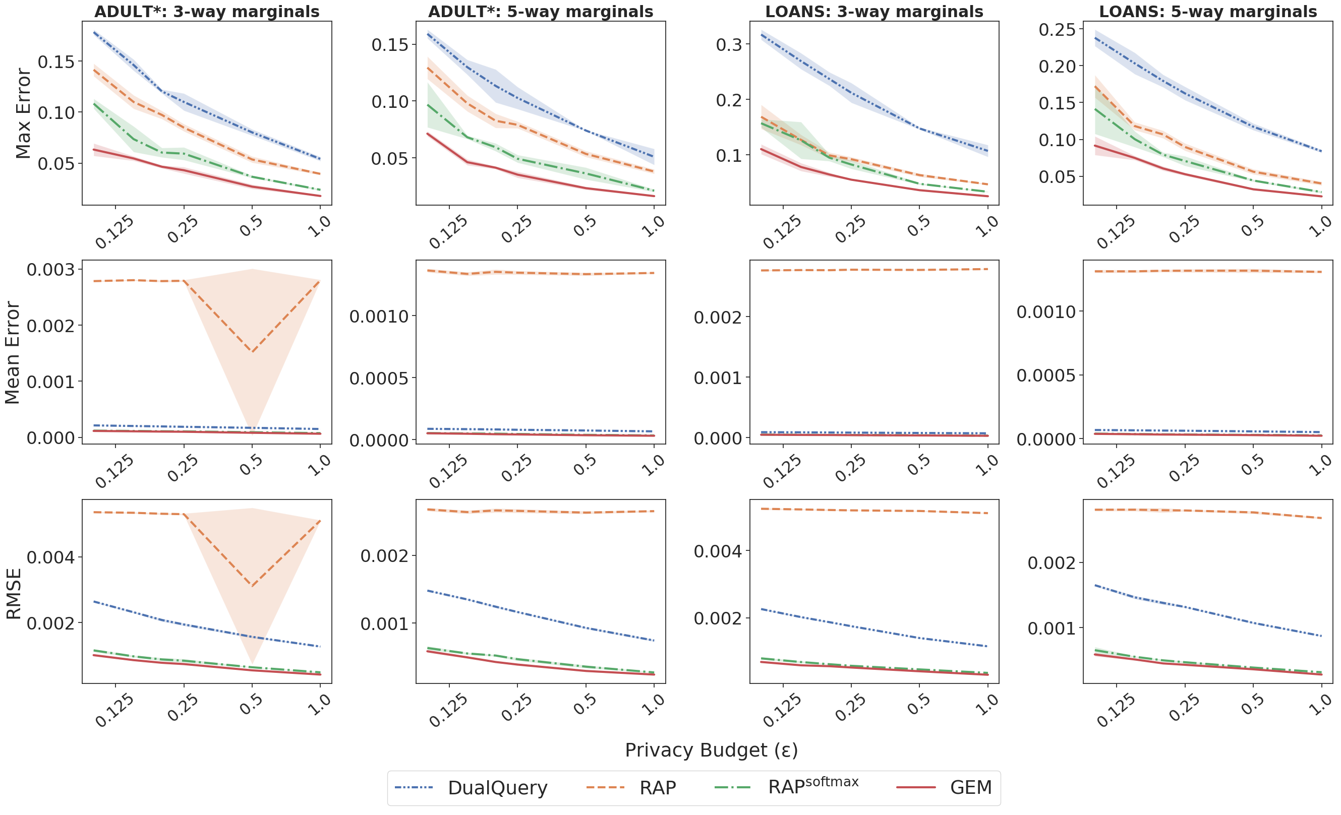
Figure 12: Max, mean, and root mean squared errors for $3$-way marginals with a workload size of $64$. Methods are evaluated on ADULT* and LOANS datasets using privacy budgets $\varepsilon\in\{0.1,0.15,0.2,0.25,0.5,1\}$ and $\delta=\frac{1}{n^{2}}$. The x-axis uses a logarithmic scale. Results are averaged over $5$ runs, and error bars represent one standard error.

In Figure 12, we reproduce the experiments on the ADULT (which we denote as ADULT*) and LOANS datasets presented in aydore2021differentially. Like aydore2021differentially, we obtain the datasets from https://github.com/giusevtr/fem. Empirically, we find that GEM outperforms all baseline methods. In addition, while RAP performs reasonably well, we observe that by confining $\mathcal{D}$ to $\left\{\sigma(M)|M\in\mathbb{R}^{n^{\prime}\times d}\right\}$ with the softmax function, RAP^softmax performs better across all privacy budgets.

To account for why RAP performs reasonably well with respect to max error on ADULT* and LOANs but very poorly on ADULT and ACS, we refer back to our discussion about the issues of RAP presented in Appendix D.3 in which argue that by outputting synthetic data that is inconsistent with any real dataset, RAP performs poorly when there are many higher error queries. ADULT* and LOANs are preprocessed in a way such that continous attributes are converted into categorical (technically ordinal) attributes, where a separate categorical value is created for each unique value that the continuous attribute takes on in the dataset (up to a maximum of $100$ unique values). When processed in this way, $k$-way marginal query answers are sparser, even when $k$ is relatively small ($\leq 5$). However, liu2021leveraging preprocess continuous variables in the ADULT and ACS dataset by constructing bins, resulting in higher error queries.

For example, suppose in an unprocessed dataset (with $n$ rows), you have $3$ rows where an attribute (such as income) takes on the values $16,587$, $15,984$, and $18,200$. Next, suppose there exists datasets A and B, where dataset A maps each unique value to its own category, while dataset B constructs a bin for values between $15,000$ and $20,000$. Then considering all $1$-way marginal queries involving this attribute, dataset A would have $3$ different queries, each with answer $\frac{1}{N}$. Dataset B however would only have a single query whose answer is $\frac{3}{N}$. Whether a dataset should be preprocessed as dataset A or dataset B depends on the problem setting. However, this (somewhat contrived) example demonstrates how dataset B would have more queries with high value answers (and therefore more queries with high initial errors, assuming that the algorithms in question initially outputs answers that are uniform/close to $0$).

In our experiments with $3$-way marginal queries, ADULT (where workload is $286$) and ADULT* (where the workload is $64$) have roughly the same number queries ($334,128$ vs. $458,996$ respectively). However, ADULT has $487$ queries with answers above $0.1$ while ADULT* only has $71$. Looking up the number of queries with answers above $0.2$, we count $181$ for ADULT and only $28$ for ADULT*. Therefore, experiments on ADULT* have fewer queries that RAP needs to optimize over to achieve low max error, which we argue accounts for the differences in performance on the two datasets.

Finally, we note that in Figure 8, RAP has relatively high mean error and RMSE. We hypothesize that again, because only the queries selected on each round are optimized and all other query answers need not be consistent with the optimized ones, RAP will not perform well on any metric that is evaluated over all queries (since due to privacy budget constraints, most queries/measurements are never seen by the algorithm). We leave further investigation on how RAP operates in different settings to future work.

References

- Abadi et al. [2015] Martín Abadi, Ashish Agarwal, Paul Barham, Eugene Brevdo, Zhifeng Chen, Craig Citro, Greg S. Corrado, Andy Davis, Jeffrey Dean, Matthieu Devin, Sanjay Ghemawat, Ian Goodfellow, Andrew Harp, Geoffrey Irving, Michael Isard, Yangqing Jia, Rafal Jozefowicz, Lukasz Kaiser, Manjunath Kudlur, Josh Levenberg, Dandelion Mané, Rajat Monga, Sherry Moore, Derek Murray, Chris Olah, Mike Schuster, Jonathon Shlens, Benoit Steiner, Ilya Sutskever, Kunal Talwar, Paul Tucker, Vincent Vanhoucke, Vijay Vasudevan, Fernanda Viégas, Oriol Vinyals, Pete Warden, Martin Wattenberg, Martin Wicke, Yuan Yu, and Xiaoqiang Zheng. TensorFlow: Large-scale machine learning on heterogeneous systems, 2015. URL https://www.tensorflow.org/. Software available from tensorflow.org.
- Abowd [2018] John M. Abowd. The U.S. census bureau adopts differential privacy. In ACM International Conference on Knowledge Discovery & Data Mining, page 2867, 2018.
- Alon et al. [2019] Noga Alon, Raef Bassily, and Shay Moran. Limits of private learning with access to public data. In H. Wallach, H. Larochelle, A. Beygelzimer, F. d'Alché-Buc, E. Fox, and R. Garnett, editors, Advances in Neural Information Processing Systems, volume 32. Curran Associates, Inc., 2019. URL https://proceedings.neurips.cc/paper/2019/file/9a6a1aaafe73c572b7374828b03a1881-Paper.pdf.
- Aydore et al. [2021] Sergul Aydore, William Brown, Michael Kearns, Krishnaram Kenthapadi, Luca Melis, Aaron Roth, and Ankit Siva. Differentially private query release through adaptive projection. arXiv preprint arXiv:2103.06641, 2021.
- Bassily et al. [2020a] Raef Bassily, Albert Cheu, Shay Moran, Aleksandar Nikolov, Jonathan R. Ullman, and Zhiwei Steven Wu. Private query release assisted by public data. In Proceedings of the 37th International Conference on Machine Learning, ICML 2020, 13-18 July 2020, Virtual Event, volume 119 of Proceedings of Machine Learning Research, pages 695–703. PMLR, 2020a. URL http://proceedings.mlr.press/v119/bassily20a.html.
- Bassily et al. [2020b] Raef Bassily, Shay Moran, and Anupama Nandi. Learning from mixtures of private and public populations. In Hugo Larochelle, Marc’Aurelio Ranzato, Raia Hadsell, Maria-Florina Balcan, and Hsuan-Tien Lin, editors, Advances in Neural Information Processing Systems 33: Annual Conference on Neural Information Processing Systems 2020, NeurIPS 2020, December 6-12, 2020, virtual, 2020b. URL https://proceedings.neurips.cc/paper/2020/hash/1ee942c6b182d0f041a2312947385b23-Abstract.html.
- Beaulieu-Jones et al. [2019] Brett K Beaulieu-Jones, Zhiwei Steven Wu, Chris Williams, Ran Lee, Sanjeev P Bhavnani, James Brian Byrd, and Casey S Greene. Privacy-preserving generative deep neural networks support clinical data sharing. Circulation: Cardiovascular Quality and Outcomes, 12(7):e005122, 2019.
- Blum et al. [2008] Avrim Blum, Katrina Ligett, and Aaron Roth. A learning theory approach to non-interactive database privacy. In Cynthia Dwork, editor, Proceedings of the 40th Annual ACM Symposium on Theory of Computing, Victoria, British Columbia, Canada, May 17-20, 2008, pages 609–618. ACM, 2008. doi: 10.1145/1374376.1374464. URL https://doi.org/10.1145/1374376.1374464.
- Bun and Steinke [2016] Mark Bun and Thomas Steinke. Concentrated differential privacy: Simplifications, extensions, and lower bounds. In Proceedings of the 14th Conference on Theory of Cryptography, TCC ’16-B, pages 635–658, Berlin, Heidelberg, 2016. Springer.
- Bun et al. [2018] Mark Bun, Jonathan Ullman, and Salil Vadhan. Fingerprinting codes and the price of approximate differential privacy. SIAM Journal on Computing, 47(5):1888–1938, 2018.
- Cesar and Rogers [2020] Mark Cesar and Ryan Rogers. Unifying privacy loss composition for data analytics. arXiv preprint arXiv:2004.07223, 2020.
- Dua and Graff [2017] Dheeru Dua and Casey Graff. UCI machine learning repository, 2017. URL http://archive.ics.uci.edu/ml.
- Dwork and Rothblum [2016] Cynthia Dwork and Guy N. Rothblum. Concentrated differential privacy, 2016.
- Dwork et al. [2006] Cynthia Dwork, Frank McSherry, Kobbi Nissim, and Adam Smith. Calibrating noise to sensitivity in private data analysis. In Proceedings of the 3rd Conference on Theory of Cryptography, TCC ’06, pages 265–284, Berlin, Heidelberg, 2006. Springer.
- Dwork et al. [2009] Cynthia Dwork, Moni Naor, Omer Reingold, Guy N. Rothblum, and Salil Vadhan. On the complexity of differentially private data release: Efficient algorithms and hardness results. In Proceedings of the Forty-First Annual ACM Symposium on Theory of Computing, STOC ’09, page 381–390, New York, NY, USA, 2009. Association for Computing Machinery. ISBN 9781605585062. doi: 10.1145/1536414.1536467. URL https://doi.org/10.1145/1536414.1536467.
- Edmonds et al. [2020] Alexander Edmonds, Aleksandar Nikolov, and Jonathan Ullman. The power of factorization mechanisms in local and central differential privacy. In Proceedings of the 52nd Annual ACM SIGACT Symposium on Theory of Computing, STOC 2020, page 425–438, New York, NY, USA, 2020. Association for Computing Machinery. ISBN 9781450369794. doi: 10.1145/3357713.3384297. URL https://doi.org/10.1145/3357713.3384297.
- Gaboardi et al. [2014] Marco Gaboardi, Emilio Jesús Gallego Arias, Justin Hsu, Aaron Roth, and Zhiwei Steven Wu. Dual query: Practical private query release for high dimensional data. In International Conference on Machine Learning, pages 1170–1178. PMLR, 2014.
- Gupta et al. [2012] Anupam Gupta, Aaron Roth, and Jonathan Ullman. Iterative constructions and private data release. In Proceedings of the 9th International Conference on Theory of Cryptography, TCC’12, page 339–356, Berlin, Heidelberg, 2012. Springer-Verlag. ISBN 9783642289132. doi: 10.1007/978-3-642-28914-9_19. URL https://doi.org/10.1007/978-3-642-28914-9_19.
- Hardt and Rothblum [2010] Moritz Hardt and Guy N Rothblum. A multiplicative weights mechanism for privacy-preserving data analysis. In 2010 IEEE 51st Annual Symposium on Foundations of Computer Science, pages 61–70. IEEE, 2010.
- Hardt et al. [2012] Moritz Hardt, Katrina Ligett, and Frank Mcsherry. A simple and practical algorithm for differentially private data release. In F. Pereira, C. J. C. Burges, L. Bottou, and K. Q. Weinberger, editors, Advances in Neural Information Processing Systems, volume 25. Curran Associates, Inc., 2012. URL https://proceedings.neurips.cc/paper/2012/file/208e43f0e45c4c78cafadb83d2888cb6-Paper.pdf.
- Kifer [2019] Daniel Kifer. Consistency with external knowledge: The topdown algorithm, 2019. http://www.cse.psu.edu/~duk17/papers/topdown.pdf.
- Li et al. [2015] Chao Li, Gerome Miklau, Michael Hay, Andrew Mcgregor, and Vibhor Rastogi. The matrix mechanism: Optimizing linear counting queries under differential privacy. The VLDB Journal, 24(6):757–781, December 2015. ISSN 1066-8888. doi: 10.1007/s00778-015-0398-x. URL https://doi.org/10.1007/s00778-015-0398-x.
- Liu et al. [2021] Terrance Liu, Giuseppe Vietri, Thomas Steinke, Jonathan Ullman, and Zhiwei Steven Wu. Leveraging public data for practical private query release. arXiv preprint arXiv:2102.08598, 2021.
- Martins and Astudillo [2016] Andre Martins and Ramon Astudillo. From softmax to sparsemax: A sparse model of attention and multi-label classification. In International conference on machine learning, pages 1614–1623. PMLR, 2016.
- McKenna et al. [2018] Ryan McKenna, Gerome Miklau, Michael Hay, and Ashwin Machanavajjhala. Optimizing error of high-dimensional statistical queries under differential privacy. Proc. VLDB Endow., 11(10):1206–1219, June 2018. ISSN 2150-8097. doi: 10.14778/3231751.3231769. URL https://doi.org/10.14778/3231751.3231769.
- McKenna et al. [2019] Ryan McKenna, Daniel Sheldon, and Gerome Miklau. Graphical-model based estimation and inference for differential privacy. In International Conference on Machine Learning, pages 4435–4444. PMLR, 2019.
- Neunhoeffer et al. [2021] Marcel Neunhoeffer, Steven Wu, and Cynthia Dwork. Private post-{gan} boosting. In International Conference on Learning Representations, 2021. URL https://openreview.net/forum?id=6isfR3JCbi.
- Nikolov et al. [2013] Aleksandar Nikolov, Kunal Talwar, and Li Zhang. The geometry of differential privacy: The sparse and approximate cases. In Proceedings of the Forty-Fifth Annual ACM Symposium on Theory of Computing, STOC ’13, page 351–360, New York, NY, USA, 2013. Association for Computing Machinery. ISBN 9781450320290. doi: 10.1145/2488608.2488652. URL https://doi.org/10.1145/2488608.2488652.
- Paszke et al. [2019] Adam Paszke, Sam Gross, Francisco Massa, Adam Lerer, James Bradbury, Gregory Chanan, Trevor Killeen, Zeming Lin, Natalia Gimelshein, Luca Antiga, Alban Desmaison, Andreas Kopf, Edward Yang, Zachary DeVito, Martin Raison, Alykhan Tejani, Sasank Chilamkurthy, Benoit Steiner, Lu Fang, Junjie Bai, and Soumith Chintala. Pytorch: An imperative style, high-performance deep learning library. In H. Wallach, H. Larochelle, A. Beygelzimer, F. d'Alché-Buc, E. Fox, and R. Garnett, editors, Advances in Neural Information Processing Systems 32, pages 8024–8035. Curran Associates, Inc., 2019. URL http://papers.neurips.cc/paper/9015-pytorch-an-imperative-style-high-performance-deep-learning-library.pdf.
- Roth and Roughgarden [2010] Aaron Roth and Tim Roughgarden. Interactive privacy via the median mechanism. In Leonard J. Schulman, editor, Proceedings of the 42nd ACM Symposium on Theory of Computing, STOC 2010, Cambridge, Massachusetts, USA, 5-8 June 2010, pages 765–774. ACM, 2010. doi: 10.1145/1806689.1806794. URL https://doi.org/10.1145/1806689.1806794.
- Ruggles et al. [2020] S Ruggles et al. Ipums usa: Version 10.0, doi: 10.18128/d010. V10. 0, 2020.
- Schapire and Freund [2013] Robert E Schapire and Yoav Freund. Boosting: Foundations and algorithms. Kybernetes, 2013.
- Ullman [2013] Jonathan Ullman. Answering n<sub>2+o(1)</sub> counting queries with differential privacy is hard. In Proceedings of the Forty-Fifth Annual ACM Symposium on Theory of Computing, STOC ’13, page 361–370, New York, NY, USA, 2013. Association for Computing Machinery. ISBN 9781450320290. doi: 10.1145/2488608.2488653. URL https://doi.org/10.1145/2488608.2488653.
- Ullman [2015] Jonathan Ullman. Private multiplicative weights beyond linear queries. In Proceedings of the 34th ACM SIGMOD-SIGACT-SIGAI Symposium on Principles of Database Systems, PODS ’15, page 303–312, New York, NY, USA, 2015. Association for Computing Machinery. ISBN 9781450327572. doi: 10.1145/2745754.2745755. URL https://doi.org/10.1145/2745754.2745755.
- Ullman and Vadhan [2011a] Jonathan Ullman and Salil Vadhan. Pcps and the hardness of generating private synthetic data. In Theory of Cryptography Conference, pages 400–416. Springer, 2011a.
- Ullman and Vadhan [2011b] Jonathan Ullman and Salil Vadhan. Pcps and the hardness of generating private synthetic data. In Yuval Ishai, editor, Theory of Cryptography, pages 400–416, Berlin, Heidelberg, 2011b. Springer Berlin Heidelberg. ISBN 978-3-642-19571-6.
- Vietri et al. [2020] Giuseppe Vietri, Grace Tian, Mark Bun, Thomas Steinke, and Steven Wu. New oracle-efficient algorithms for private synthetic data release. In International Conference on Machine Learning, pages 9765–9774. PMLR, 2020.
- Williams [1992] Ronald J Williams. Simple statistical gradient-following algorithms for connectionist reinforcement learning. Machine learning, 8(3):229–256, 1992.
- Xie et al. [2018] Liyang Xie, Kaixiang Lin, Shu Wang, Fei Wang, and Jiayu Zhou. Differentially private generative adversarial network. CoRR, abs/1802.06739, 2018. URL http://arxiv.org/abs/1802.06739.
- Yazıcı et al. [2018] Yasin Yazıcı, Chuan-Sheng Foo, Stefan Winkler, Kim-Hui Yap, Georgios Piliouras, and Vijay Chandrasekhar. The unusual effectiveness of averaging in gan training. arXiv preprint arXiv:1806.04498, 2018.
- Yoon et al. [2019] Jinsung Yoon, James Jordon, and Mihaela van der Schaar. PATE-GAN: Generating synthetic data with differential privacy guarantees. In International Conference on Learning Representations, 2019. URL https://openreview.net/forum?id=S1zk9iRqF7.