Extensions of the Kahn–Saks inequality
for posets of width two

Abstract.

The Kahn–Saks inequality is a classical result on the number of linear extensions of finite posets. We give a new proof of this inequality for posets of width two and both elements in the same chain using explicit injections of lattice paths. As a consequence we obtain a $q$-analogue, a multivariate generalization and an equality condition in this case. We also discuss the equality conditions of the Kahn–Saks inequality for general posets and prove several implications between conditions conjectured to be equivalent.

1. Introduction

1.1. Foreword

The study of linear extensions of finite posets is surprisingly rich as they generalize permutations, combinations, standard Young tableaux, etc. By contrast, the inequalities for the numbers of linear extensions are quite rare and difficult to prove as they have to hold for all posets. Posets of width two serve a useful middle ground as on the one hand there are sufficiently many of them to retain the diversity of posets, and on the other hand they can be analyzed by direct combinatorial tools.

In this paper, we study two classical results in the area: the Stanley inequality (1981), and its generalization, the Kahn–Saks inequality (1984). Both inequalities were proved using the geometric Alexandrov–Fenchel inequalities and remain largely mysterious. Despite much effort, no combinatorial proof of these inequalities has been found.

We give a new, fully combinatorial, proof of the Kahn–Saks inequality for posets of width two and both elements in the same chain. In this case, linear extensions are in bijection with certain lattice paths, and we prove the inequality by explicit injections. This is the approach first pioneered in [CFG80, GYY80] and more recently extended by the authors in [CPP21a]. In fact, Chung, Fishburn and Graham [CFG80] proved Stanley’s inequality for width two posets and their conjecture paved a way to Stanley’s paper [Sta81]. The details of our approach are somewhat different, but we do recover the Chung–Fishburn–Graham (CFG) injection as a special case. The construction in this paper is quite a bit more technical and is heavily based on ideas in our previous paper [CPP21a], where we established the cross-product conjecture in the special case of width two posets.

Now, our approach allows us to obtain $q$-analogues of both inequalities in the style of the $q$-cross-product inequality in [CPP21a]. More importantly, it is also robust enough to imply conditions for equality of the Kahn–Saks inequalities for the case of posets of width two and both elements in the same chain. The corresponding result for the Stanley inequality in the generality of all posets was obtained by Shenfeld and van Handel [SvH20+] using technology of geometric inequalities. Most recently, a completely different proof was obtained by the first two authors [CP21]. Although the equality condition in the special case of the Kahn–Saks inequality is the main result of paper, we start with a special case of the Stanley inequality as a stepping stone to our main results.

1.2. Two main inequalities

Let  $P=(X,\prec)$  be a finite poset. A linear extension of $P$ is a bijection  $L:X\to[n]$, such that  $L(x)<L(y)$  for all  $x\prec y$. Denote by  $\operatorname{\mathcal{E}}(P)$  the set of linear extensions of $P$, and write  $e(P):=|\operatorname{\mathcal{E}}(P)|$. The following are two key results in the area:

Theorem 1.1 (Stanley inequality [Sta81, Thm 3.1]).

Let  $P=(X,\prec)$  be a finite poset, and let  $x\in X$. Denote by  $\textrm{\em N}(k)$  the number of linear extensions  $L\in\operatorname{\mathcal{E}}(P)$, such that  $L(x)=k$. Then:

(1.1) $$\textrm{\em N}(k)^{2}\,\hskip 1.70709pt\geq\,\hskip 1.70709pt\textrm{\em N}(k-1)\,\hskip 1.70709pt\textrm{\em N}(k+1)\quad\text{for all}\quad k\hskip 1.70709pt>\hskip 1.70709pt1\hskip 0.85355pt.$$

In other words, the distribution of value of linear extensions on $x$ is log-concave.

Theorem 1.2 (Kahn–Saks inequality [KS84, Thm 2.5]).

Let  $x,y\in X$  be distinct elements of a finite poset  $P=(X,\prec)$. Denote by  $\textrm{\em F}(k)$  the number of linear extensions  $L\in\operatorname{\mathcal{E}}(P)$, such that  $L(y)-L(x)=k$. Then:

(1.2) $$\textrm{\em F}(k)^{2}\,\hskip 1.70709pt\geq\,\hskip 1.70709pt\textrm{\em F}(k-1)\,\hskip 1.70709pt\textrm{\em F}(k+1)\quad\text{for all}\quad k\hskip 1.70709pt>\hskip 1.70709pt1\hskip 0.85355pt.$$

Note that the Stanley inequality follows from the Kahn–Saks inequality by adding the maximal element $\hskip 0.85355pt\widehat{1}$  to the poset $P$, and letting  $y\leftarrow\widehat{1}$.

1.3. The $q$-analogues

From this point on, we consider only posets $P$ of width two. Fix a partition of $P$ into two chains  $\mathcal{C}_{1},\mathcal{C}_{2}\subset X$, where  $\mathcal{C}_{1}\cap\mathcal{C}_{2}=\varnothing$. Let  $\mathcal{C}_{1}=\{\alpha_{1},\ldots,\alpha_{\emph{{a}}}\}$  and  $\mathcal{C}_{2}=\{\beta_{1},\ldots,\beta_{\emph{{b}}}\}$  be these chains of lengths a and b, respectively. The weight of a linear extension $L\in\operatorname{\mathcal{E}}(P)$ is defined in [CPP21a] as

(1.3) $$\operatorname{\mathtt{wt}}(L)\ :=\ \sum_{i=1}^{\emph{{a}}}\,L(\alpha_{i})\hskip 1.70709pt.$$

Note that the definition of the weight  $\operatorname{\mathtt{wt}}(L)$  depends on the chain partition  $(\mathcal{C}_{1},\mathcal{C}_{2})$. We can now state our first two results.

Theorem 1.3 ($q$–Stanley inequality).

Let  $P=(X,\prec)$  be a finite poset of width two, let  $x\in X$, and let  $(\mathcal{C}_{1},\mathcal{C}_{2})$  be the chain partition as above. Define

$$\textrm{\em N}_{q}(k)\,:=\,\sum_{L\in\operatorname{\mathcal{E}}(P)\ :\ L(x)=k}\,q^{\operatorname{\mathtt{wt}}(L)}\hskip 1.70709pt.$$

Then:

(1.4) $$\textrm{\em N}_{q}(k)^{2}\ \geqslant\ \textrm{\em N}_{q}(k-1)\,\textrm{\em N}_{q}(k+1)\quad\ \text{ for all}\ \quad k\hskip 1.70709pt>\hskip 1.70709pt1\hskip 0.85355pt,$$

where the inequality between polynomials in  $q$  is coefficient-wise.

The following result is a generalization, sice we can always assume that element  $y=\widehat{1}$  is in the same chain as element $x$.

Theorem 1.4 ($q$–Kahn–Saks inequality).

Let  $x,y\in X$  be distinct elements of a finite poset  $P=(X,\prec)$  of width two. Suppose that either  $x,y\in\mathcal{C}_{1}$ , or  $x,y\in\mathcal{C}_{2}$. Define:

$$\textrm{\em F}_{q}(k)\ :=\ \sum_{L\in\operatorname{\mathcal{E}}(P)\ :\ L(y)-L(x)=k}\,q^{\operatorname{\mathtt{wt}}(L)}\hskip 1.70709pt.$$

Then:

(1.5) $$\textrm{\em F}_{q}(k)^{2}\,\geqslant\,\textrm{\em F}_{q}(k-1)\hskip 1.70709pt\textrm{\em F}_{q}(k+1)\quad\ \text{for all}\ \quad k\hskip 1.70709pt>\hskip 1.70709pt1\hskip 0.85355pt,$$

where the inequality between polynomials in  $q$  is coefficient-wise.

In Section 7, we give a multivariate generalization of both theorems. Note that the assumption that $x$ and $y$ belong to the same chain in the partition  $(\mathcal{C}_{1},\mathcal{C}_{2})$  are necessary for the conclusion of Theorem 1.4 to hold, as shown in the next example.

Example 1.5.

Let  $P=C_{3}+C_{3}$  be the disjoint sum of two chains with three elements. Denote these chains by  $\mathcal{C}_{1}:=\{\alpha_{1},\alpha_{2},\alpha_{3}\}$  and  $\mathcal{C}_{2}:=\{\beta_{1},\beta_{2},\beta_{3}\}$. For elements  $x=\alpha_{1}$  and  $y=\beta_{3}$, we have:

$$\textrm{F}_{q}(1)\,=\,q^{14}\hskip 1.70709pt,\quad\textrm{F}_{q}(2)\,=\,2\hskip 0.85355ptq^{13}\quad\text{and}\quad\textrm{F}_{q}(3)\,=\,3\hskip 0.85355ptq^{12}\hskip 1.70709pt+\hskip 1.70709ptq^{11}\hskip 0.85355pt.$$

We conclude:

$$\textrm{F}_{q}(2)^{2}\,-\,\textrm{F}_{q}(1)\,\textrm{F}_{q}(3)\ =\ q^{26}\hskip 1.70709pt-\hskip 1.70709ptq^{25}\ \not\geqslant\ 0\hskip 0.85355pt.$$

1.4. Equality conditions

Let $x=\alpha_{r}\in\mathcal{C}_{1}$. We say that $x$ satisfies a  $k$-pentagon property  if

$$\alpha_{r-1}\,\prec\,\beta_{k-r}\,\prec\,\beta_{k-r+1}\,\prec\,\alpha_{r+1}\qquad\text{and}\qquad\alpha_{r}\hskip 1.70709pt||\hskip 1.70709pt\beta_{k-r}\ \,,\ \ \alpha_{r}\hskip 1.70709pt||\hskip 1.70709pt\beta_{k-r+1}\ \,,$$

where  $u\hskip 1.70709pt||\hskip 1.70709ptv$  denotes incomparable elements  $u,v\in X$. In other words, the subposet of $P$ restricted to

$$\{\alpha_{r-1},\alpha_{r},\alpha_{r+1},\beta_{k-r},\beta_{k-r+1}\}$$

has a pentagonal Hasse diagram, see Figure 1.1. For  $x=\beta_{r}\in\mathcal{C}_{2}$  the $k$-pentagon property is defined analogously.

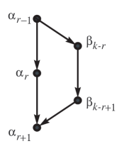
Figure 1.1. The $k$-pentagon property for  $x=\alpha_{r}\in\mathcal{C}_{1}$. The arrows point from smaller to larger elements in the poset.

Theorem 1.6 (Equality condition for the $q$-Stanley inequality, cf. Theorem 8.1).

Let  $P=(X,\prec)$  be a finite poset of width two. Fix  $x\in X$, and let  $\textrm{\em N}(k)$, $\textrm{\em N}_{q}(k)$  be defined as above. Suppose that  $k\in\{1,\ldots,n-1\}$  and  $\textrm{\em N}(k)>0$. Then the following are equivalent:

1. $\textrm{\em N}(k)^{2}\,=\,\textrm{\em N}(k-1)\,\textrm{\em N}(k+1)$,

2. $\textrm{\em N}(k)\,=\,\textrm{\em N}(k+1)\hskip 1.70709pt=\hskip 1.70709pt\textrm{\em N}(k-1)$,

3. $\textrm{\em N}_{q}(k)^{2}\,=\,\textrm{\em N}_{q}(k-1)\,\textrm{\em N}_{q}(k+1)$,

4. $\textrm{\em N}_{q}(k)\,=\,q^{\varepsilon}\hskip 0.85355pt\textrm{\em N}_{q}(k-1)\,=\,q^{-\varepsilon}\hskip 0.85355pt\textrm{\em N}_{q}(k+1)$,  where  $\varepsilon=1$  for  $x\in\mathcal{C}_{1}$  and  $\varepsilon=-1$  for  $x\in\mathcal{C}_{2}$ ,

5. element $x$ satisfies  $k$-pentagon property.

The equivalence  (a) $\Leftrightarrow$ (b) was recently proved by Shenfeld and van Handel [SvH20+] for general posets via a condition implying (e), see Theorem 8.1 and the discussion that follows. Conditions (c) and (d) are specific to posets of width two. The following result is a generalization of Theorem 1.6 and the main result of the paper:

Theorem 1.7 (Equality condition for the $q$-Kahn–Saks inequality).

Let  $x,y\in X$  be distinct elements of a finite poset  $P=(X,\prec)$  of width two. Let  $\textrm{\em F}(k)$, $\textrm{\em F}_{q}(k)$  be defined as above. Suppose that either $x,y\in\mathcal{C}_{1}$ or $x,y\in\mathcal{C}_{2}$. Also suppose that  $k\in\{2,\ldots,n-2\}$  and  $\textrm{\em F}(k)>0$. Then the following are equivalent:

1. $\textrm{\em F}(k)^{2}\,=\,\textrm{\em F}(k-1)\,\textrm{\em F}(k+1)$,

2. $\textrm{\em F}(k)\,=\,\textrm{\em F}(k+1)\,=\,\textrm{\em F}(k-1)$,

3. $\textrm{\em F}_{q}(k)^{2}\,=\,\textrm{\em F}_{q}(k-1)\,\textrm{\em F}_{q}(k+1)$,

4. $\textrm{\em F}_{q}(k)\,=q^{\varepsilon}\hskip 0.85355pt\textrm{\em F}_{q}(k-1)\,=\,q^{-\varepsilon}\hskip 0.85355pt\textrm{\em F}_{q}(k+1)$, for some  $\varepsilon\in\{\pm 1\}$,

5. there is an element  $z\in\{x,y\}$, such that for every  $L\in\operatorname{\mathcal{E}}(P)$  for which $L(y)-L(x)=k$,
   there are elements  $u,v\in X$  which satisfy  $u\hskip 1.70709pt||\hskip 1.70709ptz$,  $v\hskip 1.70709pt||\hskip 1.70709ptz$, and  $L(u)+1=L(z)=L(v)-1$.

Note that conditions (c) and (d) are specific to posets of width two. While conditions (a) and (b) do extend to general posets, the equivalence (a)  $\Leftrightarrow$  (b) does not hold in full generality. Even for the poset  $P=C_{3}+C_{3}$  of width two  given in Example 1.5, we have  $\textrm{F}(2)^{2}\hskip 1.70709pt=\hskip 1.70709pt\textrm{F}(3)\hskip 1.70709pt\textrm{F}(1)\hskip 1.70709pt=\hskip 1.70709pt4$,  even though  $\textrm{F}(1)=1$,  $\textrm{F}(2)=2$  and  $\textrm{F}(3)=4$.

We should also mention that the  $\textrm{F}(k)>0$  assumption is a very weak constraint, as the vanishing can be completely characterized for general posets (see Theorem 8.5). We refer to Section 8 for further discussion of general posets, and for the $k$-midway property which generalizes the $k$-pentagon property but is more involved.

1.5. Proof discussion

As we mentioned above, we start by translating the problem into a natural question about directed lattice paths in a row/column convex region in the grid (cf. $\S$9.4). From this point on, we do not work with posets and the proof becomes purely combinatorial enumeration of lattice paths.

While the geometric proofs in [KS84, Sta81] are quite powerful, the equality cases of the Alexandrov–Fenchel inequality are yet to be fully understood. So proving the equality conditions of poset inequalities is quite challenging, see [SvH20+, CP21] and $\S$9.1. This is why our direct combinatorial approach is so useful, as the explicit injection becomes a bijection in the case of equality.

In the case of Stanley’s inequality the CFG injection is quite simple and elegant, leading to a quick proof of the equality condition. For the Kahn–Saks inequality, the direct injection is a large composition of smaller injections, each of which is simple and either generalizes the CFG injection or of a different flavor, all influenced by the noncrossing paths in the Lindström–-Gessel–-Viennot lemma [GV89] (see also [GJ83, $\S$5.4]). Consequently, the equality condition of the Kahn–Saks inequality is substantially harder to obtain as one has to put together the equalities for each component of the proof and do a careful case analysis.

In summary, our proof of the main result (Theorem 1.7) is like an elaborate but delicious dish: the individual ingredients are elegant and natural, but the instruction on how they are put together is so involved the resulting recipe may seem difficult and unapproachable.

1.6. Structure of the paper

We start with an introductory Section 2 on posets, lattice paths, and lattice path inequalities. This section also includes some reformulated key lemmas from our previous paper [CPP21a], whose proof is sketched both for clarity and completeness. A reader very familiar with the standard definitions, notation and the results in [CPP21a] can safely skip this section.

In the next Section 3, we introduce key combinatorial lemmas which we employ throughout the paper: a criss–cross inequality (Lemma 3.1), and two equality lemmas (Lemma 3.2 and Lemma 3.3). In a short Section 4, we prove both the Stanley inequality (Theorem 1.1) which easily extends to the proof of the $q$-Stanley inequality (Theorem 1.3), and the equality conditions for Stanley’s inequality (Theorem 1.6). Even though these results are known in greater generality (except for Theorem 1.3 which is new), we recommend the reader not skip this section, as the proofs we present use the same approach as the following sections.

In Sections 5 and 6, we present the proofs of Theorems 1.4 and 1.7, respectively, by combining the previous tools together. These are the central sections of the paper. In a short Section 7, we give a multivariate generalizations of our $q$-analogues. Finally, in Section 8, we discuss generalizations of Theorem 1.7 to all finite posets. We state Conjecture 8.7 characterizing the complete equality conditionsi and prove several implications in support of the conjecture using the properties of promotion-like maps (see $\S$9.6). We conclude with final remarks and open problems in Section 9.

2. Lattice path inequalities

2.1. Basic notation

We use  $[n]=\{1,\ldots,n\}$,  $\mathbb{N}=\{0,1,2,\ldots\}$, and  $\mathbb{P}=\{1,2,\ldots\}$. Throughout the paper we use $q$ as a variable. For polynomials  $f,g\in\mathbb{Z}[q]$, we write  $f\leqslant g$  if the difference  $(g-f)\in\mathbb{N}[q]$, i.e. if  $(g-f)$  is a polynomial with nonnegative coefficients. Note the difference between relations

$$x\hskip 0.85355pt\preccurlyeq y\,,\quad a\hskip 0.85355pt\leq\hskip 0.85355ptb\,\quad\text{and}\quad f\leqslant\hskip 0.85355ptg\hskip 0.85355pt,$$

for posets elements, integers and polynomials, respectively.

2.2. Lattice path interpretation

Let $P=(X,\prec)$ be a finite poset of width two and let  $(\mathcal{C}_{1},\mathcal{C}_{2})$  be a fixed partition into two chains. Denote by  $\operatorname{\mathbf{0}}=(0,0)$  the origin and by  $\textbf{\hskip 0.85355pt{e}${}_{1}$}=(1,0)$,  $\textbf{\hskip 0.85355pt{e}${}_{2}$}=(0,1)$  two standard unit vectors in $\operatorname{\mathbb{Z}}^{2}$.

For a linear extension $L\in\operatorname{\mathcal{E}}(P)$, define the North–East (NE) lattice path  $\phi(L)$ obtained from $L$ by interpreting it as a sequence of North and East steps corresponding to elements in $\mathcal{C}_{1}$ and $\mathcal{C}_{2}$, respectively. Formally, let  $\phi(L):=(Z_{t})_{1\leq t\leq n}$  in  $\operatorname{\mathbb{Z}}^{2}$  from  $\operatorname{\mathbf{0}}=(0,0)$ to $(\emph{{a}},\emph{{b}})$, be the path  defined recursively as follows:

$$Z_{0}\,=\,\operatorname{\mathbf{0}},\qquad Z_{t}\ :=\ \begin{cases}\hskip 0.85355ptZ_{t-1}\hskip 0.85355pt+\hskip 0.85355pt\textbf{\hskip 0.85355pt{e}${}_{1}$}&\text{ if }\ L^{-1}(t)\in\mathcal{C}_{1}\hskip 1.70709pt,\\ \hskip 0.85355ptZ_{t-1}\hskip 0.85355pt+\hskip 0.85355pt\textbf{\hskip 0.85355pt{e}${}_{2}$}&\text{ if }\ L^{-1}(t)\in\mathcal{C}_{2}\hskip 1.70709pt.\end{cases}$$

Denote by $\operatorname{\textnormal{C}}(P)$ the set

$$\operatorname{\textnormal{C}_{\textnormal{up}}}(P)\ :=\ \bigg{\{}\left(h-\frac{1}{2},k-\frac{1}{2}\right)\in\operatorname{\mathbb{R}}^{2}\ :\ \alpha_{h}\hskip 1.70709pt\prec\hskip 1.70709pt\beta_{k}\,,\ 1\leq h\leq\emph{{a}},\ 1\leq k\leq\emph{{b}}\hskip 1.70709pt\bigg{\}}\hskip 1.70709pt,$$

$$\operatorname{\textnormal{C}_{\textnormal{down}}}(P)\ :=\ \bigg{\{}\left(h-\frac{1}{2},k-\frac{1}{2}\right)\in\operatorname{\mathbb{R}}^{2}\ :\ \alpha_{h}\hskip 1.70709pt\succ\hskip 1.70709pt\beta_{k}\,,\ 1\leq h\leq\emph{{a}},\ 1\leq k\leq\emph{{b}}\hskip 1.70709pt\bigg{\}}\hskip 1.70709pt.$$

Let $F_{\textnormal{up}}(P)$ and $F_{\textnormal{down}}(P)$ be the set of unit squares in $[0,\emph{{a}}]\times[0,\emph{{b}}]$ whose centers are in $\operatorname{\textnormal{C}_{\textnormal{up}}}(P)$ and $\operatorname{\textnormal{C}_{\textnormal{down}}}(P)$, respectively. Note that the region $F_{\textnormal{up}}(P)$ lies above the region $F_{\textnormal{down}}(P)$, and their interiors do not intersect. Let $\operatorname{\textnormal{Reg}}(P)$ be the (closed) region of $[0,\emph{{a}}]\times[0,\emph{{b}}]$ that is bounded from above by the region $F_{\textnormal{up}}(P)$, and from below by the region $F_{\textnormal{down}}(P)$, see Figure 2.1. It follows directly from the definition that $\operatorname{\textnormal{Reg}}(P)$ is a connected row and column convex region, with boundary defined by two lattice paths. Moreover, the lower boundary of $\operatorname{\textnormal{Reg}}(P)$ is the lattice path corresponding to the $\mathcal{C}_{1}$-minimal linear extension (i.e. assigning the smallest possible values to the elements of $\mathcal{C}_{1}$), and the upper boundary corresponds to the $\mathcal{C}_{1}$-maximal linear extension.

(a)	(b)

Figure 2.1. (a) The Hasse diagram of a poset $P$, and a linear extension $L$ of $P$ (written in red). (b) The corresponding region $\operatorname{\textnormal{Reg}}(P)$, with $F_{\textnormal{up}}(P)$ in green and $F_{\textnormal{down}}(P)$ in blue, and the lattice path $\phi(L)$ in red.

Lemma 2.1 ([CFG80, $\S$2] and [CPP21a, Lem 8.1]).

The map $\phi$ described above is a bijection between  $\operatorname{\mathcal{E}}(P)$  and NE lattice paths in  $\operatorname{\textnormal{Reg}}(P)$  from  $\operatorname{\mathbf{0}}$  to  $(\emph{{a}},\emph{{b}})$.

Remark 2.2.

It is not hard to see the regions  $\operatorname{\textnormal{Reg}}(P)$  which appear in Lemma 2.1 have no other constraints. Formally, for every region  $\Gamma\subset\mathbb{Z}^{2}$  between two noncrossing paths  $\gamma,\gamma^{\prime}:\hskip 0.85355pt\operatorname{\mathbf{0}}\to(\emph{{a}},\emph{{b}})$, there is a poset $P$ of width two with a partition into two chains of sizes  a and b, such that  $\Gamma=\operatorname{\textnormal{Reg}}(P)$. We leave the proof to the reader, see also $\S$9.4.

2.3. Inequalities for pairs of paths

We will use the lattice path inequalities from [CPP21a] and prove their extensions. In order to explain the combinatorics, we will briefly describe the proofs from [CPP21a]. Informally, they state that there are more pairs of paths which pass closer to the inside of the region than to the outside of the region.

Let  $A,B\in\operatorname{\textnormal{Reg}}(P)$. Denote by  $\mathcal{K}(A,B)$  the set of NE lattice paths  $\zeta:A\to B$, such that  $\zeta\in\operatorname{\textnormal{Reg}}(P)$. Similarly, denote by  $\textrm{K}_{q}(A,B)$  the polynomial

$$\textrm{K}_{q}(A,B)\ :=\ \sum_{\zeta\in\mathcal{K}(A,B)}\hskip 1.70709ptq^{\operatorname{\mathtt{wt}}(\zeta)}\,,$$

and we write  $\textrm{K}(A,B):=\textrm{K}_{1}(A,B)$  (i.e., when $q=1$).

Lemma 2.3 ([CPP21a, Lem 8.2]).

Let  $A,A^{\prime},B^{\prime},B\in\operatorname{\textnormal{Reg}}(P)$  be on the same vertical line with $A$ above $A^{\prime}$ such that $\overrightarrow{AA^{\prime}}=-\overrightarrow{BB^{\prime}}$ and $A^{\prime}$ on or above $B$, i.e.  $a_{1}=a_{1}^{\prime}=b_{1}=b_{1}^{\prime}$  and  $a_{2}-a_{2}^{\prime}=b_{2}^{\prime}-b_{2}$ with $a_{2}^{\prime}\geq b_{2}$. Let  $C,D\in\operatorname{\textnormal{Reg}}(P)$  be on a vertical line to the right of the line $AB$, and such that  $a^{\prime}_{2}-b_{2}\geq c_{2}-d_{2}$. Then:

$$\textrm{\em K}_{q}(A^{\prime},C)\,\cdot\,\textrm{\em K}_{q}(B^{\prime},D)\ \geqslant\ \textrm{\em K}_{q}(A,C)\,\cdot\,\textrm{\em K}_{q}(B,D).$$

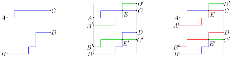
Figure 2.2. The proof of Lemma 2.3: The injection $\varkappa$ takes the blue paths $A\to C,B\to D$, translates the $B\to D$ path up to form the green path $A^{\prime}\to D^{\prime}$ (second picture), intersects it with the blue $A\to C$ path at $E$, and then forms the red path $A^{\prime}\to C$ (by following the green $A^{\prime}\to E$ and then switching to the blue $E\to C$. The other red path is obtained by translating the blue/green $A\to E\to D^{\prime}$ down.

Proof outline.

We exhibit an injection $\varkappa$ from pairs of paths  $\gamma:A\to C$,  $\delta:B\to D$  in  $\operatorname{\textnormal{Reg}}(P)$  to pairs of paths  $\gamma^{\prime}:A^{\prime}\to C$,  $\delta^{\prime}:B^{\prime}\to D$  in  $\operatorname{\textnormal{Reg}}(P)$. Let  $\operatorname{\mathbf{v}}=\overrightarrow{BA^{\prime}}$  and  $\widehat{\delta}=\delta+\operatorname{\mathbf{v}}$  be the translated path $\delta$, which starts at  $A^{\prime}=B+\operatorname{\mathbf{v}}$  and ends at  $D^{\prime}=D+\operatorname{\mathbf{v}}$, lying on or above $C$ by the condition in the Lemma. Then $\gamma$ and $\widehat{\delta}$ must intersect, and let $E$ be their first (closest to $A$) intersection point.

Now, let  $\gamma^{\prime}=\widehat{\delta}(A^{\prime},E)\circ\gamma(E,C)$, so  $\gamma^{\prime}:A^{\prime}\to C$. Similarly, let  $\delta^{\prime}=\gamma(A,E)\circ\widehat{\delta}(E,D^{\prime})\hskip 0.85355pt-\hskip 0.85355pt\operatorname{\mathbf{v}}$, so  $\delta^{\prime}:B^{\prime}\to D$. Then  $\gamma^{\prime}\subset\operatorname{\textnormal{Reg}}(P)$  since $\widehat{\delta}$ is on or above  $\delta\subset\operatorname{\textnormal{Reg}}(P)$ (because $a_{2}\geq b_{2}$) and is strictly below $\gamma\subset\operatorname{\textnormal{Reg}}(P)$ since $E$ is the first intersection point. Similarly, $\gamma(A,E)-\operatorname{\mathbf{v}}$  is also between $\gamma$ and $\delta$ and hence in $\operatorname{\textnormal{Reg}}(P)$. The other parts of  $\gamma^{\prime},\delta^{\prime}$  are part of the original paths $\gamma,\delta$ and so are also in $\operatorname{\textnormal{Reg}}(P)$. Then $\varkappa$ is clearly an injection. Since the paths are composed of the same pieces, some of which translated vertically with zero net effect, the total $q$-weight is preserved. ∎

3. Lattice paths toolkit expansion

3.1. Criss-cross inequalities

Here we consider inequalities between sums of pairs of paths.

Lemma 3.1 (Criss-cross lemma).

Let  $A,A^{\prime},B^{\prime},B\in\operatorname{\textnormal{Reg}}(P)$  be on the same vertical line, with $A$ the highest and $B$ the lowest points. In addition, let  $C,C^{\prime},D,D^{\prime}\in\operatorname{\textnormal{Reg}}(P)$ be on another vertical line, with $C$ the highest and $D$ the lowest points, and such that  $\overrightarrow{CC^{\prime}}=-\overrightarrow{DD^{\prime}}=\overrightarrow{AA^{\prime}}=-\overrightarrow{BB^{\prime}}$. Finally, let  $\overrightarrow{AB}=\overrightarrow{CD}$. Then we have:

(3.1) $$\begin{split}&\textrm{\em K}_{q}(A,C)\,\cdot\,\textrm{\em K}_{q}(B,D)\ +\ \textrm{\em K}_{q}(A^{\prime},C^{\prime})\,\cdot\,\textrm{\em K}_{q}(B^{\prime},D^{\prime})\\ &\qquad\geqslant\ \textrm{\em K}_{q}(A^{\prime},C)\,\cdot\,\textrm{\em K}_{q}(B^{\prime},D)\ +\ \textrm{\em K}_{q}(A,C^{\prime})\,\cdot\,\textrm{\em K}_{q}(B,D^{\prime}).\end{split}$$

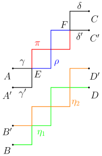
Figure 3.1. Illustration of the proof of Lemma 3.1. Here we show points  $E,F$  and paths  $\gamma,\gamma^{\prime},\delta,\delta^{\prime}$, $\pi$ (in red)  and $\rho$ (in blue). The green path $\eta_{1}$ is formed by following $\gamma^{\prime}$ then $\rho$ and then $\delta^{\prime}$ and translating the resulting path by $\operatorname{\mathbf{v}}$, so it is a path $B\to D$. The orange path $\eta_{2}$ is also shown.

Proof.

The idea is to consider the pairs of paths counted on each side, and show that each pair (after the necessary transformation) is counted less times on the RHS than on the LHS, where the number of times it could appear on each side is $0,1,2$.

To be precise, given two points $E$ and $F$ in $\operatorname{\textnormal{Reg}}(P)$ between the lines $AB$ and $CD$, and paths $(\pi,\rho)$ with endpoints $E$ and $F$, let

$$S(E,F)\ :=\ \big{\{}(\gamma,\hskip 1.70709pt\gamma^{\prime},\hskip 1.70709pt\delta,\hskip 1.70709pt\delta^{\prime})\ |\ \gamma:A\to E,\,\gamma^{\prime}:A^{\prime}\to E,\,\delta:F\to C,\,\delta^{\prime}:F\to C^{\prime}\big{\}}.$$

Here we have $4$-tuples of paths with the given endpoints, such that their only intersection points are the endpoints, namely  $\gamma\cap\gamma^{\prime}=\{E\}$  and   $\delta\cap\delta^{\prime}=\{F\}$. Connecting the paths in $S(E,F)$ with $(\pi,\rho)$, we can obtain four different pairs of paths from the points $A,A^{\prime}$ to $C,C^{\prime}$. We now count how often each such pair is counted in LHS and RHS of the desired inequality in (3.1), after we translate one of the paths by  $\operatorname{\mathbf{v}}:=\overrightarrow{AB^{\prime}}=\overrightarrow{A^{\prime}B}=\overrightarrow{C^{\prime}D}=\overrightarrow{CD^{\prime}}$.

Fix points $E,F$ as above, paths $\pi,\rho:E\to F$, and 4-tuple $(\gamma,\gamma^{\prime},\delta,\delta^{\prime})\in S(E,F)$. These 6 paths can be combined in different ways to give 2 paths from $A,A^{\prime}$ to $C,C^{\prime}$, and after translating one by $\operatorname{\mathbf{v}}$ obtain pairs appearing in (3.1). The pairs are:

$$\zeta_{1}\ :=\ \gamma\circ\pi\circ\delta,\qquad\zeta_{1}:A\to C\hskip 0.85355pt,\quad \eta_{1}\ :=\ (\gamma^{\prime}\circ\rho\circ\delta^{\prime})+\operatorname{\mathbf{v}},\qquad\eta_{1}:B\to D\hskip 0.85355pt,$$

$$\zeta_{2}\ :=\ \gamma^{\prime}\circ\pi\circ\delta^{\prime},\qquad\zeta_{2}:A^{\prime}\to C^{\prime}\hskip 0.85355pt,\quad \eta_{2}\ :=\ (\gamma\circ\rho\circ\delta)+\operatorname{\mathbf{v}},\qquad\eta_{2}:B^{\prime}\to D^{\prime}\hskip 0.85355pt,$$

$$\zeta_{3}\ :=\ \gamma\circ\pi\circ\delta^{\prime},\qquad\zeta_{3}:A\to C^{\prime}\hskip 0.85355pt,\quad \eta_{3}\ :=\ (\gamma^{\prime}\circ\rho\circ\delta)+\operatorname{\mathbf{v}},\qquad\eta_{3}:B\to D^{\prime}\hskip 0.85355pt,$$

$$\zeta_{4}\ :=\ \gamma^{\prime}\circ\pi\circ\delta,\qquad\zeta_{4}:A^{\prime}\to C\hskip 0.85355pt,\quad \eta_{4}\ :=\ (\gamma\circ\rho\circ\delta^{\prime})+\operatorname{\mathbf{v}},\qquad\eta_{4}:B^{\prime}\to D\hskip 0.85355pt.$$

Case 1:  At least one of $\zeta_{3},\eta_{3}$ is not (entirely contained) in $\operatorname{\textnormal{Reg}}(P)$, and at least one of $\zeta_{4},\eta_{4}$ is not in $\operatorname{\textnormal{Reg}}(P)$, then none of these pairs of paths is counted in the RHS of (3.1), and the contribution to the RHS is 0.

Case 2:  Both pairs of paths $(\zeta_{3},\eta_{4})$ and $(\zeta_{4},\eta_{4})$ are contained in $\operatorname{\textnormal{Reg}}(P)$. This implies that all the components and their translates are in $\operatorname{\textnormal{Reg}}(P)$, and hence  $\zeta_{1},\zeta_{2},\eta_{1},\eta_{2}\subset\operatorname{\textnormal{Reg}}(P)$. So the contribution from these paths is 2 on both LHS and RHS.

Case 3 and 4:  Exactly one pair is in $\operatorname{\textnormal{Reg}}(P)$, say $\zeta_{3},\eta_{3}\subset\operatorname{\textnormal{Reg}}(P)$ and at least one of $\zeta_{4},\eta_{4}$ is not in $\operatorname{\textnormal{Reg}}(P)$. Then $\gamma,\delta^{\prime},\gamma^{\prime}+\operatorname{\mathbf{v}},\delta+\operatorname{\mathbf{v}}\subset\operatorname{\textnormal{Reg}}(P)$. Since $\gamma^{\prime}$ is between $\gamma$ and $\gamma^{\prime}+\operatorname{\mathbf{v}}$, both of which are contained in $\operatorname{\textnormal{Reg}}(P)$, and since $\operatorname{\textnormal{Reg}}(P)$ is simply connected, we conclude that $\gamma^{\prime}$ is also in $\operatorname{\textnormal{Reg}}(P)$. Thus, $\zeta_{2}\subset\operatorname{\textnormal{Reg}}(P)$. Similarly, since $\gamma+\operatorname{\mathbf{v}}$ is between $\gamma$ and $\gamma^{\prime}+\operatorname{\mathbf{v}}$, we have $\gamma+\operatorname{\mathbf{v}}\subset\operatorname{\textnormal{Reg}}(P)$. Thus, $\zeta_{2},\eta_{2}\subset\operatorname{\textnormal{Reg}}(P)$. Hence these paths are counted once in the RHS and at least once in the LHS.

To finish the proof, we need to show that we have indeed considered all possible pairs of paths which can arise in the RHS. Let $\zeta\in\mathcal{K}(A^{\prime},C)$, $\eta\in\mathcal{K}(B^{\prime},D)$, so $(\eta,\zeta)$ is a pair of paths counted in the first term on the RHS. Let $\widehat{\eta}=\eta-\operatorname{\mathbf{v}}:A\to C^{\prime}$, it has to intersect $\zeta$. Let $E$ be the first intersection point (closest to $A/A^{\prime}$) and let $F$ be the last intersection point. Set $\pi=\zeta(E,F)$, $\rho=\widehat{\eta}(E,F)$ and $\gamma^{\prime}=\zeta(A^{\prime},E)$, $\gamma=\widehat{\eta}(A,E)$, $\delta^{\prime}=\widehat{\eta}(F,C^{\prime})$ and $\delta=\zeta(F,C)$. Then, fixing these $E,F,\pi,\rho$ and $(\gamma,\gamma^{\prime},\delta,\delta^{\prime})\in S(E,F)$ we recover $\zeta=\zeta_{4}$ and $\eta=\eta_{4}$. Similarly, given $\zeta\in\textrm{\em K}(A,C^{\prime})$ and $\eta\in\textrm{\em K}(B,D^{\prime})$ we recover $(\zeta_{3},\eta_{3})$.

Moreover, these constructions reassign portions of the same paths on the RHS and LHS, total translated areas cancel out, so the $q$-weights are preserved and the inequality holds for the $q$-weighted paths. This completes the proof. ∎

3.2. Equalities

Here we describe the cases when equalities in the lattice path lemmas from Section 2 are achieved. The following is an easy generalization of the [CPP21a, Lemma 8.4].

Lemma 3.2 (Equality lemma).

Let  $A,B,A^{\prime},B^{\prime},C,D\in\operatorname{\textnormal{Reg}}(P)$  be as in Lemma 2.3. We then have the following conditions for equalities in Lemma 2.3:  If  $a_{2}^{\prime}-b_{2}>c_{2}-d_{2}$ , then

$$\textrm{\em K}(A^{\prime},C)\,\cdot\,\textrm{\em K}(B^{\prime},D)\ =\ \textrm{\em K}(A,C)\,\cdot\,\textrm{\em K}(B,D)$$

if and only if either both sides are zero, or

$$\textrm{\em K}_{q}(A^{\prime},C)\ =\ \textrm{\em K}_{q}(A,C)\ \quad\text{and}\ \quad\textrm{\em K}_{q}(B^{\prime},D)\ =\ \textrm{\em K}_{q}(B,D).$$

Furthermore, if  $a_{2}>a_{2}^{\prime}$  and the segment $CD$ lies strictly to the right of segment $AB$, then the segment $AB$ is part of the lower boundary of $\operatorname{\textnormal{Reg}}(P)$.

Proof.

We assume that $a_{2}>a_{2}^{\prime}$ and the segment $CD$ lies strictly to the right of $AB$, as otherwise the lemma is straightforward. The equality in Lemma 2.3 implies that the map $\varkappa$ is a bijection. Let  $\xi:B^{\prime}\to D$  be the highest possible path in $\operatorname{\textnormal{Reg}}(P)$ and  $\eta:A^{\prime}\to C$  be the lowest possible path in $\operatorname{\textnormal{Reg}}(P)$, see Figure 3.2. Then these paths must be in the image of $\varkappa$, and their preimages are  $\widehat{\xi}:B\to D$  and $\widehat{\eta}:A\to C$. Let  $\operatorname{\mathbf{v}}=\overrightarrow{B^{\prime}A}$.

Following the construction of $\varkappa^{-1}$, we see that the paths $\eta$ and  $\xi+\operatorname{\mathbf{v}}$  must intersect, with $E$ the closest intersection point to $A$. By the minimality of $\eta$ and maximality of $\xi$ in $\operatorname{\textnormal{Reg}}(P)$, we have that  $\xi+\operatorname{\mathbf{v}}$  is on or above $\eta$. Since the endpoints of $\xi+\operatorname{\mathbf{v}}$ (i.e. $A$ and $D^{\prime}$) are strictly above the endpoints of $\eta$ (i.e. $A^{\prime}$ and $C$) by assumptions, we have $E$ is contained in lower boundary of $\operatorname{\textnormal{Reg}}(P)$. Since $\xi$ is below  $\xi+\operatorname{\mathbf{v}}$ and is above the lower boundary of  $\operatorname{\textnormal{Reg}}(P)$, we have $E$ is contained in $\xi$. Next, we observe that if  $E\not\in AB$, then  $\widehat{\eta}(A,E)$  is strictly above $\xi(B^{\prime},E)$, which contradicts the maximality of $\xi$ in $\operatorname{\textnormal{Reg}}(P)$. Thus $E$ is contained in $AB$ and is on or above $A$, and so the lower boundary of $\operatorname{\textnormal{Reg}}(P)$ contains the segment $AB$. This completes the proof. ∎

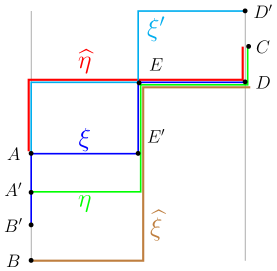
Figure 3.2. The proof of Lemma 3.2.

The following Lemma treats the special case when $A^{\prime}=B$ in the Equality Lemma 3.2. The inequality itself reduces directly to Lindström–Gessel–Viennot lemma as the translation vector  $\operatorname{\mathbf{v}}=\operatorname{\mathbf{0}}$.

Lemma 3.3 (Special equality lemma).

Let  $A,B\in\operatorname{\textnormal{Reg}}(P)$  be two points on the same vertical line with $A$ above $B$, and  $C,D\in\operatorname{\textnormal{Reg}}(P)$  points on another vertical line with $C$ above $D$ to the east of the line $AB$. Then:

$$\textrm{\em K}_{q}(A,C)\,\cdot\,\textrm{\em K}_{q}(B,D)\ \geqslant\ \textrm{\em K}_{q}(B,C)\,\cdot\,\textrm{\em K}_{q}(A,D)$$

with equality if and only if there exists a point $E$ for which every path counted here must pass through, i.e.,

$$\textrm{\em K}_{q}(A,C)\ =\ \textrm{\em K}_{q}(A,E)\hskip 1.70709pt\cdot\hskip 1.70709pt\textrm{\em K}_{q}(E,C),\qquad \textrm{\em K}_{q}(B,D)\ =\ \textrm{\em K}_{q}(B,E)\hskip 1.70709pt\cdot\hskip 1.70709pt\textrm{\em K}_{q}(E,D),$$

$$\textrm{\em K}_{q}(B,C)\ =\ \textrm{\em K}_{q}(B,E)\hskip 1.70709pt\cdot\hskip 1.70709pt\textrm{\em K}_{q}(E,C),\qquad \textrm{\em K}_{q}(A,D)\ =\ \textrm{\em K}_{q}(A,E)\hskip 1.70709pt\cdot\hskip 1.70709pt\textrm{\em K}_{q}(E,D).$$

Furthermore, if $CD$ lies strictly to the right of $AB$, then one of the three conditions hold:

• $E=A$  is part the lower boundary of  $\operatorname{\textnormal{Reg}}(P)$,

• $E=D$  is part of the upper boundary of  $\operatorname{\textnormal{Reg}}(P)$,

• $E$ is part of the upper and lower boundary of  $\operatorname{\textnormal{Reg}}(P)$.

Proof.

We assume that segment $CD$ lies strictly to the right of $AB$, as otherwise the lemma is straightforward. First, observe that the inequality follows from Lemma 2.3 by setting  $A^{\prime}\leftarrow A$,  $B^{\prime}\leftarrow B$  and  $A\leftarrow B$,  $B\leftarrow A$. In that case the translation vector is zero and we apply the intersection argument directly to the paths  $A\to C,B\to D$.

To analyze the equality, we notice that Lemma 3.2 does not apply anymore, so a different argument is needed. The “only if” part of the claim is clear. We now prove the if part. Let $\gamma:A\to C$ be the highest path within $\operatorname{\textnormal{Reg}}(P)$ from $A\to C$, and let $\delta:B\to D$ be the lowest possible path within $\operatorname{\textnormal{Reg}}(P)$ from $B$ to $D$. Since the injection $\varkappa$ in Lemma 2.3 is now a bijection, it follow that $\gamma$ and $\delta$ intersects at a point $E$. If $E$ is contained in the segment $AB$ (resp. $CD$), then the segment $AB$ (resp. $CD$) is contained in the lower (resp. upper) boundary of $\operatorname{\textnormal{Reg}}(P)$ and thus every path counted here must pass through $E=A$ (resp. $E=D$). If $E$ is not contained in the segment $AB$ or $CD$, then $E$ is an intersection of the upper and lower boundary of  $\operatorname{\textnormal{Reg}}(P)$, and every path in  $\operatorname{\textnormal{Reg}}(P)$  must pass through $E$. This completes the proof. ∎

4. Stanley’s log-concavity

Theorem 1.3 is a direct Corollary of Theorem 1.4 when setting $x$ to be a $\widehat{0}$ element in the poset. But its proof via lattice paths is much more direct, and illustrative, so we discuss it separately here first.

4.1. Proof of Theorem 1.3

Without loss of generality, assume  $x\in\mathcal{C}_{1}$, so $x=\alpha_{r}$ for some $r$. Let  $Y^{\langle k\rangle}=(r-1,k-r)$, so that the lattice paths corresponding to linear extensions $L$ with  $L(x)=k$  pass through  $A_{1}^{\prime}:=Y^{\langle k\rangle}$  and  $A^{\prime}:=Y^{\langle k\rangle}+\textbf{\hskip 0.85355pt{e}${}_{1}$}$. Let  $A:=Y^{\langle k+1\rangle}+\textbf{\hskip 0.85355pt{e}${}_{1}$}=A^{\prime}+\textbf{\hskip 0.85355pt{e}${}_{2}$}$,  $A_{1}:=Y^{\langle k+1\rangle}$,  $B_{1}:=Y^{\langle k-1\rangle}$,  $B:=B_{1}+\textbf{\hskip 0.85355pt{e}${}_{1}$}$. Then the paths with  $L(x)=k+1$  pass through $A_{1},A$ and the paths with  $L(x)=k-1$  pass through $B_{1},B$. We can then write the difference between the left and right hand sides of inequality (1.4) in terms of lattice paths as

(4.1) $$\begin{split}\Delta\,:=\,\textrm{N}_{q}(k)^{2}\,-\,\textrm{N}_{q}(k-1)\hskip 1.70709pt\cdot\hskip 1.70709pt\textrm{N}_{q}(k+1)\,=\,q^{2\binom{a+1}{2}+2k-2r}\,\times\qquad\qquad\qquad\\ \times\hskip 1.70709pt\biggl{[}\textrm{K}_{q}(\operatorname{\mathbf{0}},A_{1}^{\prime})^{2}\hskip 1.70709pt\textrm{K}_{q}(A^{\prime},Q)^{2}\,-\,\textrm{K}_{q}(\operatorname{\mathbf{0}},B_{1})\hskip 1.70709pt\textrm{K}_{q}(\operatorname{\mathbf{0}},A_{1})\hskip 1.70709pt\textrm{K}_{q}(B,Q)\hskip 1.70709pt\textrm{K}_{q}(A,Q)\biggr{]}\hskip 1.70709pt.\end{split}$$

We now apply Lemma 2.3 twice as follows. Let  $B_{1}^{\prime}=A_{1}^{\prime}$  and  $C=D=\operatorname{\mathbf{0}}$. Observe that this configuration matches the configuration in the Lemma by rotating  $\operatorname{\textnormal{Reg}}(P)$  by  $180^{\circ}$. Note that we can apply the lemma since  $\overrightarrow{A_{1}A_{1}^{\prime}}=-\overrightarrow{B_{1}B_{1}^{\prime}}=-\textbf{\hskip 0.85355pt{e}${}_{2}$}$  and  $a_{2}^{\prime}-b_{2}=1\geq 0=c_{2}-d_{2}$. Thus:

$$\textrm{K}_{q}(\operatorname{\mathbf{0}},A_{1}^{\prime})^{2}\ =\ \textrm{K}_{q}(\operatorname{\mathbf{0}},A_{1}^{\prime})\hskip 1.70709pt\cdot\hskip 1.70709pt\textrm{K}_{q}(\operatorname{\mathbf{0}},B_{1}^{\prime})\ \geqslant\ \textrm{K}_{q}(\operatorname{\mathbf{0}},A_{1})\hskip 1.70709pt\cdot\hskip 1.70709pt\textrm{K}_{q}(\operatorname{\mathbf{0}},B_{1}).$$

Similarly, on the other side we apply the lemma with  $A^{\prime}=B^{\prime}$  and  $C=D=Q$, satisfying the conditions since  $\overrightarrow{AA^{\prime}}=\textbf{\hskip 0.85355pt{e}${}_{2}$}=-\overrightarrow{BB^{\prime}}$  and  $a_{2}^{\prime}-b_{2}=1>0=c_{2}-d_{2}$. Thus:

$$\textrm{K}_{q}(A^{\prime},Q)^{2}\ =\ \textrm{K}_{q}(A^{\prime},Q)\hskip 1.70709pt\cdot\hskip 1.70709pt\textrm{K}_{q}(B^{\prime},Q)\ \geqslant\ \textrm{K}_{q}(A,Q)\hskip 1.70709pt\cdot\hskip 1.70709pt\textrm{K}_{q}(B,Q).$$

Multiplying the last two inequalities we obtain the desired inequality  $\Delta\geq 0$. ∎

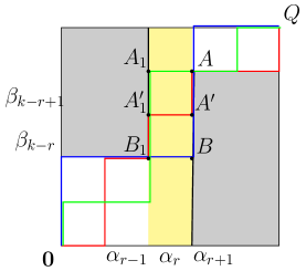
Figure 4.1. The equality case in Stanley’s Theorem 1.3 leading to the statement in Theorem 1.6, for the element $x=\alpha_{r}$ and $A_{1}^{\prime}=B_{1}^{\prime}=Y^{\langle k\rangle}$. The lattice paths equality Lemma 3.2 (after $180^{\circ}$ rotation) implies that all paths passing through $A_{1}$ also pass through $B_{1}$, so $A_{1}B_{1}$ is part of the upper boundary of $\operatorname{\textnormal{Reg}}(P)$ (shaded in gray). Similarly for the paths passing through $A,B$. We see that the square centered at $(r-1+\frac{1}{2},k-r+\frac{1}{2})\not\in\operatorname{\textnormal{Reg}}(P)$, which means that $\alpha_{r}\hskip 1.70709pt||\hskip 1.70709pt\beta_{k-r+1}$, and similarly we derive the other conditions.

4.2. Proof of Theorem 1.6

It is clear that (d) $\Rightarrow$ (c), (d) $\Rightarrow$ (b), (c) $\Rightarrow$ (a), and (b) $\Rightarrow$ (a). We now show that (a) $\Rightarrow$ (d). In the proof of the Stanley inequality, notice that the equality is achieved exactly when all applications of Lemma 2.3 lead to equalities. For the equality in the first application of Lemma 2.3, we have:

$$\textrm{K}_{q}(\operatorname{\mathbf{0}},A_{1}^{\prime})\,\textrm{K}_{q}(\operatorname{\mathbf{0}},B_{1}^{\prime})\ =\ \textrm{K}_{q}(\operatorname{\mathbf{0}},A_{1})\,\textrm{K}_{q}(\operatorname{\mathbf{0}},B_{1}).$$

This equality case is covered by Lemma 3.2 (after $180^{\circ}$ rotation), which implies that the segment  $A_{1}B_{1}$  is part of the upper boundary of  $\operatorname{\textnormal{Reg}}(P)$ (which is the condition after rotating by $180^{\circ}$). The second application of Lemma 2.3 implies that $AB$ is part of the lower boundary of  $\operatorname{\textnormal{Reg}}(P)$. Thus every path  $\operatorname{\mathbf{0}}\to Q$  passes on or below $B_{1}$ and on or above $A$. Hence  $q\textrm{N}_{q}(k-1)=\textrm{N}_{q}(k)=q^{-1}\textrm{N}_{q}(k-1)$, where the factors of $q$ arise from the different horizontal levels of the path passing from the  $A_{1}B_{1}$  segment to the $AB$ segment.

We now show that (a) $\Rightarrow$ (e). Since the lattice paths and  $\operatorname{\textnormal{Reg}}(P)$  correspond to the poset structure, we can restate the above conditions on poset level. The fact that  $A_{1}B_{1}$  is an upper boundary of  $\operatorname{\textnormal{Reg}}(P)$  implies that the element  $\beta_{k-r}\succ\alpha_{r-1}$. The fact that  $BB_{1},AA_{1}\subset\operatorname{\textnormal{Reg}}(P)$  implies that  $\beta_{k-r},\beta_{k-r+1}$  are not comparable to $\alpha_{r}$. Finally, $AB$ on the lower boundary of  $\operatorname{\textnormal{Reg}}(P)$  implies  $\alpha_{r+1}\succ\beta_{k+1-r}$.

We now show (e) $\Rightarrow$ (b) (cf. Proposition 8.8 for a proof of the analogous implication for Kahn–Saks equality for general posets). Denote  $\mathcal{N}(i):=\{L\in\operatorname{\mathcal{E}}(P)~{}:~{}L(x)=i\}$, so that  $\textrm{N}(i)=|\mathcal{N}(i)|$. Let $L\in\mathcal{N}(i)$. It follows from (e) that  $L(\beta_{k-r})=k-1$  and  $x\hskip 1.70709pt||\hskip 1.70709pt\beta_{k-r}$. Thus there is an injection  $\mathcal{N}(k)\to\mathcal{N}(k-1)$  by relabeling  $x\leftrightarrow\beta_{k-r}$, so that  $L(x)=k-1$ and $L(\beta_{k-r})=k$. Thus,  $\textrm{N}(k)\leq\textrm{N}(k-1)$. Similarly, we obtain  $\textrm{N}(k)\leq\textrm{N}(k+1)$  by relabeling  $x\leftrightarrow\beta_{k-r+1}$. However, by the Stanley inequality (Theorem 1.1), we have  $\textrm{N}(k)^{2}\hskip 0.85355pt\geq\hskip 0.85355pt\textrm{N}(k-1)\hskip 1.70709pt\textrm{N}(k+1)$, implying that all inequalities are in fact equalities. ∎

5. Proof of Theorem 1.4

For a given integer $w\in\mathbb{N}$, let  $\textrm{F}_{q}(w;k)$  be the $q$-weighted sum

$$\textrm{F}_{q}(w;k)\ :=\ \sum_{L}\,q^{\operatorname{\mathtt{wt}}(L)}\,,$$

where the sum is over all linear extensions  $L\in\operatorname{\mathcal{E}}(P)$, such that  $L(x)=w$  and  $L(y)=w+k$. By definition,

$$\textrm{F}_{q}(k)\ =\ \sum_{w\in\mathbb{N}}\,\textrm{F}_{q}(w;k)\hskip 0.85355pt.$$

We can thus express the difference

(5.1) $$\begin{split}\Delta\ :&=\ \textrm{F}_{q}(k)\hskip 1.70709pt\cdot\hskip 1.70709pt\textrm{F}_{q}(k)\ -\ \textrm{F}_{q}(k-1)\hskip 1.70709pt\cdot\hskip 1.70709pt\textrm{F}_{q}(k+1)\\ &=\ \sum_{v,\,v^{\prime}\in\operatorname{\mathbb{Z}}}\,\textrm{F}_{q}(v;k)\hskip 1.70709pt\cdot\hskip 1.70709pt\textrm{F}_{q}(v^{\prime};k)\ -\ \textrm{F}_{q}(v;k-1)\hskip 1.70709pt\cdot\hskip 1.70709pt\textrm{F}_{q}(v^{\prime};k+1)\\ &=\ \sum_{u>w-1}\hskip 1.70709ptS(u;w)\ +\ \frac{1}{2}\hskip 1.70709pt\sum_{u=w-1}\hskip 1.70709ptS(u;w),\end{split}$$

where we have grouped the terms in the expansions of products of  $\textrm{F}_{q}(*;*)$  using

(5.2) $$\begin{split}S(u;w)\ =&\ \textrm{F}_{q}(u;k)\hskip 1.70709pt\cdot\hskip 1.70709pt\textrm{F}_{q}(w;k)\,+\,\textrm{F}_{q}(w-1;k)\hskip 1.70709pt\cdot\hskip 1.70709pt\textrm{\em F}_{q}(u+1;k)\ \\ &-\ \textrm{F}_{q}(u;k+1)\hskip 1.70709pt\cdot\hskip 1.70709pt\textrm{F}_{q}(w;k-1)\,-\,\textrm{F}_{q}(u+1;k-1)\hskip 1.70709pt\cdot\hskip 1.70709pt\textrm{F}_{q}(w-1;k+1).\end{split}$$

In order to verify the identity (5.1), let  $u\geq w-1$. Note that by setting  $v\leftarrow w$,  $v^{\prime}\leftarrow u$  into the first term, and setting  $v\leftarrow u+1$,  $v^{\prime}\leftarrow w-1$  into the second term of (5.2), we cover the cases  $v^{\prime}\geq v-1$  and  $v\geq v^{\prime}+1$  in the positive summands in (5.1), where the double appearance of $v^{\prime}=v-1$ is balanced out by the factor $\frac{1}{2}$. Similarly, for the negative terms, setting  $v^{\prime}\leftarrow u$,  $v\leftarrow w$  covers the terms  $v^{\prime}\geq v-1$, and setting  $v^{\prime}\leftarrow w-1$,  $v\leftarrow u+1$  covers the terms  $v-1\geq v^{\prime}$. Formally, we have:

$$\sum_{u>w-1}\,\textrm{F}_{q}(u;k)\hskip 1.70709pt\cdot\hskip 1.70709pt\textrm{F}_{q}(w;k)\,+\,\textrm{F}_{q}(w-1;k)\hskip 1.70709pt\cdot\hskip 1.70709pt\textrm{F}_{q}(u+1;k)$$

$$\qquad=\ \sum_{v^{\prime}\geq v}\,\textrm{F}_{q}(v;k)\hskip 1.70709pt\cdot\hskip 1.70709pt{}\textrm{F}_{q}(v^{\prime};k)\ +\ \sum_{v\geq v^{\prime}+2}\,\textrm{F}_{q}(v;k)\hskip 1.70709pt\cdot\hskip 1.70709pt\textrm{F}_{q}(v^{\prime};k)$$

Similarly, we have:

$$\sum_{u>w-1}\,\textrm{F}_{q}(u;k+1)\hskip 1.70709pt\cdot\hskip 1.70709pt\textrm{F}_{q}(w;k-1)\,+\,\textrm{F}_{q}(u+1;k-1)\hskip 1.70709pt\cdot\hskip 1.70709pt\textrm{F}_{q}(w-1;k+1)$$

$$\qquad=\ \sum_{v^{\prime}\geq v}\,\textrm{F}_{q}(v^{\prime};k+1)\hskip 1.70709pt\cdot\hskip 1.70709pt\textrm{F}_{q}(v;k-1)\ +\ \sum_{v\geq v^{\prime}+2}\,\textrm{F}_{q}(v;k-1)\hskip 1.70709pt\cdot\hskip 1.70709pt\textrm{F}_{q}(v^{\prime};k+1),$$

and the remaining case of  $v^{\prime}=v-1$  comes from  $\frac{1}{2}S(u;u+1)$.

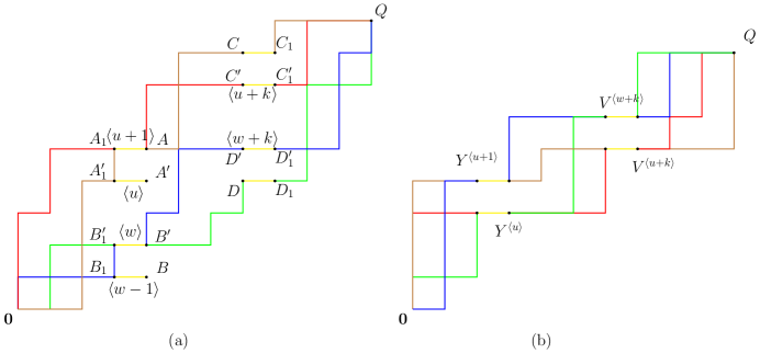
Figure 5.1. The proof of Theorem 1.4 in the case when $x,y\in\mathcal{C}_{1}$. Not all paths in $S(u;w)$ are drawn to avoid overcluttering. Figure (b) shows the paths involved in $S(u;u+1)$, which is the difference between the $q$-weighted sum of (red, blue) pairs minus the $q$-weighted sum of (green, brown) pairs.

We now prove that  $S(u;w)\geqslant 0$  for all  $u\geq w-1$  appearing in (5.1). Suppose  $x,y\in\mathcal{C}_{1}$  so  $x=\alpha_{s}$, and  $y=\alpha_{s+r}$. For  $u\in\operatorname{\mathbb{Z}}$, let  ${Y^{\langle u\rangle}}:=(s-1,u-s)$  and  ${V^{\langle u\rangle}}:=(s+r-1,u-(s+r))$, that is, if a linear extensions has $L(x)=w$ then its lattice path passes through $Y^{\langle w\rangle},Y^{\langle w\rangle}+\textbf{\hskip 0.85355pt{e}${}_{1}$}$, and if $L(y)=w+k$ then it passes through $V^{\langle w+k\rangle},V^{\langle w+k\rangle}+\textbf{\hskip 0.85355pt{e}${}_{1}$}$.

In terms of lattice paths, we have:

$$\textrm{F}_{q}(w;k)\ =\ q^{\binom{\emph{{a}}+1}{2}+2w+k}\,\textrm{K}_{q}\big{(}\operatorname{\mathbf{0}},Y^{\langle w\rangle}\big{)}\,\textrm{K}_{q}\bigl{(}Y^{\langle w\rangle}+\textbf{\hskip 0.85355pt{e}${}_{1}$},V^{\langle w+k\rangle}\bigr{)}\,\textrm{K}_{q}\bigl{(}V^{\langle w+k\rangle}+\textbf{\hskip 0.85355pt{e}${}_{1}$},Q\bigr{)}.$$

Let first $u>w-1$ and for simplicity label the following points $A_{1}=Y^{\langle u+1\rangle}$, $A=Y^{\langle u+1\rangle}+\textbf{\hskip 0.85355pt{e}${}_{1}$}$, $B_{1}=Y^{\langle w-1\rangle}$, $B=B_{1}+\textbf{\hskip 0.85355pt{e}${}_{1}$}$ and their shifts by $\pm\textbf{\hskip 0.85355pt{e}${}_{2}$}$ as $A^{\prime}_{1}={Y^{\langle u\rangle}}$, $A^{\prime}=A-\textbf{\hskip 0.85355pt{e}${}_{2}$}=A^{\prime}_{1}+\textbf{\hskip 0.85355pt{e}${}_{1}$}$, $B_{1}^{\prime}={Y^{\langle w\rangle}}$ and $B^{\prime}=B_{1}^{\prime}+\textbf{\hskip 0.85355pt{e}${}_{1}$}=B+\textbf{\hskip 0.85355pt{e}${}_{2}$}$. Similarly, let $C=V^{\langle u+k+1\rangle}$, $C_{1}=C+\textbf{\hskip 0.85355pt{e}${}_{1}$}$, $C^{\prime}=C-\textbf{\hskip 0.85355pt{e}${}_{2}$}=V^{\langle u+k\rangle}$, $C_{1}^{\prime}=C_{1}-\textbf{\hskip 0.85355pt{e}${}_{2}$}$ and $D=V^{\langle w+k-1\rangle}$, $D^{\prime}=D+\textbf{\hskip 0.85355pt{e}${}_{2}$}$ , $D_{1}=D+\textbf{\hskip 0.85355pt{e}${}_{1}$}$ and $D_{1}^{\prime}=D_{1}+\textbf{\hskip 0.85355pt{e}${}_{2}$}$.

Thus, letting  $\ell=2\binom{a+1}{2}+2u+2w+2k$, we can expand $S(u;w)$ and regroup its terms as follows:

(5.3) $$\begin{split}S(u;w)\hskip 1.70709ptq^{-\ell}\ =&\ \textrm{K}_{q}(\operatorname{\mathbf{0}},A_{1})\,\textrm{K}_{q}(\operatorname{\mathbf{0}},B_{1})\,\textrm{K}_{q}(A,C)\,\textrm{K}_{q}(B,D)\,\textrm{K}_{q}(C_{1},Q)\,\textrm{K}_{q}(D_{1},Q)\\ &\quad+\,\textrm{K}_{q}(\operatorname{\mathbf{0}},A^{\prime}_{1})\,\textrm{K}_{q}(\operatorname{\mathbf{0}},B^{\prime}_{1})\,\textrm{K}_{q}(A^{\prime},C^{\prime})\,\textrm{K}_{q}(B^{\prime},D^{\prime})\,\textrm{K}_{q}(C_{1}^{\prime},Q)\,\textrm{K}_{q}(D_{1}^{\prime},Q)\\ &\quad-\,\textrm{K}_{q}(\operatorname{\mathbf{0}},A_{1})\,\textrm{K}_{q}(\operatorname{\mathbf{0}},B_{1})\,\textrm{K}_{q}(A,C^{\prime})\,\textrm{K}_{q}(B,D^{\prime})\,\textrm{K}_{q}(C^{\prime}_{1},Q)\,\textrm{K}_{q}(D^{\prime}_{1},Q)\\ &\quad-\,\textrm{K}_{q}(\operatorname{\mathbf{0}},A^{\prime}_{1})\,\textrm{K}_{q}(\operatorname{\mathbf{0}},B^{\prime}_{1})\,\textrm{K}_{q}(A^{\prime},C)\,\textrm{K}_{q}(B^{\prime},D)\,\textrm{K}_{q}(C_{1},Q)\,\textrm{K}_{q}(D_{1},Q)\\ \ =&\ \Delta_{1}(\operatorname{\mathbf{0}};A_{1}/A^{\prime}_{1},B^{\prime}_{1}/B_{1})\,\Delta_{1}(A^{\prime},B^{\prime};C/C^{\prime},D^{\prime}/D;Q)\\ &\quad+\,\textrm{K}_{q}(\operatorname{\mathbf{0}},A_{1})\,\textrm{K}_{q}(\operatorname{\mathbf{0}},B_{1})\,\Delta_{1}(A/A^{\prime},B^{\prime}/B;C^{\prime},D^{\prime})\,\Delta_{1}(C/C^{\prime},D^{\prime}/D;Q)\\ &\quad+\,\textrm{K}_{q}(\operatorname{\mathbf{0}},A_{1})\,\textrm{K}_{q}(\operatorname{\mathbf{0}},B_{1})\,\Delta_{2}(A,B;C,D)\,\textrm{K}_{q}(C_{1},Q)\,\textrm{K}_{q}(D_{1},Q).\end{split}$$

Here the $\Delta$ notation means that we take differences of paths passing through either $E$ or $E^{\prime}$ when using the $E/E^{\prime}$, and $\Delta_{2}$ plays the role of a second derivative. Specifically, the restructured terms above are given as follows, they are each nonnegative by our lattice paths lemmas:

$$\Delta_{1}(\operatorname{\mathbf{0}};A_{1}/A^{\prime}_{1},B^{\prime}_{1}/B_{1})\ :=\ \textrm{K}_{q}(\operatorname{\mathbf{0}},A_{1}^{\prime})\,\textrm{K}_{q}(\operatorname{\mathbf{0}},B_{1}^{\prime})\,-\,\textrm{K}_{q}(\operatorname{\mathbf{0}},A_{1})\,\textrm{K}_{q}(\operatorname{\mathbf{0}},B_{1})\ \geqslant_{\text{Lem}~{}\ref{l:lattice path bijection 1}}\ 0,$$

$$\Delta_{1}(A^{\prime},B^{\prime};C/C^{\prime},D^{\prime}/D;Q)\ :=\ \textrm{K}_{q}(A^{\prime},C^{\prime},Q)\,\textrm{K}_{q}(B^{\prime},D^{\prime},Q)\,-\,\textrm{K}_{q}(A^{\prime},C,Q)\,\textrm{K}_{q}(B^{\prime},D,Q)\ \geqslant_{\text{(see below)}}\ 0,$$

$$\Delta_{1}(C_{1}/C^{\prime}_{1},D^{\prime}_{1}/D_{1};Q)\ :=\ \textrm{K}_{q}(C^{\prime}_{1},Q)\,\textrm{K}_{q}(D^{\prime}_{1},Q)\,-\,\textrm{K}_{q}(C_{1},Q)\,\textrm{K}_{q}(D_{1},Q)\ \geqslant_{\text{Lem}~{}\ref{l:lattice path bijection 1}}\ 0,$$

$$\Delta_{1}(A/A^{\prime},B^{\prime}/B;C^{\prime},D^{\prime})\ :=\ \textrm{K}_{q}(A^{\prime},C^{\prime})\,\textrm{K}_{q}(B^{\prime},D^{\prime})\,-\,\textrm{K}_{q}(A,C^{\prime})\,\textrm{K}_{q}(B,D^{\prime})\ \geqslant_{\text{Lem}~{}\ref{l:lattice path bijection 1}}\ 0,$$

$$\Delta_{2}(A,B;C,D)\ :=\ \textrm{K}_{q}(A,C)\,\textrm{K}_{q}(B,D)\,+\,\textrm{K}_{q}(A^{\prime},C^{\prime})\,\textrm{K}_{q}(B^{\prime},D^{\prime})$$

$$\qquad-\,\textrm{K}_{q}(A,C^{\prime})\,\textrm{K}_{q}(B,D^{\prime})\,-\,\textrm{K}_{q}(A^{\prime},C)\,\textrm{K}_{q}(B^{\prime},D)\ \geqslant_{\text{Lem}~{}\ref{l:path-averages}}\ 0.$$

Here the second inequality follows by applying Lemma 2.3 twice:

$$\textrm{K}_{q}(A^{\prime},C^{\prime})\ \textrm{K}_{q}(B^{\prime},D^{\prime})\ \geqslant\ \textrm{K}_{q}(A^{\prime},C)\ \textrm{K}_{q}(B^{\prime},D)\quad\text{ and }\quad\textrm{K}_{q}(C^{\prime}_{1},Q)\ \textrm{K}_{q}(D^{\prime}_{1},Q)\ \geqslant\ \textrm{K}_{q}(C_{1},Q)\ \textrm{K}_{q}(D_{1},Q).$$

Now let  $u=w-1$, we set  $Y^{\prime}:={Y^{\langle u\rangle}}+\textbf{\hskip 0.85355pt{e}${}_{1}$}$  and  $Y:={Y^{\langle w\rangle}}+\textbf{\hskip 0.85355pt{e}${}_{1}$}=Y^{\langle u+1\rangle}+\textbf{\hskip 0.85355pt{e}${}_{1}$}=Y^{\prime}+\textbf{\hskip 0.85355pt{e}${}_{2}$}$, and  $V^{\prime}:=V^{\langle u+k\rangle}$  and  $V:=V^{\langle u+k+1\rangle}=V^{\prime}+\textbf{\hskip 0.85355pt{e}${}_{2}$}$. Then:

(5.4) $$\frac{1}{2}\hskip 1.70709ptS(u;u+1) =\,\textrm{F}_{q}(u;k)\,\textrm{F}_{q}(u+1;k)\,-\,\textrm{F}_{q}(u;k+1)\,\textrm{F}_{q}(u+1;k-1)$$

$$=\,q^{2\binom{\emph{{a}}+1}{2}+4u+2+2k}\,\textrm{K}_{q}\big{(}\operatorname{\mathbf{0}},{Y^{\langle w\rangle}}\big{)}\,\textrm{K}_{q}\big{(}\operatorname{\mathbf{0}},{Y^{\langle u\rangle}}\big{)}\,\textrm{K}_{q}\big{(}V+\textbf{\hskip 0.85355pt{e}${}_{1}$},Q\big{)}\,\textrm{K}_{q}\big{(}V^{\prime}+\textbf{\hskip 0.85355pt{e}${}_{1}$},Q\big{)}\ \times$$

$$\qquad\qquad\times\ \biggl{[}\textrm{K}_{q}(Y,V)\,\textrm{K}_{q}(Y^{\prime},V^{\prime})\,-\,\textrm{K}_{q}(Y^{\prime},V)\,\textrm{K}_{q}(Y,V^{\prime})\biggr{]}\ \geqslant_{\text{Lem~{}\ref{l: lgv}}}\ 0\hskip 0.85355pt.$$

This completes the proof. ∎

6. Proof of Theorem 1.7

6.1. Setting up the proof

It is clear that  (d) $\Rightarrow$ (c),  (d) $\Rightarrow$ (b),  (c) $\Rightarrow$ (a), and  (b) $\Rightarrow$ (a).

For  (e) $\Rightarrow$ (d), we adapt the proof of Proposition 8.8 below, of the analogous implication for general posets. Without loss of generality, we assume that $z=x$ and $x\in\mathcal{C}_{1}$. Then (e) implies that, given a linear extension  $L\in\operatorname{\mathcal{E}}(P)$  with  $L(y)-L(x)=k$, we can obtain linear extension  $L^{\prime}\in\operatorname{\mathcal{E}}(P)$  with  $L^{\prime}(y)-L^{\prime}(x)=k-1$, and linear extension  $L^{\prime\prime}\in\operatorname{\mathcal{E}}(P)$  with  $L^{\prime\prime}(y)-L^{\prime\prime}(x)=k+1$, by switching element $x$ with the succeeding and preceding element in $L$, respectively. This map is clearly an injection that changes the $q$-weight by a factor of  $q^{\pm 1}$, so we have

$$\textrm{F}_{q}(k-1)\ \geqslant\ q\hskip 1.70709pt\textrm{F}(k)\quad\text{and}\quad\textrm{F}_{q}(k+1)\ \geqslant\ q^{-1}\hskip 1.70709pt\textrm{F}(k).$$

Since we also have  $\textrm{F}_{q}(k)^{2}\geq\textrm{F}_{q}(k-1)\textrm{F}_{q}(k+1)$  by Kahn–Saks Theorem 1.4, we conclude that equality occurs in the equation above, which proves (d).

The proof of  (a) $\Rightarrow$ (e)  will occupy the rest of this section. Together with the implications above, this implies the theorem.

6.2. Lattice paths interpretation

Suppose that $x=\alpha_{s}$ and $y=\alpha_{s+r}$. We will assume without loss of too much generality that $r>1$, so that the boundary between the region of $x$ and the region of $y$ does not overlap. This allows us to apply the combinatorial interpretation in Lemma 3.2 and Lemma 3.3. We remark that the method described here still applies to the case $r=1$ (by a slight modification of Lemma 3.2 and Lemma 3.3), and we omit the details here for brevity.

The idea of the proof is as follows. Informally, we will show that condition (a) implies that the regions above $x$ or $y$ is a vertical strip of width 1, that is the upper and lower boundary above $x$ and above $y$ are at distance 1 from each other, see Figure 4.1. These strips extend to the levels for which there exist a linear extension  $L\in\operatorname{\mathcal{E}}(P)$  with  $L(y)-L(x)=k\pm 1$ (see the full proof for precise description in each possible case). In order to show this, we analyze the proof of Theorem 1.4 in Section 5. In order to have equality we must have  $S(u;w)=0$  for every  $u\geq w-1$. So we apply the equality conditions from Lemmas 3.2 and 3.3 for every inequality involved in the proofs of  $S(u;w)\geq 0$. These equality conditions impose restrictions on the boundaries of  $\operatorname{\textnormal{Reg}}(P)$, making them vertical at the relevant levels above $x$ and $y$, and ultimately drawing the width-1 vertical strip. This analysis requires choosing special points  $u$ and $w$ from Section 5, and the application of the equality Lemmas requires certain conditions. Thus there are several different cases which need to be considered.

In order to apply this analysis we parameterize  $\operatorname{\textnormal{Reg}}(P)$  above $x$ and $y$ as follows. Let $u_{0}$ be the smallest possible value  $L(x)=L(\alpha_{s})$  can take, i.e.  $(Y^{\langle u_{0}\rangle},Y^{\langle u_{0}\rangle}+\textbf{\hskip 0.85355pt{e}${}_{1}$})$  is a segment in the lower boundary of  $\operatorname{\textnormal{Reg}}(P)$, see Figure 6.1. Let  $u_{1}-1$  be the largest possible value that  $L(\alpha_{s-1})$  can take, i.e.  $(Y^{\langle u_{1}\rangle}-\textbf{\hskip 0.85355pt{e}${}_{1}$},Y^{\langle u_{1}\rangle})$  is a segment in the upper boundary of  $\operatorname{\textnormal{Reg}}(P)$. Let  $u_{2}+1$  be the smallest possible value  $L(\alpha_{s+1})$  can take, i.e.  $(Y^{\langle u_{2}\rangle}+\textbf{\hskip 0.85355pt{e}${}_{1}$},Y^{\langle u_{2}\rangle}+2\textbf{\hskip 0.85355pt{e}${}_{1}$})$  is a segment in the lower boundary of  $\operatorname{\textnormal{Reg}}(P)$. Finally, let $u_{3}$ be the largest possible value $L(x)$ can take, so  $(Y^{\langle u_{3}\rangle},Y^{\langle u_{3}\rangle}+\textbf{\hskip 0.85355pt{e}${}_{1}$})$  is a segment in the upper boundary of $\operatorname{\textnormal{Reg}}(P)$. Clearly we have  $u_{0}\leq u_{1}$  and  $u_{2}\leq u_{3}$. Similarly, let  $w_{0}+k$  be the smallest possible value  $L(y)$  can take, so this gives the level of the lower boundary of $\operatorname{\textnormal{Reg}}(P)$ above $y$. Finally, let  $w_{1}+k-1$  be the largest possible value  $L(\alpha_{r+s-1})$  can take, let  $w_{2}+k+1$  be the smallest possible value  $L(\alpha_{r+s+1})$  can take, and  $w_{3}+k$  be the largest possible value  $L(y)$  can take. Clearly, we have  $w_{0}\leq w_{1}$  and  $w_{2}\leq w_{3}$.

Here we are only concerned with effectively possible values of $u$, i.e.  values for which there exist linear extensions with  $L(x)=u$  and  $L(y)-L(x)\in[k-1,k+1]$. We can thus restrict our region above $x$ and $y$, as follows. If we had  $w_{0}-u_{0}>1$, then  $\textrm{F}(u_{0};j)=0$  for  $j\in\{k-1,k,k+1\}$, since $L(y)\leq u_{0}+k+1<w_{0}+k$. Thus we can assume that the region above $x$ starts at  $L(x)=w_{0}-1$. Similarly, if  $w_{0}-u_{0}<-1$, we can restrict the region above $y$ accordingly. Thus we can assume  $|w_{0}-u_{0}|\leq 1$. Similarly, we can apply the same argument to the upper boundaries, and assume that  $|w_{3}-u_{3}|\leq 1$. Finally, let  $\operatorname{v_{\textnormal{max}}}$  be the largest integer such that  $\textrm{F}(\operatorname{v_{\textnormal{max}}};k)>0$, and let  $\operatorname{v_{\textnormal{min}}}$  be the smallest integer such that  $\textrm{F}(\operatorname{v_{\textnormal{min}}};k)>0$. Note that  $\operatorname{v_{\textnormal{max}}}=\min\{u_{3},w_{3}\}$  and  $\operatorname{v_{\textnormal{min}}}=\max\{u_{0},w_{0}\}$.

Figure 6.1. The structure of $\operatorname{\textnormal{Reg}}(P)$ in the analysis of the Kahn–Saks equality. Here  $k=5$, $u_{0}=5$, $u_{1}=6$, $u_{2}=7$, $u_{3}=8$,  and  $w_{0}=5$, $w_{1}=6$, $w_{2}=8$, $w_{3}=9$.

In the language of lattice paths, condition (e) follows from showing either of the following:

1. For every  $v\in[\operatorname{v_{\textnormal{min}}},\operatorname{v_{\textnormal{max}}}]$, we have $Y^{\langle v-1\rangle}$ is contained in the upper boundary of $\operatorname{\textnormal{Reg}}(P)$, and $Y^{\langle v+1\rangle}+\textbf{\hskip 0.85355pt{e}${}_{1}$}$ is contained in the lower boundary of $\operatorname{\textnormal{Reg}}(P)$.

2. For every  $v\in[\operatorname{v_{\textnormal{min}}},\operatorname{v_{\textnormal{max}}}]$, we have $Y^{\langle v+k-1\rangle}$ is contained in the upper boundary of $\operatorname{\textnormal{Reg}}(P)$, and $Y^{\langle v+k+1\rangle}+\textbf{\hskip 0.85355pt{e}${}_{1}$}$ is contained in the lower boundary of $\operatorname{\textnormal{Reg}}(P)$.

Note that these condition imply the width-1 vertical strip above $x$ or $y$ for all relevant values. It also implies that  $L^{-1}(v\pm 1)\in\mathcal{C}_{2}$  and that  $L^{-1}(v\pm 1)\hskip 1.70709pt||\hskip 1.70709ptx$  since  $Y^{\langle v\pm 1\rangle},\hskip 1.70709ptY^{\langle v\pm 1\rangle}+\textbf{\hskip 0.85355pt{e}${}_{1}$}\in\operatorname{\textnormal{Reg}}(P)$.

For the rest of the section, we write  $A^{\prime}:=Y^{\langle u\rangle}$,  $B^{\prime}:=Y^{\langle w\rangle}$, and let the notations  $A,B,A_{1},B_{1},A_{1}^{\prime},B_{1}^{\prime}$, $C,D,C^{\prime},D^{\prime},C_{1},D_{1},C_{1}^{\prime},D_{1}^{\prime}$  be as in the proof of Theorem 1.4 in Section 5. The choices of $u$ and $w$ will be chosen separately for each case of consideration. We also write  $m:=u_{3}-u_{0}$  and  $m^{\prime}:=w_{3}-w_{0}$.

We split the proof into different cases, depending on the values of  $m$, $m^{\prime}$, $u_{1}-u_{0}$, $w_{3}-w_{2}$, $u_{0}-w_{0}$, and  $u_{3}-w_{3}$.

6.3. The cases $m\geq 2$, $u_{0}<u_{1}$ or $m^{\prime}\geq 2$, $w_{2}<w_{3}$.

We will now prove that (S2) holds for the first case. The second case is analogous, after  $180^{\circ}$  rotation of the configuration, and leads to (S1).

Note that  $\textrm{F}(u_{0}+1;k)>0$  since there is a linear extensions  $L(x)=u_{0}+1$  and  $L(y)=u_{0}+k+1\in[w_{0}+k,w_{3}+k]$. We then have:

$$u_{0}\ \leq\ \operatorname{v_{\textnormal{min}}}\ \leq\ u_{0}+1\ \leq\ u_{1}\qquad\text{and}\qquad u_{0}+1\ \leq\ \operatorname{v_{\textnormal{max}}}\ \leq u_{3}\hskip 1.70709pt.$$

We now turn to the proof of the inequality in Section 5, and notice that equality in (1.2) would be achieved only if  $S(u;w)=0$. Let  $u:=\operatorname{v_{\textnormal{max}}}$  and  $w:=\operatorname{v_{\textnormal{min}}}$. Since  $S(u;w)=0$, this means that

$$\Delta_{1}(\operatorname{\mathbf{0}};A_{1}/A^{\prime}_{1},B^{\prime}_{1}/B_{1})\,=\,0\qquad \text{or}\qquad\Delta_{1}(A^{\prime},B^{\prime};C/C^{\prime},D^{\prime}/D;Q)\,=\,0.$$

Now note that by Lemma 3.2 we must have  $\Delta_{1}(\operatorname{\mathbf{0}};A_{1}/A^{\prime}_{1},B^{\prime}_{1}/B_{1})>0$, since the condition of $A_{1}B_{1}$ being part of $\operatorname{\textnormal{Reg}}(P)$’s boundary is not satisfied: $B_{1}=Y^{\langle w-1\rangle}$ is not part of the upper boundary of $\operatorname{\textnormal{Reg}}(P)$ since $w\leq u_{1}$. Thus we must have $\Delta_{1}(A^{\prime},B^{\prime};C/C^{\prime},D^{\prime}/D;Q)=0$. This implies that

(6.1) $$\textrm{K}(A^{\prime},C^{\prime})\,\textrm{K}(B^{\prime},D^{\prime})\,\textrm{K}(C_{1}^{\prime},Q)\,\textrm{K}(D^{\prime}_{1},Q)\ =\ \textrm{K}(A^{\prime},C)\,\textrm{K}(B^{\prime},D)\,\textrm{K}(C_{1},Q)\,\textrm{K}(D_{1},Q).$$

Let us show that every terms in the left side of (6.1) is nonzero. Suppose otherwise, that  $\textrm{K}(A^{\prime},C^{\prime})=0$ (the other cases are treated analogously). By the monotonous boundaries of  $\operatorname{\textnormal{Reg}}(P)$, we must have $A^{\prime}$ or $C^{\prime}$ not in  $\operatorname{\textnormal{Reg}}(P)$, contradicting the choice of $u$ since there are linear extensions with  $L(x)=u$  and  $L(y)=y+k$.

Therefore, we must have equality in both applications of Lemma 2.3, so we can apply the Equality Lemma 3.2 to both terms in (6.1) (one after $180^{\circ}$ rotation). These equalities imply that  $CD=Y^{\langle\operatorname{v_{\textnormal{max}}}+k+1\rangle}\,Y^{\langle\operatorname{v_{\textnormal{min}}}+k-1\rangle}$  is part of the upper boundary of $\operatorname{\textnormal{Reg}}(P)$, and that  $C_{1}D_{1}=(Y^{\langle\operatorname{v_{\textnormal{max}}}+k+1\rangle}+\textbf{\hskip 0.85355pt{e}${}_{1}$})\,(Y^{\langle\operatorname{v_{\textnormal{min}}}+k-1\rangle}+\textbf{\hskip 0.85355pt{e}${}_{1}$})$  is part of the lower boundary of $\operatorname{\textnormal{Reg}}(P)$. This implies (S2).

For the rest of the proof, we can assume that $w_{2}=w_{3}$ if $m^{\prime}\geq 2$ and $u_{0}=u_{1}$ if $m\geq 2$.

6.4. The case $m\geq 2$, $u_{0}=u_{1}$, $u_{3}>w_{3}$

Since $u_{3}>w_{3}$, we have that $w_{3}=\operatorname{v_{\textnormal{max}}}$ and $u_{3}=\operatorname{v_{\textnormal{max}}}+1$. Let $u:=\operatorname{v_{\textnormal{max}}}$ and $w:=\operatorname{v_{\textnormal{max}}}$. Since $m\geq 2$ we have that $A_{1},B_{1}\in\operatorname{\textnormal{Reg}}(P)$, and since $w_{3}<u_{3}$ we have that $CC_{1}\not\in\operatorname{\textnormal{Reg}}(P)$. Thus we have:

$$\textrm{K}(\operatorname{\mathbf{0}},A_{1}),\,\textrm{K}(\operatorname{\mathbf{0}},B_{1}),\,\textrm{K}(C_{1}^{\prime},Q),\,\textrm{K}(D_{1}^{\prime},Q)\ >\ 0\qquad\text{and}\qquad\textrm{K}(A,C)=\textrm{K}(A^{\prime},C)\ =\ 0.$$

We will first show that the segment $AB$ is contained in the lower boundary of $\operatorname{\textnormal{Reg}}(P)$.

Since $S(u;w)=0$, the vanishing of the second summand in (5.3) implies that either

$$\textrm{K}(\operatorname{\mathbf{0}},A_{1})\hskip 1.70709pt\cdot\hskip 1.70709pt\textrm{K}(\operatorname{\mathbf{0}},B_{1})=0,\ \quad\text{or}\ \quad\Delta_{1}(C_{1}/C^{\prime}_{1},D^{\prime}_{1}/D_{1};Q)=0,\ \quad\text{or}\ \quad\Delta_{1}(A/A^{\prime},B^{\prime}/B;C^{\prime},D^{\prime})=0.$$

The first product is nonzero from above. Below we show that  $\Delta_{1}(C_{1}/C^{\prime}_{1},D^{\prime}_{1}/D_{1};Q)\neq 0$, implying that  $\Delta_{1}(A/A^{\prime},B^{\prime}/B;C^{\prime},D^{\prime})=0$.

Note that the expression for $S(u;w)$ is implicitly over paths containing the entire horizontal segments above $x,y$. That is, in equation 5.3, there is a summand containing $\textrm{K}(*,C)$ if and only if it also contains $\textrm{K}(C_{1},Q)$, because the whole expression counts paths passing through $CC_{1}$. Thus, we can replace $\textrm{K}(C_{1},Q)$ everywhere by $\widehat{\textrm{K}}(C_{1},Q):=\textrm{K}(C,C_{1},Q)$. With this replacement we have that $\widehat{\textrm{K}}(C_{1},Q)=0$ since $C\not\in\operatorname{\textnormal{Reg}}(P)$ and so:

$$\textrm{K}(C^{\prime}_{1},Q)\hskip 1.70709pt\cdot\hskip 1.70709pt\textrm{K}(D^{\prime}_{1},Q)\ >\ 0\ =\ \widehat{\textrm{K}}(C_{1},Q)\hskip 1.70709pt\cdot\hskip 1.70709pt\textrm{K}(D_{1},Q).$$

This implies that  $\Delta_{1}(C_{1}/C^{\prime}_{1},D^{\prime}_{1}/D_{1};Q)\neq 0$, and, therefore,  $\Delta_{1}(A/A^{\prime},B^{\prime}/B;C^{\prime},D^{\prime})=0$. This in turn implies that $AB$ is contained in the lower boundary of  $\operatorname{\textnormal{Reg}}(P)$  by the Equality Lemma 3.2.

Now note that, since $AB$ is in the lower boundary of  $\operatorname{\textnormal{Reg}}(P)$, every path in  $\operatorname{\textnormal{Reg}}(P)$  must pass through  $A=Y^{\langle\operatorname{v_{\textnormal{max}}}+1\rangle}+\textbf{\hskip 0.85355pt{e}${}_{1}$}=Y^{\langle u_{3}\rangle}+\textbf{\hskip 0.85355pt{e}${}_{1}$}$. Also note that, since $u_{0}=u_{1}$, we have  $Y^{\langle u_{0}\rangle}\,Y^{\langle u_{0}+1\rangle}$  is in the upper boundary of  $\operatorname{\textnormal{Reg}}(P)$, so every path in  $\operatorname{\textnormal{Reg}}(P)$  must pass through $Y^{\langle u_{0}\rangle}$. These two properties imply that paths differ only by the level of their horizontal segment above $x$ and so

(6.2) $$\begin{split}\textrm{F}(v;k-1)\ &=\ \textrm{F}(v-1;k)\quad\text{ for every }\quad v\in[u_{0}+1,u_{3}]\hskip 1.70709pt,\\ \textrm{F}(v;k+1)\ &=\ \textrm{F}(v+1;k)\quad\text{ for every }\quad v\in[u_{0},u_{3}-2]\hskip 1.70709pt.\end{split}$$

We will use  (6.2) to show that  $\operatorname{v_{\textnormal{min}}}=u_{0}+1$.

Suppose first that $\operatorname{v_{\textnormal{min}}}=u_{0}$. Then (6.2) gives us

$$\textrm{F}(k-1)\ =\ \sum_{v=u_{0}+1}^{u_{3}}\,\textrm{F}(v;k-1)\ =\ \sum_{v=u_{0}+1}^{u_{3}}\,\textrm{F}(v-1;k)\ =\ \sum_{v=u_{0}}^{u_{3}-1}\,\textrm{F}(v;k)\ =\ \textrm{F}(k),$$

$$\textrm{F}(k+1)\ =\ \sum_{v=u_{0}}^{u_{3}-2}\,\textrm{F}(v;k+1)\ =\ \sum_{v=u_{0}}^{u_{3}-2}\,\textrm{F}(v+1;k)\ =\ \sum_{v=u_{0}+1}^{u_{3}-1}\,\textrm{F}(v;k)\ <\ \textrm{F}(k).$$

So we have  $\textrm{F}(k)^{2}>\textrm{F}(k-1)\hskip 1.70709pt\textrm{F}(k+1)$, a contradiction.

Then suppose that $\operatorname{v_{\textnormal{min}}}=u_{0}-1$. Then (6.2) gives us

$$\textrm{F}(k-1)\ =\ \sum_{v=u_{0}}^{u_{3}}\textrm{F}(v;k-1)\ =\ \sum_{v=u_{0}+1}^{u_{3}}\textrm{F}(v-1;k)\ +\ \textrm{F}(u_{0};k-1)\ =\ \sum_{v=u_{0}}^{u_{3}-1}\textrm{F}(v;k)\,+\,\textrm{F}(u_{0};k-1)$$

$$=\ \textrm{F}(k)\ +\ \textrm{F}(u_{0};k-1),$$

$$\textrm{F}(k+1)\ =\ \sum_{v=u_{0}}^{u_{3}-2}\textrm{F}(v;k+1)\ =\ \sum_{v=u_{0}}^{u_{3}-2}\textrm{F}(v+1;k)\ =\ \sum_{v=u_{0}+1}^{u_{3}-1}\textrm{F}(v;k)\ =\ \textrm{F}(k)\,-\,\textrm{F}(u_{0};k).$$

On the other hand, since  $\operatorname{v_{\textnormal{min}}}=u_{0}-1$  and  $\operatorname{v_{\textnormal{max}}}=u_{3}-1$, we then have  $m^{\prime}=m\geq 2$, so we can without loss of generality assume that  $w_{2}=w_{3}$ from the conclusion of the previous subsection. Since  $w_{2}=w_{3}$, we then have:

$$\textrm{F}(u_{0};k-1)\ \leq\ \textrm{F}(u_{0};k).$$

Combining these two equations, we then have

$$\textrm{F}(k-1)\hskip 1.70709pt\cdot\hskip 1.70709pt\textrm{F}(k+1)\ =\ \big{[}\textrm{F}(k)+\textrm{F}(u_{0};k-1)\big{]}\hskip 1.70709pt\cdot\hskip 1.70709pt\big{[}\textrm{F}(k)-\textrm{F}(u_{0};k)\big{]}\ \leq\ \textrm{F}(k)^{2}\ -\ \textrm{F}(u_{0};k)^{2}\ <\ \textrm{F}(k)^{2}\hskip 1.70709pt,$$

which is another contradiction. Hence, since  $\operatorname{v_{\textnormal{min}}}\in[u_{0}-1,u_{0}+1]$, we conclude that we must have  $\operatorname{v_{\textnormal{min}}}=u_{0}+1$.

Now recall that the combinatorial properties say that  $Y^{\langle u_{0}\rangle}=Y^{\langle\operatorname{v_{\textnormal{min}}}-1\rangle}$  is contained in the upper boundary of  $\operatorname{\textnormal{Reg}}(P)$, and  $Y^{\langle\operatorname{v_{\textnormal{max}}}+1\rangle}+\textbf{\hskip 0.85355pt{e}${}_{1}$}$  is contained in the lower boundary of  $\operatorname{\textnormal{Reg}}(P)$. This implies (S1), as desired.

An analogous conclusion can be derived for the case $u_{0}>w_{0}$ by applying the same argument. Finally, by the 180^∘ rotation, an analogous conclusion can be drawn for the case  $u_{3}<w_{3}$  and/or  $u_{0}<w_{0}$. Hence for the rest of the proof we can assume that  $u_{0}=w_{0}$  and  $u_{3}=w_{3}$  if  $m\geq 2$.

6.5. The case $m\geq 2$, $u_{0}=u_{1}$, $w_{2}=w_{3}$, $u_{0}=w_{0}$, $u_{3}=w_{3}$

Note that in this case  $m=u_{3}-u_{0}=w_{3}-w_{0}=m^{\prime}$,  $\operatorname{v_{\textnormal{min}}}=u_{0}=w_{0}$  and  $\operatorname{v_{\textnormal{max}}}=u_{3}=w_{3}$. We will show that this case leads to a contradiction.

Claim: Either the segment $(Y^{\langle\operatorname{v_{\textnormal{max}}}\rangle}+\textbf{\hskip 0.85355pt{e}${}_{1}$},Y^{\langle\operatorname{v_{\textnormal{min}}}\rangle}+\textbf{\hskip 0.85355pt{e}${}_{1}$})$ is contained in the lower boundary of $\operatorname{\textnormal{Reg}}(P)$, or the segment $(V^{\langle\operatorname{v_{\textnormal{max}}}+k\rangle},V^{\langle\operatorname{v_{\textnormal{min}}}+k\rangle})$ is contained in the upper boundary of $\operatorname{\textnormal{Reg}}(P)$.

To prove the claim, let first  $u:=\operatorname{v_{\textnormal{max}}}-1$  and  $w:=\operatorname{v_{\textnormal{max}}}$. Since  $S(u;u+1)=0$, we get from equation (5.4) that

$$\textrm{K}(Y,V)\hskip 1.70709pt\cdot\hskip 1.70709pt\textrm{K}(Y^{\prime},V^{\prime})\ =\ \textrm{K}(Y^{\prime},V)\hskip 1.70709pt\cdot\hskip 1.70709pt\textrm{K}(Y,V^{\prime}),$$

where  $Y=Y^{\langle\operatorname{v_{\textnormal{max}}}\rangle}+\textbf{\hskip 0.85355pt{e}${}_{1}$}$,  $Y^{\prime}=Y^{\langle\operatorname{v_{\textnormal{max}}}-1\rangle}+\textbf{\hskip 0.85355pt{e}${}_{1}$}$  and  $V=V^{\langle\operatorname{v_{\textnormal{max}}}+k\rangle}$,  $V^{\prime}=V^{\langle\operatorname{v_{\textnormal{max}}}+k-1\rangle}$. It then follows from Special Equality Lemma 3.3 that there exists a point $E$ for which every path counted here must pass through, and there are three subcases:

1. $E$ is equal to $A:=Y^{\langle\operatorname{v_{\textnormal{max}}}\rangle}+\textbf{\hskip 0.85355pt{e}${}_{1}$}$ and is contained in the lower boundary of $\operatorname{\textnormal{Reg}}(P)$,

2. $E$ is equal to $D:=V^{\langle\operatorname{v_{\textnormal{max}}}\rangle}$ and is contained in the upper boundary of $\operatorname{\textnormal{Reg}}(P)$,

3. $E$ is contained in the upper and lower boundary of $\operatorname{\textnormal{Reg}}(P)$ (which then necessarily intersect).

Case (iii). Suppose that $E$ is contained in the upper and lower boundary of $\operatorname{\textnormal{Reg}}(P)$, and in particular every path in $\operatorname{\textnormal{Reg}}(P)$ must pass through $E$. We now change our choice of $u$ and $w$ to $u:=\operatorname{v_{\textnormal{max}}}-1$ and $w:=\operatorname{v_{\textnormal{min}}}+1$. Note that here  $AB=(Y^{\langle\operatorname{v_{\textnormal{max}}}\rangle}+\textbf{\hskip 0.85355pt{e}${}_{1}$},Y^{\langle\operatorname{v_{\textnormal{min}}}\rangle}+\textbf{\hskip 0.85355pt{e}${}_{1}$})$  and  $CD=(V^{\langle\operatorname{v_{\textnormal{max}}}+k\rangle},V^{\langle\operatorname{v_{\textnormal{min}}}+k\rangle})$. Observe that from $m\geq 2$ we have $u\geq w$. It follows from $S(u;w)=0$ and equation (5.3) that $\Delta_{2}(A,B;C,D)=0$. Rewriting $\Delta_{2}(A,B;C,D)$ using the intersection point $E$, we get

$$\Delta_{2}(A,B;C,D)\ =\ \big{[}\textrm{K}(A,E)\textrm{K}(B,E)-\textrm{K}(A^{\prime},E)\textrm{K}(B^{\prime},E)\big{]}\hskip 1.70709pt\cdot\hskip 1.70709pt\big{[}\textrm{K}(E,C)\textrm{K}(E,D)-\textrm{K}(E,C^{\prime})\textrm{K}(E,D^{\prime})\big{]}.$$

One of the factors must be zero, so suppose that

$$\textrm{K}(A,E)\hskip 1.70709pt\cdot\hskip 1.70709pt\textrm{K}(B,E)\,-\,\textrm{K}(A^{\prime},E)\hskip 1.70709pt\cdot\hskip 1.70709pt\textrm{K}(B^{\prime},E)\ =\ 0.$$

By applying the Equality Lemma 3.2, we then have that $AB=(Y^{\langle\operatorname{v_{\textnormal{max}}}\rangle}+\textbf{\hskip 0.85355pt{e}${}_{1}$},Y^{\langle\operatorname{v_{\textnormal{min}}}\rangle}+\textbf{\hskip 0.85355pt{e}${}_{1}$})$ is contained in the lower boundary of  $\operatorname{\textnormal{Reg}}(P)$, as desired. The case

$$\textrm{K}(E,C)\hskip 1.70709pt\cdot\hskip 1.70709pt\textrm{K}(E,D)\,-\,\textrm{K}(E,C^{\prime})\hskip 1.70709pt\cdot\hskip 1.70709pt\textrm{K}(E,D^{\prime})\ =\ 0.$$

uses a similar argument. In that case, we conclude that  $(V^{\langle\operatorname{v_{\textnormal{max}}}+k\rangle},V^{\langle\operatorname{v_{\textnormal{min}}}+k\rangle})$  is contained in the upper boundary of  $\operatorname{\textnormal{Reg}}(P)$  instead, which proves the claim.

Case (i). Suppose that $E$ is equal to  $A=Y^{\langle\operatorname{v_{\textnormal{max}}}\rangle}+\textbf{\hskip 0.85355pt{e}${}_{1}$}$ and is contained in the lower boundary of  $\operatorname{\textnormal{Reg}}(P)$. Then it follows that the segment  $(Y^{\langle\operatorname{v_{\textnormal{max}}}\rangle}+\textbf{\hskip 0.85355pt{e}${}_{1}$},Y^{\langle\operatorname{v_{\textnormal{min}}}\rangle}+\textbf{\hskip 0.85355pt{e}${}_{1}$})$  is contained in the lower boundary of  $\operatorname{\textnormal{Reg}}(P)$, as desired.

Case (ii). Suppose that $E$ is equal to $D=V^{\langle\operatorname{v_{\textnormal{max}}}+k-1\rangle}$ and is contained in the upper boundary of $\operatorname{\textnormal{Reg}}(P)$. This implies that $(V^{\langle\operatorname{v_{\textnormal{max}}}+k\rangle},V^{\langle\operatorname{v_{\textnormal{max}}}+k-1\rangle})$ is contained in the upper boundary of $\operatorname{\textnormal{Reg}}(P)$. By $180^{\circ}$ rotation and using the same argument, we can without loss of generality also assume that $(Y^{\langle\operatorname{v_{\textnormal{min}}}+1\rangle}+\textbf{\hskip 0.85355pt{e}${}_{1}$},Y^{\langle\operatorname{v_{\textnormal{min}}}\rangle}+\textbf{\hskip 0.85355pt{e}${}_{1}$})$ is contained in the lower boundary of $\operatorname{\textnormal{Reg}}(P)$. Now let $u:=\operatorname{v_{\textnormal{max}}}-1$ and $w:=\operatorname{v_{\textnormal{min}}}+1$. It again follows from $S(u;w)=0$ that $\Delta_{2}(A,B;C,D)=0$. Since $(V^{\langle\operatorname{v_{\textnormal{max}}}+k\rangle},V^{\langle\operatorname{v_{\textnormal{max}}}+k-1\rangle})$ is contained in the upper boundary of $\operatorname{\textnormal{Reg}}(P)$, we have:

$$\textrm{K}(A^{\prime},C^{\prime})\ =\ \textrm{K}(A^{\prime},C),\qquad\textrm{K}(A,C^{\prime})\ =\ \textrm{K}(A,C).$$

Since $(Y^{\langle\operatorname{v_{\textnormal{min}}}+1\rangle}+\textbf{\hskip 0.85355pt{e}${}_{1}$},Y^{\langle\operatorname{v_{\textnormal{min}}}\rangle}+\textbf{\hskip 0.85355pt{e}${}_{1}$})$ is contained in the lower boundary of $\operatorname{\textnormal{Reg}}(P)$, we have:

$$\textrm{K}(B^{\prime},D^{\prime})\ =\ \textrm{K}(B,D^{\prime}),\qquad\textrm{K}(B^{\prime},D)\ =\ \textrm{K}(B,D).$$

It then follows that $\Delta_{2}(A,B;C,D)$ can be rewritten as

$$\Delta_{2}(A,B;C,D)\ =\ \textrm{K}(A,C)\hskip 1.70709pt\cdot\hskip 1.70709pt\textrm{K}(B,D)\,+\,\textrm{K}(A^{\prime},C)\hskip 1.70709pt\cdot\hskip 1.70709pt\textrm{K}(B,D^{\prime})$$

$$\qquad\quad-\ \textrm{K}(A,C)\hskip 1.70709pt\cdot\hskip 1.70709pt\textrm{K}(B,D^{\prime})\,-\,\textrm{K}(A^{\prime},C)\hskip 1.70709pt\cdot\hskip 1.70709pt\textrm{K}(B,D)$$

$$=\ \big{(}\textrm{K}(A,C)\hskip 1.70709pt-\hskip 1.70709pt\textrm{K}(A^{\prime},C)\big{)}\,\big{(}\textrm{K}(B,D)\hskip 1.70709pt-\hskip 1.70709pt\textrm{K}(B^{\prime},D)\big{)}.$$

Without loss of generality, assume that $\textrm{K}(A,C)-\textrm{K}(A^{\prime},C)=0$. This implies that the segment  $AA^{\prime}=(Y^{\langle\operatorname{v_{\textnormal{max}}}\rangle}+\textbf{\hskip 0.85355pt{e}${}_{1}$},Y^{\langle\operatorname{v_{\textnormal{max}}}-1\rangle}+\textbf{\hskip 0.85355pt{e}${}_{1}$})$  is contained in the lower boundary of  $\operatorname{\textnormal{Reg}}(P)$, which in turn implies that   $(Y^{\langle\operatorname{v_{\textnormal{max}}}\rangle}+\textbf{\hskip 0.85355pt{e}${}_{1}$},Y^{\langle\operatorname{v_{\textnormal{min}}}\rangle}+\textbf{\hskip 0.85355pt{e}${}_{1}$})$  is contained in the lower boundary of  $\operatorname{\textnormal{Reg}}(P)$. This concludes the proof of the claim.

Applying the claim, let $(Y^{\langle\operatorname{v_{\textnormal{max}}}\rangle}+\textbf{\hskip 0.85355pt{e}${}_{1}$},Y^{\langle\operatorname{v_{\textnormal{min}}}\rangle}+\textbf{\hskip 0.85355pt{e}${}_{1}$})$ be contained in the lower boundary of $\operatorname{\textnormal{Reg}}(P)$, the other case are treated analogously. Note that we also have that $(Y^{\langle\operatorname{v_{\textnormal{max}}}\rangle},Y^{\langle\operatorname{v_{\textnormal{min}}}\rangle})$ is contained in the upper boundary of $\operatorname{\textnormal{Reg}}(P)$ since $u_{0}=u_{1}$. This implies that

$$\textrm{F}(v;k+1)\ =\ \textrm{F}(v+1;k)\quad\text{ for every }v\in[\operatorname{v_{\textnormal{min}}},\operatorname{v_{\textnormal{max}}}-1],$$

$$\textrm{F}(v;k-1)\ =\ \textrm{F}(v-1;k)\quad\text{ for every }v\in[\operatorname{v_{\textnormal{min}}}+1,\operatorname{v_{\textnormal{max}}}].$$

We then have

$$\textrm{F}(k+1)\ =\ \sum_{v=\operatorname{v_{\textnormal{min}}}}^{\operatorname{v_{\textnormal{max}}}-1}\textrm{F}(v;k+1)\ =\ \sum_{v=\operatorname{v_{\textnormal{min}}}}^{\operatorname{v_{\textnormal{max}}}-1}\textrm{F}(v+1;k)\ =\ \sum_{v=\operatorname{v_{\textnormal{min}}}+1}^{\operatorname{v_{\textnormal{max}}}}\textrm{F}(v;k)\ <\ \textrm{F}(k),$$

$$\textrm{F}(k-1)\ =\ \sum_{v=\operatorname{v_{\textnormal{min}}}+1}^{\operatorname{v_{\textnormal{max}}}}\textrm{F}(v;k-1)\ =\ \sum_{v=\operatorname{v_{\textnormal{min}}}+1}^{\operatorname{v_{\textnormal{max}}}}\textrm{F}(v-1;k)\ =\ \sum_{v=\operatorname{v_{\textnormal{min}}}}^{\operatorname{v_{\textnormal{max}}}-1}\textrm{F}(v;k)\ <\ \textrm{F}(k).$$

So we have $\textrm{F}(k)^{2}>\textrm{F}(k-1)\textrm{F}(k+1)$, a contradiction. Hence this case does not lead to equality.

6.6. The case $m<2$ and $m^{\prime}<2$

We now check the last remaining cases of Theorem 1.7.

We first consider the case  $m=0$. We have  $L(x)=u=u_{0}=u_{3}$  is the unique possible value. Then, for every $k\in\mathbb{N}$, we have:

$$\textrm{F}(k)\ =\ \textrm{N}(k+u_{3}),$$

where  $\textrm{N}(j)$  is the number of linear extensions  $L\in\operatorname{\mathcal{E}}(P)$  for which  $L(y)=j$. It then follows from the combinatorial description of Theorem 1.6 that (S2) holds. By the same argument, we get an analogous conclusion for the case  $m^{\prime}=0$.

We now consider the case  $m=m^{\prime}=1$. First note that, if either  $w_{0}=u_{0}+1$  or  $w_{0}=u_{0}-1$, then we either have  $\textrm{F}(k-1)=0$  or  $\textrm{F}(k+1)=0$, which contradicts the assumption that  $\textrm{F}(k)>0$. So we assume  $w_{0}=u_{0}$. Let  $u:=u_{0}$  and  $w:=u_{0}+1$. By using  $S(u;u+1)=0$, from this part of the proof in Section 5, we have an application of Lemma 3.3. By its equality criterion we see that there exists a point $E$ for which every path counted here must pass through. We now set for brevity

$$a\ :=\ \textrm{K}(\operatorname{\mathbf{0}},A_{1},A,E),\quad b\ :=\ \textrm{K}(\operatorname{\mathbf{0}},B_{1},B,E),\quad c\ :=\ \textrm{K}(E,C,C_{1},Q),\quad d\ :=\ \textrm{K}(E,D,D_{1},Q).$$

Using this notation, we have

$$\textrm{F}(k)\ =\ ac\hskip 1.70709pt+\hskip 1.70709ptbd,\quad\textrm{F}(k+1)\ =\ bc,\quad\textrm{F}(k-1)\ =\ ad.$$

Then

$$\textrm{F}(k)^{2}\,-\,\textrm{F}(k+1)\hskip 1.70709pt\cdot\hskip 1.70709pt\textrm{F}(k-1)\ =\ (ac)^{2}\hskip 1.70709pt+\hskip 1.70709pt(bd)^{2}\hskip 1.70709pt+\hskip 1.70709ptacbd.$$

This equation is equal to zero only if  $ac=bd=0$, which implies that  $\textrm{F}(k)=0$, a contradiction. This completes the proof of  (a) $\Rightarrow$ (e), and finishes the proof of Theorem 1.7. ∎

7. Multivariate generalization

The $q$-weights in the introduction can be refined as follows. Let  $\mathbf{q}:=(q_{1},\ldots,q_{\emph{{a}}})$  be formal variables. Define the multivariate weight of a linear extension  $L\in\operatorname{\mathcal{E}}(P)$  as

$$\mathbf{q}^{L}\,:=\,\prod_{i=1}^{\emph{{a}}}\,q_{i}^{L(\alpha_{i})\hskip 0.85355pt-\hskip 0.85355ptL(\alpha_{i-1})},$$

where we set  $L(\alpha_{0}):=0$. In the language of lattice paths we see that the power of  $q_{i}$  is equal to one plus the number of vertical steps on the vertical line passing through $(i-1,0)$.

Theorem 7.1 (Multivariate Stanley inequality).

Let  $P=(X,\prec)$  be a finite poset of width two, let  $(\mathcal{C}_{1},\mathcal{C}_{2})$  be the chain partition of $P$, and let  $x\in\mathcal{C}_{1}$. Define

$$\textrm{\em N}_{\mathbf{q}}(k)\,:=\,\sum_{L\in\operatorname{\mathcal{E}}(P)\ :\ L(x)=k}\,\mathbf{q}^{L}\hskip 1.70709pt.$$

Then:

(7.1) $$\textrm{\em N}_{\mathbf{q}}(k)^{2}\ \geqslant\ \textrm{\em N}_{\mathbf{q}}(k-1)\,\textrm{\em N}_{\mathbf{q}}(k+1)\quad\ \text{ for all}\ \quad k\hskip 1.70709pt>\hskip 1.70709pt1\hskip 0.85355pt,$$

where the inequality between polynomials in the variables  $\mathbf{q}=(q_{1},\ldots,q_{\emph{{a}}})$  is coefficient-wise.

When  $q_{1}=q_{2}=\ldots=q$, we obtain Theorem 1.3. Similarly, the following result generalizes both Theorem 1.4 and Theorem 7.1.

Theorem 7.2 (Multivariate Kahn–Saks inequality).

Let  $P=(X,\prec)$  be a finite poset of width two, let  $(\mathcal{C}_{1},\mathcal{C}_{2})$  be the chain partition of $P$, and let  $x,y\in\mathcal{C}_{1}$  be two distinct elements. Define:

$$\textrm{\em F}_{\mathbf{q}}(k)\ :=\ \sum_{L\in\operatorname{\mathcal{E}}(P)\ :\ L(y)-L(x)=k}\,\mathbf{q}^{L}\hskip 1.70709pt.$$

Then:

(7.2) $$\textrm{\em F}_{\mathbf{q}}(k)^{2}\,\geqslant\,\textrm{\em F}_{\mathbf{q}}(k-1)\hskip 1.70709pt\textrm{\em F}_{\mathbf{q}}(k+1)\quad\ \text{for all}\ \quad k\hskip 1.70709pt>\hskip 1.70709pt1\hskip 0.85355pt,$$

where the inequality between polynomials in the variables $\mathbf{q}=(q_{1},\ldots,q_{\emph{{a}}})$ is coefficient-wise.

For the proof, note that in the case  $x,y\in\mathcal{C}_{1}$, the lattice paths lemmas in Subsections 2.3 and 3.1 rearrange and reassign pieces of paths via vertical translation. Thus, we preserve the total number of vertical segments above each  $(i,0)$  in each pair of paths. Therefore, the resulting injections preserve the multivariate weight  $\mathbf{q}^{L}$, and both theorems follow. We omit the details.

Remark 7.3.

Note that, in general, this function is not quasi-symmetric in $q_{1},q_{2},\ldots$ , much less symmetric. This generalization is different from the quasisymmetric functions associated to $P$-partitions, see e.g. [Sta81, §7.19]. Still, the multivariate polynomials in the theorems can be expressed in terms of the (usual) symmetric functions in certain cases.

For example, let  $P$  be the parallel product of two chains  $\mathcal{C}_{1}$  and  $\mathcal{C}_{2}$  of sizes  a and b, respectively. Clearly,  $e(P)=\binom{\emph{{a}}+\emph{{b}}}{\emph{{a}}}$  in this case. Fix  $x=\alpha_{s}$  and  $y=\alpha_{r+s}$. Then we have:

$$\textrm{F}_{\mathbf{q}}(k)\,=\,\sum_{j}\,h_{j}(q_{1},\ldots,q_{s})\,h_{k-r}(q_{s+1},\ldots,q_{s+r})\,h_{\emph{{b}}-k+r-j}(q_{r+s+1},\ldots,q_{\emph{{a}}}),$$

where  $h_{i}(x_{1},\ldots,x_{k})$  is the homogeneous symmetric function of degree $i$, see e.g. [Sta81, §7.5]. Similarly, from Section 5, we have:

$$\frac{1}{2}\hskip 1.70709ptS(u;u+1) =\,h_{u}(q_{1},\ldots,q_{s})\,h_{u+1}(q_{1},\ldots,q_{s})\,h_{k-1-r-u}(q_{s+r+1},\ldots,q_{\emph{{a}}})\,\times$$

$$\hskip 28.45274pt\times\,h_{k-r-u}(q_{s+r+1},\ldots,q_{\emph{{a}}})\,s_{(k-r)^{2}}(q_{s+1},\ldots,q_{s+r}).$$

The $\Delta$ terms involved in the other $S(u;w)$ can be similarly expressed in terms of Schur functions $s_{\lambda}$ as in the formula above. We leave the details to the reader.

8. General posets

8.1. Equality conditions in the Stanley inequality

As in the introduction, let  $P=(X,\prec)$  be a poset on $n$ elements. Denote by  $f(u):=\bigl{|}\{v\in X\,{}:\,{}v\prec u\}\bigr{|}$  and  $g(u):=\bigl{|}\{v\in X\,{}:\,{}v\succ u\}\bigr{|}$  the sizes of lower and upper ideals of  $u\in X$, respectively, excluding the element $u$.

Theorem 8.1 (Equality condition for the Stanley inequality [SvH20+, Thm 15.3]).

Let  $P=(X,\prec)$  be a finite poset, and let  $x\in X$. Denote by  $\textrm{\em N}(k)$  the number of linear extensions  $L\in\operatorname{\mathcal{E}}(P)$, such that  $L(x)=k$. Suppose that  $k\in\{1,\ldots,n-1\}$  and  $\textrm{\em N}(k)>0$. Then the following are equivalent:

1. $\textrm{\em N}(k)^{2}\hskip 1.70709pt=\hskip 1.70709pt\textrm{\em N}(k-1)\hskip 1.70709pt\textrm{\em N}(k+1)$,

2. $\textrm{\em N}(k)\hskip 1.70709pt=\hskip 1.70709pt\textrm{\em N}(k+1)\hskip 1.70709pt=\hskip 1.70709pt\textrm{\em N}(k-1)$,

3. $f(y)>k$  for all  $y\succ x$, and  $g(y)>n-k+1$, for all  $y\prec x$.

Proposition 8.2.

For posets of width two, condition (c) in Theorem 8.1 is equivalent to the $k$-pentagon property of $x$, which is condition (e) in Theorem 1.6.

The proof is a straightforward case analysis and is left to the reader. Of course, the proposition also follows by combining Theorem 1.6 and Theorem 8.1.

Proposition 8.3 ([SvH20+, Lemma 15.2]).

Let  $P=(X,\prec)$  be a poset with $n$ elements, let  $x\in X$  and  $1\leq k\leq n$. Then  $\textrm{\em N}(k)>0$  if and only if  $f(x)\leq k-1$  and  $g(x)\leq n-k$.

Corollary 8.4.

Let $P=(X,\prec)$ be a poset on  $|X|=n$  elements, and let  $x\in X$. Then, deciding whether  $\textrm{\em N}(k)^{2}\hskip 0.85355pt=\hskip 0.85355pt\textrm{\em N}(k-1)\hskip 0.85355pt\textrm{\em N}(k+1)$  can be done in  poly$(n)$  time.

Here and everywhere below we assume that posets are presented in such a way that testing comparisons  “$x\prec y$”  has $O(1)$ cost, so e.g. the function  $f(x)$  can be computed in  $O(n)$  time.

Proof of Corollary 8.4.

Clearly, we have the equality for all  $\textrm{N}(k)=0$. By Proposition 8.3, this condition can be tested in polynomial time. Similarly, condition (c) in Theorem 8.1 implies that equality in the Stanley inequality can be tested in polynomial time in the remaining cases. ∎

8.2. Vanishing conditions in the Kahn–Saks inequality

The following result is a natural generalization of Proposition 8.3.

Theorem 8.5.

Let  $P=(X,\prec)$  and let  $x\prec y$, where  $x,y\in X$. Denote

$$h(x,y)\ :=\ \big{|}\{u\in X\hskip 1.70709pt{}:\hskip 1.70709pt{}x\prec u\prec y\}\big{|}\hskip 0.85355pt.$$

Then  $\textrm{\em F}(k)>0$  if and only if

$$h(x,y)\,<\,k\,<\,n\hskip 0.85355pt-\hskip 0.85355ptf(x)\hskip 0.85355pt-\hskip 0.85355ptg(y).$$

Proof.

For the  “only if”  direction, let  $L\in\operatorname{\mathcal{E}}(P)$  be a linear extension such that  $L(y)-L(x)=k$. By definition, we have  $f(x)\leq L(x)-1$  and  $g(y)\leq n-L(y)$, which implies

$$f(x)+g(y)\,\leq\,L(x)-1+n-L(y)\,=\,n-k-1.$$

Furthermore, condition  $L(y)-L(x)=k$  implies that  $h(x,y)\leq k-1$, as desired.

For the  “if”  direction, let  $c:=\min\{n-g(x),n-k-g(y)\}$. Note that  $g(x)\leq n-c$  and  $g(y)\leq n-c-k$. We also have  $f(x)\leq n-g(x)-1$  by definition of upper and lower ideals, and  $f(x)\leq n-k-g(y)-1$  by assumption. Combining these two inequalities, we get  $f(x)\leq c-1$.

Since  $f(x)\leq c-1$  and  $g(x)\leq n-c$, by Proposition 8.3, there is a linear extension  $L\in\operatorname{\mathcal{E}}(P)$  such that  $L(x)=c$. We are done if  $L(y)=c+k$, so suppose that  $L(y)\neq c+k$. We split the proof into two cases.

$(1)$  Suppose that  $L(y)<c+k$. Since  $g(y)\leq\,n-c-k$, there exists  $w\in X$  such that  $w\hskip 1.70709pt||\hskip 1.70709pty$  and  $L(w)>L(y)$. Let $w$ be such an element for which $L(w)$ is minimal, let  $a:=L(y)$  and  $b:=L(w)$. The minimality assumption implies that every  $u\in\{L^{-1}(a),\ldots,L^{-1}(b-1)\}$  satisfies  $u\succ y$, which gives  $u\hskip 1.70709pt||\hskip 1.70709ptw$.

Define a new linear extension  $L^{\prime}\in\operatorname{\mathcal{E}}(P)$, obtained from $L$ by setting

$$L^{\prime}(w):=L(y),\quad L^{\prime}(y):=L(y)+1,\quad L^{\prime}(u)=L(u)+1\ \ \text{for all}\ \ u\in X\ \ \text{s.t.}\ \ a\leq L(u)\leq b-1,$$

and setting  $L^{\prime}(v):=L(v)$  for all other elements  $v\in X$. Note that  $L^{\prime}(x)=L(x)$  by definition.

Denote by  $\Phi:L\to L^{\prime}$  the resulting map on $\operatorname{\mathcal{E}}(P)$. From above, $\Phi$  increases the difference  $L(y)-L(x)$  by one when defined. Iterate $\Phi$ until we obtain a linear extension  $L^{\diamond}$  that satisfies  $L^{\diamond}(y)-L^{\diamond}(x)=(c+k)-c=k$, as desired.

$(2)$  Suppose that $L(y)>c+k$. This implies that  $L(y)-L(x)>k$. Proceed analogously to $(1)$. Since  $h(x,y)<k$, there exists  $w\in X$  such that  $L(x)<L(w)<L(y)$, and either  $w\hskip 1.70709pt{}||\hskip 1.70709pt{}x$  or  $w\hskip 1.70709pt{}||\hskip 1.70709pt{}y$. Assume that  $w\hskip 1.70709pt||\hskip 1.70709ptx$, and let $w$ be such an element for which $L(w)$ is minimal. Let  $a:=L(x)$  and  $b:=L(w)$. This minimality assumption implies that every  $u\in\{L^{-1}(a),\ldots,L^{-1}(b-1)\}$  satisfies  $u\succ x$, which gives  $u\hskip 1.70709pt||\hskip 1.70709ptw$.

Define  $L^{\prime}\in\operatorname{\mathcal{E}}(P)$, obtained from $L$ by setting

$$L^{\prime}(w):=L(x),\quad L^{\prime}(x):=L(x)+1,\quad L^{\prime}(u)=L(u)+1\ \ \text{for all}\ \ u\in X\ \ \text{s.t.}\ \ a\leq L(u)\leq b-1,$$

and setting  $L^{\prime}(v):=L(v)$  for all other elements  $v\in X$. Note that  $L^{\prime}(y)=L(y)$  by definition.

Denote by  $\Psi:L\to L^{\prime}$  the resulting map on $\operatorname{\mathcal{E}}(P)$. From above, $\Psi$  decreases the difference  $L(y)-L(x)$  by one when defined. Iterate $\Psi$ until we obtain a linear extension  $L^{\circ}$  that satisfies  $L^{\circ}(y)-L^{\circ}(x)=k$, as desired.

The case  $w\hskip 1.70709pt{}||\hskip 1.70709pt{}y$  is completely analogous. This completes the proof of case $(2)$, and the “if”  direction. ∎

Corollary 8.6.

Let $P=(X,\prec)$ be a poset on  $|X|=n$  elements, let  $k>0$, and let  $x,y\in X$  be distinct elements. Then deciding whether  $\textrm{\em F}(k)>0$  can be done in  poly$(n)$  time.

8.3. Complete equality conditions in the Kahn–Saks inequality

As we discuss in the introduction, the equivalence (a) $\Rightarrow$ (b) in Theorem 1.7 does not extend to general posets. However, the condition (b) which states  $\textrm{F}(k)\hskip 0.85355pt=\hskip 0.85355pt\textrm{F}(k+1)\hskip 0.85355pt=\hskip 0.85355pt\textrm{F}(k-1)$  is of independent interest and perhaps can be completely characterized. Below we give some partial results in this direction.

First, observe that the equality condition (c) in Theorem 8.1 is remarkably clean when compared to our condition (e) in Theorem 1.7. This suggests the following natural generalization.

Let  $P=(X,\prec)$  and let  $x,y\in X$. We write  $h(x,y):=|\{u\in X\hskip 1.70709pt{}:\hskip 1.70709pt{}x\prec u\prec y\}|$. We say that  $(x,y)$  satisfies  $k$-midway property, if

$\circ$  $f(z)+g(y)\hskip 0.85355pt>\hskip 0.85355ptn-k$  for every $z\in X$ such that  $x\prec z$  and  $z\not\succ y$,

$\circ$  $h(z,y)\hskip 0.85355pt>\hskip 0.85355ptk$  for every  $z\prec x$,  and  $f(y)\hskip 0.85355pt>\hskip 0.85355ptk$.

Note that the last condition  $f(y)>k$  is equivalent to  $h(z,y)>k$  for  $z=\widehat{0}$, i.e. can be dropped when the element $\widehat{0}$ is added to $P$.

Similarly, we say that  $(x,y)$  satisfies  dual $k$-midway property, if:

$\circ$  $g(z)+f(x)\hskip 0.85355pt>\hskip 0.85355ptn-k$  for every $z\in X$ such that  $z\prec y$  and  $z\not\prec x$,

$\circ$  $h(x,z)\hskip 0.85355pt>\hskip 0.85355ptk$  for every  $z\succ y$,  and  $g(z)>k$.

By definition, pair  $(x,y)$  satisfies the $k$-midway property in the poset $P=(X,\prec)$, if and only if pair $(y,x)$ satisfies the dual $k$-midway property in the dual poset  $P^{\ast}=(X,\prec^{\ast})$, obtained by reversing the partial order:  $u\prec v$  $\Leftrightarrow$  $v\prec^{\ast}u$, for all  $u,v\in X$.

Conjecture 8.7 ( Complete equality condition for the Kahn–Saks inequality).

Let  $x,y\in X$  be distinct elements of a finite poset  $P=(X,\prec)$. Denote by  $\textrm{\em F}(k)$  the number of linear extensions  $L\in\operatorname{\mathcal{E}}(P)$, such that  $L(y)-L(x)=k$. Suppose that  $k\in\{2,\ldots,n-2\}$  and  $\textrm{\em F}(k)>0$. Then the following are equivalent:

1. $\textrm{\em F}(k)\hskip 1.70709pt=\hskip 1.70709pt\textrm{\em F}(k+1)\hskip 1.70709pt=\hskip 1.70709pt\textrm{\em F}(k-1)$,

2. there is an element  $z\in\{x,y\}$, such that for every  $L\in\operatorname{\mathcal{E}}(P)$  for which $L(y)-L(x)=k$,
   there are elements  $u,v\in X$  which satisfy  $u\hskip 1.70709pt||\hskip 1.70709ptz$,  $v\hskip 1.70709pt||\hskip 1.70709ptz$, and  $L(u)+1=L(z)=L(v)-1$,

3. the pair  $(x,y)$  satisfies either  the $k$-midway  or  the dual $k$-midway property.

Below we prove three implications, which reduce the conjecture to the implications  (a) $\Rightarrow$ (c).

Proposition 8.8.

In the notation of Conjecture 8.7, we have  (b) $\Rightarrow$ (a).

Proof.

What follows is a variation on the argument in $\S$6.1. Without loss of generality, assume that  $z=x$. Denote  $\mathcal{F}(i):=\{L\in\operatorname{\mathcal{E}}(P)~{}:~{}L(y)-L(x)=i\}$, so that  $\textrm{F}(i)=|\mathcal{F}(i)|$. Condition (b) implies that there is an injection  $\mathcal{F}(k)\to\mathcal{F}(k+1)$  given by relabeling  $x\leftrightarrow u$, so that  $L(y)-L(x)=k+1$  and  $L(u)=L(x)+1$. Thus,  $\textrm{F}(k)\leq\textrm{F}(k+1)$. Similarly, we obtain  $\textrm{F}(k)\leq\textrm{F}(k-1)$  by relabeling  $x\leftrightarrow v$. However, by the Kahn–Saks inequality (Theorem 1.2), we have  $\textrm{F}(k)^{2}\hskip 0.85355pt\geq\hskip 0.85355pt\textrm{F}(k-1)\hskip 1.70709pt\textrm{F}(k+1)$, implying that all inequalities are in fact equalities. ∎

Theorem 8.9.

In the notation of Conjecture 8.7, we have  (b) $\Leftrightarrow$ (c).

In other words, condition (b) in Conjecture 8.7, which is the same as condition (e) in Theorem 1.7, can be viewed as a stepping stone towards the structural condition (c) in the conjecture. We omit it from the introduction for the sake of clarity.

Proof of Theorem 8.9.

For  (c) $\Rightarrow$ (b), let  $(x,y)$  be a pair of elements which satisfies the $k$-midway property. We prove (b) by setting  $z\leftarrow x$. Let $L\in\operatorname{\mathcal{E}}(P)$ such that  $L(y)-L(x)=k$. Note that $L(x)>1$ as otherwise  $L(y)=k+1$, which contradicts the assumption that $f(y)>k$. Let  $u\in X$  be such that  $L(u)=L(x)-1$. Suppose to the contrary that  $u\prec x$. It then follows from $k$-midway property that  $h(u,y)>k$. On the other hand, since  $L(u)=L(x)-1=L(y)-k-1$, we have  $h(u,y)\leq k$, and gives us the desired contradiction.

Now, let  $v\in X$  be such that  $L(v)=L(x)+1$. We will again show that  $v\hskip 1.70709pt||\hskip 1.70709ptx$. Suppose to the contrary that $v\succ x$. Note that  $v\not\succ y$  since $L(v)<L(y)$. It then follows from $k$-midway property that  $f(v)>n-g(y)-k$. On the other hand, since $L(v)=L(x)+1$, we have  $f(v)\leq L(x)=L(y)-k$. We then obtain  $L(y)-k>n-g(y)-k$, which contradicts the fact that  $L(y)\leq n-g(y)$.

Thus, the pair of elements  $(u,v)$  are as in (b), as desired. The case when $(x,y)$ satisfies the dual $k$-midway property leads analogously to (b) by setting  $z\leftarrow y$.

For  (b) $\Rightarrow$ (c), suppose that in (b) we have  $z=x$. Now let  $w\in X$  be such that  $w\succ x$  and  $w\not\succ y$. The proof is based on the following

Claim: There exists a linear extension  $L\in\operatorname{\mathcal{E}}(P)$, such that

$$L(y)-L(x)=k,\quad L(y)=n-g(y),\quad\text{ and }\quad L(w)=f(w)+1.$$

Proof of Claim.  Since  $\textrm{F}(k)>0$, there exists a linear extension  $L\in\mathcal{F}(k)$, i.e. such that  $L(y)-L(x)=k$. The claim follows if  $L(y)=n-g(y)$ and  $L(w)=f(w)+1$. So suppose that  $L(y)<n-g(y)$.

Then there exists  $p\in X$  such that  $p\hskip 1.70709pt||\hskip 1.70709pty$  and  $L(p)>L(y)$, and let $p$ be such an element for which $L(p)$ is minimal. Let  $a:=L(y)$  and  $b:=L(p)$. This minimality assumption implies that every  $q\in\{L^{-1}(a),\ldots,L^{-1}(b-1)\}$  satisfies  $q\succ y$, which implies  $q\hskip 1.70709pt||\hskip 1.70709ptp$.

Now, by (b) there exists  $v\in X$  such that  $v\hskip 1.70709pt||\hskip 1.70709ptx$  and  $L(v)=L(x)+1$. Define  $L^{\prime}\in\operatorname{\mathcal{E}}(P)$  by setting

$$L^{\prime}(p):=L(y),\quad L^{\prime}(y):=L(y)+1,\quad L^{\prime}(x):=L(x)+1,\quad L^{\prime}(v):=L(x),$$

$$L^{\prime}(q):=L(q)+1\ \ \ \text{for all}\ \ \ q\in X\ \ \ \text{s.t.}\ \ \hskip 1.70709pta\leq L(p)\leq b-1,\quad\text{and}$$

setting  $L^{\prime}(q):=L(q)$  for all other elements  $q\in X$. Note that  $L^{\prime}(y)-L^{\prime}(x)=k$, so $L^{\prime}\in\mathcal{F}(k)$.

Denote by  $\Omega:L\to L^{\prime}$  the resulting map on $\mathcal{F}(k)$. From above, $\Omega$  increases  $L(y)$  by one when defined. Iterate $\Omega$ until we obtain a linear extension that satisfies  $L(y)-L(x)=k$  and  $L(y)=n-g(y)$.

We will now show that we can modify the current $L$ to additionally satisfy  $L(w)=f(w)+1$. We are done if this is already the case, and since $L(w)\geq f(w)+1$ by definition of $f$, we can without loss of generality assume that  $L(w)>f(w)+1$. We will find a new $L^{\prime}$, which preserves $L(x)$ and $L(y)$ while decreasing $L(w)$ by 1. Note that  $L(x)<L(w)<L(y)$  since  $x\prec w\not\succ y$ and $L(y)$ is at its maximal value. Since $L(w)>f(w)+1$, there exists $p\in X$ such that  $p\hskip 1.70709pt||\hskip 1.70709ptw$  and $L(p)<L(w)$, and let $p$ be such an element for which $L(p)$ is maximal. By the same argument as in the previous paragraph, we can then create a new linear extension $L^{\prime}$ by moving $p$ to the right of $w$, i.e.,

$$L^{\prime}(p)\ :=\ L(w),\qquad L^{\prime}(w)=L(w)-1,\qquad L^{\prime}(q)\ :=\ \begin{cases}L(q)-1&\text{ if }\ L(p)<L(q)<L(w)\\ L(q)&\text{if }\ L(q)>L(w)\ \text{ or }\ L(q)<L(p).\end{cases}$$

Note that  $L^{\prime}(w)=L(y)$  since  $L(p)$  and  $L(w)$  are less than $L(y)$ by assumption. If  $L(x)<L(p)$, then  $L^{\prime}(x)=L(x)$ and we are done. Otherwise, let $v$ be the element of $P$ such that  $L(v)=L(x)+1$  and  $v\hskip 1.70709pt||\hskip 1.70709ptx$, which exists by (b). Now exchange the values of $L^{\prime}$ at $v$ and $x$, so  $L^{\prime}(v)=L(x)+1$ and  $L^{\prime}(x)=L(v)-1=L(x)$. This is so that the resulting linear extension $L^{\prime}$ always satisfies  $L^{\prime}(y)-L^{\prime}(x)=k$. Also note that  $L^{\prime}(w)=L(w)-1$  and  $L^{\prime}(y)=L(y)$  by construction.

We thus obtain a map  $\Theta:L\to L^{\prime}$  such that $L^{\prime}(w)=L(w)-1$, while preserving the values of the linear extensions at $y$ and $x$, i.e.  $L^{\prime}(y)=n-g(y)$  and  $L^{\prime}(y)-L^{\prime}(x)=k$. Iterate $\Theta$ until we obtain a linear extensions that satisfies  $L(w)=f(w)+1$, and the proof is complete.  $\square$

We now have

$$f(w)+1\ =\ L(w)\ >\ L(x)+1\ =\ n-g(y)-k+1,$$

where the equalities are due to the claim above, while the inequality is due to applying (b) to conclude that $L(w)\neq L(x)+1$ since $w\neq v$. This shows that  $f(w)>n-g(y)+k$.

Now let $w\in X$ such that $w\prec x$. By an analogous argument, we conclude that there exists a linear extension  $L\in\operatorname{\mathcal{E}}(P)$  such that  $L(y)-L(x)=k$,  $L(y)=f(y)+1$, and $L(y)-L(w)=h(w,y)+1$. On the other hand, we have

$$h(w,y)+1\ =\ L(y)-L(w)\ =\ k+L(x)-L(w)\ \geq\ k+2,$$

where the equalities are due to the claim above, while the inequality is due to applying (b) to $w$. This shows that  $h(w,y)\geq k+1$. Now note that  $L(x)>1$  by (b), so it then follow that

$$f(y)\ =\ L(y)-1\ =L(x)+k-1>k.$$

We thus conclude that  $(x,y)$  satisfies the  $k$-midway property.

Finally, suppose that  $z=y$. In this case we obtain that  $(x,y)$  satisfies the dual $k$-midway property. This follows by taking a dual poset $P^{\ast}$, and relabeling  $x\leftrightarrow y$,  $f\leftrightarrow g$  in the argument above. This completes the proof of the theorem. ∎

Remark 8.10.

Our proof of the  (c) $\Rightarrow$ (b)  implication in Theorem 8.9, is a variation on the proof of the implication  (c) $\Rightarrow$ (b)  in Theorem 8.1, given in [SvH20+, $\S$15.1]. Of course, the details are quite a bit more involved in our case.

8.4. Back to posets of width two

For posets of width two, the $k$-midway property is especially simple, and can be best understood from Figure 8.1.

Proposition 8.11.

In notation of Conjecture 8.7, let  $P=(X,\prec)$  be a poset of width two, and let  $(\mathcal{C}_{1},\mathcal{C}_{2})$  be partition into two chain as in the introduction. Let  $(x,y)$  be a pair of elements in $\mathcal{C}_{1}$, where  $x=\alpha_{s}$  and  $y=\alpha_{s+r}$. Then  $(x,y)$  satisfies $k$-midway property if and only if there are integers  $1<c<d\leq n$, such that:

$\circ$  $\alpha_{s-1}\prec\beta_{c-s}\prec\ldots\prec\beta_{d-s}\prec\alpha_{s+1}$ ,

$\circ$  $\beta_{c+k-r-s}\prec\alpha_{s+r}\prec\beta_{d+k-r-s}$ ,

$\circ$  $\alpha_{s}\hskip 1.70709pt{}||\hskip 1.70709pt{}\beta_{c-s}\hskip 1.70709pt,\hskip 1.70709pt\ldots\hskip 1.70709pt,\hskip 1.70709pt\alpha_{s}\hskip 1.70709pt{}||\hskip 1.70709pt{}\beta_{d-s}$ , and

$\circ$  $\alpha_{s+r}\hskip 1.70709pt{}||\hskip 1.70709pt{}\beta_{c+(k-r-s)+1}\hskip 1.70709pt,\hskip 1.70709pt\ldots\hskip 0.85355pt,\hskip 0.85355pt\alpha_{s+r}\hskip 1.70709pt{}||\hskip 1.70709pt{}\beta_{d+(k-r-s)-1}$ .

The proposition follow directly from the proof of Theorem 1.7 in Section 6, where we let  $c:=\operatorname{v_{\textnormal{min}}}$  and  $d:=\operatorname{v_{\textnormal{max}}}+1$ . We omit the details. Note also that when  $y=\widehat{1}$ is the maximal element, we obtain the $(n-k)$-pentagon property.

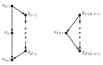
Figure 8.1. The $k$-midway property for the pair  $(\alpha_{s},\alpha_{s+r})$. The arrows point from smaller to larger poset elements.

Remark 8.12.

Figure 8.1 may seem surprising at first due to its vertical symmetry. So let us emphasize that in contrast with the $k$-pentagon property, the $k$-midway property is not invariant under poset duality due to the asymmetry of the labels. This is why it is different from the dual $k$-midway property even for posets of width two.

9. Final remarks and open problems

9.1.

Finding the equality conditions is an important problem for inequalities across mathematics, see e.g. [BB65], and throughout the sciences, see e.g. [Dahl96]. Notably, for geometric inequalities, such as the isoperimetric inequalities, these problems are classical (see e.g. [BZ88]), and in many cases the equality conditions are equally important and are substantially harder to prove. For example, in the Brunn–Minkowski inequality, the equality conditions are crucially used in the proof of the Minkowski theorem on existence of a polytope with given normals and facet volumes (see e.g. $\S$7.7, $\S$36.1 and $\S$41.6 in [Pak09]).

For poset inequalities, the equality conditions have also been studied, see e.g. an overview in [Win86]. In fact, Stanley’s original paper [Sta81] raises several versions of this question. In recent years, there were a number of key advances on combinatorial inequalities using algebraic and analytic tools, see e.g. [CP21, Huh18], but the corresponding equality conditions are understood in only very few instances.

9.2.

In a special case of the Kahn–Saks inequality, finding the equality conditions in full generality remains a major challenge. From this point of view, the equivalences  (a)  $\Rightarrow$  (b)  $\Rightarrow$  (c)  in Theorem 1.7 combined with Theorem 8.9 is the complete characterization in a special case of width two posets with two elements in the same chain. As we mentioned in the introduction, this result is optimal and does not extend even to elements in different chains.

We should also mention that both Stanley’s inequality (Theorem 1.1) and the equality conditions in Stanley’s inequality inequality (Theorem 8.1) was recently proved by elementary means in [CP21]. Despite our best efforts, the technology of [CP21] does not seem to translate to the Kahn–Saks inequality, suggesting the difference between the two. In fact, the close connection between the inequalities and equality conditions in the proofs of [CP21] hints that perhaps the equality conditions of the Kahn–Saks inequality are substantially harder to obtain.

9.3.

From the universe of poset inequalities, let us single out the celebrated XYZ inequality, which was later proved to be always strict [Fis84] (see also [Win86]). Another notable example in the Ahlswede–Daykin correlation inequality whose equality was studied in a series of papers, see [AK95] and references therein.

The Sidorenko inequality is an equality if and only if a poset is series–parallel, as proved in the original paper [Sid91]. The latter inequality turned out to be a special case of the conjectural Mahler inequality. It would be interesting to find an equality condition of the more general mixed Sidorenko inequality for pairs of two-dimensional posets, recently introduced in [AASS20].

In our previous paper [CPP21a], we proved both the cross–product inequality as well the equality conditions for the case of posets of width two. While in full generality this inequality implies the Kahn–Saks inequality, the reduction does not preserve the width of the posets, so the results in [CPP21a] do not imply the results in this paper. Let us also mention some recent work on poset inequalities for posets of width two [Chen18, Sah18] generalizing the classical approach in [Lin84].

9.4.

The bijection in Lemma 2.1, see also Remark 2.2, is natural from both order theory and enumerative combinatorics points of view. Indeed, the order ideals of a width two poset $P$ with fixed chain partitions  $(\mathcal{C}_{1},\mathcal{C}_{2})$  are in natural bijection with lattice points in a region  $\operatorname{\textnormal{Reg}}(P)\subset\mathbb{Z}^{2}$. Now the fundamental theorem for finite distributive lattices (see e.g. [Sta99, Thm 3.4.1]), gives the same bijection between  $\operatorname{\mathcal{E}}(P)$  and  lattice paths  $\operatorname{\mathbf{0}}\to(\emph{{a}},\emph{{b}})$  in  $\operatorname{\textnormal{Reg}}(P)$.

9.5.

As we mentioned in the introduction, the injective proof of the Stanley inequality (Theorem 1.3) given in Section 4, does in fact coincide with the CFG injection given in [CFG80]. The latter is stated somewhat informally, but we find the formalism useful for generalizations. In a different direction, our breakdown into lemmas allowed us a completely different generalization of the Stanley inequality to exit probabilities of random walks, which we discuss in a follow up paper [CPP21b].

9.6.

Maps  $\Phi,\Psi,\Omega,\Theta$  on  $\operatorname{\mathcal{E}}(P)$  used in the proofs of Theorem 8.5 and Theorem 8.9, are closely related to the promotion map heavily studied in poset literature, see e.g. [Sta99, $\S$3.20] and [Sta09]. We chose to avoid using the known properties of promotion to keep proofs simple and self-contained. Note that the promotion map can also be used to prove Proposition 8.3 as we do in greater generality in the forthcoming [CPP22+].

9.7.

Recall that computing  $e(P)$  is #P-complete even for posets of height two, or of dimension two; see [DP18] for an overview. The same holds for  $\textrm{N}(k)$, which both a refinement and a generalization of $\hskip 0.85355pte(P)$. Following the approach in [Pak09], it is natural to conjecture that  ${\text{\rm T}}(x,k)\hskip 1.70709pt:=\hskip 1.70709pt\textrm{N}(k)^{2}\hskip 0.85355pt-\hskip 0.85355pt\textrm{N}(k+1)\hskip 1.70709pt\textrm{N}(k-1)$  is #P-hard for general posets. We also conjecture that  ${\text{\rm T}}(x,k)$  is not in #P even though it is in  ${\textsc{GapP}}_{\geq 0}$  by definition. From this point of view, Corollary 8.4 is saying that the decision problem whether  ${\text{\rm T}}(x,k)=0$  is in P, further complicating the matter.

9.8.

There is an indirect way to derive both Corollaries 8.4 and 8.6 without explicit combinatorial conditions for vanishing of  $\textrm{N}(k)$  and $\textrm{F}(k)$, given in Proposition 8.3 and Theorem 8.5, respectively. In fact, the vanishing problem is in  P  by the following general result:

Theorem 9.1.

Let  $P=(X,\prec)$  be a finite poset with  $|X|=n$  elements, let  $x_{1}\ldots,x_{k}\in X$  be distinct poset elements, and let  $a_{1},\ldots,a_{k}\in\{1,\ldots,n\}$  be distinct integers. Finally, let  $\textrm{\em N}(a_{1},\ldots,a_{k})$  be the number of linear extensions  $L\in\operatorname{\mathcal{E}}(P)$  such that  $L(x_{i})=a_{i}$  for all  $1\leq i\leq i$. Then, deciding whether  $\textrm{\em N}(a_{1},\ldots,a_{k})=0$  can be done in  poly$(n)$  time.

Proof.

It was shown by Stanley [Sta81, Thm 3.2], that  $\textrm{N}(a_{1},\ldots,a_{k})/(n-k)!$  is equal to the mixed volume of certain polytopes $\hskip 0.85355ptK_{i}$  given by explicit combinatorial inequalities. In the terminology of [DGH98, p. 364], these polytopes $\hskip 0.85355ptK_{i}$  are well-presented, so by [DGH98, Thm 8] the vanishing of the mixed volume can be decided in polynomial time. ∎

To see the connection between the theorem and condition  $\textrm{F}(k)=0$, note that for every fixed  $x,y\in X$, we have  $\textrm{F}(k)=\textrm{N}(1,k+1)+\ldots+\textrm{N}(n-k,n)$. In the same way, the vanishing  $\textrm{F}(k,\ell)=0$  in the cross–product inequality (see [CPP21a]) can also be decided in polynomial time.

Note that the proof in [DGH98, Thm 8] involves a classical but technically involved matroid intersection algorithm by Edmonds (1970). Thus, finding an explicit combinatorial condition for vanishing of  $\textrm{N}(a_{1},\ldots,a_{k})$  is of independent interest.

Acknowledgements

We are grateful to Fedya Petrov, Ashwin Sah, Raman Sanyal, Yair Shenfeld and Ramon van Handel for helpful discussions on the subject, and to Leonid Gurvits for telling us about the [DGH98] reference. Special thanks to Ramon van Handel and Alan Yan for pointing out an important error in the previous version of the paper, and for suggesting Example 1.5. The last two authors were partially supported by the NSF.

References

- [AK95] R. Ahlswede and L. H. Khachatrian, Towards characterizing equality in correlation inequalities, European J. Combin. 16 (1995), 315–328.
- [AASS20] S. Artstein-Avidan, S. Sadovsky and R. Sanyal, Geometric inequalities for anti-blocking bodies, preprint (2020), 27 pp.; arXiv:2008.10394.
- [BB65] E. F. Beckenbach and R. Bellman, Inequalities (Second ed.), Springer, New York, 1965, 198 pp.
- [BZ88] Yu. D. Burago and V. A. Zalgaller, Geometric inequalities, Springer, Berlin, 1988, 331 pp.
- [CP21] S. H. Chan and I. Pak, Log-concave poset inequalities, preprint (2021), 71 pp.; arXiv:2110.10740.
-
[CPP21a]
S. H. Chan, I. Pak and G. Panova,
The cross–product conjecture for width two posets, preprint (2021), 30 pp.;
arXiv:2104.09009. -
[CPP21b]
S. H. Chan, I. Pak and G. Panova,
Log-concavity in planar random walks, preprint (2021), 8 pp.; arXiv:2106.
10640. - [CPP22+] S. H. Chan, I. Pak and G. Panova, Effective combinatorics of poset inequalities, in preparation (2022).
- [Chen18] E. Chen, A family of partially ordered sets with small balance constant, Electron. J. Combin. 25 (2018), Paper No. 4.43, 13 pp.
- [CFG80] F. R. K. Chung, P. C. Fishburn and R. L. Graham, On unimodality for linear extensions of partial orders, SIAM J. Algebraic Discrete Methods 1 (1980), 405–410.
- [Dahl96] R. A. Dahl, Equality versus inequality, Pol. Sci. and Pol. 29 (1996), 639–648.
- [DP18] S. Dittmer and I. Pak, Counting linear extensions of restricted posets, 33 pp.; arXiv:1802.06312.
- [DGH98] M. Dyer, P. Gritzmann and A. Hufnagel, On the complexity of computing mixed volumes, SIAM J. Comput. 27 (1998), 356–400.
- [Fis84] P. C. Fishburn, A correlational inequality for linear extensions of a poset, Order 1 (1984), 127–137.
- [GV89] I. M. Gessel and X. Viennot, Determinants, paths, and plane partitions, preprint (1989), 36 pp.; available at https://tinyurl.com/85z9v3m7
- [GJ83] I. P. Goulden and D. M. Jackson, Combinatorial enumeration, Wiley, New York, 1983, 569 pp.
- [GYY80] R. L. Graham, A. C. Yao and F. F. Yao, Some monotonicity properties of partial orders, SIAM J. Algebraic Discrete Methods 1 (1980), 251–258.
- [Huh18] J. Huh, Combinatorial applications of the Hodge–Riemann relations, in Proc. ICM Rio de Janeiro, Vol. IV, World Sci., Hackensack, NJ, 2018, 3093–3111.
- [KS84] J. Kahn and M. Saks, Balancing poset extensions, Order 1 (1984), 113–126.
- [Lin84] N. Linial, The information-theoretic bound is good for merging, SIAM J. Comput. 13 (1984), 795–801.
-
[Pak09]
I. Pak, Lectures on discrete and polyhedral geometry,
monograph draft (2009), 440 pp.; available at
http://www.math.ucla.edu/~pak/book.htm . - [Sah18] A. Sah, Improving the – conjecture for width two posets, Combinatorica 41 (2020), 99–126.
- [SvH20+] Y. Shenfeld and R. van Handel, The extremals of the Alexandrov–Fenchel inequality for convex polytopes, Acta Math., to appear, 82 pp.; arXiv:2011.04059.
- [Sid91] A. Sidorenko, Inequalities for the number of linear extensions, Order 8 (1991), 331–340.
- [Sta81] R. P. Stanley, Two combinatorial applications of the Aleksandrov–Fenchel inequalities, J. Combin. Theory, Ser. A 31 (1981), 56–65.
- [Sta99] R. P. Stanley, Enumerative Combinatorics, vol. 1 (second ed.) and vol. 2, Cambridge Univ. Press, 2012 and 1999.
- [Sta09] R. P. Stanley, Promotion and evacuation, Electron. J. Combin. 16 (2009), no. 2, Paper 9, 24 pp.
- [Win86] P. M. Winkler, Correlation and order, in Combinatorics and ordered sets, AMS, Providence, RI, 1986, 151–174.