On the Convergence of Differentially Private Federated Learning on Non-Lipschitz Objectives, and with Normalized Client Updates

Abstract

There is a dearth of convergence results for differentially private federated learning (FL) with non-Lipschitz objective functions (i.e., when gradient norms are not bounded). The primary reason for this is that the clipping operation (i.e., projection onto an $\ell_{2}$ ball of a fixed radius called the clipping threshold) for bounding the sensitivity of the average update to each client’s update introduces bias depending on the clipping threshold and the number of local steps in FL, and analyzing this is not easy. For Lipschitz functions, the Lipschitz constant serves as a trivial clipping threshold with zero bias. However, Lipschitzness does not hold in many practical settings; moreover, verifying it and computing the Lipschitz constant is hard. Thus, the choice of the clipping threshold is non-trivial and requires a lot of tuning in practice. In this paper, we provide the first convergence result for private FL on smooth convex objectives for a general clipping threshold – without assuming Lipschitzness. We also look at a simpler alternative to clipping (for bounding sensitivity) which is normalization – where we use only a scaled version of the unit vector along the client updates, completely discarding the magnitude information. The resulting normalization-based private FL algorithm is theoretically shown to have better convergence than its clipping-based counterpart on smooth convex functions. We corroborate our theory with synthetic experiments as well as experiments on benchmarking datasets.

1 Introduction

Collaborative machine learning (ML) schemes such as federated learning (FL) [MMR⁺17] are growing at an unprecedented rate. In contrast to the conventional centralized paradigm of training, wherein all the data is stored in a central database, FL (and in general, a collaborative ML scheme) enables training ML models from decentralized and heterogeneous data through collaboration of many participants, e.g., mobile devices, each with different data and capabilities. In a standard FL setting, there are $n$ clients (e.g., mobile phones or sensors), each with their own decentralized data, and a central server that is trying to train a model, parameterized by $\bm{w}\in\mathbb{R}^{d}$, using the clients’ data. Suppose the $i^{\text{th}}$ client has $m$ training examples/samples $\{\bm{x}_{1}^{(i)},\ldots,\bm{x}_{m}^{(i)}\}:=\mathcal{D}_{i}$, drawn from some distribution $\mathcal{P}_{i}$. Then the $i^{\text{th}}$ client has an objective function $f_{i}(\bm{w})$ which is the average loss, w.r.t. some loss function $\ell$, over its $m$ samples, and the central server tries to optimize the average loss $f(\bm{w})$, over the $n$ clients, i.e.,

$$f(\bm{w}):=\frac{1}{n}\sum_{i=1}^{n}{f_{i}}(\bm{w}),\text{ where }f_{i}(\bm{w}):=\frac{1}{m}\sum_{j=1}^{m}\ell(\bm{x}_{j}^{(i)},\bm{w}).$$ (1)

The setting where the data distributions of all the clients are identical, i.e. $\mathcal{P}_{1}=\ldots=\mathcal{P}_{n}$, is known as the “homogeneous” setting. Other settings are known as “heterogeneous” settings. We quantify heterogeneity in more detail in Section 2 (see Definition 1).

The key algorithmic idea of FL is Federated Averaging commonly abbreviated as FedAvg [MMR⁺17]. In FedAvg, at every round, the server randomly chooses a subset of the clients and sends them the latest global model. These clients then undertake multiple steps of local updates (on the global model received from the server) with their respective data based on (stochastic) gradient descent, and then communicate back their respective updated local models to the server. The server then averages the clients’ local models to update the global model (hence the name FedAvg). FedAvg forms the basis of more advanced federated optimization algorithms. For the sake of completeness, we state FedAvg in Algorithm 3 (Appendix A). The convergence of FedAvg as well as other FL algorithms depends heavily on the number of local updates as well as the degree of data heterogeneity – specifically, for the same number of local updates, the convergence worsens as the amount of heterogeneity increases.

Despite the locality of data storage in FL, information-sharing opens the door to the possibility of sabotaging the security of personal data through communication. Hence, it is crucial to devise effective, privacy-preserving communication strategies that ensure the integrity and confidentiality of user data. Differential privacy (DP) [DMNS06] is a popular privacy-quantifying framework that is being incorporated in the training of ML models. In particular, DP focuses on a learning algorithm’s sensitivity to an individual’s data; a less sensitive algorithm is less likely to leak individuals’ private details through its output. This idea has laid the foundation for designing a simple strategy to ensure privacy by adding random Gaussian or Laplacian noise to the output, where the noise is scaled according to the algorithm’s sensitivity to an individual’s data. We talk about DP in more detail in Section 2.

There has been a lot of work on differentially private optimization in order to enable private training of ML models. In this regard, DP-SGD [ACG⁺16] is the most widely used private optimization algorithm in the centralized setting. It is essentially the same as regular SGD, except that Gaussian noise is added to the average of the “clipped” per-sample gradients (or updates) for privacy. There is a natural extension of DP-SGD to the federated setting based on FedAvg, wherein the server receives a noise-perturbed average of the “clipped” client updates [GKN17, TAM19]; this is called DP-FedAvg (with clipping) and it is stated in Algorithm 1. Specifically, if the original update is $\bm{u}$, then its clipped version is $\bm{u}\min(1,\frac{C}{\|\bm{u}\|_{2}})$, for some threshold $C$; notice that this is the projection of $\bm{u}$ onto an $\ell_{2}$ ball of radius $C$ centered at the origin. Clipping is performed to bound the sensitivity of the average update to each individual update, which is required to set the variance of the added Gaussian noise; specifically, the noise variance is proportional to $C^{2}$.

While the privacy aspect of DP-SGD and its variants, both in the centralized and federated setting, is typically the main consideration, the optimization aspect – particularly due to clipping – is not given that much attention. Specifically, the average of the clipped updates is biased and the amount of bias depends on the clipping threshold $C$ – the higher the value of $C$, the lower is the bias, and vice-versa. But as mentioned before, the noise variance is proportional to $C^{2}$. Thus, the choice of the clipping threshold $C$ is associated with an intrinsic tension between the bias and variance of the noise-perturbed average of the clipped updates, which impacts the rate of convergence.

To provide convergence guarantees for DP-SGD, most prior works assume that the per-sample losses are Lipschitz (i.e., they have bounded gradients); under this assumption, setting $C$ equal to the Lipschitz constant results in zero bias, making the convergence analysis trivial. But in practice, we cannot ascertain the Lipschitzness property, let alone figuring out the Lipschitz constant, due to which the choice of the clipping threshold is not trivial and requires a lot of tuning. So ideally, we would like to have convergence results for non-Lipschitz functions. However, there aren’t too many in the literature, primarily because analyzing the clipping bias is not easy, and more so in the federated setting due to multiple local updates. A few works in the centralized setting do provide some results for the non-Lipschitz case by making more relaxed assumptions [CWH20, WXDX20, KLZ21, BWLS21]; we discuss these in Section 3. However, in the more challenging federated setting with multiple local update steps, there is no result even for the convex non-Lipschitz case. In this work, we provide the first convergence result for differentially private federated convex optimization with a general clipping threshold, while not assuming Lipschitzness or making any other relaxed assumption; see Theorems 2 and 3. Moreover, prior works do not consider whether performing multiple local update steps is indeed beneficial (or not) for private optimization; we make the first attempt to analyze this theoretically. Informally, under an extra assumption, our result indicates that multiple local update steps are beneficial if the degree of heterogeneity of the data is dominated by poor choice of initialization (of the model parameters) for training. See (c) in the discussion after Theorem 2.

Further, we also propose a simpler alternative (compared to clipping) for bounding the sensitivity which is to always normalize the individual client updates; specifically, if the original update is $\bm{u}$, then its normalized version is $\bm{u}(\frac{C}{\|\bm{u}\|_{2}})$, for some appropriate scaling factor $C$. Surprisingly, this simpler option has not been considered by prior works on private optimization. The resultant private FL algorithm, where we replace clipping by normalization, is summarized in Algorithm 2 and we call it DP-NormFedAvg. We explain why/how/when the simpler alternative of normalization will offer better convergence than clipping in private optimization both theoretically (see Section 5.1) as well as intuitively (see Section 5.2); we also elaborate on this while summarizing our contributions next.

Our main contributions are summarized next:
(a) In Theorem 2, we provide a convergence result for DP-FedAvg with clipping (Algorithm 1) which is the first convergence result for differentially private federated convex optimization with a general clipping threshold and without assuming Lipschitzness, followed by a simplified (but less tight) convergence result in Theorem 3. Based on our derived result, we also attempt to quantify the benefit/harm of performing multiple local update steps in private optimization. Informally, under an extra assumption (1), we show that multiple local updates are beneficial if the effect of poor initialization (of the model parameters) outweighs the effect of data heterogeneity by a factor depending on the privacy level; see (c) in the discussion after Theorem 2.

(b) In Section 5, we present DP-NormFedAvg (Algorithm 2) where we replace update clipping by the simpler alternative of update normalization (i.e., sending a scaled version of the unit vector along the update) for bounding the sensitivity. We provide a convergence result for DP-NormFedAvg in Theorem 4 and compare it against the result of DP-FedAvg with clipping (i.e., Theorem 2), showing that when the effect of poor initialization of the model parameters is more severe than the degree of data heterogeneity and/or if we can train for a large number of rounds, we expect the simpler alternative of normalization to offer better convergence than clipping in private optimization; see Remark 1 and Section 5.1 for details. Intuitively, this happens because normalization has a higher signal (i.e., update norm) to noise ratio than clipping; this aspect is discussed in detail in Section 5.2.

(c) We demonstrate the superiority of normalization over clipping via experiments on a synthetic quadratic problem in Section 5.3 as well as on three benchmarking datasets, viz., Fashion MNIST [XRV17], CIFAR-10 and CIFAR-100 in Section 6. For our synthetic experiment, we show that normalization has a higher signal to noise ratio than clipping (as mentioned above) in Figure 2, and that the trajectory of normalization (projected in 2D space) reaches closer to the optimum of the function than the trajectory of clipping in Figure 3. In the experiments on benchmarking datasets, for $\varepsilon=5$, the improvement offered by normalization over clipping w.r.t. the test accuracy is more than $2.8$% for CIFAR-100, $2.1$% for Fashion MNIST and $1.5$% for CIFAR-10; see Table 1.

2 Preliminaries

In this work, we are able to naturally quantify the effect of heterogeneity on convergence as follows.

Definition 1 (Heterogeneity).

Let $\bm{w}^{*}\in\arg\min_{\bm{w}^{\prime}\in\mathbb{R}^{d}}f(\bm{w}^{\prime})$ and $\Delta_{i}^{*}:=f_{i}(\bm{w}^{*})-\min_{\bm{w}^{\prime}\in\mathbb{R}^{d}}f_{i}(\bm{w}^{\prime})\geq 0$. Then the heterogeneity of the system is quantified by some increasing function of the $\Delta_{i}^{*}$’s.

The above way of quantifying heterogeneity shows up naturally in our convergence results for private FL assuming that the $f_{i}$’s are convex and smooth. The exact function of $\Delta_{i}^{*}$’s (quantifying heterogeneity) depends on the algorithm as well as data, and this will become clear when we present the convergence results. Also note that if the per-client data distributions (i.e, $\mathcal{P}_{i}$’s) are similar, then we expect the $\Delta_{i}^{*}$’s to be small indicating smaller heterogeneity.

Differential Privacy (DP): Suppose we have a collection of datasets ${D}_{c}$ and a query function $h:{D}_{c}\xrightarrow{}\mathcal{X}$. Two datasets $\mathcal{D}\in{D}_{c}$ and $\mathcal{D}^{\prime}\in{D}_{c}$ are said to be neighboring if they differ in exactly one sample, and we denote this by $|\mathcal{D}-\mathcal{D}^{\prime}|=1$. A randomized mechanism $\mathcal{M}:\mathcal{X}\xrightarrow{}\mathcal{Y}$ is said to be $(\varepsilon,\delta)$-DP, if for any two neighboring datasets $\mathcal{D},\mathcal{D}^{\prime}\in{D}_{c}$ and for any measurable subset of outputs $\mathcal{R}\in\mathcal{Y}$,

$$\mathbb{P}(\mathcal{M}(h(\mathcal{D}))\in\mathcal{R})\leq e^{\varepsilon}\mathbb{P}(\mathcal{M}(h(\mathcal{D}^{\prime}))\in\mathcal{R})+\delta.$$ (2)

When $\delta=0$, it is commonly known as pure DP. Otherwise, it is known as approximate DP.

Adding random Gaussian noise to the output of $h(.)$ above is the customary approach to provide DP; this is known as the Gaussian mechanism and we formally define it below.

Definition 2 (Gaussian mechanism [DR⁺14]).

Suppose $\mathcal{X}$ (i.e., the range of the query function $h$ above) is $\mathbb{R}^{p}$. Let $\Delta_{2}:=\sup_{\mathcal{D},\mathcal{D}^{\prime}\in{D}_{c}:|\mathcal{D}-\mathcal{D}^{\prime}|=1}\|h(\mathcal{D})-h(\mathcal{D}^{\prime})\|_{2}$. If we set

$$\mathcal{M}(h(\mathcal{D}))=h(\mathcal{D})+\bm{Z},$$

where $\bm{Z}\sim\mathcal{N}\Big{(}\vec{0}_{p},\frac{2\log(1.25/\delta)\Delta_{2}^{2}}{\varepsilon^{2}}\textup{I}_{p}\Big{)}$, then the mechanism $\mathcal{M}$ is $(\varepsilon,\delta)$-DP.

The Gaussian mechanism is also employed in private optimization [ACG⁺16].

Definition 3 (Lipschitz).

A function $g:\Theta\xrightarrow{}\mathbb{R}$ is to said to be $G$-Lipschitz if $\sup_{\bm{\theta}\in\Theta}\|\nabla g(\bm{\theta})\|_{2}\leq G$.

Definition 4 (Smoothness).

A function $g:\Theta\xrightarrow{}\mathbb{R}$ is to said to be $L$-smooth if for all $\bm{\theta},\bm{\theta}^{\prime}\in\Theta$, $\|\nabla g(\bm{\theta})-\nabla g(\bm{\theta}^{\prime})\|_{2}\leq L\|\bm{\theta}-\bm{\theta}^{\prime}\|_{2}$. If $g$ is twice differentiable, then for all $\bm{\theta},\bm{\theta}^{\prime}\in\Theta$:

$$g(\bm{\theta}^{\prime})\leq g(\bm{\theta})+\langle\nabla g(\bm{\theta}),\bm{\theta}^{\prime}-\bm{\theta}\rangle+\frac{L}{2}\|\bm{\theta}^{\prime}-\bm{\theta}\|_{2}^{2}.$$

Definition 5 (A Key Quantity).

All the theoretical results in this paper are expressed in terms of the following key quantity:

$$\rho:=\frac{\sqrt{qd\log({1}/{\delta})}}{n\varepsilon},$$ (3)

where $(\varepsilon,\delta)$-DP is the desired privacy level, $n$ is the number of samples, $d$ is the parameter dimension and $q$ is the absolute constant in Theorem 1. Further, all our results are for the non-vacuous privacy regime, i.e., when $\varepsilon$ is finite and $\delta<1$, where $\rho>0$. Finally, we also assume that $n$ is sufficiently large so that $\rho<1$.

Note that $\rho$ increases as the level of privacy increases (i.e., $\varepsilon$ and $\delta$ decrease), and vice versa.

Notation: Throughout the rest of this paper, we denote the $\ell_{2}$ norm simply by $\|.\|$ (omitting the subscript 2). Vectors and matrices are written in boldface. We denote the uniform distribution over the integers $\{0,\ldots,a\}$ (where $a\in\mathbb{N}$) by $\text{unif}[0,a]$. The function $\text{clip}:\mathbb{R}^{d}\times\mathbb{R}^{+}\xrightarrow{}\mathbb{R}^{d}$ is defined as:

$$\text{clip}(\bm{z},c):=\bm{z}\min\Big{(}1,\frac{c}{\|\bm{z}\|}\Big{)}.$$ (4)

$K$ is the number of communication rounds or the number of global updates, $E$ is the number of local updates per round, and $r$ is the number of clients that the server accesses in each round.

The proofs of all theoretical results are in the Appendix.

3 Related Work

Differentially private optimization: Most differentially private optimization algorithms for training ML models (both in the centralized and federated settings) are based off of DP-SGD, wherein the optimizer receives a Gaussian noise-perturbed average of the clipped per-sample gradients (to guarantee DP), and the moments accountant method [ACG⁺16]. Similar to and/or related to DP-SGD, there are several papers on private optimization algorithms in the centralized setting [CM08, CMS11, KST12, SCS13, DJW13, BST14, TGTZ15, WLK⁺17, ZZMW17, WYX18, INS⁺19, BFTT19, FKT20, AFKT21] as well as in the federated and distributed (without multiple local updates) setting [GKN17, ASY⁺18, TAM19, LLSS19, PKM19, NRY⁺21, GDD⁺21]. DP-FedAvg with clipping [GKN17, TAM19] (stated in Algorithm 1) is the most standard private algorithm in the federated setting. Among these previously mentioned works in the centralized setting, the ones that do provide convergence guarantees assume Lipschitzness and they set the clipping threshold equal to the Lipschitz constant, obtaining a suboptimality gap (i.e., $\mathbb{E}[f(\bm{w}_{\text{priv}})]-\min_{\bm{w}}f(\bm{w})$, where $\bm{w}_{\text{priv}}$ is the output) in the convex case of $\mathcal{O}(\rho)$, where $\rho=\mathcal{O}\Big{(}\frac{\sqrt{d\log({1}/{\delta})}}{n\varepsilon}\Big{)}$ is the key quantity defined in Definition 5. In fact, [BST14] show that in the convex Lipschitz case, the $\mathcal{O}(\rho)$ suboptimality gap is tight. However, as mentioned in Section 1, Lipschitzness is not a very practical assumption, due to which it is important to obtain convergence guarantees under weaker assumptions where there is no trivial clipping threshold. To that end, there a few results in the centralized setting that do not make the simplistic Lipschitzness assumption, but instead make more relaxed assumptions such as gradients having bounded moments [WXDX20, KLZ21] or the stochastic gradient noise having a symmetric probability distribution function [CWH20]. Also, [BWLS21] analyze full-batch DP-GD from the NTK perspective for deep learning models. In comparison, there are hardly any convergence results for private federated optimization (which is harder to analyze due to multiple local steps) of non-Lipschitz objectives; [ZCH⁺21] provide a complicated result for the nonconvex case, but surprisingly there is no result for the convex case. In addition, the role of multiple local steps in private FL has not been theoretically studied.

Normalized gradient descent (GD) and related methods: In the centralized setting, [HLSS15] propose (Stochastic) Normalized GD. This is based on a similar idea as DP-NormFedAvg – instead of using the (stochastic) gradient, use the unit vector along the (stochastic) gradient for the update. Extensions of this method incorporating momentum [YGG17, YLR⁺19, CM20] have been shown to significantly improve the training time of very large models such as BERT in the centralized setting. In the FL setting, [CGH⁺21] propose Normalized FedAvg, where the server uses a normalized version of the average of client updates (and not the average of normalized client updates, which is what we do) to improve training. However, it must be noted here that these works perform (some kind of) normalization to accelerate non-private training, whereas we are proposing normalization as an alternative sensitivity bounding mechanism to improve private training compared to the usual mechanism of clipping.

4 Convergence of Vanilla DP-FedAvg with Client-Update Clipping

First, we focus on the most standard version of DP-FedAvg involving client-update clipping, which is summarized in Algorithm 1. The primary difference from FedAvg is in lines 9, 10 and 12 of Algorithm 1. Each client in the selected subset of clients sends its clipped update plus zero-mean Gaussian noise (for differential privacy) to the server; since Gaussian noise is additive, we can add it at the clients itself. The server then computes the mean of the noisy clipped client updates that it received (i.e., $\bm{a}_{k}$) and then uses it to update the global model similar to FedAvg, except with a potentially different global learning rate ($\beta_{k}$) than the local learning rate ($\eta_{k}$). Since each $\bm{\zeta}^{(i)}_{k}$ (i.e., noise added at client $i$) is $\mathcal{N}(\vec{0}_{d},r\sigma^{2}\bm{\textup{I}}_{d})$, the average noise at the server is $\mathcal{N}(\vec{0}_{d},\sigma^{2}\bm{\textup{I}}_{d})$. Using the moments accountant method of [ACG⁺16], we now specify the value of $\sigma^{2}$ required to make Algorithm 1 $(\varepsilon,\delta)$-DP.

Theorem 1 ([ACG⁺16]).

For any $0<\varepsilon<\mathcal{O}\Big{(}\frac{r^{2}K}{n^{2}}\Big{)}$, Algorithm 1 will be $(\varepsilon,\delta)$-DP as long as

$$\sigma^{2}=qKC^{2}\frac{\log({1}/{\delta})}{n^{2}\varepsilon^{2}},$$ (5)

where $q>0$ is an absolute constant.

Note that the original DP-SGD algorithm of [ACG⁺16] returns the last iterate (i.e., $\bm{w}_{K}$) as the output, and Theorem 1 in their paper guarantees that the last iterate is $(\varepsilon,\delta)$-DP by setting $\sigma^{2}$ as per eq. 5. But if the last iterate is $(\varepsilon,\delta)$-DP, then so is any other iterate (due to additivity of the privacy cost), from which Theorem 1 follows.

Algorithm 1 DP-FedAvg (with clipping)

1:  Input: Initial point $\bm{w}_{0}$, number of rounds of communication $K$, number of local updates per round $E$, local learning rates $\{\eta_{k}\}_{k=0}^{K-1}$, global learning rates $\{\beta_{k}\}_{k=0}^{K-1}$, clipping threshold $C$, number of participating clients in each round $r$ and noise variance $\sigma^{2}$.

2:  for $k=0,\dots,K-1$ do

3:     Server sends $\bm{w}_{k}$ to a random set $\mathcal{S}_{k}$ of clients, formed by sampling each client $\in[n]$ with probability $r/n$.

4:     for client $i\in\mathcal{S}_{k}$ do

5:        Set $\bm{w}_{k,0}^{(i)}=\bm{w}_{k}$.

6:        for $\tau=0,\dots,E-1$ do

7:           Update $\bm{w}_{k,\tau+1}^{(i)}\xleftarrow{}\bm{w}_{k,\tau}^{(i)}-\eta_{k}\nabla f_{i}(\bm{w}_{k,\tau}^{(i)})$.

8:        end for

9:        Let $\bm{u}^{(i)}_{k}=\frac{\bm{w}_{k}-\bm{w}_{k,E}^{(i)}}{\eta_{k}}$ and $\bm{g}^{(i)}_{k}=\text{clip}\big{(}\bm{u}^{(i)}_{k},C\big{)}=\bm{u}^{(i)}_{k}\min\Big{(}1,\frac{C}{\|\bm{u}^{(i)}_{k}\|}\Big{)}$. // ($\bm{u}^{(i)}_{k}$ is client $i$’s update.)

10:        Send $(\bm{g}^{(i)}_{k}+\bm{\zeta}^{(i)}_{k})$ to the server, where $\bm{\zeta}^{(i)}_{k}\sim\mathcal{N}(\vec{0}_{d},r\sigma^{2}\bm{\textup{I}}_{d})$.

11:     end for

12:     Update $\bm{w}_{k+1}\xleftarrow{}\bm{w}_{k}-\beta_{k}\bm{a}_{k}$, where $\bm{a}_{k}=\frac{1}{r}\sum_{i\in\mathcal{S}_{k}}(\bm{g}^{(i)}_{k}+\bm{\zeta}^{(i)}_{k})$.

13:     Return $\bm{w}_{\text{priv}}=\bm{w}_{\tilde{k}}$, where $\tilde{k}\sim\text{unif}[0,K-1]$.

14:  end for

We now present the abridged convergence result for Algorithm 1; the full version and proof can be found in Appendix B.

Theorem 2 (Convergence of DP-FedAvg with Clipping: Convex Case).

Suppose each $f_{i}$ is convex and $L$-smooth over $\mathbb{R}^{d}$. Let $\hat{C}:=\frac{C}{E}$, where $C$ is the clipping threshold used in Algorithm 1. For any $\bm{w}^{*}\in\arg\min_{\bm{w}^{\prime}\in\mathbb{R}^{d}}f(\bm{w}^{\prime})$ and $\Delta_{i}^{*}:=f_{i}(\bm{w}^{*})-\min_{\bm{w}^{\prime}\in\mathbb{R}^{d}}f_{i}(\bm{w}^{\prime})\geq 0$, Algorithm 1 with $\hat{C}\geq 4\sqrt{L\max_{j\in[n]}\Delta_{j}^{*}}$, $\beta_{k}=\eta_{k}=\eta=\frac{\rho}{2\alpha L}$, $K=\big{(}\frac{2\alpha\gamma}{\hat{C}E}\big{)}\frac{1}{\rho^{2}}$ and $E\leq\frac{\alpha}{2\rho}$, where $\gamma>0$ and $\alpha\geq 1$ are constants of our choice, has the following convergence guarantee:

$$\mathbb{E}\Bigg{[}\frac{1}{n}\sum_{i=1}^{n}\Bigg{(}\mathbbm{1}(\|\bm{u}_{\tilde{k}}^{(i)}\|\leq\hat{C}E)\Big{(}2-\frac{\rho E}{\alpha}-\frac{\rho^{2}E^{2}}{\alpha^{2}}\Big{)}(f_{i}(\bm{w}_{\tilde{k}})-f_{i}(\bm{w}^{*}))+\mathbbm{1}(\|\bm{u}_{\tilde{k}}^{(i)}\|>\hat{C}E)\Big{(}\frac{3\hat{C}}{8LE}\|\bm{u}_{\tilde{k}}^{(i)}\|\Big{)}\Bigg{)}\Bigg{]}\\ \leq\underbrace{\hat{C}\Big{(}\frac{L\|\bm{w}_{0}-\bm{w}^{*}\|^{2}}{\gamma}+\frac{\gamma}{L}\Big{)}\rho}_{:=\textup{A(effect of {initialization})}}+\underbrace{\Big{(}\frac{3E}{2\alpha}\Big{)}\mathbb{E}\Bigg{[}\frac{1}{n}\sum_{i=1}^{n}{\mathbbm{1}(\|\bm{u}_{\tilde{k}}^{(i)}\|\leq\hat{C}E)}\Delta_{i}^{*}\Bigg{]}\rho}_{:=\textup{B(effect of {heterogeneity})}},$$ (6)

with $\tilde{k}\sim\textup{unif}[0,K-1]$.

In the above result, we remind the reader that $\bm{u}_{\tilde{k}}^{(i)}$ is the $i^{\text{th}}$ client’s update at a random round number $\tilde{k}$ (see line 9 in Algorithm 1). Also, this result is for the non-vacuous privacy regime, where $\rho:=\frac{\sqrt{qd\log({1}/{\delta})}}{n\varepsilon}>0$.

We also present a simplified, but less tight, convergence result based on Theorem 2; its proof is in Appendix C.

Theorem 3 (Simplified version of Theorem 2).

With $\gamma=\mathcal{O}(L\|\bm{w}_{0}-\bm{w}^{*}\|)$ and $\alpha=\mathcal{O}(1)$, the convergence result of Theorem 2 can be simplified to:

$$\mathbb{E}\Bigg{[}\frac{1}{n}\sum_{i=1}^{n}\min\Bigg{(}f_{i}(\bm{w}_{\tilde{k}})-f_{i}(\bm{w}^{*}),\mathcal{O}\Big{(}\frac{\hat{C}}{L}\|\nabla f_{i}(\bm{w}_{\tilde{k}})\|\Big{)}\Bigg{)}\Bigg{]}\leq\mathcal{O}\Bigg{(}\hat{C}\|\bm{w}_{0}-\bm{w}^{*}\|+E\Big{(}\frac{1}{n}\sum_{i=1}^{n}\Delta_{i}^{*}\Big{)}\Bigg{)}\rho.$$ (7)

We now delineate the key implications of Theorem 2.

(a) Convergence without assuming Lipschitzness: Note that Theorem 2 does not assume any $f_{i}$ to be Lipschitz. To our knowledge, this is the first convergence result for private federated convex optimization with a general clipping threshold, and without assuming Lipschitzness.

Let us also see what happens in the Lipschitz case. For that, suppose each $f_{i}$ is $G$-Lipschitz over $\mathbb{R}^{d}$. So if we set $\hat{C}=G$, then $\|\bm{u}_{k}^{(i)}\|\leq\hat{C}E$ for all $k$. Now, using the fact that $(2-\frac{\rho E}{\alpha}-\frac{\rho^{2}E^{2}}{\alpha^{2}})\geq\frac{5}{4}$ for $E\leq\frac{\alpha}{2\rho}$, the convergence result in Theorem 2 (i.e., eq. 6) reduces to:

$$\mathbb{E}[f(\bm{w}_{\tilde{k}})]-f(\bm{w}^{*})\leq\frac{4}{5}\Bigg{(}G\Big{(}\frac{L\|\bm{w}_{0}-\bm{w}^{*}\|^{2}}{\gamma}+\frac{\gamma}{L}\Big{)}+\frac{3E}{2\alpha}\Big{(}\frac{1}{n}\sum_{i=1}^{n}\Delta_{i}^{*}\Big{)}\Bigg{)}\rho.$$ (8)

Thus with $E=\mathcal{O}(1)$, our bound matches the lower bound of [BST14] for the centralized convex and Lipschitz case with respect to the dependence on $\rho$.

(b) Effect of initialization and heterogeneity: Observe that our convergence result depends on two things: (i) term A in eq. 6, i.e. the distance of the initialization $\bm{w}_{0}$ from the optimum $\bm{w}^{*}$, and (ii) term B in eq. 6, i.e. the degree of heterogeneity which itself depends on the $\Delta_{i}^{*}$’s (as per Definition 1). A high (respectively, low) degree of heterogeneity implies high (respectively, low) values of $\Delta_{i}^{*}$’s, which leads to worse (respectively, better) convergence. Also, as we increase $\alpha$ in Theorem 2, i.e. increase the number of rounds $K$, the effect of the heterogeneity term (B) dies down. However, the effect of the initialization term (A) cannot be diminished by increasing $\alpha$.

(c) Effect of multiple local steps: Characterizing whether having multiple local steps, i.e. $E>1$, is beneficial or detrimental is not obvious from Theorem 2. The RHS of eq. 6 seems to suggest that the convergence result gets worse as we increase $E$ – but this is whilst keeping $\hat{C}$ fixed. The intricacy here is that for the “same amount of clipping”, the required value of $\hat{C}$ is a non-increasing function of $E$. To make this more precise, let us consider two values of $E$, say $E_{1}$ and $E_{2}$ where $E_{1}<E_{2}$. Suppose the corresponding clipping thresholds that we use are $C_{1}=\hat{C}_{1}E_{1}$ and $C_{2}=\hat{C}_{2}E_{2}$, respectively. Now if we wish to have $\mathbbm{1}(\|\bm{u}_{\tilde{k}}^{(i)}\|\leq\hat{C}_{1}E_{1})=\mathbbm{1}(\|\bm{u}_{\tilde{k}}^{(i)}\|\leq\hat{C}_{2}E_{2})$, i.e. the “same amount of clipping” with $E_{1}$ and $E_{2}$, then $\hat{C_{2}}\leq\hat{C_{1}}$. This is because we are doing gradient descent on convex functions locally, due to which $\frac{\big{\|}\bm{u}_{\tilde{k}}^{(i)}\big{\|}}{E}=\frac{\big{\|}\sum_{\tau=0}^{E-1}\nabla f_{i}(\bm{w}_{\tilde{k},\tau}^{(i)})\big{\|}}{E}$ is a non-increasing function of $E$. However, quantifying the extent of “non-increasingness” of ${\|\bm{u}_{\tilde{k}}^{(i)}\|}/{E}$ – which allows us to provide choices of $\hat{C}$ as a function of $E$ – is not easy (and perhaps not possible) without making more assumptions other than convexity and smoothness. So, we now make a couple of extra assumptions (one of which is the standard Lipschitzness assumption) in 1, which then allows us to illustrate and quantify the “non-increasingness” of $\hat{C}$ as a function of $E$ in Proposition 1.

Assumption 1.

(i) For any $\bm{w}\in\mathbb{R}^{d}$ and each $i\in[n]$, we have that:

$$\|\nabla f_{i}(\bm{w}-\eta\nabla f_{i}(\bm{w}))-\nabla f_{i}(\bm{w})\|\geq\eta\lambda\|\nabla f_{i}(\bm{w})\|,$$ (9)

for some $0<\lambda\leq L$ and $\eta\leq\frac{\rho}{2L}$.

(ii) Additionally, each $f_{i}$ is $G$-Lipschitz over $\mathbb{R}^{d}$.

1 (i) can be also interpreted as a lower bound on the norm of the product of the Hessian matrix and the gradient vector. This is because for small enough $\eta$, we have:

$$\|\nabla f_{i}(\bm{w}-\eta\nabla f_{i}(\bm{w}))-\nabla f_{i}(\bm{w})\|=\Theta(\eta\|\nabla^{2}f_{i}(\bm{w})\nabla f_{i}(\bm{w})\|).$$ (10)

So basically for 1 (i) to hold, we are assuming $\|\nabla^{2}f_{i}(\bm{w})\nabla f_{i}(\bm{w})\|\geq\Omega(\lambda\|\nabla f_{i}(\bm{w})\|)$; note that a similar assumption has been made in [DKLH18]. Also, 1 (i) is a weaker assumption than strong convexity. This is because strong convexity would imply that $\|\nabla^{2}f_{i}(\bm{w})\bm{v}\|\geq\mu\|\bm{v}\|$ for any $\bm{v}\in\mathbb{R}^{d}$ and some $\mu>0$, while we assume this to hold only for $\bm{v}=\nabla f_{i}(\bm{w})$ (with $\mu=\Omega(\lambda)$). color=red!25, inline]Rudrajit: Can we improve the convergence of DP-FedAvg (i.e., either the dependence on $\rho$ or $K/E$) with this assumption? – Probably NOT

Proposition 1 ($\hat{C}$ under 1).

Set $\alpha=1$ in Theorem 2; this imposes the constraint $E\leq\frac{1}{2\rho}$. Then, under 1, choosing $\hat{C}=G\Big{(}1-\frac{11(E-1){\rho}}{64}\big{(}\frac{\lambda^{2}}{L^{2}}\big{)}\Big{)}$ in Theorem 2 ensures that $\mathbbm{1}(\|\bm{u}_{{k}}^{(i)}\|>\hat{C}E)=0$ $\forall$ $k$, i.e. no clipping happens for all $E$.

The proof of Proposition 1 is in Appendix D. Notice that $\hat{C}$, which is set so that the same (= zero) amount of clipping happens for all $E$ ($\leq\frac{1}{2\rho}$), is a non-increasing (more specifically, a decreasing) function of $E$ as mentioned before. It is worth mentioning here that the value of $\hat{C}$ in Proposition 1 is not the tightest possible value, but even for the tightest value, the non-increasingness will hold.

To summarize, there is a tradeoff involved as far as the number of local steps $E$ is concerned. Increasing $E$ allows us to reduce $\hat{C}$ which mitigates the effect of initialization, i.e. term A in eq. 6, but at the cost of increasing the effect of heterogeneity, i.e. term B in eq. 6. To illustrate this tradeoff, let us plug in our choice of $\hat{C}$ derived in Proposition 1 in the convergence result of Theorem 2 with $\gamma=L\|\bm{w}_{0}-\bm{w}^{*}\|$ (this choice is just for simplicity). After a bit of simplification, this yields:

$$\mathbb{E}[f(\bm{w}_{\tilde{k}})]-f(\bm{w}^{*})\leq\Bigg{(}2G{\|\bm{w}_{0}-\bm{w}^{*}\|}+\frac{6E}{5}\Bigg{\{}\frac{1}{n}\sum_{i=1}^{n}\Delta_{i}^{*}-\frac{11G\|\bm{w}_{0}-\bm{w}^{*}\|\rho}{48}\Big{(}\frac{\lambda^{2}}{L^{2}}\Big{)}\Bigg{\}}\Bigg{)}\rho.$$ (11)

Equation 11 tells us that if $\frac{1}{n}\sum_{i=1}^{n}\Delta_{i}^{*}<\mathcal{O}\Big{(}{G}\big{(}\frac{\lambda^{2}}{L^{2}}\big{)}\Big{)}\|\bm{w}_{0}-\bm{w}^{*}\|\rho$, which in plain English basically means that if the degree of heterogeneity is less than the product of the distance of the initialization from the optimum and $\rho=\mathcal{O}\Big{(}\frac{\sqrt{d\log(1/\delta)}}{n\varepsilon}\Big{)}$ (and some other data-dependent constants), then having a large value of $E$ is beneficial; in particular, setting the maximum permissible value of $E$, which is $\frac{1}{2\rho}$, is the best (in terms of smallest suboptimality gap). Otherwise, having a small value of $E$ is better; specifically, setting $E=1$ is the best. From Theorem 2, recall that for $\alpha=1$, $K=\Big{(}\frac{2\gamma}{\hat{C}E}\Big{)}\frac{1}{\rho^{2}}$; so the higher we set $E$, the fewer the number of communication rounds needed.

From the above discussion, one should not form the opinion that a poor initialization, i.e., a $\bm{w}_{0}$ such that $\|\bm{w}_{0}-\bm{w}^{*}\|$ is large, is advantageous in private FL. This is because choosing such a $\bm{w}_{0}$ will increase the first term within the big round brackets in eq. 11, i.e. $2G{\|\bm{w}_{0}-\bm{w}^{*}\|}$, which happens to be the dominant term – leading to a high suboptimality gap by default.

color=red!25, inline]Rudrajit: MORE CHANGES NEEDED ABOVE? If initialization is poor, anyways final error is gonna be bad…probably mention this.

5 DP-NormFedAvg: DP-FedAvg with Client-Update Normalization (instead of Clipping)

We define the normalization function $\text{norm}:\mathbb{R}^{d}-\{\vec{0}_{d}\}\times\mathbb{R}^{+}\xrightarrow{}\mathbb{R}^{d}$ as:

$$\text{norm}(\bm{z},c):=\frac{c\bm{z}}{\|\bm{z}\|},$$ (12)

where $c$ is the scaling factor. The parameter $c$ is analogous to the clipping threshold in the $\text{clip}(.)$ function. Also, note that $\|\text{norm}(\bm{z},c)\|\leq c$ holds.

Here we propose to normalize client-updates instead of clipping them, i.e., we propose to change line 9 of Algorithm 1 as follows:

$$\bm{g}^{(i)}_{k}=\text{norm}(\bm{u}_{k}^{(i)},C).$$ (13)

We call the resultant algorithm DP-NormFedAvg because it involves normalizing updates in DP-FedAvg. For completeness, we state it in Algorithm 2; note the normalization step in line 9.

Algorithm 2 DP-NormFedAvg

1:  Input: Initial point $\bm{w}_{0}$, number of rounds of communication $K$, number of local updates per round $E$, local learning rates $\{\eta_{k}\}_{k=0}^{K-1}$, global learning rates $\{\beta_{k}\}_{k=0}^{K-1}$, scaling factor $C$, number of participating clients in each round $r$ and noise variance $\sigma^{2}$.

2:  for $k=0,\dots,K-1$ do

3:     Server sends $\bm{w}_{k}$ to a random set $\mathcal{S}_{k}$ of clients, formed by sampling each client $\in[n]$ with probability $r/n$.

4:     for client $i\in\mathcal{S}_{k}$ do

5:        Set $\bm{w}_{k,0}^{(i)}=\bm{w}_{k}$.

6:        for $\tau=0,\dots,E-1$ do

7:           Update $\bm{w}_{k,\tau+1}^{(i)}\xleftarrow{}\bm{w}_{k,\tau}^{(i)}-\eta_{k}\nabla f_{i}(\bm{w}_{k,\tau}^{(i)})$.

8:        end for

9:        Let $\bm{u}^{(i)}_{k}=\frac{\bm{w}_{k}-\bm{w}_{k,E}^{(i)}}{\eta_{k}}$ and $\bm{g}^{(i)}_{k}=\text{norm}\big{(}\bm{u}^{(i)}_{k},C\big{)}=\frac{C\bm{u}^{(i)}_{k}}{\|\bm{u}^{(i)}_{k}\|}$. // (Normalization instead of Clipping.)

10:        Send $(\bm{g}^{(i)}_{k}+\bm{\zeta}^{(i)}_{k})$ to the server, where $\bm{\zeta}^{(i)}_{k}\sim\mathcal{N}(\vec{0}_{d},r\sigma^{2}\bm{\textup{I}}_{d})$.

11:     end for

12:     Update $\bm{w}_{k+1}\xleftarrow{}\bm{w}_{k}-\beta_{k}\bm{a}_{k}$, where $\bm{a}_{k}=\frac{1}{r}\sum_{i\in\mathcal{S}_{k}}(\bm{g}^{(i)}_{k}+\bm{\zeta}^{(i)}_{k})$.

13:     Return $\bm{w}_{\text{priv}}=\bm{w}_{\tilde{k}}$, where $\tilde{k}\sim\text{unif}[0,K-1]$.

14:  end for

The abridged convergence result of DP-NormFedAvg is presented next. The full version and proof can be found in Appendix E.

Theorem 4 (Convergence of DP-NormFedAvg: Convex Case).

In the same setting and with the same choices as Theorem 2, DP-NormFedAvg (i.e., Algorithm 2) has the following convergence guarantee:

$$\mathbb{E}\Bigg{[}\frac{1}{n}\sum_{i=1}^{n}\Bigg{\{}\mathbbm{1}(\|\bm{u}_{\tilde{k}}^{(i)}\|\leq\hat{C}E)\Big{(}2-\frac{\rho^{2}E^{2}}{\alpha^{2}}\Big{)}\Bigg{(}\frac{\hat{C}E}{\|\bm{u}_{\tilde{k}}^{(i)}\|}\Bigg{)}(f_{i}(\bm{w}_{\tilde{k}})-f_{i}(\bm{w}^{*}))+\mathbbm{1}(\|\bm{u}_{\tilde{k}}^{(i)}\|>\hat{C}E)\Big{(}\frac{3\hat{C}\|\bm{u}_{\tilde{k}}^{(i)}\|}{8LE}\Big{)}\Bigg{\}}\Bigg{]}\\ \leq\hat{C}\Big{(}\frac{L\|\bm{w}_{0}-\bm{w}^{*}\|^{2}}{\gamma}+\frac{\gamma}{L}\Big{)}\rho+{\mathbb{E}\Bigg{[}\frac{1}{n}\sum_{i=1}^{n}\mathbbm{1}(\|\bm{u}_{\tilde{k}}^{(i)}\|\leq\hat{C}E)\Bigg{\{}\frac{\hat{C}^{2}}{2\alpha L}+\Bigg{(}\frac{\hat{C}E}{\|\bm{u}_{\tilde{k}}^{(i)}\|}\Bigg{)}\frac{\Delta_{i}^{*}\rho E}{\alpha^{2}}\Bigg{\}}E\Bigg{]}}\rho,$$ (14)

with $\tilde{k}\sim\textup{unif}[0,K-1]$.

We now provide some insights on the convergence rate of Theorem 4 by comparing it with that of DP-FedAvg with clipping (i.e., Theorem 2).

5.1 Theoretical Comparison of DP-FedAvg with Clipping and DP-NormFedAvg

Per Theorem 2, recall that the convergence rate of DP-FedAvg with clipping (i.e., Algorithm 1) is:

$$\mathbb{E}\Bigg{[}\frac{1}{n}\sum_{i=1}^{n}\Bigg{(}\mathbbm{1}(\|\bm{u}_{\tilde{k}}^{(i)}\|\leq\hat{C}E){\color[rgb]{0,1,1}\Big{(}2-\frac{\rho E}{\alpha}-\frac{\rho^{2}E^{2}}{\alpha^{2}}\Big{)}}(f_{i}(\bm{w}_{\tilde{k}})-f_{i}(\bm{w}^{*}))+\mathbbm{1}(\|\bm{u}_{\tilde{k}}^{(i)}\|>\hat{C}E)\Big{(}\frac{3\hat{C}}{8LE}\|\bm{u}_{\tilde{k}}^{(i)}\|\Big{)}\Bigg{)}\Bigg{]}\\ \leq\underbrace{\hat{C}\Big{(}\frac{L\|\bm{w}_{0}-\bm{w}^{*}\|^{2}}{\gamma}+\frac{\gamma}{L}\Big{)}\rho}_{:=\textup{A}\text{(effect of {initialization})}}+\underbrace{{\color[rgb]{0,1,1}\mathbb{E}\Bigg{[}\frac{1}{n}\sum_{i=1}^{n}{\mathbbm{1}(\|\bm{u}_{\tilde{k}}^{(i)}\|\leq\hat{C}E)}\Big{(}\frac{3E}{2\alpha}\Big{)}\Bigg{]}}\rho}_{:=\textup{B}\text{(effect of {heterogeneity})}},$$ (15)

with $\tilde{k}\sim\textup{unif}[0,K-1]$. In comparison, the convergence rate of DP-NormFedAvg (i.e., Algorithm 2), under the same setting, is:

$$\mathbb{E}\Bigg{[}\frac{1}{n}\sum_{i=1}^{n}\Bigg{\{}\mathbbm{1}(\|\bm{u}_{\tilde{k}}^{(i)}\|\leq\hat{C}E)\underbrace{\color[rgb]{1,0,0}\Big{(}2-\frac{\rho^{2}E^{2}}{\alpha^{2}}\Big{)}}_{>(2-\frac{\rho E}{\alpha}-\frac{\rho^{2}E^{2}}{\alpha^{2}})}\underbrace{\color[rgb]{1,0,0}\Bigg{(}\frac{\hat{C}E}{\|\bm{u}_{\tilde{k}}^{(i)}\|}\Bigg{)}}_{\geq 1}(f_{i}(\bm{w}_{\tilde{k}})-f_{i}(\bm{w}^{*}))+\mathbbm{1}(\|\bm{u}_{\tilde{k}}^{(i)}\|>\hat{C}E)\Big{(}\frac{3\hat{C}}{8LE}\|\bm{u}_{\tilde{k}}^{(i)}\|\Big{)}\Bigg{\}}\Bigg{]}\\ \leq\underbrace{\hat{C}\Big{(}\frac{L\|\bm{w}_{0}-\bm{w}^{*}\|^{2}}{\gamma}+\frac{\gamma}{L}\Big{)}\rho}_{=\textup{A}\text{(effect of {initialization})}}+\underbrace{{\color[rgb]{1,0,0}\mathbb{E}\Bigg{[}\frac{1}{n}\sum_{i=1}^{n}\mathbbm{1}(\|\bm{u}_{\tilde{k}}^{(i)}\|\leq\hat{C}E)\Bigg{\{}\frac{\hat{C}^{2}}{2\alpha L}+\Bigg{(}\frac{\hat{C}E}{\|\bm{u}_{\tilde{k}}^{(i)}\|}\Bigg{)}\frac{\Delta_{i}^{*}\rho E}{\alpha^{2}}\Bigg{\}}E\Bigg{]}}\rho}_{:=\textup{B}_{2}\text{(effect of {heterogeneity})}}.$$ (16)

The terms that are different in eq. 15 and eq. 16 have been colored. Let us consider the same choice of $\hat{C}$ and optimum $\bm{w}^{*}$ for both algorithms. As discussed earlier, the convergence rate depends on: (i) distance of the initialization $\bm{w}_{0}$ from the optimum $\bm{w}^{*}$ (specifically, term A in both equations), and (ii) the degree of heterogeneity which is itself a function of the $\Delta_{i}^{*}$’s (specifically, term B and $\textup{B}_{2}$ in eq. 15 and eq. 16, respectively).

Note that the LHS of eq. 16 is larger than the LHS of eq. 15. Thus, the effect of term A, i.e. the effect of initialization, on convergence is smaller in the case of normalization than clipping. Next, recalling that we must set $\hat{C}\geq 4\sqrt{L\max_{j\in[n]}\Delta_{j}^{*}}$ in both Theorem 2 and 4, let us choose $\hat{C}=c\sqrt{L\max_{j\in[n]}\Delta_{j}^{*}}$ with $c\geq 4$ in both cases. Then:

$$\textup{B}_{2}={\mathbb{E}\Bigg{[}\frac{1}{n}\sum_{i=1}^{n}\mathbbm{1}(\|\bm{u}_{\tilde{k}}^{(i)}\|\leq\hat{C}E)\Bigg{\{}\Bigg{(}\frac{c^{2}E}{2\alpha}\Bigg{)}\max_{j\in[n]}\Delta_{j}^{*}+\Bigg{(}\frac{\hat{C}E}{\|\bm{u}_{\tilde{k}}^{(i)}\|}\Bigg{)}\Bigg{(}\frac{\Delta_{i}^{*}\rho E^{2}}{\alpha^{2}}\Bigg{)}\Bigg{\}}\Bigg{]}}\rho.$$ (17)

Now observe that for $c\geq 4$, $\textup{B}<\textup{B}_{2}$. However, the LHS of eq. 16 is more than that of eq. 15. So in general, it is difficult to predict whether the effect of heterogeneity on convergence is smaller in the case of clipping or normalization.

But the effect of heterogeneity can be mitigated arbitrarily for both clipping and normalization by increasing $\alpha$, i.e. increasing the number of rounds $K$ arbitrarily (recall that we set $K=\big{(}\frac{2\alpha\gamma}{\hat{C}E}\big{)}\frac{1}{\rho^{2}}$). So asymptotically, i.e. for $\alpha\to\infty$ or $K\to\infty$, the effect of heterogeneity gets killed and only the effect of initialization matters, where we expect normalization to outperform clipping. It is worth mentioning here that the previous discussion is not specific to the federated setting and also applies to the centralized setting (i.e., $E=1$).

We summarize all the above discussion in the following remark.

Remark 1 (Normalization versus Clipping).

Compared to clipping, normalization is associated with a smaller effect of initialization on convergence. However, in general, it is difficult to characterize whether the effect of heterogeneity is smaller for normalization or clipping. The good thing is that for both clipping and normalization, the effect of heterogeneity gets killed asymptotically, i.e. when the number of communication rounds ($K$) tends to $\infty$.

Hence, for problems that do not have a high degree of heterogeneity and the effect of initialization is more severe (for e.g., by poor random initialization) and/or if we can train for a very large number of rounds, we expect normalization to offer better convergence than clipping in private optimization.

It is also worth pointing out that clipping can be equivalent to normalization in certain scenarios. Specifically, suppose the client update norms are lower bounded by ${C}_{\text{low}}$; then, clipping with threshold $C\leq{C}_{\text{low}}$ is equivalent to normalization with the same scaling factor.

In Section 5.2, we provide a more intuitive argument as to why update normalization can offer better convergence than update clipping in terms of their signal (viz., update norm) to noise ratios, and also relate it to the previous theoretical comparison in Section 5.1.

5.2 Intuitive Explanation of why Normalization can Outperform Clipping

Intuitively, clipping has the following issue with respect to optimization - as the client update norms decrease and fall below the clipping threshold, the norm of the added noise (which has constant expectation proportional to the clipping threshold, regardless of the client update norms) can become arbitrarily larger than the client update norms, which should inhibit convergence. This issue is not as grave in DP-NormFedAvg because its update-normalization step ensures that the noise norm cannot become arbitrarily larger than the normalized update’s norm (even if the original update’s norm is small). In other words, the signal (which is the update norm) to noise ratio of clipping eventually falls below that of normalization.

The mathematical manifestation of the aforementioned argument can be also seen in the convergence bounds of clipping (i.e., eq. 15) and normalization (i.e., eq. 16) in Section 5.1. Specifically, note that the coefficient of $\mathbbm{1}(\|\bm{u}_{\tilde{k}}^{(i)}\|\leq\hat{C}E)$ (i.e., when the update norm $\|\bm{u}_{\tilde{k}}^{(i)}\|$ is less than or equal to the clipping threshold $\hat{C}E$) in the LHS of eq. 16 is at least $\frac{\hat{C}E}{\|\bm{u}_{\tilde{k}}^{(i)}\|}$ ($\geq 1$) times more than the corresponding term in the LHS of eq. 15; this amplification is a consequence of the improvement in signal to noise ratio (SNR) of normalization over clipping. On the other hand, the coefficient of $\mathbbm{1}(\|\bm{u}_{\tilde{k}}^{(i)}\|>\hat{C}E)$ (i.e., when the update norm is more than the clipping threshold) in the LHS of eq. 16 is exactly the same as the corresponding term in the LHS of eq. 15; this is because normalization and clipping are equivalent when $\|\bm{u}_{\tilde{k}}^{(i)}\|>\hat{C}E$. Now, as discussed in Section 5.1, the RHS of both eq. 15 and eq. 16 become the same asymptotically with a large number of rounds as the effect of heterogeneity dies down. Thus, the asymptotic convergence of normalization (i.e., eq. 16) is better than that of clipping (i.e., eq. 15). color=red!25, inline]Rudrajit: Try to improve and shorten the above rationale?

Let us now see some experimental results on a synthetic problem illustrating the superiority of normalization over clipping.

5.3 Empirical Comparison of DP-FedAvg with Clipping and DP-NormFedAvg on a Synthetic Problem

We consider $f_{i}(\bm{w})=\frac{1}{2}(\bm{w}-\bm{w}_{i}^{*})^{T}\bm{Q}_{i}(\bm{w}-\bm{w}_{i}^{*})$, where $i\in[100]$ (so, $n=100$) and $\bm{w}\in\mathbb{R}^{200}$ (so, $d=200$). Further, $\bm{w}_{i}^{*}$ is drawn i.i.d. from $\mathcal{N}(0,\textup{I}_{200})$ and $\bm{Q}_{i}=\bm{A}_{i}\bm{A}_{i}^{T}$, where $\bm{A}_{i}$ is a $200\times 20$ matrix whose entries are drawn i.i.d from $\mathcal{N}(0,\frac{1}{20^{2}})$; hence, $\bm{Q}_{i}$ is a PSD matrix with bounded maximum eigenvalue, due to which $f_{i}$ is convex and smooth.

We set $(\varepsilon,\delta)=(5,10^{-6})$, $K=500$ and $E=20$ for this set of experiments. We consider two different initializations with different distances from the global optimum $\bm{w}^{*}$:

• I1: $\bm{w}_{0}=\bm{w}^{*}+\bm{z}$, and

• I2: $\bm{w}_{0}=\bm{w}^{*}+\frac{\bm{z}}{5}$,

where each coordinate of $\bm{z}$ is drawn i.i.d. from the continuous uniform distribution with support (0,1). We set $\eta_{k}=\beta_{k}=\eta$ for all rounds $k$, and also have full-device participation. In Figure 1, we plot the function suboptimality (i.e., $f(\bm{w}_{k})-f(\bm{w}^{*})$ at round number $k$) of DP-FedAvg with Clipping and DP-NormFedAvg for different values of $\eta$ and clipping threshold/scaling factor $C$, for I1 and I2; specifically, “Clip($\eta$)” and “Norm($\eta$)” in the legend denote DP-FedAvg with Clipping and DP-NormFedAvg with $\eta_{k}=\beta_{k}=\eta$ for all rounds $k$, respectively. In Figure 2, for each round $k$, we plot the corresponding $\text{SNR}:=\frac{\big{\|}\frac{1}{r}\sum_{i\in\mathcal{S}_{k}}\bm{g}^{(i)}_{k}\big{\|}}{\big{\|}\frac{1}{r}\sum_{i\in\mathcal{S}_{k}}\bm{\zeta}^{(i)}_{k}\big{\|}}$, where $\bm{g}^{(i)}_{k}$ and $\bm{\zeta}^{(i)}_{k}$ are the clipped/normalized per-client update and per-client noise, respectively, as defined in Algorithm 1/2. We only show the SNR plots for one value of $\eta$ as the trend for other values of $\eta$ is similar (and to avoid congestion). All plots are averaged over three independent runs. For a fair comparison, in each run, the exact same noise vectors (sampled randomly at each round) are used in both algorithms.

The thing to note in Figure 1 is that for $C=\{50,100\}$ and all values of $\eta$, normalization attains an appreciably lower function suboptimality than clipping. For $C=40$, normalization is just slightly better. The SNR values in Figure 2 also follow a similar trend – the improvement in SNR for normalization compared to clipping is much higher for $C=\{50,100\}$ than $C=40$. We only show results up to $C=40$ as for smaller values of $C$, clipping and normalization are equivalent. As discussed at the end of Section 5.1 after Remark 1, recall that if the client update norms are lower bounded by ${C}_{\text{low}}$, then clipping with threshold $C\leq{C}_{\text{low}}$ is equivalent to normalization with the same scaling factor.

For further illustration, in Figure 3, we plot the smoothed 2D projection of the trajectories of DP-FedAvg with clipping and DP-NormFedAvg for two of the cases of Figure 1. From here, we can see that DP-NormFedAvg reaches closer to the optimum than DP-FedAvg with clipping. color=red!25, inline]Rudrajit: Add details about how these trajectories are generated? Also remember to change the caption of Figure 3 should anything change.

These plots corroborate our previous theoretical predictions and intuition. We also show the superiority of normalization over clipping via experiments on actual datasets in Section 6.

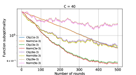
(a)

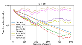
(b)

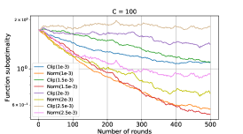
(c)

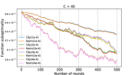
(d)

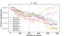
(e)

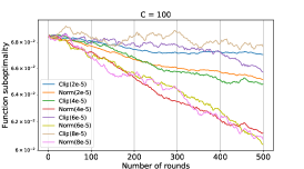
(f)

Figure 1: Function suboptimality (i.e., $f(\bm{w}_{k})-f(\bm{w}^{*})$ at round number $k$) of DP-FedAvg with Clipping and DP-NormFedAvg for different values of $\eta$ (recall, $\eta_{k}=\beta_{k}=\eta$ for all rounds $k$) and clipping threshold/scaling factor $C$, for I1 and I2 described in Section 5.3. Specifically, “Clip($\eta$)” and “Norm($\eta$)” denote DP-FedAvg with Clipping and DP-NormFedAvg with $\eta_{k}=\beta_{k}=\eta$, respectively. All plots are averaged over three independent runs.
For $C=\{50,100\}$ and all values of $\eta$, normalization does significantly better than clipping. For $C=40$ (and lower), normalization and clipping are nearly equivalent, but clipping never does better than normalization. This validates our theoretical predictions in Section 5.1.

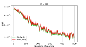
(a)

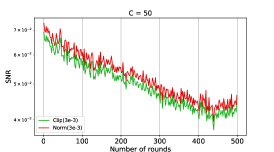
(b)

(c)

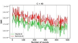
(d)

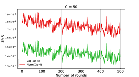
(e)

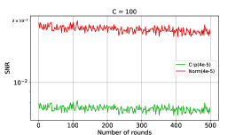
(f)

Figure 2: In the same setting and with the same notation as Figure 1, comparison of $\text{SNR}:=\frac{\big{\|}\frac{1}{r}\sum_{i\in\mathcal{S}_{k}}\bm{g}^{(i)}_{k}\big{\|}}{\big{\|}\frac{1}{r}\sum_{i\in\mathcal{S}_{k}}\bm{\zeta}^{(i)}_{k}\big{\|}}$, where $\bm{g}^{(i)}_{k}$ and $\bm{\zeta}^{(i)}_{k}$ are the clipped/normalized per-client update and per-client noise, as defined in Algorithm 1/2. The SNR for only one value of $\eta$ is shown here as the trend for other values of $\eta$ is similar.
As per our discussion in Section 5.2, the SNR of normalization is never lower than that of clipping, explaining the superiority of the former.

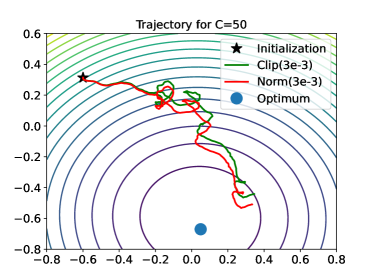
(a)

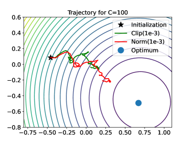
(b)

Figure 3: Smoothed 2D projections of the trajectories of DP-FedAvg with clipping and DP-NormFedAvg for two of the cases considered in Figure 1. Observe that DP-NormFedAvg reaches closer to the optimum than DP-FedAvg with clipping.

6 Experiments

We consider the task of private multi-class classification to compare DP-FedAvg with clipping against DP-NormFedAvg; for brevity, we will often call them just clipping and normalization, respectively. Our experiments are performed on three benchmarking datasets, Fashion-MNIST [XRV17] (abbreviated as FMNIST henceforth), CIFAR-10 and CIFAR-100, where the first two datasets have $10$ classes each and the last one has $100$ classes.

Specifically, we consider logistic regression on FMNIST, CIFAR-10 and CIFAR-100 with $\ell_{2}$-regularization; the weight decay value in PyTorch for $\ell_{2}$-regularization is set to 1e-4. For FMNIST, we flatten each image into a $784$-dimensional vector and use that as the feature vector. For CIFAR-10 and CIFAR-100, we use 512-dimensional features extracted from the last layer of a ResNet-18 [HZRS16] model pretrained on ImageNet. Similar to [MMR⁺17], we simulate a heterogeneous setting by distributing the data among the clients such that each client can have data from at most five classes. The exact procedure is described in Appendix G. For the CIFAR-10 and CIFAR-100 (respectively, FMNIST) experiment, the number of clients $n$ is set to 5000 (respectively, 3000), with each client having the same number of samples. The number of participating clients in each round is set to $r=0.2n$ for all datasets, with 20 local client updates per-round.

We consider two privacy levels: $\varepsilon=\{5,1.5\}$ with $\delta=10^{-5}$; note that $\varepsilon=5$ (respectively, $1.5$) corresponds to the low (respectively, high) privacy regime. For clipping and normalization, the values of $C$ that we tune over are $\{500,250,125,62.5,31.25,15.625\}$. The details about the learning rate schedule can be found in Appendix G. In Table 1, we show the comparison between clipping and normalization (in terms of test accuracy) for the two aforementioned privacy levels as well as vanilla FedAvg (without any privacy) as the baseline. The results reported here are the best ones for each algorithm by tuning over $C$ and the learning rates, and have been averaged over three different runs.

In all cases, normalization is clearly superior to clipping. It is worth noting that the improvement obtained with normalization is more for the low privacy regime (i.e., $\varepsilon=5$). color=red!25, inline]Rudrajit: More comments and experiments?

Algo.	$(5,10^{-5})$-DP	$(1.5,10^{-5})$-DP
Clipping	75.59%	56.90%
Normalization	77.72%	57.80%
FedAvg (w/o privacy)	83.43%

(a) FMNIST

Algo.	$(5,10^{-5})$-DP	$(1.5,10^{-5})$-DP
Clipping	82.63%	81.53%
Normalization	84.21%	82.42%
FedAvg (w/o privacy)	85.64%

(b) CIFAR-10

Algo.	$(5,10^{-5})$-DP	$(1.5,10^{-5})$-DP
Clipping	56.53%	41.33%
Normalization	59.36%	42.76%
FedAvg (w/o privacy)	64.61%

(c) CIFAR-100

Table 1: Average test accuracy over the last 5 rounds for (a) FMNIST, (b) CIFAR-10 and (c) CIFAR-100. Recall that “Clipping” and “Normalization” denote DP-FedAvg with Clipping and DP-NormFedAvg, respectively. The accuracy of FedAvg, which is our baseline without privacy, is at the bottom.

7 Conclusion

In this work, we provide the first convergence result for DP-FedAvg with clipping (which is the most standard algorithm for differentially private FL) in the convex case, and without assuming Lipschitzness. We also propose DP-NormFedAvg which normalizes client updates rather than clipping them (which is the customary approach for bounding sensitivity). Theoretically, we argue that DP-NormFedAvg should have better convergence than DP-FedAvg with clipping for problems that do not have a high degree of heterogeneity and the effect of poor initialization is more severe, and/or if we can train for a large number of rounds. Intuitively, this happens because normalization has a higher signal (i.e., update norm) to noise ratio than clipping. We also show the superiority of normalization over clipping via several experiments.

Several avenues of future work are possible. One of them is to provide principled recommendations on how to set the clipping threshold. Another one is to explore the feasibility of using adaptive and/or round-dependent clipping thresholds. It would be also nice to come up with meaningful additional assumptions that hold in practice, in order to simplify and/or improve our convergence results.

8 Acknowledgement

This work is supported in part by NSF grants CCF-1564000, IIS-1546452 and HDR-1934932.

Appendix A The FedAvg Algorithm

For the sake of completeness, here we state the famous FedAvg algorithm of [MMR⁺17] (with local updates using full gradients).

Algorithm 3 FedAvg [MMR⁺17]

1:  Input: Initial point $\bm{w}_{0}$, number of rounds of communication $K$, number of local updates per round $E$, local learning rates $\{\eta_{k}\}_{k=0}^{K-1}$ and number of participating clients in each round $r$.

2:  for $k=0,\dots,K-1$ do

3:     Server sends $\bm{w}_{k}$ to a random set $\mathcal{S}_{k}$ of $r$ clients chosen uniformly at random.

4:     for client $i\in\mathcal{S}_{k}$ do

5:        Set $\bm{w}_{k,0}^{(i)}=\bm{w}_{k}$.

6:        for $\tau=0,\ldots,E-1$ do

7:           Update $\bm{w}_{k,\tau+1}^{(i)}\xleftarrow{}\bm{w}_{k,\tau}^{(i)}-\eta_{k}\nabla f_{i}(\bm{w}_{k,\tau}^{(i)})$.

8:        end for

9:        Send $\bm{w}_{k}-\bm{w}_{k,E}^{(i)}$ to the server.

10:     end for

11:     Update $\bm{w}_{k+1}\xleftarrow{}\bm{w}_{k}-\frac{1}{r}\sum_{i\in\mathcal{S}_{k}}(\bm{w}_{k}-\bm{w}_{k,E}^{(i)})$. // (The above is equivalent to $\bm{w}_{k+1}\xleftarrow{}\frac{1}{r}\sum_{i\in\mathcal{S}_{k}}\bm{w}_{k,E}^{(i)}$, so the clients might as well just send the $\bm{w}_{k,E}^{(i)}$’s.)

12:  end for

Appendix B Full Version of Theorem 2 and its Proof

Theorem 5 (Full version of Theorem 2).

Suppose each $f_{i}$ is convex and $L$-smooth over $\mathbb{R}^{d}$. Let $\hat{C}:=\frac{C}{E}$, where $C$ is the clipping threshold used in Algorithm 1. For any $\bm{w}^{*}\in\arg\min_{\bm{w}^{\prime}\in\mathbb{R}^{d}}f(\bm{w}^{\prime})$ and $\Delta_{i}^{*}:=f_{i}(\bm{w}^{*})-\min_{\bm{w}^{\prime}\in\mathbb{R}^{d}}f_{i}(\bm{w}^{\prime})\geq 0$, Algorithm 1 with $\hat{C}\geq 4\sqrt{L\max_{j\in[n]}\Delta_{j}^{*}}$, $\beta_{k}=\eta_{k}=\eta=\big{(}\frac{\gamma}{\hat{C}LEK}\big{)}\frac{1}{\rho}$ and $K>\big{(}\frac{2\gamma}{\hat{C}E}\big{)}\frac{1}{\rho}$, where $\gamma>0$ is a constant of our choice, has the following convergence guarantee:

$$\mathbb{E}\Bigg{[}\frac{1}{n}\sum_{i=1}^{n}\Bigg{(}\mathbbm{1}(\|\bm{u}_{\tilde{k}}^{(i)}\|\leq\hat{C}E)\Big{(}2-\frac{2\gamma}{\hat{C}K\rho}-\frac{4\gamma^{2}}{\hat{C}^{2}K^{2}{\rho^{2}}}\Big{)}(f_{i}(\bm{w}_{\tilde{k}})-f_{i}(\bm{w}^{*}))+\mathbbm{1}(\|\bm{u}_{\tilde{k}}^{(i)}\|>\hat{C}E)\Big{(}\frac{3\hat{C}\|\bm{u}_{\tilde{k}}^{(i)}\|}{8LE}\Big{)}\Bigg{)}\Bigg{]}\\ \leq\hat{C}\Big{(}\frac{L\|\bm{w}_{0}-\bm{w}^{*}\|^{2}}{\gamma}+\frac{\gamma}{L}\Big{)}\rho+\Bigg{(}\frac{2\gamma}{\hat{C}K\rho}\Bigg{)}\Bigg{(}1+\frac{2\gamma}{\hat{C}K\rho}\Bigg{)}\mathbb{E}\Bigg{[}\frac{1}{n}\sum_{i=1}^{n}{\mathbbm{1}(\|\bm{u}_{\tilde{k}}^{(i)}\|\leq\hat{C}E)}\Delta_{i}^{*}\Bigg{]},$$

with $\tilde{k}\sim\textup{unif}[0,K-1]$.
Specifically, with $K=\big{(}\frac{2\alpha\gamma}{\hat{C}E}\big{)}\frac{1}{\rho^{2}}$ and $E\leq\frac{\alpha}{2\rho}$, where $\alpha\geq 1$ is another constant of our choice, Algorithm 1 has the following convergence guarantee:

$$\mathbb{E}\Bigg{[}\frac{1}{n}\sum_{i=1}^{n}\Bigg{(}\mathbbm{1}(\|\bm{u}_{\tilde{k}}^{(i)}\|\leq\hat{C}E)\Big{(}2-\frac{\rho E}{\alpha}-\frac{\rho^{2}E^{2}}{\alpha^{2}}\Big{)}(f_{i}(\bm{w}_{\tilde{k}})-f_{i}(\bm{w}^{*}))+\mathbbm{1}(\|\bm{u}_{\tilde{k}}^{(i)}\|>\hat{C}E)\Big{(}\frac{3\hat{C}\|\bm{u}_{\tilde{k}}^{(i)}\|}{8LE}\Big{)}\Bigg{)}\Bigg{]}\\ \leq\hat{C}\Big{(}\frac{L\|\bm{w}_{0}-\bm{w}^{*}\|^{2}}{\gamma}+\frac{\gamma}{L}\Big{)}\rho+\Big{(}\frac{3E}{2\alpha}\Big{)}\mathbb{E}\Bigg{[}\frac{1}{n}\sum_{i=1}^{n}{\mathbbm{1}(\|\bm{u}_{\tilde{k}}^{(i)}\|\leq\hat{C}E)}\Delta_{i}^{*}\Bigg{]}\rho.$$

B.1 Proof of Theorem 5:

Proof.

Let us set $\eta_{k}=\beta_{k}=\eta$ for all $k\geq 0$.

The update rule of the global iterate is:

$$\bm{w}_{k+1}=\bm{w}_{k}-\eta\Big{(}\frac{1}{r}\sum_{i\in\mathcal{S}_{k}}\text{clip}\big{(}\bm{u}_{k}^{(i)},C\big{)}+\bm{\zeta}_{k}\Big{)},$$ (18)

where $\bm{\zeta}_{k}=\frac{1}{r}\sum_{i\in\mathcal{S}_{k}}\bm{\zeta}^{(i)}_{k}\sim\mathcal{N}(\vec{0}_{d},\frac{qK\log(1/\delta)C^{2}}{n^{2}\varepsilon^{2}}\bm{\textup{I}}_{d})$ and

$$\bm{u}_{k}^{(i)}=\frac{(\bm{w}_{k}-\bm{w}_{k,E}^{(i)})}{\eta}=\sum_{\tau=0}^{E-1}\nabla f_{i}(\bm{w}_{k,\tau}^{(i)}).$$ (19)

Taking expectation with respect to the randomness in the current round, we get for any $\bm{w}^{*}\in\arg\min_{\bm{w}^{\prime}\in\mathbb{R}^{d}}f(\bm{w}^{\prime})$:

$$\mathbb{E}[\|\bm{w}_{k+1}-\bm{w}^{*}\|^{2}] =\mathbb{E}\Big{[}\Big{\|}\bm{w}_{k}-\eta\Big{(}\frac{1}{r}\sum_{i\in\mathcal{S}_{k}}\text{clip}(\bm{u}_{k}^{(i)},C)+\bm{\zeta}_{k}\Big{)}-\bm{w}^{*}\Big{\|}^{2}\Big{]}$$ (20)

$$=\|\bm{w}_{k}-\bm{w}^{*}\|^{2}-2\eta\mathbb{E}_{\mathcal{S}_{k}}\Big{[}\frac{1}{r}\sum_{i\in\mathcal{S}_{k}}\langle\text{clip}(\bm{u}_{k}^{(i)},C),\bm{w}_{k}-\bm{w}^{*}\rangle\Big{]}+\eta^{2}\mathbb{E}\Big{[}\Big{\|}\frac{1}{r}\sum_{i\in\mathcal{S}_{k}}\text{clip}(\bm{u}_{k}^{(i)},C)+\bm{\zeta}_{k}\Big{\|}^{2}\Big{]}$$ (21)

$$=\|\bm{w}_{k}-\bm{w}^{*}\|^{2}+\frac{1}{n}\sum_{i=1}^{n}{-2\eta\langle\text{clip}(\bm{u}_{k}^{(i)},C),\bm{w}_{k}-\bm{w}^{*}\rangle}+\eta^{2}\mathbb{E}_{\mathcal{S}_{k}}\Big{[}\Big{\|}\frac{1}{r}\sum_{i\in\mathcal{S}_{k}}\text{clip}(\bm{u}_{k}^{(i)},C)\Big{\|}^{2}\Big{]}$$ (22)

$$\hskip 28.45274pt+\eta^{2}\Big{(}\frac{qKd\log(1/\delta)C^{2}}{n^{2}\varepsilon^{2}}\Big{)}$$

$$\leq\|\bm{w}_{k}-\bm{w}^{*}\|^{2}+\frac{1}{n}\sum_{i=1}^{n}{-2\eta\langle\text{clip}(\bm{u}_{k}^{(i)},C),\bm{w}_{k}-\bm{w}^{*}\rangle}+\eta^{2}\mathbb{E}_{\mathcal{S}_{k}}\Big{[}\frac{1}{r}\sum_{i\in\mathcal{S}_{k}}\big{\|}\text{clip}(\bm{u}_{k}^{(i)},C)\big{\|}^{2}\Big{]}$$ (23)

$$\hskip 28.45274pt+\eta^{2}\Big{(}\frac{qKd\log(1/\delta)C^{2}}{n^{2}\varepsilon^{2}}\Big{)}$$

$$=\|\bm{w}_{k}-\bm{w}^{*}\|^{2}+\frac{1}{n}\sum_{i=1}^{n}\Big{\{}\underbrace{-2\eta\langle\text{clip}(\bm{u}_{k}^{(i)},C),\bm{w}_{k}-\bm{w}^{*}\rangle+\eta^{2}\big{\|}\text{clip}(\bm{u}_{k}^{(i)},C)\big{\|}^{2}}_{A_{i}}\Big{\}}$$ (24)

$$\hskip 28.45274pt+\eta^{2}\Big{(}\frac{qKd\log(1/\delta)C^{2}}{n^{2}\varepsilon^{2}}\Big{)}.$$

Note that eq. 23 is obtained by using 2. Let us examine $A_{i}$ for each $i$.

Case 1: $\|\bm{u}_{k}^{(i)}\|>C$. So we have $\text{clip}(\bm{u}_{k}^{(i)},C)=\frac{C}{\|\bm{u}_{k}^{(i)}\|}\bm{u}_{k}^{(i)}$. Thus,

$$A_{i} ={-2\eta C}{\Big{\langle}\frac{\bm{u}_{k}^{(i)}}{\|\bm{u}_{k}^{(i)}\|},\bm{w}_{k}-\bm{w}^{*}\Big{\rangle}}+\eta^{2}C^{2}$$ (25)

$$=\frac{-C}{\big{\|}\bm{u}_{k}^{(i)}\big{\|}}\Big{(}\|\bm{w}_{k}-\bm{w}^{*}\|^{2}+\eta^{2}\big{\|}\bm{u}_{k}^{(i)}\big{\|}^{2}-\|\underbrace{\bm{w}_{k}-\eta\bm{u}_{k}^{(i)}}_{=\bm{w}_{k,E}^{(i)}}-\bm{w}^{*}\|^{2}\Big{)}+\eta^{2}C^{2},$$ (26)

where the last step follows by using the fact for any two vectors $\bm{a}$ and $\bm{b}$, $\langle\bm{a},\bm{b}\rangle=\frac{1}{2}\Big{(}\|\bm{a}\|^{2}+\|\bm{b}\|^{2}-\|\bm{a}-\bm{b}\|^{2})$. Next, notice that $\bm{w}_{k}-\eta\bm{u}_{k}^{(i)}=\bm{w}_{k,E}^{(i)}$. Since $f_{i}$ is convex, we use Lemma 1 to get:

$$\|\bm{w}_{k}-\bm{w}^{*}\|^{2}-\|\bm{w}_{k,E}^{(i)}-\bm{w}^{*}\|^{2}\geq\frac{\eta}{2L}\sum_{\tau=0}^{E-1}\|\nabla f_{i}(\bm{w}_{k,\tau}^{(i)})\|^{2}-2\eta E\Delta_{i}^{*},$$ (27)

for $\eta\leq\frac{1}{2L}$ with $\Delta_{i}^{*}:=f_{i}(\bm{w}^{*})-\min_{\bm{w}^{\prime}\in\mathbb{R}^{d}}f_{i}(\bm{w}^{\prime})\geq 0$. But:

$$\big{\|}\bm{u}_{k}^{(i)}\big{\|}^{2} =\big{\|}\sum_{\tau=0}^{E-1}\nabla f_{i}(\bm{w}_{k,\tau}^{(i)})\big{\|}^{2}\leq E\sum_{\tau=0}^{E-1}\big{\|}\nabla f_{i}(\bm{w}_{k,\tau}^{(i)})\big{\|}^{2}.$$ (28)

The inequality above follows from 2. Using this in eq. 27, we get:

$$\|\bm{w}_{k}-\bm{w}^{*}\|^{2}-\|\bm{w}_{k,E}^{(i)}-\bm{w}^{*}\|^{2}\geq\frac{\eta}{2LE}\big{\|}\bm{u}_{k}^{(i)}\big{\|}^{2}-2\eta E\Delta_{i}^{*}.$$ (29)

Plugging this back in eq. 26, we get:

$$A_{i}\leq-C\Big{(}\eta^{2}+\frac{\eta}{2LE}\Big{)}{\|\bm{u}_{k}^{(i)}\|}+2\eta\underbrace{\Bigg{(}\frac{C}{\|\bm{u}_{k}^{(i)}\|}\Bigg{)}}_{<1}E\Delta_{i}^{*}+\eta^{2}C^{2},$$ (30)

for $\eta\leq\frac{1}{2L}$.

Let us choose $C^{2}\geq 16LE^{2}\max_{j\in[n]}\Delta_{j}^{*}$. Then, we have $E\Delta_{i}^{*}\leq\frac{C^{2}}{16LE}\leq\frac{C\|\bm{u}_{k}^{(i)}\|}{16LE}$. Using this in eq. 30, we get:

$$A_{i} \leq-C\Big{(}\eta^{2}+\frac{\eta}{2LE}\Big{)}\|\bm{u}_{k}^{(i)}\|+\frac{\eta C}{8LE}\|\bm{u}_{k}^{(i)}\|+\eta^{2}C^{2}$$ (31)

$$=-\frac{3\eta C}{8LE}\|\bm{u}_{k}^{(i)}\|+\eta^{2}C\underbrace{(C-\|\bm{u}_{k}^{(i)}\|)}_{<0}$$ (32)

$$\leq-\frac{3\eta C}{8LE}\|\bm{u}_{k}^{(i)}\|,$$ (33)

for $C\geq 4E\sqrt{L\max_{j\in[n]}\Delta_{j}^{*}}$ and $\eta\leq\frac{1}{2L}$.

Case 2: $\|\bm{u}_{k}^{(i)}\|\leq C$. So we have $\text{clip}(\bm{u}_{k}^{(i)},C)=\bm{u}_{k}^{(i)}$. Thus,

$$A_{i} ={-2\eta}{\langle\bm{u}_{k}^{(i)},\bm{w}_{k}-\bm{w}^{*}\rangle}+\eta^{2}\|\bm{u}_{k}^{(i)}\|^{2}\leq{-2\eta}\underbrace{\langle\bm{u}_{k}^{(i)},\bm{w}_{k}-\bm{w}^{*}\rangle}_{B_{i}}+2\eta^{2}LE^{2}(f_{i}(\bm{w}_{k})-f_{i}^{*}),$$ (34)

for $\eta L\leq{1}$; the inequality $\|\bm{u}_{{k}}^{(i)}\|^{2}\leq 2LE^{2}(f_{i}(\bm{w}_{k})-f_{i}^{*})$ (for $\eta L\leq{1}$) is obtained from Lemma 2. Now:

$$B_{i} =\langle\bm{u}_{k}^{(i)},\bm{w}_{k}-\bm{w}^{*}\rangle$$ (35)

$$=\sum_{\tau=0}^{E-1}\langle\nabla f_{i}(\bm{w}_{k,\tau}^{(i)}),\bm{w}_{k}-\bm{w}^{*}\rangle$$ (36)

$$=\sum_{\tau=0}^{E-1}\{\langle\nabla f_{i}(\bm{w}_{k,\tau}^{(i)}),\bm{w}_{k,\tau}^{(i)}-\bm{w}^{*}\rangle+\langle\nabla f_{i}(\bm{w}_{k,\tau}^{(i)}),\bm{w}_{k}-\bm{w}_{k,\tau}^{(i)}\rangle\}$$ (37)

$$\geq\sum_{\tau=0}^{E-1}\{f_{i}(\bm{w}_{k,\tau}^{(i)})-f_{i}(\bm{w}^{*})+\langle\nabla f_{i}(\bm{w}_{k}),\bm{w}_{k}-\bm{w}_{k,\tau}^{(i)}\rangle+\langle\nabla f_{i}(\bm{w}_{k,\tau}^{(i)})-\nabla f_{i}(\bm{w}_{k}),\bm{w}_{k}-\bm{w}_{k,\tau}^{(i)}\rangle\}$$ (38)

$$\geq\sum_{\tau=0}^{E-1}\{f_{i}(\bm{w}_{k,\tau}^{(i)})-f_{i}(\bm{w}^{*})+f_{i}(\bm{w}_{k})-f_{i}(\bm{w}_{k,\tau}^{(i)})-L\|\bm{w}_{k}-\bm{w}_{k,\tau}^{(i)}\|^{2}\}$$ (39)

$$=E(f_{i}(\bm{w}_{k})-f_{i}(\bm{w}^{*}))-L\sum_{\tau=0}^{E-1}\|\bm{w}_{k}-\bm{w}_{k,\tau}^{(i)}\|^{2}.$$ (40)

Note that eq. 38 follows from the convexity of $f_{i}$, while eq. 39 follows by once again using the convexity of $f_{i}$, the smoothness of $f_{i}$ as well as the Cauchy-Schwarz inequality.
Again, from Lemma 2, we have

$$\|\bm{w}_{k}-\bm{w}_{k,\tau}^{(i)}\|^{2}\leq 2\eta^{2}L\tau^{2}(f_{i}(\bm{w}_{k})-f_{i}^{*}),$$ (41)

for $\eta L\leq 1$. Using eq. 41 in eq. 40, we get

$$B_{i}\geq E(f_{i}(\bm{w}_{k})-f_{i}(\bm{w}^{*}))-2\eta^{2}L^{2}\sum_{\tau=0}^{E-1}\tau^{2}(f_{i}(\bm{w}_{k})-f_{i}^{*})\geq E(f_{i}(\bm{w}_{k})-f_{i}(\bm{w}^{*}))-2\eta^{2}L^{2}E^{3}(f_{i}(\bm{w}_{k})-f_{i}^{*}).$$ (42)

Now using eq. 42 in eq. 34, we get

$$A_{i} \leq-2\eta E(f_{i}(\bm{w}_{k})-f_{i}(\bm{w}^{*}))+4\eta^{3}L^{2}E^{3}(f_{i}(\bm{w}_{k})-f_{i}^{*})+2\eta^{2}LE^{2}(f_{i}(\bm{w}_{k})-f_{i}^{*})$$

$$=-\eta E{\Big{(}2-2\eta LE-4\eta^{2}L^{2}E^{2}\Big{)}}(f_{i}(\bm{w}_{k})-f_{i}(\bm{w}^{*}))+(2\eta^{2}LE^{2}+4\eta^{3}L^{2}E^{3})\Delta_{i}^{*},$$ (43)

for $\eta\leq\frac{1}{L}$.

Combining the results of Case 1 and 2, i.e. eq. 33 and eq. 43, we get

$$A_{i}\leq\mathbbm{1}(\|\bm{u}_{k}^{(i)}\|>C)\Big{(}-\frac{3\eta C}{8LE}\|\bm{u}_{k}^{(i)}\|\Big{)}\\ +\mathbbm{1}(\|\bm{u}_{k}^{(i)}\|\leq C)\Big{(}-{\eta E}(2-2\eta LE-4\eta^{2}L^{2}E^{2})(f_{i}(\bm{w}_{k})-f_{i}(\bm{w}^{*}))+(2\eta^{2}LE^{2}+4\eta^{3}L^{2}E^{3})\Delta_{i}^{*}\Big{)},$$ (44)

for $C\geq 4E\sqrt{L\max_{j\in[n]}\Delta_{j}^{*}}$ and $\eta\leq\frac{1}{2L}$. Let us define $\hat{C}:=\frac{C}{E}$. Then eq. 44 can be re-written as:

$$A_{i}\leq-{\eta E}\Bigg{\{}\mathbbm{1}(\|\bm{u}_{k}^{(i)}\|\leq\hat{C}E)\Big{(}(2-2\eta LE-4\eta^{2}L^{2}E^{2})(f_{i}(\bm{w}_{k})-f_{i}(\bm{w}^{*}))\Big{)}\\ +{\mathbbm{1}(\|\bm{u}_{k}^{(i)}\|>\hat{C}E)\Big{(}\frac{3\hat{C}}{8LE}\|\bm{u}_{k}^{(i)}\|\Big{)}}-\mathbbm{1}(\|\bm{u}_{k}^{(i)}\|\leq\hat{C}E)(2\eta LE+4\eta^{2}L^{2}E^{2})\Delta_{i}^{*}\Bigg{\}},$$ (45)

where $\hat{C}\geq 4\sqrt{L\max_{j\in[n]}\Delta_{j}^{*}}$ and $\eta\leq\frac{1}{2L}$. Now using eq. 45 in eq. 24, we get:

$$\mathbb{E}[\|\bm{w}_{k+1}-\bm{w}^{*}\|^{2}]\leq\|\bm{w}_{k}-\bm{w}^{*}\|^{2}-\frac{\eta E}{n}\sum_{i=1}^{n}\Big{\{}\mathbbm{1}(\|\bm{u}_{{k}}^{(i)}\|>\hat{C}E)\Big{(}\frac{3\hat{C}}{8LE}\|\bm{u}_{k}^{(i)}\|\Big{)}\\ +\mathbbm{1}(\|\bm{u}_{{k}}^{(i)}\|\leq\hat{C}E)\Big{(}(2-2\eta LE-4\eta^{2}L^{2}E^{2})(f_{i}(\bm{w}_{{k}})-f_{i}(\bm{w}^{*}))\Big{)}\Big{\}}\\ +\eta E(2\eta LE+4\eta^{2}L^{2}E^{2})\Big{(}\frac{1}{n}\sum_{i=1}^{n}{\mathbbm{1}(\|\bm{u}_{{k}}^{(i)}\|\leq\hat{C}E)}\Delta_{i}^{*}\Big{)}+\eta^{2}E^{2}\hat{C}^{2}\Big{(}\frac{qKd\log(1/\delta)}{n^{2}\varepsilon^{2}}\Big{)}.$$ (46)

Solving the above recursion after taking expectation throughout and some rearranging, we get:

$$\frac{1}{K}\sum_{k=0}^{K-1}\mathbb{E}\Big{[}\frac{1}{n}\sum_{i=1}^{n}\Big{\{}\mathbbm{1}(\|\bm{u}_{{k}}^{(i)}\|\leq\hat{C}E)\Big{(}(2-2\eta LE-4\eta^{2}L^{2}E^{2})(f_{i}(\bm{w}_{{k}})-f_{i}(\bm{w}^{*}))\Big{)}+\mathbbm{1}(\|\bm{u}_{{k}}^{(i)}\|>\hat{C}E)\Big{(}\frac{3\hat{C}\|\bm{u}_{k}^{(i)}\|}{8LE}\Big{)}\Big{\}}\Big{]}\\ \leq\frac{\|\bm{w}_{0}-\bm{w}^{*}\|^{2}}{\eta EK}+\eta EK\hat{C}^{2}\Big{(}\frac{qd\log(1/\delta)}{n^{2}\varepsilon^{2}}\Big{)}+\frac{2\eta LE(1+2\eta LE)}{K}\mathbb{E}\Bigg{[}\sum_{k=0}^{K-1}\Big{(}\frac{1}{n}\sum_{i=1}^{n}{\mathbbm{1}(\|\bm{u}_{{k}}^{(i)}\|\leq\hat{C}E)}\Delta_{i}^{*}\Big{)}\Bigg{]}.$$ (47)

Let us choose $\eta=\frac{\gamma}{\hat{C}LEK}\frac{n\varepsilon}{\sqrt{qd\log(1/\delta)}}$ for some constant $\gamma>0$. Note that we must have $K>\frac{2\gamma}{\hat{C}E}\frac{n\varepsilon}{\sqrt{qd\log(1/\delta)}}$ for our condition of $\eta L\leq\frac{1}{2}$ to be satisfied. With that, we get:

$$\frac{1}{K}\sum_{k=0}^{K-1}\mathbb{E}\Bigg{[}\frac{1}{n}\sum_{i=1}^{n}\Bigg{\{}\mathbbm{1}(\|\bm{u}_{{k}}^{(i)}\|\leq\hat{C}E)\Big{(}2-\frac{2\gamma}{\hat{C}K}\frac{n\varepsilon}{\sqrt{qd\log(1/\delta)}}-\frac{4\gamma^{2}}{\hat{C}^{2}K^{2}}\frac{n^{2}\varepsilon^{2}}{qd\log(1/\delta)}\Big{)}(f_{i}(\bm{w}_{{k}})-f_{i}(\bm{w}^{*}))\\ +\mathbbm{1}(\|\bm{u}_{{k}}^{(i)}\|>\hat{C}E)\Big{(}\frac{3\hat{C}}{8LE}\|\bm{u}_{k}^{(i)}\|\Big{)}\Bigg{\}}\Bigg{]}\leq\Big{(}\frac{L\|\bm{w}_{0}-\bm{w}^{*}\|^{2}}{\gamma}+\frac{\gamma}{L}\Big{)}\frac{\hat{C}\sqrt{qd\log(1/\delta)}}{n\varepsilon}\\ +\Bigg{(}\frac{2\gamma}{\hat{C}K}\frac{n\varepsilon}{\sqrt{qd\log(1/\delta)}}\Bigg{)}\Bigg{(}1+\frac{2\gamma}{\hat{C}K}\frac{n\varepsilon}{\sqrt{qd\log(1/\delta)}}\Bigg{)}\mathbb{E}\Bigg{[}\Bigg{(}\frac{1}{K}\sum_{k=0}^{K-1}\Big{(}\frac{1}{n}\sum_{i=1}^{n}{\mathbbm{1}(\|\bm{u}_{{k}}^{(i)}\|\leq\hat{C}E)}\Delta_{i}^{*}\Big{)}\Bigg{)}\Bigg{]},$$ (48)

with $\hat{C}\geq 4\sqrt{L\max_{j\in[n]}\Delta_{j}^{*}}$.

The above equation is equivalent to:

$$\mathbb{E}\Bigg{[}\frac{1}{n}\sum_{i=1}^{n}\Bigg{\{}\mathbbm{1}(\|\bm{u}_{\tilde{k}}^{(i)}\|\leq\hat{C}E)\Big{(}2-\frac{2\gamma}{\hat{C}K}\frac{n\varepsilon}{\sqrt{qd\log(1/\delta)}}-\frac{4\gamma^{2}}{\hat{C}^{2}K^{2}}\frac{n^{2}\varepsilon^{2}}{qd\log(1/\delta)}\Big{)}(f_{i}(\bm{w}_{\tilde{k}})-f_{i}(\bm{w}^{*}))\\ +\mathbbm{1}(\|\bm{u}_{\tilde{k}}^{(i)}\|>\hat{C}E)\Big{(}\frac{3\hat{C}}{8LE}\|\bm{u}_{\tilde{k}}^{(i)}\|\Big{)}\Bigg{\}}\Bigg{]}\leq\Big{(}\frac{L\|\bm{w}_{0}-\bm{w}^{*}\|^{2}}{\gamma}+\frac{\gamma}{L}\Big{)}\frac{\hat{C}\sqrt{qd\log(1/\delta)}}{n\varepsilon}\\ +\Bigg{(}\frac{2\gamma}{\hat{C}K}\frac{n\varepsilon}{\sqrt{qd\log(1/\delta)}}\Bigg{)}\Bigg{(}1+\frac{2\gamma}{\hat{C}K}\frac{n\varepsilon}{\sqrt{qd\log(1/\delta)}}\Bigg{)}\mathbb{E}\Bigg{[}\frac{1}{n}\sum_{i=1}^{n}{\mathbbm{1}(\|\bm{u}_{\tilde{k}}^{(i)}\|\leq\hat{C}E)}\Delta_{i}^{*}\Bigg{]},$$ (49)

where $\tilde{k}\sim\text{unif}[0,K-1]$. Let us set $K=\frac{2\alpha\gamma}{\hat{C}E}\Big{(}\frac{n\varepsilon}{\sqrt{qd\log(1/\delta)}}\Big{)}^{2}$ in eq. 49, where $\alpha\geq 1$ is a constant of our choice and $E\leq\frac{\alpha}{2}\Big{(}\frac{n\varepsilon}{\sqrt{qd\log(1/\delta)}}\Big{)}$. That gives us:

$$\mathbb{E}\Bigg{[}\frac{1}{n}\sum_{i=1}^{n}\Bigg{\{}\mathbbm{1}(\|\bm{u}_{\tilde{k}}^{(i)}\|\leq\hat{C}E)\Bigg{(}2-\Bigg{(}\frac{E\sqrt{qd\log(1/\delta)}}{\alpha n\varepsilon}\Bigg{)}-\Bigg{(}\frac{E\sqrt{qd\log(1/\delta)}}{\alpha n\varepsilon}\Bigg{)}^{2}\Bigg{)}(f_{i}(\bm{w}_{\tilde{k}})-f_{i}(\bm{w}^{*}))\\ +\mathbbm{1}(\|\bm{u}_{\tilde{k}}^{(i)}\|>\hat{C}E)\Big{(}\frac{3\hat{C}}{8LE}\|\bm{u}_{\tilde{k}}^{(i)}\|\Big{)}\Bigg{\}}\Bigg{]}\leq\hat{C}\Big{(}\frac{L\|\bm{w}_{0}-\bm{w}^{*}\|^{2}}{\gamma}+\frac{\gamma}{L}\Big{)}\frac{\sqrt{qd\log(1/\delta)}}{n\varepsilon}\\ +\mathbb{E}\Bigg{[}\frac{1}{n}\sum_{i=1}^{n}{\mathbbm{1}(\|\bm{u}_{\tilde{k}}^{(i)}\|\leq\hat{C}E)}\Delta_{i}^{*}\Bigg{]}\frac{E\sqrt{qd\log(1/\delta)}}{\alpha n\varepsilon}\underbrace{\Bigg{(}1+\frac{E\sqrt{qd\log(1/\delta)}}{\alpha n\varepsilon}\Bigg{)}}_{\leq\frac{3}{2}\text{ from our constraint on $E$}}.$$ (50)

The final result follows by substituting $\rho=\frac{\sqrt{qd\log(1/\delta)}}{n\varepsilon}$. ∎

Appendix C Proof of Theorem 3:

Proof.

First, using

$$\min\Bigg{(}\Big{(}2-\frac{\rho E}{\alpha}-\frac{\rho^{2}E^{2}}{\alpha^{2}}\Big{)}(f_{i}(\bm{w}_{\tilde{k}})-f_{i}(\bm{w}^{*})),\frac{3\hat{C}}{8LE}\|\bm{u}_{\tilde{k}}^{(i)}\|\Bigg{)}\\ \leq\Bigg{(}\mathbbm{1}(\|\bm{u}_{\tilde{k}}^{(i)}\|\leq\hat{C}E)\Big{(}2-\frac{\rho E}{\alpha}-\frac{\rho^{2}E^{2}}{\alpha^{2}}\Big{)}(f_{i}(\bm{w}_{\tilde{k}})-f_{i}(\bm{w}^{*}))+\mathbbm{1}(\|\bm{u}_{\tilde{k}}^{(i)}\|>\hat{C}E)\Big{(}\frac{3\hat{C}}{8LE}\|\bm{u}_{\tilde{k}}^{(i)}\|\Big{)}\Bigg{)},$$

$\mathbb{E}\Big{[}\frac{1}{n}\sum_{i=1}^{n}{\mathbbm{1}(\|\bm{u}_{\tilde{k}}^{(i)}\|\leq\hat{C}E)}\Delta_{i}^{*}\Big{]}\leq\frac{1}{n}\sum_{i=1}^{n}\Delta_{i}^{*}$, $\Big{(}2-\frac{\rho E}{\alpha}-\frac{\rho^{2}E^{2}}{\alpha^{2}}\Big{)}=\mathcal{O}(1)$ as $E\leq\frac{\alpha}{2\rho}$, and plugging in $\gamma=\mathcal{O}(L\|\bm{w}_{0}-\bm{w}^{*}\|)$ and $\alpha=\mathcal{O}(1)$ in Theorem 2, we get:

$$\mathbb{E}\Bigg{[}\frac{1}{n}\sum_{i=1}^{n}\min\Bigg{(}f_{i}(\bm{w}_{\tilde{k}})-f_{i}(\bm{w}^{*}),\mathcal{O}\Big{(}\frac{\hat{C}}{LE}\|\bm{u}_{\tilde{k}}^{(i)}\|\Big{)}\Bigg{)}\Bigg{]}\leq\mathcal{O}\Bigg{(}\hat{C}\|\bm{w}_{0}-\bm{w}^{*}\|+E\Big{(}\frac{1}{n}\sum_{i=1}^{n}\Delta_{i}^{*}\Big{)}\Bigg{)}\rho.$$ (51)

Now we need to lower bound $\|\bm{u}_{\tilde{k}}^{(i)}\|$ in terms of $\|\nabla f_{i}(\bm{w}_{\tilde{k}})\|$. To that end, note that:

$$\|\bm{u}_{\tilde{k}}^{(i)}\|^{2} =\Big{\|}\sum_{\tau=0}^{E-1}\nabla f_{i}(\bm{w}_{\tilde{k},\tau}^{(i)})\Big{\|}^{2}$$ (52)

$$=\sum_{\tau,\tau^{\prime}}\frac{1}{2}\Big{(}\|\nabla f_{i}(\bm{w}_{\tilde{k},\tau}^{(i)})\|^{2}+\|\nabla f_{i}(\bm{w}_{\tilde{k},\tau^{\prime}}^{(i)})\|^{2}-\|\nabla f_{i}(\bm{w}_{\tilde{k},\tau}^{(i)})-\nabla f_{i}(\bm{w}_{\tilde{k},\tau^{\prime}}^{(i)})\|^{2}\Big{)}$$ (53)

$$=E\sum_{\tau=0}^{E-1}\|\nabla f_{i}(\bm{w}_{\tilde{k},\tau}^{(i)})\|^{2}-\sum_{\tau<\tau^{\prime}}\|\nabla f_{i}(\bm{w}_{\tilde{k},\tau}^{(i)})-\nabla f_{i}(\bm{w}_{\tilde{k},\tau^{\prime}}^{(i)})\|^{2}.$$ (54)

Equation 53 follows from the fact that for any two vectors $\bm{a}$ and $\bm{b}$, $\langle\bm{a},\bm{b}\rangle=\frac{1}{2}(\|\bm{a}\|^{2}+\|\bm{b}\|^{2}-\|\bm{a}-\bm{b}\|^{2})$. Next, by using the $L$-smoothness of $f_{i}$, we have for $\tau<\tau^{\prime}$:

$$\|\nabla f_{i}(\bm{w}_{\tilde{k},\tau}^{(i)})-\nabla f_{i}(\bm{w}_{\tilde{k},\tau^{\prime}}^{(i)})\| \leq L\|\bm{w}_{\tilde{k},\tau}^{(i)}-\bm{w}_{\tilde{k},\tau^{\prime}}^{(i)}\|$$ (55)

$$=\eta L\Big{\|}\sum_{t=\tau}^{\tau^{\prime}-1}\nabla f_{i}(\bm{w}_{\tilde{k},t}^{(i)})\Big{\|}$$ (56)

$$\leq\eta L\sum_{t=\tau}^{\tau^{\prime}-1}\|\nabla f_{i}(\bm{w}_{\tilde{k},t}^{(i)})\|.$$ (57)

But from Lemma 3, we have that $\|\nabla f_{i}(\bm{w}_{\tilde{k},t}^{(i)})\|\leq\|\nabla f_{i}(\bm{w}_{\tilde{k},{t-1}}^{(i)})\|\leq\ldots\leq\|\nabla f_{i}(\bm{w}_{\tilde{k},0}^{(i)})\|=\|\nabla f_{i}(\bm{w}_{\tilde{k}})\|$. Using this in eq. 57, we get:

$$\|\nabla f_{i}(\bm{w}_{\tilde{k},\tau}^{(i)})-\nabla f_{i}(\bm{w}_{\tilde{k},\tau^{\prime}}^{(i)})\|\leq\eta L(\tau^{\prime}-\tau)\|\nabla f_{i}(\bm{w}_{\tilde{k}})\|\leq\eta LE\|\nabla f_{i}(\bm{w}_{\tilde{k}})\|.$$ (58)

Plugging this into eq. 54, we get:

$$\|\bm{u}_{\tilde{k}}^{(i)}\|^{2} \geq E\sum_{\tau=0}^{E-1}\|\nabla f_{i}(\bm{w}_{\tilde{k},\tau}^{(i)})\|^{2}-\sum_{\tau<\tau^{\prime}}\eta^{2}L^{2}E^{2}\|\nabla f_{i}(\bm{w}_{\tilde{k}})\|^{2}$$ (59)

$$\geq E\sum_{\tau=0}^{E-1}\|\nabla f_{i}(\bm{w}_{\tilde{k},\tau}^{(i)})\|^{2}-\frac{\eta^{2}L^{2}E^{4}}{2}\|\nabla f_{i}(\bm{w}_{\tilde{k}})\|^{2}.$$ (60)

Further, for any $\tau\geq 1$:

$$\|\nabla f_{i}(\bm{w}_{\tilde{k}})\| \leq\|\nabla f_{i}(\bm{w}_{\tilde{k},\tau}^{(i)})\|+\|\nabla f_{i}(\bm{w}_{\tilde{k}})-\nabla f_{i}(\bm{w}_{\tilde{k},\tau}^{(i)})\|$$ (61)

$$\leq\|\nabla f_{i}(\bm{w}_{\tilde{k},\tau}^{(i)})\|+L{\|\bm{w}_{\tilde{k}}-\bm{w}_{\tilde{k},\tau}^{(i)}\|}.$$ (62)

Recall that $\eta=\frac{\rho}{2\alpha L}$ and $E\leq\frac{\alpha}{2\rho}$ in Theorem 2, due to which $\eta LE\leq\frac{1}{4}$. Thus, we can apply Lemma 4 in eq. 62 to obtain:

$$\|\nabla f_{i}(\bm{w}_{\tilde{k}})\|\leq\|\nabla f_{i}(\bm{w}_{\tilde{k},\tau}^{(i)})\|+2\eta L\tau\|\nabla f_{i}(\bm{w}_{\tilde{k}})\|.$$ (63)

Now using the fact that $\eta L\tau\leq\eta LE\leq\frac{1}{4}$ above, we get:

$$\|\nabla f_{i}(\bm{w}_{\tilde{k},\tau}^{(i)})\|\geq\frac{\|\nabla f_{i}(\bm{w}_{\tilde{k}})\|}{2}\text{ }\forall\text{ }\tau\geq 1.$$ (64)

Plugging this back in eq. 60 and using the fact that $\eta LE\leq\frac{1}{4}$, we get:

$$\|\bm{u}_{\tilde{k}}^{(i)}\|^{2}\geq\frac{E^{2}}{4}\big{(}1-2\eta^{2}L^{2}E^{2}\big{)}\|\nabla f_{i}(\bm{w}_{\tilde{k}})\|^{2}\geq\frac{7E^{2}}{32}\|\nabla f_{i}(\bm{w}_{\tilde{k}})\|^{2}.$$ (65)

So, we have:

$$\|\bm{u}_{\tilde{k}}^{(i)}\|\geq\mathcal{O}(E\|\nabla f_{i}(\bm{w}_{\tilde{k}})\|).$$ (66)

Using this in eq. 51 gives us the final result. ∎

Appendix D Proof of Proposition 1

Proof.

First, note that with $\eta_{k}=\eta$, we have:

$$\|\bm{u}_{k}^{(i)}\| =\Bigg{\|}\frac{\bm{w}_{k}-\bm{w}_{k,E}^{(i)}}{\eta}\Bigg{\|}$$ (67)

$$=\Bigg{\|}\sum_{\tau=0}^{E-1}\nabla f_{i}(\bm{w}_{k,\tau}^{(i)})\Bigg{\|}$$ (68)

$$\leq\sum_{\tau=0}^{E-1}\|\nabla f_{i}(\bm{w}_{k,\tau}^{(i)})\|.$$ (69)

Now using the result of Lemma 3 and applying our assumption that $\|\nabla f_{i}(\bm{w}_{k,\tau+1}^{(i)})-\nabla f_{i}(\bm{w}_{k,\tau}^{(i)})\|\geq\eta\lambda\|\nabla f_{i}(\bm{w}_{k,\tau}^{(i)})\|$ in it, we get:

$$\|\nabla f_{i}(\bm{w}_{k,\tau+1}^{(i)})\|^{2}\leq\Bigg{(}1-\frac{2\eta\lambda^{2}}{L}\Big{(}1-\frac{\eta L}{2}\Big{)}\Bigg{)}\|\nabla f_{i}(\bm{w}_{k,\tau}^{(i)})\|^{2}.$$ (70)

Plugging in $\eta=\frac{\rho}{2L}$ above, we get:

$$\|\nabla f_{i}(\bm{w}_{k,\tau+1}^{(i)})\| \leq\sqrt{1-\frac{\lambda^{2}}{L^{2}}\rho\Big{(}1-\frac{\rho}{4}\Big{)}}\|\nabla f_{i}(\bm{w}_{k,\tau}^{(i)})\|$$ (71)

$$\leq\Bigg{(}1-\frac{\lambda^{2}}{2L^{2}}\rho\Big{(}1-\frac{\rho}{4}\Big{)}\Bigg{)}\|\nabla f_{i}(\bm{w}_{k,\tau}^{(i)})\|$$ (72)

$$\leq\Bigg{(}1-\frac{3\lambda^{2}}{8L^{2}}\rho\Bigg{)}\|\nabla f_{i}(\bm{w}_{k,\tau}^{(i)})\|.$$ (73)

For notational convenience, let $\widehat{\rho}:=\frac{3\lambda^{2}}{8L^{2}}\rho$. Then from eq. 73, we get:

$$\|\nabla f_{i}(\bm{w}_{k,\tau}^{(i)})\|\leq(1-\widehat{\rho})^{\tau}\|\nabla f_{i}(\bm{w}_{k,0}^{(i)})\|.$$ (74)

Using this in eq. 69, we get:

$$\|\bm{u}_{k}^{(i)}\|\leq\sum_{\tau=0}^{E-1}(1-\widehat{\rho})^{\tau}\|\nabla f_{i}(\bm{w}_{k,0}^{(i)})\|=\Big{(}\frac{1-(1-\widehat{\rho})^{E}}{\widehat{\rho}}\Big{)}\|\nabla f_{i}(\bm{w}_{k,0}^{(i)})\|\leq\underbrace{\Big{(}\frac{1-(1-\widehat{\rho})^{E}}{\widehat{\rho}}\Big{)}G}_{\text{B}(E)}.$$ (75)

Recall that $E\leq\frac{1}{2\rho}$ due to which we have $E\hat{\rho}\leq\frac{1}{4}$. So using 3 in eq. 75, we get:

$$\text{B}(E)\leq GE\Big{(}1-\frac{11(E-1)\hat{\rho}}{24}\Big{)}=GE\Bigg{(}1-\frac{11(E-1){\rho}}{64}\Big{(}\frac{\lambda^{2}}{L^{2}}\Big{)}\Bigg{)}.$$ (76)

So if we set $\hat{C}=\frac{\Big{(}1-\frac{11(E-1){\rho}}{64}\big{(}\frac{\lambda^{2}}{L^{2}}\big{)}\Big{)}}{E}=G\Big{(}1-\frac{11(E-1){\rho}}{64}\big{(}\frac{\lambda^{2}}{L^{2}}\big{)}\Big{)}$, then we will have no clipping as $\|\bm{u}_{k}^{(i)}\|\leq\hat{C}E$ always. ∎

Appendix E Full Version of Theorem 4 and its Proof

Theorem 6 (Full version of Theorem 4).

Suppose each $f_{i}$ is convex and $L$-smooth over $\mathbb{R}^{d}$. Let $\hat{C}:=\frac{C}{E}$, where $C$ is the scaling factor used in Algorithm 2. For any $\bm{w}^{*}\in\arg\min_{\bm{w}^{\prime}\in\mathbb{R}^{d}}f(\bm{w}^{\prime})$ and $\Delta_{i}^{*}:=f_{i}(\bm{w}^{*})-\min_{\bm{w}^{\prime}\in\mathbb{R}^{d}}f_{i}(\bm{w}^{\prime})\geq 0$, Algorithm 2 with $\hat{C}\geq 4\sqrt{L\max_{j\in[n]}\Delta_{j}^{*}}$, $\beta_{k}=\eta_{k}=\eta=\big{(}\frac{\gamma}{\hat{C}LEK}\big{)}\frac{1}{\rho}$ and $K>\big{(}\frac{2\gamma}{\hat{C}E}\big{)}\frac{1}{\rho}$, where $\gamma>0$ is a constant of our choice, has the following convergence guarantee:

$$\mathbb{E}\Bigg{[}\frac{1}{n}\sum_{i=1}^{n}\Bigg{\{}\mathbbm{1}(\|\bm{u}_{\tilde{k}}^{(i)}\|\leq\hat{C}E)\Big{(}2-\frac{4\gamma^{2}}{\hat{C}^{2}K^{2}\rho^{2}}\Big{)}\Bigg{(}\frac{\hat{C}E}{\|\bm{u}_{\tilde{k}}^{(i)}\|}\Bigg{)}(f_{i}(\bm{w}_{\tilde{k}})-f_{i}(\bm{w}^{*}))+\mathbbm{1}(\|\bm{u}_{\tilde{k}}^{(i)}\|>\hat{C}E)\Big{(}\frac{3\hat{C}\|\bm{u}_{\tilde{k}}^{(i)}\|}{8LE}\Big{)}\Bigg{\}}\Bigg{]}\\ \leq\hat{C}\Big{(}\frac{L\|\bm{w}_{0}-\bm{w}^{*}\|^{2}}{\gamma}+\frac{\gamma}{L}\Big{)}\rho+\mathbb{E}\Bigg{[}\frac{1}{n}\sum_{i=1}^{n}{\mathbbm{1}\big{(}\|\bm{u}_{\tilde{k}}^{(i)}\|\leq\hat{C}E\big{)}}\Bigg{\{}\frac{\gamma\hat{C}}{LK\rho}+\Bigg{(}\frac{\hat{C}E}{\|\bm{u}_{\tilde{k}}^{(i)}\|}\Bigg{)}\frac{4\gamma^{2}\Delta_{i}^{*}}{\hat{C}^{2}K^{2}\rho^{2}}\Bigg{\}}\Bigg{]},$$

with $\tilde{k}\sim\textup{unif}[0,K-1]$. Further, this result holds for any $\bm{w}^{*}\in\arg\min_{\bm{w}^{\prime}\in\mathbb{R}^{d}}f(\bm{w}^{\prime})$.

Specifically, with $K=\big{(}\frac{2\alpha\gamma}{\hat{C}E}\big{)}\frac{1}{\rho^{2}}$ and $E\leq\frac{\alpha}{2\rho}$, where $\alpha\geq 1$ is another constant of our choice, Algorithm 2 has the following convergence guarantee:

$$\mathbb{E}\Bigg{[}\frac{1}{n}\sum_{i=1}^{n}\Bigg{\{}\mathbbm{1}(\|\bm{u}_{\tilde{k}}^{(i)}\|\leq\hat{C}E)\Big{(}2-\frac{\rho^{2}E^{2}}{\alpha^{2}}\Big{)}\Bigg{(}\frac{\hat{C}E}{\|\bm{u}_{\tilde{k}}^{(i)}\|}\Bigg{)}(f_{i}(\bm{w}_{\tilde{k}})-f_{i}(\bm{w}^{*}))+\mathbbm{1}(\|\bm{u}_{\tilde{k}}^{(i)}\|>\hat{C}E)\Big{(}\frac{3\hat{C}\|\bm{u}_{\tilde{k}}^{(i)}\|}{8LE}\Big{)}\Bigg{\}}\Bigg{]}\\ \leq\hat{C}\Big{(}\frac{L\|\bm{w}_{0}-\bm{w}^{*}\|^{2}}{\gamma}+\frac{\gamma}{L}\Big{)}\rho+{\mathbb{E}\Bigg{[}\frac{1}{n}\sum_{i=1}^{n}\mathbbm{1}(\|\bm{u}_{\tilde{k}}^{(i)}\|\leq\hat{C}E)\Bigg{\{}\frac{\hat{C}^{2}}{2\alpha L}+\Bigg{(}\frac{\hat{C}E}{\|\bm{u}_{\tilde{k}}^{(i)}\|}\Bigg{)}\frac{\Delta_{i}^{*}\rho E}{\alpha^{2}}\Bigg{\}}E\Bigg{]}}\rho.$$

E.1 Proof of Theorem 6

Proof.

Let us again set $\eta_{k}=\beta_{k}=\eta$, for all $k\geq 0$.

Everything remains the same till eq. 24 in the proof of Theorem 5, with $\text{clip}(.)$ replaced by $\text{norm}(.)$.

$$\mathbb{E}[\|\bm{w}_{k+1}-\bm{w}^{*}\|^{2}]\leq\|\bm{w}_{k}-\bm{w}^{*}\|^{2}+\frac{1}{n}\sum_{i=1}^{n}\Big{\{}\underbrace{-2\eta\langle\text{norm}(\bm{u}_{k}^{(i)},C),\bm{w}_{k}-\bm{w}^{*}\rangle+\eta^{2}\big{\|}\text{norm}(\bm{u}_{k}^{(i)},C)\big{\|}^{2}}_{A_{i}}\Big{\}}\\ +\eta^{2}\Big{(}\frac{qKd\log(1/\delta)C^{2}}{n^{2}\varepsilon^{2}}\Big{)}.$$ (77)

Again, let us examine $A_{i}$ for each $i$. Also, as used in the proof of Theorem 5, let $\hat{C}=\frac{C}{E}$.

Case 1: $\|\bm{u}_{k}^{(i)}\|>\hat{C}E$. Everything remains the same as Case 1 in the proof of Theorem 5. Thus,

$$A_{i}\leq-\frac{3\eta\hat{C}}{8L}\|\bm{u}_{k}^{(i)}\|,$$ (78)

for $\eta L\leq\frac{1}{2}$ and $\hat{C}\geq 4\sqrt{L\max_{j\in[n]}\Delta_{j}^{*}}$.

Case 2: $\|\bm{u}_{k}^{(i)}\|\leq\hat{C}E$. Here:

$$A_{i}\leq\Bigg{(}\frac{\hat{C}E}{\|\bm{u}_{k}^{(i)}\|}\Bigg{)}\Big{(}{-2\eta}\underbrace{\langle\bm{u}_{k}^{(i)},\bm{w}_{k}-\bm{w}^{*}\rangle}_{B_{i}}\Big{)}+\eta^{2}\hat{C}^{2}E^{2}.$$ (79)

For ease of notation henceforth, let us define:

$${z}_{k}^{(i)}:=\Bigg{(}\frac{\hat{C}E}{\|\bm{u}_{k}^{(i)}\|}\Bigg{)}.$$ (80)

The bound for $B_{i}$ remains the same as the one in the proof of Theorem 5 (in eq. 42), i.e.,

$$B_{i}\geq E(f_{i}(\bm{w}_{k})-f_{i}(\bm{w}^{*}))-2\eta^{2}L^{2}E^{3}(f_{i}(\bm{w}_{k})-f_{i}^{*}),$$ (81)

for $\eta L\leq 1$. Using this in eq. 79, we get:

$$A_{i} \leq{-2\eta E}{z}_{k}^{(i)}\Big{\{}(f_{i}(\bm{w}_{k})-f_{i}(\bm{w}^{*}))-2\eta^{2}L^{2}E^{2}(f_{i}(\bm{w}_{k})-f_{i}^{*})\Big{\}}+\eta^{2}\hat{C}^{2}E^{2}$$

$$={-2\eta E}{z}_{k}^{(i)}\Big{\{}(f_{i}(\bm{w}_{k})-f_{i}(\bm{w}^{*})){(1-2\eta^{2}L^{2}E^{2})}-2\eta^{2}L^{2}E^{2}\Delta_{i}^{*}\Big{\}}+\eta^{2}\hat{C}^{2}E^{2}.$$ (82)

Combining the results of Case 1 and 2, i.e. eq. 78 and eq. 82, we get:

$$A_{i}\leq{\eta E}\Bigg{\{}\mathbbm{1}(\|\bm{u}_{k}^{(i)}\|\leq\hat{C}E)\Big{(}4\eta^{2}L^{2}E^{2}\Delta_{i}^{*}{z}_{k}^{(i)}+\eta\hat{C}^{2}E\Big{)}\\ -\mathbbm{1}(\|\bm{u}_{k}^{(i)}\|\leq\hat{C}E)(2-4\eta^{2}L^{2}E^{2}){z}_{k}^{(i)}(f_{i}(\bm{w}_{k})-f_{i}(\bm{w}^{*}))-\mathbbm{1}(\|\bm{u}_{k}^{(i)}\|>\hat{C}E)\Big{(}\frac{3\hat{C}\|\bm{u}_{k}^{(i)}\|}{8LE}\Big{)}\Bigg{\}},$$ (83)

for $\eta L\leq\frac{1}{2}$ and $\hat{C}\geq 4\sqrt{L\max_{j\in[n]}\Delta_{j}^{*}}$.

Now using the above bound in eq. 77, plugging in ${z}_{k}^{(i)}=\frac{\hat{C}E}{\|\bm{u}_{k}^{(i)}\|}$, and following the same process and choice of $\eta=\frac{\gamma}{\hat{C}LEK}\frac{n\varepsilon}{\sqrt{qd\log(1/\delta)}}$ that we used in Theorem 5, we get:

$$\mathbb{E}\Bigg{[}\frac{1}{n}\sum_{i=1}^{n}\Bigg{\{}\mathbbm{1}(\|\bm{u}_{\tilde{k}}^{(i)}\|\leq\hat{C}E)\Big{(}2-\frac{4\gamma^{2}}{\hat{C}^{2}K^{2}}\frac{n^{2}\varepsilon^{2}}{qd\log(1/\delta)}\Big{)}\Bigg{(}\frac{\hat{C}E}{\|\bm{u}_{\tilde{k}}^{(i)}\|}\Bigg{)}(f_{i}(\bm{w}_{\tilde{k}})-f_{i}(\bm{w}^{*}))\\ +\mathbbm{1}(\|\bm{u}_{\tilde{k}}^{(i)}\|>\hat{C}E)\Big{(}\frac{3\hat{C}\|\bm{u}_{\tilde{k}}^{(i)}\|}{8LE}\Big{)}\Bigg{\}}\Bigg{]}\leq\Big{(}\frac{L\|\bm{w}_{0}-\bm{w}^{*}\|^{2}}{\gamma}+\frac{\gamma}{L}\Big{)}\frac{\hat{C}\sqrt{qd\log(1/\delta)}}{n\varepsilon}\\ +\mathbb{E}\Bigg{[}\frac{1}{n}\sum_{i=1}^{n}{\mathbbm{1}\big{(}\|\bm{u}_{\tilde{k}}^{(i)}\|\leq\hat{C}E\big{)}}\Bigg{\{}\frac{\gamma\hat{C}}{LK}\frac{n\varepsilon}{\sqrt{qd\log(1/\delta)}}+\frac{4\gamma^{2}\Delta_{i}^{*}}{\hat{C}^{2}K^{2}}\frac{n^{2}\varepsilon^{2}}{qd\log(1/\delta)}\Bigg{(}\frac{\hat{C}E}{\|\bm{u}_{\tilde{k}}^{(i)}\|}\Bigg{)}\Bigg{\}}\Bigg{]},$$ (84)

with $\tilde{k}\sim\text{unif }[0,K-1]$ and $K>\frac{2\gamma}{\hat{C}E}\frac{n\varepsilon}{\sqrt{qd\log(1/\delta)}}$ (so that $\eta LE\leq\frac{1}{2}$). Now setting $K=\frac{2\gamma}{\hat{C}E}\Big{(}\frac{n\varepsilon}{\sqrt{qd\log(1/\delta)}}\Big{)}^{2}$ and $\rho=\frac{\sqrt{qd\log(1/\delta)}}{n\varepsilon}$ above gives us the final result. ∎

Appendix F Lemmas and some Facts used in the Proofs

Lemma 1.

Suppose $f_{i}$ is convex and $L$-smooth over $\mathbb{R}^{d}$. Let us set $\eta_{k}\leq\frac{1}{2L}$ for round $k$ of Algorithm 1 and 2. Then:

$$\|\bm{w}_{k,E}^{(i)}-\bm{w}^{*}\|^{2}\leq\|\bm{w}_{k}-\bm{w}^{*}\|^{2}-\frac{\eta_{k}}{2L}\sum_{\tau=0}^{E-1}\|\nabla f_{i}(\bm{w}_{k,\tau}^{(i)})\|^{2}+2\eta_{k}E\Delta_{i}^{*},$$

where $\Delta_{i}^{*}:=f_{i}(\bm{w}^{*})-\min_{\bm{w}^{\prime}\in\mathbb{R}^{d}}f_{i}(\bm{w}^{\prime})$.

Proof.

Let us define $f_{i}^{*}:=\min_{\bm{w}^{\prime}\in\mathbb{R}^{d}}f_{i}(\bm{w}^{\prime})$. Then, $\Delta_{i}^{*}=f_{i}(\bm{w}^{*})-f_{i}^{*}$.

For any $\tau\geq 0$, we have:

$$\|\bm{w}_{k,\tau+1}^{(i)}-\bm{w}^{*}\|^{2} =\|\bm{w}_{k,\tau}^{(i)}-\bm{w}^{*}\|^{2}-2\eta_{k}\langle\nabla f_{i}(\bm{w}_{k,\tau}^{(i)}),\bm{w}_{k,\tau}^{(i)}-\bm{w}^{*}\rangle+\eta_{k}^{2}\|\nabla f_{i}(\bm{w}_{k,\tau}^{(i)})\|^{2}$$

$$\leq\|\bm{w}_{k,\tau}^{(i)}-\bm{w}^{*}\|^{2}-2\eta_{k}(f_{i}(\bm{w}_{k,\tau}^{(i)})-f_{i}(\bm{w}^{*}))+\eta_{k}^{2}\|\nabla f_{i}(\bm{w}_{k,\tau}^{(i)})\|^{2}$$ (85)

$$\leq\|\bm{w}_{k,\tau}^{(i)}-\bm{w}^{*}\|^{2}-2\eta_{k}(f_{i}(\bm{w}_{k,\tau}^{(i)})-f_{i}^{*})+2\eta_{k}\underbrace{(f_{i}(\bm{w}^{*})-f_{i}^{*})}_{=\Delta_{i}^{*}}+\eta_{k}^{2}\|\nabla f_{i}(\bm{w}_{k,\tau}^{(i)})\|^{2}$$ (86)

$$\leq\|\bm{w}_{k,\tau}^{(i)}-\bm{w}^{*}\|^{2}-\frac{\eta_{k}}{L}\|\nabla f_{i}(\bm{w}_{k,\tau}^{(i)})\|^{2}+2\eta_{k}\Delta_{i}^{*}+\eta_{k}^{2}\|\nabla f_{i}(\bm{w}_{k,\tau}^{(i)})\|^{2}.$$ (87)

Equation 85 follows by using the fact that each $f_{i}$ is convex. Equation 87 follows using 1.

Now if we set $\eta_{k}\leq\frac{1}{2L}$, then we get:

$$\|\bm{w}_{k,\tau+1}^{(i)}-\bm{w}^{*}\|^{2}\leq\|\bm{w}_{k,\tau}^{(i)}-\bm{w}^{*}\|^{2}-\frac{\eta_{k}}{2L}\|\nabla f_{i}(\bm{w}_{k,\tau}^{(i)})\|^{2}+2\eta_{k}\Delta_{i}^{*}.$$ (88)

Doing this recursively for $\tau=0$ through to $\tau=E-1$ and adding everything up gives us the desired result. ∎

Lemma 2.

Suppose each $f_{i}$ is $L$-smooth over $\mathbb{R}^{d}$ and $f_{i}^{*}:=\min_{\bm{w}^{\prime}\in\mathbb{R}^{d}}f_{i}(\bm{w}^{\prime})$. Let us set $\eta_{k}\leq\frac{1}{L}$ for round $k$ of Algorithm 1 and 2. Then:

$$\|\bm{w}_{k}-\bm{w}^{(i)}_{k,\tau}\|^{2}\leq 2\eta_{k}^{2}L\tau^{2}(f_{i}(\bm{w}_{k})-f_{i}^{*})\text{ }\forall\text{ }\tau\geq 1.$$

Thus,

$$\big{\|}\bm{u}_{k}^{(i)}\big{\|}^{2}\leq 2LE^{2}(f_{i}(\bm{w}_{k})-f_{i}^{*}).$$

Proof.

$$\|\bm{w}_{k}-\bm{w}^{(i)}_{k,\tau}\|^{2}=\Big{\|}\eta_{k}\sum_{t=0}^{\tau-1}\nabla{f}_{i}(\bm{w}^{(i)}_{k,t})\Big{\|}^{2} \leq\eta_{k}^{2}\tau\sum_{t=0}^{\tau-1}\|\nabla{f}_{i}(\bm{w}^{(i)}_{k,t})\|^{2},$$ (89)

where the last step follows from 2. Next, since $f_{i}$ is $L$-smooth, we have using 1:

$$\|\nabla{f}_{i}(\bm{w}^{(i)}_{k,t})\|^{2}\leq 2L({f}_{i}(\bm{w}^{(i)}_{k,t})-f_{i}^{*}).$$

Applying this in eq. 89, we get:

$$\|\bm{w}_{k}-\bm{w}^{(i)}_{k,\tau}\|^{2}\leq 2\eta_{k}^{2}L\tau\sum_{t=0}^{\tau-1}(f_{i}(\bm{w}^{(i)}_{k,t})-f_{i}^{*}).$$ (90)

But using the $L$-smoothness of $f_{i}$, we have for any $t\geq 1$:

$$f_{i}(\bm{w}_{k,t}^{(i)})-f_{i}^{*} =f_{i}(\bm{w}_{k,t-1}^{(i)}-\eta_{k}\nabla f_{i}(\bm{w}_{k,t-1}^{(i)}))-f_{i}^{*}$$ (91)

$$\leq(f_{i}(\bm{w}_{k,t-1}^{(i)})-f_{i}^{*})-\eta_{k}\|\nabla f_{i}(\bm{w}_{k,t-1}^{(i)})\|^{2}+\frac{\eta_{k}^{2}L}{2}\|\nabla f_{i}(\bm{w}_{k,t-1}^{(i)})\|^{2}$$ (92)

$$\leq(f_{i}(\bm{w}_{k,t-1}^{(i)})-f_{i}^{*})-\frac{\eta_{k}}{2}\|\nabla f_{i}(\bm{w}_{k,t-1}^{(i)})\|^{2},$$ (93)

for $\eta_{k}L\leq 1$. Doing this recursively (and recalling that $\bm{w}_{k,0}^{(i)}=\bm{w}_{k}$), we get:

$$f_{i}(\bm{w}_{k,t}^{(i)})-f_{i}^{*}\leq(f_{i}(\bm{w}_{k})-f_{i}^{*})-\frac{\eta_{k}}{2}\sum_{t^{\prime}=0}^{t-1}\|\nabla f_{i}(\bm{w}_{k,t^{\prime}}^{(i)})\|^{2}\leq f_{i}(\bm{w}_{k})-f_{i}^{*}.$$ (94)

Plugging this in eq. 90, we get:

$$\|\bm{w}_{k}-\bm{w}^{(i)}_{k,\tau}\|^{2}\leq 2\eta_{k}^{2}L\tau^{2}(f_{i}(\bm{w}_{k})-f_{i}^{*}).$$ (95)

The upper bound on $\big{\|}\bm{u}_{k}^{(i)}\big{\|}^{2}$ follows by recalling that $\bm{u}_{k}^{(i)}=(\bm{w}_{k}-\bm{w}_{k,E}^{(i)})/\eta_{k}$. ∎

Lemma 3.

Suppose each $f_{i}$ is $L$-smooth over $\mathbb{R}^{d}$. Then for both Algorithm 1 and 2, we have:

$$\|\nabla f_{i}(\bm{w}_{k,\tau+1}^{(i)})\|^{2}\leq\|\nabla f_{i}(\bm{w}_{k,\tau}^{(i)})\|^{2}-\Big{(}\frac{2}{\eta_{k}L}-1\Big{)}\|\nabla f_{i}(\bm{w}_{k,\tau+1}^{(i)})-\nabla f_{i}(\bm{w}_{k,\tau}^{(i)})\|^{2},$$

for any $i\in[n]$, $k\in\{0,\ldots,K-1\}$ and $\tau\in\{0,\ldots,E-1\}$.

Proof.

Since each $f_{i}$ is $L$-smooth, we have by using the co-coercivity of the gradient:

$$\langle\nabla f_{i}(\bm{w}_{k,\tau+1}^{(i)})-\nabla f_{i}(\bm{w}_{k,\tau}^{(i)}),\bm{w}_{k,\tau+1}^{(i)}-\bm{w}_{k,\tau}^{(i)}\rangle\geq\frac{1}{L}\|\nabla f_{i}(\bm{w}_{k,\tau+1}^{(i)})-\nabla f_{i}(\bm{w}_{k,\tau}^{(i)})\|^{2}.$$ (96)

Now using the fact that $\bm{w}_{k,\tau+1}^{(i)}-\bm{w}_{k,\tau}^{(i)}=-\eta_{k}\nabla f_{i}(\bm{w}_{k,\tau}^{(i)})$ above, we get:

$$L\langle\nabla f_{i}(\bm{w}_{k,\tau+1}^{(i)})-\nabla f_{i}(\bm{w}_{k,\tau}^{(i)}),-\eta_{k}\nabla f_{i}(\bm{w}_{k,\tau}^{(i)})\rangle\geq\|\nabla f_{i}(\bm{w}_{k,\tau+1}^{(i)})\|^{2}+\|\nabla f_{i}(\bm{w}_{k,\tau}^{(i)})\|^{2}\\ -2\langle\nabla f_{i}(\bm{w}_{k,\tau+1}^{(i)}),\nabla f_{i}(\bm{w}_{k,\tau}^{(i)})\rangle.$$ (97)

Rearranging the above a bit, we get:

$$(2-\eta_{k}L)\langle\nabla f_{i}(\bm{w}_{k,\tau+1}^{(i)}),\nabla f_{i}(\bm{w}_{k,\tau}^{(i)})\rangle\geq\|\nabla f_{i}(\bm{w}_{k,\tau+1}^{(i)})\|^{2}+(1-\eta_{k}L)\|\nabla f_{i}(\bm{w}_{k,\tau}^{(i)})\|^{2}.$$ (98)

But, we also have:

$$\langle\nabla f_{i}(\bm{w}_{k,\tau+1}^{(i)}),\nabla f_{i}(\bm{w}_{k,\tau}^{(i)})\rangle=\frac{1}{2}\Big{(}\|\nabla f_{i}(\bm{w}_{k,\tau+1}^{(i)})\|^{2}+\|\nabla f_{i}(\bm{w}_{k,\tau}^{(i)})\|^{2}-\|\nabla f_{i}(\bm{w}_{k,\tau+1}^{(i)})-\nabla f_{i}(\bm{w}_{k,\tau}^{(i)})\|^{2}\Big{)}.$$ (99)

Using this in eq. 98 and simplifying a bit, we get:

$$\|\nabla f_{i}(\bm{w}_{k,\tau+1}^{(i)})\|^{2}\leq\|\nabla f_{i}(\bm{w}_{k,\tau}^{(i)})\|^{2}-\Big{(}\frac{2}{\eta_{k}L}-1\Big{)}\|\nabla f_{i}(\bm{w}_{k,\tau+1}^{(i)})-\nabla f_{i}(\bm{w}_{k,\tau}^{(i)})\|^{2}.$$ (100)

This completes the proof. ∎

Lemma 4.

Suppose each $f_{i}$ is $L$-smooth over $\mathbb{R}^{d}$. Let us set $\eta_{k}\leq\frac{1}{2LE}$ for round $k$ of Algorithm 1 and 2. Then:

$$\|\bm{w}_{k}-\bm{w}^{(i)}_{k,\tau}\|\leq 2\eta_{k}\tau\|\nabla f_{i}(\bm{w}_{k})\|\text{ }\forall\text{ }\tau\geq 1.$$

The reader might be wondering that Lemma 2 also bounds $\|\bm{w}_{k}-\bm{w}^{(i)}_{k,\tau}\|$, so why do we need this lemma? The difference is that this lemma provides a stronger bound at the cost of a stronger requirement on $\eta_{k}$, whereas Lemma 2 provides a weaker bound but it imposes a weaker requirement on $\eta_{k}$. This lemma is used only in the proof of Theorem 3, while Lemma 2 is used in the proofs of Theorems 2 and 4.

Proof.

$$\|\bm{w}_{k}-\bm{w}^{(i)}_{k,\tau}\|=\Big{\|}\eta_{k}\sum_{t=0}^{\tau-1}\nabla{f}_{i}(\bm{w}^{(i)}_{k,t})\Big{\|} \leq\eta_{k}\sum_{t=0}^{\tau-1}\|\nabla{f}_{i}(\bm{w}^{(i)}_{k,t})\|.$$ (101)

But:

$$\|\nabla{f}_{i}(\bm{w}^{(i)}_{k,t})\| =\|\nabla{f}_{i}(\bm{w}^{(i)}_{k,t})-\nabla{f}_{i}(\bm{w}_{k})+\nabla{f}_{i}(\bm{w}_{k})\|$$

$$\leq\|\nabla{f}_{i}(\bm{w}_{k})\|+\|\nabla{f}_{i}(\bm{w}^{(i)}_{k,t})-\nabla{f}_{i}(\bm{w}_{k})\|$$

$$\leq\|\nabla{f}_{i}(\bm{w}_{k})\|+L\|\bm{w}^{(i)}_{k,t}-\bm{w}_{k}\|.$$ (102)

Putting eq. 102 back in eq. 101, we get:

$$\|\bm{w}_{k}-\bm{w}^{(i)}_{k,\tau}\|\leq\eta_{k}\tau\|\nabla{f}_{i}(\bm{w}_{k})\|+\eta_{k}L\sum_{t=0}^{\tau-1}\|\bm{w}^{(i)}_{k,t}-\bm{w}_{k}\|.$$ (103)

We claim that $\|\bm{w}_{k}-\bm{w}^{(i)}_{k,\tau}\|\leq 2\eta_{k}\tau\|\nabla f_{i}(\bm{w}_{k})\|$ for $\eta_{k}LE\leq 1/2$. We shall prove this by induction. Let us first check the base case of $\tau=1$. Observe that:

$$\|\bm{w}_{k}-\bm{w}^{(i)}_{k,1}\|=\eta_{k}\|\nabla f_{i}(\bm{w}_{k})\|\leq 2\eta_{k}\|\nabla f_{i}(\bm{w}_{k})\|.$$

Hence, the base case is true. Assume the hypothesis holds for $t\in\{0,\ldots,\tau-1\}$. Let us now put our induction hypothesis into eq. 103 to see if the hypothesis is true for $\tau$ as well.

$$\|\bm{w}_{k}-\bm{w}^{(i)}_{k,\tau}\| \leq\eta_{k}\tau\|\nabla{f}_{i}(\bm{w}_{k})\|+\eta_{k}L\sum_{t=0}^{\tau-1}2\eta_{k}t\|\nabla f_{i}(\bm{w}_{k})\|$$

$$\leq\eta_{k}\tau\|\nabla{f}_{i}(\bm{w}_{k})\|+(\eta_{k}L)\eta_{k}\tau^{2}\|\nabla{f}_{i}(\bm{w}_{k})\|$$

$$\leq\eta_{k}\tau\|\nabla{f}_{i}(\bm{w}_{k})\|+\eta_{k}\tau(\eta_{k}L\tau)\|\nabla{f}_{i}(\bm{w}_{k})\|$$

$$\leq\eta_{k}\tau\|\nabla{f}_{i}(\bm{w}_{k})\|+0.5\eta_{k}\tau\|\nabla{f}_{i}(\bm{w}_{k})\|<2\eta_{k}\tau\|\nabla{f}_{i}(\bm{w}_{k})\|.$$

The second last inequality is true because $\eta_{k}L\tau\leq\eta_{k}LE\leq\frac{1}{2}$, per our choice of $\eta_{k}$.

Thus, the hypothesis holds for $\tau$ as well. So by induction, our claim is true. ∎

Fact 1 ([N⁺18]).

For an $L$-smooth function $h:\mathbb{R}^{d}\xrightarrow{}\mathbb{R}$ with $h^{*}=\min_{\bm{x}\in\mathbb{R}^{d}}h(\bm{x})$ and $L>0$, $\|\nabla h(\bm{x})\|^{2}\leq 2L(h(\bm{x})-h^{*})$.

Fact 2.

For any $p>1$ vectors $\{\bm{y}_{1},\ldots,\bm{y}_{p}\}$, $\|\sum_{i=1}^{p}\bm{y}_{i}\|^{2}\leq p\sum_{i=1}^{p}\|\bm{y}_{i}\|^{2}$.

2 follows from Jensen’s inequality.

Fact 3.

Suppose $x\in(0,1)$. Then for any positive integer $m$ such that $mx\leq\frac{1}{4}$, we have:

$$\frac{1-(1-x)^{m}}{x}\leq m\Big{(}1-\frac{11(m-1)}{24}x\Big{)}.$$ (104)

Proof.

Using the Binomial expansion, we have:

$$(1-x)^{m}\geq 1-mx+\frac{m(m-1)}{2}x^{2}-\frac{m(m-1)(m-2)}{6}x^{3}.$$ (105)

Thus,

$$\frac{1-(1-x)^{m}}{x} \leq m\Big{\{}1-\frac{(m-1)}{2}x+\frac{(m-1)(m-2)}{6}x^{2}\Big{\}}$$ (106)

$$\leq m\Big{\{}1-\frac{(m-1)}{2}x+\frac{(m-1)}{6}x\underbrace{\Big{(}\frac{m-2}{4m}\Big{)}}_{\leq\frac{1}{4}}\Big{\}}$$ (107)

$$\leq m\Big{(}1-\frac{11(m-1)}{24}x\Big{)}.$$ (108)

Here, eq. 107 follows from the fact that $mx\leq\frac{1}{4}$. ∎

Appendix G Experimental Details

First, we explain the procedure we have used to generate heterogeneous data for our FL experiments in Section 6. For each dataset (individually), the training data was first sorted based on labels and then divided into $5n$ equal data-shards, where $n$ is the number of clients. Splitting the data in this way ensures that each shard contains data from only one class for all datasets (and because $n$ was chosen appropriately). Now, each client is assigned 5 shards chosen uniformly at random without replacement which ensures that each client can have data belonging to at most 5 distinct classes.

Next, we specify the learning rate schedule for our experiments in Section 6. We use $\beta_{k}=\eta_{k}$ for all $k$. We employ the learning rate scheme suggested in [Bot12] where we decrease the local learning rate by a factor of 0.99 after every round, i.e. $\eta_{k}=(0.99)^{k}\eta_{0}$. We search the best initial local learning rates $\eta_{0}$ over $\{10^{-3},2\times 10^{-3},4\times 10^{-3},8\times 10^{-3},1.6\times 10^{-2},3.2\times 10^{-2},6.4\times 10^{-2}\}$ in each case. Server momentum = 0.8 is also applied (at the server).

References

• [ACG+16] Martin Abadi, Andy Chu, Ian Goodfellow, H Brendan McMahan, Ilya Mironov, Kunal Talwar, and Li Zhang. Deep learning with differential privacy. In Proceedings of the 2016 ACM SIGSAC conference on computer and communications security, pages 308–318, 2016.
• [AFKT21] Hilal Asi, Vitaly Feldman, Tomer Koren, and Kunal Talwar. Private stochastic convex optimization: Optimal rates in l1 geometry. arXiv preprint arXiv:2103.01516, 2021.
• [ASY+18] Naman Agarwal, Ananda Theertha Suresh, Felix Yu, Sanjiv Kumar, and H Brendan Mcmahan. cpsgd: Communication-efficient and differentially-private distributed sgd. arXiv preprint arXiv:1805.10559, 2018.
• [BFTT19] Raef Bassily, Vitaly Feldman, Kunal Talwar, and Abhradeep Thakurta. Private stochastic convex optimization with optimal rates. arXiv preprint arXiv:1908.09970, 2019.
• [Bot12] Léon Bottou. Stochastic gradient descent tricks. In Neural networks: Tricks of the trade, pages 421–436. Springer, 2012.
• [BST14] Raef Bassily, Adam Smith, and Abhradeep Thakurta. Private empirical risk minimization: Efficient algorithms and tight error bounds. In 2014 IEEE 55th Annual Symposium on Foundations of Computer Science, pages 464–473. IEEE, 2014.
• [BWLS21] Zhiqi Bu, Hua Wang, Qi Long, and Weijie J Su. On the convergence of deep learning with differential privacy. arXiv preprint arXiv:2106.07830, 2021.
• [CGH+21] Zachary Charles, Zachary Garrett, Zhouyuan Huo, Sergei Shmulyian, and Virginia Smith. On large-cohort training for federated learning. Advances in Neural Information Processing Systems, 34, 2021.
• [CM08] Kamalika Chaudhuri and Claire Monteleoni. Privacy-preserving logistic regression. In NIPS, volume 8, pages 289–296. Citeseer, 2008.
• [CM20] Ashok Cutkosky and Harsh Mehta. Momentum improves normalized sgd. In International Conference on Machine Learning, pages 2260–2268. PMLR, 2020.
• [CMS11] Kamalika Chaudhuri, Claire Monteleoni, and Anand D Sarwate. Differentially private empirical risk minimization. Journal of Machine Learning Research, 12(3), 2011.
• [CWH20] Xiangyi Chen, Steven Z Wu, and Mingyi Hong. Understanding gradient clipping in private sgd: A geometric perspective. Advances in Neural Information Processing Systems, 33, 2020.
• [DJW13] John C Duchi, Michael I Jordan, and Martin J Wainwright. Local privacy and statistical minimax rates. In 2013 IEEE 54th Annual Symposium on Foundations of Computer Science, pages 429–438. IEEE, 2013.
• [DKLH18] Hadi Daneshmand, Jonas Kohler, Aurelien Lucchi, and Thomas Hofmann. Escaping saddles with stochastic gradients. In International Conference on Machine Learning, pages 1155–1164. PMLR, 2018.
• [DMNS06] Cynthia Dwork, Frank McSherry, Kobbi Nissim, and Adam Smith. Calibrating noise to sensitivity in private data analysis. In Theory of cryptography conference, pages 265–284. Springer, 2006.
• [DR+14] Cynthia Dwork, Aaron Roth, et al. The algorithmic foundations of differential privacy. Foundations and Trends in Theoretical Computer Science, 9(3-4):211–407, 2014.
• [FKT20] Vitaly Feldman, Tomer Koren, and Kunal Talwar. Private stochastic convex optimization: optimal rates in linear time. In Proceedings of the 52nd Annual ACM SIGACT Symposium on Theory of Computing, pages 439–449, 2020.
• [GDD+21] Antonious Girgis, Deepesh Data, Suhas Diggavi, Peter Kairouz, and Ananda Theertha Suresh. Shuffled model of differential privacy in federated learning. In International Conference on Artificial Intelligence and Statistics, pages 2521–2529. PMLR, 2021.
• [GKN17] Robin C Geyer, Tassilo Klein, and Moin Nabi. Differentially private federated learning: A client level perspective. arXiv preprint arXiv:1712.07557, 2017.
• [HLSS15] Elad Hazan, Kfir Y Levy, and Shai Shalev-Shwartz. Beyond convexity: Stochastic quasi-convex optimization. arXiv preprint arXiv:1507.02030, 2015.
• [HZRS16] Kaiming He, Xiangyu Zhang, Shaoqing Ren, and Jian Sun. Deep residual learning for image recognition. In Proceedings of the IEEE conference on computer vision and pattern recognition, pages 770–778, 2016.
• [INS+19] Roger Iyengar, Joseph P Near, Dawn Song, Om Thakkar, Abhradeep Thakurta, and Lun Wang. Towards practical differentially private convex optimization. In 2019 IEEE Symposium on Security and Privacy (SP), pages 299–316. IEEE, 2019.
• [KLZ21] Gautam Kamath, Xingtu Liu, and Huanyu Zhang. Improved rates for differentially private stochastic convex optimization with heavy-tailed data. arXiv preprint arXiv:2106.01336, 2021.
• [KST12] Daniel Kifer, Adam Smith, and Abhradeep Thakurta. Private convex empirical risk minimization and high-dimensional regression. In Conference on Learning Theory, pages 25–1. JMLR Workshop and Conference Proceedings, 2012.
• [LLSS19] Tian Li, Zaoxing Liu, Vyas Sekar, and Virginia Smith. Privacy for free: Communication-efficient learning with differential privacy using sketches. arXiv preprint arXiv:1911.00972, 2019.
• [MMR+17] Brendan McMahan, Eider Moore, Daniel Ramage, Seth Hampson, and Blaise Aguera y Arcas. Communication-efficient learning of deep networks from decentralized data. In Artificial Intelligence and Statistics, pages 1273–1282. PMLR, 2017.
• [N+18] Yurii Nesterov et al. Lectures on convex optimization, volume 137. Springer, 2018.
• [NRY+21] Thien Duc Nguyen, Phillip Rieger, Hossein Yalame, Helen Möllering, Hossein Fereidooni, Samuel Marchal, Markus Miettinen, Azalia Mirhoseini, Ahmad-Reza Sadeghi, Thomas Schneider, et al. Flguard: Secure and private federated learning. arXiv preprint arXiv:2101.02281, 2021.
• [PKM19] Daniel Peterson, Pallika Kanani, and Virendra J Marathe. Private federated learning with domain adaptation. arXiv preprint arXiv:1912.06733, 2019.
• [SCS13] Shuang Song, Kamalika Chaudhuri, and Anand D Sarwate. Stochastic gradient descent with differentially private updates. In 2013 IEEE Global Conference on Signal and Information Processing, pages 245–248. IEEE, 2013.
• [TAM19] Om Thakkar, Galen Andrew, and H Brendan McMahan. Differentially private learning with adaptive clipping. arXiv preprint arXiv:1905.03871, 2019.
• [TGTZ15] Kunal Talwar, Abhradeep Guha Thakurta, and Li Zhang. Nearly optimal private lasso. Advances in Neural Information Processing Systems, 28:3025–3033, 2015.
• [WLK+17] Xi Wu, Fengan Li, Arun Kumar, Kamalika Chaudhuri, Somesh Jha, and Jeffrey Naughton. Bolt-on differential privacy for scalable stochastic gradient descent-based analytics. In Proceedings of the 2017 ACM International Conference on Management of Data, pages 1307–1322, 2017.
• [WXDX20] Di Wang, Hanshen Xiao, Srinivas Devadas, and Jinhui Xu. On differentially private stochastic convex optimization with heavy-tailed data. In International Conference on Machine Learning, pages 10081–10091. PMLR, 2020.
• [WYX18] Di Wang, Minwei Ye, and Jinhui Xu. Differentially private empirical risk minimization revisited: Faster and more general. arXiv preprint arXiv:1802.05251, 2018.
• [XRV17] Han Xiao, Kashif Rasul, and Roland Vollgraf. Fashion-mnist: a novel image dataset for benchmarking machine learning algorithms. arXiv preprint arXiv:1708.07747, 2017.
• [YGG17] Yang You, Igor Gitman, and Boris Ginsburg. Large batch training of convolutional networks. arXiv preprint arXiv:1708.03888, 2017.
• [YLR+19] Yang You, Jing Li, Sashank Reddi, Jonathan Hseu, Sanjiv Kumar, Srinadh Bhojanapalli, Xiaodan Song, James Demmel, Kurt Keutzer, and Cho-Jui Hsieh. Large batch optimization for deep learning: Training bert in 76 minutes. arXiv preprint arXiv:1904.00962, 2019.
• [ZCH+21] Xinwei Zhang, Xiangyi Chen, Mingyi Hong, Zhiwei Steven Wu, and Jinfeng Yi. Understanding clipping for federated learning: Convergence and client-level differential privacy. arXiv preprint arXiv:2106.13673, 2021.
• [ZZMW17] Jiaqi Zhang, Kai Zheng, Wenlong Mou, and Liwei Wang. Efficient private erm for smooth objectives. In IJCAI, 2017.