On-Off Center-Surround Receptive Fields
for Accurate and Robust Image Classification

Abstract

Robustness to variations in lighting conditions is a key objective for any deep vision system. To this end, our paper extends the receptive field of convolutional neural networks with two residual components, ubiquitous in the visual processing system of vertebrates: On-center and off-center pathways, with excitatory center and inhibitory surround; OOCS for short. The on-center pathway is excited by the presence of a light stimulus in its center, but not in its surround, whereas the off-center one is excited by the absence of a light stimulus in its center, but not in its surround. We design OOCS pathways via a difference of Gaussians, with their variance computed analytically from the size of the receptive fields. OOCS pathways complement each other in their response to light stimuli, ensuring this way a strong edge-detection capability, and as a result an accurate and robust inference under challenging lighting conditions. We provide extensive empirical evidence showing that networks supplied with the OOCS edge representation gain accuracy and illumination-robustness compared to standard deep models.

1 Introduction

The great success of convolutional neural networks (CNNs) (Fukushima, 2003) is rooted in receptive fields, a main architectural motif of visual processing in living organisms (Kandel et al., 2013). Originating in the retina, a receptive field defines the region of visual space within which visual stimuli affect the firing of a single ganglial neuron (Hartline, 1940; Kandel et al., 2013). This motif is preserved by neurons of the visual cortex, too (Hubel & Wiesel, 1968).

However, receptive fields are just one of the motifs employed by visual processing in the retina. Another important motif is the center-surround (CS) motif, which divides the receptive field of a ganglial neuron into a circular excitatory region (the center), and a concentric inhibitory region (the surround) (Kuffler, 1953; Kandel et al., 2013).

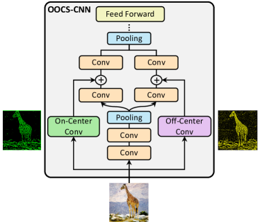
Figure 1: On-off center-surround (OOCS) inductive biases significantly enhance the performance and robustness of a vision network in different lighting conditions.

Finally, a third important motif classifies the center-surround fields into either on-center, when the neurons fire in response to the presence of a light stimulus at the center of their receptive field, and into off-center (OO), when the neurons fire in response to the absence of a light stimulus at the center of their receptive field (Enroth-Cugell & Pinto, 1972). The center-surround motif is also reported to occur in the receptive fields of the primary level visual cortex, causing the so called surround-modulation effect (Hubel & Wiesel, 1965; Knierim & van Essen, 1992; Allman et al., 1985).

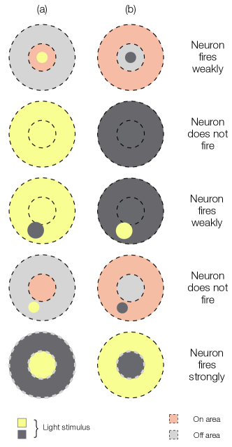
Figure 2: (Kandel et al., 2013)  The response of a) On-center neurons and b) Off-center neurons and their associated receptive fields, respectively, to five different lighting conditions.

As shown in Figures 1-5, the on-off center-surround pathways (OOCS) introduce edge detection inductive biases in a given model. If a light stimulus is turned on at the center of an on-receptive field, but not at its surround, then the on-ganglial neuron fires vigorously. If the light also touches the surround, then the neuron yields a weak response, and ceases to fire in case of a uniform or a surround-only stimulation. This is because of the mutual inhibition of the center and its surround. Complementary, when the light stimulus at the center of an off-receptive field is turned off, but not at its surround, then the off-ganglial neuron fires vigorously. The neuron ceases to fire when the light is turned off at the surround, too (Enroth-Cugell & Pinto, 1972; Kandel et al., 2013). Various studies of retinal circuity have shown that the on-center and off-center ganglial neurons, respectively, are at the origin of two parallel pathways (Callaway, 2005; Zaghloul et al., 2003; Shapley & Perry, 1986). They are physiologically and anatomically distinct, and their receptive fields cover the retinal area completely (Dacey, 2004; Kandel et al., 2013).

Motivated by OOCS in living organisms, we developed a procedure extending any CNN to an OOCS-CNN with same number of parameters, as shown in Figure 1. This first adds the complementary CS convolutional kernels to the input processing. The kernels are fixed and precomputed. Their results are added after one of the original convolutional layers (which intuitively convolve with different kernels, possibly of different sizes). In Figure 1 we add them after the third layer, which worked best on Imagenet. We also split the original layers in two, and concatenate the results thereafter, at the place of addition. Our experiments show that OOCS improves both the performance of CNNs in image recognition tasks, and the robustness of CNNs to challenging illumination conditions. In our experiments with unseen lighting and noisy test sets OOCS-CNNs also outperformed other regularization methods.

Summary of Contributions:

• We introduce OOCS, an inductive edge-detection bias for enhancing the performance and robustness to the variation of lighting conditions of vision networks.

• We prove that on and off residual pathways capture complementary features that improve the generalization error and robustness to distribution shifts.

• We show that OOCS can be applied to any CNN architecture without increasing their number of parameters.

• We conduct an extensive set of experiments showing the superior performance and robustness of OOCS networks compared to standard deep models.

2 Related Work

Receptive field in CNNs. In each convolution layer, a small-sized kernel shifts over the input image, convolving each patch beneath it with the kernel matrix. These kernels were inspired by, and function like the receptive fields (Luo et al., 2016; Li et al., 2019b): they change the activity of the neurons connected to that patch in the next layer (Hubel & Wiesel, 1968; Li et al., 2019a). Fukushima’s Neocognitron (Fukushima, 1980) is arguably the first CNN model to have imported the concept of receptive fields from neural science (Hubel & Wiesel, 1968), and inspired a large body of CNN variants (Fukushima, 2003; LeCun et al., 1989; Lecun et al., 1998; Ciresan et al., 2011; Wang et al., 2019; Ding et al., 2019; Hu et al., 2018).

Bio-inspired Models. A large body of works tried to bringing insights from neuroscience to computer vision systems (Kim et al., 2016; Zoumpourlis et al., 2017; Laskar et al., 2018; Lechner et al., 2020a; Hasani et al., 2021). Fukushima enhanced the Neocognitron model with several priors (Jacobsen et al., 2016), such as contrast-extracting preprocessing layer, inspired by the On-Off ganglial neurons, and inhibitory surround connections, such as the surround-modulation in the visual cortex (Fukushima, 2003). More recent bio-inspired work proposed to replace the feed-forward architecture of CNNs with a recurrent architecture, by adding local-range and long-range feedback connections (Nayebi et al., 2018), or by adding intrinsic horizontal connections (Linsley et al., 2018).

A center-surround architecture is also proposed in (Hasani et al., 2019), in the form of a convolutional layer with a fixed kernel (a difference of Gaussians DoG, as shown in Figures 3(a) and 4(a-b)), to the activation map of the first layer of the network. In a fixed kernel, positive weights are introduced for close neighbor neurons, and negative weights for those that are farther apart. This approach improved the performance of CNNs on various image-classification tasks.

Similar to (Hasani et al., 2019), we also use a DoG kernel with positive weights for the center neurons and negative weights for the surround neurons, as shown in Figures 3(a) and 4(c). However, while (Hasani et al., 2019) uses a DoG kernel similar to (Rodieck, 1965), our work uses the DoG kernel in (Petkov & Visser, 2005; Kruizinga & Petkov, 2000). The disadvantage of (Rodieck, 1965) is that the variances of the Gaussians are unknown. For example, in (Hasani et al., 2019) they are fixed to 1.2 for inhibitory synapses and to 1.4 for excitatory ones. In addition, the DoG in (Rodieck, 1965) may result in very small numbers, that have to be normalized as in (Hasani et al., 2019), for achieving meaningful results. Using the DoG in (Petkov & Visser, 2005; Kruizinga & Petkov, 2000) we do not need to perform a hyperparameter search to find the optimum value for the variances. By just knowing the size of the receptive fields, we can analytically compute the corresponding, large enough, variances. Finally, in contrast to (Hasani et al., 2019), we use both on- and off-pathways (Kim et al., 2016), as shown in Figure 3, and in Figure 4(c) and its complement. These pathways capture complementary features which are lost in the use of either on- or off-pathways alone.

3 Main Results

In this section, we discuss our main findings. We first introduce the structure of the OOCS blocks. We then lay the theoretical grounds for their effectiveness in robustifying deep models to the variation of lighting conditions.

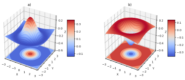
Figure 3: Our difference of Guassians function for a) On and b) Off kernels of size 5 and center to surround ratio of $2/3$.

Center Surround Kernels. Center and surround weights can be computed by a difference of two Gaussian functions (DoG). This difference can be written in Cartesian coordinates (CC), as follows, where the CC origin is taken as the center of the receptive field (Rodieck, 1965):

$$\centering DoG(x,y)=K_{1}\,e^{-\frac{x^{2}+y^{2}}{\sigma_{1}}}-K_{2}\,e^{-\frac{x^{2}+y^{2}}{\sigma_{2}}}\@add@centering$$ (1)

where $K_{1}\,{>}\,K_{2}$ and $\sigma_{2}\,{>}\,\sigma_{1}$ (Blackburn, 1993).

Why the kernel presented by (1) is not optimal? The main disadvantage of this model is that the variances of the Gaussians have to be determined through a hyper-parameter search. The values of the weights calculated are typically too small, and have to be normalized like in (Hasani et al., 2019), to obtain meaningful results, as in Figure 4(b).

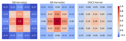
Figure 4: From left to right: Kernel taken from (Hasani et al., 2019) used in their experiments; Actual kernel calculated by their proposed method; Our on-center kernel.

Furthermore, with $K_{i}=1/2\pi\sigma_{i}^{2}$ which is used in (Hasani et al., 2019), the two Gaussian functions take almost equal values for close $\sigma_{1}$ and $\sigma_{2}$. This yields their differences taking very small values everywhere. Normalizing the values to the value of the center, results in loosing the center’s weight in excitation or inhibition.

Improved Center-Surround Kernels. To overcome the shortcomings discussed above, we set out to design an improved kernel, as shown in Figures 3(a-b) and 4(c), based on the DoG model proposed in (Petkov & Visser, 2005; Kruizinga & Petkov, 2000), for defining the difference of Gaussians for the center and surround kernels. This model allows us to analytically compute the variances, from the size of the receptive fields (Petkov & Visser, 2005):

$$DoG_{\sigma,\gamma}(x,y)=\frac{A_{c}}{\gamma^{2}}\,e^{-\frac{x^{2}+y^{2}}{2\gamma^{2}\sigma^{2}}}-A_{s}\,e^{-\frac{x^{2}+y^{2}}{2\sigma^{2}}}$$ (2)

Here, $\gamma$ with $\gamma\,{<}\,1$, defines the ratio between the radius $r$ of the center and that of the surround. We determine the values of the coefficients $A_{c}$ and $A_{s}$ by requiring that the sum of all positive values in Equation (2) are equal to those of the negative values. We normalize this and let their sum be equal to 1 and -1, respectively:

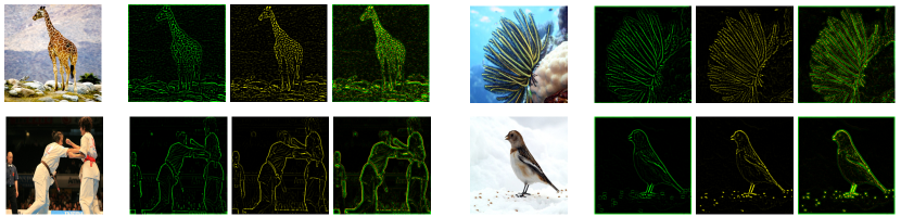
Figure 5: On-center and off-center kernel convolution on samples from Imagenet dataset. The 1st column shows the original image, the 2nd and 3rd columns show on-center and off-center filters respectively. The 4th column shows the filters added together. They extract complementary features within the original image. For example, the bright spot top-left in the Judo image, is properly detected only by the on-center filter, whereas the dark grains on the bottom of the bird image, only by the off-center filter. Hence both filters are necessary.

$$\iint[DoG_{\sigma,\gamma}(x,y)]^{+}dxdy=1,$$ (3)

$$\iint[DoG_{\sigma,\gamma}(x,y)]^{-}dxdy=-1$$ (4)

By $[z]^{+}$ and $[z]^{-}$ we denote the positive and the negative half wave rectification functions, respectively:

$$[z]^{+}=max(0,z),\quad[z]^{-}=min(0,z)$$ (5)

Proposition 1 (DoG Coefficients).

In the infinite continuous case, the coefficients $A_{c}$ and $A_{s}$ are equal.

The proof is given in the supplementary materials. By setting the $DoG_{\sigma,\gamma}(x,y)=0$, and using Proposition 1, we can immediately calculate $\sigma$ as in Equation 6 below, for arbitrary $r$ and $\gamma$. Note that in the finite discrete case, the values of $A_{c}$ and $A_{s}$ are still very similar:

$$\sigma\approx\frac{r}{2\gamma}\sqrt{\frac{1-\gamma^{2}}{-\ln{\gamma}}}$$ (6)

See Supplementary Materials for the complete calculations.

This model not only allows us to find the variance of the kernels analytically, but also it overcomes the normalization issues of (1). The weights calculated by Eq. (2) do not have to be normalized and can be obtained by the kernel size and the ratio of the center to surround. Moreover, forcing the positive and negative weights to sum up to 1 and -1 results in a balance between the excitations and inhibitions. There is evidence for this balance in neuroscience (see Figure 2).

In the DoG model of Equation (1) however, the positive and negative weights do not necessarily sum up to zero, unless in very large kernels. We calculated the weights of the SM kernel in Figure 4(b) using this equation, with the parameters reported in (Hasani et al., 2019). However, this kernel is different from the one in Figure 4(a), which is actually used in their experiments. This kernel is altered in a way that the positive and negative weights sum up to zero.

On and Off kernel matrices. We use Equation (2) to compute the weights in the On-center kernel matrix $DoG_{\rm On}$. For the Off-center kernel $DoG_{\rm Off}$, we use the same equation with inverted signs. For a given input $\chi$, we calculate the On and Off responses by convolving $\chi$ with the computed kernels separately:

$$\chi_{\rm On}[x,y]=(\chi*DoG_{\rm On})[x,y],$$ (7)

$$\chi_{\rm Off}[x,y]=(\chi*DoG_{\rm Off})[x,y]$$ (8)

It is important to note that both the on-convolution and the off-convolution covers the entirety of the input image.

Designing OOCS Pathways. As shown in Figure 1, we add the computed responses to the activation maps of the first layers in the on- and off-pathways, respectively. To implement the on-off residual maps, we split the CNN layers between the on and off parallel pathways, with half of the number of the filters of the original layers, in the layers of each pathway. Thus, the number of the training parameters remains unchanged. At the end of the pathways, we concatenate the activation maps of the last on and off layers, and feed this to the rest of network. The system is structured and trained via Algorithm 1. The on-off pathways are residual connections to facilitate the training process while enhancing the network’s robustness to illuminations.

Algorithm 1 Building and Training OOCS networks

  Inputs: mini batches $\mathcal{B}$, Network $N$ with layers $L=\{l_{1},\dots,l_{n}\}$ parametrized by $\theta$, $l_{i,1/2}=$ half of layer $l_{i}$ DoG center radius $r$, Center-Surround ratio $\gamma$.

  Output: OOCS Network

  for $j$ in Number of Training Steps do

     for $b$ in $\mathcal{B}$ do

        $x_{\emph{on}}=l_{1,1/2}(b)+b*DoG_{on}(b,r,\gamma)$;

        $x_{\emph{off}}=l_{1,1/2}(b)+b*DoG_{off}(b,r,\gamma)$;

        $x_{\emph{new}}$ = Concatenate($l_{2,1/2}(x_{on})$, $l_{1,1/2}(x_{\emph{off}})$) 

        Construct the rest of $N$ on $x_{new}$ as input.

        $L_{total}=\sum_{j=1}^{T}L(y_{j},\hat{y}_{j})$,   $\nabla L(\theta)=\frac{\partial L_{tot}}{\partial\theta}$

        $\theta=\theta-\alpha\nabla L(\theta)$

     end for

  end for

  Return $N_{\theta}$

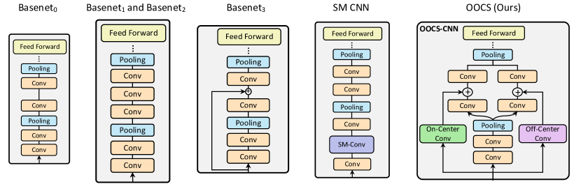
Figure 6: The network architecture for the Basenets, SM CNN and our OOCS-CNN.

OOCS blocks can be used to extend any deep model, without the need to search for optimal hyperparameters for the on and the off kernels. Figure 5 shows the saliency maps of on-convolution, off-convolution, and the combined convolution, for four samples taken from the Imagenet dataset (Deng et al., 2009). The OOCS kernels detect unique edge patterns, by extracting positive and negative contrasts. While they both detect edges, they do this in complementary ways. For a dark feature on a light background, the on-convolution detects the outer edges, and the off-convolution detects the inner ones. For a light feature on a dark background, roles are reversed. More importantly, the strength of the responses is different in the extracted edges, since the on-convolution and the off-convolution have a complementary response to light, as shown in Figure 2 (rows 1,3,5). This means that some of the features extracted by one of the convolutions are not present in the other, or they appear very weak.

Theorem 1 (On-Off Complementarity).

The on- and off-pathways learn unique and complementary features.

The proof of Theorem 1 is given in Supplementary Materials. It uses the definition and the associated properties (eg., Proposition 1) of the on- and off-convolutions. Theorem 1 demonstrates that it is not enough to use either the on- or the off-convolution, alone. Both are required to maximize information flow, in accurate and robust image recognition.

4 Experimental Evaluation

We perform two sets of experiments. In Section 4.1, we evaluate OOCS on standard image classification benchmarks, and compare its performance to competitive baselines. We also perform a couple of ablation analyses on the baseline networks and OOCS to validate our observations.

In Section 4.2, we perform a rigorous robustness analysis, by shifting the test distribution from the training set (Out of IID setting). In particular, we evaluate our models under various challenging lighting condition, as well as on the MNIST data set with black-white inverted images.

Table 1: Top-1 test accuracy and associated variance of the control models and our different OOCS models on Imagenet. n=6

Models Accuracy Basenet₀    (standard deep CNN) 40.8 $\pm$ 0.4 Basenet₁    (extra convolution with ReLU) 39.4 $\pm$ 0.6 Basenet₂    (extra convolution) 41.0 $\pm$ 0.5 Basenet₃    (extra skip connection) 42.1 $\pm$0.5 Basenet₄    (5x5 kernel skip connection) 42.0 $\pm$0.6 Basenet₅    (OOCS without on/off kernels) 41.3 $\pm$0.7 SM-CNN₀  (kernel given in Figure 4a) 38.1 $\pm$ 0.6 SM-CNN₁  (kernel given in Figure 4b) 37.0 $\pm$ 0.4 SM-CNN₂  (kernel given in Figure 4c) 41.9 $\pm$ 0.8 OOCS₀  (on-kernel given in Figure 4c) 44.4 $\pm$ 0.3 OOCS₁  (kernel size 3x3, CS ratio 1/2) 43.4 $\pm$ 0.5 OOCS₂  (OOCS weights $1/n_{c}$ and $1/n_{s}$) 43.6 $\pm$ 0.6 OOCS₃  (OOCS computed after first pool) 44.1 $\pm$ 0.4 OOCS₄  (OOCS with trainable kernels) 44.5 $\pm$ 0.9

We implemented all models in TensorFlow 2.3 (Abadi et al., 2016), and used Adam for optimization (Diederik & Ba, 2015) with a learning rate of $10^{-4}$. We repeated all of the experiments for six times and report the mean value of the obtained results, together with their standard deviation. The latter was computed with a confidence level of 99.9%.

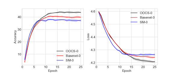
Figure 7: Validation accuracy and loss of the Basenet₀, OOCS₀, and SM-CNN₀ across epochs.

4.1 Image Classification

In this section, we assess the performance (accuracy) of OOCS models in image classification tasks.

Dataset. We used a subset of the Imagenet (Deng et al., 2009). We randomly chose 600 samples from 100 categories. From these samples, we used 500 of each class for the training set, and 50 for each of the validation and test sets. After cropping all the rectangular images to squares around the center, we resized all the images to $192\times 192$ pixels. We did not perform any preprocessing on the images.

Architectural details. We use three main architectures for this experiment as shown in Figure 6: Basenet₀, SM-CNN₀, and OOCS₀. We start from a standard deep CNN architecture for image recognition that we call Basenet₀. It consists of seven convolutional layers, five max-pooling layers, and two fully connected layers. All convolutional layers have $3\times 3$ kernels and strides of 1. We initialized all kernels with the He initialization (He et al., 2015). The max-pooling layers have $2\times 2$ kernels and strides of 2. Dropouts (Srivastava et al., 2014) follow the fully connected layers, and the last layer predicts the category with a softmax function. All of the hidden-weight layers have ReLU activation functions. We have also three other variations Basenet₁, Basenet₂ and Basent₃ discussed in the ”what happens” paragraph below.

We use the Surround-Modulation model of (Hasani et al., 2019) for SM-CNN₀, with the kernel given in Figure 3(b). Although SM and OO retinal receptive fields are two distinct biological phenomena, there are similarities between them and the way they are modeled. To ensure fairness, for the SM-CNN, we added the SM kernel to the activation maps of the first convolution layer in our baseline CNN, precisely aligned with what the authors suggested, and used the kernel weights they have reported. The variants SM-CNN_1-2 are described below in ”what happens”..

For the OOCS-CNN network OOCS₀, we split the convolutional layers between the first and second pooling layers, into two parallel pathways with half of the filters of the original layers in each. The on-response is calculated by convolution with the on-kernel given in Figure 3(c) and the off-response with its complementary kernel. The weights of these kernels are specified as non-trainable parameters.

Performance. We compared the test accuracy of OOCS₀ with the performance of the Basenet₀ and of SM-CNN₀. Figure 7 shows the validation accuracy and loss for the three main network variants. As one can see, OOCS₀ outperforms the others by a large margin. Moreover, one can observe that SM-CN₀ has a better sample efficiency as it is stated in (Hasani et al., 2019), but has a poor performance on the validation set in comparison to the Basenet₀.

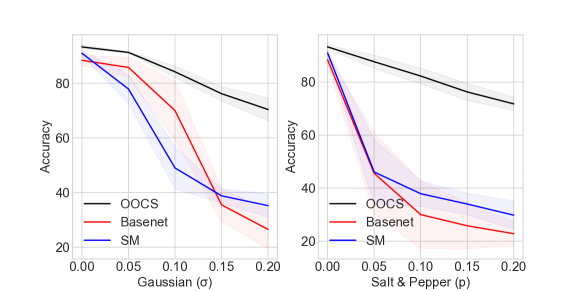
Figure 8: Noise-robustness. Test accuracy of the OOCS-CNN, the SM-CNN and the Basenet as a function of increasing input noise variance, with illumination Light0, and with n=6

What happens if we alter the architectures? To more thoroughly evaluate OOCS performance, we designed eleven additional network variants: Basenet_1-5, SM-CNN_1-2, and OOCS_1-4. Basenet_1-2 were designed by adding an extra layer to Basenet₀, to see whether the performance of OOCS₀ can be obtained by increasing the number of training parameters of Basenet₀. This extra layer was added between the first and second pooling layers, with 64 filters. This new layer has a ReLU activation function in Basenet₁, and no activation function in Basenet₂. Basenet_3-4, have a skip-connection from the input to the output of the third convolution layer of Basenet₀, thus constructing a residual block (He et al., 2016). This investigates if the performance of OOCS₀ is in fact related to the skip connection between the input and on-off pathways. The skip connection in Basenet₄ is a convolution layer with $5\times{}5$ kernel. Finally, Basenet₅ has the exact same architecture of OOCS₀, with the parallel pathways but with trainable filters alongside the skip connections. The kernels are initialised with the He initialization (He et al., 2015).

SM-CNN₁ uses the kernel given in Figure 4(b), which is calculated from the DoG proposed by (Hasani et al., 2019), in Equation (1). We also designed an extra variant, called SM-CNN₂, which uses the OOCS kernel for the on-center-surround DoG, and which is given in Figure 4(c).

OOCS₁ uses a smaller kernel to perform the convolutions: $3\times{}3$ as the size for the receptive field, and $\gamma\,{=}\,1/2$ as the center-surround ratio. OOCS₂ uses $1/n_{c}$ and $1/n_{s}$ as the weights for the elements in the center and surround in the kernel matrix, respectively, where $n_{c}$ is the number of central elements and $n_{s}$ is the number of elements in the surround. The aim was to indicate the effectiveness of the proposed DoG model. OOCS₃ computes the on- and off-responses from the inputs to the first layers of the pathways and adds them to the activation maps of the first layers in the pathways. Finally, OOCS₄ has the same architecture of OOCS₀, but with trainable filters on the On and Off skip connections, initialised with the On and Off kernels. Table 1 shows the top-1 test accuracy for the main and control networks. This model was added to see whether the On and Off kernels structure will be reserved throughout the training or we will eventually converge to other settings. All $64$ filters kept the OOCS structure, with differences in on and off weights intensities. OOCS₀ and it’s variants OOCS_1-4 outperform all other models.

The results suggest that OOCS₀ performance can neither be achieved by increasing the capacity of Basenet₀ nor by adding skip-connections to Basenet₀. Moreover, the results for Basenet${}_{4}-5$ show that the On-Off Center-Surround structure can not be learned by network without initialising or fixing the kernels with the calculated On and Off kernels. The On Center-Surround kernel of OOCS₀ also increases the performance of SM-CNN₀ considerably, and outperforms Basenet₀. Finally, SM-CNN₁ has a lower accuracy than Basenet₀.

The accuracy of OOCS₁ shows that with a smaller kernel, one still outperforms the Basenets and the SM-CNNs, but it decreases the accuracy compared to Basenet₀. OOCS₂ achieved a higher accuracy than these networks, too. This shows that forcing the positive and negative parts of the kernel to sum up to 1 and -1 respectively plays an important role in the OOCS-CNN’s superior performance. Finally, OOCS₃ also outperforms the Basenets and SM-CNNs.

OOCS ResNet. Here we modify the architecture of a residual network(He et al., 2016) to include OOCS and evaluate the performance of it with and without the OOCS filters.

Dataset. In this experiment, we use the same subset of Imagenet. We augmented the training images with randomly rotating them in the range of $15$, randomly shifting horizontally and vertically in the range of 10 percent of total width and height, and randomly flipping the images horizontally.

Table 2: Top-1 test accuracy and associated variance of the Resnet34 and Resnet34-OOCS models on Imagenet. n=6

Models	Acc
ResNet34	61.73 $\pm$ 0.6
ResNet34-OOCS	63.39 $\pm$ 0.7

Architectural details and Performance. We used the ResNet34(He et al., 2016) as the base network. In order to add OOCS to it, we splitted the first two layers of the first residual block into the On and Off pathways with half of the filters of the original layers in each. The On and Off responses were calculated from the inputs to the first residual block.

As Table 2 shows the results for both networks, OOCS enhances the performance of larger networks like ResNets and does not lose its effectiveness with data augmentation.

Table 3: Test Accuracy on all 6 lighting conditions for networks trained on Light0. n=6.

	Familiar Test Set	Unfamiliar Test Set
Models	Light0	Light1	Light2	Light3	Light4	Light5
Basenet	88.4 $\pm$ 1.9	82.2 $\pm$ 2.4	46.4 $\pm$ 4.1	86.2 $\pm$ 1.5	58.8 $\pm$ 2.7	79.5 $\pm$ 4.9
Basenet-L2	89.6 $\pm$ 1.9	87.0 $\pm$ 2.8	48.5 $\pm$ 3.8	86.9 $\pm$ 1.5	60.8 $\pm$ 3.5	80.3 $\pm$ 4.5
Basenet-Dropout	89.2 $\pm$ 2.0	86.3 $\pm$ 5.7	48.5 $\pm$ 4.1	86.3 $\pm$ 1.2	59.9 $\pm$ 3.8	81.3 $\pm$ 5.4
Basenet-BN	89.2 $\pm$ 1.4	84.0 $\pm$ 3.7	37.4 $\pm$ 7.7	87.3 $\pm$ 2.0	56.2 $\pm$ 3.7	78.9 $\pm$ 4.4
SM-CNN	91.0 $\pm$ 0.9	90.6 $\pm$ 0.6	62.5 $\pm$ 1.5	87.3 $\pm$ 1.6	61.8 $\pm$ 2.3	81.6 $\pm$ 1.7
OOCS-CNN (Ours)	93.3 $\pm$ 0.7	90.9 $\pm$ 0.7	56.7 $\pm$ 1.6	91.2 $\pm$ 1.0	61.9 $\pm$ 1.5	88.2 $\pm$ 1.0

4.2 Robustness Evaluation

Here we evaluate OOCS robustness. To this end we extensively study how deep CNN models perform under the variation of lighting conditions and to distribution shifts.

Dataset. We used the Norb dataset (LeCun et al., 2004) to assess the robustness of our proposed OOCS-CNN architecture. This dataset contains images of 3D objects belonging to five generic categories. The images are of size $96\,{\times}\,96$ pixels, and photographed under six different lighting conditions. In a first experiment, we trained our networks on the images from one lighting condition, Light0, and then tested them on all six lighting conditions. In a second experiment we added different kinds of noise to the testing images, in order to evaluate the robustness in the presence of noise.

Architectural details. Given the image size, we designed CNN Basenets with 6 convolutional layers, 4 max-pooling layers, and 2 fully connected layers. All convolutional layers have $3\times 3$ kernels, and strides of 1. The max-pooling layers have $2\times 2$ kernels and strides of 2. The number of filters in the first convolution layer is 32 and gets doubled after each pooling layer. For the OOCS-CNN, we split the layers between the first and second max-pooling to On and Off pathways and compute the On and Off convolutions from the input to the first layers of pathways.

Robustness Evaluation. To assess the robustness of OOCS-CNNs under changes in illumination, we tested the networks on images with a lighting condition that was different from the one in the training set. We compare the performance of our model with Basenet-L2, Basenet-Dropout and Basenet-BN, in addition to the Basenet and SM-CNN.

Table 4: Test Accuracy and variance for images from Light0 with Gaussian noise for networks trained on Light0. n=6.

Gaussian Noise ($\sigma$) Models 0.05 0.1 0.15 0.2 Basenet $85.8_{\pm 3.6}$ $70.0_{\pm 10.8}$ $35.5_{\pm 5.9}$ $26.5_{\pm 7.1}$ Basenet-L2 $84.8_{\pm 2.0}$ $73.3_{\pm 3.9}$ $46.0_{\pm 10.4}$ $33.0_{\pm 8.1}$ Basenet-D $87.5_{\pm 2.9}$ $80.8_{\pm 2.4}$ $66.5_{\pm 11.7}$ $42.2_{\pm 17.7}$ Basenet-BN $84.4_{\pm 2.8}$ $69.8_{\pm 10.3}$ $48.8_{\pm 13.3}$ $38.4_{\pm 8.3}$ SM-CNN $77.9_{\pm 5.2}$ $49.0_{\pm 7.7}$ $38.8_{\pm 2.6}$ $35.2_{\pm 4.2}$ OOCS-CNN $\mathbf{91.3_{\pm 0.3}}$ $\mathbf{84.2_{\pm 2.1}}$ $\mathbf{76.2_{\pm 2.6}}$ $\mathbf{70.4_{\pm 4.0}}$

Table 5: Test Accuracy and variance for images from Light0 with Salt & Pepper noise for networks trained on Light0. n=10.

Salt and Pepper Noise ($p$) Models 0.05 0.1 0.15 0.2 Basenet $45.6_{\pm 15.3}$ $30.0_{\pm 12.7}$ $25.8_{\pm 8.7}$ $22.8_{\pm 4.5}$ Basenet-L2 $49.7_{\pm 9.4}$ $31.6_{\pm 7.5}$ $26.0_{\pm 5.4}$ $23.7_{\pm 3.5}$ Basenet-D $71.5_{\pm 7.5}$ $48.5_{\pm 13.3}$ $29.1_{\pm 12.1}$ $22.1_{\pm 3.5}$ Basenet-BN $54.2_{\pm 14.7}$ $40.6_{\pm 13.0}$ $34.2_{\pm 10.8}$ $29.7_{\pm 8.3}$ SM-CNN $46.1_{\pm 12.3}$ $37.9_{\pm 4.8}$ $34.0_{\pm 4.1}$ $29.8_{\pm 5.3}$ OOCS-CNN $\mathbf{87.7_{\pm 2.5}}$ $\mathbf{82.3_{\pm 3.0}}$ $\mathbf{76.3_{\pm 3.2}}$ $\mathbf{71.8_{\pm 2.5}}$

Table 3 shows the test-accuracy and associated variance for all baselines trained on Light0. Except for Light2, where SM-CNN proved to be superior to the other networks, the OOCS-CNN outperformed the other CNN variants with a considerable margin.

We then added Gaussian and Salt $\&$ Pepper noise to the test set, to evaluate the performance of the networks under perturbations. Table 4 and Table 5 show the test accuracy and variance for networks, trained on Light0 and tested on the same lighting condition, but in the presence of noise.

The results show that the OOCS-CNN is more robust than other regularization methods. Not only has it higher accuracy, the results of the OOCS-CNN have considerably lower variance in comparison to the other networks on modified test sets. Figure 8 shows the significant level of robustness to noise achieved by OOCS compared to other methods.

Robustness to distribution shifts. As discussed before, on- and off-convolutions extract different features for objects on light and dark backgrounds. Both are needed to capture higher details. To assess our claim more thoroughly, we designed the following experiment.

Dataset. We used the MNIST dataset (LeCun & Cortes, 2010) to train our networks. The original dataset contains black handwritten digits on white background. We trained our networks on the original images, but for the test set we altered all the pixel values by subtracting them from $255.$ Figure 9 shows the original/altered image for one sample.

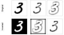
Figure 9: The on- and off-convolutions are shown in the second and the third columns, respectively, for a sample of the MNIST dataset. In the first row we show the original image, and in the second row the inverted image, with all pixels subtracted from 255.

Table 6: Test Accuracy of the networks on the original black-on-white and on the inverted white-on-black test sets. n=6.

	Basenet	SM-CNN	OOCS-CNN
Original	$99.1_{\pm 0.2}$	$99.2_{\pm 0.1}$	$99.1_{\pm 0.2}$
Inverted	$29.0_{\pm 10.1}$	$35.7_{\pm 4.9}$	$\mathbf{93.9_{\pm 1.2}}$

Robustness evaluation. Table 6 shows the test accuracy of the networks on the original and altered MNIST test images. On the test set with inverted colors, the accuracy of the Basenet and SM-CNN drops sharply. The OOCS-CNN on the other hand, achieves a much higher accuracy on this challenging test set. Figure 9 shows that on the samples with black foreground, the on-center convolution extracts features similar to the ones extracted by the off-center convolution on the samples with black background and vice versa. Being equipped with both in OOCS-CNN is the reason it still performs better on the altered test set.

5 Discussion, Scope and Conclusions

Inspired by the retinal ganglial cells in vertebrates, we first proposed an on-off center-surround (OOCS) enhancement to the receptive fields of vision networks. We then showed that the OOOCS pathways impose an inductive bias on the vision networks, which enhances their robustness to the variation of lighting conditions. We took advantage of the studies in the field of Neuroscience and used an improved CS kernel as a ubiquitous block for obtaining more accurate and more robust vision based networks. The OOCS addition to a CNN is easy to implement, does not increase the number of trainable parameters, and it increases its performance.

Performance Out of IID Setting. OOCS performs extremely well under test-set distribution-shifts. This is a direct result of the complementary on- and off-pathways.

Inductive Biases vs. Regularization. Our experiments (Table 2) show that standard regularization methods such as L2, Dropout and batch-normalization are less effective in improving generalization under distribution shifts, compared to the OOCS. Figure 10 gives the absolute distance of the familiar test error (of the same lighting condition as the training set), to the test error of different lighting conditions. We observe that OOCS has a lower distance for distribution shifts compared to regularization methods.

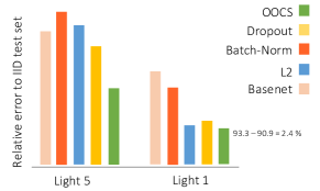
Figure 10: Relative test error for different lighting conditions compared to the IID test error (shorter bar is better). The values are taken from Table 3. Each bar represents the deviation of the test error from the test error for Light0.

Robustness to Digital Distribution Shifts. What happens if we add OOCS filters to a ResNet architecture? would this improve their robustness properties to distribution shifts such as Gaussian perturbations, brightness, and contrast. We studied this systematically in a set of experiments where we added OOCS filters to a ResNet-34, and compared its performance under variation of these perturbations (See Figures S3 and S4 in the supplementary materials). We observed consistent improvements achieved when OOCS filters are deployed.

Usability and Impact of OOCS Blocks. OOCS pathways can be added to any vision-based model regardless of their exact architecture. They can be interpreted as targeted residual blocks explicitly designed to perform specialized edge detection. In decision critical applications (Lechner et al., 2019, 2020a), object recognition under different lighting conditions is a game changer. For instance vision-based self-driving cars are sensitive to lighting conditions (Lechner et al., 2021, 2020b). OOCS can robustify driving under direct sun or going from shaded to well lit regions.

Bio-inspirations and Future Work. In this work, our main focus was to bring insights from a simplified model of the retinal cells to designing more robust image classification modules. There are additional top-down connections between layers in the retina, and the sizes of the receptive fields change depending on their location. It is therefore worth exploring the implementation of a complete model of the retina and to further improving the performance of this model, similar to many works that aim to transform biological mechanisms (Lechner et al., 2017; Sarma et al., 2018; Gleeson et al., 2018; Dabney et al., 2020) into better machine learning models (Hasani et al., 2020). The OOCS helps a network to extract the inner and outer edges, hence more work can be done to investigate using it as a preprocessing or data augmentation tool, especially for medical image segmentation tasks.

Appendix S1 Theoretical Proofs and Calculations

In this section, we bring the mathematical calculations and theoretical proofs.

S1.1 Proof of Proposition 1

The DoG model used in the main document is defined as in Equation (2), where $\gamma$ with $\gamma\,{<}\,1$, defines the ratio between the radius $r$ of the center and that of the surround. This model allows us to analytically compute the variances, from the size of the receptive fields:

$$DoG_{\sigma,\gamma}(x,y)=\frac{A_{c}}{\gamma^{2}}\,e^{-\frac{x^{2}+y^{2}}{2\gamma^{2}\sigma^{2}}}-A_{s}\,e^{-\frac{x^{2}+y^{2}}{2\sigma^{2}}}$$ (S1)

The coefficients $A_{c}$ and $A_{s}$ are determined, by requiring that the sum of all positive values in Equation (S1) are equal to those of the negative values. Here, we make them to sum up to 1 and to -1, respectively:

$$\iint[DoG_{\sigma,\gamma}(x,y)]^{+}dxdy=1,$$ (S2)

$$\iint[DoG_{\sigma,\gamma}(x,y)]^{-}dxdy=-1$$ (S3)

By $[z]^{+}$ and $[z]^{-}$ we denote the positive and the negative half wave rectification functions, respectively:

$$[z]^{+}=max(0,z),\quad[z]^{-}=min(0,z)$$ (S4)

Proposition 2 (DoG Coefficients).

In the infinite continuous case, the coefficients $A_{c}$ and $A_{s}$ are equal.

Proof.

We have the following equalities:

$$\iint_{\mathbb{R}^{2}}[\frac{A_{c}}{\gamma^{2}}\,e^{-\frac{x^{2}+y^{2}}{2\gamma^{2}\sigma^{2}}}-A_{s}\,e^{-\frac{x^{2}+y^{2}}{2\sigma^{2}}}]^{+}dxdy=1,$$ (S5)

$$\iint_{\mathbb{R}^{2}}[\frac{A_{c}}{\gamma^{2}}\,e^{-\frac{x^{2}+y^{2}}{2\gamma^{2}\sigma^{2}}}-A_{s}\,e^{-\frac{x^{2}+y^{2}}{2\sigma^{2}}}]^{-}dxdy=-1$$ (S6)

By transforming the integrals to the polar coordinates we have the equations below, where $r_{s}$ is the radius of the surround, and $r_{s}\to\infty$.

$$\int_{0}^{2\pi}\int_{0}^{r_{s}}[\frac{A_{c}}{\gamma^{2}}\,r\,e^{-\frac{r^{2}}{2\gamma^{2}\sigma^{2}}}-A_{s}\,r\,e^{-\frac{r^{2}}{2\sigma^{2}}}]^{+}drd\theta=1,$$ (S7)

$$\int_{0}^{2\pi}\int_{0}^{r_{s}}[\frac{A_{c}}{\gamma^{2}}\,r\,e^{-\frac{r^{2}}{2\gamma^{2}\sigma^{2}}}-A_{s}\,r\,e^{-\frac{r^{2}}{2\sigma^{2}}}]^{-}drd\theta=-1$$ (S8)

The positive values are in the center with radius of $r_{c}$ and the negative values are in a ring between the center and surround. So we can remove the half wave rectifiers as follows:

$$2\pi\int_{0}^{r_{c}}\frac{A_{c}}{\gamma^{2}}\,r\,e^{-\frac{r^{2}}{2\gamma^{2}\sigma^{2}}}-A_{s}\,r\,e^{-\frac{r^{2}}{2\sigma^{2}}}\,dr=1,$$ (S9)

$$2\pi\int_{r_{c}}^{r_{s}}\frac{A_{c}}{\gamma^{2}}\,r\,e^{-\frac{r^{2}}{2\gamma^{2}\sigma^{2}}}-A_{s}\,r\,e^{-\frac{r^{2}}{2\sigma^{2}}}\,dr=-1$$ (S10)

After calculating the integrals:

$$2\pi(A_{c}\,\sigma^{2}\,e^{-\frac{r^{2}}{2\gamma^{2}\sigma^{2}}}-A_{s}\,\sigma^{2}\,e^{-\frac{r^{2}}{2\sigma^{2}}})\Big{|}_{0}^{r_{c}}=1,$$

$$2\pi(A_{c}\,\sigma^{2}\,e^{-\frac{r^{2}}{2\gamma^{2}\sigma^{2}}}-A_{s}\,\sigma^{2}\,e^{-\frac{r^{2}}{2\sigma^{2}}})\Big{|}_{r_{c}}^{r_{s}}=-1$$

$$2\pi\sigma^{2}(A_{c}\,e^{-\frac{r_{c}^{2}}{2\gamma^{2}\sigma^{2}}}-A_{s}\,e^{-\frac{r_{c}^{2}}{2\sigma^{2}}})-2\pi\sigma^{2}(A_{c}\,e^{0}-A_{s}\,e^{0})=1,$$

$$2\pi\sigma^{2}(A_{c}\,e^{-\frac{r_{s}^{2}}{2\gamma^{2}\sigma^{2}}}-A_{s}\,e^{-\frac{r_{s}^{2}}{2\sigma^{2}}})-2\pi\sigma^{2}(A_{c}\,e^{-\frac{r_{c}^{2}}{2\gamma^{2}\sigma^{2}}}-A_{s}\,e^{-\frac{r_{c}^{2}}{2\sigma^{2}}})=-1$$ (S11)

Adding the two equations together, we have:

$$\lim_{r_{s}\to\infty}2\pi\sigma^{2}(A_{c}\,e^{-\frac{r_{s}^{2}}{2\gamma^{2}\sigma^{2}}}-A_{s}\,e^{-\frac{r_{s}^{2}}{2\sigma^{2}}})-2\pi\sigma^{2}(A_{c}-A_{s})=0$$

$$=2\pi\sigma^{2}(A_{c}\,e^{-\infty}-A_{s}\,e^{-\infty})-2\pi\sigma^{2}(A_{c}-A_{s})=0$$

$$2\pi\sigma^{2}(A_{c}-A_{s})=0\Rightarrow A_{c}=A_{s}$$ (S12)

∎

S1.2 Computation of the Variance

The $DoG_{\sigma,\gamma}(x,y)$ is equal to zero on the border of the center and surround. The radius equals to $r_{c}$ on this border, meaning that $x^{2}+y^{2}=r_{c}^{2}$ when $DoG_{\sigma,\gamma}(x,y)=0$. so by setting the $DoG_{\sigma,\gamma}(x,y)=0$ we have:

$$\frac{A_{c}}{\gamma^{2}}\,e^{-\frac{r_{c}^{2}}{2\gamma^{2}\sigma^{2}}}-A_{s}\,e^{-\frac{r_{c}^{2}}{2\sigma^{2}}}=0$$

$$\ln(A_{c})-2\ln(\gamma)-\frac{r_{c}^{2}}{2\gamma^{2}\sigma^{2}}-\ln(A_{s})+\frac{r_{c}^{2}}{2\sigma^{2}}=0$$

$$\ln(A_{c})-\ln(A_{s})-2\ln(\gamma)=\frac{r_{c}^{2}}{2\gamma^{2}\sigma^{2}}-\frac{r_{c}^{2}}{2\sigma^{2}}$$

$$\ln(\frac{A_{c}}{A_{s}})-2\ln(\gamma)=\frac{r_{c}^{2}(1-\gamma^{2})}{2\gamma^{2}\sigma^{2}}$$

$$\sigma^{2}=\frac{r_{c}^{2}(1-\gamma^{2})}{2\gamma^{2}(\ln(\frac{A_{c}}{A_{s}})-2\ln(\gamma))}$$

$$\sigma=\frac{r_{c}}{\gamma}\sqrt{\frac{1-\gamma^{2}}{2\ln(\frac{A_{c}}{A_{s}})-4\ln(\gamma)}}$$ (S13)

Based on Proposition 1, the values of $A_{c}$ and $A_{s}$ are equal in the infinite continuous case. Since in the finite discrete case those values are very close, we can approximate the value of $\sigma$:

$$\sigma\approx\frac{r_{c}}{2\gamma}\sqrt{\frac{1-\gamma^{2}}{-\ln{\gamma}}}$$ (S14)

S1.3 Proof of Theorem 1

We use Equation (S1) to compute the weights in the On-center kernel matrix $DoG_{\rm On}$. For the Off-center kernel $DoG_{\rm Off}$, we use the same equation with the signs inverted. For a given input $\chi$, we calculate the On and Off responses by convolving $\chi$ with the computed fixed kernels separately:

$$\chi_{\rm On}[x,y]=(\chi*DoG_{\rm On})[x,y],$$ (S15)

$$\chi_{\rm Off}[x,y]=(\chi*DoG_{\rm Off})[x,y]$$ (S16)

Note that the On and Off convolutions cover the input image completely. These two convolutions result in the following equations, when the kernel is in the shape of a square:

$$\chi_{\rm On}[x,y]=\int_{-r_{s}}^{r_{s}}\int_{-r_{s}}^{r_{s}}\chi(x+\rho,y+\tau)\,(\frac{A_{c}}{\gamma^{2}}\,e^{-\frac{\rho^{2}+\tau^{2}}{2\gamma^{2}\sigma^{2}}}-A_{s}\,e^{-\frac{\rho^{2}+\tau^{2}}{2\sigma^{2}}})\,d\rho\,d\tau$$ (S17)

$$\chi_{\rm Off}[x,y]=\int_{-r_{s}}^{r_{s}}\int_{-r_{s}}^{r_{s}}\chi(x+\rho,y+\tau)\,(A_{s}\,e^{-\frac{\rho^{2}+\tau^{2}}{2\sigma^{2}}}-\frac{A_{c}}{\gamma^{2}}\,e^{-\frac{\rho^{2}+\tau^{2}}{2\gamma^{2}\sigma^{2}}})\,d\rho\,d\tau$$ (S18)

Proof of Theorem 1 The on- and off-pathways learn unique and complementary features.

Proof.

We prove this theorem by contradiction. Assume that the features extracted by the On convolution are identical to the features extracted by the Off convolution. Now suppose the input image has a small spot of light (smaller than the center of our kernels) on a dark background. We first convolve this image with an On kernel. If the spot of light lies in the center of the kernel, the convolution will result in a response close to $1$, according to the Equations (S5), (S6), and  (S17). If the spot of light lies in the surround, the convolution will result in a negative response. As a result we obtain an activation map with values close to $1$ where the light spot is located, negative values in the outer edges of the light spot, and zero values everywhere else.

When we convolve the same image with an Off kernel we obtain the following. If the spot of light lies in the center of the kernel, then we obtain a negative response. If it lies in the surround, then it will result in a positive response close to zero, according to the Equations (S5), (S6), and (S18). Hence, the Off convolution results in an activation map with small values in the outer edges of the light spot, negative values where the light spot is located, and zero values everywhere else. Comparing the two activation maps, one can see that: 1) The positive values are in different locations, and 2) These values are close to $1$ for the On activation map, and close to zero for the Off activation map. This contradicts our initial assumption. Note that a similar but complementary argument can be made for an image with a small dark spot on a light background. ∎

Appendix S2 Experimental Setup

Here, we describe the experimental setup for the tasks discussed in Tables 1, 2, 3, 4 and 5.

S2.1 Dataset description

Image classification. We used a random subset of the Imagenet dataset (Deng et al., 2009) with 60000 images from 100 categories. We used 5000 of the images for each of the validation and test sets. All samples were cropped around the center if they were not originally in square shapes, and then resized to $192\times 192$ pixels.

Robustness to illumination change. We used small Norb dataset (LeCun et al., 2004) which contains images of toys from 5 generic categories: human figures, four-legged animals, airplanes, cars and trucks. The images of each category were taken from 10 toy instances in 6 different lighting conditions, 9 elevations, and 18 azimuths. The training set consists of the images from 5 of the instances of each category, and the rest 5 instances are in the test set. Figure S1 shows one sample from each category in each of the lighting conditions. We separated the dataset based on the lighting conditions, and used the images from the first light, Light0, as the training set and tested our networks on testsets from all 6 different lighting conditions. Each of the training and test sets contained 4050 images of size $96\times 96$ pixels.

Robustness to distribution shifts. We used MNIST dataset (LeCun & Cortes, 2010) containing grayscaled images of handwritten digits. There are 60000 and 10000 samples in the training and test sets respectively. For testing, we inverted all the pixel values by subtracting them form 255.

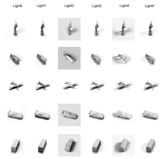
Figure S1: Example samples of the Norb dataset (LeCun et al., 2004) from each of the five categories and each of the lighting conditions.

S2.2 Network architectures and Hyper parameters

For each of the experiments, we used a CNN as the base network, with different numbers of layers depending the dataset image sizes. Figure S2 shows the architectures of the base networks. We construct the other models from the base networks as discussed in the main paper. For the On and Off Center convolutions in OOCS-CNNs, we used kernels of size $5\times 5$ for Imagenet and Norb datasets. We used smaller kernels of size $3\times 3$ for the MNIST dataset, since the images are of smaller size. We calculated the On and Off resposes from the inputs and directly fed their summation to the network.

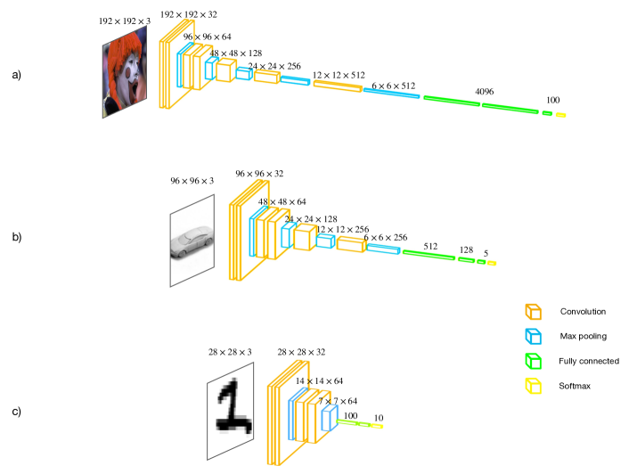
Figure S2: Base network architectures for a) Imagenet subset classification, b) robustness evaluation on Norb, and c) robustness evaluation on MNIST

We had batch sizes of 64 in all experiments. We used Adam optimiser (Diederik & Ba, 2015) for experiments on Imagenet and Norb, with a learning rate of $10^{-4}$. In the experiment on Imagenet, we decreased the learning rate to half after 10 epochs which was mainly in favour of the baselines. In the Imagenet experiments with ResNet-34 we use SGD optimiser and start with a learning rate of 0.1, which we decay by a factor of 0.1 every 20 epochs and we trained the networks for 60 epochs. For scaling the gradient descent steps, we use a Nesterov-momentum of 0.9.

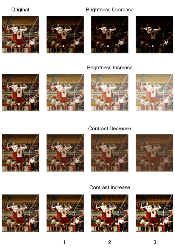
Figure S3: Sample Brightness and contrast variations we tested OOCS and Residual networks against.

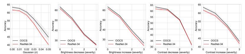
Figure S4: OOCS filters added to ResNet-34 consistently enhances the robustness of a network to perturbations such as Gaussian noise, Brightness and Contrast variations.

Appendix S3 Experiments on Digital Distribution Shifts

In this section we describe the experiments to evaluate the robustness of a ResNet-34 on the Imagnet subset compared to the same network equipped with OOCS.

We altered the test set images with 5 different digital perturbations: adding Gaussian noise, decreasing and increasing the brightness (Gamma correction), and decreasing and increasing the contrast. Figure S3 shows one sample of Imagenet dataset in different brightness and contrast changes with different severities.

The results of this experiment are summarized in tables S1-5 and figure S4. As the results show, OOCS can enhance the robustness of a ResNet under digital distribution shifts.

Table S1: Test Accuracy and variance for test images with Gaussian noise. n=6.

	Gaussian Noise ($\sigma$)
Models	0.01	0.02	0.03	0.04	0.05
ResNet-34	$61.2_{\pm 0.7}$	$58.5_{\pm 0.8}$	$53.14_{\pm 0.8}$	$46.4_{\pm 0.5}$	$40.23_{\pm 0.8}$
OOCS-ResNet-34	$\mathbf{62.7_{\pm 0.7}}$	$\mathbf{60.4_{\pm 0.9}}$	$\mathbf{56.0_{\pm 1.3}}$	$\mathbf{50.5_{\pm 2.1}}$	$\mathbf{44.8_{\pm 2.5}}$

Table S2: Test Accuracy and variance for test images with decreasing brightness. n=6.

	Gamma Correction ($\gamma$)
Models	2	3	4
ResNet-34	$50.9_{\pm 0.5}$	$35.6_{\pm 0.7}$	$25.5_{\pm 0.8}$
OOCS-ResNet-34	$\mathbf{52.3_{\pm 0.9}}$	$\mathbf{36.4_{\pm 0.7}}$	$\mathbf{26.0_{\pm 1.0}}$

Table S3: Test Accuracy and variance for test images with increasing brightness. n=6.

	Gamma Correction ($\gamma$)
Models	1/2	1/3	1/4
ResNet-34	$52.7_{\pm 0.7}$	$36.9_{\pm 1.0}$	$23.7_{\pm 0.2}$
OOCS-ResNet-34	$\mathbf{54.2_{\pm 0.7}}$	$\mathbf{39.3_{\pm 0.7}}$	$\mathbf{26.2_{\pm 1.5}}$

Table S4: Test Accuracy and variance for test images with decreasing contrast. n=6.

	Contrast Factor
Models	0.8	0.6	0.4
ResNet-34	$60.8_{\pm 0.5}$	$52.4_{\pm 0.2}$	$\mathbf{31.8_{\pm 0.9}}$
OOCS-ResNet-34	$\mathbf{61.5_{\pm 0.2}}$	$\mathbf{52.9_{\pm 0.5}}$	$31.7_{\pm 0.8}$

Table S5: Test Accuracy and variance for test images with increasing contrast. n=6.

	Contrast Factor
Models	1.2	1.4	1.6
ResNet-34	$58.4_{\pm 0.6}$	$51.6_{\pm 0.8}$	$41.9_{\pm 1.3}$
OOCS-ResNet-34	$\mathbf{59.9_{\pm 0.9}}$	$\mathbf{52.62_{\pm 0.8}}$	$\mathbf{43.25_{\pm 0.9}}$

Appendix S4 Code and Data Availability

All code and data are included in https://github.com/ranaa-b/OOCS.

References

- Abadi et al. (2016) Abadi, M., Barham, P., Chen, J., Chen, Z., Davis, A., Dean, J., Devin, M., Ghemawat, S., Irving, G., Isard, M., Kudlur, M., Levenberg, J., Monga, R., Moore, S., Murray, D., Steiner, B., Tucker, P., Vasudevan, V., Warden, P., Wicke, M., Yu, Y., and Zheng, X. Tensorflow: A System for Large-Scale Machine Learning. In 12th USENIX Symposium on Operating Systems Design and Implementation (OSDI 16), pp. 265–283, Savannah, GA, November 2016. USENIX.
- Allman et al. (1985) Allman, J., Miezin, F., and McGuinness, E. Stimulus specific responses from beyond the classical receptive field: Neurophysiological mechanisms for local-global comparisons in visual neurons. Annual Review of Neuroscience, 8(1):407–430, 1985.
- Azzopardi et al. (2014) Azzopardi, G., Rodríguez-Sánchez, A., Piater, J., and Petkov, N. A push-pull corf model of a simple cell with antiphase inhibition improves snr and contour detection. PLOS ONE, 9(7):1–13, 07 2014. doi: 10.1371/journal.pone.0098424.
- Blackburn (1993) Blackburn, M. A Simple Computational Model of Center-Surround Receptive Fields in the Retina. Technical Report 2454, Ocean Surveillance Center, Feb 1993.
- Callaway (2005) Callaway, E. Structure and Function of Parallel Pathways in the Primate Early Visual System. The Journal of Physiology, 566(1):13–19, 2005.
- Ciresan et al. (2011) Ciresan, D., Meier, U., Masci, J., Gambardella, L., and Schmidhuber, J. Flexible, High Performance Convolutional Neural Networks for Image Classification. International Joint Conference on Artificial Intelligence IJCAI-2011, pp. 1237–1242, 07 2011.
- Dabney et al. (2020) Dabney, W., Kurth-Nelson, Z., Uchida, N., Starkweather, C. K., Hassabis, D., Munos, R., and Botvinick, M. A distributional code for value in dopamine-based reinforcement learning. Nature, 577(7792):671–675, 2020.
- Dacey (2004) Dacey, D. 20 Origins of Perception: Retinal Ganglion Cell Diversity and the Creation of Parallel Visual Pathways. In The Cognitive Neurosciences, pp. 281. MIT Press, 2004.
- Deng et al. (2009) Deng, J., Dong, W., Socher, R., Li, L., Li, K., and Li, F. Imagenet: A Large-Scale Hierarchical Image Database. In IEEE Computer Society Conference on Computer Vision and Pattern Recognition, pp. 248–255, Miami, Florida, USA, June 2009. IEEE Computer Society.
- Diederik & Ba (2015) Diederik, P. and Ba, J. Adam: A Method for Stochastic Optimization. In Bengio, Y. and LeCun, Y. (eds.), 3rd International Conference on Learning Representations, San Diego, CA, USA, May 2015.
- Ding et al. (2019) Ding, X., Guo, Y., Ding, G., and Han, J. Acnet: Strengthening the kernel skeletons for powerful cnn via asymmetric convolution blocks. In Proceedings of the IEEE/CVF International Conference on Computer Vision, pp. 1911–1920, 2019.
- Enroth-Cugell & Pinto (1972) Enroth-Cugell, C. and Pinto, L. H. Properties of the Surround Response Mechanism of Cat Retinal Ganglion Cells and Centre-Surround Interaction. The Journal of Physiology, 220(2):403–439, Jan 1972.
- Fukushima (1980) Fukushima, K. Neocognitron: A Self-Organizing Neural Network Model for a Mechanism of Pattern Recognition Unaffected by Shift in Position. Biological Cybernetics, 36(4):193–202, 1980.
- Fukushima (2003) Fukushima, K. Neocognitron for Handwritten Digit Recognition. Journal of Neurocomputing, 51:161–180, 2003.
- Gleeson et al. (2018) Gleeson, P., Lung, D., Grosu, R., Hasani, R., and Larson, S. D. c302: a multiscale framework for modelling the nervous system of caenorhabditis elegans. Philosophical Transactions of the Royal Society B: Biological Sciences, 373(1758):20170379, 2018.
- Hartline (1940) Hartline, H. K. The receptive fields of optic nerve fibers. American Journal of Physiology-Legacy Content, 130(4):690–699, 1940.
- Hasani et al. (2019) Hasani, H., Soleymani, M., and Aghajan, H. Surround Modulation: A Bio-inspired Connectivity Structure for Convolutional Neural Networks. In Wallach, H., Larochelle, H., Beygelzimer, A., d Alché-Buc, F., Fox, E., and Garnett, R. (eds.), Advances in Neural Information Processing Systems 32, pp. 15903–15914. Curran Associates, Inc., 2019.
- Hasani et al. (2020) Hasani, R., Lechner, M., Amini, A., Rus, D., and Grosu, R. A natural lottery ticket winner: Reinforcement learning with ordinary neural circuits. In International Conference on Machine Learning, pp. 4082–4093. PMLR, 2020.
- Hasani et al. (2021) Hasani, R., Lechner, M., Amini, A., Rus, D., and Grosu, R. Liquid time-constant networks. Proceedings of the AAAI Conference on Artificial Intelligence, 35(9):7657–7666, May 2021.
- He et al. (2015) He, K., Zhang, X., Ren, S., and Sun, J. Delving Deep into Rectifiers: Surpassing Human-Level Performance on Imagenet Classification. 2015 IEEE International Conference on Computer Vision, Dec 2015. doi: 10.1109/iccv.2015.123. URL http://dx.doi.org/10.1109/ICCV.2015.123.
- He et al. (2016) He, K., Zhang, X., Ren, S., and Sun, J. Deep residual learning for image recognition. In Proceedings of the IEEE conference on computer vision and pattern recognition, pp. 770–778, 2016.
- Hu et al. (2018) Hu, J., Shen, L., and Sun, G. Squeeze-and-excitation networks. In Proceedings of the IEEE conference on computer vision and pattern recognition, pp. 7132–7141, 2018.
- Hubel & Wiesel (1965) Hubel, D. and Wiesel, T. Receptive fields and functional architecture in two nonstriate visual areas (18 and 19) of the cat. Journal of Neurophysiology, 28(2):229–289, 1965.
- Hubel & Wiesel (1968) Hubel, D. H. and Wiesel, T. N. Receptive fields and functional architecture of monkey striate cortex. The Journal of Physiology, 195(1):215–243, 1968.
- Jacobsen et al. (2016) Jacobsen, J.-H., Van Gemert, J., Lou, Z., and Smeulders, A. W. Structured receptive fields in cnns. In Proceedings of the IEEE Conference on Computer Vision and Pattern Recognition, pp. 2610–2619, 2016.
- Kandel et al. (2013) Kandel, E., Jessell, T., Schwartz, J., Siegelbaum, S., and Hudspeth, A. Principles of Neural Science. Fifth Edition. McGraw-Hill Medical / Education, 2013.
- Kim et al. (2016) Kim, J., Sangjun, O., Kim, Y., and Lee, M. Convolutional neural network with biologically inspired retinal structure. Procedia Computer Science, 88:145–154, 2016.
- Knierim & van Essen (1992) Knierim, J. and van Essen, D. Neuronal responses to static texture patterns in area v1 of the alert macaque monkey. Journal of Neurophysiology, 67(4):961–980, 1992.
- Kruizinga & Petkov (2000) Kruizinga, P. and Petkov, N. Computational Model of Dot-Pattern Selective Cells. Biological Cybernetics, 83(4):313–325, Jun 2000.
- Kuffler (1953) Kuffler, S. Discharge Patterns and Functional Organization of Mammalian Retina. Journal of Neurophysiology, 16(1):37–68, 1953.
- Laskar et al. (2018) Laskar, M. N. U., Giraldo, L. G. S., and Schwartz, O. Correspondence of deep neural networks and the brain for visual textures. arXiv preprint arXiv:1806.02888, 2018.
- Lechner et al. (2017) Lechner, M., Grosu, R., and Hasani, R. M. Worm-level control through search-based reinforcement learning. arXiv preprint arXiv:1711.03467, 2017.
- Lechner et al. (2019) Lechner, M., Hasani, R., Zimmer, M., Henzinger, T. A., and Grosu, R. Designing worm-inspired neural networks for interpretable robotic control. In 2019 International Conference on Robotics and Automation (ICRA), pp. 87–94. IEEE, 2019.
- Lechner et al. (2020a) Lechner, M., Hasani, R., Amini, A., Henzinger, T. A., Rus, D., and Grosu, R. Neural circuit policies enabling auditable autonomy. Nature Machine Intelligence, 2(10):642–652, 2020a.
- Lechner et al. (2020b) Lechner, M., Hasani, R., Rus, D., and Grosu, R. Gershgorin loss stabilizes the recurrent neural network compartment of an end-to-end robot learning scheme. In 2020 IEEE International Conference on Robotics and Automation (ICRA), pp. 5446–5452. IEEE, 2020b.
- Lechner et al. (2021) Lechner, M., Hasani, R., Grosu, R., Rus, D., and Henzinger, T. A. Adversarial training is not ready for robot learning. arXiv preprint arXiv:2103.08187, 2021.
- LeCun & Cortes (2010) LeCun, Y. and Cortes, C. MNIST handwritten digit database. 2010.
- LeCun et al. (1989) LeCun, Y., Boser, B., Denker, J., Henderson, D., Howard, R., Hubbard, W., and Jackel, L. Backpropagation applied to handwritten zip code recognition. Neural Computation, 1(4):541–551, 1989.
- Lecun et al. (1998) Lecun, Y., Bottou, L., Bengio, Y., and Haffner, P. Gradient-based Learning Applied to Document Recognition. In Proceedings of the IEEE, pp. 2278–2324, 1998.
- LeCun et al. (2004) LeCun, Y., Huang, F., and Bottou, L. Learning Methods for Generic Object Recognition with Invariance to Pose and Lighting. In IEEE Computer Society Conference on Computer Vision and Pattern Recognition, pp. 97–104, Washington DC, USA, July 2004. IEEE.
- Li et al. (2019a) Li, X., Wang, W., Hu, X., and Yang, J. Selective kernel networks. In Proceedings of the IEEE/CVF Conference on Computer Vision and Pattern Recognition, pp. 510–519, 2019a.
- Li et al. (2019b) Li, Y., Chen, Y., Wang, N., and Zhang, Z. Scale-aware trident networks for object detection. In Proceedings of the IEEE/CVF International Conference on Computer Vision, pp. 6054–6063, 2019b.
- Linsley et al. (2018) Linsley, D., Kim, J., Veerabadran, V., Windolf, C., and Serre, T. Learning Long-range Spatial Dependencies with Horizontal Gated Recurrent Units. In Bengio, S., Wallach, H., Larochelle, H., Grauman, K., Cesa-Bianchi, N., and Garnett, R. (eds.), Advances in Neural Information Processing Systems 31, pp. 152–164. Curran Associates, Inc., 2018.
- Luo et al. (2016) Luo, W., Li, Y., Urtasun, R., and Zemel, R. Understanding the effective receptive field in deep convolutional neural networks. In Proceedings of the 30th International Conference on Neural Information Processing Systems, pp. 4905–4913, 2016.
- Nayebi et al. (2018) Nayebi, A., Bear, D., Kubilius, J., Kar, K., Ganguli, S., Sussillo, D., DiCarlo, J., and Yamins, D. Task-driven Convolutional Recurrent Models of the Visual System. In Bengio, S., Wallach, H., Larochelle, H., Grauman, K., Cesa-Bianchi, N., and Garnett, R. (eds.), Advances in Neural Information Processing Systems 31, pp. 5290–5301. Curran Associates, Inc., 2018.
- Petkov & Visser (2005) Petkov, N. and Visser, W. Modifications of Center-Surround, Spot Detection and Dot-Pattern Selective Operators. Technical Report 2005-9-01, Institute of Mathematics and Computing Science, University of Groningen, Netherlands, 2005.
- Rodieck (1965) Rodieck, R. Quantitative Analysis of Cat Retinal Ganglion Cell Response to Visual Stimuli. Vision Research, 5(12):583–601, 1965.
- Sarma et al. (2018) Sarma, G. P., Lee, C. W., Portegys, T., Ghayoomie, V., Jacobs, T., Alicea, B., Cantarelli, M., Currie, M., Gerkin, R. C., Gingell, S., et al. Openworm: overview and recent advances in integrative biological simulation of caenorhabditis elegans. Philosophical Transactions of the Royal Society B, 373(1758):20170382, 2018.
- Shapley & Perry (1986) Shapley, R. and Perry, V. Cat and monkey retinal ganglion cells and their visual functional roles. Trends in Neurosciences, 9:229 – 235, 1986.
- Srivastava et al. (2014) Srivastava, N., Hinton, G., Krizhevsky, A., Sutskever, I., and Salakhutdinov, R. Dropout: A Simple Way to Prevent Neural Networks from Overfitting. Journal of Machine Learning Research, 15(56):1929–1958, 2014.
- Strisciuglio et al. (2019) Strisciuglio, N., Azzopardi, G., and Petkov, N. Robust inhibition-augmented operator for delineation of curvilinear structures. Ieee transactions on image processing, 28(12):5852–5866, December 2019. ISSN 1057-7149. doi: 10.1109/TIP.2019.2922096.
- Wang et al. (2019) Wang, C., Yang, J., Xie, L., and Yuan, J. Kervolutional neural networks. In Proceedings of the IEEE/CVF Conference on Computer Vision and Pattern Recognition, pp. 31–40, 2019.
- Zaghloul et al. (2003) Zaghloul, K., Boahen, K., and Demb, J. Different circuits for on and off retinal ganglion cells cause different contrast sensitivities. Journal of Neuroscience, 23(7):2645–2654, 2003.
- Zoumpourlis et al. (2017) Zoumpourlis, G., Doumanoglou, A., Vretos, N., and Daras, P. Non-linear convolution filters for cnn-based learning. In Proceedings of the IEEE International Conference on Computer Vision, pp. 4761–4769, 2017.