Survey: Image Mixing and Deleting for Data Augmentation

Abstract

Neural networks are prone to overfitting and memorizing data patterns. To avoid over-fitting and enhance their generalization and performance, various methods have been suggested in the literature, including dropout, regularization, label smoothing, etc. One such method is augmentation which introduces different types of corruption in the data to prevent the model from overfitting and to memorize patterns present in the data. A sub-area of data augmentation is image mixing and deleting. This specific type of augmentation either deletes image regions or mixes two images to hide or make particular characteristics of images confusing for the network, forcing it to emphasize the overall structure of the object in an image. Models trained with this approach have proven to perform and generalize well compared to those trained without image mixing or deleting. An added benefit that comes with this method of training is robustness against image corruption. Due to its low computational cost and recent success, researchers have proposed many image mixing and deleting techniques. We furnish an in-depth survey of image mixing and deleting techniques and provide categorization via their most distinguishing features. We initiate our discussion with some fundamental relevant concepts. Next, we present essentials, such as each category’s strengths and limitations, describing their working mechanism, basic formulations, and applications. We also discuss the general challenges and recommend possible future research directions for image mixing and deleting data augmentation techniques. Datasets and codes for evaluation are publicly available here.

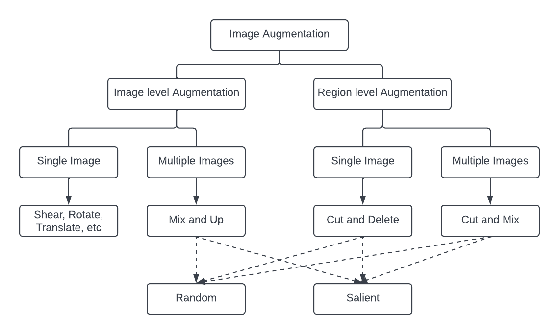
Figure 1: The categorization of image mixing and deleting data augmentation techniques. The three main types are Cut $\&$ Delete, Cut $\&$ Mix and Mix $\&$ Up.

1 Introduction

“Where there is ruin, there is hope for a treasure.” - Rumi

Deep Neural Networks have shown tremendous success in image classification [80, 49], object detection [78, 77], and semantic segmentation [9, 111]. These networks are data hungry with millions of parameters that make them prone to overfitting [57, 104, 73]. To enhance model generalization, many approaches have been suggested, for example, regularization [56], dropout [86], and data augmentation [83]. The purpose of data augmentation is to increase the dataset size by introducing various corruptions in the data so that the model does not memorize the irrelevant patterns in the data. Conventional image augmentations include image rotation, random cropping, jittering, translation, shear, solarize, posterize, brightness, etc. In addition to these techniques, a relatively new data augmentation strategy mixes and deletes different image regions. The augmented images generated by this approach are present in the vicinity of the original data distribution. The model trained with this new data generalizes well against data variations, avoids overfitting, and achieves robustness against data corruption. The benefits of image mixing and deleting are label smoothing, robustness to occlusions, noise, image corruptions, and adversarial examples, improved classifier calibration, consistency, and out-of-distribution data predictions. Overall, the model learns to focus on the complete structure of the object under consideration resulting in improved performance.

Image mixing and deleting can be divided into three main categories: 1) cut and delete 2) cut and mix, and 3) mix and up. Figure 1 shows the taxonomy of image augmentation. Cut and delete [20, 50, 10, 113] erases the selected region, cut and mix [105, 98, 91, 76, 95, 39] replaces the selected area with some part of another image, whereas mix and up [106, 97, 53, 45, 42] mixes the pixel intensity values of two or more images. The first two categories are region-level augmentation, while the third category is image-level augmentation. Within these categories, many approaches rely entirely on random data augmentation strategies. In contrast, others consider salient information either keeping it or deleting it in the generated image.

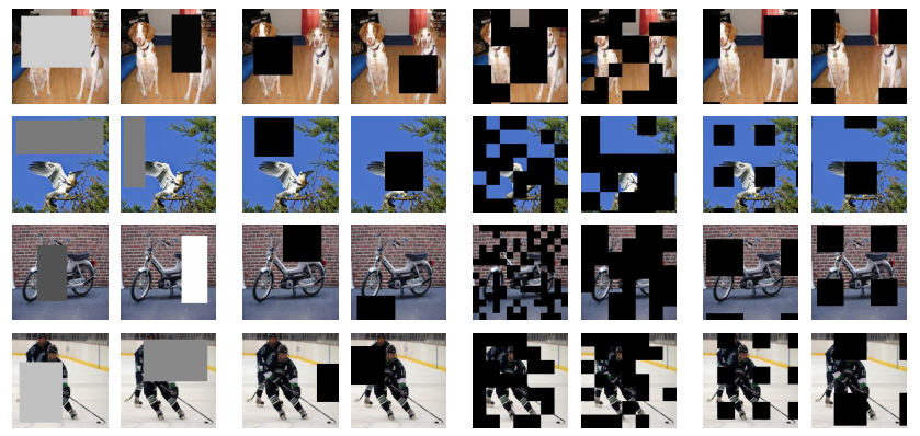
Figure 2: Comparison of various cut and delete strategies, CutOut (Columns 1, 2), Random Erasing (Columns 3, 4), hide $\&$ seek (Columns 5, 6), and GridMask in the last two columns (image is taken from [10]).

Although image mixing and deleting improves the overall performance by adding noise and ambiguity in training data and labels, it is also likely to reduce the model accuracy if performed naively. Therefore, carefully performing image mixing and deleting is essential as it should not reduce or delete the information in an image beyond a specific limit, or the model will not have sufficient information to learn and distinguish between classes. Extreme levels of changes in an image can make the label irrelevant and noisy for the model. To avoid this situation, many approaches suggested in the literature [27, 98, 46, 45] emphasize on retaining salient information in the augmented images.

The generalization power of image mixing and deleting is not only limited to image classification. It has also been proven to increase accuracy for fine-grained image recognition and object detection tasks. The trained model employing suggested augmentation approaches can replace the object detection backbones, or object detection training can incorporate these augmentations; both training methods have been shown to improve accuracy over the baseline models. For fine-grained image recognition, particular augmentation strategies by image mixing are proposed. Apart from this, image mixing or deleting can efficiently be utilized along with regularization [56], dropout [86], or conventional image augmentations [83] based on affine transformations, to further enhance the model performance.

This review is focused entirely on the proposed image mixing and deleting data augmentation techniques. It does not discuss any approaches that augment data using multiple geometric and color transformations [17] or perform neural augmentation search [16, 62]. A review of various geometric and color augmentations is available in [83, 43]. Moreover, we organize the image mixing and deleting-based augmentation schemes into three main categories including 1) erasing image patches, 2) cutting the image region and replacing it with some other image region, and 3) mixing pixel values of multiple images. The following sections discuss all proposed approaches within these categories in detail.

2 Cut and Delete

This section discusses data augmentation by deleting image patches randomly or semantically. The purpose of erasing image patches is to allow the network to learn in case of occlusions. This way, the model is forced to understand and focus on partially visible object properties. This kind of dropout is different from conventional dropout because it drops contiguous image regions, whereas values in traditional dropout work at non-contiguous locations. Here, much of the image region is provided to the network to build connections semantically among various parts of the image. Below, we would like to discuss the approaches that fall into this category.

2.1 Cutout

Cutout [20] removes constant-size square patches randomly by replacing them with any constant value. Region selection is performed by selecting a pixel location randomly and placing a square around it. In this procedure, Cutout region lying outside the borders is allowed and proven to improve performance. Patch deletion is applied on all the training images where the optimal patch size is a hyperparameter selected by performing a grid search on training data. An example is shown in Figure 2.

2.2 Random Erasing

Random Erasing [113] deletes contiguous rectangular image regions similar to Cutout [20] with minor differences in the region selection procedure. Contrary to Cutout [20], where deletion is applied on all the images, random erasing is performed with a probability of 0.5. In every iteration, region size is defined randomly with upper and lower limits on the region area and aspect ratio. The algorithm ensures erasing region stays inside the image boundaries, as opposed to Cutout. Moreover, random erasing provides region-aware deletion for object detection and person identification tasks. Regions inside the object-bounding boxes are randomly erased to generate occlusions. Figure 2 shows some augmented images.

2.3 Hide and Seek

Hide and Seek [50] divides an image into a specified number of grids and turns each grid cell on or off with an assigned probability. This way, random small image regions that may be connected or disconnected from each other are deleted (see Figure 2). The grid cells that are turned off are replaced with the average of all the pixel values in the entire dataset.

2.4 GridMask

Another simple approach is GridMask [10], where the algorithm tries to overcome the drawbacks of Cutout, Random Erasing, and Hide $\&$ Seek, which are prone to deleting important information entirely or leaving it untouched without making it harder for the algorithm to learn. To handle this, the GridMask [10] creates multiple blacked-out regions in evenly spaced grids to maintain a balance between deletion and retention of critical information. The number of masking grids and their sizes are tuneable. The article also compares erasing a single region vs. multiple regions, showing that GridMask is less likely to hide out foreground information completely. Even with the large box size, it retains a sufficient amount of important information for the model to learn. GridMask-generated examples are shown in Figure 2.

2.5 Cut and Delete for Object Detection

This section describes Cut and Delete, designed explicitly for object detection.

Adversarial Spatial Dropout for Occlusion [100] drops region pixels to generate hard positives for object detection by learning key image regions. Within the proposed region, only 1/3 of pixels are dropped after sorting based on magnitudes in the heatmap. A separate network learns the salient image regions. The mask generator is penalized based on the detector’s performance, similar to generative adversarial networks [28].

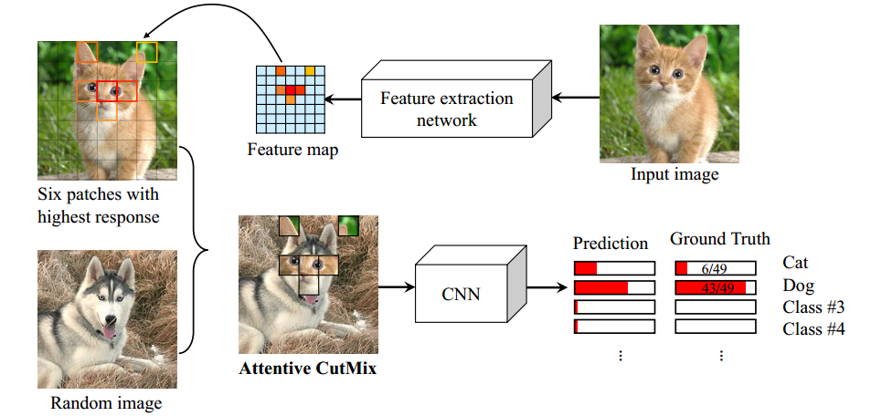
Figure 3: The Attentive CutMix image augmentation procedure, attentive regions from one image are overlayed on another image, image is taken from [98].

3 Cut and Mix

Instead of deleting a patch, Cut and Mix replaces the patch with another image region. Thus, the image shares information coming from multiple class labels, however, the significant class label belongs to the original class label. Hence, the model learns to differentiate between two classes within a single image. This method of augmentation introduces label smoothing as a by-product.

3.1 CutMix

In CutMix [105], images are augmented by sampling patch coordinates, $x,y,h,w$ from a uniform distribution. The selected patch is replaced at the corresponding location with a patch from the other randomly picked image from the current mini-batch during training. CutMix [105] updates the image labels proportion to the replaced patch as defined in the Eq. 1, where $M$ is the image mask, $x_{a}$ and $x_{b}$ are images, $\lambda$ is the proportion of label, and $y_{a}$ and $y_{b}$ are the labels of images.

$$x_{new}=M.x_{a}+(1-M).x_{b}$$ (1)

$$y_{new}=\lambda.y_{a}+(1-\lambda).y_{b}$$

3.2 Attentive CutMix

Attentive CutMix [98] builds up on CutMix. Instead of random pasting, it identifies attentive patches and pastes them at the exact location in the other image. This avoids the problem of selecting a background region that is not important for the network and updating the label information accordingly, as in Eq. 1. A separate pre-trained network is employed to extract attentive regions. The attention output is mapped back onto the original image. The image is divided into a grid of patches, where six highly activated responses are pasted onto the training image as demonstrated in Figure 7. These image pairs are selected randomly in every training iteration. The flow diagram of Attentive CutMix is shown in Figure 3.

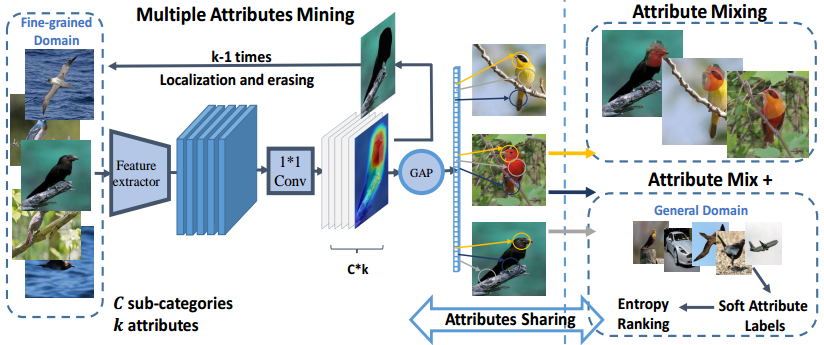
Figure 4: An example of attribute mining and mixing procedure. (image is from [58])

3.3 RICAP

Random image cropping and patching (RICAP) [91] performs data augmentation by cropping four random regions from four sampled images and combining them to create a new image. The generated image has mixed labels proportional to the pasted area. The area of cropped regions in the output image is determined by sampling through uniform distribution. The authors RICAP [91] suggest three methods for common boundary points in the augmented image: anywhere-RICAP (origin can be anywhere), center-RICAP (origin can only be in the middle of the image), and corner-RICAP (origin can only be in corners). Corner-RICAP has shown the best performance due to a larger region of one image being visible to the network to learn.

3.4 Mixed Example

This method [87] experimented with 14 different types of augmentation approaches. The output image is generated using the following techniques: vertical concatenation, horizontal concatenation, mixed concatenation, random 2$\times$2, VH-mixup (vertical concatenation, horizontal concatenation, and mixup), VH-BC+ (vertical concatenation, horizontal concatenation, and between-class), random square, random column interval, random row interval, random rows, random columns, random pixels, random elements, and noisy mixup. From all these approaches, VHmixup has the best performance.

3.5 CowMask

CowMask [26] is used in semi-supervised learning where original and augmented images are brought closer during training. CowMask suggests two types of mixing approaches 1) erasing and 2) mixing two images similar to CutMix. This technique’s mask is irregular rather than rectangular, generated by applying a Gaussian filter (scale $\sigma$) on a normally distributed noise image. A suitable threshold is selected to ensure a proportion $p$ of non-masked image pixels are present in the output image. Pixel values below the threshold are either erased or replaced by the pixel values of the noise image at the corresponding locations.

A very similar masking approach for data augmentation is FMix [33] which uses the inverse Fourier transform of a noise image to generate binary masks containing top $\lambda wh$ pixels with 1 values.

3.6 ResizeMix

ResizeMix [76] performs random image cropping and pasting. It empirically proves to perform better than salient and other non-salient image mixing methods, as shown in Table 4. ResizeMix solves the random region cropping problem that misallocates the output image label in some instances where the pasted region does not contain any object information. The labels of the output image are updated as per Eq. 1. ResizeMix handles this by completely scaling down (scale rate is sampled from a uniform distribution) the selected image and pasting it randomly on the target image, as shown in Figure 7.

3.7 SaliencyMix

Instead of random Cut and Mix, SaliencyMix [95] extracts the salient region and pastes them on the corresponding location in the target image. The salient region is extracted around the maximum intensity pixel location in the saliency map. Augmented image labels are updated as per Eq. 1.

3.8 KeepAugment

Similar to SaliencyMix [95] and Attentive CutMix [98], KeepAugment [27] performs augmentation based on the salient region. However, this approach uses one image for the augmentation. KeepAugment identifies the salient area in an image and ensures that the image generated by the augmentation strategies, for example, Cutout [20], randaugment [17], CutMix [105] or autoaugment [16], contains the salient region in it.

3.9 RecursiveMix

RecursiveMix [103] iteratively mixes images from the previous iteration into the current iteration. Similar to ResizeMix [76], it resizes and pastes the mixing image on top of the input image but employs previously generated output (containing multiple classes), mixing recursively while maintaining the history of one mini-batch. Labels of the generated image have class values proportional to the amount of the region. The network is trained with classification and consistency loss to learn semantic representations in multi-scale and spatial-variant views, as given in Eq. 2

$$L=L_{CE}(x_{m},y_{m})+\omega\lambda L_{KL}(p_{roi},p^{h}),$$ (2)

where $CE$ is cross-entropy loss, $x_{m}$ and $y_{m}$ are the mixed image and label, respectively, $\omega$ is the consistency loss weight, $\lambda$ is the image mixing ratio, $KL$ is the Kullback Leibler Divergence, $p_{roi}$ is the network’s prediction for the resized smaller pasted image on the input image, whose features are extracted and aligned by $roi$, i.e., RoIAlign operator [34], and $p^{h}$ is the network’s prediction for the historical image. The KL divergence minimizes the model’s prediction variance between the historical and generated images. Examples of the RecursiveMix generated images are shown in Figure 7.

3.10 LUMix

LUMix [89] corrects the label misallocation of CutMix, perturbing the labels by adding noise and reducing the input class label value if the output image does not contain the class information. The label equation in Eq. 1 updates to the following:

$$\lambda=(1-r_{1}-r_{2})\lambda_{0}+r_{1}\lambda_{r}+r_{2}\lambda_{s},$$ (3)

where $r_{1}$ and $r_{2}$ are the hyper-parameters, $\lambda_{0}$ is the CutMix $\lambda$ as in Eq. 1, $\lambda_{r}$ is a random value drawn from the Beta distribution, and $\lambda_{s}$ is calculated in Eq. 4 using the network’s predictions on the CutMix input image.

$$\lambda_{s}=\frac{p_{y_{a}}}{p_{y_{a}}+p_{y_{b}}}.$$ (4)

In the above Eq., $p_{y_{a}}$ and $p_{y_{b}}$ are the predicted probabilities for the $y_{a}$ and $y_{b}$ classes, respectively. The $\lambda$ in Eq. 4 updates labels in Eq. 1, later used for backpropagation. The lower value of $p_{y_{a}}$ decreases the $\lambda$ value, which in turn reduces the penalization for the $y_{a}$ class, suggesting the absence of input class information.

3.11 Saliency Grafting

Saliency Grafting [74] incorporates salient information for both the image and label mixing. Instead of pasting the most salient patches from the random image, Saliency Grafting selects patches randomly using a 2D-Bernoulli distribution. The labels are modified based on the amount of salient information of both images present in the output image. The following Eq. 5 describes the label-mixing procedure:

$$y=\lambda(S_{a},S_{b},M)y_{a}+(1-\lambda(S_{a},S_{b},M))y_{b},$$ (5)

where $\lambda=\frac{I(S_{a},M)}{I(S_{a},M)+I(S_{b},1-M)}$ and $I=\frac{||S\circ M||_{2}}{||S||_{2}}$. Moreover, $S$ is the attention map, $M$ is the mask, $I$ is the salient information present in the output image, $\lambda$ is the hyper-parameter and $y$, $y_{a}$, and $y_{b}$ are the image labels. See examples of the Saliency Grafting augmented images in Figure 7.

3.12 Fine-Grained Image Recognition

Attribute Mix [58] augments images based on semantically extracted image attributes. It trains an attribute classifier by extracting $k$ attributes (e.g., leg, head, and wings of a bird) from each image. The attribute mining procedure for every image is performed $k$ times repetitively. For each iteration, an attribute is masked out from the original image based on the most discriminative region in the attention map. With these images, an attribute-level classifier is trained to generate new images for the actual classification model. For the given two images, the attribute-level classifier identifies attribute masks; these masks are randomly picked to create a new training image. The procedure of label update is the same as in Eq. 1. The attribute mining and attribute mixing process can be seen in Figure 4.

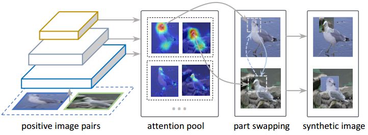
Figure 5: Architecture of the Intra-class part swapping. The figure is from [109].

Intra-Class Part Swapping [109] replaces the most attentive regions, extracted using a classification activation map (CAM) thresholded for the most prominent region, of one image with another. The attentive region in the source image is scaled and translated according to the attentive region of the target image for region replacement. The label information of the output is similar to the target image as this approach relies on augmenting similar class images. Figure 5 presents the architecture of intra-class part swapping.

SnapMix [39] augments training images by extracting and merging random image regions of different sizes, where the region size for both images is drawn through the beta distribution. Generated image label is assigned based on semantic composition from normalized (sum to one) CAMs. Figure 6 illustrates an example of image augmentation. The procedure of label generation is similar to Eq. 1. However, the summation of label coefficients can exceed one depending on the semantic composition of the output image.

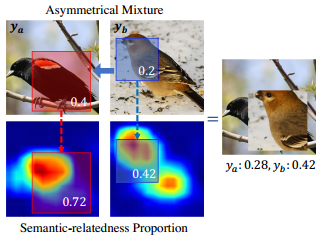
Figure 6: Example of SnapMix taken from [39]

3.13 Cut and Mix for Transformers

TransMix [8] employs Vision Transformers (ViTs) [21] to identify attentive regions taken from the random image in CutMix generated image. These attentive regions are used to update labels ($\lambda$ in Eq. 1) based on the information present in the output image.

TokenMix [66] splits the mask into multiple patches, where patches are on and off at distributed locations instead of one large rectangular region, as in CutMix. The labels are updated according to the attentive regions CutMix in the output image.

3.14 Cut and Mix for Object Detection

This section discusses Cut and Mix approaches specifically designed for object detection.

Visual Context Augmentation [23]. This augmentation strategy learns to place object instances at an image location depending on the surrounding context. A neural network is trained for this purpose. The training data is prepared to generate a context image with the masked-out object inside it. From an image, 200 context sub-images are generated surrounding the blacked-out bounding box. The neural network learns to predict the category (object or background) in masked pixels. During testing, the context network identifies plausible object bounding boxes. The object instances are placed inside the selected boxes to generate a new training image. These newly created images are used as training data for the other network, for example, object detectors.

Cut, Paste and Learn  [24]. This simple approach generates new data by extracting object instances and pasting them on randomly selected background images. Instances are blended with various blending approaches, for example, Gaussian blurring and Poison blending, to reduce pixel artifacts around the augmented object boundaries. Added instances are also rotated, occluded, and truncated to make the learning algorithm robust. This simple data mixing approach improves object detection performance.

	Random Images				Input Image
CutMix
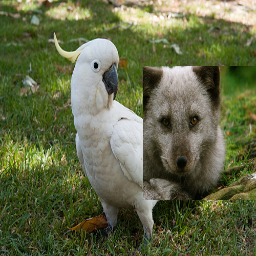
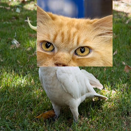
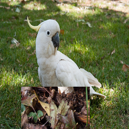
Att. CutMix
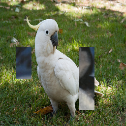
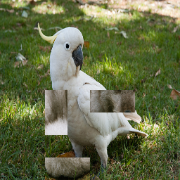
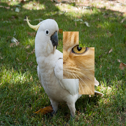
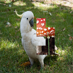
CowMask
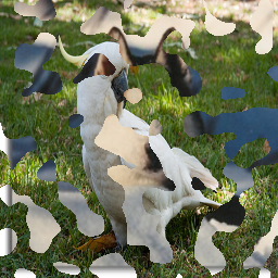
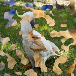
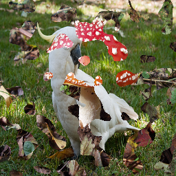
ResizeMix
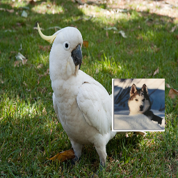
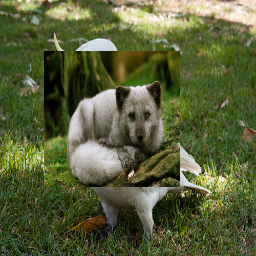
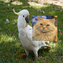
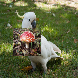
KeepAug.
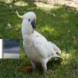
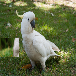
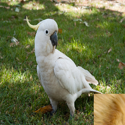
SaliencyMix
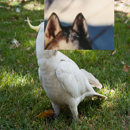
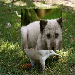
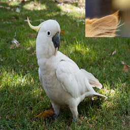
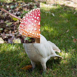
RecursiveMix
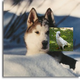
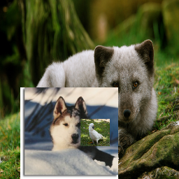
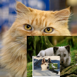
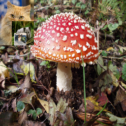
SaliencyG.

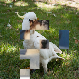
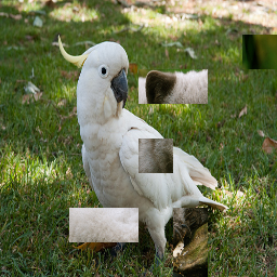
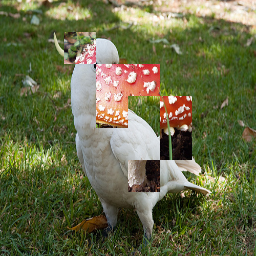
Figure 7: A comparison of various cut and mix approaches. The topmost row shows original images, while the other rows are augmented images. SaliencyG. refers to Saliency Grafting [74].

4 Mix and Up

This type of data mixing is different from Cutout and CutMix, in the sense that it mixes pixel values of two images instead of cropping or erasing image regions. Mix and Up regularizes neural networks by forcing them to learn linear interpolations between training images. The network trained with Mix and Up has shown robustness to adversarial attacks with improved performance on the test set.

4.1 MixUp

MixUp [106] generates a new image by mixing pixel values of two randomly selected images. The mixing factor decides the proportion of pixel strength during data mixing $\lambda$ $\in$ [0-1] as shown in Eq. 6. The values for $\lambda$ are drawn from the beta distribution.

$$x_{new}=\lambda.x_{a}+(1-\lambda).x_{b}$$ (6)

$$y_{new}=\lambda.y_{a}+(1-\lambda).y_{b}.$$

RegMixUp [75] employs MixUp as a regularizer along with the standard cross-entropy loss.

4.2 Manifold MixUp

Different from MixUp, Manifold MixUp [97] mixes feature values generated from intermediate neural network layers. For two random images, inputs are fed forward up to the $k$ layer of the network, where the output feature maps are mixed based on Eq. 6. The mixed feature maps are inputted to the next layer and forward propagated up to the last layer. Finally, backward propagation is performed in the standard way with updated labels (similar to MixUp).

Noisy Feature MixUp [63]. This method injects additive and multiplicative noise into the Manifold MixUp output. Eq. 6 for Noisy Feature MixUp becomes:

$$x_{new}=(1+\sigma_{1}\xi_{1})(\lambda.x_{a}+(1-\lambda).x_{b})+\sigma_{2}\xi_{2},$$ (7)

where $\sigma$ is a scalar, and $\xi$ is drawn from a probability distribution (Gaussian) and has the same dimension as the mixing output image.

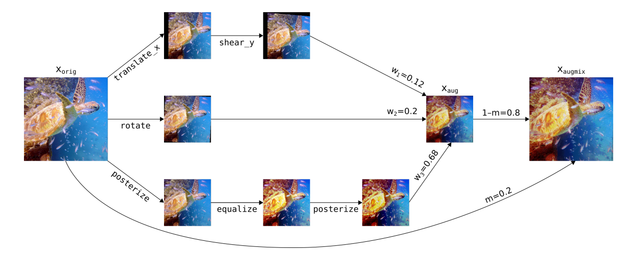
Figure 8: AugMix [36] data augmentation procedure. Multiple transformations are applied randomly on the image in separate branches that are later combined to generate one image. Example taken from [36].

4.3 AugMix

	Input Images				Random Image
MixUp
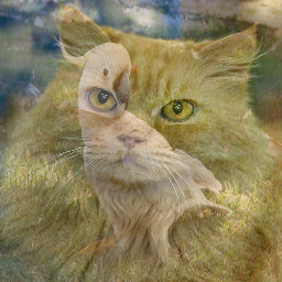
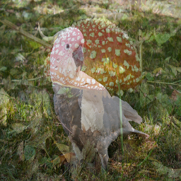
AugMix
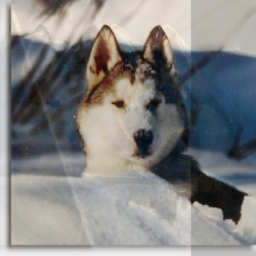
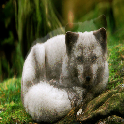
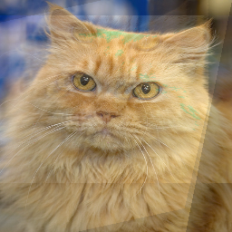
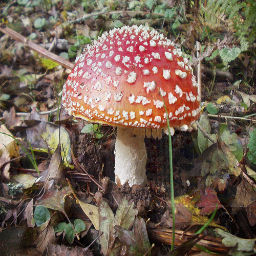
SmoothMix
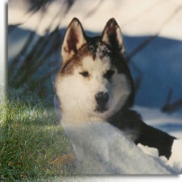
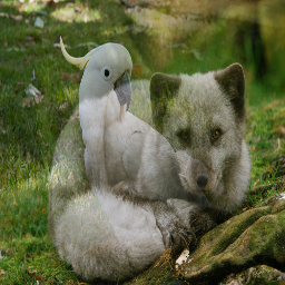
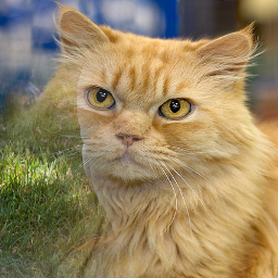
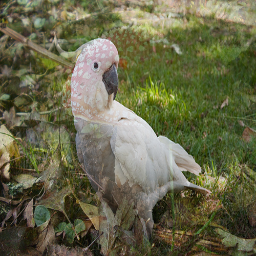
Co-MixUp
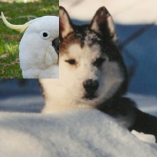
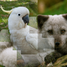
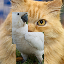
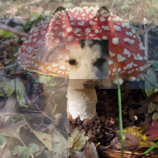
Puzzle Mix
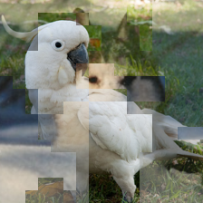
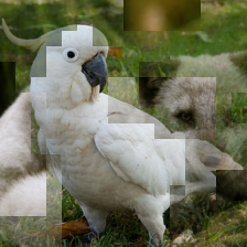
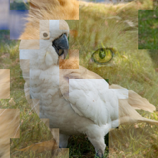
SuperMix
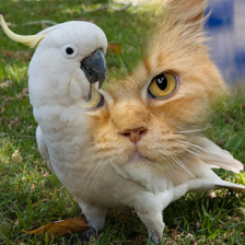
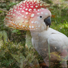
PixMix

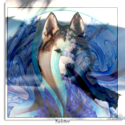
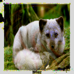
Figure 15: A comparison of various MixUp techniques. The topmost row shows original images, whereas other rows are augmented images.

AugMix [36] performs data mixing using the input image itself. It transforms (translate, shear, rotate, etc.) the input image and mixes it with the original image. Image transformation involves a series of randomly selected augmentation operations applied with three parallel augmentation chains. Each chain has a composition of functions that could include employing, for example, translation on input image followed by shear, etc.. The output of these three chains is three images mixed to form a new image (see Figure 8). This new image is later mixed with the original image to generate the final augmented output image, as per Eq. 6. The transformations in AugMix [36] are selected from autoaugment [16]. A comparison of AugMix [36] augmented images with other methodologies is given in Figure 15.

Figure 9: An example of network training via SmoothMix strategy, where the figure is from [53].

4.4 SmoothMix

SmoothMix [53] is a mask-based approach matching closely with the Cutout and CutMix techniques. However, it has a few differences: 1) the mask has soft edges with gradually decreasing intensity, and 2) the mixing strategy is the same as in Eq. 6. The augmented image has mixed pixel values depending on the strength of the mask, as shown in Figure 9. The authors suggest various square and circular masks containing smooth edges. From these, circular masks generated using Gaussian distribution perform better. The following decides the value of $\lambda$.

$$\lambda=\frac{\sum_{i=1}^{W}\sum_{j=1}^{H}G_{ij}}{WH},$$ (8)

where $G_{ij}$ is the pixel value of mask $G$, $H$ is height, and $W$ is width. With the given mask, the equation to mix two images becomes

$$x_{new}=G.x_{a}+(1-G).x_{b}$$ (9)

$$y_{new}=\lambda.y_{a}+(1-\lambda).y_{b}.$$

4.5 Co-Mixup

Co-Mixup [45] performs salient image mixing on a batch of input images to generate a batch of augmented images. This technique maximizes saliency in output images by penalizations to ensure local data smoothness and diverse image regions. Examples of generated images by Co-Mixup are shown in Figure 15.

4.6 Sample Pairing

This technique [42] merges two images by averaging their pixel intensities. The resultant image has the same training image label as opposed to MixUp and other approaches where labels are updated according to the proportion of image mixing.

4.7 Puzzle Mix

Puzzle Mix [46], as shown in Figure 15, learns to augment two images optimally based on saliency. The algorithm employs the following procedure 1) images are divided into regions for the MixUp, and 2) the algorithm learns to transport the salient region of one image such that the output image has the maximized saliency from both images.

4.8 SuperMix

SuperMix [19] performs MixUp [106] on multiple images. It mixes salient information extracted using a set of mixing masks $M=\{m_{i}\}_{i=0}^{k}$. These masks are optimized to generate an output image that contains the label information equivalent to the predictions of a teacher model, given below:

$$\hat{x}=\sum_{i=0}^{k-1}m_{i}x_{i}\quad\text{and}\quad\hat{y}=\sum_{i=0}^{k-1}r_{i}\delta(y^{T}(x_{i})),$$ (10)

where $k$, $r$, $\delta$, and $y^{T}(x_{i})$ are the mixing size, random sample from Dirichlet distribution, one hot encoding, and the teacher network prediction for the $ith$ image, respectively. The masks are optimized by minimizing the KL divergence between the teacher network predictions for the mixed image and the labels (from Eq. 10) defined as

$$\underset{i=0,...,k-1}{min}\ KL(f^{T}(\hat{x})\parallel\hat{y})+\lambda_{\sigma}L_{\sigma}(m_{i})+\lambda_{s}L_{s}(m_{i}).$$ (11)

Here, $f^{T}$ is the teacher network, $\lambda_{\sigma}$ $\&$ $\lambda_{s}$ are hyper-parameters, $L_{\sigma}$ is the total variation norm to penalize mask roughness, and $L_{s}$ encourages the network to have mask values approaching to 0 or 1, where $L_{s}=\frac{1}{kWH}\sum_{i}m_{i}(m_{i}-1)$. Figure 10 illustrates this optimization process and the classification model that uses the resultant output image from the optimization process for training; examples are shown in Figure 15.

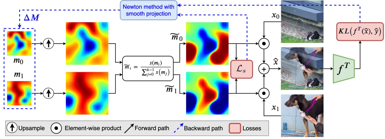
Figure 10: SuperMix augmented image generation process, the figure is taken from [19].

4.9 AutoMix

AutoMix [67] employs a mix block network to generate image mixing masks to avoid label mismatch in MixUp. Mix block is a cross-attention module that takes mixing images feature maps as input, extracted from a momentum encoder. Mix block, momentum encoder, and the classification model are trained end-to-end with a momentum pipeline, where the momentum encoder is the exponential moving average of the classification model. The complete training pipeline is visible in Figure 11. A joint loss, given in Eq. 12, is optimized during the training process.

$$l_{\lambda}=\gamma max( ||\lambda-\frac{1}{HW}\sum_{h,w}{s_{a}}||-\epsilon,0)$$ (12)

$$L =l_{ce}+l_{\lambda}.$$

In the above Eq., $l_{\lambda}$ is the mix block loss, $\gamma$, $\lambda$, $\epsilon$ are hyper-parameters, $s_{a}$ is the mask for the $x_{a}$ image, $l_{ce}$ is the classification and mask generation cross-entropy loss, and $L$ is the combined loss.

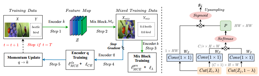
Figure 11: AutoMix image mixing and training procedure, the figure is taken from [67].

4.10 ReMix

ReMix [15] addresses the issue of class imbalance by generating mixed images for minority classes. The process of remixing is identical to Eq. 6 for data mixing. However, in the case of label assignment, it sets the label of the output image to the minority class.

4.11 PixMix

PixMix [37] improves the model performance in various dimensions, robustness, consistency, calibration, corruption, adversarial, and anomaly detection while maintaining an excellent comparable accuracy to other methods on a clean dataset. The mixing procedure employs fractals and feature map visualizations to mix with the input image, rather than some random dataset image as in other Mix $\&$ Up methods, depicted in Figure 12. The input image is augmented $k$ times, either by addition or multiplication. Within these augmentation rounds, input image mixes with fractals, feature map visualizations, and augmented (rotated, posterized, solarized, etc.) versions of the original image.

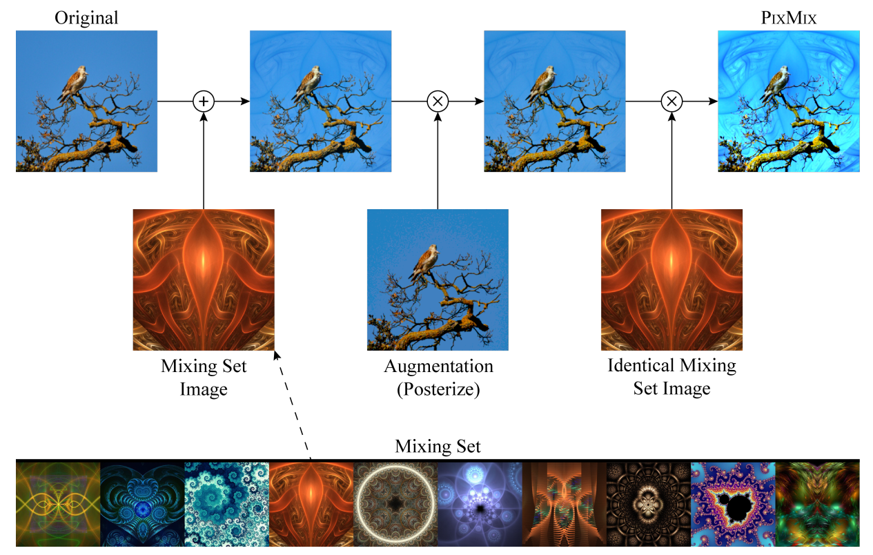
Figure 12: Image augmentation strategy of PixMix. The bottom row shows the mixing set fractals, where the image is taken from [37].

4.12 StyleMix

StyleMix [38] generates new images by mixing style and content from image mixing pairs; an example is available in Figure 13. The style of one image is transferred to another using adaptive instance normalization [40] on encoded feature vectors. Lets consider two images $x_{1}$ and $x_{2}$, their encoded and adaptive instance normalized [40] feature vectors are following:

$$f_{11} =f(x_{1})$$ (13)

$$f_{22} =f(x_{2})$$

$$f_{12} =AdaIN(f_{11},f_{22})$$

$$f_{21} =AdaIN(f_{22},f_{11}),$$

where $f$ is a VGG network up to the first few layers. The $AdaIN(f_{12},f_{21})$ is from [40] and given by:

$$AdaIN(f_{ii},f_{jj})=\sigma(f_{ii})\frac{f_{ii}-\mu(f_{ii})}{\sigma(f_{ii})}+\mu(f_{jj}).$$ (14)

The mean $\mu$ and variance $\sigma$ are computed individually for each channel. The mixed image and its label are generated by Eq. 15 below.

$$x_{m} =g(tf_{11}+(1-r_{c}-r_{s}+t)f_{22}$$ (15)

$$+(r_{c}-t)f_{12}+(r_{s}-t)f_{21})),$$

$$y_{m} =ry_{c}+(1-r)y_{s},$$

$$y_{c} =r_{c}y_{1}+(1-r_{c})y_{2},$$

$$y_{s} =r_{s}y_{1}+(1-r_{s})y_{2},$$

where $r_{c}$ and $r_{s}$ are content and style parameters, respectively. The interpolated image $x_{m}$ contains $r_{c}$ content of $x_{1}$ ($1-r_{c}$ of $x_{2}$) and $r_{s}$ style of $x_{2}$ ($1-r_{s}$ of $x_{1}$), whereas $t$ is a free parameter within the range $max(0,r_{c}+r_{s}-1)\leq t\leq min(r_{c},r_{s})$.

In addition to MixUp-based style mixing, StyleMix also suggests StyleCutMix, where the output image has the styles either from the cut-pasted region of the random image or the original image depending on the parameters in Eq. 15.

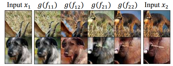
Figure 13: A pre-trained encoder and decoder generate StyleMix images. We can observe that $g(f_{11})$ has the content and style of $x_{1}$. Similarly, $g(f_{12})$ contains content of $x_{1}$ and style of $x_{2}$ and so on. Image is from [38].

4.13 AlignMixUp

AlignMixUp [96] geometrically aligns and interpolates two images in the feature space. The reconstruction of aligned-mixup feature space displays the content of one image and the texture of the other; an example is shown in Figure 14. AlignMixUp uses sinkhorn [18] algorithm to align features, and MixUp with interpolating original and aligned feature spaces of two images.

4.14 Mix and Up for Transformers

TokenMixup [14]. In this method, images in a mini-batch are paired optimally to increase salient information in the output. TokenMixup calculates the saliency score for each token using the transformer’s multi-head attention layer. The difference in these scores between all the mini-batch images is calculated and provided to the Hungarian matching algorithm to generate optimal image pairs for maximum saliency. An image pair’s less salient image tokens are mixed with the salient tokens. Before applying this process, TokenMixup identifies the hard images using an auxiliary classifier and skips them from the mixing procedure. Likewise to the other saliency-based image mixing methods, the augmented image labels are based on the salient information present in the output.

4.15 Mix and Up for Object Detection

Similar to Cutout and CutMix, MixUp is also used to enhance the performance of object detection algorithms. One of the approaches in [5] MixUp image data to update object labels and locations. Instead of employing the basic MixUp strategy, this algorithm identifies object locations, mixes object pixels at corresponding locations in two images, and updates the object box coordinates in the output image depending on the prominent object and the image label.

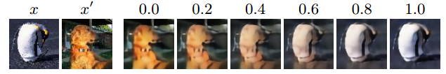
Figure 14: An example of AlignMixUp from [96] shows interpolated and aligned images generated through the decoder. The mixing ratio values $[0,1]$ are shown with their effects on the output image.

5 How does Image Mixing and Deleting improve network training?

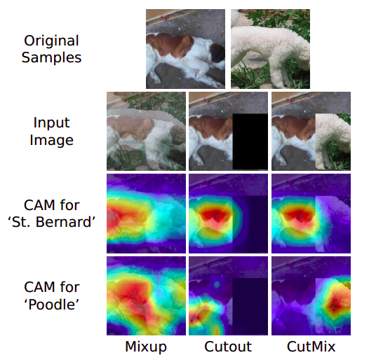
Figure 16: Class Activation Maps (CAMs) for the augmented images, which are taken from [105].

Understanding the underlying cause of why these techniques improve baselines’ performance is important. This builds the foundation to improve the existing approaches. Various methods are adopted to analyze standard training procedures and training with augmentations. Cutout [20] and CutMix [105] argue that hindering image regions drives the classifier to learn from the partially visible objects and understand the overall structure. CutMix verifies this argument by showing enhanced focus toward the target class in CAMs, shown in Figure 16.

In contrast, MixUp has been shown to improve the classifier’s calibration and reduce prediction uncertainty in [93]. To demonstrate this, the authors compared the mean of predictions against accuracy, where the confidence distribution for the MixUp trained model is evenly distributed against the standard model whose distribution is towards higher confidence, i.e., over-confidence. Similarly, the loss contours obtained for a network trained with MixUp are smooth compared to sharp contours in standard training [61]. A few theoretical discussions [108, 6] show multiple regularization effects to the standard loss with MixUp training using Taylor series approximation. MixUp introduces various regularization effects like label smoothing, Jacobian regularization, minimizing an upper bound of the adversarial loss [108], etc. Training with MixUp is equivalent to learning with structured noise in the data [6]. All these theoretical and practical justifications [93, 61, 108, 6] establish better generalization and robustness against noise by MixUp training.

Strengths and Weaknesses The objective of the image augmentation methods is regularization, introducing diversity in training data, and achieving robustness to occlusions and object shape changes. Augmentation methods like CutMix and MixUp add the benefit of label smoothing, whereas the additional advantage of MixUp is robustness to image noise. The benefits mentioned are common to each technique. Here, we provide the strengths and weaknesses of the augmentation methods in Tables 1, 2 and 3 for each approach.

Table 1: The strengths and weaknesses of cut and delete approaches for image classification.

Method	Strengths	Weaknesses
CutOut	Strengthen activations and increases their count, enforce the network to consider diverse features in making predictions, and avoid over-fitting	Hiding regions randomly can lead to erasing important regions
Random Erasing	Similar benefits as cutout. Extends the experimentation to object detection and shows the benefits of random erasing like regularization, robustness to occlusions, etc	Hiding regions randomly can lead to erasing important regions
Hide and Seek	Similar benefits as above. Erases multiple patches to make the network robust to occlusions	Severe under-fitting if too many object patches are hidden
GridMask	Multiple patches are deleted with even spacing between them to retain a balance of deletion and retention of object information	Under-fitting if too many object patches are hidden

Table 2: The Strengths and weaknesses of the Cut and Mix augmentation types for image classification.

Method	Strengths	Weaknesses
CutMix	Opposite to cutout, cutmix pastes a region from another image along with a label value proportional to the region that apparently fixes label corruption in cutout	Label corruption is possible if an important region is replaced or the background region is pasted in the original image. This ends up with the absence of object in the image but containing the label value of the object
Attentive CutMix	Only attentive regions in the second image are cutmix at the same location as the original image	Extracting attentive regions is slow as compared to random selection. Attentive regions of the original image are not considered during replacement, this can corrupt label
RICAP	Increased label smoothing effect as it creates an augmented image by patching four random regions from four different images with label proportion to the regions	Label corruption is possible because of background information
Mixed Example	Suggested 14 different linear and non-linear (vertical- concat, vertical-horizontal mixup, etc) augmentations	Only a few of the augmentation methods have better performance than the baseline. No performance comparison was performed with the combination of multiple augmentation methods
CowMask	Irregular-shaped mask similar to Friesian cow skin patterns is used instead of rectangular shape. These masks reduce the chances of removing consecutive key regions and introduce more diversity in augmented image	Gaussian filtering is required to generate masks. Blacking out too many image areas can cause severe under-fitting, therefore a balance of data deletion and retention is important
ResizeMix	It handles label misallocation by resizing and pasting the complete object on the target image randomly	Label corruption due to background pasting of source image is managed but it is possible to hide key areas of the target image due to random pasting
SaliencyMix	The highly attentive region from the source image is pasted on the target image to avoid label corruption	Because the attentive region from the source image is pasted at the corresponding location in the target image, therefore it occludes the target image object for some of the training data
KeepAugment	This method retains salient region information of the target image in augmented image	In keepcutout and keepcutmix, source image regions are deleted or pasted randomly which can lead to label misallocation
RecursiveMix	This method has enhanced CAMs visualization and learns better representations with the consistency loss	In addition to ResizeMix weaknesses, RecursiveMix requires storage to maintain the history for image mixing and computation, i.e., RoIAlign for consistency loss
LUMix	Reduces label misallocation in CutMix	-
Saliency Grafting	Mixes images and labels based on salient information with random salient patch selection to increase sample diversity	Additional compute for saliency calculation

Table 3: The strengths and weaknesses of image classification data augmentation approaches of Mix and UP.

Method	Strengths	Weaknesses
MixUp	Additional to regularization and label smoothing, mixup introduces adversarial robustness	The advantages of mixup are unknown to image segmentation. Overlapping objects in mixup images can corrupt labels but not as severe as cutmix
Manifold MixUp	Applying mixup at hidden layers rather than at the input generates tighter class representations, generalizes better to novel deformations not seen during training	Because intermediate representations are used for the mixup, visualizing and explaining changes in the augmented data like other augmentation methods is not possible.
AugMix	Preserves image semantics, creates a model that is robust to corruptions and data shifts and improves calibration metrics. No possibility of label misallocation	Unknown
SmoothMix	Mixup images smoothly using a soft edge mask to avoid sharp changes in pixel values	Same as mixup
Co-Mixup	Extended mixup to multiple images, maximizes saliency in the augmented image, increases smoothness in mixed data	Additional compute cost to extract saliency information. The output image has broken structures sometimes
Sample Pairing	No additional strengths	Averages pixel intensities and labels of two images without any diversity in generating data
Puzzle Mix	Maximizes salient information in generated image, creates smooth images and preserves local data statistics	Additional compute cost to extract saliency information. The output image has broken structures sometimes
SuperMix	Extends MixUp to multiple images, image and label mixing is based on salient information, and produces enhanced CAMs visualizations	Optimizing MixUp masks requires backpropagating the teacher network multiple times
AutoMix	Fixes label misallocation in MixUp, image mixing is based on salient information, the network training for classification and image mixing is end-to-end, and improves CAMs visualizations	Additional compute to extract feature maps for saliency calculation from momentum encoder
ReMix	Generates images for minority classes in imbalanced datasets	Assigns label to only minority class for the mixup data
PixMix	Improves model performance in various dimensions i.e. robustness, consistency, calibration, adversarial, and anomaly. No possibility of label misallocation	Requires additional data containing fractals or feature visualizations
StyleMix	Augmented image has a mix of style and content of two images.	A style transfer network is needed to transfer style of one image to the other
AlignMixUp	The augmented image has pose of one image and the texture of the other image. The network trained with AlignMixUp has improved performance for out of distribution data, calibration, and adversarial robustness	Aligning two images is a computationally expensive task

6 Performance Comparison

We compare the augmentation approaches’ performance for main-stream tasks, image classification, object detection, and fine-grained image recognition on publicly available datasets.

Table 4: Performance comparison for various image augmentation approaches for image classification problem. In the table, “R” refers to ResNet [35], “PNet” is PyramidNet [32], “GNet” is GoogleNet [90], and “ENet” is EfficientNet [92], “FT” is fine-tuning, number of epochs are provided below the model name, where “+” sign with the number of epochs indicates the count is higher than the mentioned number, but the actual value is unknown. Similarly, “-” means the value is not known.

			Cifar-10		Cifar-100		ImageNet
	Code	Method	Acc. (%)	(Model $\&$ epochs)	Acc. (%)	(Model $\&$ epochs)	Acc. (%)	(Model $\&$ epochs)
Cutout	$\checkmark$	Random	97.04	WRN-28-10 200+	81.59	WRN-28-10 200	77.1	R-50 300
Random Erasing	$\checkmark$	Random	96.92	WRN-28-10 200+	82.27	WRN-28-10 300	-	-
Hide and Seek	$\checkmark$	Random	96.94	WRN-28-10 200+	78.13	R-110 300	77.20	R-50 300
GridMask	$\checkmark$	Random	97.24	WRN-28-10 200+	-	-	77.9	R-50 300
CutMix	$\checkmark$	Random	97.10	WRN-28-10 300	83.40	WRN-28-10 300	78.6	R-50 300
Attentive CutMix		Salient	95.86	ENet-B7 80	78.52	ENet-B7 120	-	-
RICAP	$\checkmark$	Random	97.18	WRN-28-10 200	82.56	WRN-28-10 200	78.62	WRN-50-2 200
Mixed Example	$\checkmark$	Random	96.2	R-18 -	80.3	R-18 -	-	-
CowMask	$\checkmark$	Random	97.44	WRN-28-96-x2d 300	84.27	WRN-28-96-x2d 300	73.94	R-152 180
FMix	$\checkmark$	Random	96.38	WRN-28-10 200	82.03	WRN-28-10 200	77.70	R-101 90
ResizeMix		Random	97.60	WRN-28-10 200	84.31	WRN-28-10 200	79.00	R-50 300
SaliencyMix	$\checkmark$	Salient	97.24	WRN-28-10 200	83.44	WRN-28-10 200	78.74	R-50 300
KeepAugment		Salient	97.8	WRN-28-10 300	-	-	79.1	R-50 300
RecursiveMix	$\checkmark$	Random	97.65	PNet-200 300	81.36	R-18 200	79.2	R-50 300
LUMix		Label Mixing	-	-	-	-	79.1	R-50 -
Saliency Grafting		Salient	-	-	84.68	WRN-28-10 400	77.74	R-50 100
MixUp	$\checkmark$	Random	97.3	WRN-28-10 200	82.5	WRN-28-10 200	77.9	R-50 200
Manifold-Mixup	$\checkmark$	Random	97.45	WRN-28-10 400	81.96	WRN-28-10 400	78.7	R-50 -
SmoothMix	$\checkmark$	Random	97.02	PNet-200 300	85.53	PNet-200 300	77.66	R-50 300
Sample Pairing		Random	93.07	GNet -	72.1	GNet -	70.99	GNet -
AugMix	$\checkmark$	Random	-	-	-	-	77.6	R-50 180
Co-Mixup	$\checkmark$	Salient	-	-	80.85	WRN-16-8 300	77.61	R-50 100
Puzzle Mix	$\checkmark$	Salient	-	-	84.05	WRN-28-10 400	77.51	R-50 -
SuperMix	$\checkmark$	Salient	-	-	83.6	WRN-28-10 -	80.8	R-50 -
AutoMix	$\checkmark$	Salient	97.34	R-18 800	85.18	WRN-28-8 800	79.25	R-50 300
PixMix	$\checkmark$	Random	-	-	-	-	77.4	R-50 90 (FT)
AlignMixUp	$\checkmark$	Feature Alignment	96.91	WRN-16-8 2000	81.23	WRN-16-8 2000	79.32	R-50 300
StyleMix	$\checkmark$	Style	97.45	PNet-200 300	85.83	PNet-200 300	77.29	R-50 100

6.1 Image Classification

The performance of image classification is evaluated on three datasets: Cifar-10 [48], Cifar-100 [48] and ImageNet [80]. We collected results on these datasets from the respective articles. Results for a model common in most of the articles are selected and reported for various methodologies in Table 4. The WideResnet-28-10 is largely common for the Cifar-10 and Cifar-100, while ResNet-50 is for ImageNet. We selected models with parameter count closest to the previously mentioned models for publications without reported results using these models. We can conclude about best-performing approaches for the evaluations with different models based on performance and the number of parameters. In Table 4, we can observe KeepAugment [27], Saliency Grafting [74], and SuperMix [19] performs best for Cifar-10, Cifar-100, and ImageNet, respectively. Overall, the performance gap between salient and random mixing techniques is not very high. Hence, one can choose augmentation approaches based on the available computational resources.

Table 5: The improvements in accuracy for object detection using various image mixing and deleting augmentation techniques. The “R” refers to ResNet [35], and “FPN” is feature pyramid network [64], whereas “VGG” is from [84].

	Backbone Faster-RCNN	Baseline (mAP)	Augmented (mAP)	Train Set	Test Set	Experimentation Design
Cutout	R-50	76.71	77.17	VOC 07+12	VOC 07	Backbone is trained on ImageNet using cutout augmentation strategy. The Faster-RCNN backbone is initialized with this newly trained model and fine-tuned on train set as in [78]
CutMix	R-50	76.71	78.31	VOC 07+12	VOC 07	Same as above
MixUp	R-50	76.71	77.98	VOC 07+12	VOC 07	Same as above
SaliencyMix	R-50	76.71	78.38	VOC 07+12	VOC 07	Same as above
GridMask	R-50-FPN	37.4	38.3	COCO 17	COCO 17	Backbone trained on ImageNet is used for initialization. During object detector training, gridmask is applied on input after baseline augmentation strategy as in [78]
KeepAugment	R-50	38.4	39.5	COCO 17	COCO 17	Pre-trained backbone on ImageNet with keepaugment is used. The object detector is fine-tuned using strategy as in [78]
Random Erasing	VGG-16	74.8	76.2	VOC 07+12	VOC 07	Pre-trained backbone with ImageNet weights. The detector is trained with combined image and object random erasing strategies keeping everything similar to [78]
ResizeMix	R-50	38.1	38.4	COCO 17	COCO 17	Same as above

6.2 Object Detection

The backbones trained with these data-mixing techniques are also evaluated for object detection. The procedure involves replacing the existing backbone with a newly trained model and fine-tuning it with the object detection task, as per the standard methods mentioned in the literature. Table 5 shows the performance comparison for the object detection task, where the techniques are evaluated for the Faster-RCNN [78]. Every approach compares the standard backbone and the backbone trained with data augmentation techniques. Here, SaliencyMix outperforms for VOC-07 [25] dataset, whereas KeepAugment is the best among all for the COCO-17 [65] dataset.

6.3 Fine-Grained Image Recognition

Fine-grained image classification emphasizes classifying images based on sub-class categories. For example, the class bird is further split into multiple categories based on species. More information can be seen for CUB, Cars, and Aircraft in [101], [47], and [70], respectively. Table 6 shows the performance comparison for a few of the specific image augmentation techniques designed for fine-grained image recognition. All of these approaches are designed with saliency information. AttributeMix is well ahead for the CUB [101] and Cars [47] dataset, whereas SnapMix succeeds for Aircraft [70].

6.4 Vision Transformers

We compare the image classification gains attained by image mixing in vision transformers against the baselines. The performance comparison for the ImageNet dataset is shown in Table 7.

Table 6: Comparison of data augmentation strategies designed for fine-grained image classification. The abbreviation of ResNet is “R”

	Code	Model	CUB (%)	Cars (%)	Aircraft (%)
Attribute Mix		R-50	88.4	94.9	92.0
Intra-Class Part Swapping		R-50	87.56	94.59	92.65
SnapMix	✓	R-50	87.75	94.30	92.80

Table 7: Comparison of data augmentation strategies designed for vision transformers. The “ViT” is vision transformer [22] and “DeiT” is data-efficient vision tranformer [94]

	Code	Model	Dataset	Baseline (%)	Augmented (%)
TransMix	✓	DeiT-S	ImageNet	79.8	80.7
TokenMix	✓	DeiT-S	ImageNet	79.8	80.8
TokenMixup	✓	ViT-B/16-224	ImageNet	81.2	82.32

7 Applications

The benefits of image mixing and deleting are not limited to only image classification or object detection, for which they were designed initially. When used in conjunction, these algorithms have been shown to enhance the performance of other systems. A few examples are self-supervised and semi-supervised learning, unsupervised learning, adversarial training, privacy mixing, etc. The subsequent sub-sections provide a brief overview of how the incorporation of image mixing and deleting with minor tweaks have improved the performance in other applications.

7.1 Self-Supervised Learning

Self-supervised learning uses unlabelled data and self-generates labels for supervision. The training in self-supervised learning [12, 11, 29] generally creates multiple augmented versions of an image. This has attracted researchers to utilize image mixing and deleting methods in addition to conventional image augmentation methods. One such method, Simple Data Mixing Prior (SDMP) [79], takes a more significant image portion, resizes it, and pastes it on the other image. The augmented image is treated as a positive pair with the source image in contrastive learning and knowledge distillation. Another method, i-Mix [54], uses MixUp for contrastive learning to generate virtual labels. In [114], Manifold MixUp creates new data through feature extrapolation and interpolation. The extrapolation was only operated on positive samples to create hard positives and increase sample variance, whereas interpolation was used only for negative features to introduce sample diversity. Here, the mixing procedure ensures that the score of the hard positive samples is lower than the original positive samples.

7.2 Semi-Supervised Learning

Semi-supervised learning (SSL) leverages unlabelled data to train robust classifiers. One of the semi-supervised learning approaches, named MixMatch [2], suggested weighted MixUp, given in Eq. 13, to ensure the augmented image is closer to the original image. This approach is successfully employed in other SSL techniques [1, 60, 99]. Another SSL approach [85] makes use of Cutout in association with randaugment [17], naming it Control Theory Augment (CTAugment).

$$\begin{gathered}\lambda\sim\beta(\alpha,\alpha)\\ \acute{\lambda}=max(\lambda,1-\lambda)\\ x_{new}=\acute{\lambda}.x_{a}+(1-\acute{\lambda}).x_{b}\\ y_{new}=\acute{\lambda}.y_{a}+(1-\acute{\lambda}).y_{b}\end{gathered}$$ (16)

7.3 Unsupervised Learning

Unsupervised learning aims at learning better data representations without requiring human annotations. Recent success in self-supervised and contrastive learning [12, 11, 29] has attracted researchers to investigate image mixing and deleting for better representations in the unsupervised domain. The literature shows unsupervised algorithms using CutMix in [59] and MixUp in [54] improve the vanilla model performances simply by additional image mixing data augmentation. Another approach, Un-mix [81], employs MixUp for prediction smoothness in an unsupervised setting. Instead of keeping the distance of positive pairs equal to zero, Un-mix generates a mini-batch of mixtures of positive pair augmented images. The distance between pairs is lowered and equaled to the mixing factor, either $\lambda$ or $1-\lambda$, based on the mixing order in a mini-batch.

Unsupervised domain adaptation (UDA), a sub-area of unsupervised learning utilizes MixUp to introduce linear prediction behavior across domains. For efficient domain adaptation, from the source domain (with labeled data) to the target domain (with unlabeled data), approaches [72, 71, 102] mixes images from both domains. For UDA, images and labels, $x_{a}$ and $y_{a}$, are collected from the source domain, and $x_{b}$ and $y_{b}$ (pseudo label) are taken from the target domain.

7.4 Adversarial Training

Adversarial training trains a neural network for robustness against adversarial examples. However, while trying to achieve adversarial robustness, the neural network performance drops for the classification of clean samples. To reduce the impact of this phenomenon, some approaches [55, 51] propose incorporating adversarial training with MixUp. Adversarial Vertex Mixup [55] trains the network with the MixUp of clean image $x$ and adversarial vertex image $x_{av}$ generated via Eq. 17, where perturbations $\delta_{x}$ are generated by Projected Gradient Descent (PGD) [69]. Similarly, interpolated adversarial training [51] performs the MixUp of clean and perturbed images generated by PGD for enhanced robustness.

$$x_{av}=x+\gamma\delta_{x}$$ (17)

Backdoor and Targeted Attacks. Backdoor attacks poison data by inserting a trigger patch (generally a tiny noise patch), whereas targeted attacks modify the image so that the network labels the input image as the target label. These attacks are ineffective when the model is trained with the CutMix and MixUp data augmentations as in [3, 4].

7.5 Privacy Preserving

Training on edge devices produces less accurate models due to data scarcity. Edge devices also have insufficient computing resources for training and inference. To overcome these deficiencies, private data has to be transferred to the cloud. The cloud is prone to malicious activities, where attackers can exploit private data. This inspired researchers to devise solutions that preserve data privacy. Within the proposed approaches, some employ Mix $\&$ Up to achieve data privacy [41, 68, 82]. InstaHide [41] mixes private images with public data k times that are later passed through random pixel sign flipping. DataMix [68] is a privacy-preserving inference algorithm. This algorithm mixes two private images multiple times and transmits the data to the cloud for inference. The predictions are transferred back to the edge device that performs demix operation and generates true prediction probabilities. The mixing and demixing coefficients are only known to the edge devices. XOR MixUp [82] employs an iterative MixUp of private and dummy images followed by XOR for data encoding. The data is decoded on the server-side using dummy data present on the server by performing another XOR operation. After model convergence, the model is trained using decoded data whose parameters are shared with all the devices.

7.6 Point Clouds

Various point cloud methods [13, 52, 107] employ image mixing and deleting augmentations to improve performance. PointMixup [13] determines the optimal MixUp interpolation $\lambda$ value based on Earth Mover’s Distance between the source pairs and the mixed point clouds. In this way, PointMixup ensures that the generated data is structurally correct instead of random noise (as in the case when MixUp is transferred directly to point clouds). Rigid Subset Mix (RSMix) [52] and PointCutMix [107] mix point clouds in CutMix style to generate augmented samples.

7.7 Text Classification

The applications of MixUp are also found in text classification. Due to the discrete nature of the text, mixing is not performed on the input, but words or sentence embeddings [7, 110, 31]. The performance of transformers for text classification improves significantly with mixup on transformers generated embeddings [88]. Another approach [30] suggests non-linear MixUp in the embedding space of words, where every dimension of word embedding (multi-dimensional embedding) has a different mixing parameter rather than a global value as in Eq. 6.

7.8 Audio Classification

Data mixing and deleting have been found to improve the audio classification performance [112, 115, 44]. Audio data contains various kinds of noises; it can be background noise (chirping, barking, traffic, etc.) or communication channel noise. To replicate these noises or improve audio performance generally, researchers have employed audio mixing data augmentation in [112, 115] and Cut and Mix data augmentation in [44].

8 Limitations and Future Directions

Here we discuss limitations and future directions of image mixing and deleting data augmentations:

The speed of random image mixing and deleting data augmentations is comparable to the conventional image augmentation approaches. In contrast, these methods are slower for salient augmentations, which generally incorporate a separate network to extract salient information from input images. On the other hand, techniques like co-MixUp [45] and PuzzleMix [46] train a different network to mix images based on salient information. These images are later on used for training the classification network. Training two separate networks, one for image augmentation and the other for classification, requires additional computational resources and time. Improvement to this augmentation method is designing a framework to train a single model end-to-end for augmentation and classification.

A disadvantage of these augmentation strategies is that the generated image’s structure, shape, and edges are irregular and sometimes broken. This contrasts conventional augmentation methods such as affine transformations, color variations, noise addition, etc., where the overall structure is consistent with the input image. To avoid these drawbacks, approaches like Co-MixUp [45] and PuzzleMix [46] train a model to generate a data smooth image. Although the generated image has reduced deficiencies, it still lacks smoothness and contains many structural breakages and inconsistencies around the object’s edges. One future direction could be to work in this area where any number of salient objects can be included in the output image but with enhanced smoothness around the edges.

With image mixing and deleting data augmentation, there is a possibility that the distribution of augmented images becomes different from the original training data or the target data on which the models are deployed. To avoid this problem, PointMixup [13] calculates similarities between the augmented sample and the generated sample in the point cloud domain. This can be incorporated for augmentations in the 2D image domain.

The literature contains much less work on augmentation in feature space for images. One such work is Manifold MixUp [97] employing MixUp [106] in feature space. Analysis of using salient information in feature space, either using CutMix or MixUp, needs to be explored further in the future.

Many efforts were devoted to understanding the improvements introduced by MixUp [93, 61, 108, 6]. The practical analysis and theoretical justifications are available in the literature proving the regularization effects of MixUp. But the literature does not contain analysis and theoretical explanations for CutOut and CutMix, other than the CAM visualizations [105]. Hence, this is another future direction to explore.

A few future directions could be experimenting with corrupting foreground and background separately, rather than augmenting only background as in [27]. Approaches in MixUp corrupt both background and foreground; one can keep the foreground untouched and corrupt the background in MixUp, similar to CutMix style KeepAugment. Other than this, another future direction is to use StyleMix [38] to alter the style, texture, and content in the background and foreground separately based on mixing images.

9 Conclusion

Data augmentation with image mixing and deleting has shown promising results, improving the accuracy of neural networks over the baselines. The improvement is not only limited to image classification but has been extended and proven for other tasks, for example, object detection, semi-supervised learning, adversarial training, etc. Whereas, seeing the performance improvements, the additional compute cost of these methods is minimal. The benefits of this type of image augmentation include label smoothing, robustness to occlusions, and adversarial robustness, in addition to regularization and increased training dataset size. This paper summarized more than 35 image mixing and deleting techniques, provided a performance comparison, and discussed their strengths $\&$ weaknesses, effects on CAMs, and the applications of these approaches. Our comparative analysis will help researchers understand each method’s pros and cons, identify future research directions, and select suitable data augmentation techniques to improve the performance of their trained models.

References

- [1] Berthelot, D., Carlini, N., Cubuk, E.D., Kurakin, A., Sohn, K., Zhang, H., Raffel, C.: Remixmatch: Semi-supervised learning with distribution matching and augmentation anchoring. In: International Conference on Learning Representations (2020)
- [2] Berthelot, D., Carlini, N., Goodfellow, I., Papernot, N., Oliver, A., Raffel, C.A.: Mixmatch: A holistic approach to semi-supervised learning. Advances in neural information processing systems 32 (2019)
- [3] Borgnia, E., Cherepanova, V., Fowl, L., Ghiasi, A., Geiping, J., Goldblum, M., Goldstein, T., Gupta, A.: Strong data augmentation sanitizes poisoning and backdoor attacks without an accuracy tradeoff. In: ICASSP, pp. 3855–3859. IEEE (2021)
- [4] Borgnia, E., Geiping, J., Cherepanova, V., Fowl, L., Gupta, A., Ghiasi, A., Huang, F., Goldblum, M., Goldstein, T.: Dp-instahide: Provably defusing poisoning and backdoor attacks with differentially private data augmentations. arXiv preprint arXiv:2103.02079 (2021)
- [5] Bouabid, S., Delaitre, V.: Mixup regularization for region proposal based object detectors. arXiv preprint arXiv:2003.02065 (2020)
- [6] Carratino, L., Cissé, M., Jenatton, R., Vert, J.P.: On mixup regularization. arXiv preprint arXiv:2006.06049 (2020)
- [7] Chen, J., Yang, Z., Yang, D.: Mixtext: Linguistically-informed interpolation of hidden space for semi-supervised text classification. In: ACL, pp. 2147–2157. Association for Computational Linguistics (2020)
- [8] Chen, J.N., Sun, S., He, J., Torr, P.H., Yuille, A., Bai, S.: Transmix: Attend to mix for vision transformers. In: Proceedings of the IEEE/CVF Conference on Computer Vision and Pattern Recognition, pp. 12135–12144 (2022)
- [9] Chen, L.C., Papandreou, G., Kokkinos, I., Murphy, K., Yuille, A.L.: Deeplab: Semantic image segmentation with deep convolutional nets, atrous convolution, and fully connected crfs. IEEE transactions on pattern analysis and machine intelligence 40(4), 834–848 (2017)
- [10] Chen, P., Liu, S., Zhao, H., Jia, J.: Gridmask data augmentation. arXiv preprint arXiv:2001.04086 (2020)
- [11] Chen, T., Kornblith, S., Swersky, K., Norouzi, M., Hinton, G.E.: Big self-supervised models are strong semi-supervised learners. In: NeurIPS (2020)
- [12] Chen, X., Fan, H., Girshick, R., He, K.: Improved baselines with momentum contrastive learning. Technical Report (2020)
- [13] Chen, Y., Hu, V.T., Gavves, E., Mensink, T., Mettes, P., Yang, P., Snoek, C.G.: Pointmixup: Augmentation for point clouds. In: European Conference on Computer Vision, pp. 330–345. Springer (2020)
- [14] Choi, H.K., Choi, J., Kim, H.J.: Tokenmixup: Efficient attention-guided token-level data augmentation for transformers. In: Advances in Neural Information Processing Systems (2022)
- [15] Chou, H.P., Chang, S.C., Pan, J.Y., Wei, W., Juan, D.C.: Remix: Rebalanced mixup. In: European Conference on Computer Vision, pp. 95–110. Springer (2020)
- [16] Cubuk, E.D., Zoph, B., Mane, D., Vasudevan, V., Le, Q.V.: Autoaugment: Learning augmentation strategies from data. In: Proceedings of the IEEE/CVF Conference on Computer Vision and Pattern Recognition, pp. 113–123 (2019)
- [17] Cubuk, E.D., Zoph, B., Shlens, J., Le, Q.V.: Randaugment: Practical automated data augmentation with a reduced search space. In: Proceedings of the IEEE/CVF Conference on Computer Vision and Pattern Recognition Workshops, pp. 702–703 (2020)
- [18] Cuturi, M.: Sinkhorn distances: Lightspeed computation of optimal transport. Advances in neural information processing systems 26 (2013)
- [19] Dabouei, A., Soleymani, S., Taherkhani, F., Nasrabadi, N.M.: Supermix: Supervising the mixing data augmentation. In: Proceedings of the IEEE/CVF Conference on Computer Vision and Pattern Recognition, pp. 13794–13803 (2021)
- [20] DeVries, T., Taylor, G.W.: Improved regularization of convolutional neural networks with cutout. arXiv preprint arXiv:1708.04552 (2017)
- [21] Dosovitskiy, A., Beyer, L., Kolesnikov, A., Weissenborn, D., Zhai, X., Unterthiner, T., Dehghani, M., Minderer, M., Heigold, G., Gelly, S., Uszkoreit, J., Houlsby, N.: An image is worth 16x16 words: Transformers for image recognition at scale. In: ICLR. OpenReview.net (2021)
- [22] Dosovitskiy, A., Beyer, L., Kolesnikov, A., Weissenborn, D., Zhai, X., Unterthiner, T., Dehghani, M., Minderer, M., Heigold, G., Gelly, S., Uszkoreit, J., Houlsby, N.: An image is worth 16x16 words: Transformers for image recognition at scale. In: ICLR (2021)
- [23] Dvornik, N., Mairal, J., Schmid, C.: Modeling visual context is key to augmenting object detection datasets. In: Proceedings of the European Conference on Computer Vision (ECCV), pp. 364–380 (2018)
- [24] Dwibedi, D., Misra, I., Hebert, M.: Cut, paste and learn: Surprisingly easy synthesis for instance detection. In: Proceedings of the IEEE International Conference on Computer Vision, pp. 1301–1310 (2017)
- [25] Everingham, M., Van Gool, L., Williams, C.K., Winn, J., Zisserman, A.: The pascal visual object classes (voc) challenge. International journal of computer vision 88(2), 303–338 (2010)
- [26] French, G., Oliver, A., Salimans, T.: Milking cowmask for semi-supervised image classification. In: VISIGRAPP (5: VISAPP), pp. 75–84. SCITEPRESS (2022)
- [27] Gong, C., Wang, D., Li, M., Chandra, V., Liu, Q.: Keepaugment: A simple information-preserving data augmentation approach. In: Proceedings of the IEEE/CVF conference on computer vision and pattern recognition, pp. 1055–1064 (2021)
- [28] Goodfellow, I., Pouget-Abadie, J., Mirza, M., Xu, B., Warde-Farley, D., Ozair, S., Courville, A., Bengio, Y.: Generative adversarial networks. Communications of the ACM 63(11), 139–144 (2020)
- [29] Grill, J., Strub, F., Altché, F., Tallec, C., Richemond, P.H., Buchatskaya, E., Doersch, C., Pires, B.Á., Guo, Z., Azar, M.G., Piot, B., Kavukcuoglu, K., Munos, R., Valko, M.: Bootstrap your own latent - A new approach to self-supervised learning. In: NeurIPS (2020)
- [30] Guo, H.: Nonlinear mixup: Out-of-manifold data augmentation for text classification. In: AAAI, pp. 4044–4051. AAAI Press (2020)
- [31] Guo, H., Mao, Y., Zhang, R.: Augmenting data with mixup for sentence classification: An empirical study. arXiv preprint arXiv:1905.08941 (2019)
- [32] Han, D., Kim, J., Kim, J.: Deep pyramidal residual networks. In: Proceedings of the IEEE conference on computer vision and pattern recognition, pp. 5927–5935 (2017)
- [33] Harris, E., Marcu, A., Painter, M., Niranjan, M., Prügel-Bennett, A., Hare, J.: Fmix: Enhancing mixed sample data augmentation. arXiv preprint arXiv:2002.12047 (2020)
- [34] He, K., Gkioxari, G., Dollár, P., Girshick, R.: Mask r-cnn. In: Proceedings of the IEEE international conference on computer vision, pp. 2961–2969 (2017)
- [35] He, K., Zhang, X., Ren, S., Sun, J.: Deep residual learning for image recognition. In: Proceedings of the IEEE conference on computer vision and pattern recognition, pp. 770–778 (2016)
- [36] Hendrycks, D., Mu, N., Cubuk, E.D., Zoph, B., Gilmer, J., Lakshminarayanan, B.: Augmix: A simple data processing method to improve robustness and uncertainty. In: ICLR. OpenReview.net (2020)
- [37] Hendrycks, D., Zou, A., Mazeika, M., Tang, L., Li, B., Song, D., Steinhardt, J.: Pixmix: Dreamlike pictures comprehensively improve safety measures. In: Proceedings of the IEEE/CVF Conference on Computer Vision and Pattern Recognition, pp. 16783–16792 (2022)
- [38] Hong, M., Choi, J., Kim, G.: Stylemix: Separating content and style for enhanced data augmentation. In: Proceedings of the IEEE/CVF Conference on Computer Vision and Pattern Recognition, pp. 14862–14870 (2021)
- [39] Huang, S., Wang, X., Tao, D.: Snapmix: Semantically proportional mixing for augmenting fine-grained data. In: Proceedings of the AAAI Conference on Artificial Intelligence, vol. 35, pp. 1628–1636 (2021)
- [40] Huang, X., Belongie, S.: Arbitrary style transfer in real-time with adaptive instance normalization. In: Proceedings of the IEEE international conference on computer vision, pp. 1501–1510 (2017)
- [41] Huang, Y., Song, Z., Li, K., Arora, S.: Instahide: Instance-hiding schemes for private distributed learning. In: ICML, Proceedings of Machine Learning Research, vol. 119, pp. 4507–4518. PMLR (2020)
- [42] Inoue, H.: Data augmentation by pairing samples for images classification. arXiv preprint arXiv:1801.02929 (2018)
- [43] Khalifa, N.E., Loey, M., Mirjalili, S.: A comprehensive survey of recent trends in deep learning for digital images augmentation. Artificial Intelligence Review pp. 1–27 (2021)
- [44] Kim, G., Han, D.K., Ko, H.: Specmix: A mixed sample data augmentation method for training with time-frequency domain features. arXiv preprint arXiv:2108.03020 (2021)
- [45] Kim, J., Choo, W., Jeong, H., Song, H.O.: Co-mixup: Saliency guided joint mixup with supermodular diversity. In: ICLR. OpenReview.net (2021)
- [46] Kim, J.H., Choo, W., Song, H.O.: Puzzle mix: Exploiting saliency and local statistics for optimal mixup. In: International Conference on Machine Learning, pp. 5275–5285. PMLR (2020)
- [47] Krause, J., Stark, M., Deng, J., Fei-Fei, L.: 3d object representations for fine-grained categorization. In: Proceedings of the IEEE international conference on computer vision workshops, pp. 554–561 (2013)
- [48] Krizhevsky, A., Hinton, G., et al.: Learning multiple layers of features from tiny images. Technical Report (2009)
- [49] Krizhevsky, A., Sutskever, I., Hinton, G.E.: Imagenet classification with deep convolutional neural networks. Advances in neural information processing systems 25, 1097–1105 (2012)
- [50] Kumar Singh, K., Jae Lee, Y.: Hide-and-seek: Forcing a network to be meticulous for weakly-supervised object and action localization. In: Proceedings of the IEEE International Conference on Computer Vision, pp. 3524–3533 (2017)
- [51] Lamb, A., Verma, V., Kannala, J., Bengio, Y.: Interpolated adversarial training: Achieving robust neural networks without sacrificing too much accuracy. In: AISec@CCS, pp. 95–103. ACM (2019)
- [52] Lee, D., Lee, J., Lee, J., Lee, H., Lee, M., Woo, S., Lee, S.: Regularization strategy for point cloud via rigidly mixed sample. In: Proceedings of the IEEE/CVF Conference on Computer Vision and Pattern Recognition, pp. 15900–15909 (2021)
- [53] Lee, J.H., Zaigham Zaheer, M., Astrid, M., Lee, S.I.: Smoothmix: A simple yet effective data augmentation to train robust classifiers. In: Proceedings of the IEEE/CVF Conference on Computer Vision and Pattern Recognition Workshops, pp. 756–757 (2020)
- [54] Lee, K., Zhu, Y., Sohn, K., Li, C., Shin, J., Lee, H.: i-mix: A domain-agnostic strategy for contrastive representation learning. In: ICLR. OpenReview.net (2021)
- [55] Lee, S., Lee, H., Yoon, S.: Adversarial vertex mixup: Toward better adversarially robust generalization. In: CVPR, pp. 269–278. Computer Vision Foundation / IEEE (2020)
- [56] Lever, J., Krzywinski, M., Altman, N.: Regularization (2016)
- [57] Li, H., Li, J., Guan, X., Liang, B., Lai, Y., Luo, X.: Research on overfitting of deep learning. In: 2019 15th International Conference on Computational Intelligence and Security (CIS), pp. 78–81. IEEE (2019)
- [58] Li, H., Zhang, X., Tian, Q., Xiong, H.: Attribute mix: semantic data augmentation for fine grained recognition. In: 2020 IEEE International Conference on Visual Communications and Image Processing (VCIP), pp. 243–246. IEEE (2020)
- [59] Li, H., Zhang, X., Xiong, H.: Center-wise local image mixture for contrastive representation learning. In: BMVC, p. 369. BMVA Press (2021)
- [60] Li, J., Socher, R., Hoi, S.C.H.: Dividemix: Learning with noisy labels as semi-supervised learning. In: ICLR. OpenReview.net (2020)
- [61] Liang, D., Yang, F., Zhang, T., Yang, P.: Understanding mixup training methods. IEEE Access 6, 58774–58783 (2018)
- [62] Lim, S., Kim, I., Kim, T., Kim, C., Kim, S.: Fast autoaugment. Advances in Neural Information Processing Systems 32 (2019)
- [63] Lim, S.H., Erichson, N.B., Utrera, F., Xu, W., Mahoney, M.W.: Noisy feature mixup. In: International Conference on Learning Representations (2022)
- [64] Lin, T.Y., Dollár, P., Girshick, R., He, K., Hariharan, B., Belongie, S.: Feature pyramid networks for object detection. In: Proceedings of the IEEE conference on computer vision and pattern recognition, pp. 2117–2125 (2017)
- [65] Lin, T.Y., Maire, M., Belongie, S., Hays, J., Perona, P., Ramanan, D., Dollár, P., Zitnick, C.L.: Microsoft coco: Common objects in context. In: European conference on computer vision, pp. 740–755. Springer (2014)
- [66] Liu, J., Liu, B., Zhou, H., Li, H., Liu, Y.: Tokenmix: Rethinking image mixing for data augmentation in vision transformers. In: European Conference on Computer Vision, pp. 455–471. Springer (2022)
- [67] Liu, Z., Li, S., Wu, D., Liu, Z., Chen, Z., Wu, L., Li, S.Z.: Automix: Unveiling the power of mixup for stronger classifiers. In: European Conference on Computer Vision, pp. 441–458. Springer (2022)
- [68] Liu, Z., Wu, Z., Gan, C., Zhu, L., Han, S.: Datamix: Efficient privacy-preserving edge-cloud inference. In: ECCV (11), Lecture Notes in Computer Science, vol. 12356, pp. 578–595. Springer (2020)
- [69] Madry, A., Makelov, A., Schmidt, L., Tsipras, D., Vladu, A.: Towards deep learning models resistant to adversarial attacks. In: ICLR (Poster). OpenReview.net (2018)
- [70] Maji, S., Rahtu, E., Kannala, J., Blaschko, M., Vedaldi, A.: Fine-grained visual classification of aircraft. arXiv preprint arXiv:1306.5151 (2013)
- [71] Mao, X., Ma, Y., Yang, Z., Chen, Y., Li, Q.: Virtual mixup training for unsupervised domain adaptation. arXiv preprint arXiv:1905.04215 (2019)
- [72] Na, J., Jung, H., Chang, H.J., Hwang, W.: Fixbi: Bridging domain spaces for unsupervised domain adaptation. In: Proceedings of the IEEE/CVF Conference on Computer Vision and Pattern Recognition, pp. 1094–1103 (2021)
- [73] Naveed, H., Jafri, F., Javed, K., Babri, H.A.: Driver activity recognition by learning spatiotemporal features of pose and human object interaction. Journal of Visual Communication and Image Representation 77, 103135 (2021)
- [74] Park, J., Yang, J.Y., Shin, J., Hwang, S.J., Yang, E.: Saliency grafting: Innocuous attribution-guided mixup with calibrated label mixing. In: Proceedings of the AAAI Conference on Artificial Intelligence, vol. 36, pp. 7957–7965 (2022)
- [75] Pinto, F., Yang, H., Lim, S.N., Torr, P., Dokania, P.K.: Using mixup as a regularizer can surprisingly improve accuracy & out-of-distribution robustness. In: Advances in Neural Information Processing Systems (2022)
- [76] Qin, J., Fang, J., Zhang, Q., Liu, W., Wang, X., Wang, X.: Resizemix: Mixing data with preserved object information and true labels. arXiv preprint arXiv:2012.11101 (2020)
- [77] Redmon, J., Farhadi, A.: Yolov3: An incremental improvement. Technical Report (2018)
- [78] Ren, S., He, K., Girshick, R.B., Sun, J.: Faster R-CNN: towards real-time object detection with region proposal networks. IEEE Trans. Pattern Anal. Mach. Intell. 39(6), 1137–1149 (2017)
- [79] Ren, S., Wang, H., Gao, Z., He, S., Yuille, A., Zhou, Y., Xie, C.: A simple data mixing prior for improving self-supervised learning. In: Proceedings of the IEEE/CVF Conference on Computer Vision and Pattern Recognition, pp. 14595–14604 (2022)
- [80] Russakovsky, O., Deng, J., Su, H., Krause, J., Satheesh, S., Ma, S., Huang, Z., Karpathy, A., Khosla, A., Bernstein, M., et al.: Imagenet large scale visual recognition challenge. International journal of computer vision 115(3), 211–252 (2015)
- [81] Shen, Z., Liu, Z., Liu, Z., Savvides, M., Darrell, T., Xing, E.: Un-mix: Rethinking image mixtures for unsupervised visual representation learning. In: Proceedings of the AAAI Conference on Artificial Intelligence, vol. 36, pp. 2216–2224 (2022)
- [82] Shin, M., Hwang, C., Kim, J., Park, J., Bennis, M., Kim, S.L.: Xor mixup: Privacy-preserving data augmentation for one-shot federated learning. arXiv preprint arXiv:2006.05148 (2020)
- [83] Shorten, C., Khoshgoftaar, T.M.: A survey on image data augmentation for deep learning. Journal of Big Data 6(1), 1–48 (2019)
- [84] Simonyan, K., Zisserman, A.: Very deep convolutional networks for large-scale image recognition. In: ICLR (2015)
- [85] Sohn, K., Berthelot, D., Carlini, N., Zhang, Z., Zhang, H., Raffel, C., Cubuk, E.D., Kurakin, A., Li, C.: Fixmatch: Simplifying semi-supervised learning with consistency and confidence. In: NeurIPS (2020)
- [86] Srivastava, N., Hinton, G., Krizhevsky, A., Sutskever, I., Salakhutdinov, R.: Dropout: a simple way to prevent neural networks from overfitting. The journal of machine learning research 15(1), 1929–1958 (2014)
- [87] Summers, C., Dinneen, M.J.: Improved mixed-example data augmentation. In: 2019 IEEE Winter Conference on Applications of Computer Vision (WACV), pp. 1262–1270. IEEE (2019)
- [88] Sun, L., Xia, C., Yin, W., Liang, T., Yu, P.S., He, L.: Mixup-transformer: Dynamic data augmentation for NLP tasks. In: COLING, pp. 3436–3440. International Committee on Computational Linguistics (2020)
- [89] Sun, S., Chen, J.N., He, R., Yuille, A., Torr, P., Bai, S.: Lumix: Improving mixup by better modelling label uncertainty. arXiv preprint arXiv:2211.15846 (2022)
- [90] Szegedy, C., Liu, W., Jia, Y., Sermanet, P., Reed, S., Anguelov, D., Erhan, D., Vanhoucke, V., Rabinovich, A.: Going deeper with convolutions. In: Proceedings of the IEEE conference on computer vision and pattern recognition, pp. 1–9 (2015)
- [91] Takahashi, R., Matsubara, T., Uehara, K.: Ricap: Random image cropping and patching data augmentation for deep cnns. In: Asian Conference on Machine Learning, pp. 786–798 (2018)
- [92] Tan, M., Le, Q.: Efficientnet: Rethinking model scaling for convolutional neural networks. In: International Conference on Machine Learning, pp. 6105–6114. PMLR (2019)
- [93] Thulasidasan, S., Chennupati, G., Bilmes, J.A., Bhattacharya, T., Michalak, S.: On mixup training: Improved calibration and predictive uncertainty for deep neural networks. In: NeurIPS, pp. 13888–13899 (2019)
- [94] Touvron, H., Cord, M., Douze, M., Massa, F., Sablayrolles, A., Jégou, H.: Training data-efficient image transformers & distillation through attention. In: International Conference on Machine Learning, pp. 10347–10357. PMLR (2021)
- [95] Uddin, A.F.M.S., Monira, M.S., Shin, W., Chung, T., Bae, S.: Saliencymix: A saliency guided data augmentation strategy for better regularization. In: ICLR. OpenReview.net (2021)
- [96] Venkataramanan, S., Kijak, E., Amsaleg, L., Avrithis, Y.: Alignmixup: Improving representations by interpolating aligned features. In: Proceedings of the IEEE/CVF Conference on Computer Vision and Pattern Recognition, pp. 19174–19183 (2022)
- [97] Verma, V., Lamb, A., Beckham, C., Najafi, A., Mitliagkas, I., Lopez-Paz, D., Bengio, Y.: Manifold mixup: Better representations by interpolating hidden states. In: International Conference on Machine Learning, pp. 6438–6447. PMLR (2019)
- [98] Walawalkar, D., Shen, Z., Liu, Z., Savvides, M.: Attentive cutmix: An enhanced data augmentation approach for deep learning based image classification. In: ICASSP 2020-2020 IEEE International Conference on Acoustics, Speech and Signal Processing (ICASSP), pp. 3642–3646. IEEE (2020)
- [99] Wang, D., Zhang, Y., Zhang, K., Wang, L.: Focalmix: Semi-supervised learning for 3d medical image detection. In: Proceedings of the IEEE/CVF Conference on Computer Vision and Pattern Recognition, pp. 3951–3960 (2020)
- [100] Wang, X., Shrivastava, A., Gupta, A.: A-fast-rcnn: Hard positive generation via adversary for object detection. In: Proceedings of the IEEE conference on computer vision and pattern recognition, pp. 2606–2615 (2017)
- [101] Welinder, P., Branson, S., Mita, T., Wah, C., Schroff, F., Belongie, S., Perona, P.: Caltech-ucsd birds 200. Technical Report (2010)
- [102] Yan, S., Song, H., Li, N., Zou, L., Ren, L.: Improve unsupervised domain adaptation with mixup training. arXiv preprint arXiv:2001.00677 (2020)
- [103] Yang, L., Li, X., Zhao, B., Song, R., Yang, J.: Recursivemix: Mixed learning with history. In: Advances in Neural Information Processing Systems (2022)
- [104] Ying, X.: An overview of overfitting and its solutions. In: Journal of Physics: Conference Series, vol. 1168, p. 022022. IOP Publishing (2019)
- [105] Yun, S., Han, D., Oh, S.J., Chun, S., Choe, J., Yoo, Y.: Cutmix: Regularization strategy to train strong classifiers with localizable features. In: Proceedings of the IEEE International Conference on Computer Vision, pp. 6023–6032 (2019)
- [106] Zhang, H., Cissé, M., Dauphin, Y.N., Lopez-Paz, D.: mixup: Beyond empirical risk minimization. In: ICLR (Poster). OpenReview.net (2018)
- [107] Zhang, J., Chen, L., Ouyang, B., Liu, B., Zhu, J., Chen, Y., Meng, Y., Wu, D.: Pointcutmix: Regularization strategy for point cloud classification. Neurocomputing 505, 58–67 (2022)
- [108] Zhang, L., Deng, Z., Kawaguchi, K., Ghorbani, A., Zou, J.: How does mixup help with robustness and generalization? In: ICLR. OpenReview.net (2021)
- [109] Zhang, L., Huang, S., Liu, W.: Intra-class part swapping for fine-grained image classification. In: Proceedings of the IEEE/CVF Winter Conference on Applications of Computer Vision, pp. 3209–3218 (2021)
- [110] Zhang, R., Yu, Y., Zhang, C.: Seqmix: Augmenting active sequence labeling via sequence mixup. Proceedings of the Conference on Empirical Methods in Natural Language Processing (EMNLP) (2020)
- [111] Zhang, Y., Qiu, Z., Yao, T., Liu, D., Mei, T.: Fully convolutional adaptation networks for semantic segmentation. In: Proceedings of the IEEE Conference on Computer Vision and Pattern Recognition, pp. 6810–6818 (2018)
- [112] Zhang, Z., Xu, S., Cao, S., Zhang, S.: Deep convolutional neural network with mixup for environmental sound classification. In: Chinese conference on pattern recognition and computer vision (prcv), pp. 356–367. Springer (2018)
- [113] Zhong, Z., Zheng, L., Kang, G., Li, S., Yang, Y.: Random erasing data augmentation. In: AAAI, pp. 13001–13008 (2020)
- [114] Zhu, R., Zhao, B., Liu, J., Sun, Z., Chen, C.W.: Improving contrastive learning by visualizing feature transformation. In: Proceedings of the IEEE/CVF International Conference on Computer Vision, pp. 10306–10315 (2021)
- [115] Zhu, Y., Ko, T., Mak, B.: Mixup learning strategies for text-independent speaker verification. In: Interspeech, pp. 4345–4349 (2019)