Revisiting Consistency for Semi-Supervised
Semantic Segmentation

Abstract

Semi-supervised learning an attractive technique in practical deployments of deep models since it relaxes the dependence on labeled data. It is especially important in the scope of dense prediction because pixel-level annotation requires significant effort. This paper considers semi-supervised algorithms that enforce consistent predictions over perturbed unlabeled inputs. We study the advantages of perturbing only one of the two model instances and preventing the backward pass through the unperturbed instance. We also propose a competitive perturbation model as a composition of geometric warp and photometric jittering. We experiment with efficient models due to their importance for real-time and low-power applications. Our experiments show clear advantages of (1) one-way consistency, (2) perturbing only the student branch, and (3) strong photometric and geometric perturbations. Our perturbation model outperforms recent work and most of the contribution comes from photometric component. Experiments with additional data from the large coarsely annotated subset of Cityscapes suggest that semi-supervised training can outperform supervised training with the coarse labels. Our source code is available at https://github.com/Ivan1248/semisup-seg-efficient.

University of Zagreb Faculty of Electrical Engineering and Computing, Unska 3, 10000 Zagreb
{ivan.grubisic, sinisa.segvic}@fer.hr
Microblink Ltd., Strojarska cesta 20, 10000 Zagreb
marin.orsic@microblink.com

1 Introduction

Most machine learning applications are hampered by the need to collect large annotated datasets. Learning with incomplete supervision [25, 30] presents a great opportunity to speed up the development cycle and enable rapid adaptation to new environments. Semi-supervised learning [59, 38, 65] is especially relevant in the dense prediction context [56, 23, 37] since pixel-level labels are very expensive, whereas unlabeled images are easily obtained.

Dense prediction typically operates on high resolutions in order to be able to recognize small objects. Furthermore, competitive performance requires learning on large batches and large crops [10, 39, 34]. This typically entails a large memory footprint during training, which constrains model capacity [52]. Many semi-supervised algorithms introduce additional components to the training setup. For instance, training with surrogate classes [12] implies an infeasible logit tensor size, while GAN-based approaches require an additional generator [54, 56] or discriminator [23, 61, 15]. Some other approaches require multiple model instances [50, 53, 49, 3] or accumulated predictions across the dataset [29]. Such designs are less appropriate for dense prediction since they constrain model capacity.

This paper studies semi-supervised approaches [53, 72, 29, 59, 65] that require consistent predictions over input perturbations. In the considered consistency objective, input perturbations affect only one of two model instances, while the gradient is not propagated towards the model instance which operates on the clean (weakly perturbed) input [38, 65]. For brevity, we refer to the two model instances as the perturbed branch and the clean branch. If the gradient is not computed in a branch, we refer to it as the teacher, and otherwise as the student. Hence, we refer to the considered approach as one-way consistency with clean teacher.

Let $\bm{x}$ be the input, $T$ a perturbation to which the ideal model should be invariant, $h_{\bm{\theta}}$ the student, and $h_{\bm{\theta}^{\prime}}$ the teacher, where $\bm{\theta}^{\prime}$ denotes a frozen copy of the student parameters $\bm{\theta}$. Then, one-way consistency with clean teacher can be expressed as a divergence $D$ between the two predictions:

$$L^{\text{ct}}_{\bm{\theta}}(\bm{x},T)=D(h_{\bm{\theta}^{\prime}}(\bm{x}),h_{\bm{\theta}}(T(\bm{x})))\;.$$ (1)

We argue that the clean teacher approach is a method of choice in case of perturbations that are too strong for standard data augmentation. In this setting, perturbed inputs typically give rise to less reliable predictions than their clean counterparts. Figure 1 illustrates the advantage of the clean teacher approach in comparison with other kinds of consistency on the Two moons dataset. The clean student experiment (1(b)) shows that many blue data points get classified into the red class due to teacher inputs being pushed towards labeled examples of the opposite class. This aberration does not occur when the teacher inputs are clean (1(c)). Two-way consistency [29] (1(d)) can be viewed as a superposition of the two one-way approaches and works better than (1(b)), but worse than (1(c)). In our experiments, $D$ corresponds to KL divergence.

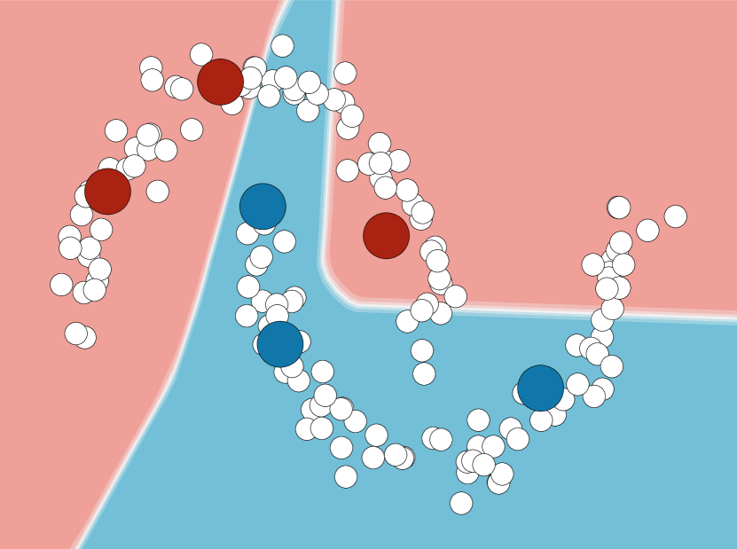
(a) no consistency loss

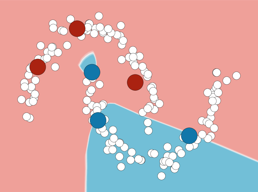
(b) one-way, clean student: $D(h_{\bm{\theta}}(\bm{x}),h_{\bm{\theta}^{\prime}}(T(\bm{x})))$

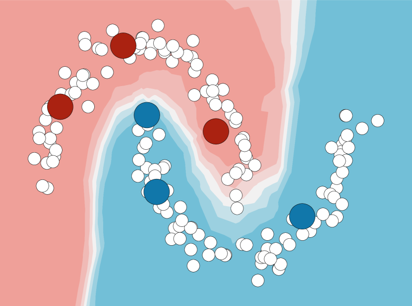
(c) one-way, clean teacher: $D(h_{\bm{\theta}^{\prime}}(\bm{x}),h_{\bm{\theta}}(T(\bm{x})))$

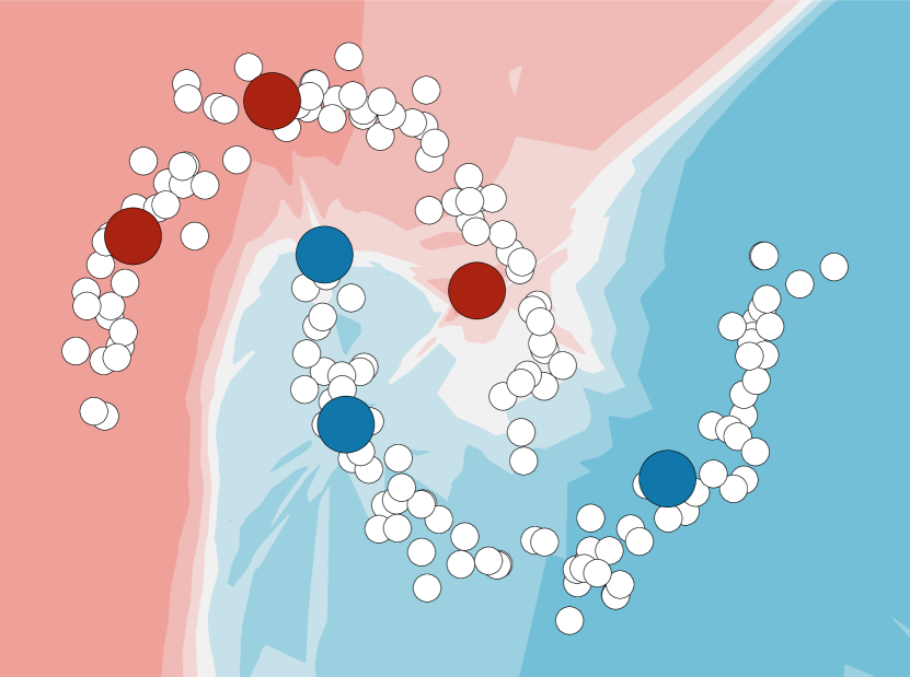
(d) two-way, one input clean: $D(h_{\bm{\theta}}(\bm{x}),h_{\bm{\theta}}(T(\bm{x})))$

Figure 1: A toy semi-supervised classification problem with 6 labeled (red, blue) and many unlabeled 2D datapoints (white). All setups involve 20 000 epochs of semi-supervised training with cross-entropy and default Adam optimization hyper-parameters. The consistency loss was set to none (1(a)), one-way with clean student (1(b)), one-way with clean teacher (1(c)), and two-way with one input clean (1(d)). One-way consistency with clean teacher outperforms all other formulations.

One-way consistency is especially advantageous in the dense prediction context since it does not require caching latent activations in the teacher. This allows for better training in many practical cases where model capacity is limited by GPU memory [52, 26]. In comparison with two-way consistency [29, 3], the proposed approach both improves generalization and approximately halves the training memory footprint.

This paper is an extended version of our preliminary conference report [19]. It exposes the elements of our method in much more detail and complements them with many new experiments. In particular, the most important additions are additional ablation and validation studies, full-resolution Cityscapes experiments, and a detailed analysis of a large-scale experiment that compares the contribution of coarse labels with semi-supervised learning on unlabeled images. The new experiments add more evidence in favor of one-way consistency with respect to other consistency variants, investigate the influence of particular components of our algorithm and various hyper-parameters, and investigate the behavior of the proposed algorithm in different data regimes (higher resolution, additional unlabeled images).

The consolidated paper proposes a simple and effective method for semi-supervised semantic segmentation. One-way consistency with clean teacher [38, 65, 14] outperforms the two-way formulation in our validation experiments. In addition, it retains the memory footprint of supervised training because the teacher activations depend on parameters that are treated as constants. Experiments with a standard convolutional architecture [6] reveal that our photometric and geometric perturbations lead to competitive generalization performance and outperform their counterpart from a recent related work [14]. A similar advantage can be observed in experiments with a recent efficient architecture [43], which offers a similar performance while requiring an order of magnitude less computation. To our knowledge, this is the first account of evaluation of semi-supervised algorithms for dense prediction with a model capable of real-time inference. This contributes to the goals of Green AI [55] by enabling competitive research with less environmental damage.

2 Related Work

Our work spans the fields of dense prediction and semi-supervised learning. The proposed methodology is most related to previous work in semi-supervised semantic segmentation.

2.1 Dense Prediction

Image-wide classification models usually achieve efficiency, spatial invariance, and integration of contextual information by gradual downsampling of representations and use of global spatial pooling operations. However, dense prediction also requires location accuracy. This emphasizes the trade-off between efficiency and quality of high-resolution features in model design. Some common designs use a classification backbone as a feature encoder and attach a decoder that restores the spatial resolution. Many approaches seek to enhance contextual information, starting with FCN-8s [32]. UNet [51] improves spatial details by directly using earlier representations of the encoder in a symmetric decoder. Further work improves efficiency with lighter decoders [26, 70]. Some models use context aggregation modules such as spatial pyramid pooling [71] and multi-scale inference [70, 44]. DeepLab [7] increases the receptive field through dilated convolutions and improves spatial details through CRF post-processing. HRNet [57] maintains the full resolution throughout the whole model and incrementally introduces parallel lower-resolution branches that exchange information between stages. Semantic segmentation gains much from ImageNet pre-trained encoders [7, 26].

2.2 Semi-Supervised Learning

Semi-supervised methods often rely on some of the following assumptions about the data distribution [4]: (1) similar inputs in high density regions correspond to similar outputs (smoothness assumption), (2) inputs form clusters separated by low-density regions and inputs within clusters are likely to correspond to similar outputs (cluster assumption), and (3) the data lies on a lower-dimensional manifold (manifold assumption). Semi-supervised methods devise various inductive biases that exploit such regularities for learning from unlabeled data.

Entropy minimization [17] encourages high confidence in unlabeled inputs. Such designs push decision boundaries towards low-density regions, under assumptions of clustered data and prediction smoothness. Pseudo-label training (or self-training) [68, 35, 24] also encourages high confidence (because of hard pseudo-labels) as well as consistency with a previously trained teacher. The basic forms of such algorithms do not achieve competitive performance on their own [42], but can be effective in conjunction with other approaches [66, 38]. Pseudo-labels can be made very effective by confidence-based selection and other processing [68, 35, 63]. Some concurrent work [63] uses the term pseudo-label as a synonym for processed teacher prediction in one-way consistency, but we do not follow this practice.

Many approaches exploit the smoothness assumption by enforcing prediction consistency across different versions of the same input or different model instances. Introducing knowledge about equivariance has been studied for understanding and learning useful image representations [16, 31] and improving dense prediction [64, 9, 47]. Exemplar training [12] associates patches with their original images (each image is a separate surrogate class). Temporal ensembling [29] enforces per-datapoint consistency between the current prediction and a moving average of past predictions. Mean Teacher [59] encourages consistency with a teacher whose parameters are an exponential moving average of the student’s parameters.

Clusterization of latent representations can be promoted by penalizing walks which start in a labeled example, pass over an unlabeled example, and end in another example with a different label [20]. PiCIE [9] obtains semantically meaningful segmentation without labels by jointly learning clustering and representation consistency under photometric and geometric perturbations.

MixMatch [1] encourages consistency between predictions in different MixUp perturbations of the same input. The average prediction is used as a pseudo-label for all variants of the input. Deep co-training [49] produces complementary models by encouraging them to be consistent while each is trained on adversarial examples of the other one.

Consistency losses may encourage trivial solutions, where all inputs give rise to the same output. This is not much of a problem in semi-supervised learning since there the trivial solution is inhibited through the supervised objective. Interestingly, recent work shows that a variant of simple one-way consistency evades trivial solutions even in the context of self-supervised representation learning [8, 60] .

Virtual adversarial training (VAT) [38] encourages one-way consistency between predictions in original datapoints and their adversarial perturbations. These perturbations are recovered by maximizing a quadratic approximation of the prediction divergence in a small $\mathrm{L}^{2}$ ball around the input. Better performance is often obtained by additionally encouraging low-entropy predictions [17]. Unsupervised data augmentation (UDA) [65] also uses a one-way consistency loss. FixMatch [27] shows that pseudo-label selection and processing can be useful in one-way consistency. However, instead of adversarial additive perturbations, they use random augmentations generated by RandAugment. Different from all previous approaches, we explore an exhaustive set of consistency formulations.

2.3 Semi-Supervised Semantic Segmentation

In the classic semi-supervised GAN (SGAN) setup, the classifier also acts as a discriminator which distinguishes between real data (both labeled and unlabeled) and fake data produced by the generator [54]. This approach has been adapted for dense prediction by expressing the discriminator as a segmentation network that produces dense C+1-way logits [56]. KE-GAN [48] additionally enforces semantic consistency of neighbouring predictions by leveraging label-similarity recovered from a large text corpus (MIT ConceptNet). A semantic segmentation model can also be trained as a GAN generator (AdvSemSeg) [23]. In this setup, the discriminator guesses whether its input is ground truth or generated by the segmentation network. The discriminator is also used to choose better predictions for use as pseudo-labels for semi-supervised training. s4GAN + MLMT [37] additionally post-processes the recovered dense predictions by emphasizing classes identified by an image-wide classifier trained with Mean Teacher [59]. The authors note that the image-wide classification component is not appropriate for datasets such as Cityscapes, where almost all images contain a large number of classes.

A recent approach enforces consistency between outputs of redundant decoders with noisy intermediate representations [45]. Other recent work studies pseudo-labeling in the dense prediction context [73, 5, 36]. Zhu et al. [73] observe advantages in hard pseudo-labels. A recent approach [3] proposes a two-way consistency loss, which is related to the $\Pi$-model [29], and perturbs both inputs with geometric warps. However, we show that perturbing only the student branch generalizes better and has a smaller training footprint. A concurrent work [28] successfully applies a contrastive loss [62, 21] between two branches which receive overlapping crops, and proposes a pixel-dependent consistency direction. Mean Teacher consistency with CutMix perturbations achieved state-of-the-art performance on half-resolution Cityscapes [14] prior to this work. Different than most presented approaches and similar to [73, 5, 14, 67], our method does not increase the training footprint [52]. In comparison with [73, 5, 67], our teacher is updated in each training step, which eliminates the need for multiple training episodes. In comparison with [14], this work proposes a perturbation model which results in better generalization and shows that simple one-way consistency can be competitive with Mean Teacher. None of the previous approaches addresses semi-supervised training of efficient dense prediction models. We examine the simplest forms of consistency, explain advantages of perturbing only the student with respect to other forms of consistency, and propose a novel perturbation model. None of the previous approaches considered semi-supervised training of efficient dense-prediction models, nor studied composite perturbations of photometry and geometry.

3 Method

We formulate dense consistency as a mean pixel-wise divergence between corresponding predictions in the clean image and its perturbed version. We perturb images with a composition of photometric and geometric transformations. Photometric transformations do not disturb the spatial layout of the input image. Geometric transformations affect the spatial layout of the input image, but the same kind of disturbance is expected at the model output. Ideally, our models should exhibit invariance to photometric transformations and equivariance to the geometric ones.

3.1 Notation

We typeset vectors and arrays in bold, sets in blackboard bold, and we underline random variables. $\operatorname{P}[{{\makebox[0.0pt]{}\mathclap{y}\text{\smash{\raisebox{0.39993pt}{$\mathclap{\underline{\hphantom{i}\vphantom{y}}}$}}}\makebox[0.0pt]{}}}|{{\makebox[0.0pt]{}\mathclap{\bm{x}}\text{\smash{\raisebox{0.39993pt}{$\mathclap{\underline{\hphantom{i}\vphantom{\bm{x}}}}$}}}\makebox[0.0pt]{}}}=\bm{x}]$ denotes the distribution of a random variable ${{\makebox[0.0pt]{}\mathclap{y}\text{\smash{\raisebox{0.39993pt}{$\mathclap{\underline{\hphantom{i}\vphantom{y}}}$}}}\makebox[0.0pt]{}}}|\bm{x}$, while $\operatorname{P}(y|\bm{x})$ is a shorthand for the probability $\operatorname{P}({{\makebox[0.0pt]{}\mathclap{y}\text{\smash{\raisebox{0.39993pt}{$\mathclap{\underline{\hphantom{i}\vphantom{y}}}$}}}\makebox[0.0pt]{}}}=y|{{\makebox[0.0pt]{}\mathclap{\bm{x}}\text{\smash{\raisebox{0.39993pt}{$\mathclap{\underline{\hphantom{i}\vphantom{\bm{x}}}}$}}}\makebox[0.0pt]{}}}=\bm{x})$. We denote the expectation of a function of a random variable as e.g. $\operatorname*{\mathrm{I\kern-2.81998ptE}}_{{{\makebox[0.0pt]{}\mathclap{\bm{\tau}}\text{\smash{\raisebox{0.27995pt}{$\mathclap{\underline{\hphantom{i}\vphantom{\bm{\tau}}}}$}}}\makebox[0.0pt]{}}}}f(\bm{\tau})$. We use similar notation to denote the average over a set: $\operatorname*{\mathrm{I\kern-2.81998ptE}}_{\bm{x}\in\mathbbmsl{D}}f(\bm{x})$. We denote cross-entropy with $\mathrm{H}_{{{\makebox[0.0pt]{}\mathclap{y}\text{\smash{\raisebox{0.27995pt}{$\mathclap{\underline{\hphantom{i}\vphantom{y}}}$}}}\makebox[0.0pt]{}}}}({{\makebox[0.0pt]{}\mathclap{y}\text{\smash{\raisebox{0.39993pt}{$\mathclap{\underline{\hphantom{i}\vphantom{y}}}$}}}\makebox[0.0pt]{}}}^{*})\coloneqq\operatorname*{\mathrm{I\kern-2.81998ptE}}_{y\sim{{\makebox[0.0pt]{}\mathclap{\bm{y}}\text{\smash{\raisebox{0.27995pt}{$\mathclap{\underline{\hphantom{i}\vphantom{\bm{y}}}}$}}}\makebox[0.0pt]{}}}^{*}}\ln\operatorname{\mathrm{p}}({{\makebox[0.0pt]{}\mathclap{y}\text{\smash{\raisebox{0.39993pt}{$\mathclap{\underline{\hphantom{i}\vphantom{y}}}$}}}\makebox[0.0pt]{}}}=y)$, and entropy with $\mathrm{H}({{\makebox[0.0pt]{}\mathclap{y}\text{\smash{\raisebox{0.39993pt}{$\mathclap{\underline{\hphantom{i}\vphantom{y}}}$}}}\makebox[0.0pt]{}}})$ [41]. We use Python-like array indexing notation.

We denote the labeled dataset as $\mathbbmsl{D}_{\text{l}}$, and the unlabeled dataset as $\mathbbmsl{D}_{\text{u}}$. We consider input images $\bm{x}\in[0,1]^{H\times W\times 3}$ and dense labels $\bm{y}\in\{1\mkern 1.5mu{..}\mkern 1.5muC\}^{H\times W}$. A model instance maps an image to per-pixel class probabilities: $h_{\bm{\theta}}(\bm{x})_{[i,j,c]}=\operatorname{P}({{\makebox[0.0pt]{}\mathclap{\bm{y}}\text{\smash{\raisebox{0.39993pt}{$\mathclap{\underline{\hphantom{i}\vphantom{\bm{y}}}}$}}}\makebox[0.0pt]{}}}_{[i,j]}=c|\bm{x},\bm{\theta})$. For convenience, we identify output vectors of class probabilities with distributions: $h_{\bm{\theta}}(\bm{x})_{[i,j]}\equiv\operatorname{P}[{{\makebox[0.0pt]{}\mathclap{\bm{y}}\text{\smash{\raisebox{0.39993pt}{$\mathclap{\underline{\hphantom{i}\vphantom{\bm{y}}}}$}}}\makebox[0.0pt]{}}}_{[i,j]}|\bm{x},\bm{\theta}]$.

3.2 Dense One-Way Consistency

We adapt one-way consistency [38, 65] for dense prediction under our perturbation model $T_{\bm{\tau}}=T^{\text{G}}_{\bm{\gamma}}\circ T^{\text{P}}_{\bm{\varphi}}$, where $T^{\text{G}}_{\bm{\gamma}}$ is a geometric warp, $T^{\text{P}}_{\bm{\varphi}}$ a per-pixel photometric perturbation, and $\bm{\tau}=(\bm{\gamma},\bm{\varphi})$ perturbation parameters. $T^{\text{G}}_{\bm{\gamma}}$ displaces pixels with respect to a dense deformation field. The same geometric warp is applied to the student input and the teacher output. Figure 2 illustrates the computational graph of the resulting dense consistency loss. In simple one-way consistency, the teacher parameters $\bm{\theta}^{\prime}$ are a frozen copy of the student parameter $\bm{\theta}$. In Mean Teacher, $\bm{\theta}^{\prime}$ is a moving average of $\bm{\theta}$. In simple two-way consistency, both branches use the same $\bm{\theta}$ and are subject to gradient propagation.

Figure 2: Dense one-way consistency with clean teacher. Top branch: the input is fed to the teacher $h_{\bm{\theta}^{\prime}}$. The resulting predictions are perturbed with geometric perturbations $T^{\text{G}}_{\bm{\gamma}}$. Bottom branch: the input is perturbed with geometric and photometric perturbations and fed to the student $h_{\bm{\theta}}$. The loss $D$ corresponds to the average pixel-wise KL divergence between the two branches. Gradients are computed only in the blue part of the graph.

A general semi-supervised training criterion $L(\bm{\theta};\mathbbmsl{D}_{\text{l}},\mathbbmsl{D}_{\text{u}})$ can be expressed as a weighted sum of a supervised term $L_{\text{s}}$ over labeled data and an unsupervised consistency term $L_{\text{c}}$:

$$L(\bm{\theta};\mathbbmsl{D}_{\text{l}},\mathbbmsl{D}_{\text{u}})=\operatorname*{\mathrm{I\kern-2.81998ptE}}_{(\bm{x},\bm{y})\in\mathbbmsl{D}_{\text{l}}}L_{\text{s}}(\bm{\theta};\bm{x},\bm{y})+\alpha\operatorname*{\mathrm{I\kern-2.81998ptE}}_{\bm{x}\in\mathbbmsl{D}_{\text{u}}}\operatorname*{\mathrm{I\kern-2.81998ptE}}_{{{\makebox[0.0pt]{}\mathclap{\bm{\tau}}\text{\smash{\raisebox{0.27995pt}{$\mathclap{\underline{\hphantom{i}\vphantom{\bm{\tau}}}}$}}}\makebox[0.0pt]{}}}}L_{\text{c}}(\bm{\theta};\bm{x},\bm{\tau})\;.$$ (2)

In our experiments, $L_{\text{s}}$ is the usual mean per-pixel cross entropy with $\mathrm{L}^{2}$ regularization. We stochastically estimate the expectation over perturbation parameters ${{\makebox[0.0pt]{}\mathclap{\bm{\tau}}\text{\smash{\raisebox{0.39993pt}{$\mathclap{\underline{\hphantom{i}\vphantom{\bm{\tau}}}}$}}}\makebox[0.0pt]{}}}$ with one sample per training step.

We formulate the unsupervised term $L_{\text{c}}$ at pixel $(i,j)$ as a one-way divergence $D$ between the prediction in the perturbed image and its interpolated correspondence in the clean image. The proposed loss encourages the trained model to be equivariant to $T^{\text{G}}_{\bm{\gamma}}$ and invariant to $T^{\text{P}}_{\bm{\varphi}}$:

$$L_{\text{c}}^{i,j}(\bm{\theta};\bm{x},\bm{\tau})=D(T^{\text{G}}_{\bm{\gamma}}(h_{\bm{\theta}^{\prime}}(\bm{x}))_{[i,j]},h_{\bm{\theta}}((T^{\text{G}}_{\bm{\gamma}}\circ T^{\text{P}}_{\bm{\varphi}})(\bm{x}))_{[i,j]})\;.$$ (3)

We use a validity mask $\bm{v}^{\bm{\gamma}}\in\{0,1\}^{H\times W}$, $\bm{v}^{\bm{\gamma}}_{[i,j]}={\mathinner{\left\llbracket{T^{\text{G}}_{\bm{\gamma}}(\mathbf{1}_{H\times W})_{[i,j]}=1}\right\rrbracket}}$ to ensure that the loss is unaffected by padding sampled from outside of $[1,H]\times[1,W]$. A vector produced by $T^{\text{G}}_{\bm{\gamma}}(h_{\bm{\theta}}(\bm{x}))_{[i,j]}$ represents a valid distribution wherever $\bm{v}^{\bm{\gamma}}_{[i,j]}=1$. Finally, we express the consistency term $L_{\text{c}}$ as a mean contribution over all pixels:

$$L_{\text{c}}(\bm{\theta};\bm{x},\bm{\tau})=\frac{1}{\sum(\bm{v}^{\bm{\gamma}})}\sum_{i,j}\bm{v}^{\bm{\gamma}}_{[i,j]}L_{\text{c}}^{i,j}(\bm{\theta};\bm{x},\bm{\tau})\;.$$ (4)

Recall that the gradient is not computed with respect to $\bm{\theta}^{\prime}$. Consequently, $L_{\text{c}}$ allows gradient propagation only towards the perturbed image. We refer to such training as one-way consistency with clean teacher (and perturbed student). Such formulation provides two distinct advantages over other kinds of consistency. First, predictions in perturbed images are pulled towards predictions in clean images. This improves generalization when the perturbations are stronger than data augmentations used in $L_{\text{s}}$ (cf. Figures 3 and 1). Second, we do not have to cache teacher activations during training since the gradients propagate only towards the student branch. Hence, the proposed semi-supervised objective does not constrain model complexity with respect to the supervised baseline.

We use KL divergence as a principled choice for $\mathit{D}$:

$$\mathit{D}({{\makebox[0.0pt]{}\mathclap{y}\text{\smash{\raisebox{0.39993pt}{$\mathclap{\underline{\hphantom{i}\vphantom{y}}}$}}}\makebox[0.0pt]{}}},\vphantom{{{\makebox[0.0pt]{}\mathclap{y}\text{\smash{\raisebox{0.39993pt}{$\mathclap{\underline{\hphantom{i}\vphantom{y}}}$}}}\makebox[0.0pt]{}}}}\smash[t]{\tilde{{{\makebox[0.0pt]{}\mathclap{y}\text{\smash{\raisebox{0.39993pt}{$\mathclap{\underline{\hphantom{i}\vphantom{y}}}$}}}\makebox[0.0pt]{}}}}})\coloneqq\operatorname*{\mathrm{I\kern-2.81998ptE}}_{{{\makebox[0.0pt]{}\mathclap{y}\text{\smash{\raisebox{0.27995pt}{$\mathclap{\underline{\hphantom{i}\vphantom{y}}}$}}}\makebox[0.0pt]{}}}}\ln\frac{\operatorname{P}({{\makebox[0.0pt]{}\mathclap{y}\text{\smash{\raisebox{0.39993pt}{$\mathclap{\underline{\hphantom{i}\vphantom{y}}}$}}}\makebox[0.0pt]{}}}=y)}{\operatorname{P}(\vphantom{{{\makebox[0.0pt]{}\mathclap{y}\text{\smash{\raisebox{0.39993pt}{$\mathclap{\underline{\hphantom{i}\vphantom{y}}}$}}}\makebox[0.0pt]{}}}}\smash[t]{\tilde{{{\makebox[0.0pt]{}\mathclap{y}\text{\smash{\raisebox{0.39993pt}{$\mathclap{\underline{\hphantom{i}\vphantom{y}}}$}}}\makebox[0.0pt]{}}}}}=y)}=\mathrm{H}_{\vphantom{{{\makebox[0.0pt]{}\mathclap{y}\text{\smash{\raisebox{0.27995pt}{$\mathclap{\underline{\hphantom{i}\vphantom{y}}}$}}}\makebox[0.0pt]{}}}}\smash[t]{\tilde{{{\makebox[0.0pt]{}\mathclap{y}\text{\smash{\raisebox{0.27995pt}{$\mathclap{\underline{\hphantom{i}\vphantom{y}}}$}}}\makebox[0.0pt]{}}}}}}({{\makebox[0.0pt]{}\mathclap{y}\text{\smash{\raisebox{0.39993pt}{$\mathclap{\underline{\hphantom{i}\vphantom{y}}}$}}}\makebox[0.0pt]{}}})-\mathrm{H}({{\makebox[0.0pt]{}\mathclap{y}\text{\smash{\raisebox{0.39993pt}{$\mathclap{\underline{\hphantom{i}\vphantom{y}}}$}}}\makebox[0.0pt]{}}})\;.$$ (5)

Note that the entropy term $-\mathrm{H}({{\makebox[0.0pt]{}\mathclap{y}\text{\smash{\raisebox{0.39993pt}{$\mathclap{\underline{\hphantom{i}\vphantom{y}}}$}}}\makebox[0.0pt]{}}})$ does not affect parameter updates since the gradients are not propagated through $\bm{\theta}^{\prime}$. Hence, one-way consistency does not encourage increasing entropy of model predictions in clean images. Several researchers have observed improvement after adding an entropy minimization term [17] to the consistency loss [38, 65]. This practice did not prove beneficial in our initial experiments.

Note that two-way consistency [29, 3] would be obtained by replacing $\bm{\theta}^{\prime}$ with $\bm{\theta}$. It would require caching latent activations for both model instances, which approximately doubles the training footprint with respect to the supervised baseline. This would be undesirable due to constraining the feasible capacity of the deployed models [52, 22].

We argue that consistency with clean teacher generalizes better than consistency with clean student since strong perturbations may push inputs beyond the natural manifold and spoil predictions (cf. Figure 1). Moreover, perturbing both branches sometimes results in learning to map all perturbed pixels to similar arbitrary predictions (e.g. always the same class) [18]. Figure 3 illustrates that consistency training has the best chance to succeed if the teacher is applied to the clean image, and the student learns on the perturbed image.

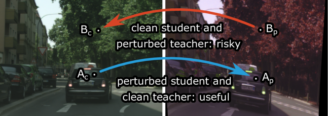
Figure 3: Two variants of one-way consistency training on a clean image (left) and its perturbed version (right). The arrows designate information flow from the teacher to the student. The proposed clean-teacher formulation trains in the perturbed pixels ($\mathrm{A_{p}}$) according to the corresponding predictions in the clean image ($\mathrm{A_{c}}$). The reverse formulation (training in $\mathrm{B_{c}}$ according to the prediction in $\mathrm{B_{p}}$) worsens performance since strongly perturbed images often give rise to less accurate predictions.

3.3 Photometric Component of the Proposed Perturbation Model

We express pixel-level photometric transformations as a composition of five simple perturbations with five image-wide parameters $\bm{\varphi}=(b,s,h,c,\bm{\pi})$. These perturbations are applied in each pixel in the following order: (1) brightness is shifted by adding $b$ to all channels, (2) saturation is multiplied with $s$, (3) hue is shifted by addition with $h$, (4) contrast is modulated by multiplying all channels with $c$, and (5) RGB channels are randomly permuted according to $\bm{\pi}$. The resulting compound transformation $T^{\text{P}}_{\bm{\varphi}}$ is independently applied to all image pixels.

Our training procedure randomly picks image-wide parameters $\bm{\varphi}$ for each unlabeled image. The parameters are sampled as follows: $b\sim\mathcal{U}(-0.25,0.25)$, $s\sim\mathcal{U}(0.25,2)$, $h\sim\mathcal{U}(-36^{\circ},36^{\circ})$, $c\sim\mathcal{U}(0.25,2)$, and $\bm{\pi}\sim\mathcal{U}(\mathbb{S}_{3})$, where $\mathbb{S}_{3}$ represents the set of all $6$ 3-element permutations.

3.4 Geometric Component of the Proposed Perturbation Model

We formulate a fairly general class of parametric geometric transformations by leveraging thin plate splines (TPS) [13, 2]. We consider the 2D TPS warp $f\colon\mathbb{R}^{2}\to\mathbb{R}^{2}$ which maps each image coordinate pair $\bm{q}$ to the relative 2D displacement of its correspondence $\bm{q}^{\prime}$: $f(\bm{q})=\bm{q}^{\prime}-\bm{q}$. TPS warps minimize the bending energy (curvature) $\int_{\operatorname{dom}(f)}\|\frac{\partial^{2}f(\bm{q})}{\partial\bm{q}^{2}}\|_{\text{F}}^{2}\operatorname{d\!}\bm{q}$ given a set of control points and their displacements $\{(\bm{c}_{i},\bm{d}_{i})\colon i=1\mkern 1.5mu{..}\mkern 1.5mun\}\subset\mathbb{R}^{2}\times\mathbb{R}^{2}$. In simple words, a TPS warp produces a smooth deformation field which optimally satisfies all constraints $f(\bm{c}_{i})=\bm{d}_{i}$. In the 2D case, the solution of the TPS problem takes the following form:

$$f(\bm{q})=\bm{A}\begin{bmatrix}1\\ \bm{q}\end{bmatrix}+\bm{W}\begin{bmatrix}\phi(\|\bm{q}-\bm{c}_{i}\|)\end{bmatrix}_{i=1\mkern 1.5mu{..}\mkern 1.5mun}^{\mathsf{T}}\;.$$ (6)

In the above equation, $\bm{q}$ denotes a 2D coordinate vector to be transformed, $\bm{A}$ is a $2\times 3$ affine transformation matrix, $\bm{W}$ is a $2\times n$ control point coefficient matrix, and $\phi(r)=r^{2}\ln(r)$. Such a 2D TPS warp is equivariant to rotation and translation [2]. That is, $f(T(\bm{q}))=T(f(\bm{q}))$ for every composition of rotation and translation $T$.

TPS parameters $\bm{A}$ and $\bm{W}$ can be determined as a solution of a standard linear system which enforces deformation constraints $(\bm{c}_{i},\bm{d}_{i})$, and square-integrability of second derivatives of $f$. When we determine $\bm{A}$ and $\bm{W}$, we can easily transform entire images.

We first consider images as continuous domain functions and later return to images as arrays from $[0,1]^{H\times W\times 3}$. Let $I\colon\operatorname{dom}(I)\to\mathinner{[0,1]}^{3}$ be the original image of size $(W,H)$, where $\operatorname{dom}(I)=\mathinner{[0,W]}\times\mathinner{[0,H]}$. Then the transformed image $I^{\prime}$ can be expressed as

$$I^{\prime}(\bm{q}+f(\bm{q}))=\begin{cases}I(\bm{q}),&\bm{q}\in\operatorname{dom}(I),\\ \mathbf{0},&\text{otherwise.}\end{cases}$$ (7)

The resulting formulation is known as forward warping [58] and is tricky to implement. We, therefore, prefer to recover the reverse transformation $\vphantom{f}\smash[t]{\tilde{f}}$, which can be done by replacing each control point $\bm{c}_{i}$ with $\bm{c}_{i}^{\prime}=\bm{c}_{i}+\bm{d}_{i}$. Then the transformed image is:

$$\vphantom{I}\smash[t]{\tilde{I}}(\bm{q}^{\prime})=\begin{cases}I(\bm{q}^{\prime}-\vphantom{f}\smash[t]{\tilde{f}}(\bm{q}^{\prime})),&\bm{q}^{\prime}-\vphantom{f}\smash[t]{\tilde{f}}(\bm{q}^{\prime})\in\operatorname{dom}(I),\\ \mathbf{0},&\text{otherwise.}\end{cases}$$ (8)

This formulation is known as backward warping [58]. It can be easily implemented for discrete images by leveraging bilinear interpolation. Contemporary frameworks already include the implementations for GPU hardware. Hence, the main difficulty is to determine the TPS parameters by solving two linear systems with $(n+3)\times(n+3)$ variables [2].

In our experiments, we use $n=4$ control points corresponding to the centers of the four image quadrants: $(\bm{c}_{1}^{\prime},..,\bm{c}_{4}^{\prime})=([\frac{1}{4}H,\frac{1}{4}W]^{\mathsf{T}},..,[\frac{3}{4}H,\frac{3}{4}W]^{\mathsf{T}})$. The parameters of our geometric transformation are four 2D displacements $\bm{\gamma}=(\bm{d}_{1},..,\bm{d}_{4})$. Let $f_{\bm{\gamma}}$ denote the resulting TPS warp. Then we can express our transformation as $T^{\text{G}}_{\bm{\gamma}}(\bm{x})=\mathrm{backward\_warp}(\bm{x},f_{\bm{\gamma}})$.

Our training procedure picks a random $\bm{\gamma}$ for each unlabeled image. Each displacement is sampled from a 2D normal distribution $\mathcal{N}(\mathbf{0}_{2},0.05H\cdot\mathbf{I}_{2})$, where $H$ is the training crop height.

3.5 Training Procedure

Algorithm LABEL:alg:training sketches a procedure for recovering gradients of the proposed semi-supervised loss (2) on a mixed batch of labeled and unlabeled examples. For simplicity, we make the following changes in notation here: $\bm{x}_{\text{l}}$ and $\bm{y}_{\text{l}}$ are batches of size $B_{\text{l}}$, $\bm{x}_{\text{u}}$, $\bm{\gamma}$ and $\bm{\varphi}$ batches of size $B_{\text{u}}$, and all functions are applied to batches. The algorithm computes the gradient of the supervised loss, discards cached activations, computes the teacher predictions, applies the consistency loss (3), and finally accumulates the gradient contributions of the two losses. Backpropagation through one-way consistency with clean teacher requires roughly as much caching as the supervised baseline. Hence, our approach constrains the model complexity much less than the two-way consistency.

⬇

# $\vec x_\text{u}$, $\vec\gamma$, $\vec\varphi$, $\vec p_\text{t}$, $\vec p_\text{s}$, and $\vec v$ contain batches of $B_\text{u}$ elements.

# $\vec x_\text{l}$, $\vec y$, and $\vec p_\text{l}$ contain batches of $B_\text{l}$ elements.

procedure compute_loss_gradient($h, \vec\theta, \vec x_\text{l}, \vec y_\text{l}, \vec x_\text{u}, \vec\gamma, \vec\varphi$):

$\vec\theta’ \gets \mathrm{frozen\_copy}(\vec\theta)$ # simple one-way

# supervised loss

$\vec p_\text{l} \gets h_{\vec\theta}(\vec x_\text{l})$

$L_\text{s} \gets \mathrm{CE}(\vec y_\text{l}, \vec p_\text{l})$

$\vec g \gets \nabla_{\vec\theta}L_\text{s}$ # clears cached activations

# unsupervised loss

with no_grad(): # activations not cached here

$\vec p_\text{t} \gets T^\text{G}_{\vec\gamma}(h_{\vec\theta’}(\vec x_\text{u}))$ # clean teacher

$\vec p_\text{s} \gets h_{\vec\theta}((T^\text{G}_{\vec\gamma} \circ T^\text{P}_{\vec\varphi})(\vec x_\text{u}))$ # perturbed student

$\vec v \gets \lfloor T^\text{G}_{\vec\gamma}(\cvec 1_{B_\text{u}\times H\times W}) \rfloor$ # validity mask

$L_\text{c} \gets \alpha\cdot \mathrm{KL\_masked}(\vec p_\text{t}, \vec p_\text{s}, \vec v)$

$\vec g \gets \vec g + \nabla_{\vec\theta}L_\text{c}$

return $\vec g$

Figure 4 illustrates GPU memory allocation during a semi-supervised training iteration of a SwiftNet-RN34 model with one-way and two-way consistency. We recovered these measurements by leveraging the following functions of the torch.cuda package: max_memory_allocated, memory_allocated, reset_peak_memory_stats, and empty_cache. The training was carried out on a RTX A4500 GPU. Numbers on the x-axis correspond to lines of the pseudo-code in Algorithm LABEL:alg:training. Line 9 backpropagates through the supervised loss and caches the gradients. The memory footprint briefly peaks due to temporary storage and immediately declines since PyTorch automatically releases all cached activations immediately after the backpropagation. Line 13 computes the teacher output. This step does not cache intermediate activations since we freeze parameters with torch.no_grad. Line 16 computes the unsupervised loss, which requires caching of activations on a large spatial resolution. The memory footprint briefly peaks since we delete perturbed inputs and teacher predictions immediately after line 16 (for simplicity, we omit opportunistic deletions from Algorithm 1). Line 17 triggers the backpropagation algorithm and accumulates the gradients of the consistency loss. The memory footprint briefly peaks due to temporary storage and immediately declines due to automatic deletion of cached activations. At this point, the memory footprint is slightly greater than at line 4 since we still hold the supervised predictions in order to accumulate recognition performance on the training dataset.

The ratio between memory allocations at lines 16 and 9 reveals the relative memory overhead of our semi-supervised approach. Note that the absolute overhead is model independent since it corresponds to the total size of perturbed inputs and predictions, and intermediate results of dense KL-divergence. On the other hand, the memory footprint of the supervised baseline is model dependent since it reflects computational complexity of the backbone. Consequently, the relative overhead approaches 1 as the model size increases, and is around 1.26 for SwiftNet-RN34.

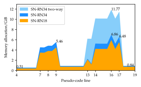
Figure 4: Total GPU memory allocation during and after execution of particular lines from Algorithm LABEL:alg:training during the 2nd iteration of training. Our PyTorch implementations involve SwiftNet-RN18 and SwiftNet-RN34 models with one-way and two-way consistency, $768\times 768$ crops, and batch sizes $(B_{\text{l}},B_{\text{u}})=(8,8)$. Line 9 computes the supervised gradient. Line 13 computes the teacher output (without caching interemediate activations). Lines 16 and 17 compute the consistency loss and its gradient.

4 Results

Our experiments evaluate one-way consistency with clean teacher and a composition of photometric and geometric perturbations ($T_{\gamma}^{G}\circ T_{\phi}^{P}$). We compare our approach with other kinds of consistency and the state of the art in semi-supervised semantic segmentation. We denote simple one-way consistency as ”simple”, Mean Teacher [59] as ”MT”, and our perturbations as ”PhTPS”. In experiments that compare consistency variants, ”1w” denotes one-way, ”2w” denotes two way, ”ct” denotes clean teacher, ”cs” denotes clean student, and ”2p” denotes both inputs perturbed. We present semi-supervised experiments in several semantic segmentation setups as well as in image-classification setups on CIFAR-10. Our implementations are based on the PyTorch framework [46].

4.1 Experimental Setup

Datasets. We perform semantic segmentation on Cityscapes [10], and image classification on CIFAR-10. Cityscapes contains 2975 training, 500 validation and 1525 testing images with resolution $1024\times 2048$. Images are acquired from a moving vehicle during daytime and fine weather conditions. We present half-resolution and full-resolution experiments. We use bilinear interpolation for images and nearest neighbour subsampling for labels. Some experiments on Cityscapes also use the coarsely labeled Cityscapes subset (”train-extra”) that contains 19998 images. CIFAR-10 consists of 50000 training and 10000 test images of resolution $32\times 32$.

Common setup. We include both unlabeled and labeled images in $\mathbbmsl{D}_{\text{u}}$, which we use for the consistency loss. We train on batches of $B_{\text{l}}$ labeled and $B_{\text{u}}$ unlabeled images. We perform $\left\lfloor|\mathbbmsl{D}_{\text{l}}|/B_{\text{l}}\right\rfloor$ training steps per epoch. We use the same perturbation model across all datasets and tasks (TPS displacements are proportional to image size), which is likely suboptimal [11]. Batch normalization statistics are updated only in non-teacher model instances with clean inputs except for full-resolution Cityscapes, for which updating the statistics in the perturbed student performed better in our validation experiments (cf. Appendix B). The teacher always uses the estimated population statistics, and does not update them. In Mean Teacher, the teacher uses an exponential moving average of the student’s estimated population statistics.

Semantic segmentation setup. Cityscapes experiments involve the following models: SwiftNet with ResNet-18 (SwiftNet-RN18) or ResNet-34 (SwiftNet-RN34), and DeepLab v2 with a ResNet-101 backbone. We initialize the backbones with ImageNet pre-trained parameters. We apply random scaling, cropping, and horizontal flipping to all inputs and segmentation labels. We refer to such examples as clean. We schedule the learning rate according to $e\mapsto\eta\cos(e\pi/2)$, where $e\in[0..1]$ is the fraction of epochs completed. This alleviates the generalization drop at the end of training with standard cosine annealing [33]. We use learning rates $\eta=4\cdot 10^{-4}$ for randomly initialized parameters and $\eta=10^{-4}$ for pre-trained parameters. We use Adam with $(\beta_{1},\beta_{2})=(0.9,0.99)$. The L² regularization weight in supervised experiments is $10^{-4}$ for randomly initialized and $2.5\cdot 10^{-5}$ for pre-trained parameters [43]. We have found that such L² regularization is too strong for our full-resolution semi-supervised experiments. Thus, we use a 4$\times$ smaller weight there. Based on early validation experiments, we use $\alpha=0.5$ unless stated otherwise. Batch sizes are $(B_{\text{l}},B_{\text{u}})=(8,8)$ for SwiftNet-RN18 [43] and $(B_{\text{l}},B_{\text{u}})=(4,4)$ for DeepLab v2 (ResNet-101 backbone) [6]. The batch size in corresponding supervised experiments is $B_{\text{l}}$.

In half-resolution Cityscapes experiments the size of crops is $448\times 448$ and the logarithm of the scaling factor is sampled from $\mathcal{U}(\ln(1.5^{-1}),\ln(1.5))$. We train SwiftNet for $200\cdot\frac{2975}{|\mathbbmsl{D}_{\text{l}}|}$ epochs ($200$ epochs or $74200$ iterations when all labels are used), and DeepLab v2 for $100\cdot\frac{2975}{|\mathbbmsl{D}_{\text{l}}|}$ epochs ($100$ epochs or $74300$ iterations when all labels are used). In comparison with SwiftNet-RN18, DeepLab v2 incurs a 12-fold per-image slowdown during supervised training. However, it also requires less epochs since it has very few parameters with random initialization. Hence, semi-supervised DeepLab v2 trains more than 4$\times$ slower than SwiftNet-RN18 on RTX 2080Ti. Appendix A.2 presents more detailed comparisons of memory and time requirements of different semi-supervised algorithms.

Our full-resolution experiments only use SwiftNet models. The crop size is $768\times 768$ and the spatial scaling is sampled from $\mathcal{U}(2^{-1},2)$. The number of epochs is 250 when all labels are used. The batch size is $8$ in supervised experiments, and $(B_{\text{l}},B_{\text{u}})=(8,8)$ in semi-supervised experiments.

Appendix A.1 presents an overview and comparison of hyper-parameters with other consistency-based methods that are compared in the experiments.

Classification setup. Classification experiments target CIFAR-10 and involve the Wide ResNet model WRN-28-2 with standard hyper-parameters [69]. We augment all training images with random flips, padding and random cropping. We use all training images (including labeled images) in $\mathbbmsl{D}_{\text{u}}$ for the consistency loss. Batch sizes are $(B_{\text{l}},B_{\text{u}})=(128,640)$. Thus, the number of iterations per epoch is $\left\lfloor\frac{|\mathbbmsl{D}_{\text{l}}|}{128}\right\rfloor$. For example, only one iteration is performed if $|\mathbbmsl{D}_{\text{l}}|=250$. We run $1000\cdot\frac{4000}{|\mathbbmsl{D}_{\text{l}}|}$ epochs in semi-supervised, and $100$ epochs in supervised training. We use default VAT hyper-parameters $\xi=10^{-6}$, $\epsilon=10$, $\alpha=1$ [38]. We perform photometric perturbations as described, and sample TPS displacements from $\mathcal{N}(\mathbf{0},3.2\cdot\mathbf{I}_{2})$.

Evaluation. We report generalization performance at the end of training. We report sample means and sample standard deviations (with Bessel’s correction) of the corresponding evaluation metric ($\mathrm{mIoU}$ or classification accuracy) of $5$ training runs, evaluated on the corresponding validation dataset.

4.2 Semantic Segmentation on Half-Resolution Cityscapes

Table 1 compares our approach with the previous state of the art. We train using different proportions of training labels and evaluate mIoU on half-resolution Cityscapes val. The top section presents the previous work [37, 23, 36, 14]. The middle section presents our experiments based on DeepLab v2 [6]. Note that here we outperform some previous work due to more involved training (as described in Section 4.1). since that would be a method of choice in all practical applications. Hence, we get consistently greater performance. We perform a proper comparison with [14] by using our training setup in combination with their method. Our MT-PhTPS outperforms MT-CutMix with L2 loss and confidence thresholding when 1/4 or more labels are available, while underperforming with 1/8 labels.

The bottom section involves the efficient model SwiftNet-RN18. Our perturbation model outperforms CutMix both with simple consistency, as well as with Mean Teacher. Overall, Mean Teacher outperforms simple consistency. We observe that DeepLab v2 and SwiftNet-RN18 get very similar benefits from the consistency loss. SwiftNet-RN18 comes out as a method of choice due to about 12$\times$ faster inference than DeepLab v2 with ResNet-101 on RTX 2080Ti (see Appendix A.2 for more details). Experiments from the middle and the bottom section use the same splits to ensure a fair comparison.

Table 1: Semantic segmentation performance (mIoU/%) on half-resolution Cityscapes val after training with different proportions of labeled data. The top section reviews experiments from previous work. The middle section presents our experiments with DeepLab v2. The bottom section presents our experiments with SwiftNet-RN18. We run experiments across 5 different dataset splits and report mean mIoUs with standard deviations. The subscript ”$\sim$[14]” denotes training with $\mathrm{L^{2}}$ loss, confidence thresholding, and $\alpha=1$, as proposed in [14]. Best results overall are bold, and best results within sections are underlined.

Method	Label proportion
	$1/8$	$1/4$	$1/2$	$1/1$
DLv2-RN101 supervised [37, 14]	$56.2_{\phantom{0.0}}$	$60.2_{\phantom{0.0}}$	$64.6^{1}_{\phantom{0.0}}$	$66.0_{\phantom{0.0}}$
DLv2-RN101 s4GAN+MLMT [37]	$59.3_{\phantom{0.0}}$	$61.9_{\phantom{0.0}}$	–	$65.8_{\phantom{0.0}}$
DLv2-RN101 supervised [23]	$55.5_{\phantom{0.0}}$	$59.9_{\phantom{0.0}}$	$64.1_{\phantom{0.0}}$	$66.4_{\phantom{0.0}}$
DLv2-RN101 AdvSemSeg [23]	$58.8_{\phantom{0.0}}$	$62.3_{\phantom{0.0}}$	$65.7_{\phantom{0.0}}$	$67.7_{\phantom{0.0}}$
DLv2-RN101 supervised [36]	$56.0_{\phantom{0.0}}$	$60.5_{\phantom{0.0}}$	–	$66.0_{\phantom{0.0}}$
DLv2-RN101 ECS [36]	$\underline{60.3}_{\phantom{0.0}}$	$\underline{63.8}_{\phantom{0.0}}$	–	$\underline{67.7}_{\phantom{0.0}}$
DLv2-RN101 MT-CutMix [14]	$\underline{60.3}_{1.2}$	$\underline{63.9}_{0.7}$	–	$\underline{67.7}_{0.4}$
DLv2-RN101 supervised	$56.4_{0.4}$	$61.9_{1.1}$	$66.6_{0.6}$	$69.8_{0.4}$
DLv2-RN101 MT-CutMix$\sim$[14]	$\mathbf{63.2}_{1.4}$	$65.6_{0.8}$	$67.6_{0.4}$	$70.0_{0.3}$
DLv2-RN101 MT-PhTPS	$61.5_{1.0}$	$\mathbf{66.4}_{1.1}$	$\mathbf{69.0}_{0.6}$	$\mathbf{71.0}_{0.7}$
SN-RN18 supervised	$55.5_{0.9}$	$61.5_{0.5}$	$66.9_{0.7}$	$70.5_{0.6}$
SN-RN18 simple-CutMix	$59.8_{0.5}$	$63.8_{1.2}$	$67.0_{1.4}$	$69.3_{1.1}$
SN-RN18 simple-PhTPS	$60.8_{1.6}$	$64.8_{1.5}$	$\mathbf{68.8}_{0.7}$	$\mathbf{71.1}_{0.9}$
SN-RN18 MT-CutMix$\sim$[14]	$61.6_{0.9}$	$64.6_{0.5}$	$67.6_{0.7}$	$69.9_{0.6}$
SN-RN18 MT-CutMix	$59.3_{1.3}$	$63.3_{1.0}$	$66.8_{0.6}$	$69.7_{0.5}$
SN-RN18 MT-PhTPS	$\underline{62.0}_{1.3}$	$\mathbf{66.0}_{1.0}$	$\mathbf{69.1}_{0.5}$	$\mathbf{71.2}_{0.7}$

Now we present ablation and hyper-parameter validation studies for simple-PhTPS consistency with SwiftNet-RN18. Table 2 presents ablations of the perturbation model, and also includes supervised training with PhTPS augmentations in one half of each mini-batch in addition to standard jittering. Perturbing the whole mini-batch with PhTPS in supervised training did not improve upon the baseline. We observe that perturbing half of each mini-batch with PhTPS in addition to standard jittering improves supervised performance, but quite less than semi-supervised training. Semi-supervised experiments suggest that photometric perturbations (Ph) contribute most, and that geometric perturbations (TPS) are not useful when there is $1/2$ or more of the labels.

Table 2: Ablation experiments on half-resolution Cityscapes val (mIoU/%) with SwiftNet-RN18. Subscripts denote the difference from the supervised baseline. The label ”supervised PhTPS-aug” denotes supervised training where half of each mini-batch is perturbed with PhTPS. The bottom three rows compare PhTPS with Ph (only photometric) and TPS (only geometric) under simple one-way consistency. We present means of experiments on 5 different dataset splits. Numerical subscripts are differences with respect to the supervised baseline.

Method	Label proportion
	$1/8$	$1/4$	$1/2$	$1/1$
SN-RN18 supervised	$55.5_{\phantom{+0.0}}$	$61.5_{\phantom{+0.0}}$	$66.9_{\phantom{+0.0}}$	$70.5_{\phantom{+0.0}}$
SN-RN18 supervised PhTPS-aug	$56.2_{+1.5}$	$62.2_{+0.7}$	$67.4_{+0.5}$	$70.4_{-0.1}$
SN-RN18 simple-Ph	$59.2_{+3.7}$	$64.9_{+3.4}$	$68.3_{+1.4}$	$71.8_{+1.3}$
SN-RN18 simple-TPS	$58.2_{+3.1}$	$63.4_{+1.9}$	$66.7_{-0.2}$	$70.1_{-0.4}$
SN-RN18 simple-PhTPS	$60.8_{+5.3}$	$64.8_{+3.3}$	$68.8_{+1.9}$	$71.1_{+0.6}$

Figure 5 shows perturbation strength validation using $1/4$ of the labels. Rows correspond to the factor that multiplies the standard deviation of control point displacements $s_{\text{G}}$ defined at the end of Section 3.4. Columns correspond to the strength of the photometric perturbation $s_{\text{P}}$. The photometric strength $s_{\text{P}}$ modulates the random photometric parameters according to the following expression:

$$({{\makebox[0.0pt]{}\mathclap{b}\text{\smash{\raisebox{0.39993pt}{$\mathclap{\underline{\hphantom{i}\vphantom{b}}}$}}}\makebox[0.0pt]{}}},{{\makebox[0.0pt]{}\mathclap{s}\text{\smash{\raisebox{0.39993pt}{$\mathclap{\underline{\hphantom{i}\vphantom{s}}}$}}}\makebox[0.0pt]{}}},{{\makebox[0.0pt]{}\mathclap{h}\text{\smash{\raisebox{0.39993pt}{$\mathclap{\underline{\hphantom{i}\vphantom{h}}}$}}}\makebox[0.0pt]{}}},{{\makebox[0.0pt]{}\mathclap{c}\text{\smash{\raisebox{0.39993pt}{$\mathclap{\underline{\hphantom{i}\vphantom{c}}}$}}}\makebox[0.0pt]{}}})\mapsto(s_{\text{P}}\cdot{{\makebox[0.0pt]{}\mathclap{b}\text{\smash{\raisebox{0.39993pt}{$\mathclap{\underline{\hphantom{i}\vphantom{b}}}$}}}\makebox[0.0pt]{}}},\exp(s_{\text{P}}\cdot\ln({{\makebox[0.0pt]{}\mathclap{s}\text{\smash{\raisebox{0.39993pt}{$\mathclap{\underline{\hphantom{i}\vphantom{s}}}$}}}\makebox[0.0pt]{}}})),s_{\text{P}}\cdot{{\makebox[0.0pt]{}\mathclap{h}\text{\smash{\raisebox{0.39993pt}{$\mathclap{\underline{\hphantom{i}\vphantom{h}}}$}}}\makebox[0.0pt]{}}},\exp(s_{\text{P}}\cdot\ln({{\makebox[0.0pt]{}\mathclap{c}\text{\smash{\raisebox{0.39993pt}{$\mathclap{\underline{\hphantom{i}\vphantom{c}}}$}}}\makebox[0.0pt]{}}}))\;\text{.}$$ (9)

We set the probability of choosing a random channel permutation as $\min\{s_{\text{P}},1\}$. Hence, $s_{\text{P}}=0$ corresponds to the identity function. Note that the ”$1/4$” column in Table 2 uses the same semi-supervised configurations with strengths $s_{\text{G}},s_{\text{P}}\in\{0,1\}$. Also note that the case $(s_{\text{G}},s_{\text{P}})=(0,0)$ is slightly different from supervised training in that batch normalization statistics are still updated in the student. The differences in results are due to variance – the estimated standard error of the mean of $5$ runs is between $0.35$ and $0.5$. We can see that the photometric component is more important, and that a stronger photometric component can compensate for a weaker geometric component. Our perturbation strength choice $(s_{\text{G}},s_{\text{P}})=(1,1)$ is close to the optimum, which the experiments suggests to be at $(1,0.5)$.

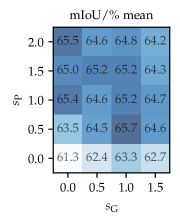
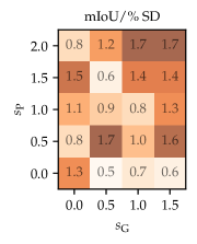
Figure 5: Validation of perturbation strength hyper-parameters on Cityscapes val (mIoU/%). We use 5 different subsets with $1/4$ of the total number of training labels. The hyper-parameters $s_{\text{P}}$ (photometric) and $s_{\text{G}}$ (geometric) are defined in the main text. SD denotes the sample standard deviation.

Figure 6 shows our validation of the consistency loss weight $\alpha$ with SN-RN18 simple-PhTPS. We observe best generalization performance for $\alpha\in[0.25\mkern 1.5mu{..}\mkern 1.5mu0.75]$. We do not scale the learning rate with $(1+\alpha)^{-1}$ because we use a scale-invariant optimization algorithm.

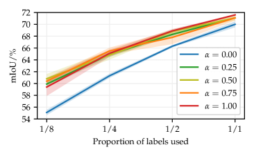
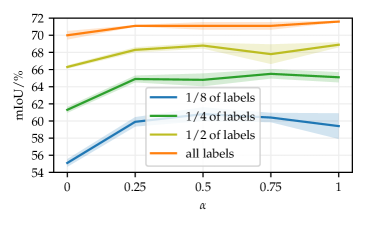
Figure 6: Validation of the consistency loss weight $\alpha$ on Cityscapes val (mIoU/%). We present the same results in two plots with different x-axes: the proportion of labels (left), and the consistency loss weight $\alpha$ (right).

Appendix Bpresents experiments that quantify the effect of updating batch normalization statistics when the inputs are perturbed.

Figure 7 shows qualitative results on the first few validation images with SwiftNet-RN18 trained with $1/4$ of labels. We observe that our method displays a substantial resilience to heavy perturbations like those used during training.

input	ground truth	simple-PhTPS	supervised

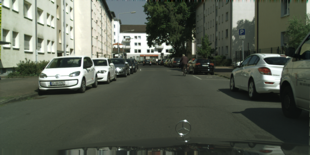
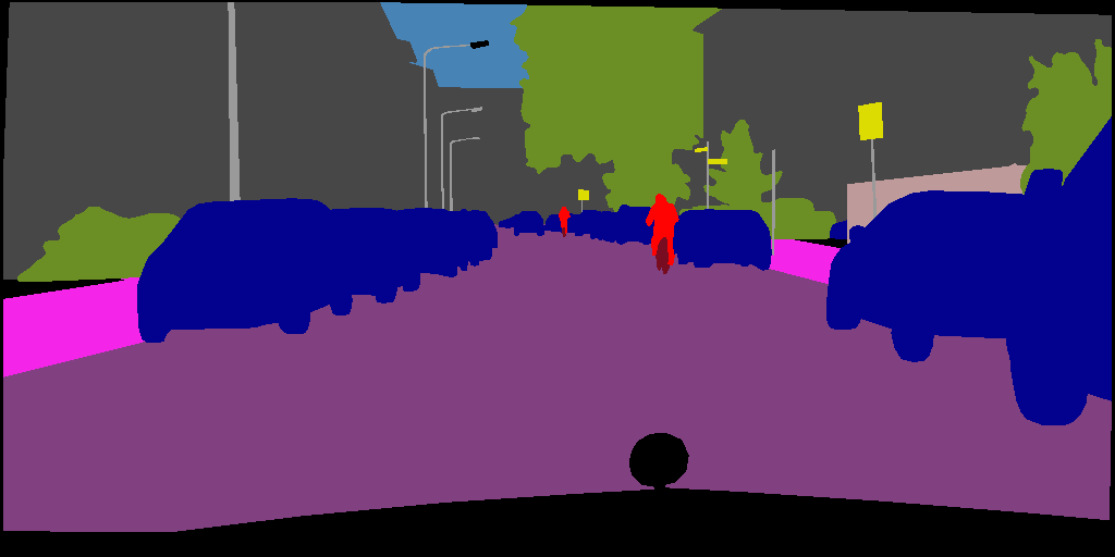
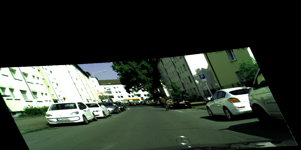
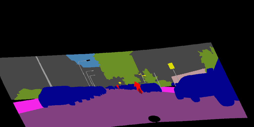
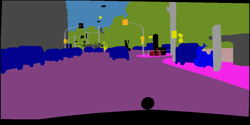
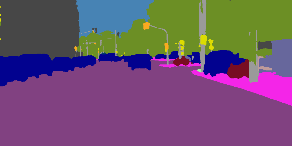
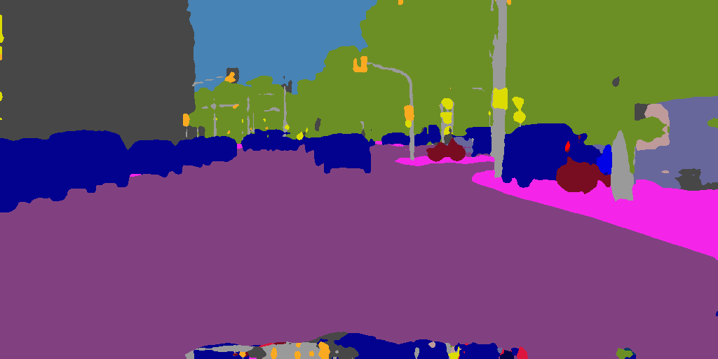
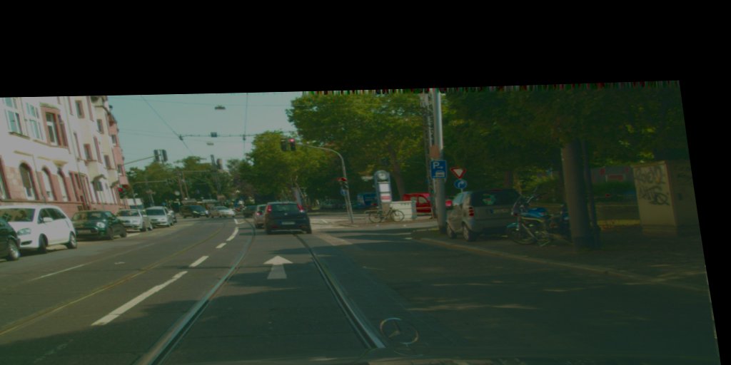
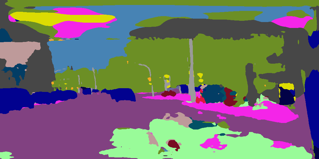
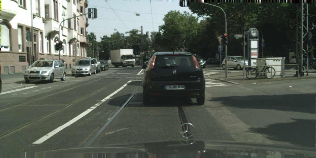
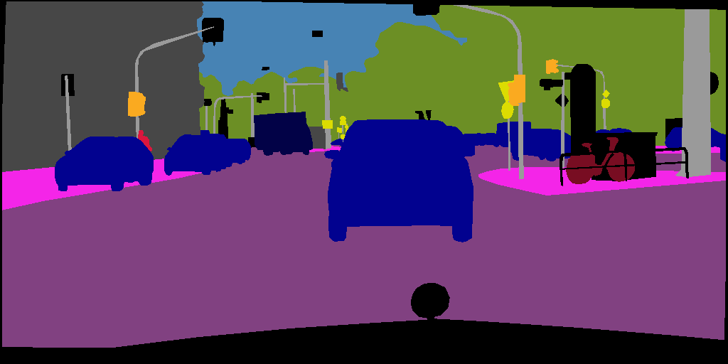
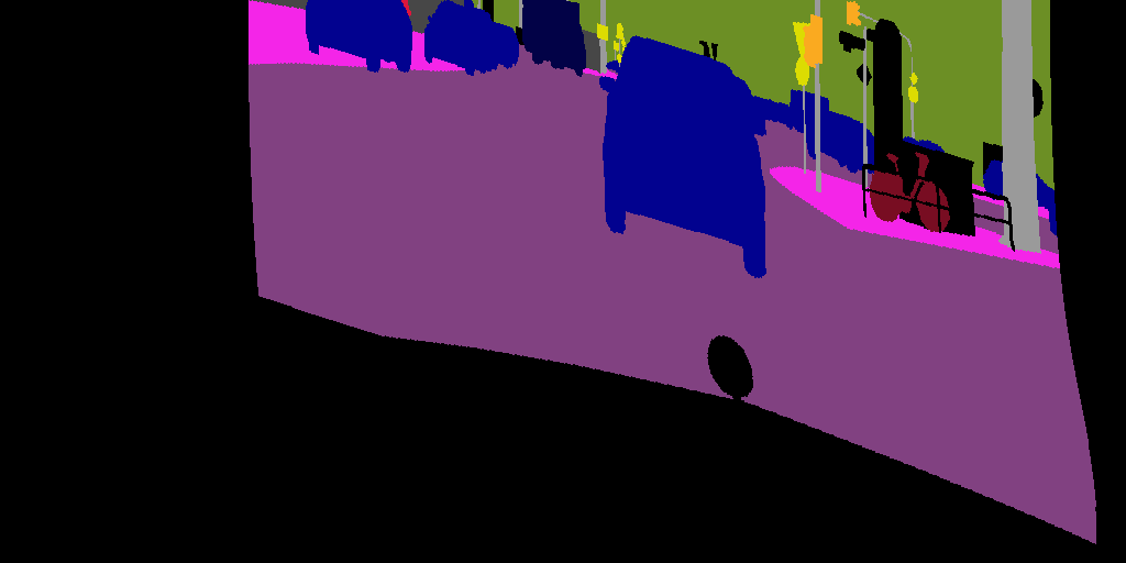
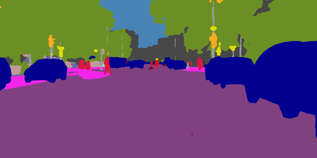
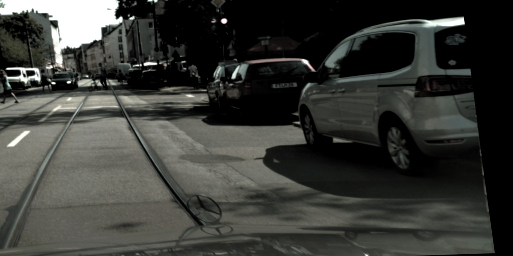
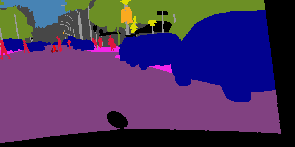
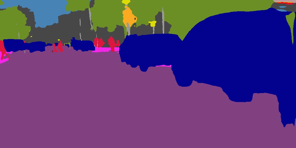
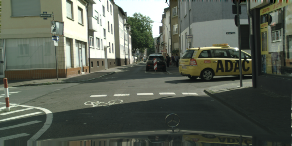
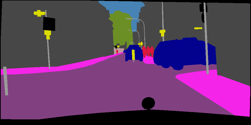
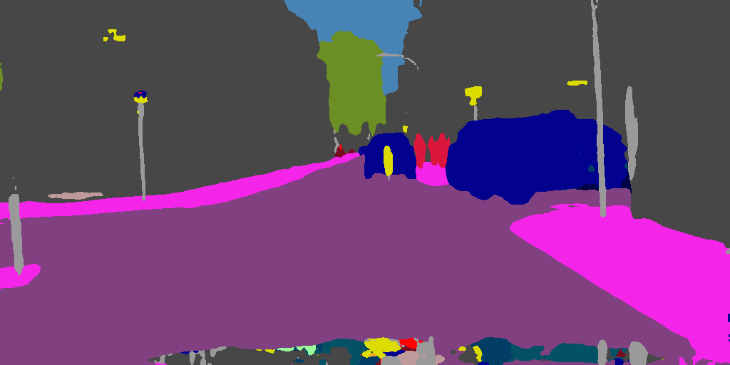
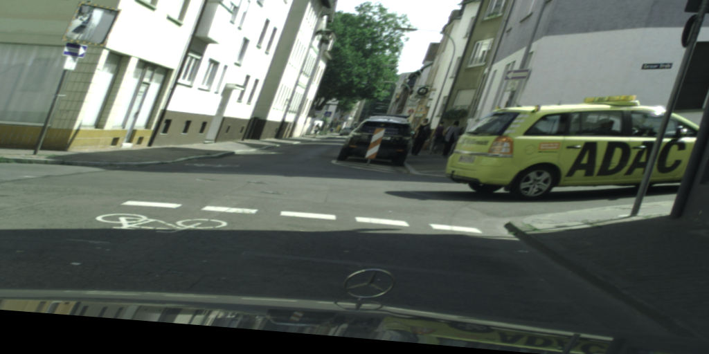
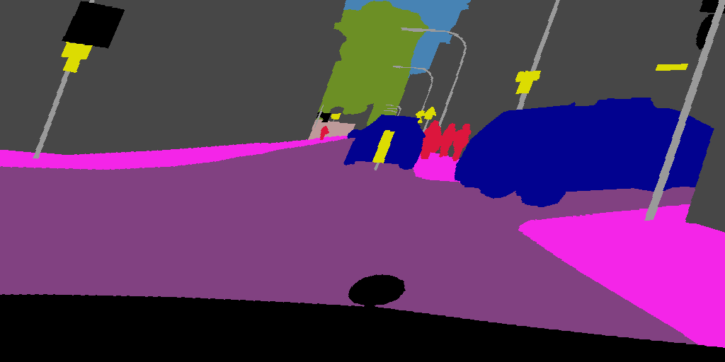
Figure 7: Qualitative results on the first few validation images with SwiftNet-RN18 trained with $1/4$ of half-resolution Cityscapes labels. Odd rows contain unperturbed inputs, and even rows contain PhTPS perturbed inputs. The columns are (left to right): ground truth segmentations, predictions of simple-PhTPS consistency training, and predictions of supervised training.

4.3 Semantic Segmentation on Full-Resolution Cityscapes

Table 3 presents our full resolution experiments in setups like in Table 1, and comparison with previous work. but with full-resolution images and labels. In comparison with KE-GAN [48] and ECS [36], we underperform with $1/8$ labeled images, but outperform with $1/2$ labeled images. Note that KE-GAN [48] also trains on a large text corpus (MIT ConceptNet) as well as that ECS DLv3⁺-RN50 requires 22 GiB of GPU memory with batch size 6 [36], while our SN-RN18 simple-PhTPS requires less than 8 GiB of GPU memory with batch size 8 and can be trained on affordable GPU hardware. Appendix A.2 presents more detailed memory and execution time comparisons with other algorithms.

We note that the concurrent approach DLv3⁺-RN50 CAC [28] outperforms our method with 1/8 and 1/1 labels. However, ResNet-18 has significantly less capacity than ResNet-50. Therefore, the bottom section applies our method to the SwiftNet model with a ResNet-34 backbone, which still has less capacity than ResNet-50. The resulting model outperforms DLv3⁺-RN50 CAC across most configurations. This shows that our method consistently improves when more capacity is available.

We note that training DLv3⁺-RN50 CAC requires three RTX 2080Ti GPUs [28], while our SN-RN34 simple-PhTPS setup requires less than 9 GiB of GPU memory and fits on a single such GPU. Moreover, SN-RN34 has about 4$\times$ faster inference than DLv3⁺-RN50 on RTX 2080Ti.

Table 3: Semi-supervised semantic segmentation performance (mIoU/%) on full-resolution Cityscapes val with different proportions of labeled data. We compare simple-PhTPS and MT-PhTPS (ours) with supervised training and previous work. DLv3⁺-RN50 stands for DeepLab v3⁺ with ResNet-50, and SN for SwiftNet. We run experiments across 5 different dataset splits and report mean mIoUs with standard deviations. Best results overall are bold, and best results within sections are underlined.

Method	Label proportion
	$1/8$	$1/4$	$1/2$	$1/1$
KE-GAN [48]	$66.9_{\phantom{0.0}}$	$70.6_{\phantom{0.0}}$	$72.2_{\phantom{0.0}}$	$75.3_{\phantom{0.0}}$
DLv3+-RN50 supervised [36]	$63.2_{\phantom{0.0}}$	$68.4_{\phantom{0.0}}$	$72.9_{\phantom{0.0}}$	$74.8_{\phantom{0.0}}$
DLv3+-RN50 ECS [36]	$67.4_{\phantom{0.0}}$	$70.7_{\phantom{0.0}}$	$72.9_{\phantom{0.0}}$	$74.8_{\phantom{0.0}}$
DLv3+-RN50 supervised [28]	$63.9_{\phantom{0.0}}$	$68.3_{\phantom{0.0}}$	$71.2_{\phantom{0.0}}$	$76.3_{\phantom{0.0}}$
DLv3+-RN50 CAC [28]	$\mathbf{69.7}_{\phantom{0.0}}$	$\underline{72.7}_{\phantom{0.0}}$	${-}_{\phantom{0.0}}$	$\underline{77.5}_{\phantom{0.0}}$
SN-RN18 supervised	$61.1_{0.4}$	$67.3_{1.1}$	$71.9_{0.1}$	$75.4_{0.4}$
SN-RN18 simple-PhTPS	$66.3_{1.0}$	$71.0_{0.5}$	$\underline{74.3}_{0.7}$	$\underline{75.8}_{0.4}$
SN-RN18 MT-PhTPS	$\underline{68.6}_{0.6}$	$\underline{72.0}_{0.3}$	$73.8_{0.4}$	$75.0_{0.4}$
SN-RN34 supervised	$64.9_{0.8}$	$69.8_{1.0}$	$73.8_{1.4}$	$76.1_{0.8}$
SN-RN34 simple-PhTPS	$69.2_{0.8}$	$73.1_{0.7}$	$\mathbf{76.3}_{0.7}$	$\mathbf{77.9}_{0.2}$
SN-RN34 MT-PhTPS	$\mathbf{70.8}_{1.5}$	$\mathbf{74.3}_{0.5}$	$\mathbf{76.0}_{0.5}$	$77.2_{0.4}$

Finally, we present experiments in the large-data regime where we place the whole fine subset into $\mathbbmsl{D}_{\text{l}}$. In some of these experiments we also train on the large coarsely labeled subset. We denote extent of supervision with subscripts ”l” (labeled) and ”u” (unlabeled). Hence, $\mathrm{C_{\text{u}}}$ in the table denotes the coarse subset without labels. Table 4 investigates the impact of the coarse subset on SwiftNet performance on full-resolution Cityscapes val. We observe that semi-supervised learning brings considerable improvement with respect to fully supervised learning on fine labels only (columns $\mathrm{F_{\text{l}}}$ vs $\mathrm{F_{\text{l}}}\cup\mathrm{C_{\text{u}}}$). It is also interesting to compare the proposed semi-supervised setup ($\mathrm{F_{\text{l}}}\cup\mathrm{C_{\text{u}}}$) with classic fully supervised learning on both subsets ($\mathrm{F_{\text{l}}},\mathrm{C_{\text{l}}}$). We observe that semi-supervised learning with SwiftNet-RN18 comes close to supervised learning with coarse labels. Moreover, semi-supervised learning prevails when we plug in SwiftNet-RN34. These experiments suggest that semi-supervised training represents an attractive alternative to coarse labels and large annotation efforts.

Table 4: Effects of an additional large dataset on supervised and semi-supervised learning on full-resolution Cityscapes val (mIoU/%). Tags F and C denote fine and coarse subsets, respectively. Subset indices denote whether we train with labels (l) or one-way consistency (u).

Method	$\mathrm{F_{\text{l}}}$	$(\mathrm{F_{\text{l}}},\mathrm{F_{\text{u}}})$	$(\mathrm{F_{\text{l}}},\mathrm{F_{\text{u}}}\cup\mathrm{C_{\text{u}}})$	$(\mathrm{F_{\text{l}}},\mathrm{C_{\text{l}}})$
SN-RN18 simple-PhTPS	$75.4_{0.4}$	$75.8_{0.4}$	$76.5_{0.3}$	$\mathbf{76.9}_{0.3}$
SN-RN18 MT-PhTPS		$75.0_{0.4}$	$75.5_{0.3}$
SN-RN34 simple-PhTPS	$76.1_{0.8}$	$77.9_{0.2}$	$\mathbf{78.5}_{0.4}$	$77.7_{0.4}$

4.4 Validation of Consistency Variants

Table 5 presents experiments with supervised baselines and four variants of semi-supervised consistency training. All semi-supervised experiments use the same PhTPS perturbations on CIFAR-10 (4000 labels and 50000 images) and half-resolution Cityscapes (the SwiftNet-RN18 setups with $1/4$ labels from Table 1). We investigate the following kinds of consistency: one-way with clean teacher (1w-ct, cf. Figure 1(c)), one-way with clean student (1w-cs, cf. Figure 1(b)), two-way with one clean input (2w-c1, cf. Figure 1(d)), and one-way with both inputs perturbed (1w-p2). Note that two-way consistency is not possible with Mean Teacher. Also, when both inputs are perturbed (1w-p2), we have to use the inverse geometric transformation on dense predictions [3]. We achieve that by forward warping [40] with the same displacement field. Two-way consistency with both inputs perturbed (2w-p2) is possible as well. We expect it to behave similarly to 1w-2p because it could be seen as a superposition of two opposite one-way consistencies, and our preliminary experiments suggest so.

We observe that 1w-ct outperforms all other variants, while 2w-c1 performs in-between 1w-ct and 1w-cs. This confirms our hypothesis that predictions in clean inputs make better consistency targets. We note that 1w-p2 often outperforms 1w-cs, while always underperforming with respect to 1w-ct. A closer inspection suggests that 1w-p2 sometimes learns to cheat the consistency loss by outputting similar predictions for all perturbed images. This occurs more often when batch normalization uses the batch statistics estimated during training. A closer inspection of 1w-cs experiments on Cityscapes indicates consistency cheating combined with severe overfitting to the training dataset.

Table 5: Comparison of 4 consistency variants under PhTPS perturbations: one-way with clean teacher (1w-ct), one-way with clean student (1w-cs), two-way with one input clean (2w-c1), and one-way with both inputs perturbed (1w-p2). Algorithms are evaluated on CIFAR-10 test (accuracy/%) while training on 4000 out of 50000 labels (CIFAR-10, $2/25$) and half-resolution Cityscapes val (mIoU/%) while training on $1/4$ of labels from Cityscapes train with SwiftNet-RN18 (CS-half, $1/4$).

Dataset	Method	sup.	1w-ct	1w-cs	2w-c1	1w-p2
CIFAR-10, 4k	WRN-28-2 simple-PhTPS	$80.8_{0.4}$	$\mathbf{90.8}_{0.3}$	$69.3_{4.2}$	$72.9_{2.6}$	$73.3_{7.0}$
CIFAR-10, 4k	WRN-28-2 MT-PhTPS	$80.8_{0.4}$	$\mathbf{90.8}_{0.4}$	$80.5_{0.5}$	-	$73.4_{1.4}$
CS-half, 1/4	SN-RN18 simple-PhTPS	$61.5_{0.5}$	$\mathbf{65.3}_{1.9}$	$\phantom{0}1.6_{1.0}$	$16.7_{3.0}$	$61.6_{0.5}$
CS-half, 1/4	SN-RN18 MT-PhTPS	$61.5_{0.5}$	$\mathbf{66.0}_{1.0}$	$61.5_{1.4}$	-	$62.0_{1.1}$

4.5 Image Classification on CIFAR-10

Table 6 evaluates image classification performance of two supervised baselines and 4 semi-supervised algorithms on CIFAR-10. The first supervised baseline uses only labeled data with standard data augmentation. The second baseline additionally uses our perturbations for data augmentation. The third algorithm is VAT with entropy minimization [38]. The simple-PhTPS approach outperforms supervised approaches and VAT. Again, two-way consistency results in the worst generalization performance. Perturbing the teacher input results in accuracy below 17% for 4000 or less labeled examples, and is not displayed. Note that somewhat better performance can be achieved by complementing consistency with other techniques that are either unsuitable for dense prediction or out of scope of this paper [11, 65, 1].

Table 6: Classification accuracy [%] on CIFAR-10 test with WRN-28-2. We compare two supervised approaches (top), VAT with entropy minimization [38] (middle), and two-way and one-way consistency with our perturbations (bottom three rows). We report means and standard deviations of $5$ runs. The label ”supervised PhTPS-aug” denotes supervised training where half of each mini-batch is perturbed with PhTPS.

Method	Number of labeled examples
	250	1000	4000	50000
supervised	$31.8_{0.6}$	$59.3_{1.4}$	$81.0_{0.2}$	$94.7$
supervised PhTPS-aug	$48.7_{0.9}$	$67.2_{0.5}$	$81.7_{0.2}$	$95.0$
VAT + entropy minimization	$41.0_{2.5}$	$73.2_{1.5}$	$84.2_{0.4}$	$90.5_{0.2}$
1w-cs simple-PhTPS	$27.7_{5.9}$	$51.7_{3.5}$	$69.3_{4.2}$	$91.6_{1.5}$
2w-c1 simple-PhTPS	$30.3_{1.8}$	$54.8_{1.5}$	$72.9_{2.6}$	$95.9_{0.2}$
1w-ct simple-PhTPS	$\mathbf{68.8}_{5.4}$	$\mathbf{84.2}_{0.4}$	$\mathbf{90.6}_{0.4}$	$\mathbf{96.2}_{0.2}$

5 Discussion

We have presented the first comprehensive study of one-way consistency for semi-supervised dense prediction, and proposed a novel perturbation model which leads to competitive generalization performance on Cityscapes. Our study clearly shows that one-way consistency with clean teacher outperforms other forms of consistency (e.g. clean student or two-way) both in terms of generalization performance and training footprint. We explain this by observing that predictions in perturbed images tend to be less reliable targets.

The proposed perturbation model is a composition of a photometric transformation and a geometric warp. These two kinds of perturbations have to be treated differently since we desire invariance to the former and equivariance to the latter. Our perturbation model outperforms CutMix both in standard experiments with DeepLabv2-RN101 and in combination with recent efficient models (SwiftNet-RN18 and SwiftNet-RN34).

We consider two teacher formulations. In the simple formulation the teacher is a frozen copy of the student. In the Mean Teacher formulation, the teacher is a moving average of student parameters. Mean Teacher outperforms simple consistency in low data regimes (half resolution, few labels). However, experiments with more data suggest that the simple one-way formulation scales significantly better.

To the best of our knowledge, this is the first account of semi-supervised semantic segmentation with efficient models. This combination is essential for many practical real-time applications where there is a lack of large datasets with suitable pixel-level groundtruth. Many of our experiments are based on SwiftNet-RN18, which behaves similarly to DeepLabv2-RN101, while offering about 9$\times$ faster inference on half-resolution images, and about 15$\times$ faster inference on full-resolution images on RTX 2080Ti. Experiments on Cityscapes coarse reveal that semi-supervised learning with one-way consistency can come close and exceed full supervision with coarse annotations. Simplicity, competitive performance and speed of training make this approach a very attractive baseline for evaluating future semi-supervised approaches in the dense prediction context.

Appendix A Additional Algorithm Comparisons

A.1 Hyper-Parameters

Tables 7 and 8 review hyper-parameters of consistency-based semi-supervised algorithms from Tables 1 and  3.

Table 7: Overview of hyper-parameters of consistency-based algorithms for semi-supervised semantic segmentation. We denote the setup that we use in our experiments including supervised training with “our”. We use the following symbols: $\bm{y}$ is the teacher prediction, $\vphantom{\bm{y}}\smash[t]{\tilde{\bm{y}}}$ is the student prediction, $\mathrm{hard}$ is a function that maps a vector representing a distribution to the closest one-hot vector ($\mathrm{hard}_{[c]}={\mathinner{\left\llbracket{c=\operatorname*{arg\,max}_{k}\bm{y}_{[k]}}\right\rrbracket}}$), $e$ is the proportion of completed epochs, $\alpha$ is the consistency loss weight, and $\eta$ is the base learning rate. The if-clause in the “Consistency loss” column represents confidence thresholding, i.e., determines whether the pixel is included in loss computation.

Model	Method	Crop Size	Jitter. Scale	Iterations	Epochs	$B_{l}$	$B_{u}$	Consistency Loss	$\alpha$	Learning Rate
DLv2	MT-CutMix [14]	321	$[0.5\mkern 1.5mu{..}\mkern 1.5mu1.5]$	40,000	135 *	10	10	$\|\mathrm{hard}(\bm{y})-\vphantom{\bm{y}}\smash[t]{\tilde{\bm{y}}}\|_{2}^{2}$ if $\max_{c}\bm{y}_{[c]}>0.97$	0.5	$\eta(1-e)^{0.9}$
DLv2	MT-CutMix$\sim$[14]	321	$[0.5\mkern 1.5mu{..}\mkern 1.5mu1.5]$	37,100	100	4	4	$\|\mathrm{hard}(\bm{y})-\vphantom{\bm{y}}\smash[t]{\tilde{\bm{y}}}\|_{2}^{2}$ if $\max_{c}\bm{y}_{[c]}>0.97$	1	$\eta(1-e)^{0.9}$
DLv2	ours	448	$[0.5\mkern 1.5mu{..}\mkern 1.5mu2]$	74,200	200	4	4	$\mathit{D}(\bm{y},\vphantom{\bm{y}}\smash[t]{\tilde{\bm{y}}})$	0.5	$\eta(1-e)^{0.9}$
SN	ours	448	$[0.5\mkern 1.5mu{..}\mkern 1.5mu2]$	74,200	200	8	8	$\mathit{D}(\bm{y},\vphantom{\bm{y}}\smash[t]{\tilde{\bm{y}}})$	0.5	$\eta\cos(e\pi/2)$
SN	ours	768	$[0.5\mkern 1.5mu{..}\mkern 1.5mu2]$	92,750	250	8	8	$\mathit{D}(\bm{y},\vphantom{\bm{y}}\smash[t]{\tilde{\bm{y}}})$	0.5	$\eta\cos(e\pi/2)$
DLv3+	CAC [28]	720	$[0.5\mkern 1.5mu{..}\mkern 1.5mu1.5]$	92,560	249 *	8	8	see [28]	${\mathinner{\left\llbracket{e>5/80}\right\rrbracket}}\cdot 0.1$	$\eta(1-e)^{0.9}$
DLv3+	ours	720	$[0.5\mkern 1.5mu{..}\mkern 1.5mu1.5]$	92,560	249 *	8	8	$\mathit{D}(\bm{y},\vphantom{\bm{y}}\smash[t]{\tilde{\bm{y}}})$	0.5	$\eta(1-e)^{0.9}$

^∗ Some authors [14, 28] use the word “epoch” to refer to a fixed number of iterations — 1000 and 1157 iterations, respectively.

Table 8: Optimizer hyper-parameter configurations for Cityscapes semantic segmentation experiments, represented in a PyTorch-like style.

Model	Method	Optimizer Configuration
		Main	Backbone (Difference)
DLv2	MT-CutMix [14]	SGD, lr=$3\cdot 10^{-5}$, momentum=$0.9$, weight_decay=$5\cdot 10^{-4}$
DLv2	MT-CutMix$\sim$[14]	SGD, lr=$3\cdot 10^{-5}$, momentum=$0.9$, weight_decay=$5\cdot 10^{-4}$
DLv2	ours	Adam, betas=$(0.9,0.99)$, lr=$4\cdot 10^{-4}$, weight_decay=$1\cdot 10^{-4}$	lr=$1\cdot 10^{-4}$, weight_decay=$2.5\cdot 10^{-5}$
SN	ours	Adam, betas=$(0.9,0.99)$, lr=$4\cdot 10^{-4}$, weight_decay=$2.5\cdot 10^{-5}$	lr=$1\cdot 10^{-4}$, weight_decay=$6.25\cdot 10^{-6}$
DLv3+	CAC [28]	SGD, lr=$1\cdot 10^{-1}$, momentum=$0.9$	lr=$1\cdot 10^{-2}$, weight_decay=$1\cdot 10^{-4}$
DLv3+	ours	SGD, lr=$1\cdot 10^{-1}$, momentum=$0.9$	lr=$1\cdot 10^{-2}$, weight_decay=$1\cdot 10^{-4}$

A.2 Time and Memory Performance Characteristics

Table 9 shows memory requirements and training times of methods from Tables 1 and 3. The times include data loading and processing, and do not include evaluation on the validation set. The memory measurements are based on the max_memory_allocated and reset_peak_memory_stats procedures from the torch.cuda package. Some algorithms did not fit into the memory of GTX 2080Ti. The memory allocations are higher than in Figure 4 because the supervised prediction, perturbed inputs, and perturbed outputs are unnecessarily kept in memory.

For DeepLabv3⁺-RN50, we use the number of iterations, batch size, and crop size from [28]. Note, however, that the method from [28] has the memory requirements of two-way consistency because of per-pixel directionality.

Table 9: Half resolution Cityscapes (top section) and Cityscapes (bottom section) maximum memory allocation and training time on two GPUs.

Model	Method	Crop Size	Iterations	$B_{l}$	$B_{u}$	Memory $/\mathrm{MiB}$	Duration$/\mathrm{min}$
							A4500	2080Ti
DLv2-RN101	MT-CutMix [14]	321	40000	10	10	16289	1067	–
	MT-CutMix$\sim$[14]	321	37100	4	4	7037	794	1314
DLv2-RN101	supervised	448	74300	4	–	6611	338	602
	MT-PhTPS	448	74300	4	4	7021	816	1397
SN-RN18	supervised	448	74200	4	–	1646	119	161
	simple-PhTPS	448	74200	8	8	2398	228	279
	MT-PhTPS	448	74200	8	8	2456	234	297
SN-RN18	supervised	768	92750	8	–	4444	321	432
	simple-PhTPS	768	92750	8	8	6683	732	963
	MT-PhTPS	768	92750	8	8	6727	768	965
SN-RN34	supervised	768	92750	8	–	5500	422	570
	simple-PhTPS	768	92750	8	8	7737	994	1268
	MT-PhTPS	768	92750	8	8	7818	1013	1276
DLv3+-RN50	supervised	720	92560	8	–	11645	1229	–
	simple-PhTPS	720	92560	8	8	13384	1884	–
	CAC [28]	720	92560	8	8	25165†	$>$3000∗	–

^† The original implementation requires 36005 MiB. Approximately 10.6 GiB can be saved by accumulating gradients as in Algorithm LABEL:alg:training.
^∗ Estimated by running on NVidia A100.

Table 10 shows the numbers of model parameters, and Table 11 shows inference speeds of models from Tables 1 and 3.

Table 10: Number of model parameters.

Model	Number of parameters
DeepLabv2-RN101	$43.80\cdot 10^{6}$
DeepLabv3+-RN50	$40.35\cdot 10^{6}$
SwiftNet-RN34	$21.91\cdot 10^{6}$
SwiftNet-RN18	$11.80\cdot 10^{6}$

Table 11: Model inference speed (number of iterations per second) on three different GPUs and two input resolutions. Inputs are processed one by one, without overlap in computation. The measurements include the computation of the cross-entropy loss, but do not include data loading and preparation.

	$1024\times 2048$			$512\times 1024$
	A4500	2080Ti	1080Ti	A4500	2080Ti	1080Ti
DeepLabv2-RN101	5.1	3.0	1.5	19.6	12.2	6.3
DeepLabv3+-RN50	16.1	9.6	5.2	54.2	30.7	23.5
SwiftNet-RN34	39.2	30.5	23.6	93.4	86.1	73.5
SwiftNet-RN18	56.5	45.3	34.6	139.5	115.8	98.4

Appendix B Effect of Updating Batch Normalization Statistics in the Perturbed Student

Batch normalization layers estimate population statistics during training as exponential moving averages. Training on perturbed images can adversely affect suitability of these estimates. Consequently, we explore the design choice to update the statistics only on clean inputs (when the supervised loss is computed), instead of both on clean and on perturbed inputs.

Note that this configuration difference does not affect parameter optimization because the training always relies on mini-batch statistics.. Figure 8 shows the effect of disabling the updates of batch normalization statistics when the model instance (student) receives perturbed inputs in our semi-supervised training (one way consistency with clean teacher). The experiments are conducted according to the corresponding descriptions in section 4. In case of half-resolution Cityscapes, disabling updates in the perturbed student (blue) increased the validation mIoU by between $0.3$ and $1.4$ pp, depending on the proportion of labels. However, in case of full-resolution Cityscapes, an opposite effect occured – mIoU decreased by between $0.1$ and $1.1$ pp. In CIFAR-10 experiments, the effect is mostly neutral.

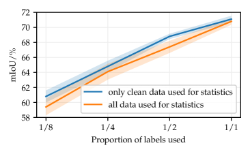
(a) Half-resolution Cityscapes val.

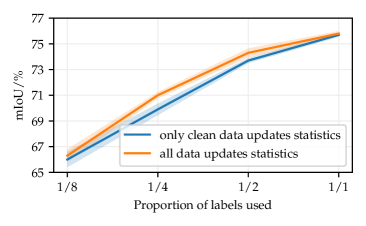
(b) Cityscapes val.

(c) CIFAR-10 validation set.

Figure 8: Effect of updating batch normalization statistics in the perturbed student.

References

- [1] David Berthelot, Nicholas Carlini, Ian Goodfellow, Nicolas Papernot, Avital Oliver, and Colin A Raffel. Mixmatch: A holistic approach to semi-supervised learning. In Advances in Neural Information Processing Systems 32, pages 5049–5059. Curran Associates, Inc., 2019.
- [2] Fred L. Bookstein. Principal warps: Thin-plate splines and the decomposition of deformations. IEEE Trans. Pattern Anal. Mach. Intell., 11(6):567–585, 1989.
- [3] Gerda Bortsova, Florian Dubost, Laurens Hogeweg, Ioannis Katramados, and Marleen de Bruijne. Semi-supervised medical image segmentation via learning consistency under transformations. In MICCAI, 2019.
- [4] Olivier Chapelle, Bernhard Schlkopf, and Alexander Zien. Semi-Supervised Learning. The MIT Press, 1st edition, 2010.
- [5] Liang-Chieh Chen, Raphael Gontijo Lopes, Bowen Cheng, Maxwell D. Collins, Ekin D. Cubuk, Barret Zoph, Hartwig Adam, and Jonathon Shlens. Naive-student: Leveraging semi-supervised learning in video sequences for urban scene segmentation. In Andrea Vedaldi, Horst Bischof, Thomas Brox, and Jan-Michael Frahm, editors, Computer Vision - ECCV 2020 - 16th European Conference, Glasgow, UK, August 23-28, 2020, Proceedings, Part IX, volume 12354 of Lecture Notes in Computer Science, pages 695–714. Springer, 2020.
- [6] Liang-Chieh Chen, George Papandreou, Iasonas Kokkinos, Kevin Murphy, and Alan L. Yuille. Deeplab: Semantic image segmentation with deep convolutional nets, atrous convolution, and fully connected crfs. IEEE Trans. Pattern Anal. Mach. Intell., 40(4):834–848, 2018.
- [7] Liang-Chieh Chen, George Papandreou, Iasonas Kokkinos, Kevin Murphy, and Alan L. Yuille. Deeplab: Semantic image segmentation with deep convolutional nets, atrous convolution, and fully connected crfs. IEEE Transactions on Pattern Analysis and Machine Intelligence, 40(4):834–848, 2018.
- [8] Xinlei Chen and Kaiming He. Exploring simple siamese representation learning. In IEEE Conference on Computer Vision and Pattern Recognition, CVPR 2021, virtual, June 19-25, 2021, pages 15750–15758. Computer Vision Foundation / IEEE, 2021.
- [9] Jang Hyun Cho, Utkarsh Mall, Kavita Bala, and Bharath Hariharan. Picie: Unsupervised semantic segmentation using invariance and equivariance in clustering. In CVPR, 2021.
- [10] Marius Cordts, Mohamed Omran, Sebastian Ramos, Timo Scharwächter, Markus Enzweiler, Rodrigo Benenson, Uwe Franke, Stefan Roth, and Bernt Schiele. The cityscapes dataset. In CVPRW, 2015.
- [11] Ekin Dogus Cubuk, Barret Zoph, Jonathon Shlens, and Quoc Le. Randaugment: Practical automated data augmentation with a reduced search space. In Hugo Larochelle, Marc’Aurelio Ranzato, Raia Hadsell, Maria-Florina Balcan, and Hsuan-Tien Lin, editors, Advances in Neural Information Processing Systems 33: Annual Conference on Neural Information Processing Systems 2020, NeurIPS 2020, December 6-12, 2020, virtual, 2020.
- [12] Alexey Dosovitskiy, Jost Tobias Springenberg, Martin Riedmiller, and Thomas Brox. Discriminative unsupervised feature learning with convolutional neural networks. In Advances in neural information processing systems, pages 766–774, 2014.
- [13] Jean Duchon. Splines minimizing rotation-invariant semi-norms in sobolev spaces. In Constructive theory of functions of several variables, pages 85–100. Springer, 1977.
- [14] Geoffrey French, Samuli Laine, Timo Aila, Michal Mackiewicz, and Graham Finlayson. Semi-supervised semantic segmentation needs strong, varied perturbations. In BMVC, 2020.
- [15] Hongmin Gao, Dan Yao, Mingxia Wang, Chenming Li, Haiyun Liu, Zaijun Hua, and Jiawei Wang. A hyperspectral image classification method based on multi-discriminator generative adversarial networks. Sensors, 19(15), 2019.
- [16] Jan E. Gerken, Jimmy Aronsson, Oscar Carlsson, Hampus Linander, Fredrik Ohlsson, Christoffer Petersson, and Daniel Persson. Geometric deep learning and equivariant neural networks. CoRR, abs/2105.13926, 2021.
- [17] Yves Grandvalet and Yoshua Bengio. Semi-supervised learning by entropy minimization. In L. K. Saul, Y. Weiss, and L. Bottou, editors, Advances in Neural Information Processing Systems, pages 529–536. MIT Press, 2005.
- [18] Jean-Bastien Grill, Florian Strub, Florent Altché, Corentin Tallec, Pierre Richemond, Elena Buchatskaya, Carl Doersch, Bernardo Avila Pires, Zhaohan Guo, Mohammad Gheshlaghi Azar, Bilal Piot, koray kavukcuoglu, Remi Munos, and Michal Valko. Bootstrap your own latent - a new approach to self-supervised learning. In H. Larochelle, M. Ranzato, R. Hadsell, M. F. Balcan, and H. Lin, editors, Advances in Neural Information Processing Systems, volume 33, pages 21271–21284. Curran Associates, Inc., 2020.
- [19] Ivan Grubišić, Marin Oršić, and Siniša Šegvić. A baseline for semi-supervised learning of efficient semantic segmentation models. In 17th International Conference on Machine Vision and Applications, MVA 2021, Aichi, Japan, July 25-27, 2021, pages 1–5. IEEE, 2021.
- [20] Philip Häusser, Alexander Mordvintsev, and Daniel Cremers. Learning by association - A versatile semi-supervised training method for neural networks. In 2017 IEEE Conference on Computer Vision and Pattern Recognition, CVPR 2017, Honolulu, HI, USA, July 21-26, 2017, pages 626–635. IEEE Computer Society, 2017.
- [21] Kaiming He, Haoqi Fan, Yuxin Wu, Saining Xie, and Ross Girshick. Momentum contrast for unsupervised visual representation learning. In 2020 IEEE/CVF Conference on Computer Vision and Pattern Recognition (CVPR), pages 9726–9735, 2020.
- [22] Gao Huang, Zhuang Liu, Geoff Pleiss, Laurens van der Maaten, and Kilian Q. Weinberger. Convolutional networks with dense connectivity. IEEE Trans. Pattern Anal. Mach. Intell., 44(12):8704–8716, 2022.
- [23] Wei-Chih Hung, Yi-Hsuan Tsai, Yan-Ting Liou, Yen-Yu Lin, and Ming-Hsuan Yang. Adversarial learning for semi-supervised semantic segmentation. In BMVC, page 65, 2018.
- [24] Dong hyun Lee. Pseudo-label: The simple and efficient semi-supervised learning method for deep neural networks. In ICMLW, 2013.
- [25] Alexander Kolesnikov, Xiaohua Zhai, and Lucas Beyer. Revisiting self-supervised visual representation learning. In IEEE Conference on Computer Vision and Pattern Recognition, CVPR 2019, Long Beach, CA, USA, June 16-20, 2019, pages 1920–1929. Computer Vision Foundation / IEEE, 2019.
- [26] Ivan Krešo, Josip Krapac, and Siniša Šegvić. Efficient ladder-style densenets for semantic segmentation of large images. IEEE Transactions on Intelligent Transportation Systems, 2020.
- [27] Alex Kurakin, Chun-Liang Li, Colin Raffel, David Berthelot, Ekin Dogus Cubuk, Han Zhang, Kihyuk Sohn, Nicholas Carlini, and Zizhao Zhang. Fixmatch: Simplifying semi-supervised learning with consistency and confidence. In NeurIPS, 2020.
- [28] Xin Lai, Zhuotao Tian, Li Jiang, Shu Liu, Hengshuang Zhao, Liwei Wang, and Jiaya Jia. Semi-supervised semantic segmentation with directional context-aware consistency. In CVPR, 2021.
- [29] Samuli Laine and Timo Aila. Temporal ensembling for semi-supervised learning. In 5th International Conference on Learning Representations, ICLR 2017, Toulon, France, April 24-26, 2017, Conference Track Proceedings. OpenReview.net, 2017.
- [30] Jungbeom Lee, Eunji Kim, Sungmin Lee, Jangho Lee, and Sungroh Yoon. Ficklenet: Weakly and semi-supervised semantic image segmentation using stochastic inference. In IEEE Conference on Computer Vision and Pattern Recognition, CVPR 2019, Long Beach, CA, USA, June 16-20, 2019, pages 5267–5276. Computer Vision Foundation / IEEE, 2019.
- [31] Karel Lenc and Andrea Vedaldi. Understanding image representations by measuring their equivariance and equivalence. Int. J. Comput. Vision, 127(5):456–476, may 2019.
- [32] Jonathan Long, Evan Shelhamer, and Trevor Darrell. Fully convolutional networks for semantic segmentation. In 2015 IEEE Conference on Computer Vision and Pattern Recognition (CVPR), pages 3431–3440, 2015.
- [33] Ilya Loshchilov and Frank Hutter. SGDR: stochastic gradient descent with warm restarts. In 5th International Conference on Learning Representations, ICLR 2017, Toulon, France, April 24-26, 2017, Conference Track Proceedings. OpenReview.net, 2017.
- [34] Emmanuel Maggiori, Yuliya Tarabalka, Guillaume Charpiat, and Pierre Alliez. Can semantic labeling methods generalize to any city? the inria aerial image labeling benchmark. In 2017 IEEE International Geoscience and Remote Sensing Symposium, IGARSS 2017, Fort Worth, TX, USA, July 23-28, 2017, pages 3226–3229. IEEE, 2017.
- [35] David McClosky, Eugene Charniak, and Mark Johnson. Effective self-training for parsing. In Proceedings of the Human Language Technology Conference of the NAACL, Main Conference, pages 152–159, New York City, USA, 6 2006. Association for Computational Linguistics.
- [36] Robert Mendel, Luis Souza Jr, David Rauber, João Papa, and Christoph Palm. Semi-supervised segmentation based on error-correcting supervision. In ECCV, 2020.
- [37] S. Mittal, M. Tatarchenko, and T. Brox. Semi-supervised semantic segmentation with high- and low-level consistency. IEEE Transactions on Pattern Analysis and Machine Intelligence, pages 1–1, 2019.
- [38] Takeru Miyato, Shin-ichi Maeda, Masanori Koyama, and Shin Ishii. Virtual adversarial training: A regularization method for supervised and semi-supervised learning. IEEE Trans. Pattern Anal. Mach. Intell., 41(8):1979–1993, 2019.
- [39] Gerhard Neuhold, Tobias Ollmann, Samuel Rota Bulò, and Peter Kontschieder. Mapillary vistas dataset for semantic understanding of street scenes. In ICCV, pages 5000–5009, 2017.
- [40] Simon Niklaus and Feng Liu. Softmax splatting for video frame interpolation. In IEEE Conference on Computer Vision and Pattern Recognition, 2020.
- [41] Christopher Olah. Visual information theory, 2015.
- [42] Avital Oliver, Augustus Odena, Colin A Raffel, Ekin Dogus Cubuk, and Ian Goodfellow. Realistic evaluation of deep semi-supervised learning algorithms. In S. Bengio, H. Wallach, H. Larochelle, K. Grauman, N. Cesa-Bianchi, and R. Garnett, editors, Advances in Neural Information Processing Systems, volume 31. Curran Associates, Inc., 2018.
- [43] Marin Oršić, Ivan Krešo, Petra Bevandić, and Siniša Šegvić. In defense of pre-trained imagenet architectures for real-time semantic segmentation of road-driving images. In Proceedings of the IEEE conference on computer vision and pattern recognition, pages 12607–12616, 2019.
- [44] Marin Oršić and Siniša Šegvić. Efficient semantic segmentation with pyramidal fusion. Pattern Recognition, 110:107611, 2021.
- [45] Yassine Ouali, Céline Hudelot, and Myriam Tami. Semi-supervised semantic segmentation with cross-consistency training. In 2020 IEEE/CVF Conference on Computer Vision and Pattern Recognition, CVPR 2020, Seattle, WA, USA, June 13-19, 2020. IEEE, 2020.
- [46] Adam Paszke, Sam Gross, Francisco Massa, Adam Lerer, James Bradbury, Gregory Chanan, Trevor Killeen, Zeming Lin, Natalia Gimelshein, Luca Antiga, Alban Desmaison, Andreas Kopf, Edward Yang, Zachary DeVito, Martin Raison, Alykhan Tejani, Sasank Chilamkurthy, Benoit Steiner, Lu Fang, Junjie Bai, and Soumith Chintala. Pytorch: An imperative style, high-performance deep learning library. In Advances in Neural Information Processing Systems 32, pages 8024–8035. Curran Associates, Inc., 2019.
- [47] Gaurav Patel and Jose Dolz. Weakly supervised segmentation with cross-modality equivariant constraints. Medical Image Anal., 77:102374, 2022.
- [48] Mengshi Qi, Yunhong Wang, Jie Qin, and Annan Li. Ke-gan: Knowledge embedded generative adversarial networks for semi-supervised scene parsing. In Proceedings of the IEEE Conference on Computer Vision and Pattern Recognition, pages 5237–5246, 2019.
- [49] Siyuan Qiao, Wei Shen, Zhishuai Zhang, Bo Wang, and Alan Yuille. Deep co-training for semi-supervised image recognition. In Proceedings of the european conference on computer vision (eccv), pages 135–152, 2018.
- [50] Antti Rasmus, Mathias Berglund, Mikko Honkala, Harri Valpola, and Tapani Raiko. Semi-supervised learning with ladder networks. In Advances in Neural Information Processing Systems 28: Annual Conference on Neural Information Processing Systems 2015, December 7-12, 2015, Montreal, Quebec, Canada, pages 3546–3554, 2015.
- [51] Olaf Ronneberger, Philipp Fischer, and Thomas Brox. U-net: Convolutional networks for biomedical image segmentation. In Nassir Navab, Joachim Hornegger, William M. Wells III, and Alejandro F. Frangi, editors, Medical Image Computing and Computer-Assisted Intervention - MICCAI 2015 - 18th International Conference Munich, Germany, October 5 - 9, 2015, Proceedings, Part III, volume 9351 of Lecture Notes in Computer Science, pages 234–241, 2015.
- [52] Samuel Rota Bulò, Lorenzo Porzi, and Peter Kontschieder. In-place activated batchnorm for memory-optimized training of DNNs. In CVPR, June 2018.
- [53] Mehdi Sajjadi, Mehran Javanmardi, and Tolga Tasdizen. Mutual exclusivity loss for semi-supervised deep learning. In Advances in Neural Information Processing Systems 29: Annual Conference on Neural Information Processing Systems 2016, December 5-10, 2016, Barcelona, Spain, pages 1163–1171. IEEE, 2016.
- [54] Tim Salimans, Ian J. Goodfellow, Wojciech Zaremba, Vicki Cheung, Alec Radford, and Xi Chen. Improved techniques for training gans. In Advances in Neural Information Processing Systems 29: Annual Conference on Neural Information Processing Systems 2016, December 5-10, 2016, Barcelona, Spain, pages 2226–2234, 2016.
- [55] Roy Schwartz, Jesse Dodge, Noah A. Smith, and Oren Etzioni. Green ai. Commun. ACM, 63(12):54–63, nov 2020.
- [56] Nasim Souly, Concetto Spampinato, and Mubarak Shah. Semi supervised semantic segmentation using generative adversarial network. In IEEE International Conference on Computer Vision, ICCV 2017, Venice, Italy, October 22-29, 2017, pages 5689–5697. IEEE Computer Society, 2017.
- [57] Ke Sun, Bin Xiao, Dong Liu, and Jingdong Wang. Deep high-resolution representation learning for human pose estimation. In CVPR, 2019.
- [58] Richard Szeliski. Computer vision: algorithms and applications. Springer Science & Business Media, 2010.
- [59] Antti Tarvainen and Harri Valpola. Mean teachers are better role models: Weight-averaged consistency targets improve semi-supervised deep learning results. In Advances in neural information processing systems, pages 1195–1204, 2017.
- [60] Yuandong Tian, Xinlei Chen, and Surya Ganguli. Understanding self-supervised learning dynamics without contrastive pairs. In Marina Meila and Tong Zhang, editors, Proceedings of the 38th International Conference on Machine Learning, ICML 2021, 18-24 July 2021, Virtual Event, volume 139 of Proceedings of Machine Learning Research, pages 10268–10278. PMLR, 2021.
- [61] Yi-Hsuan Tsai, Wei-Chih Hung, Samuel Schulter, Kihyuk Sohn, Ming-Hsuan Yang, and Manmohan Chandraker. Learning to adapt structured output space for semantic segmentation. In 2018 IEEE Conference on Computer Vision and Pattern Recognition, CVPR 2018, Salt Lake City, UT, USA, June 18-22, 2018, pages 7472–7481. IEEE Computer Society, 2018.
- [62] Aäron van den Oord, Yazhe Li, and Oriol Vinyals. Representation learning with contrastive predictive coding. CoRR, abs/1807.03748, 2018.
- [63] Yuchao Wang, Haochen Wang, Yujun Shen, Jingjing Fei, Wei Li, Guoqiang Jin, Liwei Wu, Rui Zhao, and Xinyi Le. Semi-supervised semantic segmentation using unreliable pseudo-labels. In IEEE/CVF Conference on Computer Vision and Pattern Recognition, CVPR 2022, New Orleans, LA, USA, June 18-24, 2022, pages 4238–4247. IEEE, 2022.
- [64] Yude Wang, Jie Zhang, Meina Kan, Shiguang Shan, and Xilin Chen. Self-supervised equivariant attention mechanism for weakly supervised semantic segmentation. In Proc. IEEE Conference on Computer Vision and Pattern Recognition (CVPR), 2020.
- [65] Qizhe Xie, Zihang Dai, Eduard H. Hovy, Thang Luong, and Quoc Le. Unsupervised data augmentation for consistency training. In Hugo Larochelle, Marc’Aurelio Ranzato, Raia Hadsell, Maria-Florina Balcan, and Hsuan-Tien Lin, editors, Advances in Neural Information Processing Systems 33: Annual Conference on Neural Information Processing Systems 2020, NeurIPS 2020, December 6-12, 2020, virtual, 2020.
- [66] Qizhe Xie, Minh-Thang Luong, Eduard H. Hovy, and Quoc V. Le. Self-training with noisy student improves imagenet classification. In 2020 IEEE/CVF Conference on Computer Vision and Pattern Recognition, CVPR 2020, Seattle, WA, USA, June 13-19, 2020, pages 10684–10695. Computer Vision Foundation / IEEE, 2020.
- [67] Lihe Yang, Wei Zhuo, Lei Qi, Yinghuan Shi, and Yang Gao. St++: Make self-training work better for semi-supervised semantic segmentation. In CVPR, 2022.
- [68] David Yarowsky. Unsupervised word sense disambiguation rivaling supervised methods. In 33rd Annual Meeting of the Association for Computational Linguistics, pages 189–196, Cambridge, Massachusetts, USA, 6 1995. Association for Computational Linguistics.
- [69] Sergey Zagoruyko and Nikos Komodakis. Wide residual networks. In Edwin R. Hancock Richard C. Wilson and William A. P. Smith, editors, Proceedings of the British Machine Vision Conference (BMVC), pages 87.1–87.12. BMVA Press, September 2016.
- [70] Hengshuang Zhao, Xiaojuan Qi, Xiaoyong Shen, Jianping Shi, and Jiaya Jia. Icnet for real-time semantic segmentation on high-resolution images. In ECCV, volume 11207, pages 418–434, 2018.
- [71] Hengshuang Zhao, Jianping Shi, Xiaojuan Qi, Xiaogang Wang, and Jiaya Jia. Pyramid scene parsing network. In CVPR, 2017.
- [72] Stephan Zheng, Yang Song, Thomas Leung, and Ian J. Goodfellow. Improving the robustness of deep neural networks via stability training. In 2016 IEEE Conference on Computer Vision and Pattern Recognition, CVPR 2016, Las Vegas, NV, USA, June 27-30, 2016, pages 4480–4488, 2016.
- [73] Yi Zhu, Zhongyue Zhang, Chongruo Wu, Zhi Zhang, Tong He, Hang Zhang, R. Manmatha, Mu Li, and Alexander J. Smola. Improving semantic segmentation via self-training. CoRR, abs/2004.14960, 2020.