A finite element model for a coupled thermo-mechanical system: nonlinear strain-limiting thermoelastic body

Abstract

We investigate a specific finite element model to study the thermoelastic behavior of an elastic body within the context of nonlinear strain-limiting constitutive relation. As a special subclass of implicit relations, the thermoelastic response of our interest is such that stresses can be arbitrarily large, but strains remain small, especially in the neighborhood of crack-tips. Thus, the proposed model can be inherently consistent with the assumption of the small strain theory. In the present communication, we consider a two-dimensional coupled system – linear and quasilinear partial differential equations for temperature and displacements, respectively. Two distinct temperature distributions of the Dirichlet type are considered for boundary condition, and a standard finite element method of continuous Galerkin is employed to obtain the numerical solutions for the field variables. For a domain with an edge-crack, we find that the near-tip strain growth of our model is much slower than the growth of stress, which is the salient feature compared to the inconsistent results of the classical linearized description of the elastic body. Current study can provide a theoretical and computational framework to develop physically meaningful models and examine other coupled multiphysics such as an evolution of complex network of cracks induced by thermal shocks.

Keywords— Thermoelasticity, Strain-limiting, Crack-tip singularity, Nonlinear elasticity, Finite element method.

1 Introduction

Modern physics and engineering problems in nature or man-made system are invariantly multi-physical. For example, the objects experiencing high temperature differences (e.g., high-speed commercial and defense airplanes, space vehicles, nuclear reactors, and jet engines) cannot be formulated by a single equation but can only be described with every physics involved (1). Thus, computing these complex phenomena for various applications requires not only a rigorous algorithm to accurately solve the coupled problem (e.g., the thermal-hydrological-mechanical (THM) processes or the fluild-structure interaction (FSI)) but also an individual mathematical and computational model that can provide a realistic assessment of mechanical or thermo-mechanical state of the body. Regarding a robust model, it is structured on some key components. For instance, in designing materials that can withstand and work at sufficiently high temperatures, a thermo-mechanical model within the continuum scale requires correct input variables such as mechanical properties of the material (e.g., the Lam$\acute{e}$ parameters, thermal conductivity) and the external boundary conditions (e.g., the purely mechanical or a combination of thermo-mechanical loading). Ultimately, an essential constituent of that model would be the “constitutive law” that provides a deterministic but also physically meaningful or realistic relation among these input quantities. Given all these, the response of the material body can be characterized by the output fields: displacement, strain, stress, temperature distribution, and heat flux.

However, some of the celebrated theories in applied mechanics erroneously predict unphysical results that must be corrected to obtain a reliable solution. Concerning the heat transfer, one eminent constitutive theory that can yield unreasonable results comes from the theory of heat conduction, Fourier’s law (also referred as Fourier’s “first” law). As given the status of a law based on an approximation of a linear relationship between the heat flux and the temperature gradient, it yields some gratifying results in many instances. Nevertheless, this widely-used theory cannot help predicting strangely that the temperature propagates with infinite velocity. This fundamental issue is due to the Fourier’s law assumption that the heat flux soars spontaneously right after the temperature gradient applied, which in practice is not a realistic assumption since no physical process can be instantaneous in reality. Several corrections have been proposed to this law, such as the seminal work by Cattaneo (2) and Vernotte (3), popularly known as the CV model (4). Still there are some known issues with the CV model: for instance, the necessity for the relaxation time as a modeling parameter and a wave-like motion of the temperature variable due to the hyperbolic nature of the constituent partial differential equation. There are several correction models proposed in the relevant literature to ensure the finite speed for the temperature propagation (5; 6; 7; 8; 9; 10). Numerous works including but not limited to the above consider the elastic bodies described either by higher gradients or within the framework of Cauchy elasticity with additional thermal effects.

On the other hand, there is another notorious issue related to the singmarin2011ular value near any concentrator (e.g., a crack-tip) in an elastic body – the crack-edge strain singularity delineated (11; 12) by the linear elastic fracture mechanics (LEFM). The issue can occur when modeling the crack-surface by using the classical zero-traction boundary condition. Several new constitutive theories have been proposed with augmentations to the classical LEFM model to eliminate the inconsistent prediction. In many of these theories, it has long been contended that the inconsistent crack-edge strain singularity is due to the use of zero traction crack-face boundary condition which does not take into account of the work done near the fracture edge. Hence, many of the theories focused on correcting the mechanics of the crack-surface as a modified boundary condition for the mathematical boundary value problem, such as the notion of cohesive zone introduced by Barenblatt (13), the surface elasticity archetype proposed by Gurtin and Murdoch (14), a paradigm of modeling crack-face as a diving surface as introduced by Sendova and Walton (15) and a regularization to the surface boundary condition for a stable finite element simulation as proposed in (16). However, some of these modifications to crack-edge boundary condition do not always prevent the square-root strain singularity at crack-tip as predicated by the classical LEFM.

In this contribution, we focus on studying the response of a thermoelastic body and resolving the singularity, which cannot be underemphasized, near the concentrator such as a crack-tip. Recently, Rajagopal and his co-authors (17; 18; 19; 20) made a compelling argument that one can arrive at the nonlinear models for small strain based on infinitesimal theory to describe the elastic behavior of body, i.e., non-dissipative materials. More importantly, the traditional Cauchy and Green elastic models can be regarded as a subclass of models introduced by Rajagopal (21). An important feature of Rajagopal’s models is that strain being limited below a certain value – which can be set a priori – regardless of the stress value. Such a possibility cannot be obtained within the framework of classical linearized theory of elasticity. Using such algebraic nonlinear models, several studies (22; 23; 24; 25; 26; 27; 28; 29; 30; 31) have been able to revisit the classical problems of solid mechanics, and poromechanics (32; 33). In particular, the results in (24; 25; 26; 30; 34; 35) predict crack-tip stress singularity similar to the classical LEFM model for static crack problems. This implies that the crack-tip is a singular energy sink hence one can utilize a local fracture criterion to study the evolution of cracks within the nonlinear strain-limiting relation (35; 36; 37). Thus, the objective of this study is to offer a reasonable rationale to use the nonlinear strain-limiting models and describe a reliable thermoelastic response particularly around the crack-tip. To that end, we take as a starting point constructing the boundary value problem within nonlinear stress-strain relationship, of which one special case reduces to the classical linearized thermoelasticity constitutive model. For future work, this study can be a stepping stone to develop physically meaningful models for the crack evolution under thermo-mechanical loading such as by using the phase-field regularization (38; 36; 37).

The organization of the paper is as follows. In Section 2, we provide a brief introduction about basic notations of classical elasticity, and introduce the basic equations of a new class of elastic constitutive relationships, which are followed by the definition of constitutive relations for implicit thermoelasticity. We start with an implicit response relation between the Cauchy stress, the Cauchy-Green tensor, and absolute temperature to describe the response of a thermoelastic body to derive the proposed model in this study. In Section 3, we formulate a boundary value problem using a special subclass of isotropic relation with a fundamental assumption that the displacement gradients are infinitesimal. In the same section, we propose a numerical method based on the stable finite element discretization of the coupled system of linear and quasilinear partial differential equations for temperature and mechanics, respectively. We also present a weak formulation and a theorem on the existence and uniqueness of solution for the quasilinear partial differential equation. Numerical experiments and corresponding results are described in Section 4. Finally, in Section 5, concluding remarks and some ideas for the future work are made.

2 Formulation of the nonlinear thermoelastic problem

2.1 Basic notations

In spatial dimension $d=2$, we consider $\Omega\subset\mathbb{R}^{d}$ is an open bounded polygonal domain, which represents the reference configuration of the elastic material with boundary $\partial\Omega$ and an outward normal $\bm{\eta}=\left(\eta_{1},\ldots,\eta_{d}\right)$. The boundary $\partial\Omega$ be a $(d-1)$ dimensional Lipschitz manifold consists of two mutually disjoint measurable sets $\Gamma_{N}$ and $\Gamma_{D}$, such that $\partial\Omega=\overline{\Gamma_{N}\cup\Gamma_{D}}$, and at least nonempty Dirichlet boundary $\Gamma_{D}\neq\emptyset$. We let $\bm{x}=\left(x_{1},\ldots,x_{d}\right)$ denote a spatial point in the current configuration while $\bm{X}=\left(X_{1},\ldots,X_{d}\right)$ denote the same point in the reference configuration. Let $\bm{u}\colon\Omega\to\mathbb{R}^{d}$ denote the displacement field of the material body and $\theta\colon\Omega\to\mathbb{R}$ is the temperature. In the rest of this paper, we use the usual notations of Lebesgue and Sobolev spaces. For example, we shall use $L^{p}(\Omega)$ as the space of all Lebesgue integrable functions with $p\in[1,\infty)$. In particular when $p=2$, $L^{2}(\Omega)$ denote the space of all square integrable functions with $\left(v,\;w\right):=\int_{\Omega}v\,w\;d\bm{x}$ as the inner product and $\|v\|:=\|v\|_{L^{2}(\Omega)}=\left(v,\,v\right)^{1/2}$ for the corresponding induced norm. Then, let $C^{m}(\Omega),\;m\in\mathbb{N}_{0}$ denote the linear space of continuous functions on $\Omega$. Further, let $H^{k}(\Omega)$ denote the classical Sobolev space (39; 40) and

$$H^{k}(\Omega) :=W^{k,2}=\left\{v\in L^{2}(\Omega)\;\colon\;\sum_{|\zeta|\leq k}D^{\zeta}v\in L^{2}(\Omega)\right\},$$ (1)

$$H^{1}_{0}(\Omega) :=\mbox{closure of}\;C_{0}^{\infty}(\Omega)\;\mbox{in}\;H^{1}(\Omega),$$ (2)

here $\zeta=\left\{\zeta_{1},\,\zeta_{2},\ldots,\zeta_{d}\right\}$ is a multi-index, $|\zeta|=\sum_{i=1}^{d}\zeta_{i}$, and the derivatives are in the weak sense. Let $H^{-1}(\Omega)$ denote the dual space to $H^{1}(\Omega)$. We also define the following subspaces of $H^{1}(\Omega)$

$$V^{\bm{u}} :=\left\{\bm{u}\in\left(H^{1}(\Omega)\right)^{d}\colon\bm{u}=\bm{0}\;\mbox{on}\;\Gamma_{D}^{\bm{u}}\right\},$$ (3a)

$$V^{\theta} :=\left\{\theta\in H^{1}(\Omega)\colon\theta=0\;\mbox{on}\;\Gamma_{D}^{\theta}\right\}.$$ (3b)

Let $\text{Sym}(\mathbb{R}^{d\times d})$ is the space of $d\times d$ symmetric tensors equipped with the inner product $\bm{A}\colon\bm{B}=\sum_{i,\,j=1}^{d}\,\bm{A}_{ij}\,\bm{B}_{ij}$ and for all $\bm{A}=(\bm{A})_{ij}$ and $\bm{B}=(\bm{B})_{ij}$ in $\text{Sym}(\mathbb{R}^{d\times d})$, the associated norm $\|\bm{A}\|=\sqrt{\bm{A}\colon\bm{A}}$. Further, let $\bm{F}\colon\Omega\to\mathbb{R}^{d\times d}$ denote the deformation gradient, $\bm{C}\colon\Omega\to\mathbb{R}^{d\times d}$ denote the right Cauchy-Green stretch tensor, $\bm{B}\colon\Omega\to\mathbb{R}^{d\times d}$ denote the left Cauchy-Green stretch tensor, $\bm{E}\colon\Omega\to\mathbb{R}^{d\times d}$ denote the Lagrange strain, $\bm{\epsilon}\colon\Omega\to\text{Sym}(\mathbb{R}^{d\times d})$ denote the symmetric linearized strain tensor, respectively defined as:

$$\bm{F} :=\nabla_{r}\bm{x}=\bm{I}+\nabla\bm{u},$$ (4)

$$\bm{B} :=\bm{F}\bm{F}^{\mathrm{T}},\;\bm{C}:=\bm{F}^{\mathrm{T}}\bm{F},\;\bm{E}:=\dfrac{1}{2}\left(\bm{C}-\bm{I}\right),$$ (5)

$$\bm{\epsilon}(\bm{u}) :=\dfrac{1}{2}\left(\nabla\bm{u}+\nabla\bm{u}^{\mathrm{T}}\right),$$ (6)

where $\left(\cdot\right)^{\mathrm{T}}$ denotes the transpose operator for the second-order tensors, $\bm{I}$ is the $d$-dimensional indentity tensor, $\nabla_{r}$ and $\nabla$ are the gradient operators in the reference and current configuration, respectively. Under the standard assumption of linearized elasticity that

$$\max_{\bm{X}\in\Omega}\|\nabla_{X}\bm{u}\|\ll\mathcal{O}(\delta),\quad\delta\leq 1,$$ (7)

whence there is no distinction between reference and current configuration. Let $\bm{T}\colon\Omega\to\text{Sym}(\mathbb{R}^{d\times d})$ be the Cauchy stress tensor in the current configuration and it satisfies the equation of motion

$$\rho\,{\ddot{\bm{u}}}=\text{div}\,\bm{T}+\rho\,\bm{b},$$ (8)

where $\rho$ is the density of the body and $\bm{b}\colon\Omega\to\mathbb{R}^{d}$ is the body force in the current configuration and the notation $\dot{\left(\;\;\right)}$ denotes the time derivative. The first and second Piola-Kirchhoff stress tensor tensors, $\bm{S}\colon\Omega\to\mathbb{R}^{d\times d}$ and $\overline{\bm{S}}\colon\Omega\to\mathbb{R}^{d\times d}$, are defined by

$$\bm{S}=\bm{T}\bm{F}^{-\mathrm{T}}\,J,\quad\overline{\bm{S}}:=\bm{F}^{-1}\bm{S},$$ (9)

where $J=\det(\bm{F})$ and it is assumed to be positive for realistic deformations.

2.2 A new class of elastic solids

In the present communication, we are interested in the studying a subclass of general implicit relations (21; 17; 41; 42; 43; 18) for thermoelastic body. The classical Cauchy elasticity theory describes the Cauchy stress based on an assertion that

$$\bm{T}=\mathcal{G}(\bm{F}).$$ (10)

In case of isotropic and homogeneous elastic body, the stress tensor is given by

$$\bm{T}=\delta_{1}\,\bm{I}+\delta_{2}\,\bm{B}+\delta_{3}\,\bm{B}^{2},$$ (11)

where $\delta_{i},\;i=1,\,2,3$ depend on $\rho,\,\text{tr}\bm{B},\,\text{tr}\bm{B}^{2},\,\text{tr}\bm{B}^{3}$. Rajagopal (17) generalized the constitutive of relationships of Cauchy elasticity by introducing implicit elastic response relations as

$$0=\Xi(\bm{T},\,\bm{B}).$$ (12)

Further, Rajagopal (17) also considered the special subclass of (12):

$$\bm{B}:=\mathcal{F}(\bm{T}).$$ (13)

For the above class of models (13), if there exists a constant $M>0$ such that

$$\sup_{\bm{T}\in\text{Sym}}|\mathcal{F}(\bm{T})|\leq M,$$ (14)

and such relations are referred as the strain-limiting constitutive theories (44; 24). Under an assumption of classical linear elasticity as in (7), the relationship (13) in the infinitesimal regime reduces to

$$\bm{\epsilon}=\mathcal{F}(\bm{T}),$$ (15)

where the response function $\mathcal{F}$ is a mapping defined as:

$$\mathcal{F}\colon\text{Sym}(\mathbb{R}^{d\times d})\mapsto\text{Sym}(\mathbb{R}^{d\times d}),\quad\mathcal{F}(\bm{0})=\bm{0}.$$ (16)

In this contribution, we have used the following form of the tensor valued function $\mathcal{F}(\cdot)$ which is a nonlinear function of the Cauchy stress tensor as in the constitutive relationship (15) is

$$\mathcal{F}(\bm{T})=\dfrac{\mathbb{K}[\bm{T}]}{\left(1+\beta^{a}|\mathbb{K}^{1/2}[\bm{T}]|^{a}\right)^{1/a}},\quad\beta,\;a>0,$$ (17)

which is uniformly bounded with $M=1/\beta$ and the symbol $\mathbb{K}[\cdot]$ is a fourth-order, linearized compliance tensor which is the inverse to the linearized elasticity tensor $\mathbb{E}[\cdot]$. For an isotropic and homogeneous elastic material with linearization, these tensors are defined as:

$$\mathbb{E}[\bm{\epsilon}] :=2\mu\bm{\epsilon}+\lambda\,\text{tr}(\bm{\epsilon})\,\bm{I},$$ (18a)

$$\mathbb{K}[\bm{T}] :=\dfrac{1}{2\,\mu}\,\bm{T}-\dfrac{1}{2\,\mu\left(\lambda+\frac{2}{d}\mu\right)d}\,\text{tr}(\bm{T})\,\bm{I},$$ (18b)

in which $\mu$ and $\lambda$ are Lamé parameters given by:

$$\mu=\dfrac{E}{2(1+\nu)},\quad\lambda=\frac{E\nu}{(1+\nu)(1-2\nu)},$$ (19)

where $E$ denotes Young’s modulus and $\nu$ denotes Poisson’s ratio. Our interest in this paper is to study a homogenous material behavior under thermo-mechanical loading, which implies that $\mu$ and $\lambda$ are constants. It is important to note that if the parameter $\beta$ tends to zero in the above equation (17), then the limiting strain model (15) turns into the classical linearized constitutive relationship. See (44; 24), for the detailed explanation about the qualitative properties of these fourth-order tensors and the construction of the square-root of these higher-order tensors. Moreover, both $\mathbb{K}[\cdot]$ and $\mathbb{E}[\cdot]$ are constituted to be positive definite, self-adjoint operators on Sym, and these two tensors satisfy

$$\mathbb{E}[\mathbb{K}[\bm{T}]]=\bm{T},\quad\mathbb{K}[\mathbb{E}[\bm{\epsilon}]]=\bm{\epsilon}.$$ (20)

Based on (45), we list some important properties of the tensor valued function (17) as a lemma.

Lemma 2.1.

Let the constants $M>0$ and $C_{\beta,\,a}$ exist, such that for all $\bm{T}_{1},\,\bm{T}_{2}\in\text{Sym}(\mathbb{R}^{d\times d})$ the following holds:

• Uniform boundedness: $\quad\|\mathcal{F}(\bm{T})\|\leq M$,

• Monotonicity: $\quad\left(\mathcal{F}(\bm{T}_{1})-\mathcal{F}(\bm{T}_{2})\right)\colon\left(\bm{T}_{1}-\bm{T}_{2}\right)\geq 0$,

• Lipschitz continuity: $\quad\dfrac{\left(\mathcal{F}(\bm{T}_{1})-\mathcal{F}(\bm{T}_{2})\right)\colon\left(\bm{T}_{1}-\bm{T}_{2}\right)}{\|\bm{T}_{1}-\bm{T}_{2}\|^{2}}\leq C_{\beta,\,a}$,
  where the constant $C_{\beta,\,a}$ depends on the modeling parameters $\beta$ and $a$.

The conditions in the Lemma 2.1. guarantee that $\mathcal{F}(\bm{T})$ is a monotone operator for all $\bm{T}\in\text{Sym}(\mathbb{R}^{d\times d})$.

The nonlinear strain-limiting constitutive relationship (15) has been studied by several researchers to revisit various classical problems of solid mechanics (25; 26; 46; 34; 30; 47; 48; 32; 33) including the evolution of quasi-static cracks (37; 36). The physical meaning of the response relation (15) is explained in (43), and a systematic derivation of thermodynamically consistent constitutive theory within the framework of fully implicit theory of elasticity is established in (21) and also in (49).

2.3 Nonlinear constitutive relations for thermoelastic body

Our objective in the current contribution is to study the temperature distribution and the state of crack-tip stress-strain in a thermoelastic material body which is described by a special subclass of implicit relations (21; 43). For the derivation of the constitutive relation for the thermoelastic body, we closely follow the work in (50). To derive the nonlinear constitutive relation among the field variables, we assume that the material under consideration is an isotropic, homogeneous solid that occupies the entire region defined by $\Omega$. Bustamante and Rajagopal (50) showed that a general class of constitutive relations that could be used to describe the response of thermoelastic body, specifically the class of implicit models of the form

$$\mathfrak{F}(\overline{\bm{S}},\,\bm{E},\,\theta)=0,$$ (21)

where $\theta\colon\Omega\to\mathbb{R}$ is the absolute temperature and $\mathfrak{F}$ is the second-order tensor valued relation. A special sub-class of the above fully implicit model (21) is given by

$$\overline{\bm{S}}=\mathfrak{D}(\bm{E},\,\theta).$$ (22)

Let $\bm{h}_{r}\colon\Omega\to\mathbb{R}^{d}$ be the heat flux in the reference configuration, $\varepsilon\colon\Omega\to\mathbb{R}$ denotes the internal energy, $\rho_{r}\in\mathbb{R}_{+}$ is the density of the material in the reference configuration, $w\colon\Omega\to\mathbb{R}^{d},$ with $w=\text{tr}(\bm{S}\,\dot{\bm{E}})$ is the rate of work, and $\Upsilon\colon\Omega\to\mathbb{R}$ is the rate of internal heat generation. Then, the the first law of thermodynamics in the reference configuration is given by (51; 50)

$$\dot{\varepsilon}=\frac{1}{\rho_{r}}(w+\text{Div}\,\bm{h}_{r})+\Upsilon.$$ (23)

The dissipation $\Pi\colon\Omega\to\mathbb{R}$ of the material is written as

$$\Pi=\theta\,\dot{\eta}-\dot{\varepsilon}+\frac{1}{\rho_{r}}\,w,$$ (24)

in which the term $\eta\colon\Omega\to\mathbb{R}$ is the specific entropy density (per unit mass), and moreover the dissipation must satisfy the inequality

$$\Pi\geq 0.$$ (25)

If $\mathfrak{F}$ is an isotropic function, then it follows that the implicit model defined in (21) takes the following most general form

$$\alpha_{0}\,\bm{I} +\alpha_{1}\,\bm{S}+\alpha_{2}\,\bm{S}^{2}+\alpha_{3}\,\bm{E}+\alpha_{4}\,\bm{E}^{2}+\alpha_{5}\,(\bm{E}\bm{S}+\bm{S}\bm{E})+\alpha_{6}\,(\bm{E}^{2}\bm{S}+\bm{S}\bm{E}^{2})$$

$$+\alpha_{7}\,(\bm{S}^{2}\bm{E}+\bm{E}\bm{S}^{2})+\alpha_{8}\,(\bm{S}^{2}\bm{E}^{2}+\bm{E}^{2}\bm{S}^{2})=\bm{0},$$ (26)

where the material moduli $\alpha_{i},\;i=0,\cdots,8$ depend on the following invariants (50)

$$\Big{\{} \text{tr}(\bm{S}),\,\dfrac{1}{2}\text{tr}(\bm{S}^{2}),\,\dfrac{1}{3}\text{tr}(\bm{S}^{3}),\,\text{tr}\bm{E},\,\dfrac{1}{2}\text{tr}(\bm{E}^{2}),\,\dfrac{1}{3}\text{tr}(\bm{E}^{3}),\,\text{tr}(\bm{S}\bm{E}),\,\text{tr}(\bm{S}^{2}\bm{E}),$$

$$\text{tr}(\bm{S}\bm{E}^{2}),\,\text{tr}(\bm{S}^{2}\bm{E}^{2}),\,\theta\Big{\}}.$$ (27)

Now, let us consider a special sub-class of the explicit model (22) which is a foundation for the same approximation that is used in the classical linearized elasticity, precisely that the displacement gradient is small, i.e., like in (7). Therefore, we have following approximations as

$$\nabla_{r}\bm{u}\approx\nabla\bm{u},\quad\bm{E}\approx\bm{\epsilon},\quad\bm{S}\approx\bm{T},\quad\nabla_{r}\theta\approx\nabla\theta,\quad\bm{h}_{r}\approx\bm{h},$$ (28)

in which the symbol $\nabla$ is the gradient operator in the current configuration. After a series of assumptions on the invertibility of the constitutive class of the function and neglecting the higher order $\delta$ terms, we arrive at the most general form of a sub-class of relationship for the field variables as:

$$\bm{\epsilon}=\mathcal{F}(\bm{T},\,\theta).$$ (29)

Notice that the model for the isotropic homogeneous elastic materials is a special subclass of the above constitutive class (29) and if $\mathcal{F}(\cdot)$ is an isotropic function, then a subclass is given by

$$\bm{\epsilon}=\hat{\alpha}_{0}\,\bm{I}+\hat{\alpha}_{1}\,\bm{T}+\hat{\alpha}_{1}\,\bm{T}^{2},$$ (30)

where $\hat{\alpha}_{i},\;i=0,\,1,\,2$ depend upon the invariants

$$\left\{\text{tr}(\bm{T}),\,\dfrac{1}{2}\text{tr}(\bm{T}^{2}),\,\dfrac{1}{3}\text{tr}(\bm{T}^{3}),\,\theta\right\}.$$ (31)

The constitutive class as in (30) can be perceived as a counterpart to the classical model derived from the starting point of Cauchy or Green elasticity. An obvious fact in the models of type (30) is that the roles of the stress and strain are reversed. More importantly, the generalized model of the type $\bm{\epsilon}=\mathcal{F}(\bm{T})$ provides the linearized strain as a nonlinear function of the stress, and such a possibility will pave a way that one could have bounded strains when stress blows up. Hence, the relationship (30) is an important prospect to describe the behavior of brittle materials including redefining the nature of stress-strain singularity near the concentrators such as cracks and fractures (22; 25; 34; 23; 24; 44; 36; 37). Next, a legitimate question is to check about the invertibility of the class of the nonlinear relation (15). It was shown in (52; 24) that if $\mathcal{F}(\cdot)$ is a monotone operator, hence it is invertible with the inverse map as $\mathcal{F}^{-1}(\cdot)$. The constitutive relation equivalent to Green elasticity or hyperelastic formulation, as introduced in (24), is given by

$$\bm{T}=\mathcal{F}^{-1}(\bm{\epsilon}).$$ (32)

It is important to emphasize that the model of type (15) or (32) converges to the classical linear stress-strain relation as $\beta\to 0$, which is another motivation to study the model. As a final form, the linearized constitutive equations for thermoelastic bodies can be written

$$\bm{T}:=\Psi(|\mathbb{E}^{1/2}[\bm{\epsilon}]|)\,\mathbb{E}[\bm{\epsilon}]-\alpha\,\theta,$$ (33)

and the function $\Psi(\cdot)$ can be chosen with a special form as:

$$\Psi(r)=\dfrac{1}{\left(1-(\beta\,r)^{a}\right)^{1/a}}\quad\mbox{with}\quad\beta\geq 0,\;a>0.$$ (34)

In the present numerical study, we utilize the above form of the stress-strain relation to study the response of the strain-limiting thermoelastic body under the combination of thermo-mechanical loading.

Remark 1.

One can also derive linearized constitutive equations for thermoelastic body, as described in (50), in which one may not obtain an explicit description for stress as the one in (33). In (50), a linearized implicit constitutive relationship is obtained of the form:

$$\bm{\epsilon}=\omega_{0}\,\text{tr}(\bm{T})\,\bm{I}+\omega_{1}\,\bm{T}+\omega_{2}\,(\theta-1)\,\bm{I},$$ (35)

where $\omega_{0},\,\omega_{1},\,\omega_{2}$ are constants. Models of the type (33) or (35) are very important in their own rights, as these could be compelling candidates to describe the response of brittle materials such as rock, gum metal, ceramics, glass, and more specifically in the study of evolution of cracks and fractures in brittle bodies.

3 Boundary value problem: Thermoelastic state

In many industrial applications, the expansion and contraction of materials due to thermo-mechanical loading are of great importance. Generally speaking, the thermo-mechanical loading occurs simultaneously, therefore the material response will be governed by the coupled displacement and temperature fields. Hence, both field variables have to be modeled as a simultaneous system of equations taking into account of highly nonlinear interaction. In practice, deriving such a governing system is far from obvious. In this section, we formulate a boundary value problem of a loosely coupled linear-quasilinear system of partial differential equations for temperature and displacements pair $(\bm{u}=({\bm{u}_{x},\,\bm{u}_{y}}),\;\theta)$ in 2D which describes the thermoelastic behavior of the body. The loosely coupled system here is implying an one-way coupling system where the heat energy affects the mechanics, not the other way around.

3.1 Mathematical model and Newton’s method for linearization

The elastic material body under consideration is homogeneous, thermally conductive, isotropic at zero initial reference temperature and initially unstrained and unstressed. Let $\Omega$ be an open, bounded, Lipschitz, and connected domain with the boundary $\partial\Omega$ consisting of two smooth disjoint parts $\Gamma_{N}^{\#}$ and $\Gamma_{D}^{\#}$ such that $\partial\Omega=\Gamma_{N}^{\#}\cup\Gamma_{D}^{\#}$, here the symbol $\#$ can be either $\bm{u}$ or $\theta$. To describe the thermoelastic state of the material under investigation, we consider the following basic equations for the generalized theory of thermoelasticity in the absence of the body force and variation of internal energy:

$$-\nabla\cdot\left(k\,\nabla\theta\right) =g\quad\text{in}\quad\Omega,$$ (36a)

$$-\nabla\cdot\bm{T}+\alpha\nabla\theta =\bm{0}\quad\text{in}\quad\Omega,$$ (36b)

where $k\in\mathbb{R}$ is the heat conduction coefficient, $\alpha=\alpha_{T}\,(3\lambda+2\mu)$, $\alpha_{T}$ is linear thermal expansion coefficient, $\lambda$ and $\mu$ are the Lam$\acute{e}$ parameters, and $g\colon\Omega\to\mathbb{R}$ is the heat source term. To model the stress response of the material, we make use of strain-limiting theory as in (17; 24):

$$\bm{\epsilon}=\frac{\mathbb{K}[\bm{T}]}{\left(1+\beta^{a}\,|\mathbb{K}^{1/2}[\bm{T}]|^{a}\right)^{1/a}}.$$ (37)

We note that the above constitutive relationship is invertible (53; 52; 24), and the inverted relation written for the Cauchy stress as:

$$\bm{T}=\frac{\mathbb{E}[\bm{\epsilon}]}{(1-\beta^{a}|\mathbb{E}^{1/2}[\bm{\epsilon}]|^{a})^{1/a}},$$ (38)

where the fourth-order tensors $\mathbb{K}[\cdot]$ and $\mathbb{E}[\cdot]$ are defined in (18). Using the above inverted constitutive relationship (38) in (36b), we obtain the following updated equations for the model:

$$-\nabla\cdot\left(k\,\nabla\theta\right) =g\quad\text{in}\quad\Omega,$$ (39a)

$$-\nabla\cdot\Bigg{[}\frac{\mathbb{E}[\bm{\epsilon}]}{(1-\beta^{a}|\mathbb{E}^{1/2}[\bm{\epsilon}]|^{a})^{1/a}}\Bigg{]}+\alpha\nabla\theta =\bm{0}\quad\text{in}\quad\Omega.$$ (39b)

The above system of partial differential equations (PDEs) need to be supplemented by appropriate boundary conditions for both the unknown variables. The following are the boundary conditions:

$$\bm{T}\bm{n} =\textbf{0},\;\bm{x}\in\Gamma_{N}^{\bm{u}},\quad\bm{u}=\bm{u}_{0},\;\bm{x}\in\Gamma_{D}^{\bm{u}},$$ (40a)

$$-k\,\bm{n}\cdot\nabla\theta =0,\;\bm{x}\in\Gamma_{N}^{\theta},\quad\theta=\theta_{0},\;\bm{x}\in\Gamma_{D}^{\theta},$$ (40b)

where $\bm{n}$ is the outward unit normal vector to the surface, and the boundary values $\bm{u}_{0}\in(L^{2}(\Omega))^{d}$, $\theta_{0}\in L^{2}(\Omega)$. In the system of equations (39), the first equation in (39a) is a classical Laplacian for the temperature variable if the heat conduction coefficient is constant on the entire domain, and the second equation in (39b) is a quasi-elliptic PDE. The solution algorithm we use is Newton’s method at the PDE level, which results in a sequence of linear PDEs that can be discretized within the framework of standard finite element method. A critical issue with the Newton’s method is about achieving the second-order convergence rate, and such a rate can be achieved only if the initial guess, for the solution variable, is sufficiently close to the exact solution. The results presented in this paper are purely computational, although we have examined a standard routine of convergence test with a manufactured solution.

Consider the quasilinear part of the second equation in (39)

$$\mathcal{L}(\bm{\epsilon}(\bm{u})):=\Bigg{[}\frac{\mathbb{E}[\bm{\epsilon}(\bm{u})]}{(1-\beta^{a}|\mathbb{E}^{1/2}[\bm{\epsilon}(\bm{u})]|^{a})^{1/a}}\Bigg{]},$$ (41)

with

$$\mathbb{E}[\bm{\epsilon}(\bm{u})] :=2\mu\bm{\epsilon}(\bm{u})+\lambda\,\text{tr}(\bm{\epsilon}(\bm{u}))\,\bm{I}$$ (42a)

$$=\mu\left(\nabla\bm{u}+\nabla\bm{u}^{\mathrm{T}}\right)+\lambda(\nabla\cdot\bm{u})\,\bm{I},$$ (42b)

and

$$|\mathbb{E}^{1/2}[\bm{\epsilon}(\bm{u})]^{2} :=\mathbb{E}^{1/2}[\bm{\epsilon}(\bm{u})]\colon\mathbb{E}^{1/2}[\bm{\epsilon}(\bm{u})]$$ (43a)

$$=\bm{\epsilon}(\bm{u})\colon\mathbb{E}[\bm{\epsilon}(\bm{u})]$$ (43b)

$$=\frac{1}{2}\left(\nabla\bm{u}+\nabla\bm{u}^{\mathrm{T}}\right)\colon\left[\mu\left(\nabla\bm{u}+\nabla\bm{u}^{\mathrm{T}}\right)\right]+\lambda\left(\nabla\cdot\bm{u}\right)^{2}.$$ (43c)

The following lemma is for the tensor-valued mapping $\mathcal{L}(\cdot)$ as assumed and given in (41).

Lemma 3.1.

Let $m>0$, and $\mathfrak{{G}}:=\left\{\bm{D}\in\text{Sym}(\mathbb{R}^{d\times d})\colon\|\bm{D}\|\leq m\right\}$, then consider the mapping

$$\bm{D}\in\mathfrak{{G}}\mapsto\mathcal{L}(\bm{D}):=\dfrac{\bm{D}}{\left(1-\beta^{a}\|\bm{D}\|^{a}\right)^{1/a}}\in\text{Sym}(\mathbb{R}^{d\times d}).$$ (44)

Then, for each $\bm{D},\,\overline{\bm{D}}\in\mathfrak{G}$, we have

$$|\mathcal{L}(\bm{D})-\mathcal{L}(\overline{\bm{D}})| \leq\dfrac{\widehat{C}_{\beta,\,\alpha}\left(|\bm{D}-\overline{\bm{D}}|\right)}{\left(1-\beta^{\alpha}(|\bm{D}|+|\overline{\bm{D}}|)^{\alpha}\right)^{1/\alpha}},$$ (45)

$$\left(\mathcal{L}(\bm{D})-\mathcal{L}(\overline{\bm{D}})\right)\colon\left(\bm{D}-\overline{\bm{D}}\right) \geq\|\bm{D}-\overline{\bm{D}}\|^{2}.$$ (46)

The above conditions imply that $\mathcal{L}(\bm{\epsilon}(\bm{u}))$ as defined in (41) is a monotone operator.

Definition 1.

(Uniformly Elliptic Operator)
The operator $\mathcal{L}(\cdot)$ is said to be uniformly elliptic if and only if for some constants $c_{1},\;c_{2}>0$, known as ellipticity constants, we have

$$c_{1}\,\sup_{\|\bm{v}\|=1}\,\|\bm{M}\,\bm{v}\|\leq\mathcal{L}(\bm{M}+\bm{N})-\mathcal{L}(\bm{N})\leq c_{2}\,\sup_{\|\bm{v}\|=1}\,\|\bm{N}\,\bm{v}\|\quad\forall\,\bm{M},\;\bm{N}\in\text{Sym}(\mathbb{R}^{d\times d}).$$ (47)

If $\mathcal{L}(\cdot)$ is Fre$\acute{e}$chet differentiable and for some $\bm{M}\in\text{Sym}(\mathbb{R}^{d\times d})$, then the derivative of $\mathcal{L}(\cdot)$ in the direction of $\bm{N}$ is given by

$$D\mathcal{L}(\bm{M})\bm{N}=\mathcal{L}(\bm{M})\colon\bm{N}.$$ (48)

Suppose $\mathcal{L}(\cdot)$ is differentiable, then it satisfies the ellipticity condition (40), i.e., there exists $c_{0}>0$ such that for each $\bm{M}\in\mathfrak{{G}}$ (where $\mathfrak{{G}}$ as defined in the above Lemma 3.1.)

$$\bm{v}\cdot\mathcal{L}(\bm{M})\bm{v}\geq c_{0}\,\|\bm{v}\|^{2}\quad\forall\,\bm{v}\in\mathbb{R}^{d},$$ (49)

where the constant $c_{0}$ is independent of $\bm{M}$.

Linearization using Newton’s method: The smoothness assumption that we made for the Sobolev space (2) and the quasilinearity of the operator in (41) bestow us to apply Newton’s method to obtain the linearized version of the PDE for (39b).

Given the initial guess $\bm{u}^{0}\in\left(C^{2}(\Omega)\right)^{d}$, with $\mathbb{E}[\bm{\epsilon}(\bm{u}^{0})]\in\mathcal{C}\subseteq\text{Sym}(\mathbb{R}^{d\times d})$, for each $n\in\mathbb{N}_{0}$, find $\bm{u}^{n+1}\in\left(C^{2}(\Omega)\right)^{d}$ with $\mathbb{E}[\bm{\epsilon}(\bm{u}^{n+1})]\in\mathcal{C}$ such that

$$D\mathcal{L}(\bm{\epsilon}(\bm{u}^{n}))\left(\bm{u}^{n+1}-\bm{u}^{n}\right)=-\mathcal{L}(\bm{\epsilon}(\bm{u}^{n})),$$ (50)

where $D\mathcal{L}(\bm{\epsilon}(\bm{u}))$ denotes Fre$\acute{e}$chet derivative, and is defined as

$$D\mathcal{L}(\bm{\epsilon}(\bm{u}))\bm{v}=\lim_{\xi\to 0}\dfrac{\mathcal{L}(\bm{\epsilon}(\bm{u})+\xi\,\bm{\epsilon}(\bm{v}))-\mathcal{L}(\bm{\epsilon}(\bm{u}))}{\xi},$$ (51)

for each $\bm{v}\in\left(C^{2}(\Omega)\right)^{d}$. Using (41) in the definition of the Fre$\acute{e}$chet derivative as in (51), we obtain

$$D\mathcal{L}(\bm{\epsilon}(\bm{u}))\delta\bm{u}=\Bigg{[}\frac{\mu\left({\nabla\delta\bm{u}^{n}+\left(\nabla\delta\bm{u}^{n}\right)^{T}}\right)+\lambda\,(\nabla\cdot\delta\bm{u}^{n})\,\bm{I}}{\left(1-\left(\beta\,|\mathbb{E}^{1/2}\left[\bm{\epsilon}\right]|\right)^{a}\right)^{1/a}}\\ +\frac{\beta^{a}\,\Theta_{1}\{\bm{u}\}\,\Theta_{2}\{\bm{u}^{n},\delta\bm{u}^{n}\}\,\mathbb{E}[\bm{\epsilon}]}{\left(1-\beta^{a}|\mathbb{E}^{1/2}\left[\bm{\epsilon}\right]|^{a}\right)^{1+1/a}}\Bigg{]}\,,$$ (52)

where the upper script $n$ is the iteration number for the Newton’s method, and the functions $\left|\mathbb{E}^{1/2}\left[\bm{\epsilon}\right]\right|$, $\Theta_{1}\{\bm{u}^{n}\}$, $\Theta_{2}\{\bm{u}^{n},\delta\bm{u}^{n}\}$ are defined as:

$$\left|\mathbb{E}^{1/2}\left[\bm{\epsilon}\right]\right|^{2} =\mathbb{E}^{1/2}[\bm{\epsilon}]\colon\mathbb{E}^{1/2}\left[\bm{\epsilon}\right]$$

$$=\bm{\epsilon}\colon\mathbb{E}^{1/2}[\mathbb{E}^{1/2}\left[\bm{\epsilon}\right]]$$

$$=\bm{\epsilon}\colon\mathbb{E}\left[\bm{\epsilon}\right]$$

$$=\left(\frac{\nabla\bm{u}^{n}+(\nabla\bm{u}^{n}){{}^{T}}}{2}\right)\,\colon\mu\left({\nabla\bm{u}^{n}+(\nabla\bm{u}^{n}){{}^{T}}}\right)+\lambda\,\left(\nabla\cdot\bm{u}^{n}\right)^{2},$$ (53)

$$\Theta_{1}\{\bm{u}^{n}\} :=\left|\mathbb{E}^{1/2}\left[\bm{\epsilon}\right]\right|^{a-2},$$ (54)

$$\Theta_{2}\{\bm{u}^{n},\delta\bm{u}^{n}\} :=\frac{1}{2}\left(\left|\mathbb{E}^{1/2}\left[\bm{\epsilon}\right]\right|\right)^{\prime}$$

$$=\left(\frac{\nabla\bm{u}^{n}+(\nabla\bm{u}^{n}){{}^{T}}}{2}\right)\colon\mu\left({\nabla\delta\bm{u}^{n}+(\nabla\delta\bm{u}^{n})^{T}}\right)+\lambda\,\left(\nabla\cdot\bm{u}^{n}\right)\left(\nabla\cdot\delta\bm{u}^{n}\right).$$ (55)

Then combining the equations (52) and (39b), we obtain the updated model equations:

$$-\nabla\cdot\left(k\,\nabla\theta\right)=g,$$ (56a)

$$-\nabla\cdot\Bigg{[}\frac{\mu\left({\nabla\delta\bm{u}^{n}+\left(\nabla\delta\bm{u}^{n}\right)^{T}}\right)+\lambda\,(\nabla\cdot\delta\bm{u}^{n})\,\bm{I}}{\left(1-\left(\beta\,|\mathbb{E}^{1/2}\left[\bm{\epsilon}\right]|\right)^{a}\right)^{1/a}}$$

$$+\frac{\beta^{a}\,\Theta_{1}\{\bm{u}\}\,\Theta_{2}\{\bm{u}^{n},\delta\bm{u}^{n}\}\,\mathbb{E}[\bm{\epsilon}]}{\left(1-\beta^{a}|\mathbb{E}^{1/2}\left[\bm{\epsilon}\right]|^{a}\right)^{1+1/a}}\Bigg{]}=-\alpha\nabla\theta-\nabla\cdot\Bigg{[}\frac{\mathbb{E}[\bm{\epsilon}(\bm{u}^{n})]}{(1-\beta^{a}|\mathbb{E}^{1/2}[\bm{\epsilon}(\bm{u}^{n})]|^{a})^{1/a}}\Bigg{]}.$$ (56b)

Remark 2.

Note in (36a) particularly for the heat flux that we assume the classical heat transfer constitutive relation in this study. Since the heat conduction coefficient $k$ is assumed to be constant over a domain, the well-known unphysical computation of the infinite speed of heat propagation aforementioned can be drawn from the model. To ovecome the issue, various models have been proposed starting from the relaxation time term (2; 3; 4) that makes the parabolic equation to the hyperbolic equation for the constitutive relation, along with the dependent, thus non-constant, heat conduction coefficient. In this paper, we focus on the nonlinear relation of stress and strain only from the mechanical side, and the simplified linear heat transfer without any variation of internal energy considered. Further, since we consider the thermal effect being loosely coupled to the mechanics, an explicit form of (33) can be a simplified and reasonable choice out of an implicit form such as (35).

3.2 Continuous weak formulation

For the rest of the paper, we will use the following subspaces of $H^{1}(\Omega)$ for the function spaces to approximate the field variables, i.e., the displacements $\bm{u}$ and the temperature increment $\theta$:

$$\widehat{V}^{\bm{u}} =\left\{\bm{v}\in\left(H^{1}(\Omega)\right)^{d}\colon\bm{v}(\bm{x})=\bm{u}_{0},\quad\forall\,\bm{x}\in\Gamma_{D}^{\bm{u}}\right\},$$ (57)

$$\widehat{V}^{\theta} =\left\{q\in H^{1}(\Omega)\colon q(\bm{x})=\theta_{0},\quad\forall\,\bm{x}\in\Gamma_{D}^{\theta}\right\},$$ (58)

and the test function spaces are defined as in (3). To pose a weak formulation, we multiply the equations in the strong formulation (56a) and (56b) with the test functions from $V^{\bm{u}}$ and $V^{\theta}$ and then integrating by parts using Green’s formula together with the boundary conditions given in (40), we arrive at the following weak formulation.

Continuous weak formulation: Given $\bm{u}^{0}\in\widehat{V}^{\bm{u}}$, for $n=0,1,2,\cdots$, find $\bm{u}^{n+1}:=\bm{u}^{n}+\delta\bm{u}^{n}\in\widehat{V}^{\bm{u}}$ and $\theta\in\widehat{V}^{\theta}$, such that

$$A_{\theta}(\theta,q) =L_{\theta}(q)\quad\forall\,q\in{V}_{\theta},$$ (59a)

$$A_{\bm{u}}(\bm{u}^{n};\,\delta\bm{u}^{n},\bm{v}) =L_{\bm{u}}(\bm{u}^{n},\,\bm{v})\quad\forall\,\bm{v}\in{V}_{\bm{u}},$$ (59b)

where the bilinear terms $A_{\theta}(\theta,\,q),\,A_{\bm{u}}(\bm{u}^{n};\delta\bm{u}^{n},\,\bm{v})$ and the linear term $L_{\theta}(q),\,L_{\bm{u}}(\bm{v})$ are given by

$$A_{\theta}(\theta,q) =\int_{\Omega}k\;\nabla\theta\,\cdot\nabla q\;d\Omega\,,$$ (60)

$$L_{\theta}(q) =\int_{\Omega}g\,q\;d\Omega\,,$$ (61)

$$A_{\bm{u}}(\bm{u}^{n};\,\delta\bm{u}^{n},\,\bm{v})=\int_{\Omega}\Bigg{[}\Bigg{[}\frac{\mu\left({\nabla\delta\bm{u}^{n}+{\left(\nabla\delta\bm{u}^{n}\right)^{T}}}\right)+\lambda\,(\nabla\cdot\delta\bm{u}^{n})\,\bm{I}}{\left(1-\left(\beta|\mathbb{E}^{1/2}\left[\bm{\epsilon}\right]|\right)^{a}\right)^{1/a}}\\ +\frac{\beta^{a}\Theta_{1}\{\bm{u}^{n}\}\Theta_{2}\{\bm{u}^{n},\delta\bm{u}^{n}\}\mathbb{E}[\bm{\epsilon}]}{\left(1-\beta^{a}|\mathbb{E}^{1/2}\left[\bm{\epsilon}\right]|^{a}\right)^{1+1/a}}\Bigg{]}\colon\bm{\epsilon}(\bm{v})\bigg{]}d\Omega\,,$$ (62)

$$L_{\bm{u}}(\bm{u}^{n},\,\bm{v}) =-\int_{\Omega}\alpha\;\nabla\theta\;\bm{v}\;d\Omega-\int_{\Omega}\left[\Bigg{[}\frac{\mu\left({\nabla\bm{u}^{n}+\left(\nabla\bm{u}^{n}\right)^{T}}\right)+\lambda\,(\nabla\cdot\bm{u}^{n})\,\bm{I}}{\left(1-\left(\beta|\mathbb{E}^{1/2}\left[\bm{\epsilon}\right]|\right)^{a}\right)^{1/a}}\Bigg{]}\colon\bm{\epsilon}(\bm{v})\right]\,d\Omega\,.$$ (63)

On the coarse grid, the initial guess $\bm{u}^{1}\in\widehat{V}^{\bm{u}}$ for the Newton’s method is obtained by solving the linear problem with choosing $\beta=0$ in (62). Then, this value is projected onto the finite element mesh. When $(\cdot)^{n}$ is denoted as the iteration number for the Newton’s method, a residual based stopping criterion can be used to terminate the method.

3.3 Existence and uniqueness theorem

We make the following assumptions on the data:

• For homogeneous material model, the heat conduction coefficient, $k\colon\Omega\to\mathbb{R}$ is assumed to be a global constant, but bounded with $0<k_{1}<k<k_{2}<\infty$. For the heterogeneous material, $k$ is assumed to be $k(\bm{x})\colon\Omega\to L^{\infty}(\text{Sym}(\mathbb{R}^{d\times d}))$ and

  $$0<k_{1}:=\operatorname*{ess\,inf}_{\bm{x}\in\Omega}\inf_{\bm{v}\in\mathbb{R}^{d},\,\bm{v}\neq\bm{0}}\dfrac{(k(\bm{x})\bm{v},\,\bm{v})}{(\bm{v},\,\bm{v})},\quad\infty>k_{2}:=\operatorname*{ess\,sup}_{\bm{x}\in\Omega}\sup_{\bm{v}\in\mathbb{R}^{d},\,\bm{v}\neq\bm{0}}\dfrac{(k(\bm{x})\bm{v},\,\bm{v})}{(\bm{v},\,\bm{v})}.$$

• For homogeneous solid model, the material constants, $\mu,\,\lambda,\,\alpha$ are all constants. For heterogeneous material the parameters are: $\mu,\,\lambda,\,\alpha\in L^{\infty}(\Omega,\,\mathbb{R)}$ and

  $$0<\mu_{1}:=\operatorname*{ess\,inf}_{\bm{x}\in\Omega}\mu(\bm{x})\leq\operatorname*{ess\,sup}_{\bm{x}\in\Omega}\mu(\bm{x})=:\mu_{2}<\infty.$$

  Similarly, the other material parameters $\lambda,\,\alpha$ have the respective upper and lower bounds.

• $g\in L^{2}(\Omega)$, $\bm{u}_{0}\in\left(L^{2}(\Omega)\right)^{d}$, $\theta_{0}\in L^{2}(\Omega)$.

In (46; 54; 55; 56; 57), a detailed mathematical proof of the existence and uniqueness of weak solution to the strain-limiting constitutive description of the solid have been presented. In this paper, we reframe our problem, especially the equation (36b) so that we can compare our problem with the previous studies, in particular with (55), concerning the existence and uniqueness of solution to the strain-limiting description:

Theorem 3.1 (Main theorem in (55)).

Let $\Omega\subset\mathbb{R}^{d}$ be bounded, connected, Lipschitz domain with open sets Dirichlet boundary $\Gamma_{D}$ and Neumann boundary $\Gamma_{N}$ such that $\Gamma_{D}\,\cap\,\Gamma_{N}=\emptyset$ and $\overline{\Gamma_{D}\cup\Gamma_{N}}=\partial\Omega$, given a vector field $\bm{f}\colon\Omega\to\mathbb{R}^{d}$, a given traction $\bm{g}:\Gamma_{N}\to\mathbb{R}^{d}$, a given boundary load $\bm{u}_{0}\colon\Gamma_{D}\to\mathbb{R}^{d}$, and a given bounded mapping $\mathcal{F}\colon\text{Sym}(\mathbb{R}^{d\times d})\to\text{Sym}(\mathbb{R}^{d\times d})$, then find the pair $(\bm{u},\,\bm{T})$ such that $\bm{u}\colon\overline{\Omega}\to\mathbb{R}^{d}$, and $\bm{T}\colon\overline{\Omega}\to\text{Sym}(\mathbb{R}^{d\times d})$, and

$$-\textrm{div}\;\bm{T} =\bm{f}\quad\mbox{in}\quad\Omega,$$

$$\bm{\epsilon}(\bm{u}) =\mathcal{F}(\bm{T}):=\dfrac{\bm{T}}{(1+\left(\beta\,\|\bm{T}\|\right)^{a})^{1/a}}\quad\;a>0,\,\beta\geq 0\quad\mbox{in}\quad\Omega,$$

$$\bm{u} =\bm{u}_{0},$$ (64)

$${\bm{T}\bm{\eta}} =\bm{g},$$

with following assumptions on the data:

[B1] $\bm{f}\in L^{2}(\Omega)^{d}$, $\bm{g}\in L^{2}(\Gamma_{N})^{d}$, and

$$\bm{0}=\int_{\Omega}\bm{f}\,d\bm{x}+\int_{\partial\Omega}\bm{g}\,dS\quad in\quad\Gamma_{N}=\partial\Omega.$$

[B2] $\bm{u}_{0}\in W^{1,\,\infty}(\Omega)^{d}$, with $\nabla\bm{u}_{0}(\bm{x})$ for almost every $\bm{x}\in\overline{\Omega}$ contained in a compact set in $\mathbb{R}^{d\times d}$.

Assume that the data $(\bm{f},\;\bm{g},\;\bm{u}_{0})$ satisfy the above assumptions [B1]-[B2], and consider $a>0$, then there exists a pair $(\bm{u},\,\bm{T})\in W^{1,\;\infty}(\Omega)^{d}\times\text{Sym}(\L^{1}(\Omega))^{d\times d}$ satisfying

$$\int_{\Omega}\bm{T}\cdot\bm{\epsilon}(\bm{w})\,d\bm{x}=\int_{\Omega}\bm{f}\cdot\bm{w}\,d\bm{x}\quad\forall\;\bm{w}\in C^{1}_{0}(\Omega)^{d}.$$ (65)

The above problem studied in (55) is equivalent with the problem that we study in this paper, with $\bm{f}=-\alpha\nabla\theta,\;\bm{g}=\bm{0}$, and a following major change in the definition of the Cauchy stress tensor:

$$\bm{T}=\mathcal{L}(\bm{\epsilon}(\bm{u}))=\dfrac{\mathbb{E}[\bm{\epsilon}]}{(1-\left(\beta\,|\mathbb{E}^{1/2}[\bm{\epsilon}]|\right)^{a})^{1/a}},\quad a>0,\,\beta\geq 0,$$ (66)

where $\mathcal{L}(\cdot)$ is a uniform monotone operator with at most linear growth at infinity, and further, assuming $k,\,\mu,\,\lambda,\,\theta_{0},\,\bm{u}_{0}$ all satisfying the assumptions (A1)-(A3). Hence, there exists a unique pair of $(\bm{u},\;\bm{T})\in(H_{0}^{1}(\Omega))^{d}\times\text{Sym}(L^{1}(\Omega)^{d\times d})$.

3.4 Finite element discretization of the model

In this section, we first recall some basic notions and structure of the classical finite element method to discretize the weak formulation (59). The meshes used for computation in all the numerical examples presented in this paper are quadrilaterals. Let $\left\{\mathcal{T}_{h}\right\}_{h>0}$ be a conforming, shape-regular (in the sense of Ciarlet (39)) family of triangulation of the domain $\Omega$; $\mathcal{T}_{h}$ is a finite family of sets such that:

• $K\in\mathcal{T}_{h}$ implies $K$ is an open simplex with the mesh size $h_{K}:=\text{diam}(K)$ for each $K$. Furthermore, we denote the largest diameter of the triangulation by

  $$h:=\max_{K\in\mathcal{T}_{h}}\;h_{K},$$

• for any $K_{1},K_{2}\in\mathcal{T}_{h}$, we have that $\overline{K}_{1}\cap\overline{K}_{2}$ is either a null set or a vertex or an edge or the whole of $\overline{K}_{1}$ and $\overline{K}_{2}$,

• $\bigcup\limits_{K\in\mathcal{T}_{h}}\overline{K}=\overline{\Omega}$,

• we now define the classical piece-wise affine finite element spaces

  $$S_{h}^{\bm{u}} =\left\{\bm{u}_{h}\in\left(C(\overline{\Omega})\right)^{d}\colon\left.\bm{u}_{h}\right|_{K}\in\mathbb{Q}_{k}^{d},\;\forall K\in\mathcal{T}_{h}\right\},$$ (67)

  $$S_{h}^{\theta} =\left\{q_{h}\in C(\overline{\Omega})\colon\left.q_{h}\right|_{K}\in\mathbb{Q}_{k},\;\forall K\in\mathcal{T}_{h}\right\},$$ (68)

  where $\mathbb{Q}_{k}$ is a set containing the tensor-product of polynomials in $d$ variables up to order $k$ on the reference cell $\widehat{K}$. Then, the discrete approximation spaces are:

  $$\widehat{V}_{h}^{\bm{u}}=S_{h}^{\bm{u}}\,\cap\,V^{\bm{u}},\quad\widehat{V}_{h}^{\theta}=S_{h}^{\theta}\,\cap\,V^{\theta}.$$ (69)

Discrete weak formulation: Given $\bm{u}^{0}_{h}\in\widehat{V}_{h}^{\bm{u}}$ and the $n$-th Newton’s iteration solution, i.e., $(\bm{u}^{n}_{h},\,\theta_{h})\in\widehat{V}_{h}^{\bm{u}}\times\widehat{V}_{h}^{\theta}$, for $n=0,1,2,\cdots,$ we find $\bm{u}^{n+1}_{h}=\bm{u}^{n}_{h}+\delta\bm{u}^{n}_{h}\in\widehat{V}_{h}^{\bm{u}}$ and $\theta_{h}\in\widehat{V}_{h}^{\theta}$ such that

$$A_{\theta}(\theta_{h},q_{h}) =L_{\theta}(q_{h}),\quad\forall\,q_{h}\in\widehat{V}_{h}^{\theta},$$ (70a)

$$A_{\bm{u}}(\bm{u}^{n}_{h};\;\delta\bm{u}^{n}_{h},\bm{v}_{h}) =L_{\bm{u}}(\theta_{h},\,\bm{u}^{n}_{h};\;\bm{v}_{h}),\quad\forall\,\bm{v}_{h}\in\widehat{V}_{h}^{\bm{u}}.$$ (70b)

On the finite element grid, the initial value for the Newton’s method is obtained by solving the linear problem (i.e., with $\beta=0$ in (70b)) and then the solution is set to be a $L^{2}$-projection for the subsequent iterations. The bilinear and linear terms in the above discrete weak formulation (70) can be obtained by their corresponding definitions in the continuous variational formulation as defined in (59). Finally, the matrices and the vectors in the both sides of (70) are built by using the finite element basis functions defined in (69). Some important remarks concerning the coercivity, linear solvers, and stopping criterion for the Newton’s method are in order.

Remark 3.

For the coercivity in the discrete weak form for (70b) (See (62) and (63)) and we note that

$$\left(1-\beta^{a}|\mathbb{E}^{1/2}[\bm{\epsilon}(\bm{u}_{h}^{n})]|^{a})^{1/a}\right)>0$$

must be satisfied, thus a careful choice of the nonlinear parameters, $\beta$ and $a$, is required along with $|\mathbb{E}^{1/2}[\bm{\epsilon}(\bm{u}_{h}^{n})]|$ related to the Lam$\acute{e}$ parameters (36)

Remark 4.

In the above discrete weak formulation, the the temperature ($\theta$) equation (70a) is solved first due its decoupling with the displacement equation (70b). Moreover, the corresponding matrix assembled for the bilinear term in the equation (70a) is a sparse, symmetric and positive definite. Hence, a Conjugate Gradient iterative solver (58) can be utilized to find the temperature on the entire finite element mesh, and ultimately, one needs to devise a special preconditioned CG solver. For the current application, we use “symmetric successive over-relaxation (SSOR)” as a preconditioner for the CG linear solver (59). On the other hand, it is worth noting that the matrix corresponding to the displacement ($\bm{u}$) formulation in (70b) depends on the temperature values and a careful observation about the assembled matrix indicates that the matrix may become ill-conditioned when the boundary values are changed slightly and also the matrix clearly looses positive definite property when the gradients become higher. Hence, the CG solver may not be preferred for solving the linear system in (70b). Therefore, a direct solver can be utilized to solve the displacement formulation.

Remark 5.

For a possible stopping criterion and also to monitor the convergence of the linear solver for (70b), we need to compute the norm of the discrete residual, i.e.,

$$\left(\mathcal{L}(\bm{\epsilon}(\bm{u}_{h}^{n})),\;\bm{\psi}_{h}\right)=\int_{\Omega}\frac{\mathbb{E}[\bm{\epsilon}(\bm{u}_{h}^{n})]\colon\nabla\bm{\psi}_{h}}{(1-\beta^{a}|\mathbb{E}^{1/2}[\bm{\epsilon}(\bm{u}_{h}^{n})]|^{a})^{1/a}}\;d\bm{x}.$$ (71)

After each Newton iteration, we need to check this value before proceeding to next iteration or one can fix the number of iterations a priori.

The detailed numerical algorithm used in the computations for the nonlinear strain-limiting thermo-mechanical model is described in Algorithm 1.

Input: Choose the parameters like $\beta,\,{a},\,{\alpha_{T}},\,\lambda,\,\mu,\,k$

Assemble the temperature equation (Equation (70a)) ;

Solve for the temperature variable $\theta_{h}$ ;

Project $\theta_{h}$ on to the mesh ;

while $[\text{Iteration Number}<\text{Max. Number of Iterations}]$.AND.$[\text{Residual}>\text{Tol.}]$ do

       Assemble the displacement equation (Equation (70b)) ;

       Use a direct solver to solve for $\delta\bm{u}^{n}$ ;

       Construct the solution at $n$th iteration using $\bm{u}_{h}^{n+1}=\bm{u}_{h}^{n}+\delta\bm{u}_{h}^{n}$ ;

       Calculate Residual using Equation (71);

       if $\text{Residual}\leq\text{Tol.}$ then

             Break;

            

       end if

      

end while

Write the solution pair $(\bm{u}_{h}^{n+1},\;\theta_{h})$ to output files for post-processing;

Algorithm 1 Algorithm for the nonlinear strain-limiting thermo-mechanical model

4 Numerical experiments

The primary purpose of the present contribution is to test the validity of the proposed mathematical description against the classical thermoelasticity model. By achieving the goal of this research, we can describe the correct material response particularly around the crack-tip, and ultimately to develop physically meaningful models for the crack evolution under thermo-mechanical loading. Within the framework of strain-limiting elasticity theory, the newly proposed equations of thermoelasticity consists of a coupled system for linear-quasilinear partial differential equations (39). To date there is no closed form solution available to this system, therefore numerical algorithms can effectively be used for solving the problem formulated in this paper. To this end, for the iteration parameters in the Newton’s method, we set the tolerance value (Tol) as $10^{-8}$ for the convergence criterion and the maximum number of iterations (Max. Number of Iterations) as $50$ (See Algorithm 1 and Remark 5).

In the following sections, we use the algebraic nonlinear strain-limiting theory to demonstrate our modeling and computational approach. To study the thermoelasticity problem, we present numerical experiments for displacement, stress, strain, and temperature distributions with two examples of computational domain: a square domain in 2D without and with a slit, corresponding to Example 1 (Section 4.3.1) and Example 2 (Section 4.3.2), respectively. In each example, a tensile top load is applied and two different temperature boundary conditions (CASE 1 and CASE 2) for the bottom part are considered. The numerical code is developed using an open source finite element library, deal.II (60) and all the computations are done utilizing the High Performance Computer cluster at Texas A&M University, Corpus Christi.

4.1 $h$-convergence study

First, we perform the $h$-convergence study for the nonlinear mechanics solver described in the previous section to verify the developed code with the algorithm. We set a unit square as the domain, and a manufactured solution is chosen as

$$\bm{u}(x,y)=(\sin x\sin y,\cos x\cos y),$$ (72)

and the boundary conditions are set based on the boundary trace of the above function (72). In this test, the temperature variable $\theta$ is taken to be zero on the entire computational mesh. Thus, we only solve the nonlinear mechanics, as in (70b). With the pair of modeling parameter as $(a,\beta)=(1.0,0.5)$ and the Lamé coefficients being set to be unity, $6$ global mesh refinements are performed for the unit square. For each global refinement of the computational domain decreasing $h$ in half, we obtain $L^{2}$ error and the convergence rate. Table 1 depicts the optimal convergence rate of $2$, verifying the code and algorithm.

Cycle of refinement	$h$	$L^{2}$ Error	Rate
1	0.5	0.030660254881	-
2	0.25	0.007495773956	2.7576
3	0.125	0.001858903095	2.3722
4	0.0625	0.000463682925	2.1833
5	0.03125	0.000115857772	2.0908
6	0.015625	0.000028961325	2.0452

Table 1: The results of $L^{2}$ error and rate of optimal convergence.

4.2 Computational domains and boundary conditions

For our numerical simulations, we mainly consider the following two computational domains: $\Omega_{1}$ (Example 1) and $\Omega_{2}$ (Example 2) as portrayed in the following two figures (See Figure 2 and Figure 2, respectively). The only difference in these domains is that Figure 2 has a “slit” at the right-hand side to the center (the blue bold line denoted by $\Gamma_{C}$), i.e., a line joining the points $(0.5,0.5)$ and $(1.0,0.5)$. The “red” dotted line is kept as a reference line along which we compute the stress-strain leading up to the crack tip, $(0.5,0.5)$. In all our simulations, the computational domain is discretized 7 times globally (i.e., uniform meshes) to get a mesh size $h=0.0078125$.

Figure 1: Example 1.

Figure 2: Example 2.

The boundary conditions for the field variables are as follows:

$$\text{on}\quad\;\Gamma_{2},\;\Gamma_{4}\quad{\bm{T}\bm{n}} =\bm{0},$$ (73a)

$$\text{on}\quad\Gamma_{3}\quad\bar{\bm{u}} =\left(0,\,1\right),$$ (73b)

$$\text{on}\quad\Gamma_{1}\quad u_{y} =0,$$ (73c)

$$\text{on}\quad\Gamma_{2},\;\Gamma_{3},\;\Gamma_{4}\quad\nabla\theta\cdot\bm{n} =0,$$ (73d)

$$\text{on}\quad\Gamma_{1}\quad\theta =\theta(x),$$ (73e)

where values of the temperature variable ($\theta$) on $\Gamma_{1}$ are depending on the cases:

$$\begin{cases}\texttt{CASE 1}:~{}\theta_{1}(x)=100,\\ \texttt{CASE 2}:~{}\theta_{2}(x)=500\,x\,(1-x).\end{cases}$$ (74)

On the slit/crack, $\Gamma_{C}$ in Example 2, the homogeneous Neumann boundary condition is imposed,

$${\bm{T}\bm{n}} =\bm{0},$$ (75)

$$\nabla\theta\cdot\bm{n} =0,$$ (76)

for the displacement and the temperature variables, respectively. The Lamé coefficients are set as $(\lambda,\,\mu)=(1.0,\,1.0)$. Next, the modeling parameter pair $(a,\,\beta)$ for the nonlinear case is set to be $(0.5,\,0.02)$ which is chosen purely for a quick computational purpose. Note that for the linear case, $\beta$ is set to be $0$. All parameters involved in the model along with their corresponding SI units are presented in the Table 2. A detailed study of the effect of these parameters on the behavior of the solution near the crack-tip is an important and interesting topic that will be investigated in future contributions. Our emphasis in this paper is to show that the model studied in this paper is a natural extension of the established nonlinear strain-limiting approach: from elasticity to thermoelasticity. With the verification of the model, another focus of this contribution is comparison with the classical model (or the LEFM).

Parameter	Value	Unit
Lamé coefficient $\lambda$	$1.0$	Pa
Lamé coefficient $\mu$	$1.0$	Pa
Nonlinear parameter $a$	$0.5$	-
Nonlinear parameter $\beta$	$0.02$	-
Heat source $g$	$-10$	$J/(m^{2}s)$
Heat conduction coefficient $k$	$20$	$J/(m^{2}sK)$
Linear thermal expansion coefficient $\alpha_{T}$	$0.1$	$\ \ /K$

Table 2: Common parameters for numerical simulation of the proposed model.

4.3 Numerical experiments and discussion

In this section, we present the numerical solutions to the boundary value problems proposed in the previous section: Example 1 (Section 4.3.1) and Example 2 (Section 4.3.2). In each example, both linear and nonlinear problems are solved on the same mesh. Note that we have the same order of $k=1$, i.e., $\mathbb{Q}_{1}$, for polynomial functions ($\mathbb{Q}_{k}$ in (67)) in the finite element space approximating the temperature and the displacement.

The variation in the modeling parameter $\beta$ gives rise to plethora of nonlinear models. Again in our computations, we choose $\beta=0.02$ to depict the effect of $\beta$ to compare with the model when $\beta=0$, i.e., the classical linearized model, which implies that strains are still large uniformly including near the concentrators such as crack-tips. A detailed numerical study is required for the optimal choice of the parameter $\beta$ that not only “limits” the strains but also ensures the convergence of the numerical method.

4.3.1 Example 1: Domain without a slit

Example 1 is addressing a homogeneous unit square domain without any slit or crack. As in Figure 2, all the boundary parts of the domain (i.e., a unit square of $[0,1]\times[0,1]$) are marked for applying boundary conditions for both the field variables. First, we study the temperature distribution in a thermoelastic solid described by a special constitutive relationship (33).

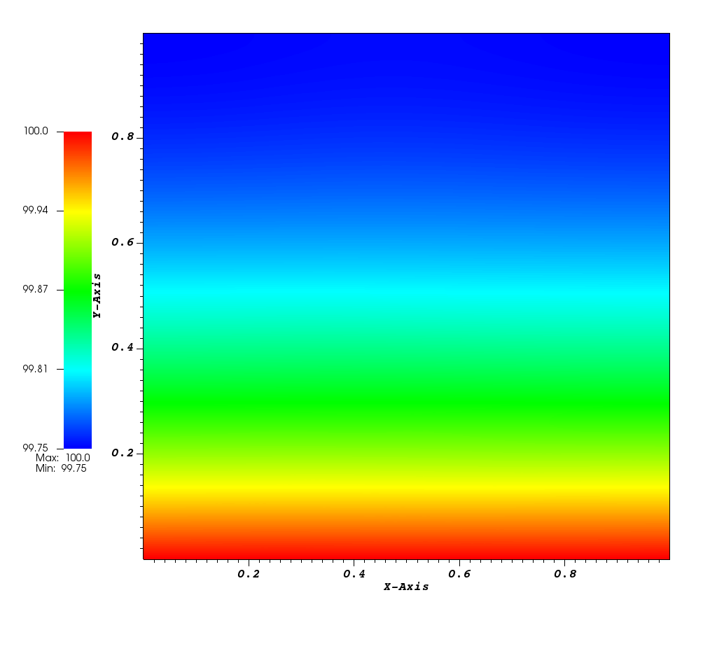
(a) CASE 1

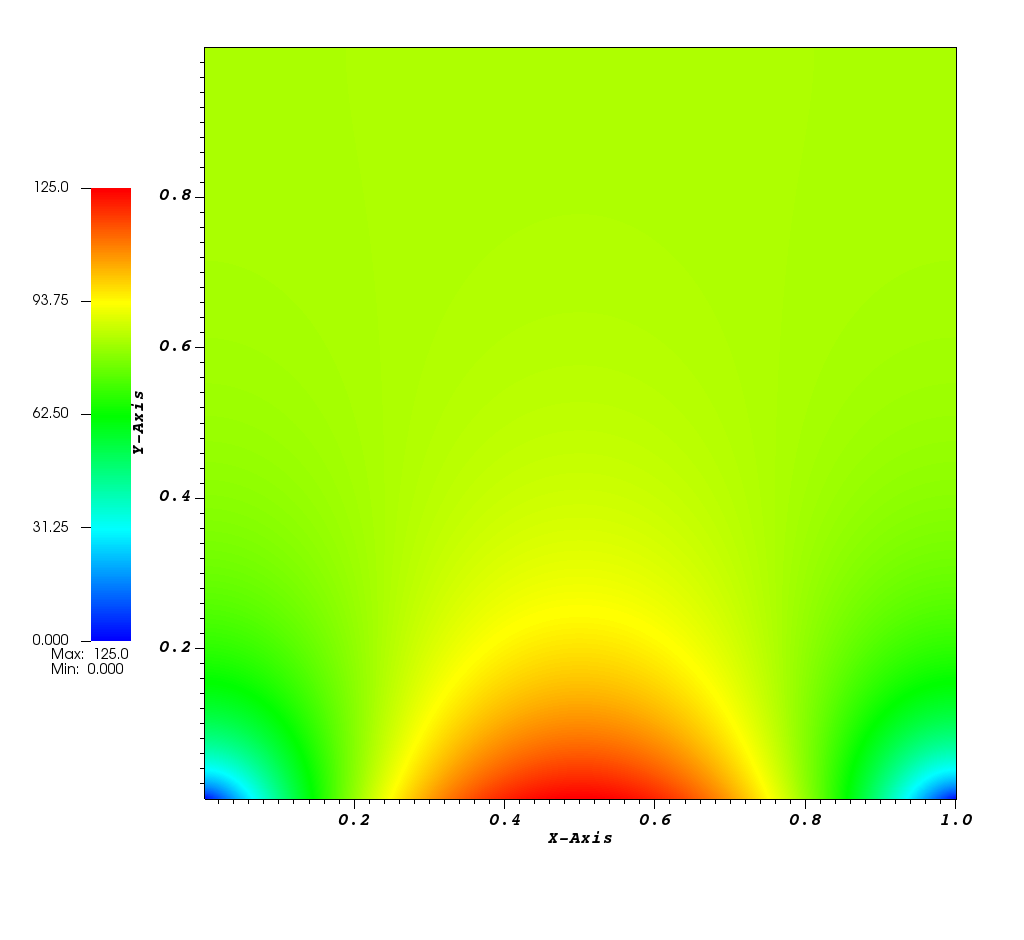
(b) CASE 2

Figure 3: (Example 1) Temperature distribution for CASE 1 and CASE 2.

Temperature  The temperature distribution in this example with both cases (CASE 1 and 2 in (74)) are shown in Figure 3. Since CASE $1$ (Figure 3 (a)) has a constant temperature value on the boundary $\Gamma_{1}$, i.e., $\theta_{1}(x)=100,\;0\leq x\leq 1$, and a uniform heat source $g=-10$ working as a sink over the domain, therefore we can see a uniform distribution of temperature in each layer from the bottom. For the same value of heat source, CASE $2$ (Figure 3 (b)) has a quadratic function $\theta_{2}(x)=500x\,(1-x),\;0\leq x\leq 1$, on the bottom boundary $\Gamma_{1}$, resulting in the non-uniform temperature distribution at each height near the bottom. With these known solutions of temperature effecting on the momentum, next we present the numerical solutions for the displacement variable in the material body.

(CASE $1$) Linear  By taking $\beta=0$ in (70b), we obtain the solution to the linear model. Figure 4 depicts the displacement components, (a) $\bm{u}_{x}$ and (b) $\bm{u}_{y}$ in the whole domain. Figure 5 presents the axial stress ($\bm{T}_{yy}$) and the axial strain ($\bm{\epsilon}_{yy}$) plots, respectively.

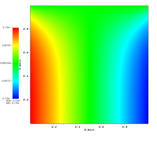
(a) $\bm{u}_{x}$

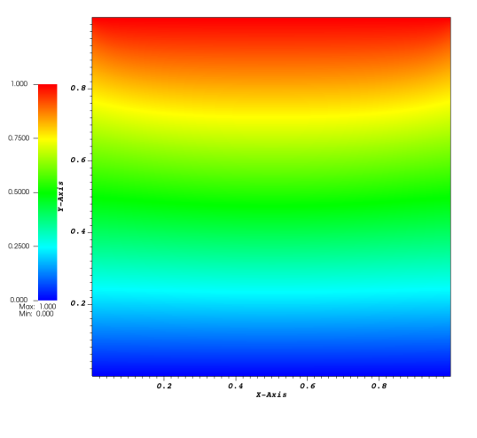
(b) $\bm{u}_{y}$

Figure 4: (Example 1 with CASE 1) Displacement for the Linear: (a) x-displacement and (b) y-displacement.

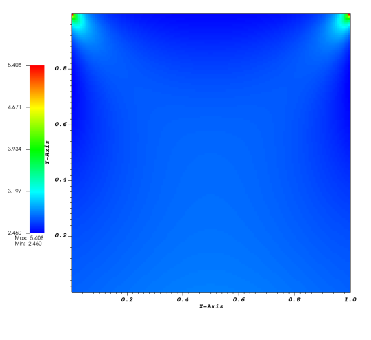
(a) $\bm{T}_{yy}$

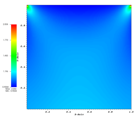
(b) $\bm{\epsilon}_{yy}$

Figure 5: (Example 1 with CASE 1) Stress and Strain for the Linear: (a) axial stress and (b) axial strain.

(CASE $1$) Nonlinear  Here, we solve the nonlinear model with CASE $1$ type temperature boundary condition. Figure 6 depicts the displacement components $\bm{u}_{x}$ and $\bm{u}_{y}$ and the axial stress ($\bm{T}_{yy}$) and the axial strain ($\bm{\epsilon}_{yy}$) components are presented in Figure 7. Note that for displacement, the overall pattern of the distributions and values (e.g., the maximum and the minimum values in $\bm{u}_{x}$) is almost the same as the one for (CASE $1$) Linear (Figure 4). In case for the axial stress ($\bm{T}_{yy}$) and the axial strain ($\bm{\epsilon}_{yy}$) for the nonlinear model, the patterns are similar to the linear model, but the the maximum and the minimum in the axial strain is much lower for the nonlinear model as expected. Compared to the axial strain, we see that the difference in axial stress between the two models is not much intense.

(a) $\bm{u}_{x}$

(b) $\bm{u}_{y}$

Figure 6: (Example 1 with CASE 1) Displacement for the Nonlinear: (a) x-displacement and (b) y-displacement.

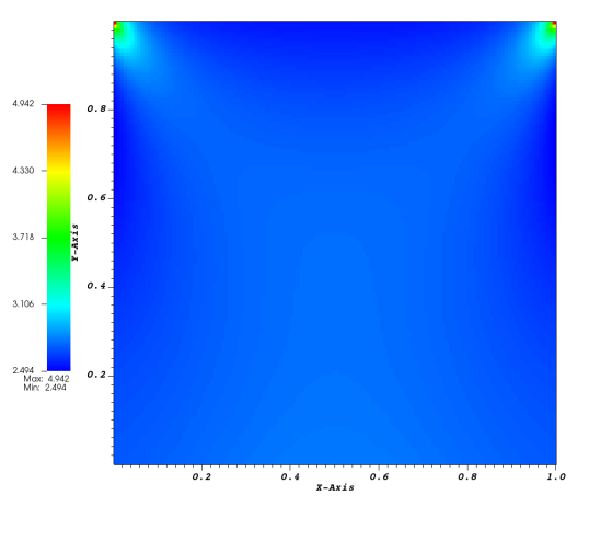
(a) $\bm{T}_{yy}$

(b) $\bm{\epsilon}_{yy}$

Figure 7: (Example 1 with CASE 1) Stress and Strain for the Nonlinear: (a) axial stress and (b) axial strain.

(CASE $2$) Linear Next, we present the computational results for the second type of temperature boundary condition (CASE 2) with the linear model. Figure 8 shows the displacement field in the entire body. We see that the displacement component $\bm{u}_{y}$ has a parabolic type distribution on the bottom face due to the applied temperature boundary condition on $\Gamma_{1}$. Corresponding distribution of axial stress-strain in $y$-direction is shown in Figure 9.

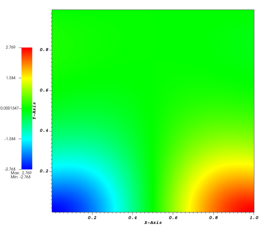
(a) $\bm{u}_{x}$

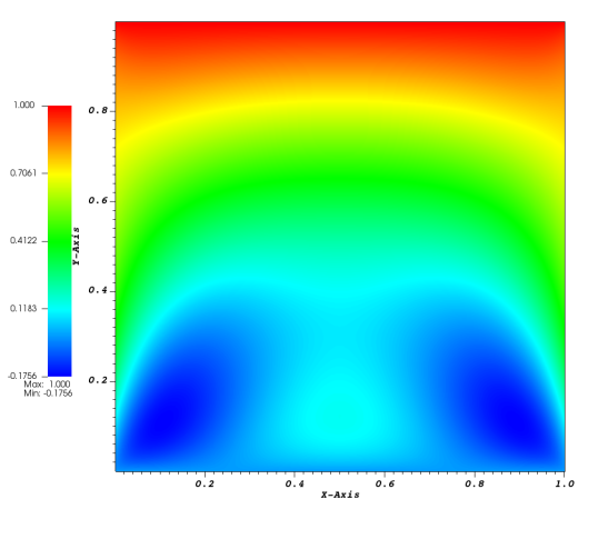
(b) $\bm{u}_{y}$

Figure 8: (Example 1 with CASE 2) Displacement for the Linear: (a) x-displacement and (b) y-displacement

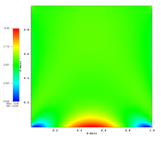
(a) $\bm{T}_{yy}$

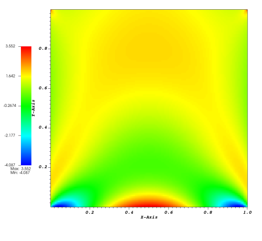
(b) $\bm{\epsilon}_{yy}$

Figure 9: (Example 1 with CASE 2) Stress and Strain for the Linear: (a) axial stress and (b) axial strain.

(CASE $2$) Nonlinear We explore the effect of the quadratic temperature boundary condition on the response of the material body characterized by the nonlinear relation between stress and strain. Figure 10 represents the displacement field in this case. Unlike CASE 1, the parabolic distribution of bottom temperature in CASE 2 within the nonlinear model has noticeble effects on the mechanics and brings different maximum and minimum values between the models for each displacement component (Figure 10). Similarly, distinct patterns are found in axial stress and strain distributions (Figure 11). For the linear model, the maximum and minimum values for both stress and strain aggregate densely closer to the bottom boundary $\Gamma_{1}$ where the non-uniform (or closer to a point/region) heat source is located. Meanwhile, the nonlinear model has more distributed pattern over the domain with smaller values, especially for the strain. Similar type of effects of distribution patterns for the linear and the nonlinear models can be found in Example 2 in the following where the tip area of slit works as another boundary related to the stress. Compared to CASE 1, overall we see that CASE 2 has more different distributions of the field variables between the linear and the nonlinear models.

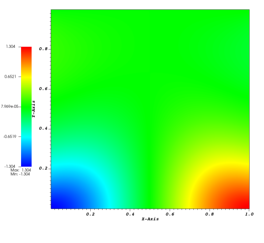
(a) $\bm{u}_{x}$

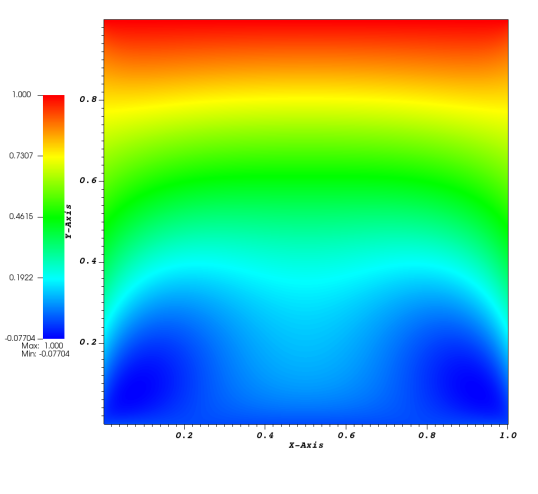
(b) $\bm{u}_{y}$

Figure 10: (Example 1 with CASE 2) Displacement for the Nonlinear: (a) x-displacement and (b) y-displacement.

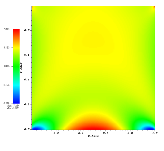
(a) $\bm{T}_{yy}$

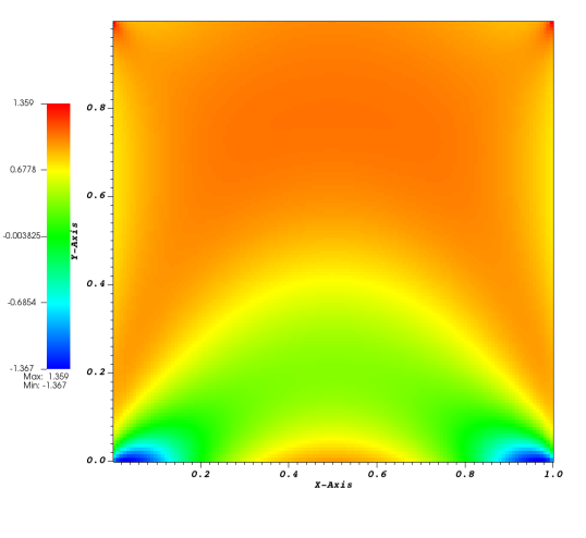
(b) $\bm{\epsilon}_{yy}$

Figure 11: (Example 1 with CASE 2) Stress and Strain for the Nonlinear: (a) axial stress and (b) axial strain.

4.3.2 Example $2$: Domain with a slit

In this example, we have considered has a computational domain with a “slit” as shown in Figure 2. The slit is expressed with two individual vertices at the same coordinate of $(1,0.5)$ on the right boundary $\Gamma_{2}$, resulting in a “crack-opening” deformation on $\Gamma_{C}$. A zero traction boundary condition is imposed on the upper and lower faces of the slit. All other boundary conditions for both variables on all other remaining parts of the boundary are the same as the ones used in Example 1 (as given in (73)-(74)). We also consider the two different temperature boundary conditions given in (74).

Temperature  Figure 12 shows two cases of temperature distribution in this example with two different temperature boundary conditions. Be reminded that CASE 1 has constant temperature boundary condition on the boundary $\Gamma_{1}$. Compared to Example 1 with CASE 1 (Figure 3 (a)), Example 2 with CASE 1 has the temperature distribution less uniform due to the slit at the center of the half right region. Note that we have the homogeneous Neumann boundary condition for temperature on the slit as (76). For CASE 2, quite similar type of the parabolic shape for heat distribution from the bottom face can be seen as Example 1 with CASE 2 (Figure 3 (b)).

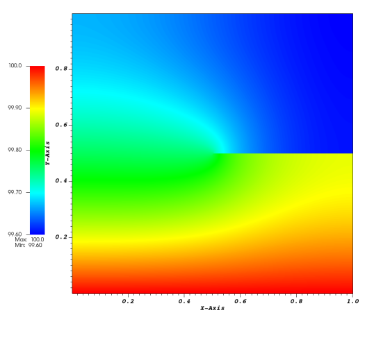
(a) CASE 1

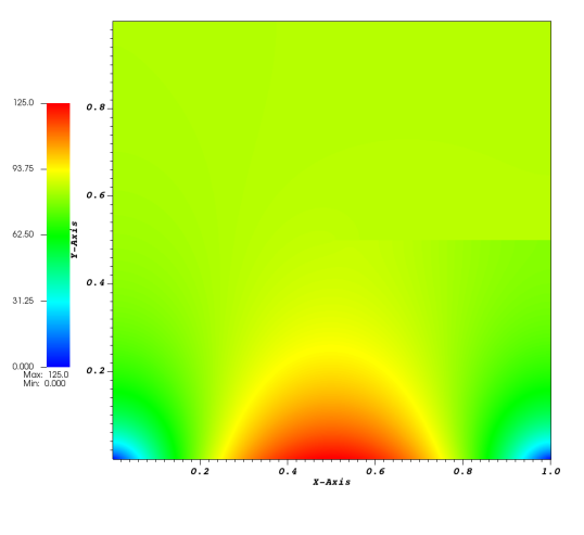
(b) CASE 2

Figure 12: (Example 2) Temperature distribution for CASE 1 and CASE 2.

After unveiling the temperature solution, next we present the numerical results for the displacements for both cases of temperature boundary condition on the bottom boundary as Example 1. The ultimate goal of this research is to report some information about the nature of the solution near the crack-tip when the body is under a combination of thermo-mechanical loading. The numerical results will present a remarkable distinction in the crack-tip stress-strain solutions for the nonlinear strain-limiting and the linearized elasticity models.
(CASE $1$) Linear In this case, a uniform and constant temperature boundary condition is applied on the bottom boundary and the classical constitutive relation for linearized elasticity is used to model the behavior of the bulk material. Likewise, we first present the displacements plot ($\bm{u}_{x}$ and $\bm{u}_{y}$ depicted in Figure 13) followed by the axial stress-strain distribution plots ($\bm{T}_{yy}$ and $\bm{\epsilon}_{yy}$ depicted in Figure 14). Known as the classical square-root order singularity, we can see that stress-strain values in the vicinity of the tip are large.

(a) $\bm{u}_{x}$

(b) $\bm{u}_{y}$

Figure 13: (Example 2 with CASE 1) Displacement for the Linear: (a) x-displacement and (b) y-displacement.

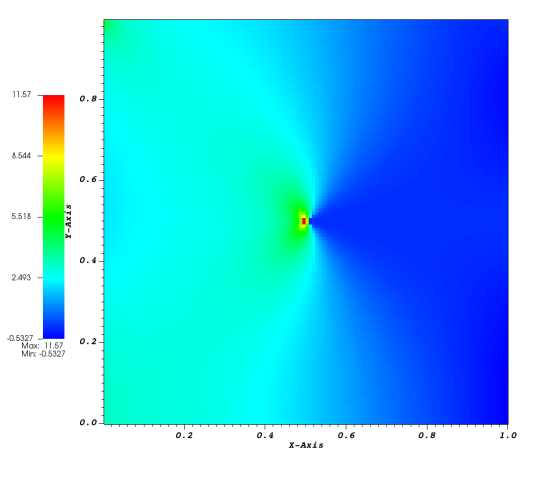
(a) $\bm{T}_{yy}$

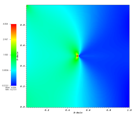
(b) $\bm{\epsilon}_{yy}$

Figure 14: (Example 2 with CASE 1) Stress and Strain for the Linear: (a) axial stress and (b) axial strain.

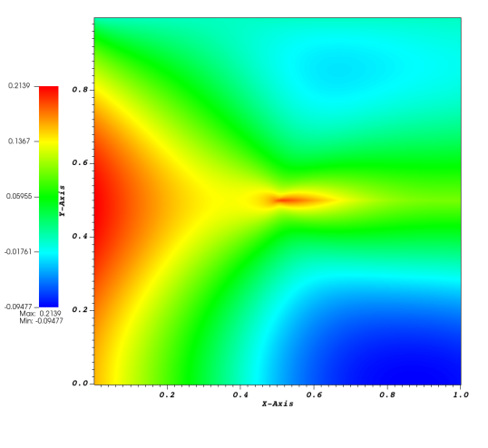
(a) $\bm{u}_{x}$

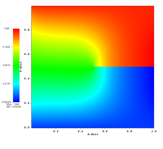
(b) $\bm{u}_{y}$

Figure 15: (Example 2 with CASE 1) Displacement for the Nonlinear: (a) x-displacement field and (b) y-displacement.

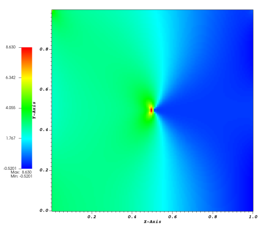
(a) $\bm{T}_{yy}$

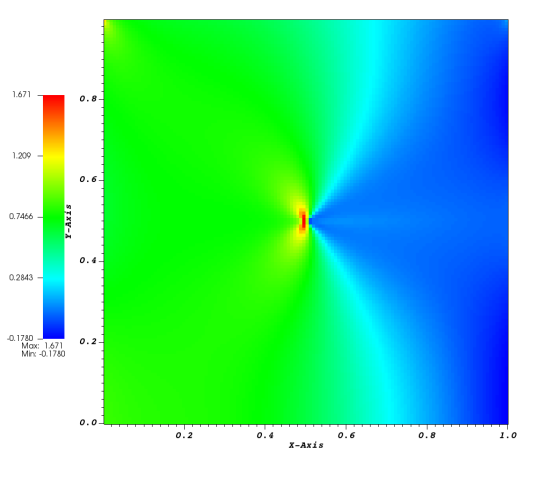
(b) $\bm{\epsilon}_{yy}$

Figure 16: (Example 2 with CASE 1) Stress and Strain for the Nonlinear: (a) axial stress and (b) axial strain.

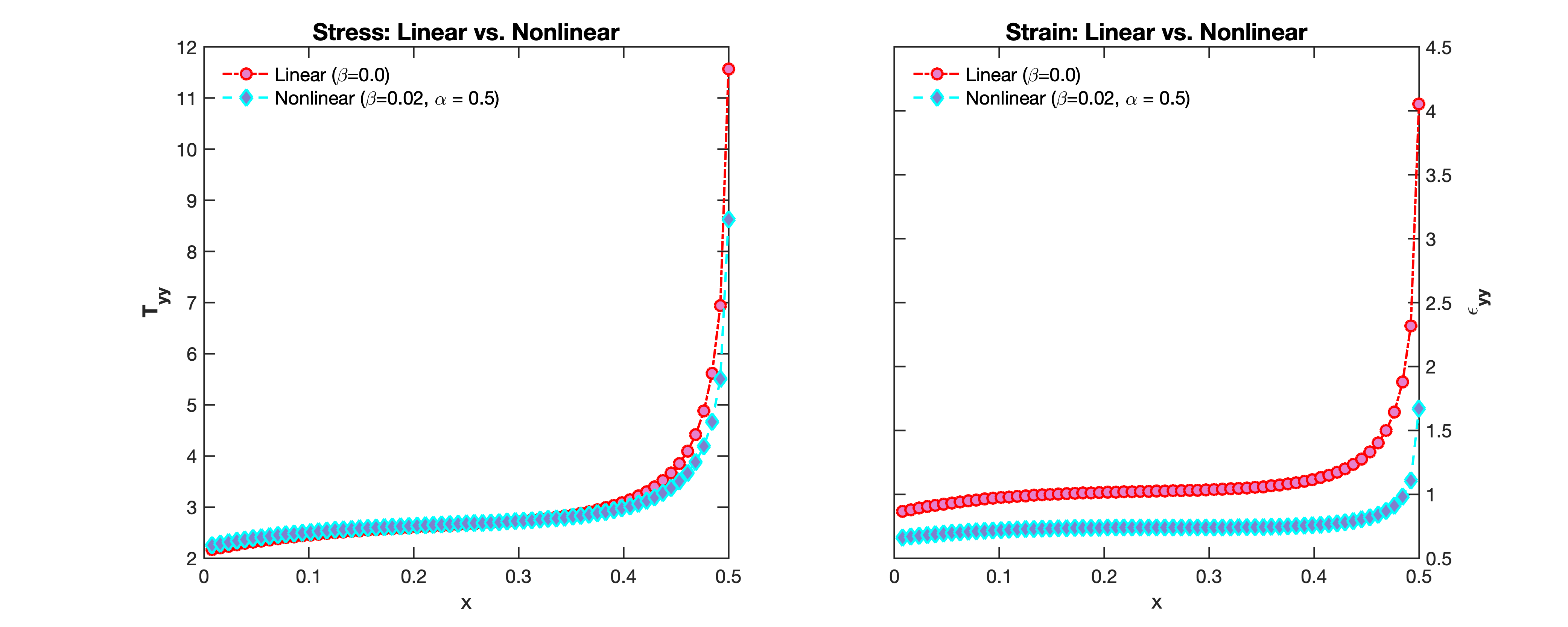
Figure 17: (Example 2 with CASE 1) Linear vs. Nonlinear: stress $\bm{T}_{yy}$ (left) and strain $\bm{\epsilon}_{yy}$ (right) on the reference line.

(CASE $1$) Nonlinear Here, we solve the nonlinear boundary value problem under the constant temperature condition at the bottom. Figure 15 depicts the displacement field $(\bm{u}_{x},\bm{u}_{y})$ and Figure 16 represents the distribution of axial stress and strain components for CASE 1 in Example 2. As similar to Example 1 with CASE 1, the nonlinear model for Example 2 with CASE 1 shows not much difference in its displacement pattern and values from those of the linear model (See Figure 13 and Figure 15.) Likewise for the axial stress, we can clearly see that the distribution seems similar to the linear model especially when approaching the crack tip. Figure 17 shows for the axial stress (left) and the axial strain (right) of the two models on the reference line approaching the tip. For strains, we can see much smaller values along the radial line leading up to the crack-tip, as expected from the nonlinear strain-limiting model. Also note that compared to Figure 14 (b), Figure 16 (b) has a relatively sharper change in color for the legend (e.g., see the cyan-colored line in between the blue and the green) over the domain and in the vicinity of the tip, implying that the the contour lines for the strain near the tip along with the shape of crack for the strain-limiting is much different from the linear model (35).
(CASE $2$) Linear In this last example with the parabolic type of Dirichlet boundary condition for the temperature, we also consider the linear problem first. Figure 18 depicts the displacement fields of $\bm{u}_{x}$ and $\bm{u}_{y}$, respectively. Figure 19 depicts the axial stress and strain fields in the entire material body. It is clear from the stress-strain plots that the values of stress have the corresponding maximum “at the tip”, and strain values are “comparable” with the stress concentration in the neighborhood of the crack-tip. Also note that the next group of large values appear near the bottom boundary $\Gamma_{1}$ due to the parabolic distribution of temperature, which is similar as shown in Example 1 with CASE $2$ (Figure 9).

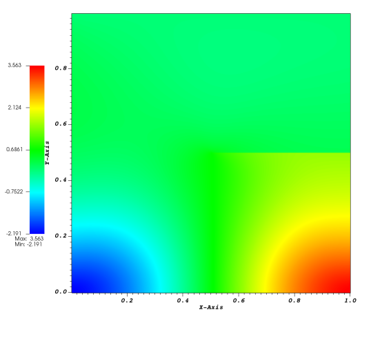
(a) $\bm{u}_{x}$

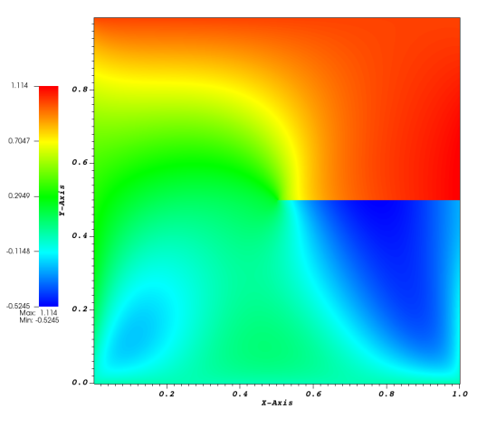
(b) $\bm{u}_{y}$

Figure 18: (Example 2 with CASE 2) Displacement for the Linear: (a) x-displacement and (b) y-displacement.

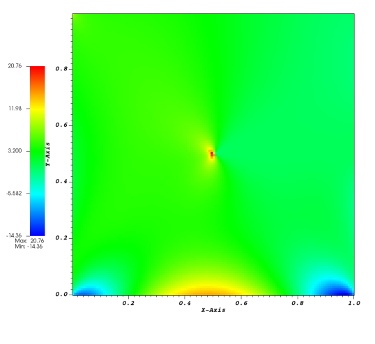
(a) $\bm{T}_{yy}$

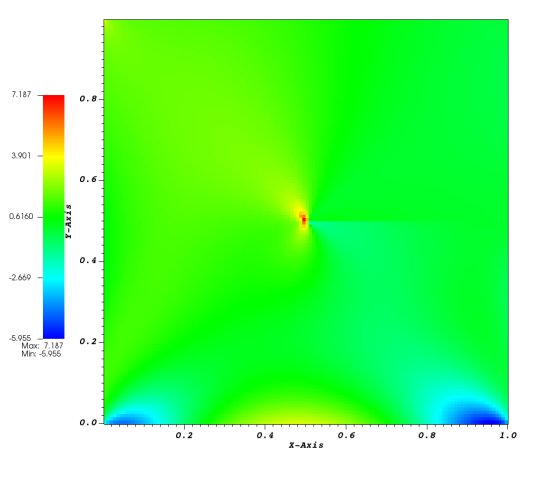
(b) $\bm{\epsilon}_{yy}$

Figure 19: (Example 2 with CASE 2) Stress and Strain for the Linear: (a) axial stress and (b) axial strain.

(CASE $2$) Nonlinear Lastly, we study the nonlinear strain-limiting model with the boundary value problem of the parabolic temperature boundary condition. Figure 20 depicts the displacement field and Figure 21 delineates the stress-strain for the nonlinear model in the whole material body. The differences in their values for displacement, stress and strain between the linear and the nonlinear models get larger for CASE $2$ than the corresponding differences for CASE $1$. Figure 21 (a) clearly characterizes the concentration of the stress in the neighborhood of the crack-tip, whereas Figure 21 (b) represents the bounded strain values which is more distributed over the domain compared to the one for the linear model (Figure 19 (b)). Also from its maximum and minimum values, it can be inferred that the growth of strain is not in the same order as the one for stress but limited. The contrast are clearly shown in Figure 22 depicting the axial stress (left) and the axial strain (right) on the reference line approaching the tip with the two models. We confirm that the growth rate at which stresses are increasing near the crack-tip is much larger than than rate at which the strain does, and there is a clear distinction of the strain behavior between the two models studied in this paper. The stress growth in the neighborhood suggests that the crack-tip is a singular energy sink, therefore one can make use of the local growth criterion to study the crack evolution within the framework of strain-limiting model proposed in this paper. Likewise as seen in Example 1, CASE 2 has more differences between the linear and the nonlinear models than CASE 1 (See Figure 17 and Figure 22).

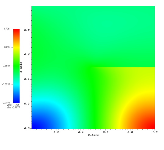
(a) $\bm{u}_{x}$

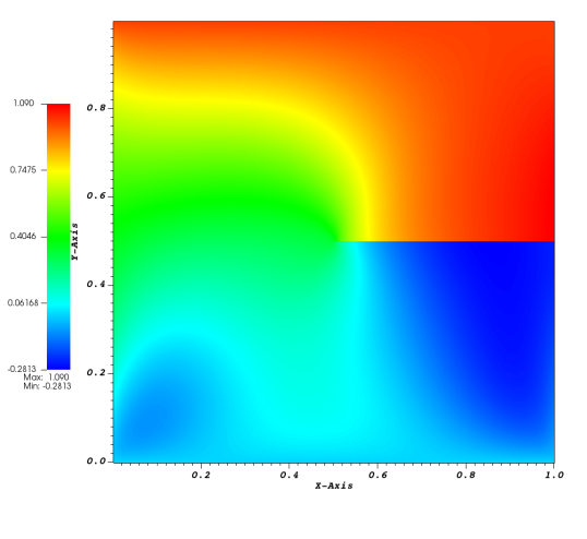
(b) $\bm{u}_{y}$

Figure 20: (Example 2 with CASE 2) Displacement for the Nonlinear: (a) x-displacement and (b) y-displacement.

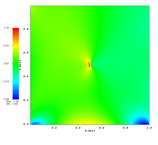
(a) $\bm{T}_{yy}$

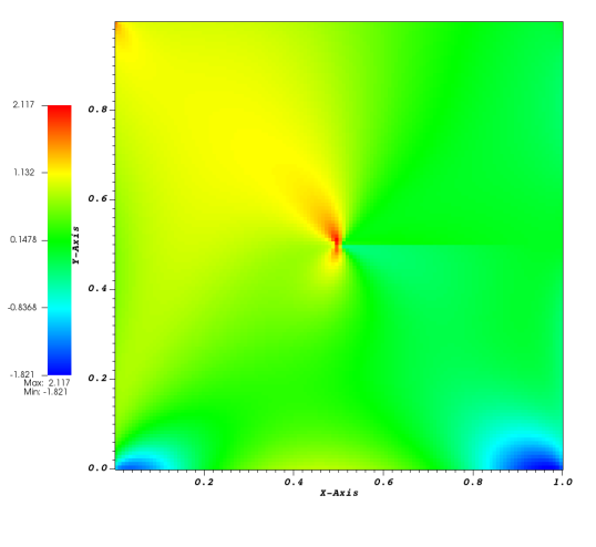
(b) $\bm{\epsilon}_{yy}$

Figure 21: (Example 2 with CASE 2) Stress and Strain for the Nonlinear: (a) axial stress and (b) axial strain.

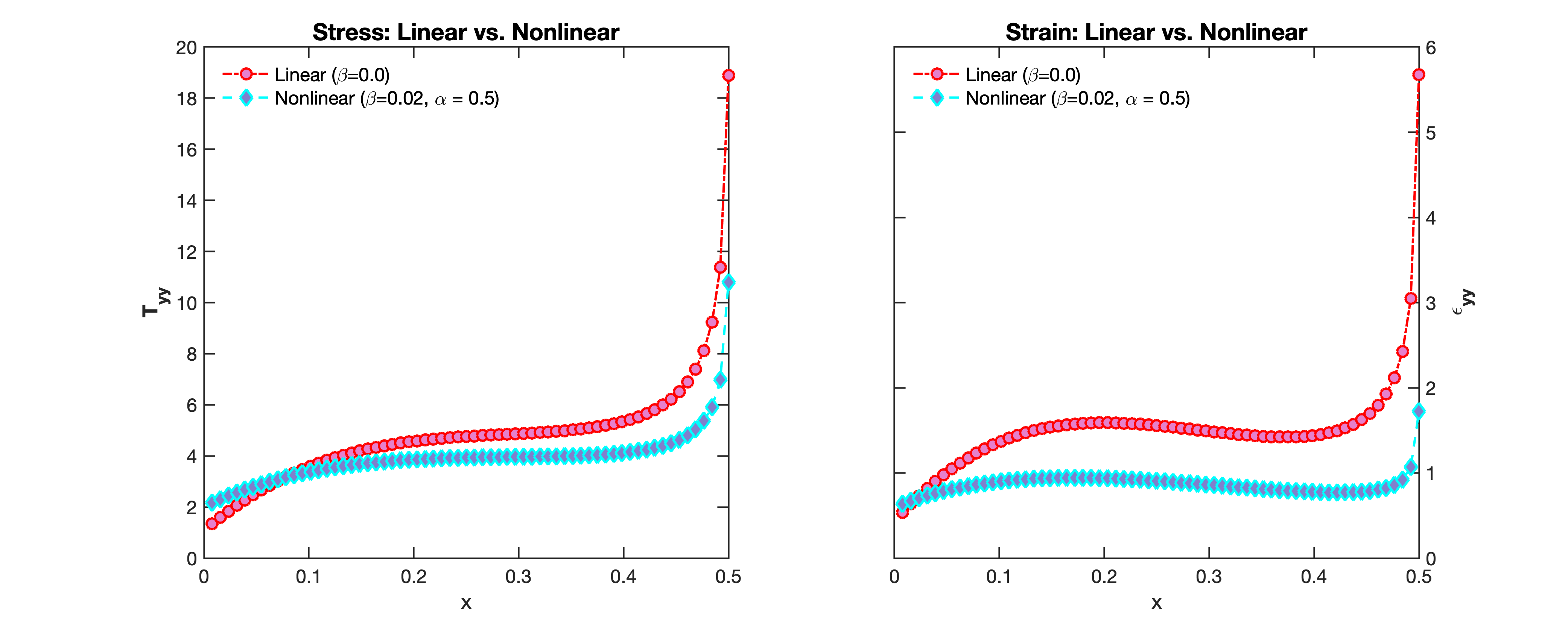
Figure 22: (Example 2 with CASE 2) Linear vs. Nonlinear: stress $\bm{T}_{yy}$ (left) and strain $\bm{\epsilon}_{yy}$ (right) on the reference line.

5 Conclusion

In the present paper, we have studied a finite element discretization of some boundary value problems formulated within a relatively new class of strain-limiting nonlinear constitutive relations. The present study is an extension of constitutive theory developed in (17) to the generalized thermoelasticity. We formulate a well-posed mathematical model to describe the response state of the elastic body under thermo-mechanical loading. Since the model consists of a nonlinear relationship between stress and strain, numerical discretization is not straightforward. A key approach in its formulation is the linearization using Newton’s method, therefore it require us to solve one elliptic boundary value problem at each Newton’s step. Numerical experiments provide a solid evidence in support for the efficacy of the proposed model. We observe the crack-tip stress concentration, similar to the classical model, but the growth of strain does not behave similarly to that of stress but as expected with a slower order for growth near the tip. As a part of the future work, an immediate next step can include extending the model studied in this paper for the quasi-static evolution of network of cracks under thermo-mechanical loading. Furthermore, the formulation studied in this article can also be extended to study a reliable constitutive relation for the heat such as the wave propagation without energy dissipation for the Fourier’s law.

References

- Brown et al. (2008) Brown, D., et al. Applied Mathematics at the U.S. Department of Energy: Past, Present, and a View to the Future. 2008.
- Cattaneo (1958) Cattaneo, C.. A form of heat-conduction equations which eliminates the paradox of instantaneous propagation. Comptes Rendus 1958;247:431.
- Vernotte (1958) Vernotte, P.. Les paradoxes de la theorie continue de l’equation de la chaleur. Compt Rendu 1958;246:3154–3155.
- Marín (2011) Marín, E.. Does fourier’s law of heat conduction contradict the theory of relativity? Latin-American Journal of Physics Education 2011;5(2):13.
- Chester (1963) Chester, M.. Second sound in solids. Physical Review 1963;131(5):2013.
- Lord and Shulman (1967) Lord, H.W., Shulman, Y.. A generalized dynamical theory of thermoelasticity. Journal of the Mechanics and Physics of Solids 1967;15(5):299–309.
- Chandrasekharaiah (1986) Chandrasekharaiah, D.. Thermoelasticity with second sound: a review. ASME Appl Mech Rev March 1986;39(3):355–376.
- Chandrasekharaiah (1998) Chandrasekharaiah, D.. Hyperbolic thermoelasticity: a review of recent literature 1998;.
- Agrawal (2016) Agrawal, A.. Higher-order continuum equation based heat conduction law. INAE Letters 2016;1(2):35–39.
- Whitaker (2013) Whitaker, S.. Fundamental principles of heat transfer. Elsevier; 2013.
- Broberg (1999) Broberg, K.. Cracks and fracture. Academic Press; 1999.
- Anderson (2017) Anderson, T.L.. Fracture mechanics: fundamentals and applications. CRC press; 2017.
- Barenblatt (1962) Barenblatt, G.I.. The mathematical theory of equilibrium cracks in brittle fracture. In: Advances in applied mechanics; vol. 7. Elsevier; 1962, p. 55–129.
- Gurtin and Murdoch (1975) Gurtin, M.E., Murdoch, A.I.. A continuum theory of elastic material surfaces. Archive for Rational Mechanics and Analysis 1975;57(4):291–323.
- Sendova and Walton (2010) Sendova, T., Walton, J.R.. A new approach to the modeling and analysis of fracture through extension of continuum mechanics to the nanoscale. Mathematics and Mechanics of Solids 2010;15(3):368–413.
- Ferguson et al. (2015) Ferguson, L.A., Muddamallappa, M., Walton, J.R.. Numerical simulation of mode-iii fracture incorporating interfacial mechanics. International Journal of Fracture 2015;192(1):47–56.
- Rajagopal (2007) Rajagopal, K.. The elasticity of elasticity. Zeitschrift für Angewandte Mathematik und Physik (ZAMP) 2007;58(2):309–317.
- Rajagopal and Srinivasa (2007) Rajagopal, K., Srinivasa, A.. On the response of non-dissipative solids. In: Proceedings of the Royal Society of London A: Mathematical, Physical and Engineering Sciences; vol. 463. The Royal Society; 2007, p. 357–367.
- Rajagopal and Saccomandi (2016) Rajagopal, K., Saccomandi, G.. A novel approach to the description of constitutive relations. Frontiers in Materials 2016;3:36.
- Bustamante and Rajagopal (2020) Bustamante, R., Rajagopal, K.. A review of implicit constitutive theories to describe the response of elastic bodies. In: Constitutive Modelling of Solid Continua. Springer; 2020, p. 187–230.
- Rajagopal (2003) Rajagopal, K.. On implicit constitutive theories. Applications of Mathematics 2003;48(4):279–319.
- Rajagopal and Walton (2011) Rajagopal, K., Walton, J.. Modeling fracture in the context of a strain-limiting theory of elasticity: a single anti-plane shear crack. International journal of fracture 2011;169(1):39–48.
- Gou et al. (2015) Gou, K., Mallikarjunaiah, S., Rajagopal, K., Walton, J.. Modeling fracture in the context of a strain-limiting theory of elasticity: A single plane-strain crack. International Journal of Engineering Science 2015;88:73–82.
- Mallikarjunaiah and Walton (2015) Mallikarjunaiah, S., Walton, J.. On the direct numerical simulation of plane-strain fracture in a class of strain-limiting anisotropic elastic bodies. International Journal of Fracture 2015;192(2):217–232.
- Kulvait et al. (2013) Kulvait, V., Málek, J., Rajagopal, K.. Anti-plane stress state of a plate with a V-notch for a new class of elastic solids. International Journal of Fracture 2013;179(1-2):59–73.
- Kulvait et al. (2019) Kulvait, V., Málek, J., Rajagopal, K.. The state of stress and strain adjacent to notches in a new class of nonlinear elastic bodies. Journal of Elasticity 2019;135(1-2):375–397.
- Bustamante and Rajagopal (2010) Bustamante, R., Rajagopal, K.. A note on plane strain and plane stress problems for a new class of elastic bodies. Mathematics and Mechanics of Solids 2010;15(2):229–238.
- Bustamante and Rajagopal (2011) Bustamante, R., Rajagopal, K.. Solutions of some simple boundary value problems within the context of a new class of elastic materials. International Journal of Non-Linear Mechanics 2011;46(2):376–386.
- Bustamante and Rajagopal (2015) Bustamante, R., Rajagopal, K.. Implicit constitutive relations for nonlinear magnetoelastic bodies. Proceedings of the Royal Society A: Mathematical, Physical and Engineering Sciences 2015;471(2175):20140959.
- Ortiz et al. (2012) Ortiz, A., Bustamante, R., Rajagopal, K.. A numerical study of a plate with a hole for a new class of elastic bodies. Acta Mechanica 2012;223(9):1971–1981.
- Bustamante and Rajagopal (2018) Bustamante, R., Rajagopal, K.. A nonlinear model for describing the mechanical behaviour of rock. Acta Mechanica 2018;229(1):251–272.
- Fu et al. (2019) Fu, S., Chung, E., Mai, T.. Generalized multiscale finite element method for a strain-limiting nonlinear elasticity model. Journal of Computational and Applied Mathematics 2019;359:153–165.
- Fu et al. (2020) Fu, S., Chung, E., Mai, T.. Constraint energy minimizing generalized multiscale finite element method for nonlinear poroelasticity and elasticity. Journal of Computational Physics 2020;417:109569.
- Ortiz-Bernardin et al. (2014) Ortiz-Bernardin, A., Bustamante, R., Rajagopal, K.. A numerical study of elastic bodies that are described by constitutive equations that exhibit limited strains. International Journal of Solids and Structures 2014;51(3-4):875–885.
- Yoon and Mallikarjunaiah (2021) Yoon, H., Mallikarjunaiah, S.. A finite element discretization of some boundary value problems for nonlinear strain-limiting elastic bodies. Mathematics and Mechanics of Solids 2021;:In pressURL: https://doi.org/10.1177/10812865211020789.
- Lee et al. (2020) Lee, S., Yoon, H.C., Mallikarjunaiah, S.. Nonlinear strain-limiting elasticity for fracture propagation with phase-field approach. arXiv preprint arXiv:200711101 2020;.
- Yoon et al. (2021) Yoon, H.C., Lee, S., Mallikarjunaiah, S.. Quasi-static anti-plane shear crack propagation in nonlinear strain-limiting elastic solids using phase-field approach. International Journal of Fracture 2021;227(2):153–172.
- Bourdin et al. (2000) Bourdin, B., Francfort, G.A., Marigo, J.J.. Numerical experiments in revisited brittle fracture. Journal of the Mechanics and Physics of Solids 2000;48(4):797–826.
- Ciarlet (2002) Ciarlet, P.G.. The finite element method for elliptic problems. SIAM; 2002.
- Evans (1998) Evans, L.C.. Partial differential equations. Graduate studies in mathematics 1998;19(2).
- Rajagopal (2011a) Rajagopal, K.. Non-linear elastic bodies exhibiting limiting small strain. Mathematics and Mechanics of Solids 2011a;16(1):122–139.
- Rajagopal (2011b) Rajagopal, K.. Conspectus of concepts of elasticity. Mathematics and Mechanics of Solids 2011b;16(5):536–562.
- Rajagopal (2014) Rajagopal, K.. On the nonlinear elastic response of bodies in the small strain range. Acta Mechanica 2014;225(6):1545–1553.
- Mallikarjunaiah (2015) Mallikarjunaiah, S.. On two theories for brittle fracture: Modeling and direct numerical simulations. Ph.D. thesis; Texas A&M University; 2015.
- Itoui et al. (2018) Itoui, H., Kovtunenko, V., Rajagopal, K.. On the states of stress and strain adjacent to a crack in a strain-limiting viscoelastic body. Mathematics and Mechanics of Solids 2018;23(3):433–444.
- Bulíček et al. (2014) Bulíček, M., Málek, J., Rajagopal, K., Süli, E.. On elastic solids with limiting small strain: modelling and analysis. EMS Surveys in Mathematical Sciences 2014;1(2):283–332.
- Kannan et al. (2014) Kannan, K., Rajagopal, K., Saccomandi, G.. Unsteady motions of a new class of elastic solids. Wave Motion 2014;51(5):833–843.
- Kambapalli et al. (2014) Kambapalli, M., Kannan, K., Rajagopal, K.. Circumferential stress waves in a non-linear cylindrical annulus in a new class of elastic materials. The Quarterly Journal of Mechanics and Applied Mathematics 2014;67(2):193–203.
- Bridges and Rajagopal (2015) Bridges, C., Rajagopal, K.. Implicit constitutive models with a thermodynamic basis: a study of stress concentration. Zeitschrift für angewandte Mathematik und Physik 2015;66(1):191–208.
- Bustamante and Rajagopal (2017) Bustamante, R., Rajagopal, K.. Implicit equations for thermoelastic bodies. International Journal of Non-Linear Mechanics 2017;92:144–152.
- Callen (1998) Callen, H.B.. Thermodynamics and an introduction to thermostatistics. 1998.
- Mai and Walton (2015a) Mai, T., Walton, J.. On strong ellipticity for implicit and strain-limiting theories of elasticity. Mathematics and Mechanics of Solids 2015a;20(2):121–139.
- Mai and Walton (2015b) Mai, T., Walton, J.R.. On monotonicity for strain-limiting theories of elasticity. Journal of Elasticity 2015b;120(1):39–65.
- Bulíček et al. (2015a) Bulíček, M., Málek, J., Rajagopal, K., Walton, J.R.. Existence of solutions for the anti-plane stress for a new class of “strain-limiting” elastic bodies. Calculus of Variations and Partial Differential Equations 2015a;54(2):2115–2147.
- Beck et al. (2017) Beck, L., Bulíček, M., Málek, J., Süli, E.. On the existence of integrable solutions to nonlinear elliptic systems and variational problems with linear growth. Archive for Rational Mechanics and Analysis 2017;225(2):717–769.
- Bulíček et al. (2015b) Bulíček, M., Málek, J., Süli, E.. Analysis and approximation of a strain-limiting nonlinear elastic model. Mathematics and Mechanics of Solids 2015b;20(1):92–118.
- Bonito et al. (2020) Bonito, A., Girault, V., Süli, E.. Finite element approximation of a strain-limiting elastic model. IMA Journal of Numerical Analysis 2020;40(1):29–86.
- Saad (2003) Saad, Y.. Iterative methods for sparse linear systems. SIAM; 2003.
- Eisenstat (1981) Eisenstat, S.C.. Efficient implementation of a class of preconditioned conjugate gradient methods. SIAM Journal on Scientific and Statistical Computing 1981;2(1):1–4.
- Alzetta et al. (2018) Alzetta, G., Arndt, D., Bangerth, W., Boddu, V., Brands, B., Davydov, D., et al. The deal. II library, version 9.0. Journal of Numerical Mathematics 2018;26(4):173–183.