Atlas Based Representation and Metric Learning on Manifolds

Abstract

We explore the use of a topological manifold, represented as a collection of charts, as the target space of neural network based representation learning tasks. This is achieved by a simple adjustment to the output of an encoder’s network architecture plus the addition of a maximal mean discrepancy (MMD) based loss function for regularization. Most algorithms in representation and metric learning are easily adaptable to our framework and we demonstrate its effectiveness by adjusting SimCLR (for representation learning) and standard triplet loss training (for metric learning) to have manifold encoding spaces. Our experiments show that we obtain a substantial performance boost over the baseline for low dimensional encodings. In the case of triplet training, we also find, independent of the manifold setup, that the MMD loss alone (i.e. keeping a flat, euclidean target space but using an MMD loss to regularize it) increases performance over the baseline in the typical, high-dimensional Euclidean target spaces. Code for reproducing experiments is provided at https://github.com/ekorman/neurve.

1 Introduction

Representation learning algorithms typically produce encodings into a Euclidean space. However, if the manifold hypothesis (the assumption that the data is well-approximated by a manifold) is taken seriously then a Euclidean target space is unnecessarily big for encoding this manifold: by the Whitney embedding theorem, to embed an $n$-dimensional manifold into a Euclidean space one may need up to $2n$ dimensions for the ambient space. The situation is even worse if the embedding is required to preserve distances (which is obviously important for metric learning), as the Nash embedding theorem shows that in this case the dimension of the ambient space needed is $\mathcal{O}(n^{2})$ Andrews et al. (2002). Additionally, such algorithms seldom regularize the encoding space (i.e. encourage it to look like a prior distribution) to ensure that it is well-behaved.

In this work we develop a framework for using a manifold as a target space of deep representation learning algorithms. Following our prior work (Korman, 2018), which uses manifolds as the latent space of an autoencoder, this is done by having the encoding network output chart embeddings and membership probabilities for an atlas of a manifold. In other words, instead of learning a single encoder $f:\mathcal{X}\to\mathbb{R}^{d}$ (where $\mathcal{X}$ is the input data and $\mathbb{R}^{d}$ is the Euclidean encoding space), our technique learns $n$-such encoders together with a scoring function $q:\mathcal{X}\to[0,1]^{n}$ that determines which encoding output to use for a given input. Figure 1 shows such an example for $\mathcal{X}$ a circle. For matching the distribution of embeddings to a manifold prior, we introduce a maximal mean discrepancy (MMD) (Gretton et al., 2012) loss for manifolds.

$$\operatorname*{argmax}q(x)=\begin{cases}1;&x\in\leavevmode\hbox to5.37pt{\vbox to13.12pt{\pgfpicture\makeatletter\hbox{\hskip 19.19421pt\lower 11.92044pt\hbox to0.0pt{\pgfsys@beginscope\pgfsys@invoke{ }\definecolor{pgfstrokecolor}{rgb}{0,0,0}\pgfsys@color@rgb@stroke{0}{0}{0}\pgfsys@invoke{ }\pgfsys@color@rgb@fill{0}{0}{0}\pgfsys@invoke{ }\pgfsys@setlinewidth{0.4pt}\pgfsys@invoke{ }\nullfont\hbox to0.0pt{\pgfsys@beginscope\pgfsys@invoke{ }{}{{}}{}{{}{}{}{{}}{{{{}{}{}{}}} {{}{}{}{}}}}{} {} {} {} {}{}\pgfsys@beginscope\pgfsys@invoke{ }\color[rgb]{0.88671875,0.2890625,0.19921875}\definecolor[named]{pgfstrokecolor}{rgb}{0.88671875,0.2890625,0.19921875}\pgfsys@color@rgb@stroke{0.88671875}{0.2890625}{0.19921875}\pgfsys@invoke{ }\pgfsys@color@rgb@fill{0.88671875}{0.2890625}{0.19921875}\pgfsys@invoke{ }\definecolor[named]{pgffillcolor}{rgb}{0.88671875,0.2890625,0.19921875}\pgfsys@setlinewidth{0.8pt}\pgfsys@invoke{ }{}\pgfsys@moveto{-14.22638pt}{24.64087pt}\pgfsys@curveto{-17.62851pt}{22.67665pt}{-18.79422pt}{18.32619pt}{-16.83pt}{14.92406pt}\pgfsys@curveto{-16.20569pt}{13.8428pt}{-15.30763pt}{12.94475pt}{-14.22638pt}{12.32043pt}\pgfsys@stroke\pgfsys@invoke{ } \pgfsys@invoke{\lxSVG@closescope }\pgfsys@endscope \pgfsys@invoke{\lxSVG@closescope }\pgfsys@endscope{}{}{}\hss}\pgfsys@discardpath\pgfsys@invoke{\lxSVG@closescope }\pgfsys@endscope\hss}}\lxSVG@closescope\endpgfpicture}}\\ 2;&x\in\leavevmode\hbox to11.47pt{\vbox to7.91pt{\pgfpicture\makeatletter\hbox{\hskip-17.38298pt\lower-0.4pt\hbox to0.0pt{\pgfsys@beginscope\pgfsys@invoke{ }\definecolor{pgfstrokecolor}{rgb}{0,0,0}\pgfsys@color@rgb@stroke{0}{0}{0}\pgfsys@invoke{ }\pgfsys@color@rgb@fill{0}{0}{0}\pgfsys@invoke{ }\pgfsys@setlinewidth{0.4pt}\pgfsys@invoke{ }\nullfont\hbox to0.0pt{\pgfsys@beginscope\pgfsys@invoke{ }{}{{}}{}{{}{}{}{{}}{{{{}{}{}{}}} {{}{}{}{}}}}{} {} {} {} {}{}\pgfsys@beginscope\pgfsys@invoke{ }\color[rgb]{0.203125,0.54296875,0.7421875}\definecolor[named]{pgfstrokecolor}{rgb}{0.203125,0.54296875,0.7421875}\pgfsys@color@rgb@stroke{0.203125}{0.54296875}{0.7421875}\pgfsys@invoke{ }\pgfsys@color@rgb@fill{0.203125}{0.54296875}{0.7421875}\pgfsys@invoke{ }\definecolor[named]{pgffillcolor}{rgb}{0.203125,0.54296875,0.7421875}\pgfsys@setlinewidth{0.8pt}\pgfsys@invoke{ }{}\pgfsys@moveto{28.45276pt}{0.0pt}\pgfsys@curveto{28.45276pt}{3.92854pt}{25.26811pt}{7.11319pt}{21.33957pt}{7.11319pt}\pgfsys@curveto{20.09094pt}{7.11319pt}{18.86423pt}{6.78453pt}{17.78297pt}{6.16022pt}\pgfsys@stroke\pgfsys@invoke{ } \pgfsys@invoke{\lxSVG@closescope }\pgfsys@endscope \pgfsys@invoke{\lxSVG@closescope }\pgfsys@endscope{}{}{}\hss}\pgfsys@discardpath\pgfsys@invoke{\lxSVG@closescope }\pgfsys@endscope\hss}}\lxSVG@closescope\endpgfpicture}}\\ 3;&x\in\leavevmode\hbox to11.47pt{\vbox to8.92pt{\pgfpicture\makeatletter\hbox{\hskip 14.62637pt\lower-27.00508pt\hbox to0.0pt{\pgfsys@beginscope\pgfsys@invoke{ }\definecolor{pgfstrokecolor}{rgb}{0,0,0}\pgfsys@color@rgb@stroke{0}{0}{0}\pgfsys@invoke{ }\pgfsys@color@rgb@fill{0}{0}{0}\pgfsys@invoke{ }\pgfsys@setlinewidth{0.4pt}\pgfsys@invoke{ }\nullfont\hbox to0.0pt{\pgfsys@beginscope\pgfsys@invoke{ }{}{{}}{}{{}{}{}{{}}{{{{}{}{}{}}} {{}{}{}{}}}}{} {} {} {} {}{}\pgfsys@beginscope\pgfsys@invoke{ }\color[rgb]{0.42578125,0.56640625,0.30859375}\definecolor[named]{pgfstrokecolor}{rgb}{0.42578125,0.56640625,0.30859375}\pgfsys@color@rgb@stroke{0.42578125}{0.56640625}{0.30859375}\pgfsys@invoke{ }\pgfsys@color@rgb@fill{0.42578125}{0.56640625}{0.30859375}\pgfsys@invoke{ }\definecolor[named]{pgffillcolor}{rgb}{0.42578125,0.56640625,0.30859375}\pgfsys@setlinewidth{0.8pt}\pgfsys@invoke{ }{}\pgfsys@moveto{-14.22638pt}{-24.64087pt}\pgfsys@curveto{-10.82425pt}{-26.60509pt}{-6.47379pt}{-25.43938pt}{-4.50957pt}{-22.03725pt}\pgfsys@curveto{-3.88525pt}{-20.956pt}{-3.5566pt}{-19.72928pt}{-3.5566pt}{-18.48065pt}\pgfsys@stroke\pgfsys@invoke{ } \pgfsys@invoke{\lxSVG@closescope }\pgfsys@endscope \pgfsys@invoke{\lxSVG@closescope }\pgfsys@endscope{}{}{}\hss}\pgfsys@discardpath\pgfsys@invoke{\lxSVG@closescope }\pgfsys@endscope\hss}}\lxSVG@closescope\endpgfpicture}}\end{cases}$$

Figure 1: Example of a learned atlas (with $d=1$) of a circle. Instead of a single encoder function, we learn $n=3$ many: $\phi_{1},\phi_{2}$ and $\phi_{3}$, each a map $\mathcal{X}\to[0,1]$. For a given point $x\in\mathcal{X}$, the learned function $q:\mathcal{X}\to[0,1]^{3}$ ranks which of the $\phi_{i}$ to use.

Our framework is flexible enough to apply to a variety of representation and deep metric learning algorithms and in this paper we do experiments with manifold generalizations of SimCLR Chen et al. (2020a) for representation learning and standard triplet training Schroff et al. (2015) for metric learning. Our results show that, in low dimensions, replacing the Euclidean target space of these algorithms with a manifold gives a significant improvement in the learned embeddings. Besides being of theoretical interest, low dimensional embeddings have the practical benefits of having faster distance computations, requiring less storage, providing visualizations (in the case of dimensions 2 or 3) and avoiding issues with curse of dimensionality for downstream tasks from the embedding (such as clustering).

In metric learning, we additionally find that the MMD regularization loss alone provides a significant improvement over the baseline in the typical high-dimensional euclidean encoding spaces used for metric learning.

We note that this is extended form of our work Korman (2021), which does not include our metric learning experiments.

Our main contributions are as follows:

• In section 2 we describe the general procedure for how to adjust typical deep representation and metric learning algorithms to have a manifold as a target space. We define a (semi)-metric on this space and a two-term regularization loss that encourages the encoding distribution to be a uniform and efficient atlas.

• In section 3.1 we show how to adapt SimCLR to encode into a manifold. We validate our approach with experiments on MNIST LeCun et al. (2010), FashionMNIST Xiao et al. (2017), and CIFAR10 Krizhevsky et al. (2009). Our results show that in small dimensions (we do experiments with dimensions 2, 4, and 8), we get significant improvements over the baseline at the cost of only a few extra bits of information (namely the chart number) in the representation space.

• In section 3.2 we show how to adapt standard triplet loss training to have a manifold as encoding space. We run experiments on the common benchmark datasets CUB-200 Welinder et al. (2010) and Stanford Cars Krause et al. (2013). As in the case of SimCLR, we also see a significant improvement over the baseline in small dimensions. While, unlike in the SimCLR results, our performance likely does not close the gap enough with the results in high-dimensions to be worth the performance tradeoff in a practical setting, we find these results of theoretical interest and validating the potential of our general framework. Furthermore, we also do an experiment in dimension 64 (a common choice in the literature) and find that keeping the target space Euclidean but supplementing the triplet loss with using the (completely unsupervised) regularizing MMD loss yields a substantial improvement in performance compared to no regularization.

1.1 Related work

Learning an atlas The idea of learning a manifold as an atlas was discussed in Pitelis et al. (2013) where they learn a collection of linear charts via a generalization of principal component analysis. The recent work Kohli et al. (2021), which operates in the non-parametric setting, uses Laplacian eigenmaps to construct local charts and then stitches them together to form a single representation space. Our earlier work Korman (2018), which we build upon, learns an atlas as the latent space of an autoencoder. Another difference is that in that work the regularization of the latent space is via adversarial training instead of the MMD loss we use in this paper.

Encoding space regularization Regularization of a latent space is typically only done in algorithms that have a decoder/generator aspect, such as variational autoencoders Kingma & Welling (2013) and adversarial autoencoders (AAE) Makhzani et al. (2015). The effectiveness of using an MMD loss in particular on such an encoding space is used in Tolstikhin et al. (2017) and inspired our MMD loss function. The work of Grattarola et al. (2019) is of similar spirit to ours, as they extend the latent spaces of adversarial autoencoders to more geometrically interesting ones, namely constant curvature Riemannian manifolds.

Metric learning A variety of techniques improve upon the foundational triplet training approach to metric learning established in Schroff et al. (2015). These techniques typically adjust the loss function in some way, whether by focusing on triplet sampling methods Schroff et al. (2015); Harwood et al. (2017); Xuan et al. (2020), using proxies as elements of a triplet Movshovitz-Attias et al. (2017); Teh et al. (2020) or approximating the triplet loss Do et al. (2019). There have also been non-triplet based lossed functions Ustinova & Lempitsky (2016); Sohn (2016); Liu et al. (2017); Zhai & Wu (2018) and ensemble methods Kim et al. (2018); Xuan et al. (2018). We refer to Musgrave et al. (2020) and references therein for a broader overview of current approaches.

Our work, in contrast, comes from the different direction of changing the shape of and regularizing the encoding space. As far as we know there have not been techniques that try to control the embedding distribution (in a similar way to how the latent space of an autoencoder is regularized) in metric learning via an unsupervised regularization term.

Though for simplicity we supplement standard triplet training in this paper, many of the aforementioned algorithms could be supplemented with our technique, and we leave it to future work to investigate the effectiveness of this.

Representation learning SimCLR, which we experiment with, is just one of many recent advancements in self-supervised representation learning. Other such algorithms include AMDIM Bachman et al. (2019), MoCo(v2) He et al. (2019); Chen et al. (2020b), and BYOL Grill et al. (2020). We leave to future work the results of adapting these to have manifold output.

2 Manifolds as encoding spaces

Loosely, a $d$-manifold is a space $\mathcal{M}$ that locally looks like $\mathbb{R}^{d}$. This notion is made rigorous by requiring the existence of charts, which are are homeomorphisms of an open subset of $\mathbb{R}^{d}$ to an open subset of $\mathcal{M}$ such that every point in the manifold is contained in some chart (such a collection of charts is called an atlas). Figure 2 shows an example of a single chart on a 2-manifold.

Figure 2: A singe chart on the torus

2.1 Representing a dataset as a manifold

For formally modeling a distribution of data, $\mathcal{X}$, as a manifold, we use the same approach as in our earlier work (Korman, 2018). Namely we posit the existence of a latent space $\mathcal{Z}=[0,1]^{d}\times\{1,\ldots,n\}$ of $n$, $d$-dimensional charts with coordinate maps $\psi_{i}:[0,1]^{d}\to\mathcal{X}$ that forms an atlas of a manifold. We use the uniform distribution as the prior on $\mathcal{Z}$ and we let $X,Z,J$ denote the random variables on $\mathcal{X},[0,1]^{d},$ and $\{1,\ldots,n\}$, respectively. We will denote by $\mathbbm{1}_{y}$ the distribution supported at a single point $y$. In our decoder-free setup, we wish to learn:

1. The inverse mappings of the $\psi_{i}$, which we denote by $\phi_{i}:\mathcal{X}\to[0,1]^{d}$ and which satisfy

   $$p(z|J=i,X=x)=\mathbbm{1}_{\phi_{i}(x)}.$$

2. The chart membership function $q=(q_{1},\ldots,q_{n}):\mathcal{X}\to[0,1]^{n}$ defined by

   $$q(x)=\left(p(J=1\mid X=x),\ldots,p(J=n\mid X=x)\right).$$ (1)

We can then compute the posterior in terms of $q$ and the $\phi_{i}$ as

$$p(z,j\mid x)=p(z\mid j,x)p(j\mid x)=q_{j}(x)\mathbbm{1}_{\phi_{j}(x)}$$

which gives the prior on $\mathcal{Z}$ as

$$p(z,j)=\mathbb{E}_{x}q_{j}(x)\mathbbm{1}_{\phi_{j}(x)},$$ (2)

which we wish to be uniform.

An additional desire is that we have an efficient atlas in the sense that any point $x$ should be in as few charts as possible. Thus while $p(J)$ should be uniform, we want the conditional distributions $p(J\mid X=x)$ to have low entropy: if the distributions $p(J\mid X=x)$ are mostly deterministic then encoding $x$ requires us to only keep the coordinates and chart number for the chart with highest probability for $x$. In other words, for the representation of $x$ at inference time we take

$$x\mapsto(\phi_{i}(x),i)\in\mathbb{R}^{d}\times\{1,\ldots,n\},~{}~{}\text{where }i=\operatorname*{argmax}_{j}q_{j}(x),$$ (3)

which has just $\log n$-more bits of information than the Euclidean case.

2.2 A Maximal Mean Discrepancy Loss for Manifolds

For a given embedding task, we propose to parameterize the functions $\{\phi_{1},\ldots,\phi_{n},q\}$ using neural networks and optimize the parameters via gradient descent for a loss function consisting of a task-specific term (e.g. a contrastive loss function) plus a regularization term that encourages the distribution $p(z,j)$ given by (2) to be close to uniform and the discrete distribution $q(x)$ in (1) to be close to a deterministic distribution for each $x\in\mathcal{X}$.

In the Euclidean case (i.e. when $n=1$), there are two popular ways for regularizing the latent space to match a prior distribution: using adversarial training (Makhzani et al., 2015; Tolstikhin et al., 2017) or via an MMD (Gretton et al., 2012) loss (Tolstikhin et al., 2017). In Korman (2018) we used an adversarial loss for a manifold latent space but in this work we use an MMD loss due to better training stability and less hyperparameters to tune. If $P$ and $Q$ are two distributions on a common space and $k$ is a reproducing kernel, then the MMD gives a measure of the difference between the distributions, and is defined by

$$\operatorname{MMD}_{k}(P,Q)^{2}=\mathbb{E}_{y_{1},y_{2}\sim P\times P}k(y_{1},y_{2})-2\mathbb{E}_{y_{1},y_{2}\sim P\times Q}k(y_{1},y_{2})+\mathbb{E}_{y_{1},y_{2}\sim Q\times Q}k(y_{1},y_{2}).$$ (4)

Let $p$ and $q$ be given by (2) and (1), respectively, $\mathcal{U}_{\mathcal{Z}}$ denote the uniform distribution on $\mathcal{Z}$, and $\mathcal{U}_{\mathcal{J}}$ denote the uniform distribution on $\mathcal{J}=\{1,\ldots,n\}$. For the loss function encouraging $p$ to be close to $\mathcal{U}_{\mathcal{Z}}$ we will take an approximation of $\operatorname{MMD}_{k_{\mathcal{Z}}}(p,\mathcal{U}_{\mathcal{Z}})^{2}$ and for the loss function encouraging $q(x)$ to be far from $\mathcal{U}_{\mathcal{J}}$, we take $-\mathbb{E}_{x}\operatorname{MMD}_{k_{\mathcal{J}}}(q(x),\mathcal{U}_{\mathcal{J}})$. This will achieve the goal of encouraging $p$ to be uniform and for $q(x)$ to be deterministic.

To get a kernel $k_{\mathcal{Z}}$ on $\mathcal{Z}$ we can start with a kernel $k_{0}$ on $[0,1]^{d}$ and then define

$$k_{\mathcal{Z}}:\mathcal{Z}\times\mathcal{Z}\to\mathbb{R},~{}((z_{1},i),(z_{2},j))\mapsto\delta_{ij}k_{0}(z_{1},z_{2})$$

where $\delta_{ii}=1,\delta_{ij}=0$ if $i\neq j$. For $k_{0}$ we take, as in Tolstikhin et al. (2017), the inverse multiquadratics kernel but pulled back via the sigmoid function: $k_{0}(x,y)=\frac{d/6}{d/6+|\sigma^{-1}(x)-\sigma^{-1}(y)|^{2}}$. We approximate $\operatorname{MMD}_{k_{\mathcal{Z}}}(p,\mathcal{U}_{\mathcal{Z}})^{2}$ using the U-statistic estimator in Gretton et al. (2012), adjusted to our manifold setting. Explicitly:

Proposition 1.

Let $p$ be the distribution on $\mathcal{Z}$ defined by (2) and let $\mathcal{U}_{\mathcal{Z}}$ denote the uniform distribution on $\mathcal{Z}$. Given a random sample $\{x_{1},\ldots,x_{N}\}$ of $\mathcal{X}$ and a random sample $\{w_{1},\ldots,w_{N}\}$ drawn uniformly from $[0,1]^{d}$, an estimator for $\operatorname{MMD}_{k_{\mathcal{Z}}}(p,\mathcal{U}_{\mathcal{Z}})^{2}$ is:

$$\ell_{\mathcal{Z}}(q,\phi_{1},\ldots,\phi_{n}) =\frac{1}{N(N-1)}\sum_{\begin{subarray}{c}j,k=1\\ j\neq k\end{subarray}}^{N}\sum_{i=1}^{n}q_{i}(x_{j})q_{i}(x_{k})k_{0}(\phi_{i}(x_{j}),\phi_{i}(x_{k}))$$ (5)

$$-\frac{2}{nN^{2}}\sum_{j,k=1}^{N}\sum_{i=1}^{n}q_{i}(x_{j})k_{0}(\phi_{i}(x_{j}),w_{k})+\frac{1}{nN(N-1)}\sum_{\begin{subarray}{c}j,k=1\\ j\neq k\end{subarray}}^{N}k_{0}(w_{j},w_{k}).$$

See section A.3 for the proof.

For $\mathbb{E}_{x}\operatorname{MMD}_{k_{\mathcal{J}}}(q(x),\mathcal{U}_{\mathcal{J}})$ we take the kernel $k_{\mathcal{J}}:\{1,\ldots,n\}\times\{1,\ldots,n\}\to\mathbb{R},(i,j)\mapsto\delta_{ij}$ and define

$$\ell_{\mathcal{J}}(q) :=-\mathbb{E}_{x}\operatorname{MMD}_{k_{\mathcal{J}}}(q(x),\mathcal{U}_{\mathcal{J}})=-\mathbb{E}_{x}\sum_{i=1}^{n}\left(q_{i}(x)-\frac{1}{n}\right)^{2}.$$

The total regularization loss is then

$$\ell_{reg}(q,\phi_{1},\ldots,\phi_{n})=\lambda_{1}\ell_{\mathcal{Z}}(q,\phi_{1},\ldots,\phi_{n})+\lambda_{2}\ell_{\mathcal{J}}(q)$$ (6)

for some hyperparameters $\lambda_{1},\lambda_{2}\in[0,\infty)$.

2.3 Distance function on a manifold

To define a metric on the manifold encoding space (which is necessary for some representation learning algorithms), we start with a metric $d_{0}$ on $[0,1]^{d}$ and extend it to $\mathcal{M}$ via

$$d_{\mathcal{M}}(x,y)=\begin{cases}\frac{\sum\limits_{i}q_{i}(x)q_{i}(y)d_{0}(\phi_{i}(x),\phi_{i}(y))}{\sum\limits_{i}q_{i}(x)q_{i}(y)};&\sum\limits_{i}q_{i}(x)q_{i}(y)\neq 0\\ \infty;&\text{else}\end{cases}$$ (7)

We note that technically, $d_{M}$ is a semi-metric since the triangle inequality may fail.

2.4 Summary of our framework

We now describe our general technique of turning a deep representation learning algorithm to one that has a manifold encoding space. The typical setup for such an algorithm, A, is to learn an encoder $f$ mapping the dataset $\mathcal{X}$ to the space $\mathbb{R}^{d}$ via optimizing some loss function $\ell_{\texttt{A}}$ defined on embeddings of a mini-batch $\{x_{1},\ldots,x_{N}\}\subset\mathcal{X}$.

To adjust the algorithm to one that has a manifold as the encoding space, we see from the discussion in 2.1 that $f$ should be replaced by a collection of maps $\phi_{1},\ldots,\phi_{n},q$ where $\phi_{i}:\mathcal{X}\to[0,1]^{d}$ is the $i$^th coordinate map and $q:\mathcal{X}\to[0,1]^{n}$ is the chart membership function. In practice, for the functions $\phi_{1},\ldots,\phi_{n},q$, we take a backbone network and attach $n+1$ linear heads followed by a sigmoid activation on the first $n$ (which have output in $\mathbb{R}^{d}$) and a softmax activation on the head defining $q$ (which has output in $\mathbb{R}^{n}$).

In many contrastive representation learning algorithms (such as SimCLR (Chen et al., 2020a), MoCo v2 (Chen et al., 2020b), and BYOL (Grill et al., 2020)), the loss $\ell_{\texttt{A}}$ is a function of an auxiliary projection head $h:\mathbb{R}^{d}\to\mathbb{R}^{\tilde{d}}$ applied to the embedding vectors. In these cases, for the manifold version we use $n$-many projection heads (one for each coordinate chart), and then produce a single projection vector for every data point by taking a sum of these individual projection vectors weighted by $q$. We supplement the resulting loss $\ell_{\texttt{MA}}$ with the regularization loss (6).

At inference and evaluation time, we use the compressed representation (3). This ensures that the representation is indeed $d$-dimensional and gives a fair evaluation comparison to A, which embeds into a $d$-dimensional Euclidean space. For example, if $q_{i}(x)$ were the uniform distribution then using the full-representation $(\phi_{1}(x),\ldots,\phi_{n}(x))$ instead of the compressed one would essentially be “cheating” into an $nd$-dimensional Euclidean representation.

We summarize this procedure in Table 1 and make note of the following special cases:

1. If $n=1$ and $\lambda_{1}=0$ then this corresponds to just the algorithm A except that $f$ is forced to have range $[0,1]^{d}$ (e.g. by applying a sigmoid activation at the end).

2. If $n=1$ and $\lambda_{1}>0$ then the embedding space is still Euclidean like the previous case, but through the regularization loss the distribution of embeddings is encouraged to be close to the uniform distribution on $[0,1]^{d}$.

3. The case of $d=2$ yields a powerful data visualization by plotting the input data at their embedding coordinates for their most probable chart. We show such visualizations in the appendix A.2.

Table 1: Summary of our framework for elevating an algorithm A to have a manifold encoding space.

TYPICAL SETUP	MANIFOLD VERSION
learn a neural network encoder $f:\mathcal{X}\to\mathbb{R}^{d}$	learn a neural network encoder with $n+1$ heads $f=(\phi_{1},\ldots,\phi_{n},q):\mathcal{X}\to[0,1]^{d}\times\cdots\times[0,1]^{d}\times[0,1]^{n}$
euclidean distance function	metric $d_{\mathcal{M}}$ as defined in (7)
auxiliary projection head $h:\mathbb{R}^{d}\to\mathbb{R}^{\tilde{d}}$ giving projection map $h\circ f:\mathcal{X}\to\mathbb{R}^{\tilde{d}}$.	$n$ auxiliary projection heads $h_{1},\ldots,h_{n}:\mathbb{R}^{d}\to\mathbb{R}^{\tilde{d}}$ giving projection map $\mathcal{X}\to\mathbb{R}^{\tilde{d}},~{}x\mapsto\sum_{i}q_{i}(x)h_{i}(\phi_{i}(x))$.
on a minibatch $\{x_{1},\ldots,x_{N}\}\subset\mathcal{X}$ optimize a loss $\ell_{\texttt{A}}(f(x_{1}),\ldots,f(x_{N}))$.	on a minibatch $\{x_{1},\ldots,x_{N}\}\subset\mathcal{X}$ optimize a loss $\ell_{\texttt{MA}}(f(x_{1}),\ldots,f(x_{N}))+\ell_{reg}(f(x_{1}),\ldots,f(x_{N}))$.
Representation of $x\in X$ at inference/evaluation: $f(x)\in\mathbb{R}^{d}$.	Representation of $x\in X$ at inference/evaluation: $(\phi_{i}(x),i)\in\mathbb{R}^{d}\times\{1,\ldots,n\}$, where $i=\operatorname*{argmax}_{j}q_{j}(x)$.

3 Applications

3.1 MSimCLR

In this section we generalize SimCLR Chen et al. (2020a) to have a manifold as embedding space and denote the resulting technique by MSimCLR. We recall that SimCLR trains a neural network encoder $f:\mathcal{X}\to\mathbb{R}^{d}$ using a projection head $h:\mathbb{R}^{d}\to\mathbb{R}^{\tilde{d}}$. A mini-batch is formed by choosing $N$-images and augmenting in two different ways, producing examples $\{x_{1},\ldots,x_{2N}\}$. The loss function over this batch is a function of the projection head output of the embeddings of these images:

$$\ell_{\text{SimCLR}}(x_{1},\ldots,x_{n})=c(h(f(x_{1})),\ldots,h(f(x_{2n}))),$$

where $c$ is a contrastive loss. We follow our meta-procedure from the previous section to adjust SimCLR (Chen et al., 2020a) to have a manifold as encoding space (with resulting algorithm denoted by MSimCLR) and run experiments on MNIST (LeCun et al., 2010), FashionMNIST (Xiao et al., 2017), and CIFAR10 (Krizhevsky et al., 2009) for $n\in\{1,4,16,32\}$ and $d\in\{2,4,8\}$.

In Chen et al. (2020a) representations of SimCLR are evaluated based on the accuracy of a linear classifier trained on top of the representation. In our case, since we have a collection of charts, we evaluate our manifold representation by putting a linear classifier on each chart. We report the mean and standard deviation of the accuracy of our models on the hold out test sets in Table 2, from which we see that our method provides a significant performance boost over vanilla SimCLR, especially in dimensions two and four. Section A.1 outlines the details of our experiments, including hyperparameter selection.

Table 2: Piecewise linear evaluation accuracy (* denotes no convergence)

METHOD	# CHARTS	DATASET
		MNIST			Fashion MNIST			CIFAR10
		ENCODING DIMENSION			ENCODING DIMENSION			ENCODING DIMENSION
		2	4	8	2	4	8	2	4	8
SimCLR	-	$15.3{\scriptstyle\,\pm\,6.8}$	$75.4{\scriptstyle\,\pm\,2.1}$	$94.5{\scriptstyle\,\pm\,1.5}$	$39.8{\scriptstyle\,\pm\,9.3}$	$62.7{\scriptstyle\,\pm\,1.8}$	$79.3{\scriptstyle\,\pm\,0.2}$	*	$66.2{\scriptstyle\,\pm\,0.2}$	$79.6{\scriptstyle\,\pm\,0.2}$
MSimCLR	1	$35.4{\scriptstyle\,\pm\,12.4}$	$66.2{\scriptstyle\,\pm\,0.5}$	$90.5{\scriptstyle\,\pm\,2.0}$	$36.1{\scriptstyle\,\pm\,10.8}$	$59.1{\scriptstyle\,\pm\,4.9}$	$73.5{\scriptstyle\,\pm\,3.9}$	$30.2{\scriptstyle\,\pm\,10.8}$	$61.1{\scriptstyle\,\pm\,2.4}$	$78.0{\scriptstyle\,\pm\,1.7}$
MSimCLR	4	$75.1{\scriptstyle\,\pm\,3.8}$	$89.0{\scriptstyle\,\pm\,1.7}$	$94.1{\scriptstyle\,\pm\,2.6}$	$62.5{\scriptstyle\,\pm\,1.2}$	$71.9{\scriptstyle\,\pm\,1.5}$	$79.0{\scriptstyle\,\pm\,0.3}$	$54.5{\scriptstyle\,\pm\,5.8}$	$68.2{\scriptstyle\,\pm\,4.5}$	$81.0{\scriptstyle\,\pm\,1.9}$
MSimCLR	16	$90.4{\scriptstyle\,\pm\,3.0}$	$94.3{\scriptstyle\,\pm\,3.5}$	$97.1{\scriptstyle\,\pm\,0.2}$	$68.5{\scriptstyle\,\pm\,2.2}$	$73.9{\scriptstyle\,\pm\,1.0}$	$80.8{\scriptstyle\,\pm\,0.1}$	$74.2{\scriptstyle\,\pm\,0.8}$	$73.0{\scriptstyle\,\pm\,2.0}$	$77.3{\scriptstyle\,\pm\,0.5}$
MSimCLR	32	$91.3{\scriptstyle\,\pm\,2.8}$	$96.4{\scriptstyle\,\pm\,0.2}$	$96.6{\scriptstyle\,\pm\,0.0}$	$72.1{\scriptstyle\,\pm\,1.0}$	$72.7{\scriptstyle\,\pm\,0.5}$	$74.6{\scriptstyle\,\pm\,2.2}$	$71.4{\scriptstyle\,\pm\,3.5}$	$64.2{\scriptstyle\,\pm\,1.1}$	$73.3{\scriptstyle\,\pm\,2.7}$

3.2 MTriplet

In this section we apply our framework from section 2.4 to adjust standard triplet training Schroff et al. (2015) to have a manifold encoding space. For $d_{0}$ in 7 we use $d_{0}(x,y)=||\sigma^{-1}(x)-\sigma^{-1}(y)||$, where $||\cdot||$ is the usual Euclidean norm, which amounts to computing the Euclidean distance before applying the sigmoid activation in the final chart layers. We denote the resulting technique by MTriplet.

3.2.1 Experiments setup

We run experiments on the CUB-200 and Stanford Cars datasets using PyTorch. In forming the batches we follow Musgrave et al. (2020) and sample batches that consist of four images across eight different classes. We use the “batch-all” strategy and the standard margin choice of 0.2. As is common practice, we start with an ImageNet pretrained GoogLeNet architecture. During training we apply a random resized crop to $227\times 227$ and a random horizontal flip with probability 0.5. During evaluation we do a resize to $227\times 227$. We use the RMSProp optimizer (as suggested in Musgrave et al. (2020)) with learning rate $10^{-5}$.

For both datasets the standard practice in the literature is to use the first half of the classes for training and the second half as a test set. For doing hyperparameter selection we split the train half further, taking the first 80% classes as training and the remaining 20% for validation. Our grid search covered the following options: $\lambda_{1}\in\{0.1,1,5,10,20\}$ and $\lambda_{1}\in\{0.05,0.1,0.2\}$ and we set $d=2,n=16$. We optimized for recall at one (R@1) and chose the hyperparameters that gave the best average rank across the two datasets. This yielded $\lambda_{1}=1$ and $\lambda_{2}=0.1$. Using these parameters we train on the entire train dataset across $d\in\{2,4,8\}$ and $n\in\{1,4,16,32\}$ for 300 epochs, repeating each experiment three times, and report the mean recalls at 1, 2, 4, and 8 on the test sets in tables 3 and 4. For the baseline comparison we did standard, normalized triplet training in $\mathbb{R}^{d+1}$ (i.e., for a fair comparison, we make the target space of the baseline one-dimension higher since the embedding vectors get normalized to the unit sphere, which is $d$-dimensional).

Table 3: Results on CUB-200

method	# charts	encoding dim 2				encoding dim 4				encoding dim 8
		R@1	R@2	R@4	R@8	R@1	R@2	R@4	R@8	R@1	R@2	R@4	R@8
Triplet		$7.65$	$13.47$	$22.40$	$35.07$	$14.87$	$23.08$	$34.72$	$48.67$	$26.93$	$38.04$	$50.89$	$64.84$
MTriplet	1	$7.03$	$12.09$	$20.12$	$32.35$	$14.04$	$22.20$	$33.67$	$48.13$	$25.24$	$36.76$	$49.91$	$64.02$
MTriplet	4	$9.96$	$17.02$	$27.13$	$41.10$	$17.22$	$26.94$	$39.03$	$53.72$	$28.67$	$40.37$	$53.74$	$67.22$
MTriplet	16	$12.13$	$20.18$	$31.33$	$45.13$	$19.95$	$30.33$	$42.98$	$56.88$	$29.77$	$41.44$	$54.64$	$67.71$
MTriplet	32	$12.92$	$20.71$	$31.75$	$45.02$	$19.80$	$30.02$	$41.74$	$55.50$	$29.73$	$41.24$	$54.57$	$67.96$

Table 4: Results on Stanford Cars

method	# charts	encoding dim 2				encoding dim 4				encoding dim 8
		R@1	R@2	R@4	R@8	R@1	R@2	R@4	R@8	R@1	R@2	R@4	R@8
Triplet		$10.92$	$18.73$	$30.85$	$46.81$	$18.96$	$29.91$	$43.81$	$59.55$	$33.53$	$47.20$	$61.10$	$74.14$
MTriplet	1	$9.62$	$17.02$	$28.26$	$44.29$	$16.51$	$27.15$	$41.20$	$56.76$	$32.78$	$46.24$	$60.73$	$74.11$
MTriplet	4	$13.14$	$22.00$	$35.52$	$52.34$	$22.51$	$34.56$	$49.49$	$64.75$	$38.77$	$52.54$	$65.92$	$77.94$
MTriplet	16	$14.07$	$24.12$	$38.27$	$54.61$	$25.35$	$37.89$	$52.46$	$67.04$	$38.77$	$52.43$	$65.93$	$77.74$
MTriplet	32	$15.87$	$25.81$	$39.51$	$55.50$	$25.68$	$38.52$	$52.80$	$67.38$	$38.78$	$53.05$	$66.61$	$78.13$

3.2.2 MMD loss alone helps in high-dimensions

As we moved to dimensions higher than eight, we noticed that increasing the number of charts caused diminishing performance but the case of a single chart gave significant improvements over no regularization. In other words, doing standard triplet training for an embedding network $f:\mathcal{X}\to\mathbb{R}^{d}$ with sigmoid activation, metric defined as in the previous section, and adding the regularization loss term (5), which in this case simplifies to

$$\ell_{\mathcal{Z}}(x_{1},\ldots,x_{n})=\frac{1}{N(N-1)} \sum_{\begin{subarray}{c}j,k=1\\ j\neq k\end{subarray}}^{N}k_{0}(f(x_{j}),f(x_{k}))-\frac{2}{N^{2}}\sum_{j,k=1}^{N}k_{0}(f(x_{j}),w_{k})$$

$$+\frac{1}{N(N-1)}\sum_{\begin{subarray}{c}j,k=1\\ j\neq k\end{subarray}}^{N}k_{0}(w_{j},w_{k}),$$

where $\{x_{1},\ldots,x_{n}\}$ is a minibatch and $\{w_{1},\ldots,w_{N}\}$ is a random sample drawn uniformly from $[0,1]^{d}$.

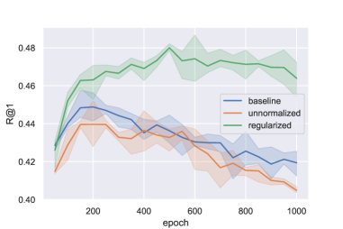
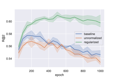
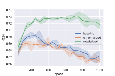
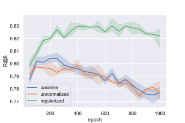
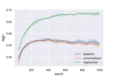
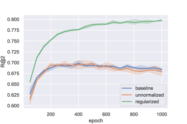
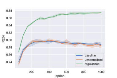
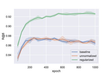
For this experiment we trained 64-dimensional encodings, again using an ImageNet pretrained GoogLeNet backbone. As in the previous section, we weigh the regularization loss by $\lambda_{1}=1$. For baselines we take the standard, normalized triplet training (denoted “baseline” in the plots) as well as the case of MTriplet with $n=1,\lambda_{1}=0$ (denoted “unnormalized” in the plots) to control that the performance improvement is due to the regularization and not that we use unnormalized embedding vectors. We train for 1,000 epochs three times in each case and report in figures 3 and 4 the evaluation metrics on the test set as a function of epochs trained. For CUB-200, our results are slightly under the state-of-the art results (using 64 dimensional embeddings with a GoogLeNet backbone) reported in Xuan et al. (2020), while for Stanford Cars we outperform the other algorithms at R@4 and R@8.

Figure 3: Test set performance vs. number of epochs trained, on the CUB-200 dataset.

Figure 4: Test set performance vs. number of epochs trained, on the Stanford Cars dataset.

4 Conclusion

We presented a method for adjusting representation learning algorithms to learn an atlas of a manifold instead of mapping into a Euclidean space. This allows, for a given encoding dimension, more interesting geometries of the embedding space. Our experiments with SimCLR and triplet-loss based metric learning training show that for low encoding dimensions our approach gives much more powerful representations over the baseline. Independent of manifold learning, we also showed that triplet loss training is significantly enhanced by adding a regularizing MMD loss function encouraging the embedding space to be uniform. We hope that this work leads to further research into atlas based manifold learning techniques.

Appendix A Appendix

A.1 Experiments setup

We ran our experiments using PyTorch Paszke et al. (2019). In all cases we use a batch size of 128 and the Adam optimizer with learning rate $10^{-4}$ and $\beta_{1}=0.9,\beta_{2}=0.999$ (the PyTorch defaults). For MNIST and FashionMNIST we use a ResNet18 He et al. (2016) backbone and train for 100 epochs while for CIFAR10 we use a ResNet50 backbone and train for 1,000 epochs. We use the same data augmentation used in the CIFAR10 experiments in the original work Chen et al. (2020a): color jitter with strength 0.5 (and a probability of 0.8 of applying), random grayscale with probability 0.2, and a random resized crop.

Each of the datasets comes with a standard train/test split. For hyperparameter selection of $\lambda_{1},\lambda_{2}$, and $\tau$ (the temperature used in the contrastive loss function) we do a grid search (with $d=2,n=16$) over $\lambda_{1}\in\{0.1,1,5,10,20\},\lambda_{2}\in\{0.05,0.1,0.2\}$, and $\tau\in\{0.1,0.5,1\}$ by training on a random selection of 80% of the training data and then computing the piece-wise linear evaluation on the remaining 20%. For MNIST and FashionMNIST we chose the hyperparameters that give the best average rank across the two datasets. This yielded $\lambda_{1}=20,\lambda_{2}=0.1$, and $\tau=1$ for MNIST and FashionMNIST and $\lambda_{1}=20,\lambda_{2}=0.1$, and $\tau=0.5$ for CIFAR10. Using these parameters we train on the entire train dataset across $d\in\{2,4,8\}$ (we noticed for higher $d$ there is not much improvement over the baseline) and $n\in\{1,4,16,32\}$. We also train baseline SimCLR for comparison (but were unable to get convergence in dimension two for CIFAR10). We repeat each training configuration three times and report the mean $\pm$ std of accuracy on the holdout test set in Table 2.

A.2 Visualizations

In this section we display visualizations for each of the datasets used in our MSimCLR experiments, using a model with $d=2,n=16$. Each image corresponds to a chart and every image in the test set gets plotted at its $(x,y)$ coordinate in the chart with highest probability. The images are best viewed by zooming in.

A.2.1 CIFAR10

A.2.2 Fashion MNIIST

We note that in this case only 15 charts are displayed since the network did not end up assigning any points to one of them.

A.2.3 MNIST

A.3 Proof of proposition 1

Proof.

We breakdown the three terms defining $\operatorname{MMD}$ (4). For the first term, we have:

$$\mathbb{E}_{(z_{1},i),(z_{2},j)\sim p\times p} k_{\mathcal{Z}}((z_{1},i),(z_{2},j))$$

$$=\mathbb{E}_{x,\tilde{x}\sim p_{\text{data}}\times p_{\text{data}}}\sum_{i,j=1}^{n}q_{i}(x)q_{j}(\tilde{x})k_{\mathcal{Z}}((\phi_{i}(x),i),(\phi_{j}(\tilde{x}),j))$$

$$=\mathbb{E}_{x,\tilde{x}\sim p_{\text{data}}\times p_{\text{data}}}\sum_{i=1}^{n}q_{i}(x)q_{i}(\tilde{x})k_{0}(\phi_{i}(x),\phi_{i}(\tilde{x}))$$

$$\approx\frac{1}{N(N-1)}\sum_{\begin{subarray}{c}j,k=1\\ j\neq k\end{subarray}}^{N}\sum_{i=1}^{n}q_{i}(x_{j})q_{i}(x_{k})k_{0}(\phi_{i}(x_{j}),\phi_{i}(x_{k})),$$

where the first equality comes from (applying twice) the fact that

$$\mathbb{E}_{z,i\sim p}f(z,i)=\mathbb{E}_{x\sim p_{\text{data}}}\mathbb{E}_{z,i\sim q(\cdot|x)}f(z,i)=\mathbb{E}_{x\sim p_{\text{data}}}\sum_{i}q_{i}(x)f(\phi_{i}(x),i),\text{for any $f:\mathcal{Z}\to\mathbb{R}$}$$ (8)

and the approximation in the last line uses the U-statistic estimate

$$\mathbb{E}_{y,\tilde{y}\sim Q\times Q}h(y,\tilde{y})\approx\frac{1}{N(N-1)}\sum_{\begin{subarray}{c}j,k=1\\ j\neq k\end{subarray}}^{N}h(y_{j},y_{k})~{}~{}\text{for any $h:\mathcal{X}\times\mathcal{X}\to\mathbb{R}$},$$ (9)

which holds for any distribution $Q$ and random sample $\{y_{1},\ldots,y_{N}\}$ drawn from $Q$.

For the second term we have, letting $\mathcal{U}_{[0,1]^{d}}$ denote the uniform distribution on $[0,1]^{d}$,

$$\mathbb{E}_{(z_{1},i),(z_{2},j)\sim p\times\mathcal{U}_{\mathcal{Z}}} k_{\mathcal{Z}}((z_{1},i),(z_{2},j))$$

$$=\mathbb{E}_{x\sim p_{\text{data}}}\sum_{i=1}^{n}q_{i}(x)\mathbb{E}_{z_{2},j\sim\mathcal{U}_{\mathcal{Z}}}k_{\mathcal{Z}}((\phi_{i}(x),i),(z_{2},j))$$

$$=\mathbb{E}_{x\sim p_{\text{data}}}\sum_{i=1}^{n}q_{i}(x)\frac{1}{n}\mathbb{E}_{w\sim\mathcal{U}_{[0,1]^{d}}}k_{0}(\phi_{i}(x),w)$$

$$\approx\frac{1}{nN^{2}}\sum_{j,k=1}^{N}\sum_{i=1}^{n}q_{i}(x)k_{0}(\phi_{i}(x_{j}),w_{k}),$$

where the first equality again follows from (8) and the approximation in the last line uses the standard expected value estimator applied to each factor. Finally for the third term we again use the estimate (9) to obtain

$$\mathbb{E}_{(z_{1},i),(z_{2},j)\sim\mathcal{U}_{\mathcal{Z}}\times\mathcal{U}_{\mathcal{Z}}} k_{\mathcal{Z}}((z_{1},i),(z_{2},j))$$

$$=\mathbb{E}_{w\sim\mathcal{U}_{[0,1]^{d}}}\mathbb{E}_{\tilde{w}\sim\mathcal{U}_{[0,1]^{d}}}\sum_{i,j=1}^{n}\frac{1}{n^{2}}k_{\mathcal{Z}}((w,i),(\tilde{w},j))$$

$$=\mathbb{E}_{w\sim\mathcal{U}_{[0,1]^{d}}}\mathbb{E}_{\tilde{w}\sim\mathcal{U}_{[0,1]^{d}}}\frac{1}{n}k_{0}(w,\tilde{w})$$

$$\approx\frac{1}{nN(N-1)}\sum_{\begin{subarray}{c}j,k=1\\ j\neq k\end{subarray}}^{N}k_{0}(w_{j},w_{k}).$$

Combining these gives the right hand side of (5). ∎

References

- Andrews et al. (2002) Ben Andrews et al. Notes on the isometric embedding problem and the Nash-Moser implicit function theorem. In Surveys in analysis and operator theory, pp. 157–208. Centre for Mathematics and its Applications, Mathematical Sciences Institute, 2002.
- Bachman et al. (2019) Philip Bachman, R Devon Hjelm, and William Buchwalter. Learning representations by maximizing mutual information across views. arXiv preprint arXiv:1906.00910, 2019.
- Chen et al. (2020a) Ting Chen, Simon Kornblith, Mohammad Norouzi, and Geoffrey Hinton. A simple framework for contrastive learning of visual representations. arXiv preprint arXiv:2002.05709, 2020a.
- Chen et al. (2020b) Xinlei Chen, Haoqi Fan, Ross Girshick, and Kaiming He. Improved baselines with momentum contrastive learning. arXiv preprint arXiv:2003.04297, 2020b.
- Do et al. (2019) Thanh-Toan Do, Toan Tran, Ian Reid, Vijay Kumar, Tuan Hoang, and Gustavo Carneiro. A theoretically sound upper bound on the triplet loss for improving the efficiency of deep distance metric learning. In Proceedings of the IEEE Conference on Computer Vision and Pattern Recognition, pp. 10404–10413, 2019.
- Grattarola et al. (2019) Daniele Grattarola, Lorenzo Livi, and Cesare Alippi. Adversarial autoencoders with constant-curvature latent manifolds. Applied Soft Computing, 81:105511, 2019.
- Gretton et al. (2012) Arthur Gretton, Karsten M Borgwardt, Malte J Rasch, Bernhard Schölkopf, and Alexander Smola. A kernel two-sample test. The Journal of Machine Learning Research, 13(1):723–773, 2012.
- Grill et al. (2020) Jean-Bastien Grill, Florian Strub, Florent Altché, Corentin Tallec, Pierre Richemond, Elena Buchatskaya, Carl Doersch, Bernardo Avila Pires, Zhaohan Guo, Mohammad Gheshlaghi Azar, et al. Bootstrap your own latent-a new approach to self-supervised learning. Advances in Neural Information Processing Systems, 33, 2020.
- Harwood et al. (2017) Ben Harwood, Vijay Kumar BG, Gustavo Carneiro, Ian Reid, and Tom Drummond. Smart mining for deep metric learning. In Proceedings of the IEEE International Conference on Computer Vision, pp. 2821–2829, 2017.
- He et al. (2016) Kaiming He, Xiangyu Zhang, Shaoqing Ren, and Jian Sun. Deep residual learning for image recognition. In Proceedings of the IEEE conference on computer vision and pattern recognition, pp. 770–778, 2016.
- He et al. (2019) Kaiming He, Haoqi Fan, Yuxin Wu, Saining Xie, and Ross Girshick. Momentum contrast for unsupervised visual representation learning. arXiv preprint arXiv:1911.05722, 2019.
- Kim et al. (2018) Wonsik Kim, Bhavya Goyal, Kunal Chawla, Jungmin Lee, and Keunjoo Kwon. Attention-based ensemble for deep metric learning. In Proceedings of the European Conference on Computer Vision (ECCV), pp. 736–751, 2018.
- Kingma & Welling (2013) Diederik P Kingma and Max Welling. Auto-encoding variational Bayes. arXiv preprint arXiv:1312.6114, 2013.
- Kohli et al. (2021) Dhruv Kohli, Alexander Cloninger, and Gal Mishne. Ldle: Low distortion local eigenmaps. arXiv preprint arXiv:2101.11055, 2021.
- Korman (2018) Eric O Korman. Autoencoding topology. arXiv preprint arXiv:1803.00156, 2018.
- Korman (2021) Eric O Korman. Self-supervised representation learning on manifolds. In ICLR 2021 Workshop on Geometrical and Topological Representation Learning, 2021. URL https://openreview.net/forum?id=EofGDIGAhvR.
- Krause et al. (2013) Jonathan Krause, Michael Stark, Jia Deng, and Li Fei-Fei. 3d object representations for fine-grained categorization. In Proceedings of the IEEE international conference on computer vision workshops, pp. 554–561, 2013.
- Krizhevsky et al. (2009) Alex Krizhevsky, Geoffrey Hinton, et al. Learning multiple layers of features from tiny images. 2009.
- LeCun et al. (2010) Yann LeCun, Corinna Cortes, and CJ Burges. MNIST handwritten digit database. ATT Labs [Online]. Available: http://yann.lecun.com/exdb/mnist, 2, 2010.
- Liu et al. (2017) Weiyang Liu, Yandong Wen, Zhiding Yu, Ming Li, Bhiksha Raj, and Le Song. Sphereface: Deep hypersphere embedding for face recognition. In Proceedings of the IEEE conference on computer vision and pattern recognition, pp. 212–220, 2017.
- Makhzani et al. (2015) Alireza Makhzani, Jonathon Shlens, Navdeep Jaitly, Ian Goodfellow, and Brendan Frey. Adversarial autoencoders. arXiv preprint arXiv:1511.05644, 2015.
- Movshovitz-Attias et al. (2017) Yair Movshovitz-Attias, Alexander Toshev, Thomas K Leung, Sergey Ioffe, and Saurabh Singh. No fuss distance metric learning using proxies. In Proceedings of the IEEE International Conference on Computer Vision, pp. 360–368, 2017.
- Musgrave et al. (2020) Kevin Musgrave, Serge Belongie, and Ser-Nam Lim. A metric learning reality check. In European Conference on Computer Vision, pp. 681–699. Springer, 2020.
- Paszke et al. (2019) Adam Paszke, Sam Gross, Francisco Massa, Adam Lerer, James Bradbury, Gregory Chanan, Trevor Killeen, Zeming Lin, Natalia Gimelshein, Luca Antiga, et al. Pytorch: An imperative style, high-performance deep learning library. arXiv preprint arXiv:1912.01703, 2019.
- Pitelis et al. (2013) Nikolaos Pitelis, Chris Russell, and Lourdes Agapito. Learning a manifold as an atlas. In Proceedings of the IEEE Conference on Computer Vision and Pattern Recognition, pp. 1642–1649, 2013.
- Schroff et al. (2015) Florian Schroff, Dmitry Kalenichenko, and James Philbin. Facenet: A unified embedding for face recognition and clustering. In Proceedings of the IEEE conference on computer vision and pattern recognition, pp. 815–823, 2015.
- Sohn (2016) Kihyuk Sohn. Improved deep metric learning with multi-class n-pair loss objective. Advances in neural information processing systems, 29:1857–1865, 2016.
- Teh et al. (2020) Eu Wern Teh, Terrance DeVries, and Graham W Taylor. ProxyNCA++: Revisiting and revitalizing proxy neighborhood component analysis. arXiv preprint arXiv:2004.01113, 2020.
- Tolstikhin et al. (2017) Ilya Tolstikhin, Olivier Bousquet, Sylvain Gelly, and Bernhard Schoelkopf. Wasserstein auto-encoders. arXiv preprint arXiv:1711.01558, 2017.
- Ustinova & Lempitsky (2016) Evgeniya Ustinova and Victor Lempitsky. Learning deep embeddings with histogram loss. Advances in Neural Information Processing Systems, 29:4170–4178, 2016.
- Welinder et al. (2010) Peter Welinder, Steve Branson, Takeshi Mita, Catherine Wah, Florian Schroff, Serge Belongie, and Pietro Perona. Caltech-UCSD birds 200. 2010.
- Xiao et al. (2017) Han Xiao, Kashif Rasul, and Roland Vollgraf. Fashion-MNIST: a novel image dataset for benchmarking machine learning algorithms, 2017.
- Xuan et al. (2018) Hong Xuan, Richard Souvenir, and Robert Pless. Deep randomized ensembles for metric learning. In Proceedings of the European Conference on Computer Vision (ECCV), pp. 723–734, 2018.
- Xuan et al. (2020) Hong Xuan, Abby Stylianou, and Robert Pless. Improved embeddings with easy positive triplet mining. In The IEEE Winter Conference on Applications of Computer Vision, pp. 2474–2482, 2020.
- Zhai & Wu (2018) Andrew Zhai and Hao-Yu Wu. Classification is a strong baseline for deep metric learning. arXiv preprint arXiv:1811.12649, 2018.