Convex Sparse Blind Deconvolution

Abstract

In the blind deconvolution problem, we observe the convolution ${\bf y}={\bf a}\star{\bf x}$ of an unknown filter ${\bf a}$ and unknown signal ${\bf x}$ and attempt to reconstruct the filter and signal. The problem seems impossible in general, since there are seemingly many more unknowns in ${\bf x}$ and ${\bf a}$ than knowns in ${\bf y}$. Nevertheless, this problem arises – in some form – in many application fields; and empirically, some of these fields have had success using heuristic methods – even economically very important ones, in wireless communications and oil exploration.

Today’s fashionable heuristic formulations pose non-convex optimization problems which are then attacked heuristically as well. The fact that blind deconvolution can be solved under some repeatable and naturally-occurring circumstances poses a theoretical puzzle.

To bridge the gulf between reported successes and theory’s limited understanding, we exhibit a convex optimization problem that - assuming the signal to be recovered is sufficiently sparse - can convert a crude approximation to the true filter into a high-accuracy recovery of the true filter.

Our proposed formulation is based on $\ell^{1}$ minimization of inverse filter outputs:

$$\begin{array}[]{ll}\underset{{\bf w}\in l_{1}^{k}}{\mbox{minimize}}&\|{\bf w}\star{\bf y}\|_{\ell_{1}^{N}}\\ \mbox{subject to}&\langle\widetilde{{\bf a}},{\bf w}^{\dagger}\rangle=1.\end{array}$$

Minimization inputs include: the observed blurry signal ${\bf y}\in{\bf R}^{N}$; and $\widetilde{{\bf a}}\in{\bf R}^{k}$, an initial approximation of the true unknown filter ${\bf a}$. Here ${\bf w}^{\dagger}$ denotes the time-reverse of ${\bf w}$. Let ${\bf w}^{*}$ denote the minimizer.

We give sharp guarantees on performance of ${\bf w}^{*}$ assuming sparsity of ${\bf x}$, showing that, under favorable conditions, our proposal precisely recovers the true inverse filter ${\bf a}^{-1}$, up to shift and rescaling.

Specifically, in a large-$N$ analysis where ${\bf x}$ is an $N$-long realization of an IID Bernoulli-Gaussian signal with expected sparsity level $p$, we measure the approximation quality of the initial approximation $\widetilde{{\bf a}}$ by considering $\widetilde{{\bf e}}=\widetilde{{\bf a}}\star{\bf a}^{-1}$, which would be a Kronecker (aka $delta$) sequence if our approximation were perfect. Under the gap condition

$$\frac{|\widetilde{{\bf e}}|_{(2)}}{|\widetilde{{\bf e}}|_{(1)}}\leq 1-p,$$

we show that, in the large-$N$ limit, the $\ell^{1}$ minimizer ${\bf w}^{*}$ perfectly recovers ${\bf a}^{-1}$ to shift and scaling.

Here the multiplicative gap $\frac{|\widetilde{{\bf e}}|_{(2)}}{\widetilde{{\bf e}}|_{(1)}}\leq 1$ denotes the ratio of the first and second largest entries of $|\widetilde{{\bf e}}|$,and is a natural measure of closeness between our approximate $\delta$ sequence $\widetilde{{\bf e}}=\widetilde{{\bf a}}*{\bf a}^{-1}$ and a true $\delta$ sequence .

In words, there is a sparsity/initial accuracy tradeoff: the less accurate the initial approximation $\widetilde{{\bf a}}\approx{\bf a}$, the greater we rely on sparsity of ${\bf x}$ to enable exact recovery. To our knowledge this is the first reported tradeoff of this kind. We consider it surprising that this tradeoff is independent of dimension $N$, i.e. that the gap condition does not demand increasingly stringent accuracy with increasing $N$.

We also develop finite-$N$ guarantees of the form $N\geq O(k\log(k))$, for highly accurate reconstruction with high probability. We further show stable approximation when the true inverse filter is infinitely long (rather than finite length $k$). And we extend our guarantees to the case where the observations are contaminated by stochastic or adversarial noise, and show that the error is linearly bounded by the noise magnitude.

1 Introduction

1.1 Blind Deconvolution

Suppose we are interested in an underlying time series ${\bf x}=(x(t))$ which we cannot observe directly. What we can observe is ${\bf y}={\bf a}*{\bf x}$ where ${\bf a}$ is an unknown ‘blurring’ filter. Blind deconvolution is the problem of recovering ${\bf x}$ merely from the observed ${\bf y}$ without knowing either ${\bf a}$ or ${\bf x}$.

This problem occurs naturally in seismology and digital communications as well as astronomy, satellite imaging, and computer vision.

In its most ambitious form, the problem is literally impossible; there are simply too few data and too many unknowns. Indeed, imagine that ${\bf x}$, ${\bf y}$ and ${\bf a}$ all have $N$ entries; we observe only $N$ pieces of information (${\bf y}$) but there are $2N$ unknowns (${\bf x}$ and ${\bf a}$). Nevertheless, in some (not all) fields, heuristic approaches have occasionally led to consistent success in isolated applications; presumably such success stories exploit specialized assumptions – although not always in an explicit or recognized way, and not with rigorous understanding.

This paper, in contrast, will exhibit a set of assumptions enabling practical algorithms for blind deconvolution, backed by rigorous theoretical analysis.

1.2 The Promise of Sparsity

Central to our approach is an assumption about the sparsity of the signal ${\bf x}$ to be recovered, in which case the problem can be called sparse blind deconvolution. Sparse signals – i.e. signals having relatively few nonzero entries, arise frequently in many fields, including seismology, microscopy, astronomy, neuroscience spike identification. Even in more abstract settings such as representation learning for computer vision, it surfaces in recently popular research trends, such as single-channel convolutional dictionary learning [Bristow et al., 2013, Heide et al., 2015, Zhang et al., 2017, Zhang et al., 2018].

The sparsity of ${\bf x}$ - if it holds - would constrain the recovery problem significantly; and so possibly, sparsity can play a role in enabling useful solutions to an otherwise hopeless problem.

An inspiring precedent can be found in modern commercial medical imaging, where sparsity of an image’s wavelet coefficients enables MRIs from fewer observations than unknowns. Taking fewer observations speeds up data collection, a principle known as compressed sensing, which already benefits tens of millions of patients yearly.

1.3 Translating Heuristics into Effective Algorithms

For sparsity to reliably enable blind deconvolution, there are two apparent hurdles. First, develop an objective function which promotes sparsity of the solution. Second, develop an algorithm which can reliably optimize the objective.

Many sparsity-promoting objectives have been proposed over the years; typically they imply non-convex optimization problems. Indeed sparsity is quantified by the $\ell_{0}$ pseudo norm $\|{\bf x}\|_{0}=\#\{t:x(t)\neq 0\}$, which is the limit of $\|{\bf x}\|_{p}^{p}$ as $p\to 0$ of concave $\ell_{p}$ pseudo-norms where $p<1$.

Traditionally, non-convex problems have been viewed by mathematical scientists with skepticism; for such problems, gradient descent and its various refinements lack any guarantee of effectiveness. Still, the lack of guarantees has not stopped engineers from trying!

A noticeable success in blind signal processing was scored in digital communications, where blind equalization today benefits billions of smartphone users. Blind equalization is a form of blind deconvolution where one exploits the known discrete-valued nature of the signal ${\bf x}$ (for example the signal entries might take only two values $\{-1,1\}$). Practitioners found that if an initial guess of the equalizer (i.e. our inverse filter ${\bf a}^{-1}$) is ‘fairly good’ (in engineer-speak ‘opening the eye’ so that a ‘hint’ of the ‘digital constellation‘ becomes ‘visible’), then certain ‘discreteness-promoting’ on-line gradient methods can reliably ‘focus’ the result better and better and allow reliable recovery.

Our work identifies an analogous phenomenon in the sparsity-promoting blind deconvolution setting, however it exposes and crystallizes the phenomenon in a rigorous and dependably exploitable form.

Namely, we show that if sparsity of ${\bf x}$ holds, and if an initial guess of the filter ${\bf a}$ is ‘fairly good’ in a precise sense, then a specific convex optimization algorithm will accurately recover both the filter and the original signal.

In retrospect, our insights on sparsity-promoting blind deconvolution can be cross-applied to explain the major successes of discreteness-promoting blind equalization in modern digital communications. Namely, a direct variation of our arguments provide a related convex optimization problem for discrete-valued signals which rigorously converts a a rough initial approximation into precise recovery.

In our view these new arguments clear away some persistent fog, mystery and misunderstandings in blind signal processing; and pave the way for future success stories.

1.4 Prior Work

Searching for an inverse filter that promotes desired output properties

Instead of trying to recover ${\bf a}$ and ${\bf x}$ together from ${\bf a}*{\bf x}$, we could formulate this problem as looking for an approximate inverse filter ${\bf w}$ so that the output ${\bf w}*{\bf y}$ exhibits extremal properties. Under this formulation, our goal is to find ${\bf w}\neq 0$, so that

$$\begin{array}[]{ll}\underset{{\bf w}\neq 0}{\mbox{optimize}}&J({\bf w}\star{\bf y})\end{array}$$ (1)

where the functional $J$ quantifies the properties we seek to promote. (Depending on $J$, we might either prefer its maximum or minimum ).

Working in exploration seismology, Wiggins [Wiggins, 1978] adopted this approach with the normalized $4$-norm, $J({\bf z})=J_{4,2}={\|{\bf z}\|_{4}}/{\|{\bf z}\|_{2}}$ and gave a few successful data-processing case studies. His successful examples all clearly exhibit sparsity, although this was not discussed at the time. Other objectives considered at that time included $J_{2,1}({\bf z})=\|{\bf z}\|_{2}/\|{\bf z}\|_{1}$ and $J_{\infty,2}({\bf z})=\|{\bf z}\|_{\infty}/\|{\bf z}\|_{2}$ [Cabrelli, 1985].

It was fully understood at that time that output property optimization could succeed in principle, if one did not have to worry about an effective algorithm. [Donoho, 1981] showed that if the signal ${\bf x}$ is a realization of independent and identically distributed entries from any nonGaussian distribution, optimizing $J$ of the output ${\bf w}\star{\bf y}$ is successful in the large-$N$ setting - as long as the functional $J$ belongs to a certain large family of non-Gaussianity measures, for example including $J_{4,2}$ and $J_{2,1}$ as well as many others.

The issue left unresolved in those days was how to solve such optimization problems. Indeed optimizations like $J_{4,2}$ are badly nonconvex, as we see clearly by rewriting the $J_{4,2}$ problem as

$$\begin{array}[]{ll}\underset{{\bf w}}{\mbox{maximize}}&\|{\bf w}*{\bf y}\|_{4}\\ \mbox{subject to}&\|{\bf w}*{\bf y}\|_{2}=1.\end{array}$$

The theory cited above derived favorable properties of a would-be procedure which truly finds the optimum of a badly nonconvex objective. It clarifies that blind deconvolution is possible in principle but does not by itself help us algorithmically, i.e. in practice. In the intellectual climate of the time, solving badly nonconvex optimization problems was considered a pipe dream, a time-wasting charade for non-serious people.

Even today, blind deconvolution continues to be studied as an non-convex optimization problem; see recent work [Kuo et al., 2019, Kuo et al., 2020, Lau et al., 2019], who study the problem of recovering short $a$ and sparse $x$

Blind equalization

In digital communications, the transmitted signal ${\bf x}$ can be viewed as discrete-alphabet valued; for example, in PAM signaling, where $x(t)\in\{\pm 1\}$, and QAM signaling, where the signal alphabet has equally spaced points on unit sphere in complex space [Kennedy and Ding, 1992, Ding and Luo, 2000].

[Vembu et al., 1994] considered the non-convex problem

$$\begin{array}[]{ll}\underset{{\bf w}}{\mbox{maximize}}&\|{\bf w}*{\bf y}\|_{8}\\ \mbox{subject to}&\|{\bf w}*{\bf y}\|_{2}=1\end{array}$$

If the data ${\bf y}$ were preprocessed to be serially uncorrelated, this optimization is effectively of the earlier form $J_{8,2}$.

The authors attack this nonconvex problem using projected gradient descent and give suggestive experimental results. They apparently view the $\ell_{8}$ norm objective as an approximation of the $\ell_{\infty}$ norm objective $\|{\bf w}*{\bf y}\|_{\infty}$. Later, [Ding and Luo, 2000] used linear programming to solve the $\infty$ norm problem directly.

Searching for a projection with desired output properties

Here is another setting for property-promoting output optimization. We have a data matrix $Y\in{\bf R}^{n,p}$ - which we think of as $n$ points in ${\bf R}^{p}$, and we have a unit vector $w\in{\bf R}^{p}$ called the projection direction. Our output vector $Y\cdot w$ contains the projection of the $n$-points on the projection direction q; it has $n$ entries. We seek ‘interesting’ projections; i.e. directions where the projection displays some structure. We adopt a functional $J$ which measures properties we seek to promote in the output, and we seek to solve:

$$\begin{array}[]{ll}\underset{\|w\|=1}{\mbox{optimize}}&J(Y\cdot w).\end{array}$$ (2)

This was implemented by [Friedman and Tukey, 1974], who proposed a functional that promotes ‘clumping’ or ’clustering’ of the output. They called it projection pursuit and were motivated by exploratory high dimensional data analysis; for $p$-dimensional data involve $p>2$ and we can’t easily get a visual sense of what’s in the data. It was hoped at the time that looking at selected low-dimensional projections might lead to better insights. For the most part, such hopes for exploration of high-dimensional data never materialized.

However, output optimization of this type has proven to be useful in important problems in blind signal processing, where $Y$ has known structure that can be exploited systematically.

In blind source separation we observe $Y=XA$, $Y\in{\bf R}^{n,p}$, $X\in{\bf R}^{n,p}$ and $A\in{\bf R}^{p,p}$ is an invertible matrix. (We don’t observe $X$ or $A$ separately).

Think of the $X$ matrix as containing columns giving successive time samples of $p$ clean source signals, for example $p$ individual acoustic signals. These signals arrive at array of $p$ spatially distributed acoustic sensors, each of which records the acoustic information it receives. The matrix $Y$ contains in its columns what was obtained by each of the $p$ different sensors. In general, each sensor receives information from each of the sources. This is colorfully called the cocktail party problem, referring to the setting where $X$ records the sources are human speakers at a cocktail party, and $Y$ records what is heard at various locations in a room. Each column of $Y$ then contains a superposition of different speakers; while we would prefer to separate these and pay attention to just the ones of most immediate interest to us.

In this separation problem, sparsity of the signal might be valuable. Suppose that each individual speaker is listening quite a bit and so not speaking much of the time. Then the columns of $X$ are each sparse. On the other hand, if there are many people in the room, the room as a whole may still always be noisy, and so each column of $Y$ may be fully dense. Assuming $A$ is invertible, and the vector $w$ obeys $Aw=e_{j}$, then $Y\cdot w$ extracts column $j$ of $X$, which will be sparse. Hence, we may hope that the projection pursuit principle, with an appropriate measure $J$, might identify the ‘sparse’ projections we seek.

Ju Sun, Qu Qing, Yu Bai, John Wright, Zibulevsky and Pearlmutter [Sun et al., 2015, Sun et al., 2016, Bai et al., 2018, Zibulevsky and Pearlmutter, 2000] proposed the optimization problem

$$\begin{array}[]{ll}\underset{w}{\mbox{minimize}}&\|Yw\|_{1}\\ \mbox{subject to}&\|w\|_{2}=1.\end{array}$$

Assuming the $Y$ data pre-processed so that $\frac{1}{n}Y^{\prime}Y=I_{p}$ this is equivalent to projection pursuit (2) applied to the objective $J_{2,1}$. Notably, this is again a highly non-convex optimization problem.. The authors proposed projected gradient descent and recited some favorable empirical results.

There is a close relation between the blind deconvolution optimization (1) and the projection pursuit optimization (2). Indeed, if the $Y$ matrix is filled in from an observed time series appropriately, then output optimization in blind deconvolution and in projection pursuit are essentially identical. Namely, let ${\bf y}^{ser}=(y^{ser}(t))_{t=1}^{N}$ denote a time series of interest to us, and $Y^{mat}=(Y^{mat}_{i,j})$ denote an $n\times p$ matrix where $n=N-p$ constructed using ${\bf y}^{ser}$ like so:

$$Y^{mat}_{i,j}=y^{ser}(p+i-(j-1)),\qquad 1\leq i\leq n=N-p;\;1\leq j\leq p.$$

Now suppose the filter vector ${\bf w}$ in the blind deconvolution optimization and the projection direction $w$ in the projection pursuit optimization are chosen identically. Then the blind deconvolution output objective $J({\bf w}\star{\bf y}^{ser})$ is identical to the projection pursuit objective $J(Y^{mat}w)$, except for possibly different treatment of the first $p$ entries of ${\bf y}^{ser}$.

Convex Projection Pursuit

In view of the connection between blind deconvolution and projection pursuit, and in view of our results in this paper, it is quite interesting to consider the work of [Spielman et al., 2012] and [Gottlieb and Neylon, 2010]. They propose to solve the following linear-constrained convex optimization problem. Given an $n\times p$ data matrix $Y$ and a constraint vector $u$, they propose to solve:

$$\begin{array}[]{ll}\underset{w}{\mbox{minimize}}&\|Yw\|_{1}\\ \mbox{subject to}&u^{T}w=1.\end{array}$$

As it turns out, when the matrix $Y$ in this problem and ${\bf y}$ in the time series deconvolution problem are related by the $Y^{mat}$-${\bf y}^{ser}$ construction just mentioned, the objective we propose in this paper is essentially identical, when $\tilde{{\bf a}}=u$. As we will show, our setting permits much more thorough studies and more penetrating analyses, and we find that success in sparse blind deconvolution is more broadly prevalent than one might have expected, based on earlier analyses such as [Spielman et al., 2012] or [Sun et al., 2015, Sun et al., 2016, Bai et al., 2018, Zibulevsky and Pearlmutter, 2000] .

1.5 Mathematical setup

Sequence Space, and Filtering

To make our results concrete, let’s discuss things formally. Let ${\mathbf{X}}$ denote the collection of bilaterally infinite sequences ${\bf x}=(x(t):t=0,\pm 1,\pm 2,\dots)$; for short we call such objects bisequences. Then $\ell_{1}({\mathbb{Z}})\subset{\mathbf{X}}$ denotes the collection of bisequences obeying $\|{\bf x}\|_{1}=\sum_{t}|x(t)|<\infty.$ For a bisequence ${\bf x}$ we denote time reversal operator $t\leftrightarrow-t$ by ${\bf x}^{\dagger}$. For whole number $k>0$ let ${\mathbf{X}}_{k}$ denote the subspace of bisequences supported in $-k\leq t\leq k$. We sometimes abuse notation: for a bisequence ${\bf x}$ we might write ${\bf x}=(1,.3)$ when we really mean ${\bf x}=(\ldots,0,0,1,.3,0,0,\ldots)$.

Let $\star$ denote the convolution product on pairs of bisequences in $\ell_{1}({\mathbb{Z}})$ - $({\bf x}\star{\bf y})=\sum_{u}x(t-u)y(u)$. Let ${\bf e}_{0}$ denote the ‘delta’ or ‘Kronecker’ bisequence: ${\bf e}_{0}(t)=1_{\{t=0\}}$; ${\bf e}_{0}$ is the unit of convolution. The convolution inverse of ${\bf x}$ $\--$ ${\bf x}^{-1}$ $\--$ is a bisequence obeying ${\bf x}\star{\bf x}^{-1}={\bf e}_{0}$. For example, the filter ${\bf x}=(\dots,0,1,1/2,1/4,1/8,\ldots)$ anchored at the time origin so ${\bf x}(0)=1$, has inverse ${\bf x}^{-1}=(\dots,0,1,-1/2,0,\dots)$, again anchored at the time origin. Abusing notation we may simply write ${\bf x}^{-1}=(1,-1/2)$.

Our approach to blind deconvolution searches among candidates for a filter ($\equiv$ bisequence) that extremizes a certain objective function. We then show that the extremal is in fact the desired inverse filter to our (unknown) true underlying filter. Hence, it helps know conditions under which an inverse filter actually exists!

For a bisequence ${\bf x}\in\ell_{1}({\mathbb{Z}})$, we define the Fourier transform $\hat{{\bf x}}(w)=\mathcal{F}{\bf x}(w)\equiv\sum_{t}x(t)\exp\{i2\pi wt\}$. For the inverse transform, we use $x(t)=(\mathcal{F}^{-1}\hat{{\bf x}})(t)=\frac{1}{2\pi}\int_{0}^{2\pi}\hat{{\bf x}}(w)\exp\{-i2\pi wt\}dw$.

Lemma 1.1 (Wiener’s lemma).

If ${\bf a}\in\ell_{1}({\mathbb{Z}})$, and also $(\mathcal{F}{\bf a})(\widetilde{w})\neq 0$, $\forall\widetilde{w}\in T$, then an inverse filter exists in $\ell_{1}({\mathbb{Z}})$. The bilaterally infinite sequence defined formally by

$${\bf a}^{-1}:=\mathcal{F}^{-1}(\frac{1}{\mathcal{F}{\bf a}})$$

exists as an element of $\ell_{1}({\mathbb{Z}})$ and obeys ${\bf a}^{-1}*{\bf a}={\bf e}_{0}.$

In the engineering literature, we say that the bisequence ${\bf a}$ has so-called $Z$-transform $A(z)$, defined by:

$$\begin{array}[]{ll}A(z)=\sum_{t=-\infty}^{\infty}a_{t}z^{-t}.\end{array}$$

Evaluating $A$ on the unit circle in the complex plane, at $z$ of the form $z=\exp\{-i2\pi w\}$, we see that the $Z$-transform is effectively the Fourier transform $A={\cal F}{\bf a}$. Applying Wiener’s lemma, we see that, if ${\bf a}\in\ell_{1}$ and $\min_{w}|A(\exp\{-2\pi iw\})|>0$, i.e. $A$ is never zero on the unit circle, then ${\bf a}^{-1}\in\ell_{1}$ and $1/A$ is the $Z$-transform of ${\bf a}^{-1}$.

Finite-sample observation model and finite-length inverse filter

In searching for an inverse filter, our initial results assume existence of a finite-length inverse. Namely, we assume that ${\bf a}\in\ell_{1}({\mathbb{Z}})$ is a forward filter with an inverse filter ${\bf a}^{-1}\in\ell_{1}({\mathbb{Z}})$ supported in a centered window of radius $k$.

In practice we only have a finite dataset! Suppose that there is an underlying bisequence ${\bf y}\in{\mathbf{X}}$ of the form ${\bf y}={\bf a}*{\bf x}$, and let ${\bf y}^{[N]}$ denote the restriction to an $N$-long centered window ${\cal T}=\{-T,\dots,T\}$ of radius $T$ and size $N=2T+1$.

Our goal is seemingly to recover ${\bf x}$ or ${\bf a}$ from the observed data ${\bf y}^{[N]}$. However, in statistical theory we generally don’t expect to exactly recover the true underlying representation (i.e. the generating ${\bf a}$ and ${\bf x}$) exactly. Our goal is instead to find an inverse filter ${\bf w}\in\ell_{1}^{k}$ such that the convolution ${\bf w}*{\bf y}$ would be close to ${\bf x}$, and where the closeness improves with increasing data size $N\to\infty$.

Finite-length filtering and practical algorithms

While our analysis framework concerns bisequences (bilaterally infinite sequences), our data have finite length (as just mentioned). The algorithms we discuss are often motivated by convolutions on bisequences; however, they reduce in practice to truncated convolutions involving finite data windows. A certain ambiguity is helpful for efficient communication. Suppose we have ${\bf y}^{[N]}$, an N-long observed window of ${\bf y}$, and we also have ${\bf w}$, a k-long filter, by which we mean a bisequence nonzero only within a fixed $k$-long window. We might encounter discussion both of ${\bf w}\star{\bf y}^{[N]}$ as well as ${\bf w}\star{\bf y}$, both using the same filter ${\bf w}$. In the first case, we would actually be thinking of ${\bf y}^{[N]}$ as zero-padded out to a bisequence, so that both situations involve bisequence convolutions.

Finite $N$ effects are important in practice but tedious to discuss. It can be important to account for end effects in truncated convolution. In a setting where we initially think to consider a norm $\|{\bf w}\star{\bf y}^{[N]}\|_{\ell_{p}({\mathbb{Z}})}$, we might instead next think to rather consider the windowed norm $\|{\bf w}\star{\bf y}^{[N]}\|_{\ell_{p}(\{-T,\dots,T\})}$, while finally we realize $\|{\bf w}\star{\bf y}^{[N]}\|_{\ell_{p}(\{-T+k,\dots,T-k\})}$ is more correct for our purposes, as it includes only the terms which do not suffer from truncation of the convolution.

Algorithmic formulation

Under assumptions we will be making, the sequence ${\bf x}$ underlying our observed data will be either exactly sparse – having few nonzeros – or approximately so. Moreover, there will be either an exact length $k$ inverse filter ${\bf w}$, or approximately such. It follows that the filter output ${\bf w}\star{\bf y}$ is sparse. This suggests the would-be optimization principle

$$\begin{array}[]{ll}\underset{{\bf w}\neq 0}{\mbox{minimize}}&\|{\bf w}\star{\bf y}^{[N]}\|_{\ell_{0}(\{-T+k,\dots,T-k\}})\end{array}$$

where the $\ell_{0}$ quasi-norm simply counts the number of nonzero entries. Unfortunately, this objective, though well-motivated, is not suitable for numerical optimization.

Inspired by this, we perform convex relaxation of the $\ell_{0}$ norm, replacing it with the $\ell_{1}$ norm, which is convex.

We also need to fix the scale to get a unique output. One might think to constrain $\|{\bf w}\|_{2}=1$, however, this would give a non-convex constraint and again is not suitable for effective algorithms.

We instead suppose given a rough initial approximation $\widetilde{{\bf a}}$ of the forward filter ${\bf a}$, and impose an $\ell_{\infty}$ constraint on the ‘pseudo-delta’ ${\bf w}\star\widetilde{{\bf a}}$, forcing it to ‘peak’ at target entry $t$.

$$\begin{array}[]{ll}&(\widetilde{{\bf a}}*{\bf w})_{t}=1,\quad\|\widetilde{{\bf a}}*{\bf w}\|_{\infty}\leq 1.\end{array}$$ (3)

Combining these steps, we obtain a convex optimization problem associated to each possible target coordinate $t$:

$$\begin{array}[]{ll}\underset{{\bf w}\in\ell_{1}^{k}}{\mbox{minimize}}&\frac{1}{N-2k}\|{\bf w}\star{\bf y}^{[N]}\|_{\ell_{1}(\{-T+k,T-k\})}\\ \mbox{subject to}&(\widetilde{{\bf a}}*{\bf w})_{t}=1,\quad\|\widetilde{{\bf a}}*{\bf w}\|_{\infty}\leq 1.\end{array}$$ (4)

It will be convenient to reformulate slightly, hide consideration of end effects, and force the peak to occur at target coordinate $t=0$. Abusing notation somewhat, we then write:

$$\begin{array}[]{ll}\underset{{\bf w}\in\ell_{1}^{k}}{\mbox{minimize}}&\frac{1}{N}\|{\bf w}*{\bf y}\|_{\ell_{1}^{N}}\\ \mbox{subject to}&\langle\widetilde{{\bf a}},{\bf w}^{\dagger}\rangle=1,\end{array} {C}_{\widetilde{{\bf a}}}$$ ( )

(Again ${\bf w}^{\dagger}$ denotes time-reversal of ${\bf w}$). In practice we might truncate the convolution due to end effects, or truncate the window over which we take the norm, but we will hide such practical details in the coming material, for ease of exposition; they would not change our results.

Stochastic models for sparse signals

Although our algorithms make sense in the absence of any theory, our theoretical results concern properties of our algorithm for data generated under a probabilistic generative model i.e. a stochastic signal model.

Let $X=(X_{t})$ be a bisequence of independent identically distributed random variables indexed by $t\in{\mathbb{Z}}$, having a common marginal CDF $F=F_{X}$, such that $F(x)=1-F(-x)$. One realization is then a sequence ${\bf x}$ of the type discussed in earlier paragraphs.

We assume that $F$ has an atom at $0$ - $F=(1-p)H+pG$, where $H$ is the standard Heaviside distribution and $G$ is the standard Gaussian distribution. We say that $F$ follows the Bernoulli$(p)$-Gaussian model. Equivalently, $X_{t}$ is sampled IID from the Bernoulli$(p)$-Gaussian distribution $pN(0,1)+(1-p)\delta_{0}$.

The iid process $X$ is of course ergodic. If ${\bf x}$ denotes one realization of $X$, then in a window $(x_{t})_{-T}^{T}$ of length $N$, $\approx pN$ nonzero values will occur, for large $N$. Consequently, if $p\ll 1$, realizations from $X$ will empirically be sparse.

Let $Y={\bf a}\star X$ denote the random bisequence produced as the output of convolution of the random signal $X$ with deterministic filter ${\bf a}\in\ell_{1}({\mathbb{Z}})$. More explicitly,

$$Y_{t}=\sum_{u}a(u)X_{t-u}.$$

This defines formally a so-called stationary linear process, a classical object for which careful foundational results are well established. Consider now filtering $Y$, by a length-$k$ filter ${\bf w}$, producing the random bisequence $V={\bf w}\star Y$. The end-to-end filter ${\bf b}={\bf w}\star{\bf a}$ is a well-defined element of $\ell_{1}({\mathbb{Z}})$; using it, we can represent the filtered output in terms of the underlying iid process $X$: $V={\bf b}\star X$. This representation shows that the filtered output series $V$ is itself a well-defined stationary linear process, and moreover, since $E|X_{0}|<1$ and $\|{\bf b}\|_{\ell_{1}}\leq\|{\bf w}\|_{\ell_{1}}\cdot\|{\bf a}\|_{\ell_{1}}<\infty$, we have $E|V_{0}|<\|{\bf b}\|_{\ell_{1}}<\infty$.

Any such stationary linear process is ergodic. By the ergodic theorem, the large-$N$ limit of the objective will almost surely be an expectation over $X$:

$$\begin{array}[]{ll}\lim_{N\rightarrow\infty}\frac{1}{N}\|{\bf w}*Y\|_{\ell_{1}^{N}}=\lim_{N\rightarrow\infty}\frac{1}{N}\sum_{t\in{\cal T}^{N}}|({\bf b}\star X)_{t}|={\mathbb{E}}_{X}|({\bf b}\star X)_{0}|={\mathbb{E}}|({\bf w}*Y)_{0}|.\end{array}$$ (5)

Consequently, the large-$N$ properties of our proposed algorithm are driven by properties of the following optimization problem in the population:

$$\begin{array}[]{ll}\underset{{\bf w}}{\mbox{minimize}}&{\mathbb{E}}|({\bf w}*Y)_{0}|\\ \mbox{subject to}&\langle\widetilde{{\bf a}},{\bf w}^{\dagger}\rangle=1.\end{array}$$

2 Main Results Overview

2.1 Main Result $1$: Phase Transition Phenomenon for Sparse Blind Deconvolution

We have at last defined a convex optimization problem at the population level, which we will now want to study in detail. In our studies, we can make various choices of the sparsity parameter $p$, of the underlying forward filter ${\bf a}$, and of the guess $\tilde{{\bf a}}$. The tuple $(p,{\bf a},\tilde{{\bf a}})$ defines in this way a kind of phase space. We can then study performance of the algorithm at different points in phase space.

Consider this performance property:

ExactRecovery  $\equiv$   “There is an unique solution of the population-based optimization problem — modulo time shift and output rescaling — and this solution exactly solves the blind deconvolution problem correctly. ”

It probably seems too much to ask that such a property could ever be true, i.e. could ever be true for even one choice of phase space tuple. After all the optimization problem doesn’t have any apparent connection to blind deconvolution – instead only to some sort of relaxation of the search for sparse output filters.

We will see that this phase space can be partitioned into two regions: one where the exact recovery property holds and its complement where the exact recovery property fails. Surprisingly the region where ExactRecovery  holds is nonempty and can be appreciable. And it can be described in a clear and insightful way.

Surprising phase transition for a special case of sparse blind deconvolution

We first illustrate the phase transition phenomenon in possibly the most elementary situation. Consider the special case when the forward filter ${\bf a}$ is the exponential decay filter: ${\bf a}=(1,s,s^{2},s^{3},\ldots)$ with $|s|\leq 1$; then the inverse filter is a basic short filter ${\bf a}^{-1}=(1,-s)$.

Theorem 1 (Population phase transition for exponential decay filter).

Consider a linear process $Y={\bf a}*X$ with

• ${\bf a}=(1,s,s^{2},s^{3},\ldots)$ where $|s|\leq 1$, so ${\bf a}^{-1}=(1,-s)$;

• $X_{t}$ is IID Bernoulli$(p)$-Gaussian $pN(0,1)+(1-p)\delta_{0}$.

Consider as initial approximation $\widetilde{{\bf a}}={\bf e}_{0}=(1,0,0,0,\ldots)$, and the resulting fully specified population optimization problem, with parameter tuple $(p,{\bf a},\tilde{{\bf a}})$:

$$\begin{array}[]{ll}\underset{{\bf w}}{\mbox{minimize}}&{\mathbb{E}}|({\bf w}*Y)_{0}|\\ \mbox{subject to}&{\bf w}_{0}=1.\end{array}$$

Let ${\bf w}^{\star}$ denote the (or simply some) solution. Define the threshold

$$p^{\star}=1-|s|.$$

The property ExactRecoveryexperiences a phase transition at $p=p^{\star}$:

• provided $p<p^{\star}$, then ${\bf w}^{\star}$ is uniquely defined and equal to ${\bf a}^{-1}$ up to shift and scaling ; and

• provided $p>p^{\star}$, then ${\bf w}^{\star}$ is not ${\bf a}^{-1}$ up to shift and scaling .

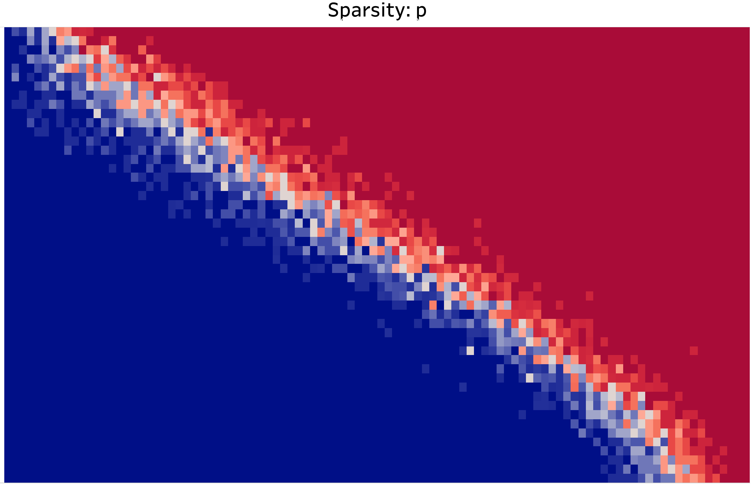
Figure 1: Finite-sample phase transition diagram; ground truth filter is ${\bf w}^{\star}=(0,1,-s)$ with $T=200$. Horizontal axis: sparsity level $p$, ranging from $0.01$ to $0.99$; Vertical axis: filter parameter $|s|$, ranging from $0$ to $0.99$. The shaded attribute indicates the observed fraction of successful experiments at the given parameter combination from deep blue for 1.0 down to deep red for 0.0. Thus, the red region indicates failure of recovery and the blue region indicates success. The transition from success to failure is quite abrupt.

We can empirically observe that the population phase transition described in Theorem 1 describes accurately the situation with finite-length signals. The setting of Theorem 1, defines a phase space by the numbers $(p,s)$. We can sample the phase space according to a grid and then at each grid point, conducting a sequence of experiments like so:

• sample a realization of synthetic data $Y={\bf a}\star X$ according to the stochastic signal;

• extract a window ${\bf y}^{[N]}$ of size $N$ from within each generated $Y$; and

• solve the resulting finite-$N$ optimization problem:

  $$\begin{array}[]{ll}\underset{{\bf w}}{\mbox{minimize}}&\frac{1}{N}\|{\bf w}*Y\|_{1}\\ \mbox{subject to}&{\bf w}_{0}=1.\end{array}$$

Tabulating the fraction of instances with numerically precise recovery of the correct underlying inverse filter ${\bf a}^{-1}$ and sparse signal $X$ across grid points, we can make a heatmap of empirical success probability.

Specifically, we numerically run $20$ independent experiments, and choose an accuracy $\epsilon=10^{-3}$ and count the number of successfully accurate recovery where the convex optimization solution $w$ satisfy $\|w^{\star}-w\|_{1}/\|w^{\star}\|_{\infty}<\epsilon$.

We do this in Figure 1; the reader will see there an empirical phase transition curve, produced by a logistic-regression calculation of the location in $p$ where $50\%$ success probability is achieved. We observe empirical behavior entirely consistent with $p^{\star}=1-|s|$.

Phase transition for sparse blind deconvolution with general filter: upper bound from deltaness discrepancy

Consider now a more general situation where ${\bf a}$ is a quite general filter, and $X$ is Bernoulli Gaussian. Our formal assumptions are:

1. ${\bf a}\in l_{1}({\mathbb{Z}})$ is invertible: $(\mathcal{F}{\bf a})(\widetilde{w})\neq 0$, $\forall\widetilde{w}\in T$; thus ${\bf a}^{-1}$ exists in $\ell_{1}({\mathbb{Z}})$.

2. $X=(X_{t})_{t\in{\mathbb{Z}}}$ is IID with marginal distribution $pN(0,1)+(1-p)\delta_{0}$; and

3. $Y=(Y_{t})_{t\in{\mathbb{Z}}}$ is a linear process obeying $Y={\bf a}\star X$.

Consider the convex optimization problem

$$\begin{array}[]{ll}\underset{{\bf w}\in l_{1}({\mathbb{Z}})}{\mbox{minimize}}&{\mathbb{E}}|({\bf w}*Y)_{0}|\\ \mbox{subject to}&\langle\widetilde{{\bf a}},{\bf w}^{\dagger}\rangle=1,\end{array}$$

and let ${\bf w}^{\star}$ denote any solution of the optimization problem.

Our results establish the existence of a general phase transition phenomenon and a precise quantification of it, in terms of a phase transition functional .

Define the following deltaness discrepancy $\Delta({\bf v})$:

$$\Delta({\bf v})=\inf_{\alpha,k}\frac{\|{\bf v}-\alpha\delta_{k}\|_{\infty}}{\|{\bf v}\|_{\infty}}.$$

This discrepancy indeed obeys $\Delta({\bf e}_{0})=0$. However, it is not restricted only to deltaness concentrating at the origin; in fact, $\Delta(\alpha\cdot{\bf e}_{k})=0$ for each $\alpha>0$, $k\in{\mathbb{Z}}$. Also, $0\leq\Delta({\bf v})\leq 1$. At the other extreme, $\Delta([...,0,0,1/2,1/2,0,0,...])=1$. Finally, $\Delta$ is a continuous function on $l_{1}({\mathbb{Z}})$: so that, setting ${\varepsilon}({\bf v},{\bf w})\equiv\frac{\|v-w\|_{\infty}}{\|w\|_{\infty}}$,

$$|\Delta({\bf v})-\Delta({\bf w})|\leq\frac{2\cdot{\varepsilon}}{1-{\varepsilon}}.$$

Indeed, we can give a more explicit form for $\Delta$; let $\widetilde{{\bf e}}:=\widetilde{{\bf a}}*{\bf a}^{-1}$,

$$\Delta(\widetilde{{\bf e}})=\frac{|\widetilde{{\bf e}}|_{(2)}}{|\widetilde{{\bf e}}|_{(1)}},$$

where $|\widetilde{{\bf e}}|_{(1)}$ denotes the largest entry in $\widetilde{{\bf e}}$ and $|\widetilde{{\bf e}}|_{(2)}$ the second largest. $\frac{|\widetilde{{\bf e}}|_{(2)}}{|\widetilde{{\bf e}}|_{(1)}}$ is a kind of multiplicative gap functional, measuring the extent to which the second-largest entry in $\widetilde{{\bf e}}$ is small compared to the largest entry. It is a natural measure of closeness between our approximate Kronecker delta $\widetilde{{\bf e}}=\widetilde{{\bf a}}*{\bf a}^{-1}$ and true Kronecker delta ${\bf e}_{0}$.

Theorem 2 ( Population (large-$N$) phase transition: upper bound from deltaness discrepancy).

Under assumptions (A1)-(A3),

• There is a functional $\Pi^{*}$ defined on tuples $({\bf a},\widetilde{{\bf a}})$ in $\ell_{1}({\mathbb{Z}})\times\ell_{1}({\mathbb{Z}})$ with the property that, for $p>\Pi^{*}({\bf a},\widetilde{{\bf a}})$, every solution of the optimization problem ${P}_{1}(\widetilde{{\bf a}})$ is exactly the correct answer ${\bf a}$, up to lateral shift and scaling.

• We have the upper bound:

  $$\Pi^{*}({\bf a},\widetilde{{\bf a}})\leq 1-\Delta(\widetilde{{\bf a}}*{\bf a}^{-1}),\qquad({\bf a},\widetilde{{\bf a}})\in\ell_{1}({\mathbb{Z}})\times\ell_{1}({\mathbb{Z}}).$$ (5)

  In words, the theorem is stating that the less accurate the initial approximation $\widetilde{{\bf a}}\approx{\bf a}$, the greater we rely on sparsity of $X$ to allow exact recovery.

The reader might compare this with our earlier example in Theorem 1, the special case of geometrically decaying filters. In that example ${\bf a}=(\dots,0,0,1,s,s^{2},\dots)$ while $\widetilde{{\bf a}}=(\dots,0,0,1,0,0,\dots)$. $\Delta(\widetilde{{\bf a}}*{\bf a}^{-1})=\Delta((\dots,0,0,1,s,s^{2},\dots))=|s|$. In short, the upper bound $\Pi^{*}=1-|s|$ deriving from this general viewpoint agrees precisely with the the exact answer $p^{*}=1-|s|$ given in that earlier Theorem.

When does equality hold in (5)? For a vector ${\bf v}$, let ${\bf v}^{\prime}$ denote the same vector, except the largest-amplitude entry is replaced by $0$. We will see that a sufficient condition for equality is:

$$\Delta(\widetilde{{\bf e}}^{\prime})\leq\Delta(\widetilde{{\bf e}}).$$

Put another way, equality holds if

$$|\widetilde{{\bf e}}|_{(3)}\leq\Delta(\widetilde{{\bf e}})\cdot|\widetilde{{\bf e}}|_{(2)}.$$ (6)

The set of situations where this occurs is ample but not overwhelming. It has relative Lebesgue measure at least $\Delta$. In the situation covered by Theorem 1, $|\widetilde{{\bf e}}|_{(3)}=s^{2}$, $|\widetilde{{\bf e}}|_{(2)}=s$, $\Delta=s$, and so equality holds in (6). Hence, the general-filter result of Theorem 2 along with the sufficient condition (6) imply as a special case Theorem 1.

Now we state the following corollary to show that there is a substantial region in the space of $({\bf a},\widetilde{{\bf a}})$ pairs where a meaningful sparsity-accuracy of initialization tradeoff exists, such that any sufficiently accurate initial guess results in exact recovery - provided that the sparsity of the underlying object $X$ exceeds a threshold.

Corollary 2.1.

Let $r\in(0,1/2)$ and suppose that assumptions (A1)-(A3) hold with $p>\frac{r}{1-r}$. Normalize the problem so that $\|{\bf a}^{-1}\|_{\infty}=1$.

Consider $\widetilde{{\bf a}}$ in the $\ell_{1}$ metric ball (7) of radius $r$ about ${\bf a}$:

$$\|\widetilde{{\bf a}}-{\bf a}\|_{1}\leq r.$$ (7)

Every solution of the optimization problem $P_{1}(\widetilde{{\bf a}})$ achieves exact recovery of ${\bf a}$ up to shift and rescaling.

Proof: Since

$$\|\widetilde{{\bf e}}-{\bf e}_{0}\|_{\infty}\leq\|{\bf a}^{-1}\|_{\infty}\cdot\|\widetilde{{\bf a}}-{\bf a}\|_{1}=r,$$

we have $|\widetilde{{\bf e}}|_{(1)}\geq 1-r$ and $|\widetilde{{\bf e}}|_{(2)}\leq r.$ This implies that $\Pi^{*}\leq\frac{r}{1-r}$. Now apply theorem 2. ∎

Phase transition for sparse blind deconvolution with general filter from optimization point of view

Theorem 2 has provided a upper bound of the threshold $p^{\star}$ for phase transition with clear mathematical meaning. Now we present the main phase transition theorem with the exact $p^{\star}$ for blind deconvolution of general inverse filter. This statement is from optimization point of view that connects blind deconvolution problem to a classical projection pursuit problem.

Let $I$ denote an iid Bernoulli(p) bisequence. For a bisequence ${\bf w}$ let ${\bf w}\cdot I$ denote the elementwise multiplication of ${\bf w}$ by $I$. Define the optimization problem

$$\begin{array}[]{ll}\underset{{\bf w}}{\mbox{minimize}}&{\mathbb{E}}_{I}\|{\bf w}\cdot I\|_{2}\\ \mbox{subject to}&\langle{\bf v},{\bf w}\rangle=1\end{array}$$

Theorem 3 (Population (large-$N$) phase transition: upper and lower bound).

Under assumptions (A1)-(A3),consider the solution ${\bf w}^{\star}$ of the convex optimization problem ${P}_{1}(\widetilde{{\bf a}})$. There is a threshold $p^{\star}>0$,

• ${\bf w}^{\star}$ is ${\bf a}^{-1}$ up to time shift and rescaling provided $p<p^{\star}$; and

• ${\bf w}^{\star}$ is not ${\bf a}^{-1}$ up to time shift and rescaling, provided $p>p^{\star}$.

The threshold $p^{\star}$ obeys

$$\frac{p}{1-p}=val(Q_{1}(\widetilde{{\bf e}}^{\prime})).$$

where $\widetilde{{\bf e}}:=\widetilde{{\bf a}}*{\bf a}^{-1}$. As defined in theorem 2, $p^{\star}=\Pi^{*}({\bf a},\widetilde{{\bf a}})$.

We have an upper bound and lower bound of $val(Q_{1}(\widetilde{{\bf e}}^{\prime}))$,

$$\frac{p}{\Delta(\widetilde{{\bf e}})}\geq val(Q_{1}(\widetilde{{\bf e}}^{\prime}))\geq p\cot\angle(\widetilde{{\bf e}},{\bf e}_{0})$$

explicitly, the upper bound can be expressed as

$$1-\tan\angle(\widetilde{{\bf e}},{\bf e}_{0})\leq p^{\star}\leq 1-\frac{|\widetilde{{\bf e}}|_{(2)}}{|\widetilde{{\bf e}}|_{(1)}}=1-\Delta(\widetilde{{\bf e}})$$

Namely,

$$1-\tan\angle(\widetilde{{\bf a}}*{\bf a}^{-1},{\bf e}_{0})\leq\Pi^{*}({\bf a},\widetilde{{\bf a}})\leq 1-\Delta(\widetilde{{\bf a}}*{\bf a}^{-1}),\qquad({\bf a},\widetilde{{\bf a}})\in\ell_{1}({\mathbb{Z}})\times\ell_{1}({\mathbb{Z}}).$$ (7)

Additionally, the upper bound takes equality if

$$\Delta(\widetilde{{\bf e}}^{\prime})\leq\Delta(\widetilde{{\bf e}}).$$

We comment that theorem 3 imply previous two theorems. Clearly theorem 1 is a special case for exponential decay forward filter, and theorem 2 can also be viewed as the natural upper bound side of the functional $\Pi^{*}$ in theorem 3.

2.2 Main Result $2$: Finite Observation Window, Finite-length Inverse

With a finite observation window of length $N$ we (surprisingly) still can have exact recovery, starting as soon as $N\geq\Omega(k\log(k))$.

Finite-observation phase transition

Let $\ell_{1}^{k}$ denote the collection of bisequences vanishing outside a centered window of radius $k$.

Theorem 4 (Finite observation window, finite-length inverse filter).

Suppose $Y={\bf a}\star X$, where:

1. ${\bf a}\in l_{1}({\mathbb{Z}})$ is invertible and the inverse has finite-length: $(\mathcal{F}{\bf a})(\widetilde{w})\neq 0$, $\forall\widetilde{w}\in T$; thus ${\bf a}^{-1}$ exists in $\ell_{1}({\mathbb{Z}})$; furthermore, ${\bf a}^{-1}\in\ell_{1}^{k}$ vanishes off a centered window of length $k$.

2. $X=(X_{t})_{t\in{\mathbb{Z}}}$ is IID with marginal distribution $pN(0,1)+(1-p)\delta_{0}$;

3. $Y=(Y_{t})_{t\in{\mathbb{Z}}}$ is a linear process obeying $Y={\bf a}\star X$. Suppose we observe a window $(Y_{t})_{t\in{\cal T}}$ of length $N=|{\cal T}|$.

Consider the convex optimization problem

$$\begin{array}[]{ll}\underset{{\bf w}\in\ell_{1}^{k}}{\mbox{minimize}}&\frac{1}{N}\|{\bf w}*Y\|_{\ell_{1}^{N}}\\ \mbox{subject to}&(\widetilde{{\bf a}}*{\bf w})_{0}=1.\end{array} {P}_{1}^{N,k}(\widetilde{{\bf a}})$$ ()

and let ${\bf w}^{\star}$ denote any solution of the optimization problem.

Our result establishes that there exist $\epsilon>0,\delta>0$, so that when the number of observations $N$ satisfies

$$N\geq k\log(\frac{k}{\delta})(\frac{C\kappa_{\bf a}}{\epsilon})^{2},$$

and the sparsity level $p$ obeys $\frac{1}{N}\leq p<p^{\star}-\delta_{p}(N,\epsilon)$, then with probability exceeding $1-\delta$, ${\bf w}^{\star}$ is ${\bf a}^{-1}$ up to rescaling and time shift. In the statement, $\kappa_{\bf a}$ is the condition number of the circular matrix with its first column being ${\bf a}$; $C$ is a positive constant independent of $N$ and $k$.

2.3 Main Result $3$: Stability Guarantee with Finite Length Inverse Filter

The results so far concern the ideal setting when true inverse filter has a known length $k$ and we use $k$ to set up a correctly matched optimization problem. In practice we do not know $k$ and $k$ might even be infinite.

We can provide practical guarantees even when the inverse filter is an infinite length inverse. To develop these, we must be more technical about the situation. We assume that ${\bf a}$ has a Z-transform having $N_{-}$ roots and $N_{+}$ poles $(s_{i})$ inside the unit circle and we construct a finite length approximation ${\bf w}$ to ${\bf a}^{-1}$, in fact of length $r(N_{-}+N_{+})$. This approximation has error $\|{\bf w}*{\bf a}-{\bf e}_{0}\|_{2}=O(\max_{i}|s|_{i}^{r})$.

Since the objective value ${\mathbb{E}}_{I}\|{\bf w}\cdot I\|_{2}$ of this approximation ${\bf w}$ is an upper bound of the optimal value of the optimization solution ${\bf w}^{\star}$, we could use the objective value upper bound to derive a upper bound for $\|{\bf w}^{\star}*{\bf a}-{\bf e}_{0}\|_{2}=O(\max_{i}|s|_{i}^{r})$ when $p<p^{\star}$, where the constant of this upper bound is determined by the Bi-Lipschitz constant of the finite difference of objective ${\mathbb{E}}_{I}\|{\bf w}\cdot I\|_{2}-{\mathbb{E}}_{I}\|({\bf e}_{0})\cdot I\|_{2}$.

Approximation theory for infinite length inverse filter

Theorem 5 (Approximation theory for infinite length inverse filter based on roots of Z-transform).

Let the finite-length forward filter ${\bf a}$ have a Z-transform with roots inside the unit circle, namely $s_{k}:=e^{-\rho_{k}+i\varphi_{k}}$ with $|s_{k}|<1$ and $\rho_{k}>0$ for $k\in\{-N_{-},\ldots-1,1,\ldots N_{+}\}$. Let ${\cal I}=\{-N_{-},\ldots,-1,1,\ldots,N_{+}\}$ as the set of all the possible indexes.

$$\begin{array}[]{ll}A(z)&=\sum_{i=-N_{-}}^{N_{+}}a_{i}z^{-i}\\ &=c_{0}\prod_{j=1}^{N_{-}}(1-s_{-j}z)\prod_{i=1}^{N_{+}}(1-s_{i}z^{-1});\end{array}$$

here $c_{0}$ is a constant ensuring $a_{0}=1$.

Then for a scalar $r$ , we construct an approximate inverse filter ${\bf w}^{r}$ with Z-transform

$$\begin{array}[]{ll}W(z)&=\frac{1}{c_{0}}\prod_{j=1}^{N_{-}}(\sum_{\ell_{j}=0}^{r-1}s^{\ell_{j}}_{-j}z^{-\ell_{j}})\prod_{i=1}^{N_{+}}(\sum_{\ell_{i}=0}^{r-1}s^{\ell_{i}}_{i}z^{\ell_{i}})\\ &=\frac{1}{c_{0}}\prod_{j=1}^{N_{-}}(1-(s_{-j}z)^{r})(1-s_{-j}z)^{-1}\prod_{i=1}^{N_{+}}(1-(s_{i}z^{-1})^{r})(1-s_{i}z^{-1})^{-1}.\end{array}$$

We have

$$\begin{array}[]{ll}\|{\bf w}^{r}*{\bf a}-{\bf e}_{0}\|_{2}^{2}&=\sum_{n\in\{1,2,3,\ldots,|{\cal I}|\}}\sum_{k_{1},\ldots,k_{n}\in{\cal I}}\prod_{i\in[n]}|s_{k_{i}}|^{2r}\end{array}$$

as $r\rightarrow\infty$, this converges to zero at an exponential rate, determined by the slowest decaying term,

$$\begin{array}[]{ll}\|{\bf w}^{r}*{\bf a}-{\bf e}_{0}\|_{2}&=O(|s|_{(1)}^{r}),\quad r\rightarrow\infty.\end{array}$$

where $|s|_{(1)}$ is the largest absolute value root.

Stability for infinite length inverse filter

Theorem 6 (Stability for infinite length inverse filter).

Let ${\bf a}\in V_{N_{-},N_{+}}$ be a forward filter with all the roots of Z-transform strictly in the unit circle. Let ${\bf w}^{\star}\in V_{(r-1)N_{-},(r-1)N_{+}}$ be the solution of the convex optimization problem. Let ${\bf w}^{r}$ be the constructed filter in previous theorem with a uniform vector index $(r,\ldots,r,r,\ldots,r)$. Then provided $p<p^{\star}$, as $r\rightarrow\infty$,

$$\begin{array}[]{ll}\|{\bf w}^{\star}*{\bf a}-{\bf e}_{0}\|_{2}\leq O(|s|_{(1)}^{r}),\quad r\rightarrow\infty.\end{array}$$

where $|s|_{(1)}$ is the largest absolute value root. In words, the Euclidean distance between ${\bf w}^{\star}*{\bf a}$ and ${\bf e}_{0}$ converges to zero at an exponential rate as the approximation length is allowed to increase.

2.4 Main Result $4$: Robustness Against Stochastic Noise and Adversarial Noise

We now extend the previous analysis of an exactly sparse model of $X$, exactly observed, to the more practical setting of approximate sparsity and observation noise. We consider two cases: first, we add stochastic noise as an independent Gaussian linear process, and second, we add adversarial noise with bounded $\ell_{\infty}$ norm.

In each scenario, since the noisy objective value at ${\bf e}_{0}$ is an upper bound on the optimal value of the optimization solution ${\bf w}^{\star}$, we use this upper bound on the objective value to derive an upper bound of $\|{\bf w}^{\star}*{\bf a}-{\bf e}_{0}\|_{2}$ when $p<p^{\star}$. The upper bound shows that the distance $\|{\bf w}^{\star}*{\bf a}-{\bf e}_{0}\|_{2}$ is bounded by the (appropriately measured) magnitude of input noise in both cases.

Robustness under stochastic noise

Theorem 7 (Robustness against Gaussian Linear Process noise).

We consider a Gaussian linear process $Z=\sigma\cdot{\bf b}\star G$ where: $\sigma>0$ denotes the noise level; ${\bf b}$ is a bisequence having unit $\ell_{2}$ norm $\|{\bf b}\|_{2}=1$; and $G$ is a standard Normal iid bisequence. Suppose that we observe:

$$\begin{array}[]{ll}Y&={\bf a}*(X+Z).\end{array}$$

Let ${\bf w}^{\star}$ be the solution of the convex optimization problem in Eq.(4.1);

$${\mathbb{E}}_{I}\|({\bf w}^{\star})\cdot I\|_{2}-{\mathbb{E}}_{I}\|({\bf e}_{0})\cdot I\|_{2}\leq(1-p)\sigma+p(\sqrt{1+\sigma^{2}}-1).$$

When $p<p^{\star}$, $\sigma\leq 1$, there exists a constant $C$,

$$\|{\bf w}^{\star}*{\bf a}-{\bf e}_{0}\|_{2}=\|{\bf w}^{\star}-{\bf e}_{0}\|_{2}\leq C\sigma.$$

In words, the Euclidean distance between ${\bf w}^{\star}\star{\bf a}$ and ${\bf e}_{0}$ is bounded linearly by the magnitude of stochastic noise.

Robustness under adversarial noise

Theorem 8 (Robustness under adversarial noise with $\ell_{p}$ norm bound).

Suppose that an adversary chooses a disturbance bisequence ${\bf c}$ subject to the constraint:

$$\|{\bf c}\|_{\infty}\leq\eta;$$

and perturbs the observation process $Y$ via:

$$\begin{array}[]{ll}Y&={\bf a}*(X+{\bf c}).\end{array}$$

Let ${\bf w}^{\star}$ denote the solution of the convex optimization problem 2. Define ${\bf v}^{\star}=({\bf a}*{\bf w}^{\star})^{\dagger}$, then ${\bf v}^{\star}$ satisfies the following bound on objective difference:

$$\begin{array}[]{ll}{\mathbb{E}}_{I}\|({\bf v}^{\star})\cdot I\|_{2}-{\mathbb{E}}_{I}\|({\bf e}_{0})\cdot I\|_{2}\leq p\sqrt{\frac{2}{\pi}}(\mathcal{R}(\eta)-1)+(1-p)\eta.\end{array}$$

Therefore, when $p<p^{\star}$, there exists a constant $C^{\prime}$, so that

$$\|{\bf w}^{\star}*{\bf a}-{\bf e}_{0}\|_{2}=\|{\bf v}^{\star}-{\bf e}_{0}\|_{2}\leq C^{\prime}\eta,\forall\eta>0.$$

In words, the Euclidean distance between ${\bf w}^{\star}\star{\bf a}$ and ${\bf e}_{0}$ is at most proportional to the magnitude of the adversarial noise.

Remark: Here $\mathcal{R}(\eta)$ is the folded Gaussian mean, for standard Gaussian $G$:

$$\mathcal{R}(\eta):=\sqrt{\frac{\pi}{2}}E_{G}|\eta+G|=\exp\{-\eta^{2}/2\}+\sqrt{\frac{\pi}{2}}\eta\left(1-2\Phi\left(-\eta\right)\right).$$

$\mathcal{R}(\eta)-1$ is an even function that is monotonically non-decreasing for $\eta\geq 0$ with quadratic upper and lower bound: there exists constants $C_{1}\leq C_{2}$,

$$C_{1}\eta^{2}\leq\mathcal{R}(\eta)-1\leq C_{2}\eta^{2},\forall\eta.$$

2.5 Non-convex Blind deconvolution initialization method

Now we study how to get the initial guess $\widetilde{{\bf a}}$.

First, let $C_{Y}$ denote the circular embedding of $Y$; we can define $\bar{Y}=(C_{Y}C_{Y}^{T})^{-1/2}Y$, then from $Y={\bf a}*X$, we get $C_{Y}=C_{a}C_{X}$, then

$$C_{\bar{Y}}=(C_{Y}C_{Y}^{T})^{-1/2}C_{Y}=(C_{a}C_{X}C_{X}^{T}C_{a}^{T})^{-1/2}C_{a}C_{X}$$

as $X$ are IID Bernoulli-Gaussian, we know approximately

$$C_{\bar{Y}}=(C_{Y}C_{Y}^{T})^{-1/2}C_{Y}=(C_{a}C_{X}C_{X}^{T}C_{a}^{T})^{-1/2}C_{a}C_{X}\approx(C_{a}C_{a}^{T})^{-1/2}C_{a}C_{X}$$

We can also define $C_{\bar{a}}=(C_{a}C_{a}^{T})^{-1/2}C_{a}$.

Let $S_{\kappa_{1}\times\kappa_{2},K}$ be Riemannian manifold of $K$-channel $\kappa_{1}\times\kappa_{2}$ convolution dictionary with row norm $1$.

Our non-convex algorithm objective is

$$\begin{array}[]{ll}\underset{A,X}{\mbox{minimize}}&\|Y-(A*X+b)\|_{2}^{2}+\lambda\|X\|_{1}\\ \mbox{subject to}&A\in S_{\kappa_{1}\times\kappa_{2},K},\end{array}$$

And the algorithm is alternating between proximal gradient method on solving $X$ given $A$ with Backtracking line search for updating step size of proximal gradient on $X$, and projected gradient method on solving $A$ given $X$ with line search for updating the step size of Riemannian gradient on $A$.

Input: $Y$ of size $n_{1}\times n_{2}$ estimated upper bound of kernel size of forward filter $a$: $\kappa_{1}\times\kappa_{2}$, estimated number of kernel channels $K$.;

Create zero tensor $A^{\mbox{init}}$ be of size $3\kappa_{1}\times 3\kappa_{2}\times K$, ;

for $k\in 1,\ldots,K:$;

random uniformly choose index $i_{1,k},i_{2,k}$; assign

$$A^{\mbox{init}}[\kappa_{1}:2*\kappa_{1},\kappa_{2}:2*\kappa_{2},k]=Y[i_{1,k}:i_{1,k}+\kappa_{1},i_{2,k}:i_{2,k}+\kappa_{2}]/\|Y[i_{1,k}:i_{1,k}+\kappa_{1},i_{2,k}:i_{2,k}+\kappa_{2}]\|_{2}$$

;

Let $X^{\mbox{init}}$ be zeros of shape $n_{1}\times n_{2}\times K$; $b^{\mbox{init}}$ be $\mbox{mean}(\vec{Y})$. ;

for $\mbox{iter}\in 1,\ldots,\mbox{MaxIter}:$;

Alnternating the two steps:;

Given $A$ fixed, take a descent step on $X$ via proximal gradient descent; Backtracking for update $X$ and update stepsize $t$;;

Given $X$ fixed, take a Riemannian gradient step on $A$, use line search for updating the stepsize of Riemannian gradient on $A$. ;

Given $A,X$ fixed, update the bias $b$ ;

if $\|A-A^{\mbox{prev}\|_{2}}<\epsilon$ and $\|X-X^{\mbox{prev}\|_{2}}<\epsilon$, stop.

Algorithm 1 Non-convex Blind deconvolution initialization method

Input: $Y$ of size $n_{1}\times n_{2}$, estimated upper bound of kernel size of forward filter $a$: $\kappa_{1}\times\kappa_{2}$.;

if Initialization of forward filter $\tilde{a}$ not provided then

       Let $\tilde{a}$ be the solution of the previous algorithm with estimated number of kernel channels $K=1$ and forward kernel size $\kappa_{1}\times\kappa_{2}$.

else

      Use initialization guess of forward filter $\tilde{a}$ ;

end if

Find inverse filter ${\bf w}$ by

$$\begin{array}[]{ll}\underset{{\bf w}\in l_{1}({\mathbb{Z}})}{\mbox{minimize}}&\|{\bf w}*Y\|_{1}\\ \mbox{subject to}&\langle\widetilde{{\bf a}},{\bf w}^{\dagger}\rangle=1,\end{array}$$

;

Algorithm 2 Full blind deconvolution algorithm

3 Numerical Experiments

Now we look at numerical experiments of $2-$D image blind deconvolution for different choices of $X^{\star}$ and $a^{-1,\star}$.

Figure 2: Sparse point: $Y$, solved $X$, true $X$, solved $f$.

• $X$: $2-$D Bernoulli Gaussian IID of size $80\times 80$.

• $f^{\star}$: $1-$D filter $(1,-s,0)$, $s=0.9$ centered and rotated by $45$ degree.

• $Y=a^{\star}*X$, where the filter inverse $a^{\star}=f^{\star,-1}$ is defined by discrete Fourier transform on $80\times 80$ grid.

• The plots in order, first row: $Y=a^{\star}*X^{\star}$, $X^{\mbox{cvx}}$, $X^{\star}$, $f^{\mbox{cvx}}=f^{\star}$.

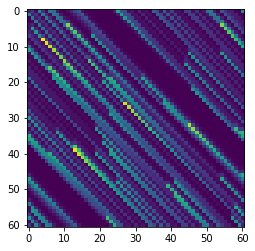
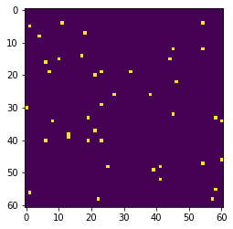
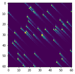
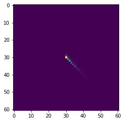
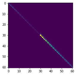
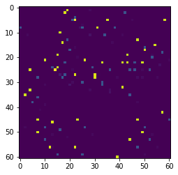
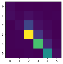
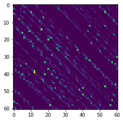
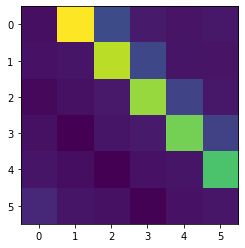
Figure 3: Sphere: $Y$, solved $X$, true $X$, solved $f$; previous $X$, previous $a$ as initialization, $a$ truth; $X$ solved by non-convex alternating formulation, $a$ solved by non-convex alternating formulation.

• $X$: $2-$D Bernoulli Gaussian IID of size $60\times 60$.

• $f^{\star}$: $1-$D filter $(1,-s,0)$ with $s=0.99$ centered and rotated by $45$ degree.

• $Y=a^{\star}*X$, where the filter inverse is defined by discrete Fourier transform on $60\times 60$ grid.

• $a^{\mbox{init}}$ = $f^{\mbox{init},-1}$, where $f^{\mbox{init}}$ is $1-$D filter $(1,-s_{\mbox{init}},0)$ with $s_{\mbox{init}}=0.8$ centered and rotated by $45$ degree.

• $X^{\mbox{init}}=a^{\mbox{init}}*X$ is the initial guess $a^{\mbox{init}}$ convolve with $X^{\star}$.

• $a^{\mbox{ncvx}}$ is the forward solved by alternating non-convex algorithm.

• $X^{\mbox{ncvx}}$ is the initial guess of $X$ solved by alternating non-convex algorithm.

• The plots in order, first row: $Y=a^{\star}*X^{\star}$, $X^{\mbox{cvx}}$, $X^{\star}$, $f^{\mbox{cvx}}=f^{\star}$.

• second row: $X^{\mbox{init}}$, $a^{\mbox{init}}$, $a^{\star}$;

• third row: $X^{\mbox{nc, init}}$, $a^{\mbox{nc,init}}$, $X^{\mbox{nc}}$, $a^{\mbox{nc}}$;

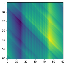
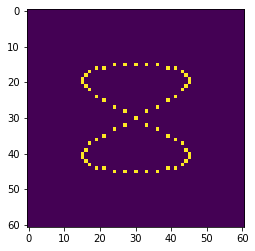
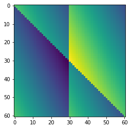
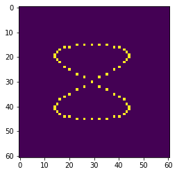
Figure 4: Sphere: $Y$, solved $X$, true $X$, solved $f$; previous $X$, previous $a$ as initialization, $a$ truth; $X$ solved by non-convex alternating formulation, $a$ solved by non-convex alternating formulation

• $X$: $2-$D centered shaped $8$ with frame size $15$ on size $60\times 60$ grid.

• $f^{\star}$: convolution of two $1-$D filters: $(1,-s_{1},0)$ with $s_{1}=0.9995$ centered and rotated by $45$ degree and $(1,-s_{2},0)$ with $s_{2}=0.9995$ centered and rotated by $0$ degree.

• $Y=a^{\star}*X$, where the filter inverse is defined by discrete Fourier transform on $60\times 60$ grid.

• $a^{\mbox{nc}}$ is the forward solved by alternating non-convex algorithm.

• $X^{\mbox{nc}}$ is the initial guess of $X$ solved by alternating non-convex algorithm.

• The plots in order, first row: $Y=a^{\star}*X^{\star}$, $X^{\star}$, $f^{\star}$, $a^{\star}$.

• second row: $X^{\mbox{cvx}}$, $f^{\mbox{cvx}}$ ,$X^{\mbox{nc}}$, $a^{\mbox{nc}}$;

Figure 5: $Y$, solved $X$, true $X$, solved $f$; previous $X$, previous $a$ as initialization, $a$ truth; $X$ solved by non-convex alternating formulation, $a$ solved by non-convex alternating formulation.

• $X$: $2-$D centered shaped $8$ on size $60\times 60$ grid.

• $f^{\star}$: convolution of two $1-$D centered filters: $(1,-s_{1},0)$, $s_{1}=0.999$, rotated by $45$ degree, . $(1,-s_{1}2,0)$, $s_{2}=0.9$, rotated by $0$ degree.

• $Y=f^{\star,-1}*X$, where the filter inverse is defined by discrete Fourier transform on $60\times 60$ grid.

• $a^{\mbox{nc}}$ is the forward solved by alternating non-convex algorithm.

• $X^{\mbox{nc}}$ is the initial guess of $X$ solved by alternating non-convex algorithm.

• The plots in order, first row: $Y=a^{\star}*X^{\star}$, $X^{\star}$, $f^{\star}$, $a^{\star}$.

• second row: $X^{\mbox{cvx}}$, $f^{\mbox{cvx}}$ ,$X^{\mbox{nc}}$, $a^{\mbox{nc}}$;

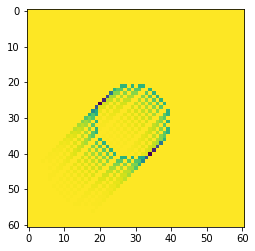
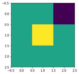
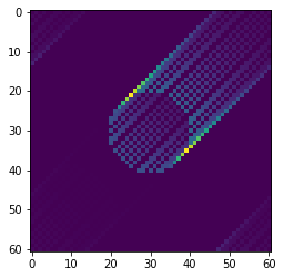
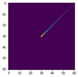
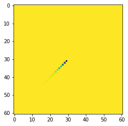
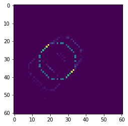
Figure 6: Sphere: $Y$, solved $X$, true $X$, solved $f$; previous $X$, previous $a$ as initialization, $a$ truth; $X$ solved by non-convex alternating formulation, $a$ solved by non-convex alternating formulation.

• $X$: $2-$D circle centered with radius $10$, on size $60\times 60$ grid.

• $f^{\star}$: $1-$D filter $(1,-s,0)$ centered and rotated by $45$ degree.

• $Y=f^{\star,-1}*X$, where the filter inverse is defined by discrete Fourier transform on $60\times 60$ grid.

• $a^{\mbox{ncvx}}$ is the forward solved by alternating non-convex algorithm.

• $X^{\mbox{ncvx}}$ is the initial guess of $X$ solved by alternating non-convex algorithm.

• The plots in order, first row: $Y=a^{\star}*X^{\star}$, $X^{\mbox{cvx}}$, $X^{\star}$, $f^{\mbox{cvx}}=f^{\star}$.

• second row: $X^{\mbox{init}}$, $a^{\mbox{init}}$, $a^{\star}$;

• third row: $X^{\mbox{nc}}$, $a^{\mbox{nc}}$, $f^{\mbox{nc}}$;

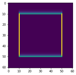
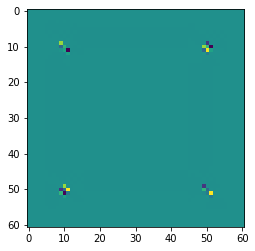
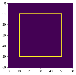
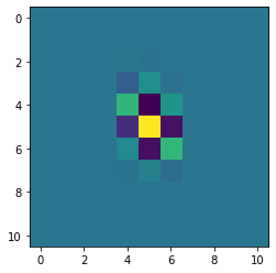
Figure 7: Failure mode-square, TV norm: $Y$, solved $X$, true $X$, solved $f$,

• $X$: $2-$D centered shaped square with frame size $40But$ on size $60\times 60$ grid.

• $f^{\star}$: convolution of two $1-$D filters: $(1,-s_{1},0)$ with $s_{1}=0.9995$ centered and rotated by $45$ degree and $(1,-s_{2},0)$ with $s_{2}=0.9995$ centered and rotated by $0$ degree.

• $Y=a^{\star}*X$, where the filter inverse is defined by discrete Fourier transform on $60\times 60$ grid.

• $a^{\mbox{nc}}$ is the forward solved by alternating non-convex algorithm.

• $X^{\mbox{nc}}$ is the initial guess of $X$ solved by alternating non-convex algorithm.

• The plots in order, first row: $Y=a^{\star}*X^{\star}$, $X^{\star}$, $f^{\star}$, $a^{\star}$.

• second row: $X^{\mbox{cvx}}$, $f^{\mbox{cvx}}$ ,$X^{\mbox{nc}}$, $a^{\mbox{nc}}$;

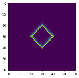
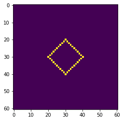
Figure 8: Failure mode-diamond, TV norm: $Y$, solved $X$, true $X$, solved $f$,

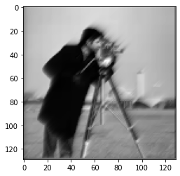
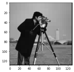
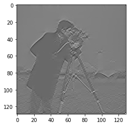
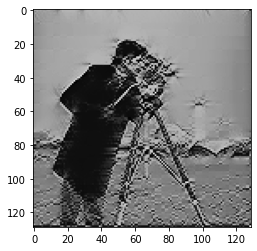
Figure 9: ‘Cameraman’, using TV norm and weighted Haar L1 norm ($5$ levels with weights $2^{j},j=0,\ldots 4$: $Y$, true $X$, TV norm solved $X$,Weighted Haar L1 norm solved $X$, true $f$, TV norm solved $f$,Weighted Haar L1 norm solved $f$ ,

• $X$: camera man figure, on size $128\times 128$ grid.

• $f^{\star}$: $1-$D filter $(1,-s,0)$ centered and rotated by $45$ degree.

• $Y=f^{\star,-1}*X$, where the filter inverse is defined by discrete Fourier transform on $60\times 60$ grid.

• $X^{\mbox{TV}}$ is the solution of convex problem with TV norm objective.

• $X^{\mbox{Haar}}$ is the solution of convex problem use weighted Haar L1 norm with $5$ levels as objective, where the weighted Haar L1 norm weights level $j$ coefficient by with weights $2^{j},j=0,\ldots 4$.

• The plots in order, first row: $Y=a^{\star}*X^{\star}$, $X^{\star}$,$X^{\mbox{TV}}$, $X^{\mbox{Haar}}$.

4 Techinical Overview and Proof Sketch for Phase Transition Theorems

4.1 Main Result $1$: Population (Large-$N$) Phase Transition

Sketch of proof ideas for Theorem 3

Here we highlight some of the key ideas in the proof:

• Change of variable. Rewrite the population version of our convex sparse blind deconvolution problem, with the population objective ${\mathbb{E}}\frac{1}{N}\|{\bf w}*Y\|_{\ell_{1}({\cal T})}={\mathbb{E}}|({\bf w}*Y)_{0}|={\mathbb{E}}|({\bf w}*{\bf a}*X)_{0}|={\mathbb{E}}_{X}|\langle X,({\bf w}*{\bf a})^{\dagger}\rangle|$ due to the ergodic property of stationary process and shift invariance, and $(\widetilde{{\bf a}}*{\bf w})_{0}=((\widetilde{{\bf a}}*{\bf a}^{-1})*({\bf a}*{\bf w}))_{0}=\langle(\widetilde{{\bf a}}*{\bf a}^{-1})^{\dagger},{\bf w}*{\bf a}\rangle$, the convex problem becomes

  $$\begin{array}[]{ll}\underset{{\bf w}}{\mbox{minimize}}&{\mathbb{E}}_{X}|\langle X,({\bf a}*{\bf w})^{\dagger}\rangle|\\ \mbox{subject to}&\langle\widetilde{{\bf a}}*{\bf a}^{-1},({\bf a}*{\bf w})^{\dagger}\rangle=1,\end{array}$$

  Let ${\bf v}$ denote the time reversed version of ${\bf a}*{\bf w}$: ${\bf v}:=({\bf a}*{\bf w})^{\dagger}$, and let $\widetilde{{\bf e}}:=\widetilde{{\bf a}}*{\bf a}^{-1}$, then by previous assumptions, $\widetilde{{\bf e}}(0)=1$, $\widetilde{{\bf e}}^{\prime}=\widetilde{{\bf e}}-{\bf e}_{0}$.

  Now we arrive at a simple and fundamental population convex problem:

  $$\begin{array}[]{ll}\underset{{\bf v}}{\mbox{minimize}}&{\mathbb{E}}_{X}|\langle X,{\bf v}\rangle|\\ \mbox{subject to}&\langle\widetilde{{\bf e}},{\bf v}\rangle=1.\end{array}$$

• Expectation using Gaussian. Since $X$ follows Bernoulli-Gaussian IID probability model $X_{t}=I_{t}G_{t}$, we nest the expectation over $I_{t}$ outside the expectation over Gaussian $G_{t}$, for which we use $E|N(0,1)|=\sqrt{\frac{2}{\pi}}$:

  $${\mathbb{E}}_{X}|\langle X,{\bf v}\rangle|={\mathbb{E}}_{I}{\mathbb{E}}_{G}{|\sum_{t\in{\mathbb{Z}}}I_{t}G_{t}{\bf v}(t)|}=\sqrt{\frac{2}{\pi}}\cdot{\mathbb{E}}_{I}\|{\bf v}\cdot I\|_{2}$$

• KKT condition for ${\bf e}_{0}$. Let ${\bf v}^{\star}$ denote the solution of the optimization problem:

  $$\begin{array}[]{ll}\underset{\psi}{\mbox{minimize}}&\sqrt{\frac{2}{\pi}}\cdot{\mathbb{E}}_{I}\|{\bf v}\cdot I\|_{2}\\ \mbox{subject to}&\langle\widetilde{{\bf e}},{\bf v}\rangle=1\end{array}$$

  To prove that ${\bf v}^{\star}={\bf e}_{0}$, i.e. ${\bf e}_{0}$ solves ($Q_{1}(\widetilde{{\bf e}})$), we calculate the directional finite difference at ${\bf e}_{0}$. Then ${\bf e}_{0}$ solves this convex problem if the directional finite difference at ${\bf v}={\bf e}_{0}$ is non-negative at every direction $\beta$ on unit sphere where $\widetilde{{\bf e}}^{T}\beta=0$:

  $${\mathbb{E}}\|({\bf e}_{0}+\beta)\cdot I\|_{2}-{\mathbb{E}}\|({\bf e}_{0})\cdot I\|_{2}\geq 0.$$

• Conditional expectation at one sparse element $X_{0}$. We decompose the objective into a sum of terms, conditioning on whether $I_{0}=1_{\{X_{0}\neq 0\}}$ is zero or not:

  $$\begin{array}[]{ll}{\mathbb{E}}\|({\bf e}_{0}+\beta)\cdot I\|_{2}-{\mathbb{E}}\|({\bf e}(0))\cdot I\|_{2}&=p(1+\beta_{0})+(1-p)\nabla_{\beta}{{\mathbb{E}}_{I}[\|({\bf e}_{0}+\beta)^{\prime}\|_{\ell_{2}(I-\{0\})}\mid I_{0}=0]}-p\\ &=p\beta_{0}+(1-p){\mathbb{E}}_{I^{\prime}}[\|\beta^{\prime}\|_{\ell_{2}(I^{\prime})}].\end{array}$$

  This will be non-negative in case either $\beta(0)>0$, or else $\beta(0)<0$ but

  $$\frac{p}{1-p}\leq\frac{{\mathbb{E}}_{I^{\prime}}\|\beta^{\prime}\|_{\ell_{2}(I^{\prime})}}{|\beta_{0}|}$$

  for all $\beta$ that satisfy $\widetilde{{\bf e}}^{T}\beta=0$.

• Reduction to $val(Q_{1}(\widetilde{{\bf e}}^{\prime})).$ We normalize the direction sequence $\beta$ so that $\beta(0)=-1$; using $\tilde{e}(0)=1$, we obtain a lowerbound:

  $$\inf_{\beta(0)=-1,\langle\widetilde{{\bf e}},\beta\rangle=0}{\mathbb{E}}_{I^{\prime}}\|\beta^{\prime}\|_{\ell_{2}(I^{\prime})}=\inf_{\beta(0)=-1,\beta(0)\tilde{e}(0)-\langle\widetilde{{\bf e}}^{\prime},\beta^{\prime}\rangle=0}{\mathbb{E}}_{I^{\prime}}\|\beta^{\prime}\|_{\ell_{2}(I^{\prime})}=\inf_{\langle\widetilde{{\bf e}}^{\prime},\beta^{\prime}\rangle=1}{\mathbb{E}}_{I^{\prime}}\|\beta^{\prime}\|_{\ell_{2}(I^{\prime})}=val(Q_{1}(\widetilde{{\bf e}}^{\prime}))$$

  Here $Q_{1}(\widetilde{{\bf e}}^{\prime})$ is the optimization problem:

  $$\begin{array}[]{ll}\underset{\beta\in l_{1}({\mathbb{Z}})}{\mbox{minimize}}&{\mathbb{E}}_{I^{\prime}}\|\beta^{\prime}\|_{\ell_{2}(I^{\prime})}\\ \mbox{subject to}&\langle\widetilde{{\bf e}}^{\prime},\beta^{\prime}\rangle=1\end{array}$$

• The explicit phase transition condition with upper and lower bound. We have shown the existence of $p^{\star}$ so that for all $p<p^{\star}$, the KKT condition is satisfied. And we have represented $p^{\star}$ as the optimal value of a derived optimization problem $val(Q_{1}(\widetilde{{\bf e}}^{\prime}))$. The following lemma finds simple upper and lower bounds for $p^{\star}=val(Q_{1}(\widetilde{{\bf e}}^{\prime}))$.

  Lemma 4.1 (Explicit phase transition condition with upper and lower bound).

  The threshold $p^{\star}$ determined by

  $$\frac{p}{1-p}=val(Q_{1}(\widetilde{{\bf e}}^{\prime})).$$

  obeys an upper bound and lower

  $$\frac{p}{\|\widetilde{{\bf e}}^{\prime}\|_{\infty}}\geq val(Q_{1}(\widetilde{{\bf e}}^{\prime}))\geq{\mathbb{E}}_{I}\|\widetilde{{\bf e}}^{\prime}\cdot I\|_{2}^{-1}$$

  where $\|\widetilde{{\bf e}}^{\prime}\|_{\infty}=\frac{|\widetilde{{\bf e}}|_{(2)}}{|\widetilde{{\bf e}}|_{(1)}}$. Additionally, the upper bound is sharp if and only if

  $$\frac{p}{1-p}\leq val(Q_{1}(\frac{\widetilde{{\bf e}}^{\prime}}{\|\widetilde{{\bf e}}^{\prime}\|_{\infty}}))=val(Q_{1}(\widetilde{{\bf e}}^{\prime\prime}))/\|\widetilde{{\bf e}}^{\prime}\|_{\infty}$$

  therefore, the upper bound holds with equality

  $$p^{\star}=1-\frac{|\widetilde{{\bf e}}|_{(2)}}{|\widetilde{{\bf e}}|_{(1)}}$$

  if

  $$p\leq 1-\frac{|\widetilde{{\bf e}}|_{(3)}}{|\widetilde{{\bf e}}|_{(2)}}$$

  Therefore, if

  $$\frac{|\widetilde{{\bf e}}|_{(3)}}{|\widetilde{{\bf e}}|_{(2)}}\leq\frac{|\widetilde{{\bf e}}|_{(2)}}{|\widetilde{{\bf e}}|_{(1)}}$$

  then

  $$p^{\star}=1-\frac{|\widetilde{{\bf e}}|_{(2)}}{|\widetilde{{\bf e}}|_{(1)}}.$$

  The above narrative gives a sketch of our result and its proof. The upper bound $1-\frac{|\widetilde{{\bf e}}|_{(2)}}{|\widetilde{{\bf e}}|_{(1)}}$ of $p^{\star}$ generalized the previous special case of exponential decay filter in theorem 1 with $p^{\star}=1-|s|$.

• Lemma 4.2 (Geometric lower bound $val(Q_{1}(\widetilde{{\bf e}}^{\prime}))$ for the phase transition condition).

  $$val(Q_{1}(\widetilde{{\bf e}}^{\prime}))\geq p\cot\angle(\widetilde{{\bf e}},{\bf e}_{0})$$

  where

  $$\cot\angle(\widetilde{{\bf e}},{\bf e}_{0})=\frac{1}{\|\widetilde{{\bf e}}^{\prime}\|_{2}}$$

• Using the technical background provided in theorem 9, we can further provide a tighter upper bound to compute phase transition $p^{\star}$.

  4.2 Technical Tools: Landscape of Expected Homogeneous Function over Bernoulli Support on Sphere

  Let

  $$V_{k}({\bf u}):=\frac{{\mathbb{E}}_{J}\|{\bf u}\cdot J\|_{2}^{k}}{\|{\bf u}\|^{k}_{2}}$$

  where ${\bf u}\in{\mathbb{R}}^{N}$, $J$ is a Bernoulli sequence indexed from $1$ to $N$.

  Expectation $V_{1}({\bf u}):={\mathbb{E}}_{J}\|{\bf u}\cdot J\|_{2}^{1}$ on sphere.

  Theorem 9.

  Let ${\bf u}\in{\mathbb{R}}^{N}$, then

  $$p\leq V_{1}({\bf u})\leq V_{1}(\frac{\sum_{j\in[N]}\pm{\bf e}_{j}}{\sqrt{N}})\leq\sqrt{p}.$$

  the lower bound is approached by on-sparse vectors ${\bf u}\in\{\pm{\bf e}_{i},i\in[N]\}$, and the upper bound is approached by ${\bf u}\in\{\frac{1}{\sqrt{N}}\sum_{j\in[N]}\pm{\bf e}_{j}\}$.

  Furthermore, all the stationary points of $V_{1}({\bf u})$ are $\{\frac{\sum_{i\in J}\pm{\bf e}_{i}}{\sqrt{N_{J}}}\}$ for different support $J\subset{\cal T}$, where $\{\pm{\bf e}_{i},i\in[N]\}$ are the global minimizers, and $\{\frac{1}{\sqrt{N}}\sum_{j\in[N]}\pm{\bf e}_{j}\}$ are the global maximizers. And for $J$ with $1<N_{J}<N$, $\{\frac{\sum_{i\in J}\pm{\bf e}_{i}}{\sqrt{N_{J}}}\}$ are saddle points with value

  $$V_{1}(\frac{\sum_{i\in J}\pm{\bf e}_{i}}{\sqrt{N_{J}}})={\mathbb{E}}_{I}\sqrt{\frac{\sum_{i\in J}1_{I_{i}}}{N_{J}}}=\sum_{j=0}^{N_{J}}(1-p)^{N_{J}-j}p^{j}{N_{J}\choose j}\sqrt{\frac{j}{N_{J}}}.$$

  To support geometric intuition, Figure 10 visualizes $V_{1}$ on the $2-$dimensional sphere.

  

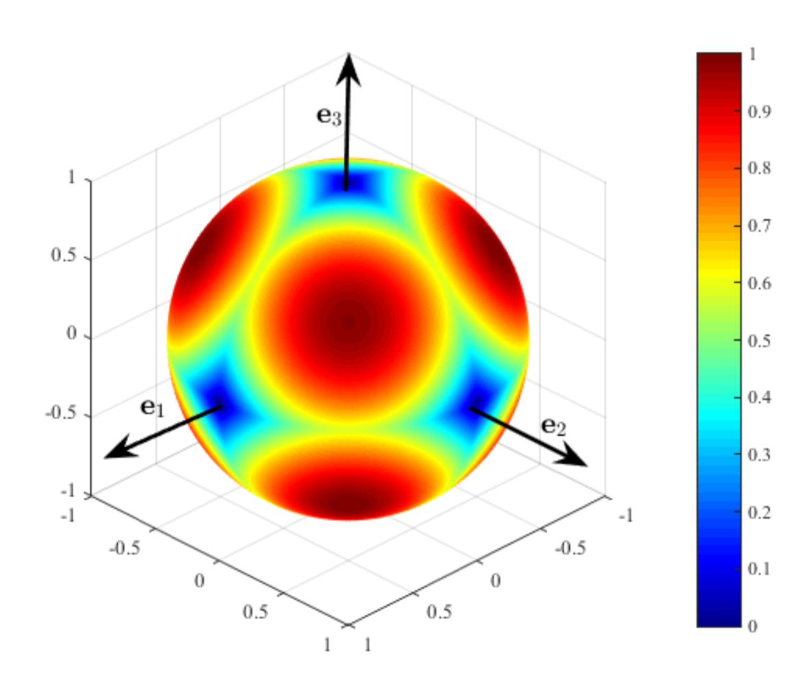
  Figure 10: The value of $V_{1}$ on a two-dimensional sphere in ${\mathbb{R}}^{3}$, normalized by the affine transform to send the value in $[0,1].$

  Expectation $V_{2k}({\bf u}):={\mathbb{E}}_{J}\|{\bf u}\cdot J\|_{2}^{2k}$ on sphere.

  Theorem 10.

  For $k\geq 2$, let ${\bf u}$ denote a vector in ${\mathbb{R}}^{N}$, then

  $$p^{k}\leq V_{2k}(\frac{\sum_{j\in[N]}\pm{\bf e}_{j}}{\sqrt{N}})\leq V_{2k}({\bf u})\leq p.$$

  the upper bound is approached by one-sparse vectors ${\bf u}\in\{\pm{\bf e}_{i},i\in[N]\}$, and the lower bound is approached by ${\bf u}\in\{\frac{1}{\sqrt{N}}\sum_{j\in[N]}\pm{\bf e}_{j}\}$.

  Furthermore, all the stationary points of $V_{2k}(\psi)$ are $\{\frac{\sum_{i\in J}\pm{\bf e}_{i}}{\sqrt{N_{J}}}\}$ for different support $J\subset{\cal T}$, where $\{\pm{\bf e}_{i},i\in[N]\}$ are the set of global maximizers, and $\{\frac{1}{\sqrt{N}}\sum_{j\in[N]}\pm{\bf e}_{j}\}$ are the set of all the global minimizers. And for $J$ with $1<N_{J}<N$, $\{\frac{\sum_{i\in J}\pm{\bf e}_{i}}{\sqrt{N_{J}}}\}$ are saddle points with value

  $$V_{2k}(\frac{\sum_{i\in J}\pm{\bf e}_{i}}{\sqrt{N_{J}}})={\mathbb{E}}_{J}(\frac{\sum_{i\in J}1_{I_{i}}}{N_{J}})^{k}=\sum_{j=0}^{N_{J}}(1-p)^{N_{J}-j}p^{j}{N_{J}\choose j}(\frac{j}{N_{J}})^{k}.$$

  Expectation $V_{-1}({\bf u}):={\mathbb{E}}_{J}\|{\bf u}\cdot J\|_{2}^{-1}$ on sphere.

  Theorem 11.

  $$V_{-1}({\bf u})\geq p^{-1/2}.$$ (8)

  4.3 Exact representation of $val(Q_{1})$

  Exact representation from support analysis

  Let $|\widetilde{{\bf e}}|$ be the entry-wise absolute value of $\widetilde{{\bf e}}$. We can rank the entries of $|\widetilde{{\bf e}}|$ to be $|\widetilde{{\bf e}}|_{(1)},|\widetilde{{\bf e}}|_{(2)},|\widetilde{{\bf e}}|_{(3)},\ldots$, then the entries of $\widetilde{{\bf e}}^{\prime}$ will be ranked as $|\widetilde{{\bf e}}|_{(2)},|\widetilde{{\bf e}}|_{(3)},\ldots$. By scaling we have $|\widetilde{{\bf e}}|_{(1)}=1$. We define $\widetilde{{\bf e}}_{S_{m}}$ as the vector that only keep the entries $\widetilde{{\bf e}}_{(2)},\widetilde{{\bf e}}_{(3)},\ldots,\widetilde{{\bf e}}_{(m+1)}$ of $\widetilde{{\bf e}}$, and send the rest of entries to zero.

  Lemma 4.3 (Exact representation of $val(Q_{1}(\widetilde{{\bf e}}^{\prime}))$ via support decomposition and $V_{1}$ function).

  $$val(Q_{1}(\widetilde{{\bf e}}^{\prime}))=\inf_{m\in\{1,2,\ldots,n_{e}-1\}}val(Q_{1}^{S_{m}})$$

Proof: Assume that $\widetilde{{\bf e}}$ has $n_{e}$ non-zero entry on support $S_{\widetilde{{\bf e}}}$, we can rank the absolute value of entries of $\widetilde{{\bf e}}$ to be $|\widetilde{{\bf e}}|_{(1)},|\widetilde{{\bf e}}|_{(2)},|\widetilde{{\bf e}}|_{(3)},\ldots,|\widetilde{{\bf e}}|_{(n_{e})}$, then the entries of $\widetilde{{\bf e}}^{\prime}$ will be ranked as $|\widetilde{{\bf e}}|_{(2)},|\widetilde{{\bf e}}|_{(3)},\ldots,|\widetilde{{\bf e}}|_{(n_{e})}$.

We know the optimal solution of $(\beta^{\prime})^{\star}$ of $\inf_{\langle\widetilde{{\bf e}}^{\prime},\beta^{\prime}\rangle=1}{\mathbb{E}}_{I^{\prime}}\|\beta^{\prime}\|_{\ell_{2}(I^{\prime})}$ must have support $S_{\beta^{\star}}$ that satisfy $S_{\star}\subset S_{\widetilde{{\bf e}}^{\prime}}$. From the symmetry of objective, we know if $(\beta^{\prime})^{\star}$ is $m$ sparse, then $m\leq n_{e}-1$ and, its support must be on the top $m$ entries $|\widetilde{{\bf e}}|_{(2)},|\widetilde{{\bf e}}|_{(3)},\ldots,|\widetilde{{\bf e}}|_{(m+1)}$, we call this support $S_{m}$, and we know the corresponding entries of $(\beta^{\prime})^{\star}$ would have the same sign as entries of $\widetilde{{\bf e}}$.

We can define the $m$ sparse optimization problem for a random support function on the subset of $S_{m}$: $J_{m}\subset S_{m}$. Let $\beta$ be supported on $S_{m}$ and each entry positive, then

$$val(Q_{1}^{S_{m}}):=\inf_{\beta:\sum_{j=1}^{m}|\widetilde{{\bf e}}|_{(j+1)}\beta_{j}=1,\beta_{j}>0}{\mathbb{E}}_{J_{m}}\|\beta\cdot J_{m}\|_{2}$$

The linear equality constraint comes from

$$\langle|\widetilde{{\bf e}}^{\prime}_{S_{m}}|,\beta^{\prime}\rangle=\sum_{j=1}^{m}|\widetilde{{\bf e}}|_{(j+1)}\beta_{j}=1$$

Then by breaking the case to find minimum over at most $n_{e}-1$ non-zero entries to the minimum of the cases to find minimum over exactly $m$ non-zero entries, and also use sign symmetry, we have

$$val(Q_{1}(\widetilde{{\bf e}}^{\prime}))=\inf_{m\in\{1,2,\ldots,n_{e}-1\}}val(Q_{1}^{S_{m}})$$

Tighter decomposition on $val(Q_{1})$

Now we can prove a more refine upper bound:

Lemma 4.4 (Tighter upper bound on $val(Q_{1})$).

$$val(Q_{1}(\widetilde{{\bf e}}^{\prime}))=\inf_{m\in\{1,2,\ldots,n_{e}-1\}}val(Q_{1}^{S_{m}})=\inf_{m\in\{1,2,\ldots,n_{e}-1\}}[V_{1}(\widetilde{{\bf e}}^{\prime}_{S_{m}})\cot\angle(\widetilde{{\bf e}}_{S_{m}},{\bf e}_{0})]$$

where $V_{1}$ function takes value in $[p,\sqrt{p})$.

More specifically, let the unit vector along the direction of $|\widetilde{{\bf e}}^{\prime}_{S_{m}}|$ be

$$u^{m}=|\widetilde{{\bf e}}^{\prime}_{S_{m}}|/\|\widetilde{{\bf e}}^{\prime}_{S_{m}}\|_{2}$$

$$val(Q_{1}^{S_{m}}) = \cot\angle(\widetilde{{\bf e}}_{S_{m}},{\bf e}_{0})V_{1}(|\widetilde{{\bf e}}^{\prime}_{S_{m}}|)C(u^{m})$$

where

$$C(u^{m}):=\frac{1}{V_{1}(u^{m})}\inf_{\beta^{m}:\beta^{m}_{j}>0}\frac{V_{1}(\beta^{m})}{\cos\angle(\beta^{m},u^{m})}=\frac{1}{E_{J_{m}}\|u^{m}\cdot J_{m}\|_{2}}\inf_{\beta^{m}:\beta^{m}_{j}>0}\frac{E_{J_{m}}\|\beta^{m}\cdot J_{m}\|_{2}}{\langle\beta^{m},u^{m}\rangle}$$

And we can prove that

$$C(u^{m})=1$$

Proof of lemma 4.3.

From

$$val(Q_{1}^{S_{m}}):=\inf_{\beta:\sum_{j=1}^{m}|\widetilde{{\bf e}}|_{(j+1)}\beta_{j}=1,\beta_{j}>0}{\mathbb{E}}_{J_{m}}\|\beta\cdot J_{m}\|_{2}$$

For a fixed $m$, after re-ranking the entries by absolute value, let $S_{m}$ be the support so that only the top $m$ entries $|\widetilde{{\bf e}}|_{(2)},|\widetilde{{\bf e}}|_{(3)},\ldots,|\widetilde{{\bf e}}|_{(m+1)}$ are non-zero, let

$$|\widetilde{{\bf e}}^{\prime}_{S_{m}}|=(0,|\widetilde{{\bf e}}|_{(2)},|\widetilde{{\bf e}}|_{(3)},\ldots,|\widetilde{{\bf e}}|_{(m+1)},0,\ldots,0)$$

$$\|\widetilde{{\bf e}}^{\prime}_{S_{m}}\|_{2}^{2}=|\widetilde{{\bf e}}|^{2}_{(2)}+|\widetilde{{\bf e}}|^{2}_{(3)}+\ldots+|\widetilde{{\bf e}}|^{2}_{(m+1)}$$

let the unit vector along the direction of $|\widetilde{{\bf e}}^{\prime}_{S_{m}}|$ be

$$u^{m}=|\widetilde{{\bf e}}^{\prime}_{S_{m}}|/\|\widetilde{{\bf e}}^{\prime}_{S_{m}}\|_{2}$$

so that $u^{m}_{j}>0$, $j\in S_{m}$. then

$$val(Q_{1}^{S_{m}}):=\frac{1}{\|\widetilde{{\bf e}}^{\prime}_{S_{m}}\|_{2}}\inf_{\beta:\beta_{j}>0}\{{\mathbb{E}}_{J_{m}}\|(\beta/\|\beta\|_{2})\cdot J_{m}\|_{2}\cdot\frac{1}{\sum_{j=1}^{m}u^{m}_{j}\frac{\beta_{j}}{\|\beta\|_{2}}}\}$$

From previous definition, since $\beta$ is supported on $S_{m}$, we denote it as $\beta^{m}$, then

$$V_{1}(\beta^{m})={\mathbb{E}}_{J_{m}}\|(\beta/\|\beta\|_{2})\cdot J_{m}\|_{2},$$

$$V_{1}(\widetilde{{\bf e}}^{\prime}_{S_{m}})=V_{1}(|\widetilde{{\bf e}}^{\prime}_{S_{m}}|)=V_{1}(u^{m}).$$

Geometrically,

$$\cos\angle(\beta^{m},u^{m})=\sum_{j=1}^{m}u^{m}_{j}\frac{\beta_{j}}{\|\beta\|_{2}}$$

$$\cot\angle(\widetilde{{\bf e}}_{S_{m}},{\bf e}_{0})=\frac{1}{\|\widetilde{{\bf e}}^{\prime}_{S_{m}}\|_{2}}$$

$$val(Q_{1}^{S_{m}})=\cot\angle(\widetilde{{\bf e}}_{S_{m}},{\bf e}_{0})\inf_{\beta:\beta_{j}>0}\{V_{1}(\beta^{m})\frac{1}{\cos\angle(\beta^{m},u^{m})}\}$$

Since $\beta^{m}=u^{m}$ is a feasible point of the linear equality constraint

$$\langle|\widetilde{{\bf e}}^{\prime}_{S_{m}}|,\beta^{\prime}\rangle=\sum_{j=1}^{m}|\widetilde{{\bf e}}|_{(j+1)}\beta_{j}=1,$$

we have an upper bound

$$val(Q_{1}^{S_{m}})\leq\cot\angle(\widetilde{{\bf e}}_{S_{m}},{\bf e}_{0})V_{1}(\widetilde{{\bf e}}^{\prime}_{S_{m}})$$

On the other hand,

$$val(Q_{1}^{S_{m}}) = \cot\angle(\widetilde{{\bf e}}_{S_{m}},{\bf e}_{0})\inf_{\beta:\beta_{j}>0}V_{1}(\beta^{m})\cdot\frac{1}{\cos\angle(\beta^{m},u^{m})}$$

$$= \cot\angle(\widetilde{{\bf e}}_{S_{m}},{\bf e}_{0})V_{1}(|\widetilde{{\bf e}}^{\prime}_{S_{m}}|)\inf_{\beta:\beta_{j}>0}\frac{V_{1}(\beta^{m})}{V_{1}(u^{m})}\cdot\frac{1}{\cos\angle(\beta^{m},u^{m})}$$

The lower bound is given by finding the lower bound of

$$C(u^{m}):=\frac{1}{V_{1}(u^{m})}\inf_{\beta^{m}:\beta^{m}_{j}>0}\frac{V_{1}(\beta^{m})}{\cos\angle(\beta^{m},u^{m})}=\frac{1}{E_{J_{m}}\|u^{m}\cdot J_{m}\|_{2}}\inf_{\beta^{m}:\beta^{m}_{j}>0}\frac{E_{J_{m}}\|\beta^{m}\cdot J_{m}\|_{2}}{\langle\beta^{m},u^{m}\rangle}$$

First, we know upper bound $C(u^{m})\leq 1$ by plug in $\beta^{m}=u^{m}$ as feasible point.

This value $C(u^{m})$ can be restricted to the $m$-dimensional subspace supported on $S_{m}$, therefore its value is independent of ambient space dimension, only dependent on the non-zero entries of $u^{m}$, without loss of generosity we only need to consider the case when $u^{m}$ is a $m$-dimensional dense vector lie on the first quadrant (all positive non-zero entries) of the unit sphere.

If $u^{m}$ approaches one-sparse point by taking the rest of coordinate close to zero, then $\beta^{m}$ should equal $u^{m}$.

On the other extreme, if $u^{m}$ is has $m$ equal entries $\frac{1}{\sqrt{m}}$, via numerical simulation we could check that

$$C(u^{m})=1$$

We conjecture that $C(u^{m})=1$.We only need to prove $C(u^{m})\geq 1$. To prove the lower bound, we only need to show that, on positive quadrant of $m$-dimensional unit sphere, the function

$$R_{u^{m}}(\beta^{m})=\frac{1}{E_{J_{m}}\|u^{m}\cdot J_{m}\|_{2}}\frac{E_{J_{m}}\|\beta^{m}\cdot J_{m}\|_{2}}{\langle\beta^{m},u^{m}\rangle}\geq 1$$

and takes minimum value $1$ at $\beta^{m}=u^{m}$.

In general, by symmetry, expect our guess $\beta^{m}=u^{m}$, for any $u^{m}$ on we could infer that the $2$ other types of points to check on positive quadrant of unit sphere are $\beta^{m}=(0,\sqrt{1-\epsilon^{2}},\sqrt{\epsilon},0\ldots,0)$ and $\beta^{m}=(\frac{1}{\sqrt{m}},\ldots,\frac{1}{\sqrt{m}}).$

First , for $\beta^{m}=(\frac{1}{\sqrt{m}},\ldots,\frac{1}{\sqrt{m}})$, then $\langle\beta^{m},u^{m}\rangle=\frac{1}{\sqrt{m}}1^{T}u^{m}\leq 1$ by Cauchy inequality, we have

$$R_{u^{m}}(\beta^{m})=\frac{1}{E_{J_{m}}\|u^{m}\cdot J_{m}\|_{2}}\frac{E_{J_{m}}\|\beta^{m}\cdot J_{m}\|_{2}}{\langle\beta^{m},u^{m}\rangle}\geq\frac{E_{J_{m}}\|(\frac{1}{\sqrt{m}},\ldots,\frac{1}{\sqrt{m}})\cdot J_{m}\|_{2}}{E_{J_{m}}\|u^{m}\cdot J_{m}\|_{2}}\geq 1$$

The last inequality comes from the saddle point property of $V_{1}$ at point $(\frac{1}{\sqrt{m}},\ldots,\frac{1}{\sqrt{m}})$. since $V_{1}((\frac{1}{\sqrt{m}},\ldots,\frac{1}{\sqrt{m}}))=\sum_{j=0}^{m}(1-p)^{m-j}p^{j}{m\choose j}\sqrt{\frac{j}{m}}=\sqrt{p}-\sum_{j=m+1}^{\infty}(1-p)^{m-j}p^{j}{m\choose j}\sqrt{\frac{j}{m}}\in[p,\sqrt{p}).$

Second, for $\beta^{m}=(0,\sqrt{1-\epsilon^{2}},\sqrt{\epsilon},0\ldots,0)$, if $\beta^{m}$ approaches one-sparse point by taking the rest of coordinate close to zero, by continuity of function $R_{u^{m}}(\beta^{m})$, we can consider the limit point on the boundary $\beta^{m}=(0,1,0,0\ldots,0)$, then

$$R_{u^{m}}(\beta^{m})=\frac{1}{E_{J_{m}}\|u^{m}\cdot J_{m}\|_{2}}\frac{E_{J_{m}}\|\beta^{m}\cdot J_{m}\|_{2}}{\langle\beta^{m},u^{m}\rangle}\geq\frac{p\|u^{m}\|^{2}_{2}}{E_{J_{m}}\|u^{m}\cdot J_{m}\|_{2}\|u^{m}\|_{\infty}}$$

We can first compute gradient of $R_{u^{m}}(\beta^{m})$, show that its directional gradient are all non-negative at $u^{m}$.

∎

4.4 Technical Tool: Relation between Finite Difference of Objective and Euclidean Distance

Bi-Lipschitzness of finite difference of objective

As an important proof tool, we study functional $B$ that allows us to bound the Euclidean distance $d_{2}(\psi,{\bf e}_{0}):=\|\psi-{\bf e}_{0}\|_{2}$ by the objective difference ${\mathbb{E}}_{I}\|\psi\cdot I\|_{2}-{\mathbb{E}}_{I}\|({\bf e}_{0})\cdot I\|_{2}$ :

$$B({\bf e}_{0},\phi):=\frac{{\mathbb{E}}_{I}\|({\bf e}_{0}+\phi)\cdot I\|_{2}-{\mathbb{E}}_{I}\|({\bf e}_{0})\cdot I\|_{2}}{\|\phi\|_{2}}$$

When we rescale $\phi$ to $\beta:=\frac{\phi}{\|\phi\|_{2}}$, we have

$$B({\bf e}_{0},t\beta)=\frac{{\mathbb{E}}_{I}\|({\bf e}_{0}+t\beta)\cdot I\|_{2}-{\mathbb{E}}_{I}\|({\bf e}_{0})\cdot I\|_{2}}{t}$$

From the definition of directional derivative,

$$\nabla_{\phi}{{\mathbb{E}}_{I}\|({\bf e}_{0}+\phi)\cdot I\|_{2}}\mid_{\phi=0}=\lim_{t\rightarrow 0^{+}}\frac{{\mathbb{E}}_{I}\|({\bf e}_{0}+t\beta)\cdot I\|_{2}-{\mathbb{E}}_{I}\|({\bf e}_{0})\cdot I\|_{2}}{t}=\lim_{t\rightarrow 0^{+}}B({\bf e}_{0},t\beta).$$

We have upper and lower bound on their difference. This upper and lower bound allows us to connect objective ${\mathbb{E}}_{I}\|\psi\cdot I\|_{2}$ and the $2-$norm of $\psi-{\bf e}_{0}$:

Theorem 12 (Bi-Lipschitzness of finite difference of objective near ${\bf e}_{0}$ for linear constraint).

We have upper and lower bound of $B({\bf e}_{0},\phi)$ :

$$0\leq B({\bf e}_{0},t\beta)-\lim_{t\rightarrow 0^{+}}B({\bf e}_{0},t\beta)\leq\frac{t}{2}p\Big{(}\beta_{0}^{2}+p(1-\beta_{0}^{2})\Big{)}\leq\frac{pt}{2}.$$

This leads to

$$0\leq B({\bf e}_{0},\phi)-\nabla_{\phi}{{\mathbb{E}}_{I}\|({\bf e}_{0}+\phi)\cdot I\|_{2}}\mid_{\phi=0}\leq\frac{p}{2}\|\phi\|_{2}.$$

Therefore, when $p<p^{\star}$, $\nabla_{\phi}{{\mathbb{E}}_{I}\|({\bf e}_{0}+\phi)\cdot I\|_{2}}\geq\epsilon(p,p^{\star})>0$, we have $B({\bf e}_{0},\phi)\geq\epsilon(p,p^{\star})>0$, which allows us to bound difference of objective by Euclidean distance . Reversely, $1/B({\bf e}_{0},\phi)\leq 1/\epsilon(p,p^{\star})$, which allows us to bound Euclidean distance by difference of objective.

5 Conclusion

In this paper, we proposed a novel convex optimization problem for sparse blind deconvolution problem based on $\ell^{1}$ minimization of inverse filter outputs:

$$\begin{array}[]{ll}\underset{{\bf w}\in l_{1}^{k}}{\mbox{minimize}}&\frac{1}{N}\|{\bf w}\star{\bf y}\|_{\ell_{1}^{N}}\\ \mbox{subject to}&\langle\widetilde{{\bf a}},{\bf w}^{\dagger}\rangle=1.\end{array}$$

Assuming the signal to be recovered is sufficiently sparse, the algorithm can convert a crude approximation to the filter into a high-accuracy recovery of the true filter.

We present four main results.

First, in a large-$N$ analysis where ${\bf x}$ is a realization of an IID Bernoulli-Gaussian signal with expected sparsity level $p$, we measure the approximation quality of $\widetilde{{\bf a}}$ by considering $\widetilde{{\bf e}}=\widetilde{{\bf a}}\star{\bf a}^{-1}$, which would be a Kronecker sequence if our approximation were perfect. Under the condition

$$\frac{|\widetilde{{\bf e}}|_{(2)}}{|\widetilde{{\bf e}}|_{(1)}}\leq 1-p,$$

we show that, in the large-$N$ limit, the $\ell^{1}$ minimizer ${\bf w}^{*}$ perfectly recovers ${\bf a}^{-1}$ to shift and scaling.

In words the less accurate the initial approximation $\widetilde{{\bf a}}\approx{\bf a}$, the greater we rely on sparsity of ${\bf x}$.

Second, we develop finite-$N$ guarantees of the form $N\geq O(k\log(k))$, for highly accurate reconstruction with high probability.

Third, we further show stable approximation when the true inverse filter is infinitely long (rather than length $k$), we show that the approximation error decrease exponentially as the approximation length growth.

Last, we extend our guarantees to the case where the observation contain stochastic or adversarial noise, we show that in both stochastic or adversarial noise cases, the approximation error growth linearly as a function of noise magnitude.

6 Supplementary: Landscape of Expected Homogeneous Function over Bernoulli Support on Sphere

In the following, we study the expected landscape for projection pursuit on sphere: $V_{1}$, $V_{2k}$, $V_{-1}$

First, we calculate ${\mathbb{E}}|\psi^{T}X|$ for $X_{t}$ IID sampled from Bernoulli Gaussian $pN(0,1)+(1-p)\delta_{0}.$ Let $X_{i}=B_{i}Z_{i}$ be IID Bernoulli Gaussian, where $B_{i}$ is sampled from Bernoulli with parameter $p$, $Z_{i}$ is sampled from $N(0,1)$. Let $I$ be the support where $B_{i}=1$.

From now on, we denote three equivalent notation, and interchange them for the convenience of each context:

$$\|\psi\|_{\ell_{2}(I)}=\|\psi_{I}\|_{2}=\|\psi\cdot I\|_{2}$$

6.1 Expectation of Inner Product for Sparse Signal

In the following, we study in detail the quantity

$$E{|\psi^{T}X|}=E{|\sum_{i}\psi_{i}X_{i}|}.$$

We know when $X_{i}$ have variance $\sigma^{2}$,

$$E(\sum_{i}\psi_{i}X_{i})^{2}=\sum_{i}\psi_{i}^{2}E(X_{i})^{2}=\sigma^{2}\|\psi\|_{2}^{2}.$$

The ratio indicates the sparsity level of the random variable $\sum_{i}\psi_{i}X_{i}$

$$\frac{E{|\sum_{i}\psi_{i}X_{i}|}}{\sqrt{E(\sum_{i}\psi_{i}X_{i})^{2}}}=\frac{E{|\sum_{i}\psi_{i}X_{i}|}}{\sigma^{2}\|\psi\|_{2}}$$

Now, we consider $E{|\sum_{i}\psi_{i}X_{i}|}$ in the general symmetric setting, where a lower bound can be derived.

Exact calculation for Bernoulli Gaussian

$${\mathbb{E}}_{X}{|\sum_{i}\psi_{i}X_{i}|}={\mathbb{E}}_{B}{\mathbb{E}}_{G}{|\sum_{i}\psi_{i}B_{i}G_{i}|}={\mathbb{E}}_{I}{\mathbb{E}}_{G}{|\sum_{i\in I}\psi_{i}G_{i}|}$$

Leveraging the fact that linear transforms of Gaussians are also Gaussian, we get

$${\mathbb{E}}_{G}{|\sum_{i\in I}\psi_{i}G_{i}|}=\sqrt{\frac{2}{\pi}}\cdot\|\psi_{I}\|_{2}.$$

Upper and lower bound for symmetric distribution

It is worth commenting that we could still calculate the upper and lower bound of ${\mathbb{E}}{|\psi^{T}X|}$ in terms of ${\mathbb{E}}_{I}\|\psi_{I}\|_{2}$ for $X_{t}$ IID sampled from any Bernoulli symmetric $pG+(1-p)\delta_{0}$, where $G$ is a symmetric distribution.

Lemma 6.1.

If we only know $\Xi_{i}$ are IID sampled from a symmetric distribution $F$ with unit variance, then we already have a lower bound,

$$1/\sqrt{2}\|a\|_{2}\leq{\mathbb{E}}|\sum_{i}a_{i}\Xi_{i}|\leq\|a\|_{2}.$$

Proof of Lemma 6.1.

The upper bound come from Cauchy inequality.

Now we derive the lower bound. We write $\Xi_{i}=\sigma_{i}|\Xi_{i}|$, where $s_{i}=\pm 1$ with equal probability since $\Xi_{i}$ are symmetric RV, and $\{s_{i},|\Xi_{i}|\}$ are all independent random variables. We could use Khintchine inequality,

$${\mathbb{E}}_{\Xi}|\sum_{i}a_{i}\Xi_{i}| = E_{|\Xi_{i}|}E_{s_{i}}|\sum_{i}a_{i}s_{i}|\Xi_{i}||$$

$$\geq 1/\sqrt{2}\sum_{i}a_{i}^{2}E_{|\Xi_{i}|}|\Xi_{i}|^{2}$$

$$= 1/\sqrt{2}\|a\|_{2}^{2}.$$

∎

Let $\psi_{I}=a$, we have a corollary for Bernoulli Symmetric case,

$${\mathbb{E}}_{I}\|\psi_{I}\|_{2}\geq{\mathbb{E}}_{X}{|\sum_{i}\psi_{i}X_{i}|}\geq\sqrt{\frac{1}{2}}\cdot{\mathbb{E}}_{I}\|\psi_{I}\|_{2}.$$

Theorem 13.

Let $X_{i}=B_{i}\Xi_{i}$ be IID, where $B_{i}$ is sampled from Bernoulli with parameter $p$, let $I$ be the support where $B_{i}=1$. And $\Xi_{i}$ is variance $1$, sampled from:

• $N(0,1)$

• general symmetric distribution with variance $1$.

Then

• (for Bernoulli Gaussian:)

  $${\mathbb{E}}_{X}{|\sum_{i}\psi_{i}X_{i}|}=\sqrt{\frac{2}{\pi}}\cdot{\mathbb{E}}_{I}\|\psi_{I}\|_{2}$$

• (for Bernoulli symmetric R.V. :)

  $${\mathbb{E}}_{I}\|\psi_{I}\|_{2}\geq{\mathbb{E}}_{X}{|\sum_{i}\psi_{i}X_{i}|}\geq\sqrt{\frac{1}{2}}\cdot{\mathbb{E}}_{I}\|\psi_{I}\|_{2}.$$

6.2 Expectation over Bernoulli Support

We previously considered the identity

$${\mathbb{E}}|\sum_{i\in{\cal T}}\psi_{i}X_{i}|=\sqrt{\frac{2}{\pi}}\cdot{\mathbb{E}}_{I}\|\psi\|_{\ell_{2}(I)},$$ (9)

where $X$ is a Bernoulli-Gaussian RV $BG(p;0,1)$, and where $I$ is a random subset of the domain ${\cal T}$ determined by Bernoulli-$p$ coin tossing.

Let $J\subset{\cal T}$ be the support of $X$, where $N:=|{\cal T}|$, $N_{J}:=|J|$. Let $\psi_{J}:=\psi\cdot 1_{J}$ denote the elementwise product of vector $\psi$ with the indicator vector of subset $J$. Then we can consider our problem on the space ${\cal T}$ by default, and rewrite for simplicity

$$\|\psi_{J}\|_{2}:=\|\psi_{J}\|_{\ell_{2}({\cal T})}=\|\psi\|_{\ell_{2}(J)}.$$

This leads us to consider the following ratio:

$$V^{J}_{k}(\psi):=\frac{\|\psi\|_{\ell_{2}(J)}^{k}}{\|\psi\|_{\ell_{2}({\cal T})}^{k}},$$

and its expectation over all Bernoulli random subset,

$$V_{k}(\psi):=\frac{{\mathbb{E}}_{I}\|\psi\|_{\ell_{2}(I)}^{k}}{\|\psi\|_{\ell_{2}({\cal T})}^{k}},$$

where $I$ is again a random subset. We remark that the lower bound of $V_{k}(\psi)$ is the optimal value of the optimization problem:

$$\min {\mathbb{E}}_{I}\|\psi_{I}\|^{k}_{2}$$

subject to $$\|\psi\|_{2}=1,$$

and the upper bound of $V_{k}(\psi)$ is the optimal value of the optimization problem

$$\max {\mathbb{E}}_{I}\|\psi_{I}\|^{k}_{2}$$

subject to $$\|\psi\|_{2}=1.$$

Lemma 6.2.

Let $\psi$ denote a vector in ${\mathbb{R}}^{N}$. For fixed support $J\subset[N]$ then for any $k\neq 0$, the deterministic quantity $V^{J}_{k}(\psi)$ satisfies:

$$0\leq V^{J}_{k}(\psi)\leq 1.$$

The upper bound is approached by the vectors $\psi\in\{\frac{1}{\sqrt{N}}\sum_{j\in J}\pm e_{j}\}$, where $\|\psi_{J}\|_{2}^{k}/\|\psi\|_{2}^{k}=1$, and the lower bound is approached by any $\psi$ that has all of its entries on $J$ to be zero.

Lemma 6.3.

Let $\psi$ denote a vector in ${\mathbb{R}}^{N}$.

$$V_{2}(\psi)=p.$$

Theorem 14.

Let $\psi$ denote a vector in ${\mathbb{R}}^{N}$, then

$$p\leq V_{1}(\psi)\leq V_{1}(\frac{\sum_{j\in[N]}\pm e_{j}}{\sqrt{N}})\leq\sqrt{p}.$$

the lower bound is approached by on-sparse vectors $\psi\in\{\pm e_{i},i\in[N]\}$, and the upper bound is approached by $\psi\in\{\frac{1}{\sqrt{N}}\sum_{j\in[N]}\pm e_{j}\}$.

Furthermore, all the stationary points of $V_{1}(\psi)$ are $\{\frac{\sum_{i\in J}\pm e_{i}}{\sqrt{N_{J}}}\}$ for different support $J\subset{\cal T}$, where $\{\pm e_{i},i\in[N]\}$ are the global minimizers, and $\{\frac{1}{\sqrt{N}}\sum_{j\in[N]}\pm e_{j}\}$ are the global maximizers. And for $J$ with $1<N_{J}<N$, $\{\frac{\sum_{i\in J}\pm e_{i}}{\sqrt{N_{J}}}\}$ are saddle points with value

$$V_{1}(\frac{\sum_{i\in J}\pm e_{i}}{\sqrt{N_{J}}})={\mathbb{E}}_{I}\sqrt{\frac{\sum_{i\in J}1_{I_{i}}}{N_{J}}}=\sum_{j=0}^{N_{J}}(1-p)^{N_{J}-j}p^{j}{N_{J}\choose j}\sqrt{\frac{j}{N_{J}}}.$$

Remark: Specifically,

$$V_{1}(e_{i})=p.$$

$$V_{1}(\frac{e_{i}+e_{j}}{\sqrt{2}})=p(\sqrt{2}+(1-\sqrt{2}p)).$$

Theorem 15.

For $k\geq 2$, let $\psi$ denote a vector in ${\mathbb{R}}^{N}$, then

$$p^{k}\leq V_{2k}(\frac{\sum_{j\in[N]}\pm e_{j}}{\sqrt{N}})\leq V_{2k}(\psi)\leq p.$$

the upper bound is approached by on-sparse vectors $\psi\in\{\pm e_{i},i\in[N]\}$, and the lower bound is approached by $\psi\in\{\frac{1}{\sqrt{N}}\sum_{j\in[N]}\pm e_{j}\}$.

Furthermore, all the stationary points of $V_{2k}(\psi)$ are $\{\frac{\sum_{i\in J}\pm e_{i}}{\sqrt{N_{J}}}\}$ for different support $J\subset{\cal T}$, where $\{\pm e_{i},i\in[N]\}$ are the set of global maximizers, and $\{\frac{1}{\sqrt{N}}\sum_{j\in[N]}\pm e_{j}\}$ are the set of all the global minimizers. And for $J$ with $1<N_{J}<N$, $\{\frac{\sum_{i\in J}\pm e_{i}}{\sqrt{N_{J}}}\}$ are saddle points with value

$$V_{2k}(\frac{\sum_{i\in J}\pm e_{i}}{\sqrt{N_{J}}})={\mathbb{E}}_{I}(\frac{\sum_{i\in J}1_{I_{i}}}{N_{J}})^{k}=\sum_{j=0}^{N_{J}}(1-p)^{N_{J}-j}p^{j}{N_{J}\choose j}(\frac{j}{N_{J}})^{k}.$$

6.3 Upper and Lower bound on Expectation of Norm over Bernoulli Support

Tight bound on $V_{1}$ and $V_{2k}$ using mean and variance of $\frac{\sum_{i\in J}1_{I_{i}}}{N_{J}}$

Now notice that

$$\frac{\sum_{i\in J}1_{I_{i}}}{N_{J}}$$

has mean $p$ and variance $\frac{p(1-p)}{N_{J}}$. We could define a zero mean unit variance random variable $g^{J}$ as a function of $\{1_{I_{i}}\mid i\in J\}$

$$g^{J}:=\left(\frac{\sum_{i\in J}1_{I_{i}}}{N_{J}}-p\right)/\left(\sqrt{\frac{p(1-p)}{N_{J}}}\right)$$

namely, ${\mathbb{E}}_{I}\left(g^{I}\right)=0,{\mathbb{E}}_{I}\left(g^{I}\right)^{2}=1$. then

$$\frac{\sum_{i\in J}1_{I_{i}}}{N_{J}}:=p+\sqrt{\frac{p(1-p)}{N_{J}}}g^{J}=p(1+\sqrt{\frac{1-p}{pN_{J}}}g^{J})$$

then

$${\mathbb{E}}_{I}\sqrt{\frac{\sum_{i\in J}1_{I_{i}}}{N_{J}}}={\mathbb{E}}_{I}\sqrt{p-\sqrt{\frac{p(1-p)}{N_{J}}}g^{I}}=\sqrt{p}{\mathbb{E}}_{I}\sqrt{1+\sqrt{\frac{1-p}{pN_{J}}}g^{I}}$$

$${\mathbb{E}}_{I}\left(\frac{\sum_{i\in J}1_{I_{i}}}{N_{J}}\right)^{k}=p^{k}{\mathbb{E}}_{I}\left({1+\sqrt{\frac{1-p}{pN_{J}}}g^{I}}\right)^{k}$$

Lemma 6.4.

For $0\leq x\leq 1,$

$$(1-x)^{1/2}=1-\sum_{\ell=0}^{\infty}\frac{2}{\ell+1}\binom{2\ell}{\ell}\left(\frac{x}{4}\right)^{\ell+1}$$ (10)

Lemma 6.5 (Taylor expansion for $V_{1}$).

Using Taylor expansion, asymptotically when $N_{J}\rightarrow\infty$,

$$\frac{1}{\sqrt{p}}{\mathbb{E}}_{I}\sqrt{\frac{\sum_{i\in J}1_{I_{i}}}{N_{J}}} = {\mathbb{E}}_{I}\left({1+\sqrt{\frac{1-p}{pN_{J}}}g^{I}}\right)^{1/2}$$

$$= 1-\sum_{\ell=0}^{\infty}\frac{2}{\ell+1}\binom{2\ell}{\ell}2^{-2(\ell+1)}\left(\sqrt{\frac{1-p}{pN_{J}}}\right)^{\ell+1}{\mathbb{E}}_{I}\left(g^{I}\right)^{\ell+1}$$

$$= 1-2^{-3}({\frac{1-p}{pN_{J}}})+O\left(({\frac{1-p}{pN_{J}}})^{2}\right).$$

Lemma 6.6 (Taylor expansion for $V_{2k}$).

Using Taylor expansion, asymptotically when $N_{J}\rightarrow\infty$,

$$\frac{1}{p^{k}}{\mathbb{E}}_{I}({\frac{\sum_{i\in J}1_{I_{i}}}{N_{J}}})^{k} = {\mathbb{E}}_{I}\left({1+\sqrt{\frac{1-p}{pN_{J}}}g^{I}}\right)^{k}$$

$$= 1+\sum_{\ell=1}^{k}\binom{k}{\ell}({\frac{1-p}{pN_{J}}})^{\ell/2}{\mathbb{E}}_{I}(g^{I})^{\ell}$$

$$= 1+\frac{k(k-1)}{2}({\frac{1-p}{pN_{J}}})+O\left(({\frac{1-p}{pN_{J}}})^{2}\right).$$

Therefore, we know what when $N_{J}>>1$, $V_{1}(\frac{\sum_{i\in J}1_{I_{i}}}{N_{J}})$ is close to its upper bound $\sqrt{p}$, and for $k\geq 2$, $V_{k}(\frac{\sum_{i\in J}1_{I_{i}}}{N_{J}})$ is close to its lower bound $p^{k}$. Namely

$${\mathbb{E}}_{I}\sqrt{\frac{\sum_{i\in J}1_{I_{i}}}{N_{J}}}\approx\sqrt{p},$$

$${\mathbb{E}}_{I}(\frac{\sum_{i\in J}1_{I_{i}}}{N_{J}})^{k}\approx p^{k}.$$

To gain geometric intuition, we visualize $V_{1}$ in $2-$dimensional sphere in figure 10.

Figure 11: The value of $V_{1}(\psi)$ for different $\psi$, $x-$axis is the sparsity parameter $p$, $y-$axis is $V_{1}(\psi)$.

Figure 12: The value of $V_{4}(\psi)$ for different $\psi$, $x-$axis is the sparsity parameter $p$, $y-$axis is $V_{4}(\psi)$.

Figure 13: The value of $V_{8}(\psi)$ for different $\psi$, $x-$axis is the sparsity parameter $p$, $y-$axis is $V_{8}(\psi)$.

6.4 Proofs of Upper and Lower Bounds

Proof of Theorem 9.

First, we show that the upper and lower bound value we give is achievable.

• When $\psi=e_{0}$,

  $${\mathbb{E}}_{I}\|(e_{0})_{I}\|_{2}=p\|(e_{0})\|_{2}+(1-p)\|0\|_{2}=p.$$

• When $\psi=\frac{1}{\sqrt{N}}\sum_{j\in[N]}\pm e_{j},$ then

  $$V_{1}(\psi)={\mathbb{E}}_{I}\sqrt{\frac{\sum_{i\in[N]}1_{I_{i}}}{N}}\leq\sqrt{{\mathbb{E}}_{I}\frac{\sum_{i\in[N]}1_{I_{i}}}{N}}=\sqrt{p}.$$

  The inequality comes from Jensen’s inequality, since square root function is concave.

• For fixed support $J$, when $\psi=\frac{1}{\sqrt{N_{J}}}\sum_{i\in J}e_{i},$ then $\|\psi_{J}\|_{2}/\|\psi\|_{2}=1.$ However, the expectation is going to be smaller for $p<1$.

  $$V_{1}(\psi)={\mathbb{E}}_{I}\sqrt{\frac{\sum_{i\in J}1_{I_{i}}}{N_{J}}}=\sum_{k=0}^{N_{J}}(1-p)^{N_{J}-k}p^{k}{N_{J}\choose k}\sqrt{\frac{k}{N_{J}}}.$$

This problem can be reformulated as projection pursuit with sphere constraint,

$$\min {\mathbb{E}}_{I}\|\psi_{I}\|_{2}$$

subject to $$\|\psi\|_{2}=1.$$

Then from [Bai et al., 2018] Proposition $3.3$, we get the result.

The main idea of the proof is to calculate the projected gradient for $q\in\{\frac{\sum_{i\in J}\pm e_{i}}{\sqrt{N_{J}}}\}$, when $N_{J}=M,$

$$e_{j}^{T}{\mathbb{E}}_{I}\partial\|(q)_{I}\|_{2}=q_{j}[\sum_{k=0}^{M}(1-p)^{M-k}p^{k}{M\choose k}\sqrt{\frac{k}{M}}],$$

therefore,

$${\mathbb{E}}_{I}\partial\|(q)_{I}\|_{2}=[\sum_{k=0}^{M}(1-p)^{M-k}p^{k}{M\choose k}\sqrt{\frac{k}{M}}]q,$$

so

$$(I-qq^{T}){\mathbb{E}}_{I}\partial\|q_{I}\|_{2}=[\sum_{k=0}^{M}(1-p)^{M-k}p^{k}{M\choose k}\sqrt{\frac{k}{M}}]q-[\sum_{k=0}^{M}(1-p)^{M-k}p^{k}{M\choose k}\sqrt{\frac{k}{M}}]q=0.$$

then $q\in\{\frac{\sum_{i\in J}\pm e_{i}}{\sqrt{N_{J}}}\}$ are stationary points.

The other direction (all other points are not stationary) is implied by (the proof of) Theorem $3.4$ in [Bai et al., 2018]. ∎

Proof of Lemma 6.4.

From generalized binomial theorem, we know that for $0\leq x\leq 1,$

$$(1-x)^{1/2}=\sum_{\ell=0}^{\infty}\binom{1/2}{\ell}(-x)^{\ell}.$$ (11)

$$\binom{1/2}{\ell} =\frac{\frac{1}{2}(\frac{1}{2}-1)(\frac{1}{2}-2)\cdots(\frac{1}{2}-\ell+1)}{\ell!}$$ (12)

$$=\frac{(-1)^{\ell-1}}{2^{\ell}\ell!}1\cdot 3\cdot 5\cdots(2\ell-3)$$ (13)

$$=\frac{(-1)^{\ell-1}}{2^{\ell}\ell!}\frac{(2\ell-2)!}{2^{\ell-1}(\ell-1)!}$$ (14)

$$=\frac{(-1)^{\ell-1}}{\ell 2^{2\ell-1}}\binom{2\ell-2}{\ell-1},$$ (15)

then

$$(1-x)^{1/2} =1-\sum_{\ell=1}^{\infty}\frac{2}{\ell}\binom{2\ell-2}{\ell-1}\left(\frac{x}{4}\right)^{\ell}$$ (16)

$$=1-\sum_{\ell=0}^{\infty}\frac{2}{\ell+1}\binom{2\ell}{\ell}\left(\frac{x}{4}\right)^{\ell+1}.$$ (17)

∎

Proof of Lemma 6.5.

$${\mathbb{E}}_{I}\sqrt{1-\sqrt{\frac{1-p}{pN_{J}}}g^{I}} = 1-\sum_{\ell=0}^{\infty}\frac{2}{\ell+1}\binom{2\ell}{\ell}2^{-2(\ell+1)}\left(\sqrt{\frac{1-p}{pN_{J}}}\right)^{\ell+1}{\mathbb{E}}_{I}\left(g^{I}\right)^{\ell+1}$$

$$= 1-2^{-3}({\frac{1-p}{pN_{J}}})-O(({\frac{1-p}{pN_{J}}})^{2})$$

Using the central limit theorem, when $N_{J}\rightarrow\infty$, we have normal approximation for $g^{J}$ so that

$$\frac{\sum_{i\in J}1_{I_{i}}}{N_{J}}\sim N(p,\sqrt{\frac{p(1-p)}{N_{J}}}),$$

then for $G\sim N(0,1),$ asymptotically when $N_{J}\rightarrow\infty$,

$${\mathbb{E}}_{I}\sqrt{\frac{\sum_{i\in J}1_{I_{i}}}{N_{J}}}\approx\sqrt{p}{\mathbb{E}}_{G}\sqrt{1-\sqrt{\frac{1-p}{pN_{J}}}G}=\sqrt{p}\left(1-2^{-3}(1-p)^{2}N_{J}^{-1}+O((1-p)^{4}N_{J}^{-2})\right),$$

where

$${\mathbb{E}}_{I}\sqrt{1-\sqrt{\frac{1-p}{pN_{J}}}g^{I}} \approx {\mathbb{E}}_{G}\sqrt{1-\sqrt{\frac{1-p}{pN_{J}}}G}$$

$$= 1-\sum_{\ell=0}^{\infty}\frac{2}{\ell+1}\binom{2\ell}{\ell}2^{-2(\ell+1)}\left(\sqrt{\frac{1-p}{pN_{J}}}\right)^{\ell+1}{\mathbb{E}}_{G}\left(G\right)^{\ell+1}$$

$$= 1-\sum_{\ell\mbox{ is odd}}^{\infty}\frac{2}{\ell+1}\binom{2\ell}{\ell}2^{-2(\ell+1)}\left(\sqrt{\frac{1-p}{pN_{J}}}\right)^{\ell+1}(\ell)!!$$

$$= 1-\sum_{s=1}^{\infty}\frac{1}{s}\binom{4s-2}{2s-1}2^{-4s}(2s-1)!!(p^{-1}-1)^{s}N_{J}^{-s}$$

$$= 1-\sum_{s=1}^{\infty}\frac{1}{s}\frac{(4s-2)!}{(2s-1)!(2s-1)!}2^{-4s}\frac{(2s-1)!}{2^{s-1}(s-1)!}(p^{-1}-1)^{s}N_{J}^{-s}$$

$$= 1-\sum_{s=1}^{\infty}\frac{(4s-2)!}{(2s-1)!(s)!}2^{-5s+1}(p^{-1}-1)^{s}N_{J}^{-s}.$$

∎

6.5 Bound on Harmonic Expectation

Bounds on $V_{-1}(\psi)=\frac{{\mathbb{E}}_{I}\|\psi\|^{-1}_{\ell_{2}(I)}}{\|\psi\|^{-1}_{\ell_{2}({\cal T})}}$

Lemma 6.7.

For $0\leq x\leq 1,$

$$(1-x)^{-1/2}=\sum_{\ell=0}^{\infty}\frac{1}{2^{2\ell}}\binom{2\ell}{\ell}\left(x\right)^{\ell}$$ (18)

Proof.

From generalized binomial theorem, we know that for $0\leq x\leq 1,$

$$(1-x)^{-1/2}=\sum_{\ell=0}^{\infty}\binom{-1/2}{\ell}(-x)^{\ell}$$ (19)

$$\binom{-1/2}{\ell}(-1)^{\ell} =\frac{-\frac{1}{2}(-\frac{1}{2}-1)(-\frac{1}{2}-2)\cdots(-\frac{1}{2}-\ell+1)}{\ell!}$$ (20)

$$=\frac{1}{2^{\ell}\ell!}1\cdot 3\cdot 5\cdots(2\ell-1)$$ (21)

$$=\frac{1}{2^{\ell}\ell!}\frac{(2\ell)!}{2^{\ell}(\ell)!}$$ (22)

$$=\frac{1}{2^{2\ell}}\binom{2\ell}{\ell}$$ (23)

∎

Theorem 16.

$$V_{-1}(\psi)=\frac{{\mathbb{E}}_{I}\|\psi\|^{-1}_{\ell_{2}(I)}}{\|\psi\|^{-1}_{\ell_{2}({\cal T})}}\geq p^{-1/2}\geq 1+\frac{1}{2}(1-p)\geq 1.$$ (24)

Proof.

For any fixed support $J\subset{\cal T},$

$$\frac{\|\psi\|^{-1}_{\ell_{2}(J)}}{\|\psi\|^{-1}_{\ell_{2}({\cal T})}}=\sqrt{\frac{\|\psi\|^{2}_{\ell_{2}({\cal T})}}{\|\psi\|^{2}_{\ell_{2}(J)}}}\geq 1.$$ (25)

Therefore,

$$\frac{{\mathbb{E}}_{I}\|\psi\|^{-1}_{\ell_{2}(I)}}{\|\psi\|^{-1}_{\ell_{2}({\cal T})}}\geq 1.$$ (26)

On the other hand, let

$${\mathbb{E}}_{I}(\frac{\|\psi\|_{\ell_{2}(I)}}{\|\psi\|_{\ell_{2}({\cal T})}})^{-1}={\mathbb{E}}_{I}(1-\frac{\|\psi\|^{2}_{\ell_{2}({\cal T}-I)}}{\|\psi\|^{2}_{\ell_{2}({\cal T})}})^{-1/2}.$$ (27)

For a fixed true subset $J\subset{\cal T}$ define the ratio $\rho_{{\cal T}-J}\equiv\frac{\|\psi\|^{2}_{\ell_{2}({\cal T}-J)}}{\|\psi\|^{2}_{\ell_{2}({\cal T})}}$; it obeys $0\leq\rho_{J}\leq 1$. Assume $\rho_{J}<1$

$$(1-\rho_{{\cal T}-J})^{-1/2}=\sum_{\ell=0}^{\infty}\frac{1}{2^{2\ell}}\binom{2\ell}{\ell}\left(\rho_{{\cal T}-J}\right)^{\ell}$$ (28)

Now with $J$ a random subset as earlier, we induce a random variable $\rho_{I}$.

$${\mathbb{E}}_{J}(1-\rho_{{\cal T}-J})^{-1/2}=\sum_{\ell=0}^{\infty}\frac{1}{2^{2\ell}}\binom{2\ell}{\ell}{\mathbb{E}}_{J}\left(\rho_{{\cal T}-J}\right)^{\ell}$$ (29)

We apply the bound on $V_{2\ell}$ for $\ell\geq 2$, where $p$ in the final formula is replaced by $1-p$.

We obtain for $\ell\geq 2$

$$(1-p)^{\ell}\leq{\mathbb{E}}_{J}\rho_{{\cal T}-J}^{\ell}\leq(1-p),$$

$${\mathbb{E}}_{J}(1-\rho_{{\cal T}-J})^{-1/2} =\sum_{\ell=0}^{\infty}\frac{1}{2^{2\ell}}\binom{2\ell}{\ell}{\mathbb{E}}_{J}\left(\rho_{{\cal T}-J}\right)^{\ell}$$ (30)

$$\geq\sum_{\ell=0}^{\infty}\frac{1}{2^{2\ell}}\binom{2\ell}{\ell}(1-p)^{\ell}$$ (31)

$$=(1-(1-p))^{-1/2}$$ (32)

$$=p^{-1/2}$$ (33)

$$\geq 1+\frac{1}{2}(1-p)$$ (34)

∎

7 Supplementary: Background for Convex Blind Deconvolution Problem

7.1 Technical Background: Wiener’s Lemma and Inverse Filter

Fourier transform and inverse filter

The discrete-time Fourier transform $\mathcal{F}$ is defined by $\mathcal{F}{\bf a}$ where

$$(\mathcal{F}{\bf a})(\omega):=\sum_{n=-\infty}^{\infty}a_{n}\,e^{2\pi in\omega},\quad\omega\in T=[-\frac{1}{2},\frac{1}{2}];$$

the inverse Fourier transform $\mathcal{F}^{-1}$ is defined by

$$(\mathcal{F}^{-1}f)(n)=\int_{-\frac{1}{2}}^{\frac{1}{2}}f(\omega)e^{-2\pi in\omega}d\omega,\quad n\in{\mathbb{Z}}.$$

Now, our condition on the filter ${\bf a}$ is:

$$a\in l_{1}({\mathbb{Z}}),(\mathcal{F}{\bf a})(\omega)\neq 0,\forall\omega\in T.$$

In the following theorem, we show that this condition would provide the existence of an inverse filter in $l_{1}({\mathbb{Z}})$.

First, we present the standard Wiener’s lemma.

Lemma 7.1.

Wiener’s lemma on periodic functions: Assume that a function $f$ on unit circle has an absolutely converging Fourier series, and $f(t)\neq 0$ for all $t\in T$, then $1/f$ also has an absolutely convergent Fourier series.

Then we can see clearly that the Fourier series version of the previous lemma would guarantee the existence of an inverse filter in $l_{1}({\mathbb{Z}})$.

Lemma 7.2.

Wiener’s lemma on $l_{1}({\mathbb{Z}})$ sequences : If ${\bf a}\in l_{1}({\mathbb{Z}}),(\mathcal{F}{\bf a})(\omega)\neq 0,\forall\omega\in T,$ we could define the inverse filter of ${\bf a}$ as ${\bf a}^{-1}:=\mathcal{F}^{-1}(\frac{1}{\mathcal{F}{\bf a}})$ so that ${\bf a}^{-1}*a={\bf e}_{0}.$ Here $e_{0}$ is the sequence with $1$ at $0$ coordinate and $0$ elsewhere. From Wiener’s lemma on $\mathcal{F}{\bf a}$, ${\bf a}^{-1}\in l_{1}({\mathbb{Z}})$ .

7.2 Change of Variable and Reduction to Projection Pursuit

Rewrite the population version of our convex sparse blind deconvolution problem, with the population objective ${\mathbb{E}}\frac{1}{N}\|{\bf w}*Y\|_{\ell_{1}({\cal T})}={\mathbb{E}}|({\bf w}*Y)_{0}|={\mathbb{E}}|({\bf w}*{\bf a}*X)_{0}|={\mathbb{E}}_{X}|\langle X,({\bf w}*{\bf a})^{\dagger}\rangle|$ due to the ergodic property of stationary process and shift invariance, and $(\widetilde{{\bf a}}*{\bf w})_{0}=((\widetilde{{\bf a}}*{\bf a}^{-1})*({\bf a}*{\bf w}))_{0}=\langle(\widetilde{{\bf a}}*{\bf a}^{-1})^{\dagger},{\bf w}*{\bf a}\rangle$, the convex problem becomes

$$\begin{array}[]{ll}\underset{{\bf w}}{\mbox{minimize}}&{\mathbb{E}}_{X}|\langle X,({\bf a}*{\bf w})^{\dagger}\rangle|\\ \mbox{subject to}&\langle\widetilde{{\bf a}}*{\bf a}^{-1},({\bf a}*{\bf w})^{\dagger}\rangle=1,\end{array}$$

Let $\psi$ denote the time reversed version of ${\bf a}*{\bf w}$: $\psi:=({\bf a}*{\bf w})^{\dagger}$, and let $\widetilde{{\bf e}}:=\widetilde{{\bf a}}*{\bf a}^{-1}$, then by previous assumptions, $\widetilde{{\bf e}}_{0}=1$, $\widetilde{{\bf e}}^{\prime}=\widetilde{{\bf e}}-{\bf e}_{0}$.

Now we arrive at a simple and fundamental population convex problem:

$$\begin{array}[]{ll}\underset{\psi}{\mbox{minimize}}&{\mathbb{E}}_{X}|\langle X,\psi\rangle|\\ \mbox{subject to}&\langle\widetilde{{\bf e}},\psi\rangle=1.\end{array}$$

Expectation using Gaussian. Since $X$ follows Bernoulli-Gaussian IID probability model $X_{t}=I_{t}G_{t}$, we nest the expectation over $I_{t}$ outside the expectation over Gaussian $G_{t}$, for which we use $E|N(0,1)|=\sqrt{\frac{2}{\pi}}$:

$${\mathbb{E}}_{X}|\langle X,\psi\rangle|={\mathbb{E}}_{I}{\mathbb{E}}_{G}{|\sum_{t\in{\mathbb{Z}}}I_{t}G_{t}\psi(t)|}=\sqrt{\frac{2}{\pi}}\cdot{\mathbb{E}}_{I}\|\psi\cdot I\|_{2}$$

7.3 Technical background: Directional Derivative and Projected Subgradient

Exact calculation of subgradient for phase transition

In this section, using sub-gradient and directional derivative, we compute the KKT condition of our problem rigorously.

Lemma 7.3.

Let $J\subset[n]$ be the support of $X$, let $\psi_{J}:=\psi\cdot 1_{J}$ denote the elementwise product of vector $\psi$ with the indicator vector of subset $J$. Let $B_{J}$ denote the central section of the euclidean ball $B({\mathbb{R}}^{n})$, where the slice is produced the linear space $\mbox{span}\{e_{i}:i\in J\}$. Alternatively, we may write $B_{J}:=\{v_{J}:\|v_{J}\|_{2}\leq 1\}$. The set-valued subgradient operator applied to $\|\psi_{J}\|$ evaluates as follows:

$$\begin{array}[]{ll}\partial_{\psi}\|\psi_{J}\|&=N(\psi_{J}).\end{array}$$

Here $N$ maps ${\mathbb{R}}^{n}$ into subsets of ${\mathbb{R}}^{n}$, and is given by:

$$N(\psi_{J}):=\begin{cases}\psi_{J}/\|\psi_{J}\|_{2},&\psi_{J}\neq 0\\ B_{J},&\psi_{J}=0\end{cases}.$$

Definition 7.4.

Consider a probability space containing just the possible outcomes $J\subset[n]$. Let $S_{J}$, $J\subset[n]$, denote a closed compact subset of ${\mathbb{R}}^{n}$. Let $I$ be a random subset of $[n]$ drawn at random from this probability space with probability $\pi_{J}=P\{I=J\}$ of elementary event $J$. Consider the set-valued random variable $S\equiv S_{J}$. We define its expectation as

$${{\mathbb{E}}}S:=\sum_{J}\pi_{J}\cdot S_{J}.$$

On the right side, we mean the closure of the compact set produced by all sums of the form

$$\sum_{J}\pi_{J}\cdot s_{J}$$

where each $s_{J}\in S_{J}$.

Lemma 7.5.

For any $\psi\in{\mathbb{R}}^{n}$, and $X=(X_{i})_{i=1}^{n}$ with $X_{i}\sim_{iid}BG(p,0,1)$. Let now $I\subset[n]$ be the random support of $X$. Let $\partial_{\psi}$ denote the set-valued subgradient operator.

$$\begin{array}[]{ll}\partial_{\psi}[E{|\sum_{i}\psi_{i}X_{i}|}]&=\sqrt{\frac{2}{\pi}}\cdot{{\mathbb{E}}}_{I}[N(\psi_{I})].\end{array}$$

Subgradient and directional derivative at $e_{0}$

Now we focus on $e_{0}$. Note that for any subset $J\subset[n]$, $({\bf e}_{0})_{J}$ is either the zero vector or else $e_{0}$. Hence $N(({\bf e}_{0})_{J})$ is either $B_{J}$ or $\{{\bf e}_{0}\}$. What drives this dichotomy is whether $0\in J$ or not.

Lemma 7.6.

$$\begin{array}[]{ll}{\mathbb{E}}_{I}[N(({\bf e}_{0})_{I})]&=p{\bf e}_{0}+\sum_{J,0\not\in J}\pi_{J}B_{J}\\ &=p{\bf e}_{0}+(1-p){\cal B}_{0},\end{array}$$

where

$$\begin{array}[]{ll}{\cal B}_{0}={\mathbb{E}}_{I}[B_{I}|0\not\in I]=(1-p)^{-1}\cdot\sum_{J,0\not\in J}{\pi_{J}}B_{J}.\end{array}$$

Proof.

$${\mathbb{E}}_{I}[N(({\bf e}_{0})_{I})] = \sum_{J}\pi_{J}B_{J}$$

$$= \sum_{J,0\in J}\pi_{J}{\bf e}_{0}+\sum_{J,0\not\in J}\pi_{J}B_{J}$$

$$= p\cdot{\bf e}_{0}+(1-p)\cdot{{\cal B}}_{0}.$$

∎

To compute with ${\mathbb{E}}_{I}[N(({\bf e}_{0})_{I})]$, we need:

Lemma 7.7.

For each fixed $\beta\in{\mathbb{R}}^{n}$:

$$\sup_{b\in{\cal B}_{0}}\langle\beta,b\rangle={\mathbb{E}}_{I}[\|\beta_{I}\|_{2}|0\not\in I].$$

Proof.

Note that in the definition of the set

$${\cal B}_{0}={\mathbb{E}}_{I}[B_{I}|0\not\in I],$$

each term $B_{J}$ obeys the bound $\sup_{g_{J}\in B_{J}}\|g_{J}\|_{2}=1$. Now, given the fixed vector $\beta\in{\mathbb{R}}^{n}$, define:

$$b^{*} = {\mathbb{E}}_{I}[\frac{\beta_{I}}{\|\beta_{I}\|_{2}}|0\not\in I]$$

$$= \sum_{0\not\in J}\pi_{J}\frac{\beta_{J}}{\|\beta_{J}\|_{2}}.$$

Since each term in this sum has Euclidean norm at most $1$, $b^{*}\in{{\cal B}}_{0}$. Now

$$\langle\beta,b^{*}\rangle = \langle\beta,\sum_{0\not\in J}\pi_{J}\frac{\beta_{J}}{\|\beta_{J}\|_{2}}\rangle$$

$$= \sum_{0\not\in J}\pi_{J}\langle\beta,\frac{\beta_{J}}{\|\beta_{J}\|_{2}}\rangle$$

$$= \sum_{0\not\in J}\pi_{J}\|\beta_{J}\|_{2}.$$

On the other hand, for any fixed vector $g=\sum\pi_{J}g_{J}$, with each $g_{J}\in B_{J}$, we have

$$\langle\beta,g\rangle = \sum_{0\not\in J}\pi_{J}\langle\beta,g_{J}\rangle$$

$$\leq \sum_{0\not\in J}\pi_{J}\|\beta_{J}\|_{2}\|g_{J}\|_{2}$$

$$\leq \sum_{0\not\in J}\pi_{J}\|\beta_{J}\|_{2}=\langle\beta,b^{*}\rangle.$$

∎

Lemma (7.7) can be viewed as a special instance of Theorem A.15 from [Bai et al., 2018]:

Lemma 7.8 (Interchangeability of set expectation and support function).

Suppose a random compact set $S\subset{\mathbb{R}}^{n}$ is integrably bounded and the underlying probability space is non-atomic, then ${\mathbb{E}}[S]$ is a convex set and for any fixed vector $\beta\in{\mathbb{R}}^{n},$

$$\sup_{g\in{\mathbb{E}}S}\langle\beta,g\rangle=\sup_{g\in S}{\mathbb{E}}\langle\beta,g\rangle.$$ (35)

Define $\beta_{(0)}=\beta\cdot 1_{\{0\}^{c}}$ as the part of $\beta$ supported away from $0$.

8 Main Result $1$ and Its Proof: Phase Transition

8.1 KKT Condition for Exact Recovery

KKT condition for ${\bf e}_{0}$ to be optimal solution.

Given the tool defined above, we can calculate KKT rigorously. We first state the overview.

Let $\psi^{\star}$ be the solution of the optimization problem:

$$\begin{array}[]{ll}\underset{\psi}{\mbox{minimize}}&{\mathbb{E}}_{I}\|\psi\cdot I\|_{2}\\ \mbox{subject to}&\langle\widetilde{{\bf e}},\psi\rangle=1\end{array}$$

We claim that to prove that ${\bf e}_{0}$ solves ($Q_{1}(\widetilde{{\bf e}})$), we calculate the directional finite difference at ${\bf e}_{0}$. Then ${\bf e}_{0}$ solves this convex problem if the directional finite difference at $\psi={\bf e}_{0}$ is non-negative at every direction $\beta$ on unit sphere where $\widetilde{{\bf e}}^{T}\beta=0$:

$${\mathbb{E}}\|({\bf e}_{0}+\beta)\cdot I\|_{2}-{\mathbb{E}}\|({\bf e}_{0})\cdot I\|_{2}\geq 0.$$

We decompose the objective conditioning on whether $I_{0}=1_{\{X_{0}\neq 0\}}$ is zero or not:

$$\begin{array}[]{ll}{\mathbb{E}}\|({\bf e}_{0}+\beta)\cdot I\|_{2}-{\mathbb{E}}\|({\bf e}_{0})\cdot I\|_{2}&=p(1+\beta_{0})+(1-p)\nabla_{\beta}{{\mathbb{E}}_{I}[\|({\bf e}_{0}+\beta)^{\prime}\|_{\ell_{2}(I-\{0\})}\mid I_{0}=0]}-p\\ &=p\beta_{0}+(1-p){\mathbb{E}}_{I^{\prime}}[\|\beta^{\prime}\|_{\ell_{2}(I^{\prime})}].\end{array}$$

This will be non-negative in case either $\beta_{0}>0$, or else $\beta_{0}<0$ but

$$\frac{p}{1-p}\leq\frac{{\mathbb{E}}_{I^{\prime}}\|\beta^{\prime}\|_{\ell_{2}(I^{\prime})}}{|\beta_{0}|}$$

for all $\beta$ that satisfy $\widetilde{{\bf e}}^{T}\beta=0$.

In the following, we rigorously prove the last two claims this KKT condition using calculating directional derivative.

KKT condition in the form of directional derivative and projected subgradient

Lemma 8.1 (Equivalent forms of KKT condition).

For the following optimization problem

$$\begin{array}[]{ll}\underset{\psi}{\mbox{minimize}}&{\mathbb{E}}_{I}\|\psi\cdot I\|_{2}\\ \mbox{subject to}&\langle\widetilde{{\bf e}},\psi\rangle=1\end{array}$$

Let $P_{\widetilde{{\bf e}}}^{\perp}$ be the projection onto the hyperplane as the orthogonal complement of $\widetilde{{\bf e}}$. The following are equivalent forms of KKT condition for ${\bf e}_{0}$ to be the optimal solution:

• The directional derivative at ${\bf e}_{0}$ along every direction $\beta$ on unit sphere where $\widetilde{{\bf e}}^{T}\beta=0$ is non-negative:

  $$\lim_{t\rightarrow 0^{+}}\frac{1}{t}[{\mathbb{E}}\|({\bf e}_{0}+t\beta)\cdot I\|_{2}-{\mathbb{E}}\|({\bf e}_{0})\cdot I\|_{2}]\geq 0.$$

• $$\begin{array}[]{ll}0\in P_{\widetilde{{\bf e}}}^{\perp}{\mathbb{E}}_{I}[N(({\bf e}_{0})_{I})].\end{array}$$

• Equivalently, there exists a subgradient $g\in P_{\widetilde{{\bf e}}}^{\perp}{\mathbb{E}}_{I}[N(({\bf e}_{0})_{I})]$ such that for all $\beta$ satisfying $\widetilde{{\bf e}}^{T}\beta=0$,

  $$\beta^{T}g\geq 0.$$

• Also equivalently, for all $\beta$,

  $$\begin{array}[]{ll}\sup_{g\in[N(({\bf e}_{0})_{I})]}{\mathbb{E}}_{I}[\langle P_{\widetilde{{\bf e}}}^{\perp}\beta,g\rangle]\quad\geq 0.\end{array}$$

KKT condition in directional derivative

The following upper bound $1-\frac{|\widetilde{{\bf e}}|_{(2)}}{|\widetilde{{\bf e}}|_{(1)}}$ of $p^{\star}$ generalized the previous special case of exponential decay filter in theorem 1 with $p^{\star}=1-|s|$:

Lemma 8.2.

The directional derivative at $e_{0}$ along $\beta$ evaluates to the following:

$$\lim_{t\rightarrow 0^{+}}\frac{1}{t}({\mathbb{E}}_{I}[\|({\bf e}_{0}+t\beta)_{I}\|_{2}-\|({\bf e}_{0})_{I}\|_{2}]) = p\cdot\langle\beta,{\bf e}_{0}\rangle+(1-p)\cdot{\mathbb{E}}_{I}[\|\beta_{I}\|_{2}|0\not\in I]$$

Proof.

Applying Lemma 7.7, we proceed as follows:

$$\begin{array}[]{ll}\lim_{t\rightarrow 0^{+}}\frac{1}{t}({\mathbb{E}}_{I}[\|({\bf e}_{0}+t\beta)_{I}\|_{2}-\|({\bf e}_{0})_{I}\|_{2}])&=\sup_{g\in{\mathbb{E}}_{I}[N(({\bf e}_{0})_{I})]}\langle\beta,g\rangle\\ &=p\cdot\langle\beta,{\bf e}_{0}\rangle+(1-p)\cdot\sup_{g\in{\cal B}_{0}}\langle\beta,g\rangle\\ &=p\cdot\langle\beta,{\bf e}_{0}\rangle+(1-p)\cdot{\mathbb{E}}_{I}[\|\beta_{I}\|_{2}|0\not\in I]\end{array}$$

∎

8.2 Formula for Phase Transition Parameter

Reduction to $val(Q_{1}(\widetilde{{\bf e}}^{\prime})).$

We normalize the direction sequence $\beta$ so that $\beta_{0}=-1$; using $\tilde{e}(0)=1$, we obtain a lower bound:

$$\inf_{\beta_{0}=-1,\langle\widetilde{{\bf e}},\beta\rangle=0}{\mathbb{E}}_{I^{\prime}}\|\beta^{\prime}\|_{\ell_{2}(I^{\prime})}=\inf_{\beta_{0}=-1,\beta_{0}\tilde{e}_{0}-\langle\widetilde{{\bf e}}^{\prime},\beta^{\prime}\rangle=0}{\mathbb{E}}_{I^{\prime}}\|\beta^{\prime}\|_{\ell_{2}(I^{\prime})}=\inf_{\langle\widetilde{{\bf e}}^{\prime},\beta^{\prime}\rangle=1}{\mathbb{E}}_{I^{\prime}}\|\beta^{\prime}\|_{\ell_{2}(I^{\prime})}=val(Q_{1}(\widetilde{{\bf e}}^{\prime}))$$

Here $Q_{1}(\widetilde{{\bf e}}^{\prime})$ is the optimization problem:

$$\begin{array}[]{ll}\underset{\beta\in l_{1}({\mathbb{Z}})}{\mbox{minimize}}&{\mathbb{E}}_{I^{\prime}}\|\beta^{\prime}\|_{\ell_{2}(I^{\prime})}\\ \mbox{subject to}&\langle\widetilde{{\bf e}}^{\prime},\beta^{\prime}\rangle=1\end{array}$$

Now we have rigorously proved that there exists a threshold $p^{\star}>0$, so that for all

• ${\bf w}^{\star}$ is ${\bf a}^{-1}$ up to time shift and rescaling provided $p<p^{\star}$; and

• ${\bf w}^{\star}$ is not ${\bf a}^{-1}$ up to time shift and rescaling, provided $p>p^{\star}$.

The threshold $p^{\star}$ obeys

$$\frac{p}{1-p}=val(Q_{1}(\widetilde{{\bf e}}^{\prime})).$$

9 Supplementary: Tight Upper and Lower Bound of Phase Transition Parameter

We have shown the existence of $p^{\star}$ so that for all $p<p^{\star}$, the KKT condition is satisfied. The threshold $p^{\star}$ determined by

$$\frac{p}{1-p}=val(Q_{1}(\widetilde{{\bf e}}^{\prime})).$$

We have represented $p^{\star}$ as the optimal value of a derived optimization problem $val(Q_{1}(\widetilde{{\bf e}}^{\prime}))$. From now on, we find upper and lower bounds of it.

9.1 Upper and Lower Bound from Optimization Point of View

Lemma 9.1 (Explicit phase transition condition with upper bound).

$val(Q_{1}(\widetilde{{\bf e}}^{\prime}))$ obeys an upper bound and lower

$$\frac{p}{\|\widetilde{{\bf e}}^{\prime}\|_{\infty}}\geq val(Q_{1}(\widetilde{{\bf e}}^{\prime}))$$

where $\|\widetilde{{\bf e}}^{\prime}\|_{\infty}=\frac{|\widetilde{{\bf e}}|_{(2)}}{|\widetilde{{\bf e}}|_{(1)}}$. Additionally, the upper bound is sharp if and only if

$$\frac{p}{1-p}\leq val(Q_{1}(\frac{\widetilde{{\bf e}}^{\prime}}{\|\widetilde{{\bf e}}^{\prime}\|_{\infty}}))=val(Q_{1}(\widetilde{{\bf e}}^{\prime\prime}))/\|\widetilde{{\bf e}}^{\prime}\|_{\infty}$$

therefore, the upper bound holds with equality

$$p^{\star}=1-\frac{|\widetilde{{\bf e}}|_{(2)}}{|\widetilde{{\bf e}}|_{(1)}}$$

if

$$p\leq 1-\frac{|\widetilde{{\bf e}}|_{(3)}}{|\widetilde{{\bf e}}|_{(2)}}$$

Therefore, if

$$\frac{|\widetilde{{\bf e}}|_{(3)}}{|\widetilde{{\bf e}}|_{(2)}}\leq\frac{|\widetilde{{\bf e}}|_{(2)}}{|\widetilde{{\bf e}}|_{(1)}}$$

then

$$p^{\star}=1-\frac{|\widetilde{{\bf e}}|_{(2)}}{|\widetilde{{\bf e}}|_{(1)}}.$$

Lemma 9.2 (Explicit phase transition condition with lower bound).

$$val(Q_{1}(\widetilde{{\bf e}}^{\prime}))\geq{\mathbb{E}}_{I}\frac{1}{\|\widetilde{{\bf e}}\cdot I\|_{2}}\geq p^{-1/2}\|\widetilde{{\bf e}}^{\prime}\|_{2}^{-1}=p^{-1/2}\cot{\angle(\widetilde{{\bf e}},{\bf e}_{0})}$$

Proof of Lemma 9.1.

Here $Q_{1}(\widetilde{{\bf e}}^{\prime})$ is the optimization problem:

$$\begin{array}[]{ll}\underset{\beta\in l_{1}({\mathbb{Z}})}{\mbox{minimize}}&{\mathbb{E}}_{I^{\prime}}\|\beta^{\prime}_{I^{\prime}}\|_{2}\\ \mbox{subject to}&\langle\widetilde{{\bf e}}^{\prime},\beta^{\prime}\rangle=1\end{array}$$

The upper bound is achieved at $\beta=e_{i_{m}}/|\widetilde{{\bf e}}^{\prime}_{i_{m}}|=e_{i_{m}}/\|\widetilde{{\bf e}}^{\prime}\|_{\infty}$, where $i_{m}=\arg\max_{i}|\widetilde{{\bf e}}^{\prime}|$.

The upper bound is tight (takes equality) if the projection pursuit problem $Q_{1}(\widetilde{{\bf e}}^{\prime})$ lead to one-sparse solution $\beta=e_{i_{m}}/|\widetilde{{\bf e}}^{\prime}_{i_{m}}|=e_{i_{m}}/\|\widetilde{{\bf e}}^{\prime}\|_{\infty}$. Using the previous condition, it require

$$val(Q_{1}(\frac{\widetilde{{\bf e}}^{\prime\prime}}{\|\widetilde{{\bf e}}^{\prime}\|_{\infty}}))\geq\frac{p}{1-p}$$

therefore, the upper bound holds with equality

$$p^{\star}=1-\frac{|\widetilde{{\bf e}}|_{(2)}}{|\widetilde{{\bf e}}|_{(1)}}$$

if

$$p\leq val(Q_{1}(\frac{\widetilde{{\bf e}}^{\prime\prime}}{\|\widetilde{{\bf e}}^{\prime}\|_{\infty}}))$$

To simplify with upper bound on $val(Q_{1}(\frac{\widetilde{{\bf e}}^{\prime\prime}}{\|\widetilde{{\bf e}}^{\prime}\|_{\infty}}))$, if

$$\frac{|\widetilde{{\bf e}}|_{(3)}}{|\widetilde{{\bf e}}|_{(2)}}\leq\frac{|\widetilde{{\bf e}}|_{(2)}}{|\widetilde{{\bf e}}|_{(1)}}$$

then

$$p^{\star}=1-\frac{|\widetilde{{\bf e}}|_{(2)}}{|\widetilde{{\bf e}}|_{(1)}}.$$

∎

Proof of Lemma 9.2.

In general, we define $Q_{2}(\widetilde{{\bf e}}_{J})$ for a fixed subset $J$:

$$\begin{array}[]{ll}\underset{\beta}{\mbox{minimize}}&\|\beta\|_{2}\\ \mbox{subject to}&\langle\widetilde{{\bf e}}_{J},\beta\rangle=1\end{array}$$

then $val(Q_{2}(\widetilde{{\bf e}}_{J}))=\|\widetilde{{\bf e}}_{J}\|_{2}^{-1}$, where the optimal is achieved when

$$\beta_{J}=\widetilde{{\bf e}}_{J}/\|\widetilde{{\bf e}}_{J}\|_{2}^{2}$$

then $val(Q_{1})$ has an lower bound:

$$val(Q_{1}(\widetilde{{\bf e}}^{\prime}))\geq{\mathbb{E}}_{I}val(Q_{2}(\widetilde{{\bf e}}^{\prime}_{I}))={\mathbb{E}}_{I}\|\widetilde{{\bf e}}_{I}\|_{2}^{-1}\geq p^{-1/2}\|\widetilde{{\bf e}}^{\prime}\|_{2}^{-1}$$

The last inequality is based on $V_{-1}\geq p^{-1/2}$ from theorem 11. ∎

9.2 Upper and Lower Bound from Geometric Point of View

Geometric bound

Let $\theta=\angle({\widetilde{{\bf e}},{\bf e}_{0}})$, for $\beta$ need to satisfy a constraint $\widetilde{{\bf e}}^{T}\beta=0$, we get

$$\begin{array}[]{ll}\lim_{t\rightarrow 0^{+}}\frac{1}{t}({\mathbb{E}}_{I}[\|({\bf e}_{0}+t\beta)_{I}\|_{2}-\|({\bf e}_{0})_{I}\|_{2}])&=[p\cos{\angle(\beta,{\bf e}_{0})}+(1-p)V_{1}(\beta_{(0)})\sin{\angle(\beta,{\bf e}_{0})}]\|\beta\|_{2}.\end{array}$$

Here $\angle(\beta,{\bf e}_{0})\in[0,\pi],\sin{\angle(\beta,{\bf e}_{0})}\in[0,1]$.

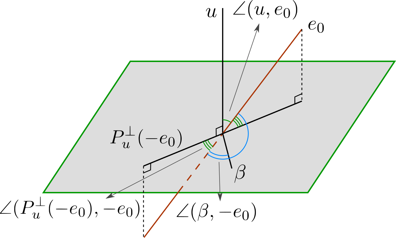
Figure 14: Demonstration of the relation between $\angle(\beta,-{\bf e}_{0})$ and ${\angle(\widetilde{{\bf e}},{\bf e}_{0})}$. In the figure, $u=\widetilde{{\bf e}}/\|\widetilde{{\bf e}}\|_{2}$.

Lemma 9.3.

$$\angle(\beta,-{\bf e}_{0})\geq\angle(P_{\widetilde{{\bf e}}}^{\perp}(-{\bf e}_{0}),-{\bf e}_{0})=\frac{\pi}{2}-\theta$$

$$\tan(\angle(\beta,-{\bf e}_{0}))\geq\tan\angle(P_{\widetilde{{\bf e}}}^{\perp}(-{\bf e}_{0}),-{\bf e}_{0})=\cot{\theta}$$

Proof.

We know that geometrically, using the property that projection of $e_{0}$ on the hyperplane with normal vector $\widetilde{{\bf e}}$ has the smallest angle among all the $\beta$ in that hyperplane, we have that if

$$\angle(\beta,-{\bf e}_{0})\geq\angle(P_{\widetilde{{\bf e}}}^{\perp}(-{\bf e}_{0}),-{\bf e}_{0})=\frac{\pi}{2}-\angle(\widetilde{{\bf e}},{\bf e}_{0})=\frac{\pi}{2}-\theta,$$

then

$$\tan\angle(\beta,-{\bf e}_{0})\geq\tan\angle(P_{\widetilde{{\bf e}}}^{\perp}(-{\bf e}_{0}),-{\bf e}_{0})=\cot{\theta}.$$

∎

Theorem 17.

The threshold $p^{\star}$ satisfies

$$p\cot\angle({\widetilde{{\bf e}},{\bf e}_{0}})\leq val(Q_{1}(\widetilde{{\bf e}}^{\prime}))\leq\cot\angle({\widetilde{{\bf e}},{\bf e}_{0}})V_{1}(\widetilde{{\bf e}}^{\prime}).$$

Proof.

First, we prove the lower bound. Let $H_{u}=\{\beta:\quad u^{T}\beta=0\}$,

$$val(Q_{1}(\widetilde{{\bf e}}^{\prime})) = \inf_{\beta\in H_{u}}[V_{1}(\beta_{(0)})\tan\angle(\beta,-{\bf e}_{0})]$$

$$\geq \inf_{\beta\in H_{u}}V_{1}(\beta_{(0)})\inf_{\beta\in H_{u}}\tan(\angle(\beta,-{\bf e}_{0}))$$

$$= p\tan{(\angle(P_{\widetilde{{\bf e}}}^{\perp}(-{\bf e}_{0}),-{\bf e}_{0}))}$$

$$= p\cot\angle({\widetilde{{\bf e}},{\bf e}_{0}})$$

Moreover, the lower bound is achieved when $\widetilde{{\bf e}}^{\prime}$ is one-sparse.

For the upper bound, we plug in $\beta=P_{\widetilde{{\bf e}}}^{\perp}(-{\bf e}_{0})$, then

$$\inf_{\|\beta\|_{2}=1,u^{T}\beta=0}\tan(\angle(\beta,-{\bf e}_{0}))V_{1}(\beta_{(0)})\leq\tan(\angle(P_{\widetilde{{\bf e}}}^{\perp}(-{\bf e}_{0}),-{\bf e}_{0}))V_{1}(P_{\widetilde{{\bf e}}}^{\perp}(-{\bf e}_{0})).$$

It is worth commenting that since $V_{1}(P_{\widetilde{{\bf e}}}^{\perp}(-{\bf e}_{0}))\leq\sqrt{p}$, and $\tan(\angle(P_{\widetilde{{\bf e}}}^{\perp}(-{\bf e}_{0}),-{\bf e}_{0}))=\cot(\angle(\widetilde{{\bf e}},{\bf e}_{0}))=\cot\theta$, we have

$$\tan(\angle(P_{\widetilde{{\bf e}}}^{\perp}(-{\bf e}_{0}),-{\bf e}_{0}))V_{1}(P_{\widetilde{{\bf e}}}^{\perp}(-{\bf e}_{0}))\leq\cot(\angle(\widetilde{{\bf e}},{\bf e}_{0}))\sqrt{p}.$$

∎

9.3 Tighter Upper and Lower Bound from Refined Analysis

Optimality by support

Assume that $\widetilde{{\bf e}}$ has $n_{e}$ non-zero entry on support $S_{\widetilde{{\bf e}}}$, we can rank the absolute value of entries of $\widetilde{{\bf e}}$ to be $|\widetilde{{\bf e}}|_{(1)},|\widetilde{{\bf e}}|_{(2)},|\widetilde{{\bf e}}|_{(3)},\ldots,|\widetilde{{\bf e}}|_{(n_{e})}$, then the entries of $\widetilde{{\bf e}}^{\prime}$ will be ranked as $|\widetilde{{\bf e}}|_{(2)},|\widetilde{{\bf e}}|_{(3)},\ldots,|\widetilde{{\bf e}}|_{(n_{e})}$.

We know the optimal solution of $(\beta^{\prime})^{\star}$ of $\inf_{\langle\widetilde{{\bf e}}^{\prime},\beta^{\prime}\rangle=1}{\mathbb{E}}_{I^{\prime}}\|\beta^{\prime}\|_{\ell_{2}(I^{\prime})}$ must have support $S_{\beta^{\star}}$ that satisfy $S_{\star}\subset S_{\widetilde{{\bf e}}^{\prime}}$. From the symmetry of objective, we know if $(\beta^{\prime})^{\star}$ is $m$ sparse, then $m\leq n_{e}-1$ and, its support must be on the top $m$ entries $|\widetilde{{\bf e}}|_{(2)},|\widetilde{{\bf e}}|_{(3)},\ldots,|\widetilde{{\bf e}}|_{(m+1)}$, we call this support $S_{m}$, and we know the corresponding entries of $(\beta^{\prime})^{\star}$ would have the same sign as entries of $\widetilde{{\bf e}}$.

We can define the $m$ sparse optimization problem for a random support function on the subset of $S_{m}$: $J_{m}\subset S_{m}$. Let $\beta$ be supported on $S_{m}$ and each entry non-negative, then

$$val(Q_{1}^{S_{m}}):=\inf_{\beta:\sum_{j=1}^{m}|\widetilde{{\bf e}}|_{(j+1)}\beta_{j}=1,\beta_{j}>0}{\mathbb{E}}_{J_{m}}\|\beta\cdot J_{m}\|_{2}$$

Let $z_{j}:=\beta_{j}|\widetilde{{\bf e}}|_{(j+1)}$, from the symmetry of objective and the order on $|\widetilde{{\bf e}}|_{(j+1)}$, we know the solution must satisfy $0<z_{m}\leq z_{m-1}\leq\ldots\leq z_{1}$. Then we can recast the optimization problem as

$$val(Q_{1}^{S_{m}}):=\inf_{z:\sum_{j=1}^{m}z_{j}=1,0<z_{m}\leq z_{m-1}\leq\ldots\leq z_{1}}{\mathbb{E}}_{B}\sqrt{\sum_{j}B_{j}\frac{1}{|\widetilde{{\bf e}}|^{2}_{(j+1)}}z_{j}^{2}}$$

As a special case, when $m=1$, $val(Q_{1}^{S_{1}})=\frac{p}{|\widetilde{{\bf e}}|_{(2)}}$ as discussed above.

Then

$$val(Q_{1}(\widetilde{{\bf e}}^{\prime}))=\inf_{m\in\{1,2,\ldots,n_{e}-1\}}val(Q_{1}^{S_{m}})$$

Tighter upper bound on $val(Q_{1})$

Now we can prove a more refine upper bound:

Lemma 9.4 (Tighter upper bound on $val(Q_{1})$).

$$val(Q_{1}(\widetilde{{\bf e}}^{\prime}))=\inf_{m\in\{1,2,\ldots,n_{e}-1\}}val(Q_{1}^{S_{m}})\leq\inf\{\frac{p}{|\widetilde{{\bf e}}|_{(2)}},\frac{V_{1}(\widetilde{{\bf e}}^{\prime}_{S_{2}})}{\|\widetilde{{\bf e}}^{\prime}_{S_{2}}\|_{2}},\frac{V_{1}(\widetilde{{\bf e}}^{\prime}_{S_{3}})}{\|\widetilde{{\bf e}}^{\prime}_{S_{3}}\|_{2}},\ldots,\frac{V_{1}(\widetilde{{\bf e}}^{\prime})}{\|\widetilde{{\bf e}}^{\prime}\|_{2}}\}$$

where

$$\cot\angle(\widetilde{{\bf e}}_{S_{m}},{\bf e}_{0})=\frac{1}{\|\widetilde{{\bf e}}^{\prime}_{S_{m}}\|_{2}}.$$

Proof of lemma 4.3.

From

$$val(Q_{1}^{S_{m}}):=\inf_{\beta:\sum_{j=1}^{m}|\widetilde{{\bf e}}|_{(j+1)}\beta_{j}=1,\beta_{j}>0}{\mathbb{E}}_{J_{m}}\|\beta\cdot J_{m}\|_{2}$$

we explore geometric point of view to find bounds.

For a fixed $m$, after re-ranking the entries by absolute value, let $S_{m}$ be the support so that only the top $m$ entries $|\widetilde{{\bf e}}|_{(2)},|\widetilde{{\bf e}}|_{(3)},\ldots,|\widetilde{{\bf e}}|_{(m+1)}$ are non-zero, let

$$|\widetilde{{\bf e}}^{\prime}|_{S_{m}}=(0,|\widetilde{{\bf e}}|_{(2)},|\widetilde{{\bf e}}|_{(3)},\ldots,|\widetilde{{\bf e}}|_{(m+1)},0,\ldots,0)$$

$$\|\widetilde{{\bf e}}^{\prime}_{S_{m}}\|_{2}^{2}=|\widetilde{{\bf e}}|^{2}_{(2)}+|\widetilde{{\bf e}}|^{2}_{(3)}+\ldots+|\widetilde{{\bf e}}|^{2}_{(m+1)}$$

let the unit vector along the direction of $|\widetilde{{\bf e}}^{\prime}|_{S_{m}}$ be

$$u^{m}=|\widetilde{{\bf e}}^{\prime}|_{S_{m}}/\|\widetilde{{\bf e}}^{\prime}_{S_{m}}\|_{2}$$

then

$$val(Q_{1}^{S_{m}}):=\frac{1}{\|\widetilde{{\bf e}}^{\prime}_{S_{m}}\|_{2}}\inf_{\beta:\beta_{j}>0}{\mathbb{E}}_{J_{m}}\|(\beta/\|\beta\|_{2})\cdot J_{m}\|_{2}\cdot\frac{1}{\sum_{j=1}^{m}u^{m}_{j}\frac{\beta_{j}}{\|\beta\|_{2}}}$$

From previous definition, since $\beta$ is supported on $S_{m}$, we denote it as $\beta^{m}$, then $V_{1}(\beta^{m})={\mathbb{E}}_{J_{m}}\|(\beta/\|\beta\|_{2})\cdot J_{m}\|_{2}$, $V_{1}(\widetilde{{\bf e}}^{\prime}_{S_{m}})=V_{1}(|\widetilde{{\bf e}}^{\prime}|_{S_{m}})=V_{1}(u^{m})$.

Geometrically,

$$\cos\angle(\beta^{m},u^{m})=\sum_{j=1}^{m}u^{m}_{j}\frac{\beta_{j}}{\|\beta\|_{2}}$$

$$\cot\angle(\widetilde{{\bf e}}_{S_{m}},{\bf e}_{0})=\frac{1}{\|\widetilde{{\bf e}}^{\prime}_{S_{m}}\|_{2}}$$

Since $\beta^{m}=u^{m}$ is a feasible point of the constraint, we have an upper bound

$$val(Q_{1}^{S_{m}})\leq\frac{V_{1}(\widetilde{{\bf e}}^{\prime}_{S_{m}})}{\|\widetilde{{\bf e}}^{\prime}_{S_{m}}\|_{2}}=\cot\angle(\widetilde{{\bf e}}_{S_{m}},{\bf e}_{0})V_{1}(\widetilde{{\bf e}}^{\prime}_{S_{m}})$$

$$val(Q_{1}^{S_{m}}) = \cot\angle(\widetilde{{\bf e}}_{S_{m}},{\bf e}_{0})\inf_{\beta:\beta_{j}>0}V_{1}(\beta^{m})\cdot\frac{1}{\cos\angle(\beta^{m},u^{m})}$$

$$= \cot\angle(\widetilde{{\bf e}}_{S_{m}},{\bf e}_{0})V_{1}(|\widetilde{{\bf e}}^{\prime}|_{S_{m}})\inf_{\beta:\beta_{j}>0}\frac{V_{1}(\beta^{m})}{V_{1}(u^{m})}\cdot\frac{1}{\cos\angle(\beta^{m},u^{m})}$$

The lower bound is given by finding the lower bound of

$$C(u^{m}):=\inf_{\beta:\beta_{j}>0}\frac{V_{1}(\beta^{m})}{V_{1}(u^{m})}\cdot\frac{1}{\cos\angle(\beta^{m},u^{m})}$$

We know upper bound $C(u^{m})\leq 1$, and lower bound $C(u^{m})\geq\frac{1}{p^{1/2}}$ based on the fact that $V_{1}\in[p,\sqrt{p}]$.

∎

10 Technical Tool: Tight Bound for Finite Difference of Objective

We study the upper and lower bound of:

$$B({\bf e}_{0},\phi):=\frac{{\mathbb{E}}_{I}\|({\bf e}_{0}+\phi)_{I}\|_{2}-{\mathbb{E}}_{I}\|({\bf e}_{0})_{I}\|_{2}}{\|\phi\|_{2}}$$

This upper and lower bound allows us to connect objective ${\mathbb{E}}_{I}\|\psi_{I}\|_{2}$ and the $2-$norm of $\psi-{\bf e}_{0}$:

$${\mathbb{E}}_{I}\|\psi_{I}\|_{2}-{\mathbb{E}}_{I}\|({\bf e}_{0})_{I}\|_{2}={\mathbb{E}}_{I}\|\psi_{I}\|_{2}-p=B({\bf e}_{0},\psi-{\bf e}_{0})\|\psi-{\bf e}_{0}\|_{2}$$

Bi-Lipschitzness of finite difference of objective near $e_{0}$ for linear constraint

We normalize the problem by defining $t:=\|\phi\|_{2},\beta:=\frac{\phi}{\|\phi\|_{2}}$. After normalization, and taking into account the linear constraint $\widetilde{{\bf e}}^{T}\phi=0$, we will study, for $\beta\in\mathcal{B}_{t}:=\{\|\beta\|_{2}=1,u^{T}\beta=0,\|e_{0}+t\beta\|_{\infty}\leq 1\}$ for finite $t$, the upper and lower bound of

$$\frac{{\mathbb{E}}_{I}\|({\bf e}_{0}+t\beta)_{I}\|_{2}-{\mathbb{E}}_{I}\|({\bf e}_{0})_{I}\|_{2}}{t}.$$

First, if $t\rightarrow 0^{+}$, then we get the directional derivative along direction of $\beta$.

$$\lim_{t\rightarrow 0^{+}}\frac{{\mathbb{E}}_{I}\|({\bf e}_{0}+t\beta)_{I}\|_{2}-{\mathbb{E}}_{I}\|({\bf e}_{0})_{I}\|_{2}}{t}.$$

Due to convexity of the function $\beta\rightarrow{\mathbb{E}}_{I}\|({\bf e}_{0}+t\beta)_{I}\|_{2}$, we have the finite difference lower bounded by directional derivative:

$$\frac{{\mathbb{E}}_{I}\|({\bf e}_{0}+t\beta)_{I}\|_{2}-{\mathbb{E}}_{I}\|({\bf e}_{0})_{I}\|_{2}}{t}\geq\lim_{t\rightarrow 0^{+}}\frac{{\mathbb{E}}_{I}\|({\bf e}_{0}+t\beta)_{I}\|_{2}-{\mathbb{E}}_{I}\|({\bf e}_{0})_{I}\|_{2}}{t}.$$

Theorem 18 (Bi-Lipschitzness of finite difference of objective near $e_{0}$ for linear constraint).

We have upper and lower bound

$$0\leq\frac{{\mathbb{E}}_{I}\|({\bf e}_{0}+t\beta)_{I}\|_{2}-{\mathbb{E}}_{I}\|({\bf e}_{0})_{I}\|_{2}}{t}-\lim_{t\rightarrow 0^{+}}\frac{{\mathbb{E}}_{I}\|({\bf e}_{0}+t\beta)_{I}\|_{2}-{\mathbb{E}}_{I}\|({\bf e}_{0})_{I}\|_{2}}{t}\leq\frac{t}{2}p\Big{(}\beta_{0}^{2}+p(1-\beta_{0}^{2})\Big{)}\leq\frac{pt}{2}.$$

This leads to

$$0\leq B({\bf e}_{0},\phi)-\nabla_{\phi}{{\mathbb{E}}_{I}\|({\bf e}_{0}+\phi)_{I}\|_{2}}\mid_{\phi=0}\leq\frac{p}{2}\|\phi\|_{2}.$$

Proof.

As mentioned before, the lower bound is derived from convexity.

In the proof, for finite $t$, we calculate the finite difference condition on $I_{0}$:

$$\frac{{\mathbb{E}}_{I}\|({\bf e}_{0}+t\beta)_{I}\|_{2}-{\mathbb{E}}_{I}\|({\bf e}_{0})_{I}\|_{2}}{t} = (1-p){\mathbb{E}}_{I}[\|\beta_{I}\|_{2}|0\not\in I]+p\big{(}\frac{{\mathbb{E}}_{I}[\|{\bf e}_{0}+t\beta_{I}\|_{2}-1|0\in I]}{t}\big{)}.$$

And

$$\lim_{t\rightarrow 0^{+}}\frac{{\mathbb{E}}_{I}\|({\bf e}_{0}+t\beta)_{I}\|_{2}-{\mathbb{E}}_{I}\|({\bf e}_{0})_{I}\|_{2}}{t} = (1-p){\mathbb{E}}_{I}[\|\beta_{I}\|_{2}|0\not\in I]+p\beta_{0}.$$

In the following, we prove an upper bound

$$\frac{{\mathbb{E}}_{I}[\|{\bf e}_{0}+t\beta_{I}\|_{2}-1|0\in I]}{t}-\beta_{0}\leq\frac{t}{2}p\|\beta_{{(0)}}\|_{2}^{2}+\frac{t}{2}\beta_{0}^{2}.$$

For finite $t$,

$$\frac{{\mathbb{E}}_{I}[\|{\bf e}_{0}+t\beta_{I}\|_{2}-1|0\in I]}{t} = {\mathbb{E}}_{I}[\left((\frac{1}{t}+\beta_{0})^{2}+\|\beta_{I_{(0)}}\|_{2}^{2}\right)^{1/2}-\frac{1}{t}|0\in I]$$

$$= \frac{1}{t}{\mathbb{E}}_{I}[\left(1+2t\beta_{0}+t^{2}\beta_{0}^{2}+t^{2}\|\beta_{I_{(0)}}\|_{2}^{2}\right)^{1/2}-1|0\in I].$$

Additionally, using concavity of the function $\sqrt{1+x}$, we have

$$\frac{1}{t}{\mathbb{E}}_{I}[\left(1+2t\beta_{0}+t^{2}\beta_{0}^{2}+t^{2}\|\beta_{I_{(0)}}\|_{2}^{2}\right)^{1/2}-1|0\in I]$$

$$\leq \frac{1}{t}[\left(1+2t\beta_{0}+t^{2}\beta_{0}^{2}+t^{2}{\mathbb{E}}_{I}\|\beta_{I_{(0)}}\|_{2}^{2}|0\in I]\right)^{1/2}-1]$$

$$= \frac{1}{t}[\left(1+2t\beta_{0}+t^{2}\beta_{0}^{2}+t^{2}p\|\beta_{{(0)}}\|_{2}^{2}\right)^{1/2}-1]$$

$$= \frac{1}{t}[\left(1+2t\beta_{0}+t^{2}\beta_{0}^{2}+t^{2}p(1-\beta_{0}^{2})\right)^{1/2}-1].$$

Now, apply the inequality: for any $x\geq-1$:

$$\sqrt{1+x}-1\leq\frac{x}{2},$$

we have

$$\frac{1}{t}[\left(1+2t\beta_{0}+t^{2}\beta_{0}^{2}+t^{2}p\|\beta_{I_{(0)}}\|_{2}^{2}\right)^{1/2}-1] \leq \beta_{0}+\frac{t}{2}(p\|\beta_{{(0)}}\|_{2}^{2}+\beta_{0}^{2}).$$

Therefore,

$$\frac{{\mathbb{E}}_{I}\|({\bf e}_{0}+t\beta)_{I}\|_{2}-{\mathbb{E}}_{I}\|({\bf e}_{0})_{I}\|_{2}}{t}-\lim_{t\rightarrow 0^{+}}\frac{{\mathbb{E}}_{I}\|({\bf e}_{0}+t\beta)_{I}\|_{2}-{\mathbb{E}}_{I}\|({\bf e}_{0})_{I}\|_{2}}{t}\leq\frac{t}{2}p\Big{(}\beta_{0}^{2}+p(1-\beta_{0}^{2})\Big{)}\leq\frac{pt}{2}.$$

The last inequality is due to $\beta_{0}^{2}\leq 1$.

∎

11 Supplementary: Main Result $2$ Proof: Guarantee for Finite Observation Window, Finite-Length Inverse

11.1 Phase Transition in Finite Observation Window, Finite-Length Inverse Setting

Finite sample setting

• Let $(X_{t})_{t\in{\mathbb{Z}}}$ be IID sampled from $pN(0,1)+(1-p)\delta_{0}$.

• The filter $a\in l_{1}({\mathbb{Z}}),(\mathcal{F}a)(\omega)\neq 0,\forall\omega\in T.$ Additionally, in finite sample setting, we assume $a^{-1}$ is zero outside of a centered window of radius $k$.

• Let $Y=a*X$ be a linear process, we are given a series of observations $(Y_{t})_{t\in[-(T+k),T+k]}$ from a centered window of radius $T+k$.

• We denote $X^{(i)}$ as the sequence being flipped and shifted for $i$ step from $X$ so that $X^{(i)}_{k}=X_{-k+i}$. Let $J_{N}$ be the support of $X$. We define the length $N=2T+1$ window as ${\cal T}:=[-T,T].$

Now we want to find an inverse filter $w=(w_{-k},\ldots,w_{0},\ldots,w_{k})\in V$ such that the convolution $w*Y$ is sparse,

$$\begin{array}[]{ll}\underset{w\in V}{\mbox{minimize}}&\frac{1}{N}\|w*Y\|_{1,{\cal T}}\\ \mbox{subject to}&(\widetilde{a}*w)_{0}=1.\end{array} {BD}_{\widetilde{a},N,k}$$ ()

Finite sample directional derivative

Now to study the finite sample convex problem, we need to calculate the directional derivative at $\psi=e_{0}$. Then

Theorem 19.

For any $X$ sequence with support $J_{N}$,

$$\lim_{t\rightarrow 0^{+}}\frac{1}{t}[(\hat{{\mathbb{E}}}\|(e_{0}+t\beta)*X\|_{1}-\hat{{\mathbb{E}}}\|e_{0}*X\|_{1})$$

$$= \langle\beta,{\frac{1}{N}\sum_{|i|\in{\cal T}}\nabla_{\psi}L_{i}}|_{e_{0}}\rangle$$

$$= \frac{1}{N}\sum_{|i|\in{\cal T}}\mbox{sign}(X_{-i})X^{(i),T}\beta$$

$$= \frac{1}{N}\left(\|X\|_{1,J_{N}}\beta_{0}+\|X*\beta_{(0)}\|_{1,{\cal T}-J_{N}}+\sum_{i\in J_{N}}(1_{X_{-i}>0}-1_{X_{-i}<0})\cdot X^{(i),T}\beta_{(0)}\right).$$

11.2 Concentration of Objective

Concentration of $\|\psi*X\|_{1}$

Lemma 11.1.

Let

$$\mu_{\mbox{min}}:=\frac{1}{\sqrt{2}\pi}\lambda_{m}(a)\sqrt{\frac{p}{k}}\|w\|_{1},$$

then it is the lower bound of ${\mathbb{E}}\frac{1}{N}\|w*a*X\|_{1,{\cal T}}$:

$${\mathbb{E}}\frac{1}{N}\|w*a*X\|_{1,{\cal T}}\geq\mu_{\mbox{min}}.$$

Now we define the intersection of $1-$norm ball of the $k-$dimensional subspace $V_{k}$ as $B_{1}(V_{k})$, then we consider $w\in B_{1}(V_{k}).$

Lemma 11.2.

Hence we consider $\psi=a*w\in a*B_{1}(V_{k}),$ and we define

$$W:=\sup_{\psi\in a*B_{1}(V_{k})}|\frac{1}{N}\sum_{j\in[-T,T]}(|(\psi*X)_{j}|-{\mathbb{E}}|(\psi*X)_{j}|)|.$$

For all $q\geq\max(2,\log(k)),$ there exists constant $C$,

$${\mathbb{E}}W^{q}\leq 2^{2q}(\frac{\lambda_{M}(a)}{N})^{q}kC^{q}(\sqrt{Npq}+q)^{q},$$

so

$$\|W\|_{q}\leq\frac{4eC}{N}\lambda_{M}(a)(\sqrt{Np(q+\log(k))}+q+\log(k)),$$

and

$$P(W>\frac{4eC\lambda_{M}(a)}{N}(\sqrt{Np\log(\frac{k}{\delta})}+\log(\frac{k}{\delta})))\leq\delta.$$

Theorem 20.

Let the solution of finite sample convex optimization be $w^{\star}$, for small $\epsilon>0$ and concentration level $\delta>0$, there exists universal constant $C$, if there are

$$N\geq k\log(\frac{k}{\delta})(\frac{C\kappa_{a}}{\epsilon})^{2},$$

and $\frac{1}{N}\leq p$, we have:

$$P(W>\epsilon\mu_{\mbox{min}})\leq\delta.$$

11.3 Concentration for Directional Derivatives

Uniform bound of directional derivatives

We define the uniform bound of directional derivatives:

$$W_{D}=\sup_{\|\beta\|_{2}=1,u^{T}\beta=0,\beta+e_{0}\in a*B_{1}(V_{k})}|\langle\beta,{\frac{1}{N}\sum_{|i|\in{\cal T}}\nabla_{\phi}L_{i}}|_{\phi=0}\rangle-\langle\beta,{\mathbb{E}}\nabla_{\phi}L|_{\phi=0}\rangle|.$$

Notice that

$$\langle\beta,{\frac{1}{N}\sum_{|i|\in{\cal T}}\nabla_{\phi}L_{i}}|_{\phi=0}\rangle-\langle\beta,{\mathbb{E}}\nabla_{\phi}L|_{\phi=0}\rangle$$

$$= \left[\frac{1}{N}\left(\|X\|_{1,J_{N}}\beta_{0}+\|X*\beta_{(0)}\|_{1,{\cal T}-J_{N}}+\sum_{i\in J_{N}}(1_{X_{-i}>0}-1_{X_{-i}<0})\cdot X^{(i),T}\beta_{(0)}\right)\right]-$$

$$\left[\sqrt{\frac{2}{\pi}}(p\cdot\beta_{0}+(1-p)\cdot{\mathbb{E}}_{I}[\|\beta_{I}\|_{2}|0\not\in I])\right].$$

Combining the following three uniform bounds on

$$|(\frac{1}{N}\|X\|_{1,J_{N}}-\sqrt{\frac{2}{\pi}}p)|,$$

$$|\frac{1}{N}\|X*\beta_{(0)}\|_{1,{\cal T}-J_{N}}-\sqrt{\frac{2}{\pi}}(1-p)\cdot{\mathbb{E}}_{I}[\|\beta_{I}\|_{2}|0\not\in I]|,$$

$$|\frac{1}{N}\sum_{i\in J_{N}}(1_{X_{-i}>0}-1_{X_{-i}<0})\cdot X^{(i),T}\beta_{(0)}|,$$

with high probability, we have

$$W_{D}<\epsilon\mu_{\mbox{min}}.$$

We define $\delta_{p}(N,\epsilon)$ the one side finite $N$ band such that for all $p<p^{\star}-\delta_{p}(N,\epsilon)$,

$$\langle\beta,{\mathbb{E}}\nabla_{\phi}L|_{\phi=0}\rangle>\epsilon\mu_{\mbox{min}}.$$

for any direction $\beta\in V,$ the directional derivative at $\phi=0$

$$\langle\beta,{\frac{1}{N}\sum_{|i|\in{\cal T}}\nabla_{\phi}L_{i}}|_{\phi=0}\rangle>0,$$

then using the convexity argument, $a*w^{\star}-e_{0}=0$.

Finite sample guarantee

From previous concentration of finite sample directional derivative, we have the following theorem.

Theorem 21.

When $a^{-1}$ is length $k$, for small constant $\epsilon>0,\delta>0$, when the number of observation $N$ satisfies

$$N\geq k\log(\frac{k}{\delta})(\frac{C\kappa_{a}}{\epsilon})^{2},$$

then

$$W_{D}<\epsilon\mu_{\mbox{min}}.$$

For $\frac{1}{N}\leq p\leq p^{\star}-\delta_{p}(N,\epsilon)$,

$$\langle\beta,{\mathbb{E}}\nabla_{\phi}L|_{\phi=0}\rangle>\epsilon\mu_{\mbox{min}}.$$

therefore, with probability $1-\delta$, for any direction $\beta\in V,$ the directional derivative at $\phi=0$

$$\langle\beta,{\frac{1}{N}\sum_{|i|\in{\cal T}}\nabla_{\phi}L_{i}}|_{\phi=0}\rangle>0,$$

the solution of finite sample convex optimization $w^{\star}$ is $a^{-1}$ up to scaling and shift with probability $1-\delta$.

11.4 Proof of Main Result $2$

Proof of theorem 19.

$$\lim_{t\rightarrow 0^{+}}\frac{1}{t}[(\hat{{\mathbb{E}}}\|(e_{0}+t\beta)*X\|_{1}-\hat{{\mathbb{E}}}\|e_{0}*X\|_{1})$$

$$= \langle\beta,{\frac{1}{N}\sum_{|i|\in{\cal T}}\nabla_{\psi}L_{i}}|_{e_{0}}\rangle$$

$$= \frac{1}{N}\sum_{|i|\in{\cal T}}\mbox{sign}(X_{0}^{(i)})X^{(i),T}\beta$$

$$= \frac{1}{N}\sum_{|i|\in{\cal T}}\mbox{sign}(X_{-i})X^{(i),T}\beta$$

$$= \frac{1}{N}\sum_{|i|\in{\cal T}}1_{X_{-i}>0}\cdot X^{(i),T}\beta+\frac{1}{N}\sum_{|i|\in{\cal T}}1_{X_{-i}<0}\cdot(-X^{(i),T}\beta)+\frac{1}{N}\sum_{|i|\in{\cal T}}1_{X_{-i}=0}\cdot|X^{(i),T}\beta|$$

$$= \frac{1}{N}\sum_{|i|\in{\cal T}}1_{X_{-i}>0}\cdot X^{(i),T}\beta+\frac{1}{N}\sum_{|i|\in{\cal T}}1_{X_{-i}<0}\cdot(-X^{(i),T}\beta)+\frac{1}{N}\sum_{|i|\in{\cal T}}|X^{(i),T}\beta_{(0)}|$$

$$= \frac{1}{N}\sum_{|i|\in{\cal T}}1_{X_{-i}>0}\cdot X_{-i}\beta_{0}+\frac{1}{N}\sum_{|i|\in{\cal T}}1_{X_{-i}<0}\cdot(-X_{-i}\beta_{0})+\frac{1}{N}\|X*\beta_{(0)}\|_{1,{\cal T}-J_{N}}+$$

$$\frac{1}{N}\sum_{|i|\in{\cal T}}1_{X_{-i}>0}\cdot X^{(i),T}\beta_{(0)}+\frac{1}{N}\sum_{|i|\in{\cal T}}1_{X_{-i}<0}\cdot(-X^{(i),T}\beta_{(0)})$$

$$= \frac{1}{N}\sum_{|i|\in{\cal T}}1_{X_{-i}\neq 0}\cdot|X_{-i}|\beta_{0}+\frac{1}{N}\|X*\beta_{(0)}\|_{1,{\cal T}-J_{N}}+\frac{1}{N}\sum_{i\in J_{N}}(1_{X_{-i}>0}-1_{X_{-i}<0})\cdot X^{(i),T}\beta_{(0)}$$

$$= \frac{1}{N}\left(\|X\|_{1,J_{N}}\beta_{0}+\|X*\beta_{(0)}\|_{1,{\cal T}-J_{N}}+\sum_{i\in J_{N}}(1_{X_{-i}>0}-1_{X_{-i}<0})\cdot X^{(i),T}\beta_{(0)}\right).$$

∎

Proof of lemma 11.1.

Without loss of generality, we rescale $w$ so that $\|w\|_{1}=1$, now

$${\mathbb{E}}_{X}Z = \frac{1}{N}\sum_{j\in[-T,T]}{\mathbb{E}}_{X}|\sum_{i=1}^{k}w_{i}(a*X)_{j-i}|$$

$$\geq \inf_{\|w\|_{1}=1}\frac{1}{N}\sum_{j\in[-T,T]}{\mathbb{E}}_{X}|\sum_{i=1}^{k}w_{i}(a*X)_{j-i}|.$$

By symmetry, we know the minimizer is $w=(\frac{1}{k},\ldots,\frac{1}{k}),$ then we use the symmetrization trick to insert a sequence of $k$ IID Rademacher ($\pm 1$) random variables $\varepsilon_{1},\ldots,\varepsilon_{k}$ in the second inequality, and then apply Khintchine inequality as the third inequality,

$${\mathbb{E}}_{X}Z \geq \frac{1}{k}\frac{1}{N}\sum_{j\in[-T,T]}{\mathbb{E}}_{X}|\sum_{i=1}^{k}(a*X)_{j-i}|$$

$$\geq \frac{1}{2}\frac{1}{k}\frac{1}{N}\sum_{j\in[-T,T]}{\mathbb{E}}_{X}|\sum_{i=1}^{k}\varepsilon_{i}(a*X)_{j-i}|$$

$$\geq \frac{1}{2}\frac{1}{k}\frac{1}{N}\sum_{j\in[-T,T]}\frac{1}{\sqrt{2}}{\mathbb{E}}_{X}\sqrt{\sum_{i=1}^{k}(a*X)^{2}_{j-i}}$$

$$\geq \frac{1}{2}\frac{1}{k}\frac{1}{N}\sum_{j\in[-T,T]}\lambda_{m}(a)\frac{1}{\sqrt{2}}{\mathbb{E}}_{X}\sqrt{\sum_{i=1}^{k}X^{2}_{j-i}}$$

$$\geq \frac{1}{2}\frac{1}{k}\frac{1}{\sqrt{2}}\frac{1}{N}\sum_{j\in[-T,T]}\lambda_{m}(a)\frac{2}{\pi}\sqrt{pk}$$

$$= \frac{1}{\sqrt{2}\pi}\lambda_{m}(a)\sqrt{\frac{p}{k}}.$$

∎

Proof of Lemma 11.2.

Let $\varepsilon_{1},\ldots,\varepsilon_{N}$ be a sequence of IID Rademacher ($\pm 1$) random variables independent of $X$. By the symmetrization inequality, see e.g. Lemma $6.3$ of book [Ledoux and Talagrand, 2013], we have the first inequality. Then since the function $t\rightarrow|t|$ is a contraction, an application of Talagrand’s contraction principle (see Lemma $8$ of [Adamczak, 2016]) with $F(x)=|x|^{q}$ conditionally on $X$ gives the second inequality.

$${\mathbb{E}}W^{q} \leq 2^{q}{\mathbb{E}}\sup_{\psi\in a*B_{1}(V_{k})}|\frac{1}{N}\sum_{j\in[-T,T]}\varepsilon_{j}|(\psi*X)_{j}||^{q}$$

$$\leq 2^{2q}{\mathbb{E}}\sup_{\psi\in a*B_{1}(V_{k})}|\frac{1}{N}\sum_{j\in[-T,T]}\varepsilon_{j}(\psi*X)_{j}|^{q}$$

$$= 2^{2q}\frac{1}{N^{q}}{\mathbb{E}}\sup_{\psi\in a*B_{1}(V_{k})}|\sum_{i\in[-T,T]}\psi_{i}\sum_{j\in[-T,T]}\varepsilon_{j}X_{j-i}|^{q}$$

$$= 2^{2q}\frac{1}{N^{q}}{\mathbb{E}}\sup_{w\in B_{1}(V_{k})}|\sum_{i\in[-T,T]}(w*a)_{i}\sum_{j\in[-T,T]}\varepsilon_{j}X_{j-i}|^{q}$$

$$\leq 2^{2q}\frac{1}{N^{q}}{\mathbb{E}}\max_{s\in[k]}|\sum_{i\in[-T,T]}a_{i-s}(\sum_{j\in[-T,T]}\varepsilon_{j}X_{j-i})|^{q}$$

$$\leq 2^{2q}(\frac{\lambda_{M}(a)}{N})^{q}\sum_{s\in[k]}{\mathbb{E}}|\sum_{j\in[-T,T]}\varepsilon_{j}X_{j-s}|^{q}.$$

Now by the moment version of Bernstein’s inequality (see Lemma $7$, equation $(18)$ of [Adamczak, 2016]), we know that there exists a universal constant $C$,

$${\mathbb{E}}|\sum_{j\in[-T,T]}\varepsilon_{j}X_{j-i}|^{q}\leq C^{q}(\sqrt{Npq}+q)^{q}.$$

Therefore,

$${\mathbb{E}}W^{q} \leq 2^{2q}(\frac{\lambda_{M}(a)}{N})^{q}\sum_{s\in[k]}{\mathbb{E}}|\sum_{j\in[-T,T]}\varepsilon_{j}X_{j-s}|^{q}$$

$$\leq 2^{2q}(\frac{\lambda_{M}(a)}{N})^{q}kC^{q}(\sqrt{Npq}+q)^{q}.$$

Then

$$\|W\|_{q}\leq\frac{4eC}{N}\lambda_{M}(a)(\sqrt{Np(q+\log(k))}+q+\log(k)).$$

Therefore, we could get the tail bound using the Chebyshev inequality for the moments,

$$P(W>\frac{4eC\lambda_{M}(a)}{N}(\sqrt{Np(q+\log(k))}+q+\log(k)))\leq e^{-q}.$$

We set $q=\log(\frac{1}{\delta})$, obtaining an upper bound for $W$ which is satisfied with probability at least $1-\delta$:

$$P(W>\frac{4eC\lambda_{M}(a)}{N}(\sqrt{Np\log(\frac{k}{\delta})}+\log(\frac{k}{\delta})))\leq\delta.$$

∎

Proof of Theorem 20.

From previous lemma, we know that with the conditions,

$$P(W>\epsilon\mu_{\mbox{min}})\leq\delta.$$

Therefore, with probability at least $1-\delta$,

$$W=\sup_{\psi\in a*B_{1}(V_{k})}|\frac{1}{N}\sum_{j\in[-T,T]}(|(\psi*X)_{j}|-{\mathbb{E}}|(\psi*X)_{j}|)|\leq\epsilon\mu_{\mbox{min}}.$$

When this is true, for all $\psi\in a*B_{1}(V_{k})$, we have a uniform bound:

$${\mathbb{E}}|(\psi*X)_{j}|-\epsilon\mu_{\mbox{min}}\leq\frac{1}{N}\sum_{j\in[-T,T]}(|(\psi*X)_{j}|\leq{\mathbb{E}}|(\psi*X)_{j}|+\epsilon\mu_{\mbox{min}}.$$

∎

Proof of Theorem 4.

Notice that

$$\langle\beta,{\frac{1}{N}\sum_{|i|\in{\cal T}}\nabla_{\phi}L_{i}}|_{\phi=0}\rangle-\langle\beta,{\mathbb{E}}\nabla_{\phi}L|_{\phi=0}\rangle$$

$$= \left[\frac{1}{N}\left(\|X\|_{1,J_{N}}\beta_{0}+\|X*\beta_{(0)}\|_{1,{\cal T}-J_{N}}+\sum_{i\in J_{N}}(1_{X_{-i}>0}-1_{X_{-i}<0})\cdot X^{(i),T}\beta_{(0)}\right)\right]-$$

$$\left[\sqrt{\frac{2}{\pi}}(p\cdot\beta_{0}+(1-p)\cdot{\mathbb{E}}_{I}[\|\beta_{I}\|_{2}|0\not\in I])\right].$$

From the previous uniform bound, with high probability, we have the following three uniform bounds on

$$|(\frac{1}{N}\|X\|_{1,J_{N}}-\sqrt{\frac{2}{\pi}}p)|,$$

$$|\frac{1}{N}\|X*\beta_{(0)}\|_{1,{\cal T}-J_{N}}-\sqrt{\frac{2}{\pi}}(1-p)\cdot{\mathbb{E}}_{I}[\|\beta_{I}\|_{2}|0\not\in I]|.$$

The uniform bound on

$$|\frac{1}{N}\sum_{i\in J_{N}}(1_{X_{-i}>0}-1_{X_{-i}<0})\cdot X^{(i),T}\beta_{(0)}|$$

comes from symmetric distribution assumption.

Combining all three uniform bounds, with high probability, we have:

$$W_{D}<\epsilon\mu_{\mbox{min}}.$$

We define $\delta_{p}(N,\epsilon)$ the one-side finite $N$ band such that for all $p<p^{\star}-\delta_{p}(N,\epsilon)$,

$$\langle\beta,{\mathbb{E}}\nabla_{\phi}L|_{\phi=0}\rangle>\epsilon\mu_{\mbox{min}}.$$

for any direction $\beta\in V,$ the directional derivative at $\phi=0$

$$\langle\beta,{\frac{1}{N}\sum_{|i|\in{\cal T}}\nabla_{\phi}L_{i}}|_{\phi=0}\rangle>0,$$

then using the convexity argument, $a*w^{\star}-e_{0}=0$.

∎

12 Supplementary: Main Result 3 Proof: Stability Guarantee with Finite Length Approximation to Infinite Length Inverse

12.0.1 Finite Length Approximation to Infinite Length Inverse Filter

Now we consider a setting where there is a kernel whose corresponding inverse kernel has infinite support, and we give a finite-length approximation.

Within the space $V_{-\infty,\infty}$ of bilaterally infinite real-valued sequences $(h(i))_{i\in{\mathbb{Z}}}$, consider the affine subspace $V_{N_{-},N_{+}}=\{(...,0,0,h_{-N_{-}},\ldots,h_{-1},1,h_{1},h_{2},\ldots,h_{N_{+}},0,0,...)\}$, an $N_{-}+N_{+}$-dimensional subspace of bilateral sequences with support at most $N_{-}+N_{+}+1$. The coordinate that is fixed to one is located at index $i=0$. Each coordinate is zero outside of a window of size $N_{-}$ on the left of zero and size $N_{+}$ on the right of zero. The special sequence $e_{0}=(\dots,0,0,1,0,0,\dots)$, vanishing everywhere except the origin, belongs to $V_{-\infty,\infty}$ and to every $V_{N_{-},N_{+}}$.

Let $a\in V_{N_{-},N_{+}}$. Then $a=(...,0,0,a_{-N_{-}},\ldots,a_{-1},1,a_{1},a_{2},\ldots,a_{N_{+}},0,0,...)$. We also write $a=e_{0}+a_{(0)}$, where $a_{(0)}\equiv(1-e_{0})\cdot a$ denotes the ‘part of $a$ supported away from location $i=0$’. We also write $a=e_{0}+a_{L}+a_{R}$, where $a_{L}=(a_{L}(i))_{i\in{\mathbb{Z}}}=(a(i)1_{\{i<0\}})_{i\in{\mathbb{Z}}}$ denotes the ‘part of $a$ supported to the left of $i=0$’ and where $a_{R}=(a_{R}(i))_{i\in{\mathbb{Z}}}=(a(i)1_{\{i>0\}})_{i\in{\mathbb{Z}}}$ denotes the ‘part of $a$ supported to the right of $i=0$’. Finally, we say that $a\in V_{N_{-},N_{+}}$ is a length $L=N_{-}+N_{+}+1$ filter.

First example: let’s look at a simple example of infinite length inverse filter approximation. Let $s\in(-1,1)$. For $a=(0,1,-s)$, then $a^{-1}=(\ldots,0,1,s,s^{2},s^{3},\ldots)$ is an infinite length inverse filter.

If we choose a length $r$ approximation $w^{r}=(\ldots,0,1,s,s^{2},s^{3},\ldots,s^{r-1})$ then

$$\|a*w^{r}-e_{0}\|_{2}^{2}=|s|^{2r}.$$

Now we consider general finite-length forward filter with infinite-length inverse filter.

12.1 Finite Length Approximation based on Z Transform

We construct the finite-length approximation filter explicitly by truncation of Z-transform.

Let the Z-transform of $a$ be

$$\begin{array}[]{ll}A(z)=\sum_{i=-s}^{t}a_{i}z^{-i}.\end{array}$$

Then Z-transform of the inverse kernel $a^{-1}$ is $1/A(z)$.

Theorem 22.

Assuming we have a finite length forward filter $a$ with its Z-transform having roots inside the unit circle, namely $s_{k}:=e^{-\rho_{k}+i\varphi_{k}}$ with $|s_{k}|<1$ and $\rho_{k}>0$ for $k\in\{-N_{-},\ldots-1,1,\ldots N_{+}\}$. Let ${\cal I}=\{-N_{-},\ldots,-1,1,\ldots,N_{+}\}$ as the set of all the possible indicies.

$$\begin{array}[]{ll}A(z)&=\sum_{i=-N_{-}}^{N_{+}}a_{i}z^{-i}\\ &=c_{0}\prod_{j=1}^{N_{-}}(1-s_{-j}z)\prod_{i=1}^{N_{+}}(1-s_{i}z^{-1}),\end{array}$$

Where $c_{0}$ is a constant to make sure that the coefficient $a_{0}=1$.

Then for a vector index $r=(r_{-N_{-}},\ldots,r_{-1},r_{1},\ldots,r_{N_{+}})$, we could construct an approximate inverse filter $w^{r}$ with Z-transform

$$\begin{array}[]{ll}W(z)&=\frac{1}{c_{0}}\prod_{j=1}^{N_{-}}(\sum_{\ell_{j}=0}^{r_{-j}-1}s^{\ell_{j}}_{-j}z^{-\ell_{j}})\prod_{i=1}^{N_{+}}(\sum_{\ell_{i}=0}^{r_{-j}-1}s^{\ell_{i}}_{i}z^{\ell_{i}})\\ &=\frac{1}{c_{0}}\prod_{j=1}^{N_{-}}(1-(s_{-j}z)^{r_{-j}})(1-s_{-j}z)^{-1}\prod_{i=1}^{N_{+}}(1-(s_{i}z^{-1})^{r_{i}})(1-s_{i}z^{-1})^{-1}.\end{array}$$

Let $\phi^{r}=w^{r}*a-e_{0}$, then

$$\begin{array}[]{ll}\|\phi^{r}\|_{2}^{2}=\|a*w^{r}-e_{0}\|_{2}^{2}&=\sum_{n=1}^{|{\cal I}|}\sum_{k_{1},\ldots,k_{n}\in{\cal I}}\exp\Big{(}-2\big{(}r_{k_{1}}\rho_{k_{1}}+\ldots+r_{k_{n}}\rho_{k_{n}}\big{)}\Big{)}.\end{array}$$

When $\min_{j}r_{j}\rightarrow\infty$, it converges to zero at an exponential rate. The convergence rate is determined by the slowest decaying exponential term as a function of $\min_{i}(r_{i}\rho_{i})$.

$$\begin{array}[]{ll}\|\phi^{r}\|_{2}&=O(\exp\Big{(}-\min_{i}(r_{i}\rho_{i})\Big{)}),\quad\min_{i}r_{i}\rightarrow\infty.\end{array}$$

12.2 Stability Theorem

Theorem 23.

Let $a\in V_{N_{-},N_{+}}$ be a forward filter with all the roots of Z-transform strictly in the unit circle. Let $w^{\star}\in V_{(r-1)N_{-},(r-1)N_{+}}$ be the solution of the convex optimization problem. Let $w^{r}$ be the constructed filter in previous theorem with a uniform vector index $(r,\ldots,r,r,\ldots,r)$. Let $\phi^{\star}=w^{\star}*a-e_{0}$, then the solution satisfy

$$\begin{array}[]{ll}B(e_{0},\phi^{\star})\|\phi^{\star}\|_{2}\leq B(e_{0},\phi^{r})\|\phi^{r}\|_{2}.\end{array}$$

Additionally, as $p<p^{\star}$, $B(e_{0},\phi^{\star})$ and $B(e_{0},\phi^{r})$ are both upper and lower bounded. Therefore, using the previous asymptotic exponential convergence bound on $\|\phi^{r}\|_{2}$ as $r\rightarrow\infty$, it converges to zero at an exponential rate

$$\begin{array}[]{ll}\|\phi^{\star}\|_{2}\leq\frac{B(e_{0},\phi^{r})}{B(e_{0},\phi^{\star})}\|\phi^{r}\|_{2}\leq O(\exp\Big{(}-r\min_{i}(\rho_{i})\Big{)}),\quad r\rightarrow\infty.\end{array}$$

12.3 Proof of Stability Theorem

Proof of Theorem 5.

Now let $\psi^{r}$ have Z-transform $\Psi(z)$, $\phi=a*w-e_{0}$ with Z-transform $\Phi(z)$,

$$\begin{array}[]{ll}\Psi(z):=A(z)W(z)&=\prod_{j=1}^{N_{-}}(1-(s_{-j}z)^{r_{-j}})\prod_{i=1}^{N_{+}}(1-(s_{i}z^{-1})^{r_{i}}).\end{array}$$

Therefore,

$$\begin{array}[]{ll}\Phi(z):=A(z)W(z)-1&=\prod_{j=1}^{N_{-}}(1-(s_{-j}z)^{r_{-j}})\prod_{i=1}^{N_{+}}(1-(s_{i}z^{-1})^{r_{i}})-1.\end{array}$$

Let ${\cal I}=\{-N_{-},\ldots,-1,1,\ldots,N_{+}\}$ as the set of all the possible indicies. And use polar representation of complex roots: for any $k\in{\cal I}=\{-N_{-},\ldots,-1,1,\ldots,N_{+}\}$

$$s_{k}:=|s_{k}|e^{i\varphi_{k}}=e^{-\rho_{k}+i\varphi_{k}},$$

where

$$\begin{array}[]{ll}\varphi_{k}:=\operatorname{Im}(\log(s_{k}))=-i\log(\frac{s_{k}}{|s_{k}|}),\end{array}$$

and since $|s_{k}|<1$ we have

$$\rho_{k}=-\operatorname{Re}(\log(s_{k}))>0.$$

Now we consider all $z=e^{2\pi it}$ on the unit circle for $t\in[\frac{-1}{2},\frac{1}{2}]$, then for any $k\in{\cal I}$

$$\begin{array}[]{ll}-(s_{k}z^{-\mbox{sign}(k)})^{r_{k}}&=-|s_{k}|^{r_{k}}\exp\big{(}i[\varphi_{k}-2\pi t\mbox{sign}(k)]\cdot r_{k}\big{)}\\ &=\exp\Big{(}-r_{k}\rho_{k}+i\cdot\big{(}r_{k}(\varphi_{k}-2\pi t\mbox{sign}(k))+\pi\big{)}\Big{)}.\end{array}$$

Now we simplify the notation by defining

$$\upsilon_{k}(t):=r_{k}(\varphi_{k}-2\pi t\mbox{sign}(k))+\pi,$$

then

$$\begin{array}[]{ll}\Phi(z)&=\prod_{j=1}^{N_{-}}(1-(s_{-j}z)^{r_{-j}})\prod_{i=1}^{N_{+}}(1-(s_{i}z^{-1})^{r_{i}})-1\\ &=\prod_{k\in{\cal I}}\Big{(}1-|s_{k}|^{r_{k}}\exp\big{(}i[\varphi_{k}-2\pi t\mbox{sign}(k)]\cdot r_{k}\big{)}\Big{)}-1\\ &=\prod_{k\in{\cal I}}\bigg{(}1+\exp\Big{(}-r_{k}\rho_{k}+i\cdot\big{(}r_{k}(\varphi_{k}-2\pi t\mbox{sign}(k))+\pi\big{)}\Big{)}\bigg{)}-1\\ &=\prod_{k\in{\cal I}}\bigg{(}1+\exp\Big{(}-r_{k}\rho_{k}+i\cdot\upsilon_{k}(t)\Big{)}\bigg{)}-1.\end{array}$$

For any $z=\exp{(2\pi it)}$ on the unit circle,

$$\begin{array}[]{ll}\Phi\big{(}\exp{(2\pi it)}\big{)}&=\prod_{k\in{\cal I}}\bigg{(}1+\exp\Big{(}-r_{k}\rho_{k}+i\cdot\upsilon_{k}(t)\Big{)}\bigg{)}-1\\ &=\sum_{n=1}^{|{\cal I}|}\sum_{k_{1},\ldots,k_{n}\in{\cal I}}\exp\Big{(}-\big{(}r_{k_{1}}\rho_{k_{1}}+\ldots+r_{k_{n}}\rho_{k_{n}}\big{)}+i\cdot\big{(}\upsilon_{k_{1}}(t)+\ldots+\upsilon_{k_{n}}(t)\big{)}\Big{)}.\end{array}$$

Additionally, for any $t\in[\frac{-1}{2},\frac{1}{2}]$,

$$\begin{array}[]{ll}|\Phi\big{(}\exp{(2\pi it)}\big{)}|^{2}=\sum_{n=1}^{|{\cal I}|}\sum_{k_{1},\ldots,k_{n}\in{\cal I}}\exp\Big{(}-2\big{(}r_{k_{1}}\rho_{k_{1}}+\ldots+r_{k_{n}}\rho_{k_{n}}\big{)}\Big{)}\end{array}$$

is independent of $t$, since the oscillation integral over the imaginary part is

$$\begin{array}[]{ll}\int_{\frac{-1}{2}}^{\frac{1}{2}}\exp\bigg{(}i\cdot\Big{(}\big{(}\upsilon_{k_{1}}(t)-\upsilon_{k_{1}}(t)\big{)}+\ldots+\big{(}\upsilon_{k_{n}}(t)-\upsilon_{k_{n}}(-t)\big{)}\Big{)}\bigg{)}dt=1.\end{array}$$

Therefore, using Fourier isometry,

$$\begin{array}[]{ll}\|\phi\|_{2}^{2}&=\int_{\frac{-1}{2}}^{\frac{1}{2}}|\Phi\big{(}\exp{(2\pi it)}\big{)}|^{2}dt\\ &=\sum_{n=1}^{|{\cal I}|}\sum_{k_{1},\ldots,k_{n}\in{\cal I}}\exp\Big{(}-2\big{(}r_{k_{1}}\rho_{k_{1}}+\ldots+r_{k_{n}}\rho_{k_{n}}\big{)}\Big{)}.\end{array}$$

When $\min_{j}r_{j}\rightarrow\infty$, it converges to zero at an exponential rate. The convergence rate is determined by the slowest decay exponential term as a function of $\min_{i}(r_{i}\rho_{i})$.

$$\begin{array}[]{ll}\|\phi^{r}\|_{2}&=O(\exp\Big{(}-\min_{i}(r_{i}\rho_{i})\Big{)}),\quad\min_{i}r_{i}\rightarrow\infty.\end{array}$$

∎

Proof of Theorem 6.

Following the previous phase transition analysis, let the directional finite difference of the objective at $e_{0}$ be $D(w)=|(w*Y)_{0}|-|X_{0}|$, $I$ be the support of $\tilde{X}$, let $\phi=w*a-e_{0}$, then we have

$$\begin{array}[]{ll}{\mathbb{E}}D(w)&=\sqrt{\frac{2}{\pi}}{\mathbb{E}}_{I}[\|(w*a)_{I}\|_{2}-\|(e_{0})_{I}\|_{2}]\\ &=\sqrt{\frac{2}{\pi}}{\mathbb{E}}_{I}[\|(e_{0}+\phi)_{I}\|_{2}-\|(e_{0})_{I}\|_{2}]\\ &=\sqrt{\frac{2}{\pi}}\|{\phi}\|_{2}B(p,\phi).\\ \end{array}$$

Now using the optimality of $w^{\star}\in V_{(r-1)N_{-},(r-1)N_{+}}$, for all $w^{r}inV_{(r-1)N_{-},(r-1)N_{+}}$, we have

$$\begin{array}[]{ll}{\mathbb{E}}_{I}[\|(w^{\star}*a)_{I}\|_{2}\leq{\mathbb{E}}_{I}[\|(w^{r}*a)_{I}\|_{2},\end{array}$$

therefore,

$$\begin{array}[]{ll}B(p,\phi^{\star})\|{\phi^{\star}}\|_{2}\leq B(p,\phi)\|{\phi}\|_{2}.\end{array}$$

Due to the bi-Lipschitz property of ${\mathbb{E}}_{I}\|(e_{0}+\phi)_{I}\|_{2}$ around $e_{0}$, we know when $p<p^{\star}$, $B(p,\phi)$ is positive and bounded by a constant.

Therefore, as $p<p^{\star}$, $B(e_{0},\phi^{\star})$ and $B(e_{0},\phi^{r})$ are both upper and lower bounded.

$$\begin{array}[]{ll}\|\phi^{\star}\|_{2}\leq\frac{B(e_{0},\phi^{r})}{B(e_{0},\phi^{\star})}\|\phi^{r}\|_{2}.\end{array}$$

Using the previous theorem,

$$\begin{array}[]{ll}\|\phi^{\star}\|_{2}\leq\frac{B(e_{0},\phi^{r})}{B(e_{0},\phi^{\star})}\sum_{n=1}^{|{\cal I}|}\sum_{k_{1},\ldots,k_{n}\in{\cal I}}\exp\Big{(}-2r\big{(}\rho_{k_{1}}+\ldots+\rho_{k_{n}}\big{)}\Big{)},\end{array}$$

using asymptotic exponential convergence bound on $\|\phi^{r}\|_{2}$ as $r\rightarrow\infty$, it converges to zero at an exponential rate

$$\begin{array}[]{ll}\|\phi^{\star}\|_{2}\leq O(\exp\Big{(}-r\min_{i}(\rho_{i})\Big{)}),\quad r\rightarrow\infty.\end{array}$$

∎

13 Supplementary: Main Result $4$ Proof: Robustness Guarantee against Stochastic and Adversarial Noises

13.1 Robustness Theorem against Stochastic Noise: Moving Average Gaussian Noise

Consider a convoluted Gaussian noise with an average standard deviation $\sigma$ and a forward moving average filter $b$ with unit norm $\|b\|_{2}=1$, then

$$\begin{array}[]{ll}Y&=a*(X+\sigma b*G).\end{array}$$

This model would include the case of IID mixture of sparse Gaussian and small Gaussian $X_{t}\sim pN(0,1)+(1-p)N(0,\sigma_{1})$ with $\sigma=\sigma_{1}$ and $b=e_{0}$. It also includes the Gaussian observation noise model

$$\begin{array}[]{ll}Y&=a*X+\sigma_{2}G_{2}=a*(X+\sigma_{2}a^{-1}*G_{2}),\end{array}$$

with $b=a^{-1}/\|a^{-1}\|_{2}$, and $\sigma=\sigma_{2}\|a^{-1}\|_{2}$.

Theorem 24.

Let $\psi^{\star}$ be the solution of the convex optimization problem in Eq.(4.1) for the moving average random noisy model

$$\begin{array}[]{ll}Y&=a*(X+\sigma b*G),\end{array}$$

then

$$B(e_{0},\psi^{\star}-e_{0})\|\psi^{\star}-e_{0}\|_{2}={\mathbb{E}}_{I}\|(\psi^{\star})_{I}\|_{2}-{\mathbb{E}}_{I}\|(e_{0})_{I}\|_{2}\leq(1-p)\sigma+p(\sqrt{1+\sigma^{2}}-1).$$

When $\sigma\leq 1,$

$$(1-p)\sigma+p(\sqrt{1+\sigma^{2}}-1)\leq\sigma,$$

therefore, when $p<p^{\star}$, $\sigma\leq 1,$ there exists a constant $C$,

$$\|\psi^{\star}-e_{0}\|_{2}\leq C\sigma.$$

13.2 Robustness Theorem against Adversarial Noise

In the adversarial noise setting, we observe

$$\begin{array}[]{ll}Y&=a*(X+\zeta)\end{array}$$

where $\zeta$ is a sequence chosen by an adversary under constraint:

$$\|\zeta\|_{\infty}\leq\eta.$$

Theorem 25.

Under adversarial noise, Let $w^{\star}$ be the solution of the population convex optimization

$$\begin{array}[]{ll}\underset{w}{\mbox{minimize}}&{\mathbb{E}}\frac{1}{N}\|w*Y\|_{\ell_{1}({\cal T}_{N})}\\ \mbox{subject to}&(\alpha*w)_{0}=1.\end{array}$$

Define $\psi^{\star}=a*w^{\star}$; then $\psi^{\star}$ satisfies the following bound:

$$\begin{array}[]{ll}B(e_{0},\psi^{\star}-e_{0})\|\psi^{\star}-e_{0}\|_{2}={\mathbb{E}}_{I}\|(\psi^{\star})_{I}\|_{2}-{\mathbb{E}}_{I}\|(e_{0})_{I}\|_{2}\leq p\sqrt{\frac{2}{\pi}}(\mathcal{R}(\eta)-1)+(1-p)\eta.\end{array}$$

Here $\mathcal{R}(\eta)$ is the folded Gaussian mean, for standard Gaussian $G$:

$$\mathcal{R}(\eta):=\sqrt{\frac{\pi}{2}}E_{G}|\eta+G|=\exp\{-\eta^{2}/2\}+\sqrt{\frac{\pi}{2}}\eta\left(1-2\Phi\left(-\eta\right)\right).$$

$\mathcal{R}(\eta)-1$ is an even function that is monotonically non-decreasing for $\eta\geq 0$ with quadratic upper and lower bound: there exists constants $C_{1}\leq C_{2}$,

$$C_{1}\eta^{2}\leq\mathcal{R}(\eta)-1\leq C_{2}\eta^{2},\forall\eta.$$

Therefore, when $p<p^{\star}$, $B(e_{0},\psi^{\star}-e_{0})$ is a bounded positive constant, there exists a constant $C$, so that

$$\|\psi^{\star}-e_{0}\|_{2}\leq C\eta,\forall\eta>0.$$

13.3 Proof of Robustness Theorem against Stochastic Noise

Proof of Theorem 7.

Consider the noisy model

$$\begin{array}[]{ll}Y&=a*(X+\sigma b*G).\end{array}$$

First,

$$\begin{array}[]{ll}F_{\sigma}(\psi)={\mathbb{E}}_{G}{\mathbb{E}}_{X}|\psi^{T}X+\sigma\psi^{T}(b*G)|={\mathbb{E}}_{G}{\mathbb{E}}_{I}|\sqrt{\|\psi_{I}\|_{2}^{2}+\sigma^{2}\|C_{b}^{T}\psi\|_{2}^{2}}G|,\end{array}$$

where $C_{b}$ is the Topelitz matrix with the first column being $b$.

Let $\psi^{\star}$ be the optimization solution, when $p<p^{\star}$, we have a chain of inequality:

$$\begin{array}[]{ll}F_{\sigma}(e_{0})\geq F_{\sigma}(\psi^{\star})\geq F_{0}(\psi^{\star})\geq F_{0}(e_{0}).\end{array}$$

We have

$$\begin{array}[]{ll}F_{\sigma}(e_{0})&={\mathbb{E}}_{G}{\mathbb{E}}_{I}|\sqrt{\|(e_{0})_{I}\|_{2}^{2}+\sigma^{2}\|b\|_{2}^{2}}G|\\ &={\mathbb{E}}_{G}{\mathbb{E}}_{I}|\sqrt{\|(e_{0})_{I}\|_{2}^{2}+\sigma^{2}}G|\\ &=\sqrt{\frac{2}{\pi}}[(1-p)\sigma+p(\sqrt{1+\sigma^{2}})].\end{array}$$

Therefore, when $p<p^{\star}$

$$\begin{array}[]{ll}F_{\sigma}(e_{0})-F_{0}(e_{0})\geq F_{0}(\psi^{\star})-F_{0}(e_{0})\geq 0.\end{array}$$

$$B(e_{0},\psi^{\star}-e_{0})\|\psi^{\star}-e_{0}\|_{2}={\mathbb{E}}_{I}\|(\psi^{\star})_{I}\|_{2}-{\mathbb{E}}_{I}\|(e_{0})_{I}\|_{2}\leq(1-p)\sigma+p(\sqrt{1+\sigma^{2}}-1).$$

When $\sigma\leq 1,$

$$(1-p)\sigma+p(\sqrt{1+\sigma^{2}}-1)\leq\sigma,$$

therefore, when $p<p^{\star}$, $\sigma\leq 1,$ there exists a constant $C$,

$$\|\psi^{\star}-e_{0}\|_{2}\leq C\sigma.$$

∎

13.4 Proof of Robustness Theorem against Adversarial Noise

Our data generative model is

$$\begin{array}[]{ll}Y&=a*(X+\zeta),\end{array}$$

where

$$\|\zeta\|_{\infty}\leq\eta.$$

Proof of Theorem 8.

The population convex optimization is

$$\begin{array}[]{ll}\underset{w,z}{\mbox{minimize}}&{\mathbb{E}}\frac{1}{N}\|w*Y\|_{\ell_{1}({\cal T}_{N})}\\ \mbox{subject to}&(\alpha*w)_{0}=1.\end{array}$$

By change of variable $\tilde{\psi}=w*a$, it could be reduced to a simpler problem

$$\begin{array}[]{ll}\mbox{minimize}_{w,s}&{\mathbb{E}}|\psi^{T}(X+\zeta)|\\ \mbox{subject to}&u^{T}\psi=1.\end{array}$$

Let $\psi^{\star}$ be the optimization solution of the worst-case objective over all possible $\zeta$, defined as $F_{\eta}(\psi)$:

$$\begin{array}[]{ll}F_{\eta}(\psi)&=\sup_{\zeta:\|\zeta\|_{\infty}\leq\eta}{\mathbb{E}}|\psi^{T}(X+\zeta)|\\ &=\sup_{\zeta:\|\zeta\|_{\infty}\leq\eta}{\mathbb{E}}_{I}|\|\psi_{I}\|_{2}G+\psi^{T}\zeta|,\end{array}$$

when $p<p^{\star}$, we have a chain of inequality:

$$\begin{array}[]{ll}F_{\eta}(e_{0})\geq F_{\eta}(\psi^{\star})\geq F_{0}(\psi^{\star})\geq F_{0}(e_{0}).\end{array}$$

Therefore, when $p<p^{\star}$

$$\begin{array}[]{ll}F_{\eta}(e_{0})-F_{0}(e_{0})\geq F(\psi(\zeta),\zeta)-F_{0}(e_{0})\geq F_{0}(\psi^{\star})-F_{0}(e_{0})\geq 0.\end{array}$$

Therefore,

$$\begin{array}[]{ll}B(e_{0},\psi^{\star}-e_{0})\|\psi^{\star}-e_{0}\|_{2}={\mathbb{E}}_{I}\|(\psi^{\star})_{I}\|_{2}-{\mathbb{E}}_{I}\|(e_{0})_{I}\|_{2}.\end{array}$$

From the folded Gaussian mean formula, let $G$ be scalar standard Gaussian, we have

$$\begin{array}[]{ll}F_{\eta}(e_{0})&=\sup_{\zeta:\|\zeta\|_{\infty}\leq\eta}{\mathbb{E}}_{I}{\mathbb{E}}_{G}|\|(e_{0})_{I}\|_{2}G+\zeta_{0}|\\ &=\sup_{\zeta:\|\zeta\|_{\infty}\leq\eta}[p{\mathbb{E}}_{G}|G+\zeta_{0}|+(1-p)|\zeta_{0}|]\\ &=\sup_{\zeta:\|\zeta\|_{\infty}\leq\eta}[p\sqrt{\frac{2}{\pi}}\mathcal{R}(\zeta_{0})+(1-p)|\zeta_{0}|]\\ &=p\sqrt{\frac{2}{\pi}}\mathcal{R}(\eta)+(1-p)\eta.\end{array}$$

The last inequality comes from the fact that $\mathcal{R}(\zeta_{0})$ is an even function that is monotonically non-decreasing for $\zeta_{0}\geq 0$. We will prove this conclusion below:

$$\begin{array}[]{ll}B(e_{0},\psi^{\star}-e_{0})\|\psi^{\star}-e_{0}\|_{2}={\mathbb{E}}_{I}\|(\psi^{\star})_{I}\|_{2}-{\mathbb{E}}_{I}\|(e_{0})_{I}\|_{2}\leq(1-p)\eta+p\sqrt{\frac{2}{\pi}}(\mathcal{R}(\eta)-1).\end{array}$$

∎

Tool: folded Gaussian mean formula

From general theory of folded Gaussian, $|\mu+\sigma G|,\quad G\sim N(0,1).$ Then its mean is

$$E_{G}|\mu+\sigma G|=\sqrt{\frac{2}{\pi}}\sigma\exp\{-\mu^{2}/(2\sigma^{2})\}+\mu\left(1-2\Phi\left(\frac{-\mu}{\sigma}\right)\right),$$ (35)

where $\Phi$ is the normal cumulative distribution function:

$$\Phi(x)=\frac{1}{\sqrt{2\pi}}\int_{-\infty}^{x}e^{-t^{2}/2}\,dt.$$

As a related remark, its variance is

$${\rm Var}_{G}|\mu+\sigma G|=E_{G}(|\mu+\sigma G|-E_{G}|\mu+\sigma G|)^{2}=\sigma^{2}+\mu^{2}-(E_{G}|\mu+\sigma G|)^{2}.$$ (36)

Lemma 13.1.

We define the ratio of folded Gaussian mean as

$$\mathcal{R}(\gamma):=\frac{E_{G}|\mu+\sigma G|}{E_{G}|\sigma G|}=\frac{E_{G}|\mu+\sigma G|}{\sqrt{\frac{2}{\pi}}\sigma}=\sqrt{\frac{\pi}{2}}E_{G}|\gamma+G|=\exp\{-\gamma^{2}/2\}+\sqrt{\frac{\pi}{2}}\gamma\left(1-2\Phi\left(-\gamma\right)\right).$$

$\mathcal{R}(\gamma)$ is an even function that is monotonically non-decreasing for $\gamma\geq 0$.

We have three different expressions (asymptotic expansion around $\gamma$) for $\mathcal{R}(\gamma)$:

$$\mathcal{R}(\gamma) = \exp\{-\gamma^{2}/2\}+\sqrt{\frac{\pi}{2}}\gamma\left(1-2\Phi\left(-\gamma\right)\right)$$ (37)

$$= \exp\{-\gamma^{2}/2\}\{1+\frac{1}{2}\gamma\left[\gamma+\frac{\gamma^{3}}{3}+\frac{\gamma^{5}}{3\cdot 5}+\cdots+\frac{\gamma^{2n+1}}{(2n+1)!!}+\cdots\right]\}$$ (38)

$$= 1+\frac{3}{2}\gamma^{2}+\frac{1}{24}\gamma^{4}-\frac{\gamma^{6}}{120}+O(\gamma^{8}).$$ (39)

When $\gamma<1,$

$$(\frac{3}{2}+\frac{1}{24})\gamma^{2}\geq\mathcal{R}(\gamma)-1\geq\frac{3}{2}\gamma^{2}.$$

When $\gamma<M$ for $M>1$, this lemma can be generalized: there exists constants $C^{\prime}\leq C$,

$$C^{\prime}\gamma^{2}\leq\mathcal{R}(\gamma)-1\leq C\gamma^{2}.$$

13.5 Technical Tool: Folded Gaussian Mean Formula

Proof for folded Gaussian mean

Proof of lemma 13.1.

Plug in the formula for mean of folded Gaussian 35, we have

$$E_{G}|\mu+\sigma G|=\sqrt{\frac{2}{\pi}}\sigma\exp\{-\gamma^{2}/2\}+\mu\left(1-2\Phi\left(-\gamma\right)\right).$$

Divide it by

$$E_{G}|\sigma G|=\sqrt{\frac{2}{\pi}}\sigma,$$

we get the first equality.

Since the CDF of the standard normal distribution can be expanded by integration by parts into a series:

$$\Phi(\gamma)=\frac{1}{2}+\frac{1}{\sqrt{2\pi}}\cdot e^{-\gamma^{2}/2}\left[\gamma+\frac{\gamma^{3}}{3}+\frac{\gamma^{5}}{3\cdot 5}+\cdots+\frac{\gamma^{2n+1}}{(2n+1)!!}+\cdots\right],$$

where $!!$ denotes the double factorial.

$$1-2\Phi(-\gamma)=\frac{1}{\sqrt{2\pi}}\cdot e^{-\gamma^{2}/2}\left[\gamma+\frac{\gamma^{3}}{3}+\frac{\gamma^{5}}{3\cdot 5}+\cdots+\frac{\gamma^{2n+1}}{(2n+1)!!}+\cdots\right].$$

This gives the second inequality.

Additionally,

$$\begin{array}[]{ll}e^{-\gamma^{2}/2}&=\sum_{n=0}^{\infty}\frac{\gamma^{2n}}{(-2)^{n}(n)!}\\ &=1-\frac{\gamma^{2}}{2}+\sum_{n=2}^{\infty}\frac{\gamma^{2n}}{(-2)^{n}(n)!},\end{array}$$

then

$$\begin{array}[]{ll}&\exp\{-\gamma^{2}/2\}\{1+\frac{1}{2}\gamma\left[\gamma+\frac{\gamma^{3}}{3}+\frac{\gamma^{5}}{3\cdot 5}+\cdots+\frac{\gamma^{2n+1}}{(2n+1)!!}+\cdots\right]\}\\ =&(\sum_{n=0}^{\infty}\frac{\gamma^{2n}}{(-2)^{n}(n)!})\{1+\frac{1}{2}\gamma\left[\sum_{n=0}^{\infty}\frac{\gamma^{2n+1}}{(2n+1)!!}\right]\}\\ =&1+\frac{3}{2}\gamma^{2}+\frac{1}{24}\gamma^{4}-\frac{\gamma^{6}}{120}+O(\gamma^{8}).\end{array}$$

Let $C_{\Phi}(\gamma^{2})$ be a function of $\gamma$, then it is a composition with the inner function being $\gamma^{2},$ defined as follows:

$$\begin{array}[]{ll}C_{\Phi}(\gamma^{2})&:=(2\Phi(\gamma)-1)/\left(\frac{\gamma}{\sqrt{2\pi}}\right)\\ &=e^{-\gamma^{2}/2}\left[1+\frac{\gamma^{2}}{3}+\frac{\gamma^{4}}{3\cdot 5}+\cdots+\frac{\gamma^{2n}}{(2n+1)!!}+\cdots\right]\\ &=[\sum_{n=0}^{\infty}\frac{\gamma^{2n}}{(2n+1)!!}]/[\sum_{n=0}^{\infty}\frac{\gamma^{2n}}{2^{n}(n)!}]\\ &=[\sum_{n=0}^{\infty}\frac{\gamma^{2n}}{(2n+1)!!}]/[\sum_{n=0}^{\infty}\frac{\gamma^{2n}}{(2n)!!}]\\ &\leq 1.\end{array}$$

We remark further that

$$\begin{array}[]{ll}C_{\Phi}(\gamma^{2})&=[\sum_{n=0}^{\infty}\frac{\gamma^{2n}}{(2n+1)!!}]/[\sum_{n=0}^{\infty}\frac{\gamma^{2n}}{(2n)!!}]\\ &=[1+\frac{\gamma^{2}}{3}++\frac{\gamma^{4}}{15}+O(\gamma^{6})]/[1+\frac{\gamma^{2}}{2}++\frac{\gamma^{4}}{8}+O(\gamma^{6})]\\ &=1-\frac{\gamma^{2}}{6}+\frac{\gamma^{4}}{40}+O(\gamma^{6}).\end{array}$$

Then

$$\begin{array}[]{ll}\mu\left(1-2\Phi\left(-\gamma\right)\right)&=\frac{1}{\sqrt{2\pi}}\cdot\mu^{2}\frac{1}{\sigma}C_{\Phi}(\gamma^{2})\\ &=\frac{1}{\sqrt{2\pi}}\cdot\mu^{2}\frac{1}{\sigma}(1-\gamma^{2}/6+O(\gamma^{4})).\\ \end{array}$$

Combining the above:

$$\begin{array}[]{ll}E_{G}|\mu+\sigma G|&=\left[\sqrt{\frac{2}{\pi}}\sigma\exp\{-\gamma^{2}/2\}+\frac{1}{\sqrt{2\pi}}\cdot\mu^{2}\frac{1}{\sigma}C_{\Phi}(\gamma^{2})\right]\\ &=\left[\sqrt{\frac{2}{\pi}}\sigma\{1-\frac{\gamma^{2}}{2}+\sum_{n=2}^{\infty}\frac{\gamma^{2n}}{(-2)^{n}(n)!}\}+\frac{1}{\sqrt{2\pi}}\cdot\mu^{2}\frac{1}{\sigma}C_{\Phi}(\gamma^{2})\right]\\ &=\sqrt{\frac{2}{\pi}}\left[\sigma\{1+(1+\frac{1}{2}\cdot C_{\Phi}(\gamma^{2}))\gamma^{2}+\sum_{n=2}^{\infty}\frac{\gamma^{2n}}{(-2)^{n}(n)!}\}\}\right].\\ \end{array}$$

Define the residual of this expansion as

$$\begin{array}[]{ll}\mbox{Res}(\gamma^{2})&:=\frac{(2\Phi(\gamma)-1)/\left(\frac{\gamma}{\sqrt{2\pi}}\right)-1}{2}\cdot\gamma^{2}+(\exp\{-\gamma^{2}/2\}-1+\gamma^{2}/2)\\ &=\frac{C_{\Phi}(\gamma^{2})-1}{2}\cdot\gamma^{2}+(\exp\{-\gamma^{2}/2\}-1+\gamma^{2}/2)\\ &=\frac{C_{\Phi}(\gamma^{2})-1}{2}\cdot\gamma^{2}+\{\sum_{n=2}^{\infty}\frac{\gamma^{2n}}{(-2)^{n}(n)!}\}\}\\ &=\frac{-\gamma^{4}}{12}+\frac{\gamma^{6}}{80}+\frac{\gamma^{4}}{(-2)^{2}(2)!}+\frac{\gamma^{6}}{(-2)^{3}(3)!}+O(\gamma^{8})\\ &=\frac{\gamma^{4}}{24}-\frac{\gamma^{6}}{120}+O(\gamma^{8}).\end{array}$$

We know that if $\gamma^{2}<1,$

$$\begin{array}[]{ll}\mbox{Res}(\gamma^{2})&=\frac{\gamma^{4}}{24}-\frac{\gamma^{6}}{120}+O(\gamma^{8})\\ &\geq 0.\end{array}$$

When $\gamma<1,$

$$(\frac{3}{2}+\frac{1}{24})\gamma^{2}\geq\mathcal{R}(\gamma)-1\geq\frac{3}{2}\gamma^{2}.$$

When $\gamma<M$ for $M>1$, this lemma can be generalized: there exist constants $C^{\prime}\leq C$,

$$C^{\prime}\gamma^{2}\leq\mathcal{R}(\gamma)-1\leq C\gamma^{2}.$$

∎

References

- [Adamczak, 2016] Adamczak, R. (2016). A note on the sample complexity of the er-spud algorithm by spielman, wang and wright for exact recovery of sparsely used dictionaries. The Journal of Machine Learning Research, 17(1):6153–6170.
- [Bai et al., 2018] Bai, Y., Jiang, Q., and Sun, J. (2018). Subgradient descent learns orthogonal dictionaries. arXiv preprint arXiv:1810.10702.
- [Bristow et al., 2013] Bristow, H., Eriksson, A., and Lucey, S. (2013). Fast convolutional sparse coding. In Proceedings of the IEEE Conference on Computer Vision and Pattern Recognition, pages 391–398.
- [Cabrelli, 1985] Cabrelli, C. A. (1985). Minimum entropy deconvolution and simplicity: A noniterative algorithm. Geophysics, 50(3):394–413.
- [Ding and Luo, 2000] Ding, Z. and Luo, Z.-Q. (2000). A fast linear programming algorithm for blind equalization. IEEE Transactions on Communications, 48(9):1432–1436.
- [Donoho, 1981] Donoho, D. (1981). On minimum entropy deconvolution. Applied Time Series Analysis 2, pages 561–608.
- [Gottlieb and Neylon, 2010] Gottlieb, L.-A. and Neylon, T. (2010). Matrix sparsification and the sparse null space problem. In Approximation, Randomization, and Combinatorial Optimization. Algorithms and Techniques, pages 205–218. Springer.
- [Heide et al., 2015] Heide, F., Heidrich, W., and Wetzstein, G. (2015). Fast and flexible convolutional sparse coding. In Proceedings of the IEEE Conference on Computer Vision and Pattern Recognition, pages 5135–5143.
- [Kennedy and Ding, 1992] Kennedy, R. A. and Ding, Z. (1992). Blind adaptive equalizers for quadrature amplitude modulated communication systems based on convex cost functions. Optical Engineering, 31(6):1189–1200.
- [Kuo et al., 2019] Kuo, H.-W., Lau, Y., Zhang, Y., and Wright, J. (2019). Geometry and symmetry in short-and-sparse deconvolution. arXiv preprint arXiv:1901.00256.
- [Kuo et al., 2020] Kuo, H.-W., Zhang, Y., Lau, Y., and Wright, J. (2020). Geometry and symmetry in short-and-sparse deconvolution. SIAM Journal on Mathematics of Data Science, 2(1):216–245.
- [Lau et al., 2019] Lau, Y., Qu, Q., Kuo, H.-W., Zhou, P., Zhang, Y., and Wright, J. (2019). Short-and-sparse deconvolution–a geometric approach. arXiv preprint arXiv:1908.10959.
- [Ledoux and Talagrand, 2013] Ledoux, M. and Talagrand, M. (2013). Probability in Banach Spaces: isoperimetry and processes. Springer Science & Business Media.
- [Spielman et al., 2012] Spielman, D. A., Wang, H., and Wright, J. (2012). Exact recovery of sparsely-used dictionaries. In Conference on Learning Theory, pages 37–1.
- [Sun et al., 2015] Sun, J., Qu, Q., and Wright, J. (2015). Complete dictionary recovery over the sphere. In 2015 International Conference on Sampling Theory and Applications (SampTA), pages 407–410. IEEE.
- [Sun et al., 2016] Sun, J., Qu, Q., and Wright, J. (2016). Complete dictionary recovery over the sphere i: Overview and the geometric picture. IEEE Transactions on Information Theory, 63(2):853–884.
- [Vembu et al., 1994] Vembu, S., Verdú, S., Kennedy, R. A., and Sethares, W. (1994). Convex cost functions in blind equalization. IEEE Transactions on Signal Processing, 42(8):1952–1960.
- [Wiggins, 1978] Wiggins, R. A. (1978). Minimum entropy deconvolution. Geoexploration, 16(1-2):21–35.
- [Zhang et al., 2018] Zhang, Y., Kuo, H.-W., and Wright, J. (2018). Structured local optima in sparse blind deconvolution. arXiv preprint arXiv:1806.00338.
- [Zhang et al., 2017] Zhang, Y., Lau, Y., Kuo, H.-w., Cheung, S., Pasupathy, A., and Wright, J. (2017). On the global geometry of sphere-constrained sparse blind deconvolution. In Proceedings of the IEEE Conference on Computer Vision and Pattern Recognition, pages 4894–4902.
- [Zibulevsky and Pearlmutter, 2000] Zibulevsky, M. and Pearlmutter, B. A. (2000). Blind source separation by sparse decomposition. In Wavelet Applications VII, volume 4056, pages 165–174. International Society for Optics and Photonics.