Optimal detection of the feature matching map in presence of noise and outliers

Abstract

We consider the problem of finding the matching map between two sets of $d$-dimensional vectors from noisy observations, where the second set contains outliers.The matching map is then an injection, which can be consistently detected only if the vectors of the second set are well separated. The main result shows that, in the high-dimensional setting, a detection region of unknown injection may be characterized by the sets of vectors for which the inlier-inlier distance is of order at least $d^{1/4}$ and the inlier-outlier distance is of order at least $d^{1/2}$. These rates are achieved using the matching minimizing the sum of logarithms of distances between matched pairs of points. We also prove lower bounds establishing optimality of these rates. Finally, we report the results of numerical experiments on both synthetic and real world data that illustrate our theoretical results and provide further insight into the properties of the algorithms studied in this work.

2106.07044

1 Introduction

Finding the best match between two clouds of points is a problem encountered in many real problems. In computer vision, one can look for correspondences between two sets of local descriptors extracted from two images. In text analysis, one can be interested in matching vector representations of the words of two similar texts, potentially in two different languages. The goal of the present work is to gain theoretical understanding of the statistical limits of the matching problem.

In the sequel, we use the notation $[n]=\{1,\ldots,n\}$ for any integer $n$, and define $\|\cdot\|$ as the Euclidean norm in $\mathbb{R}^{d}$. Assume that two independent sequences $\boldsymbol{X}=(X_{i};i\in[n])$ and $\boldsymbol{Y}=(Y_{i};i\in[n])$ of independent vectors are generated such that $X_{i}$ and $Y_{i}$ are drawn from the same distribution $P_{i}$ on $\mathbb{R}^{d}$, for every $i\in[n]$. The statistician observes the sequence $\boldsymbol{X}$ and a shuffled version $\boldsymbol{X}^{\text{\tt\#}}$ of the sequence $\boldsymbol{Y}$. More precisely, $\boldsymbol{X}^{\text{\tt\#}}$ is such that $X^{\text{\tt\#}}_{i}=Y_{\pi^{*}(i)}$ for some unobserved permutation $\pi^{*}$. The goal of matching is to infer the permutation $\pi^{*}$ from data $(\boldsymbol{X},\boldsymbol{X}^{\text{\tt\#}})$. In the case of Gaussian distributions $P_{i}$, this problem has been studied in [9, 10]. Clearly, consistent detection of the matching map $\pi^{*}$ is impossible if there are two data generating distributions $P_{i}$ and $P_{j}$ that are very close. In [9, 10], a precise quantification of the separation between these distributions is given that enables consistent detection of $\pi^{*}$. Furthermore, it is shown that the permutation minimizing the sum of logarithms of pairwise distances between the elements of $\boldsymbol{X}$ and the elements of the shuffled version $\boldsymbol{X}^{\text{\tt\#}}$ is an optimal detector of $\pi^{*}$.

In this paper, we extend the model studied in [10] to the case when the set $\boldsymbol{X}^{\text{\tt\#}}$ is contaminated by outliers. The number of outliers is supposed to be known and is equal to $m-n$, where $n=|\boldsymbol{X}|$ and $m=|\boldsymbol{X}^{\text{\tt\#}}|$ are the sizes of considered two sequences, however the indices of the outliers are unknown. All the distributions are assumed in this paper to be spherical Gaussian, although all the probabilistic tools used in the proofs have their sub-Gaussian counterparts. Thus, we consider that two spherical Gaussian distributions $P_{1}=\mathcal{N}_{d}(\mu_{1},\sigma_{1}^{2}\mathbf{I}_{d})$ and $P_{2}=\mathcal{N}_{d}(\mu_{2},\sigma_{2}^{2}\mathbf{I}_{d})$ are well separated if the “distance to noise ratio” $\kappa(P_{1},P_{2})=\|\mu_{1}-\mu_{2}\|/\sqrt{\sigma_{1}^{2}+\sigma_{2}^{2}}$ is large. Main findings of [10], in terms of smallest separation distance $\bar{\kappa}=\min_{i\neq j}\kappa(P_{i},P_{j})$ are summarized in the second columns of Table 1. Likewise, the last column of the table provides a summary of the contributions of the present paper in terms of $\bar{\kappa}_{\textup{in-in}}=\min_{i\neq j}\kappa(P_{i},P_{j})$ and $\bar{\kappa}_{\textup{in-out}}=\min_{i,j}\kappa(P_{i},Q_{j})$, where $Q_{1},\ldots,Q_{m-n}$ are the distributions of the outliers.

An unexpected finding of this work is that the “degree” of heteroscedasticity of the model has a strong impact on the separation distances and the detection regions (sets of values of $(\bar{\kappa}_{\textup{in-in}},\bar{\kappa}_{\textup{in-out}})$ for which it is possible to detect the feature map $\pi^{*}$). This is in sharp contrast with the outlier-free case, where consistent detection requires $\bar{\kappa}$ to be at least of order $(d\log n)^{1/4}$ irrespective from the behaviour of variances of $P_{i}$. We prove in this work that in the high dimensional regime $d\geq c\log n$, which is arguably more appealing than the low dimensional regime $d\leq c\log n$, the following statements are true:

• If there is no heteroscedasticity, i.e., when all the variances are equal, consistent detection of $\pi^{*}$ is possible if and only if $\bar{\kappa}=\bar{\kappa}_{\textup{in-in}}\wedge\bar{\kappa}_{\textup{in-out}}$ is at least of order $(d\log(nm))^{1/4}$. This is the same rate as in the outlier-free case.

• If the heteroscedasticity is mild, i.e., all the variances are of the same order, the condition $\bar{\kappa}_{\textup{in-in}}\gtrsim(d\log(nm))^{1/4}$ is the same as in the previous item, but the stronger condition $\bar{\kappa}_{\textup{in-out}}\gtrsim d^{1/2}$ is needed for the inlier-outlier separation distance.

• Finally, in the general heteroscedastic setting both $\bar{\kappa}_{\textup{in-in}}$ and $\bar{\kappa}_{\textup{in-out}}$ should be at least of order $d^{1/2}$. Furthermore, in all these cases consistent detection is performed by the same procedure: the Least Sum of Logarithms (LSL).

Note also that the empirical evaluation reported in the present paper shows that LSL is attractive not only from the theoretical but also from the practical point of view.

	Without outliers	With outliers
	[10]	current paper
known $\boldsymbol{\sigma}^{\text{\tt\#}}$ or all equal $\boldsymbol{\sigma}^{\text{\tt\#}}$s	LSNS is optimal $\bar{\kappa}\gtrsim(d\log n)^{1/4}$	LSNS is optimal [Thm. 1] $\bar{\kappa}_{\textup{in-in}}\wedge\bar{\kappa}_{\textup{in-out}}\gtrsim(d\log(nm))^{1/4}$
unknown $\boldsymbol{\sigma}^{\text{\tt\#}}$ $\nicefrac{{\sigma_{\max}}}{{\sigma_{\min}}}\leq C$ unknown $\boldsymbol{\sigma}^{\text{\tt\#}}$ arbitrary	LSL is optimal [5pt] $\bar{\kappa}\gtrsim(d\log n)^{1/4}$	LSL is optimal [Thm. 4] $\bar{\kappa}_{\textup{in-in}}\gtrsim(d\log(nm))^{1/4}$ & $\bar{\kappa}_{\textup{in-out}}\gtrsim d^{1/2}$ LSL is optimal [Thm. 2, 3] $\bar{\kappa}_{\textup{in-in}}\wedge\bar{\kappa}_{\textup{in-out}}\gtrsim d^{1/2}$

Table 1: A brief overview of the contributions in the high-dimensional regime $d\geq c\log n$. The table provides the condition on the normalized inlier-inlier distance $\bar{\kappa}_{\textup{in-in}}$ and inlier-outlier distance $\bar{\kappa}_{\textup{in-out}}$, making it possible to consistently detect the matching map between two sets of $d$-dimensional vectors. LSL and LSNS refer to least sum of logarithms and least sum of normalized squares, respectively.

Agenda

Section 2 describes the framework of the vector matching problem and introduces the terminology used throughout this paper. Precise statements of the main theoretical results are gathered in Section 3. The prior work is briefly discussed in Section 4. Section 5 contains numerical experiments carried out both for synthetic and real data. A brief summary and some concluding remarks are presented in Section 7. Proofs of all theoretical claims are deferred to the supplemental material.

2 Problem Formulation

We begin with formalizing the problem of matching two sequences of feature vectors $(X_{1},\ldots,X_{n})$ and $(X^{\text{\tt\#}}_{1},\ldots,X^{\text{\tt\#}}_{m})$ with different sizes $n$ and $m$ such that $m\geq n\geq 2$. In what follows, we assume that the observed feature vectors are randomly generated from the model

$$\begin{cases}X_{i}=\theta_{i}+\sigma_{i}\xi_{i}\ ,\\ X^{\text{\tt\#}}_{j}={\theta}^{\text{\tt\#}}_{j}+\sigma^{\text{\tt\#}}_{j}\xi^{\text{\tt\#}}_{j},\end{cases}\quad i=1,\ldots,n\text{ and }j=1,\ldots,m.$$ (1)

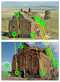
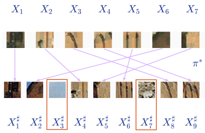
Figure 1: Illustration of the considered framework described in (1). We wish to match a set of 7 patches extracted from the first image to the 9 patches from the second image. The picture on the left shows the locations of patches as well as the true matching map $\pi^{*}$ (the yellow lines).

In this model, illustrated in Figure 1, it is assumed that

• $\boldsymbol{\theta}=(\theta_{1},\ldots,\theta_{n})$ and $\boldsymbol{\theta}^{\text{\tt\#}}=({\theta}^{\text{\tt\#}}_{1},\ldots,{\theta}^{\text{\tt\#}}_{m})$ are two sequences of vectors from $\mathbb{R}^{d}$, corresponding to the original features, which are unavailable,

• $\boldsymbol{\sigma}=(\sigma_{1},\ldots,\sigma_{n})^{\top},\boldsymbol{\sigma}^{\text{\tt\#}}=(\sigma^{\text{\tt\#}}_{1},\ldots,\sigma^{\text{\tt\#}}_{m})^{\top}$ are positive real numbers corresponding to the magnitudes of the noise contaminating each feature,

• $\xi_{1},\ldots,\xi_{n}$ and $\xi^{\text{\tt\#}}_{1},\ldots,\xi^{\text{\tt\#}}_{m}$ are two independent sequences of i.i.d. random vectors drawn from the Gaussian distribution with zero mean and identity covariance matrix.

The simplest special case of (1), considered in [10], corresponds to the situation where a perfect matching exists between the two sequences $\boldsymbol{\theta}$ and $\boldsymbol{\theta}^{\text{\tt\#}}$. This means that $m=n$ and, for some bijective mapping $\pi^{*}:[n]\to[n]$, $\theta_{i}={\theta}^{\text{\tt\#}}_{\pi(i)}$ for all $i\in[n]$. In the general case, both $\boldsymbol{X}=(X_{1},\dots,X_{n})$ and $\boldsymbol{X}^{\text{\tt\#}}=(X^{\text{\tt\#}}_{1},\dots,X^{\text{\tt\#}}_{m})$ may contain outliers, i.e. feature vectors that have no corresponding pair. In such a situation, it is merely assumed that there exists a set $S\subset[n]$ and an injective mapping $\pi^{*}:S\to[m]$ such that

$$\theta_{i}={\theta}^{\text{\tt\#}}_{\pi^{*}(i)}\quad\text{and}\quad\sigma_{i}=\sigma^{\text{\tt\#}}_{\pi^{*}(i)},\qquad\forall\,i\in S.$$ (2)

In this case we say that the vectors $\{X_{i}:i\in[n]\setminus S\}$ and $\{X^{\text{\tt\#}}_{j}:j\in[m]\setminus\pi^{*}(S)\}$ are outliers. The ultimate goal is to detect the feature matching map $\pi^{*}$.

In this work we consider the case when $S=[n]$ and $m>n$. This means that only the larger set of feature vectors, namely $\boldsymbol{X}^{\text{\tt\#}}$, contains outliers. Let us also define the set $O_{\pi^{*}}\triangleq[m]\setminus\text{Im}(\pi^{*})$, which contains the indices of outliers and satisfies $|O_{\pi^{*}}|=m-n$. Naturally, the feature vectors contained in $\boldsymbol{X}$, as well as those vectors from $\boldsymbol{X}^{\text{\tt\#}}$ that are not outliers, are called inliers.

In this formulation, the data generating distribution is defined by the parameters $\boldsymbol{\theta}^{\texttt{\#}}$, $\boldsymbol{\sigma}^{\text{\tt\#}}$ and $\pi^{*}$. We omit the set of parameters $\boldsymbol{\theta}$ and $\boldsymbol{\sigma}$, since they are automatically identified using $\pi^{*}$, $\boldsymbol{\theta}^{\texttt{\#}}$ and $\boldsymbol{\sigma}^{\text{\tt\#}}$ by the formula $(\theta_{i},\sigma_{i})=({\theta}^{\text{\tt\#}}_{\pi^{*}(i)},\sigma^{\text{\tt\#}}_{\pi^{*}(i)})$ for $i\in[n]$. Since our goal is to match the feature vectors, we focus our attention on the problem of detecting the parameter $\pi^{*}$ only, considering $\boldsymbol{\theta}^{\texttt{\#}}$ and $\boldsymbol{\sigma}^{\text{\tt\#}}$ as nuisance parameters. In what follows, we denote by $\mathbf{P}_{\boldsymbol{\theta}^{\texttt{\#}},\boldsymbol{\sigma}^{\text{\tt\#}},\pi^{*}}$ the probability distribution of the sequence $(X_{1},\ldots,X_{n},X^{\text{\tt\#}}_{1},\ldots,X^{\text{\tt\#}}_{m})$ defined by (1) under condition (2) with $S=[n]$.

We are interested in designing estimators that have an expected error smaller than a prescribed level $\alpha$ under the weakest possible conditions on the nuisance parameter $\boldsymbol{\theta}^{\texttt{\#}}$ and noise level $\boldsymbol{\sigma}^{\text{\tt\#}}$. Clearly, the problem of matching becomes more difficult with hardly distinguishable features. To quantify this phenomenon, we introduce the normalized separation distance $\bar{\kappa}_{\textup{in-in}}=\bar{\kappa}_{\textup{in-in}}(\boldsymbol{\theta}^{\texttt{\#}},\boldsymbol{\sigma}^{\text{\tt\#}},\pi^{*})$ and the normalized outlier separation distance $\bar{\kappa}_{\textup{in-out}}=\bar{\kappa}_{\textup{in-out}}(\boldsymbol{\theta}^{\texttt{\#}},\boldsymbol{\sigma}^{\text{\tt\#}},\pi^{*})$, which measure the minimal distance-to-noise ratio between inliers and the minimal distance-to-noise ratio between inliers and outliers, respectively. The precise definitions read as

$$\bar{\kappa}_{\textup{in-in}}\triangleq\min_{\begin{subarray}{c}i,j\not\in O_{\pi^{*}},\\ j\not=i\end{subarray}}\frac{\|{\theta}^{\text{\tt\#}}_{i}-{\theta}^{\text{\tt\#}}_{j}\|}{(\sigma^{\text{\tt\#}}_{i}{}^{2}+\sigma^{\text{\tt\#}}_{j}{}^{2})^{1/2}},\qquad\bar{\kappa}_{\textup{in-out}}\triangleq\min_{\begin{subarray}{c}i\not\in O_{\pi^{*}},\\ j\in O_{\pi^{*}}\end{subarray}}\frac{\|{\theta}^{\text{\tt\#}}_{i}-{\theta}^{\text{\tt\#}}_{j}\|}{(\sigma^{\text{\tt\#}}_{i}{}^{2}+\sigma^{\text{\tt\#}}_{j}{}^{2})^{1/2}}.$$ (3)

Notice that $\bar{\kappa}_{\textup{in-in}}$ can be rewritten as

$$\bar{\kappa}_{\textup{in-in}}=\min_{\begin{subarray}{c}i,j\in[n]\\ i\neq j\end{subarray}}\frac{\|\theta_{i}-\theta_{j}\|}{(\sigma_{i}^{2}+\sigma_{j}^{2})^{1/2}}.$$ (4)

Clearly, if $\bar{\kappa}_{\textup{in-in}}=0$ or, $\bar{\kappa}_{\textup{in-out}}=0$, there are two identical feature vectors in $\boldsymbol{X}^{\text{\tt\#}}$. In such a situation, assuming $\sigma_{i}$’s are all equal, the parameter $\pi^{*}$ is nonidentifiable, in the sense that there exist two different permutations $\pi^{*}_{1}$ and $\pi^{*}_{2}$ such that the distributions $\mathbf{P}_{\boldsymbol{\theta}^{\texttt{\#}},\boldsymbol{\sigma}^{\text{\tt\#}},\pi^{*}_{1}}$ and $\mathbf{P}_{\boldsymbol{\theta}^{\texttt{\#}},\boldsymbol{\sigma}^{\text{\tt\#}},\pi^{*}_{2}}$ coincide. Therefore, to ensure the existence of consistent detectors of $\pi^{*}$ it is necessary to impose the conditions $\bar{\kappa}_{\textup{in-in}}>0$ and $\bar{\kappa}_{\textup{in-out}}>0$. Moreover, good procedures are those consistently detecting $\pi^{*}$ even if either $\bar{\kappa}_{\textup{in-in}}$ or $\bar{\kappa}_{\textup{in-out}}$ are small. We are interested here in finding the detection boundary in terms of the order of magnitude of $(\bar{\kappa}_{\textup{in-in}},\bar{\kappa}_{\textup{in-out}})$. More precisely, for any given $\alpha\in(0,1)$ we wish to find a region $\mathcal{R}_{n,m,d}^{\alpha}$ in $\mathbb{R}^{2}$ such that:

• There is an estimator $\hat{\pi}_{n,m}$ of $\pi^{*}$ satisfying $\mathbf{P}_{\boldsymbol{\theta}^{\texttt{\#}},\boldsymbol{\sigma}^{\text{\tt\#}},\pi^{*}}(\hat{\pi}\neq\pi^{*})\leq\alpha$ for every $(\boldsymbol{\theta}^{\texttt{\#}},\boldsymbol{\sigma}^{\text{\tt\#}},\pi^{*})$ lying in the detection region, i.e., for which $(\bar{\kappa}_{\textup{in-in}},\bar{\kappa}_{\textup{in-out}})\in\mathcal{R}_{n,m,d}^{\alpha}$.

• There is a constant $C<1$ such that for any estimator $\bar{\pi}_{n,m}$ of $\pi^{*}$, we can find a parameter value $(\boldsymbol{\theta}^{\texttt{\#}},\boldsymbol{\sigma}^{\text{\tt\#}},\pi^{*})$ in the region $\{(\boldsymbol{\theta}^{\texttt{\#}},\boldsymbol{\sigma}^{\text{\tt\#}},\pi^{*}):(\bar{\kappa}_{\textup{in-in}},\bar{\kappa}_{\textup{in-out}})\in C\mathcal{R}_{n,m,d}^{\alpha}\}$ such that $\bar{\pi}$ fails to detect $\pi^{*}$ with a probability larger than $\alpha$.

Let us make two remarks. First, note that in the outlier-free case considered in [10], $\bar{\kappa}_{\textup{in-out}}$ is meaningless and, therefore, the detection region is one-dimensional $\mathcal{R}_{n,m,d}^{\alpha}$. Thus, it is necessarily a half-line and is proven to be of the form $\bar{\kappa}_{\textup{in-in}}\geq C(\log\nicefrac{{n}}{{\alpha}})^{1/2}\vee(d\log\nicefrac{{n}}{{\alpha}})^{1/4}$ for some universal constant $C$. Second, the aforementioned definition of the detection region $\mathcal{R}_{n,m,d}^{\alpha}$ does not guarantee its uniqueness (even up to a scaling by a universal constant). This is in contrast with the outlier-free case. To overcome this difficulty, we look for $\mathcal{R}_{n,m,d}^{\alpha}$ of the form $[t_{\textup{in-in}},+\infty)\times[t_{\textup{in-out}},+\infty)$ with the smallest possible threshold $t_{\textup{in-out}}$ for the normalized inlier-outlier distance $\bar{\kappa}_{\textup{in-out}}$.

3 Main theoretical results

In this section, we have collected the main theoretical findings of the paper. When the noise is homoscedastic, i.e., when all $\boldsymbol{\sigma}$’s are equal, the results obtained by [10] in the outlier-free setting can be easily extended to the setting with outliers. Therefore, in the present paper, we focus on the heteroscedastic case. For the sake of clarity of exposition, we will present the results in the case of known variances $\boldsymbol{\sigma},\boldsymbol{\sigma}^{\text{\tt\#}}$ prior to investigating the more interesting case of unknown variances.

The detection regions we study below are based on the maximum profile likelihood estimator. The model presented in (1) has the parameter $\boldsymbol{\Xi}=(\boldsymbol{\theta}^{\text{\tt\#}},\boldsymbol{\sigma}^{\text{\tt\#}},\pi)$, while the observations are the sequences of feature vectors $\boldsymbol{X}$ and $\boldsymbol{X}^{\text{\tt\#}}$. The negative log-likelihood of this model is given by

$$\ell_{n}(\boldsymbol{\Xi};\{\boldsymbol{X},\boldsymbol{X}^{\text{\tt\#}}\})= \sum_{i=1}^{n}\bigg{(}\frac{\|X_{i}-{\theta}^{\text{\tt\#}}_{\pi(i)}\|_{2}^{2}}{2\sigma^{\text{\tt\#}2}_{\pi(i)}}+\frac{1}{2}\log(\sigma^{\text{\tt\#}2}_{\pi(i)})\bigg{)}$$ (5)

$$+\sum_{j=1}^{m}\bigg{(}\frac{\|X^{\text{\tt\#}}_{j}-{\theta}^{\text{\tt\#}}_{j}\|_{2}^{2}}{2\sigma^{\text{\tt\#}2}_{j}}+\frac{1}{2}\log(\sigma^{\text{\tt\#}2}_{j})\bigg{)}.$$ (6)

The profile negative log-likelihood is then defined as the minimum with respect to $(\boldsymbol{\theta}^{\texttt{\#}},\boldsymbol{\sigma}^{\text{\tt\#}})$ of the log-likelihood $\ell_{n}(\boldsymbol{\Xi};\{\boldsymbol{X},\boldsymbol{X}^{\text{\tt\#}}\})$.

3.1 Warming up: known variances $\boldsymbol{\sigma},\boldsymbol{\sigma}^{\text{\tt\#}}$

One can check that the minimization with respect to $\boldsymbol{\theta}^{\texttt{\#}}$ leads to the variance-dependent cost function

$$\ell_{n}(\pi,\boldsymbol{\sigma}^{\text{\tt\#}};\{\boldsymbol{X},\boldsymbol{X}^{\text{\tt\#}}\})=\sum_{i=1}^{n}\frac{\|X_{i}-X^{\text{\tt\#}}_{\pi(i)}\|^{2}}{\sigma_{i}^{2}+\sigma^{\text{\tt\#}2}_{\pi(i)}}+\sum_{i=1}^{n}\frac{1}{2}\log(\sigma^{\text{\tt\#}2}_{\pi(i)})+\sum_{j=1}^{m}\frac{1}{2}\log(\sigma^{\text{\tt\#}2}_{j}).$$ (7)

When $m=n$ and there is no outlier, the last two sums of the last display do not depend on $\pi$ and, therefore, the maximum profile likelihood estimator of $\pi^{*}$ is obtained by the Least Sum of Normalized Squares (LSNS) criterion

$$\hat{\pi}^{\textrm{LSNS}}_{n,m}\in\operatorname*{arg\,min}_{\pi:[n]\to[m]}\sum_{i=1}^{n}\frac{\|X_{i}-X^{\text{\tt\#}}_{\pi(i)}\|^{2}}{\sigma_{i}^{2}+\sigma^{\text{\tt\#}2}_{\pi(i)}},$$ (8)

where the minimum is over all injective mappings $\pi:[n]\to[m]$. This, and the other estimators defined in this work, can be efficiently computed using suitable versions of the Hungarian algorithm [24, 25, 34]. As shows the next theorem, it turns out that even when $m>n$, the estimator $\hat{\pi}^{\textrm{LSNS}}_{n,m}$ defined above leads to an optimal detection region.

Theorem 1 (Upper bound for LSNS).

Let $\alpha\in(0,1)$ and condition (2) be fulfilled. If the separation distances $\bar{\kappa}_{\textup{in-in}}$ and $\bar{\kappa}_{\textup{in-out}}$ corresponding to $(\boldsymbol{\theta}^{\texttt{\#}},\boldsymbol{\sigma}^{\text{\tt\#}},\pi^{*})$ and defined in (3) satisfy the condition

$$\min\{\bar{\kappa}_{\textup{in-in}},\bar{\kappa}_{\textup{in-out}}\}\geq 4\Big{\{}\big{(}d\log(\nicefrac{{4nm}}{{\alpha}})\big{)}^{1/4}\vee\big{(}2\log(\nicefrac{{8nm}}{{\alpha}})\big{)}^{1/2}\Big{\}}$$ (9)

then the LSNS estimator defined in (8) detects the true matching map $\pi^{*}$ with probability at least $1-\alpha$, that is

$$\mathbf{P}_{\boldsymbol{\theta}^{\texttt{\#}},\boldsymbol{\sigma}^{\text{\tt\#}},\pi^{*}}(\hat{\pi}^{\textup{LSNS}}_{n,m}=\pi^{*})\geq 1-\alpha.$$ (10)

The similarity—both its statement and its proof— of this result to its counterpart in the outlier-free setting might suggest that the presence of outliers does not make the problem any harder from a statistical point of view. However, this is not true in the more appealing setting of unknown variances.

Remark 1.

All the results of this subsection apply in the homoscedastic case—when $\sigma_{i}=\sigma^{\text{\tt\#}}_{j}$ for all $(i,j)\in[n]\times[m]$—with unknown noise level. Indeed, in this case, the LSNS estimator coincides with the minimizer of the sum of squared errors and, therefore, does not depend on the noise levels.

Remark 2.

Theorem 1 can be readily extended to the case where the noise vectors $X_{i}-\theta_{i}$ and $X^{\text{\tt\#}}_{j}-{\theta}^{\text{\tt\#}}_{j}$ are Gaussian with zero mean and general covariance matrices, denoted respectively by $\boldsymbol{\Sigma}_{i}$ and $\boldsymbol{\Sigma}^{\text{\tt\#}}_{j}$. Then, the LSNS estimator should be defined as the minimizer of the sum over $i$ of the terms $(X_{i}-X^{\text{\tt\#}}_{\pi(i)})^{\top}(\boldsymbol{\Sigma}_{i}+\boldsymbol{\Sigma}^{\text{\tt\#}}_{\pi(i)})^{-1}(X_{i}-X^{\text{\tt\#}}_{\pi(i)})$. Hence, redefining

$$\bar{\kappa}_{\textup{in-in}}\triangleq\min_{i,j\not\in O_{\pi^{*}},j\not=i}\kappa_{ij},\qquad\bar{\kappa}_{\textup{in-out}}\triangleq\min_{i\not\in O_{\pi^{*}},j\in O_{\pi^{*}}}\kappa_{ij},$$ (11)

where $\kappa_{ij}^{2}=({\theta}^{\text{\tt\#}}_{i}-{\theta}^{\text{\tt\#}}_{j})^{\top}(\boldsymbol{\Sigma}^{\text{\tt\#}}_{i}+\boldsymbol{\Sigma}^{\text{\tt\#}}_{j})^{-1}({\theta}^{\text{\tt\#}}_{i}-{\theta}^{\text{\tt\#}}_{j})$, one gets exactly the result as the one stated in Theorem 1.

Remark 3.

The minimax setting considered in the present work is largely inspired by the corresponding setting in the problem of statistical hypotheses testing [19, 23, 48, 47, 6]. It should be noted that in many hypothesis testing problems, one can further the results on minimax rates of separation by obtaining sharp constants [14, 27, 12]. It would be interesting to investigate whether it is possible or not to obtain sharp constants in the setting of this paper. To the best of our knowledge, this question is open for other instances of multiple hypotheses testing as well.

3.2 Detection of $\pi^{*}$ for unknown and arbitrary variances $\boldsymbol{\sigma},\boldsymbol{\sigma}^{\text{\tt\#}}$

The LSNS procedure analyzed in Theorem 1 exploits the values of known noise variances to normalize the squares of distances between vectors $X_{i}$ and $X^{\text{\tt\#}}_{\pi(i)}$. Therefore, LSNS is inapplicable in the case of unknown noise variances, unless the values of all $\sigma_{i}$ and $\sigma^{\text{\tt\#}}_{i}$ are equal. Instead, we consider the Least Sum of Logarithms (LSL) estimator

$$\hat{\pi}^{\textup{LSL}}_{n,m}\triangleq\operatorname*{arg\,min}_{\pi:[n]\to[m]}\sum_{i=1}^{n}{\log\|X_{i}-X^{\text{\tt\#}}_{\pi(i)}\|^{2}},$$ (12)

where the minimum is over all injective maps $\pi:[n]\to[m]$. This estimator can be seen as the minimizer of a criterion defined as the minimum of the cost function from (7) with respect to $\boldsymbol{\sigma}^{\text{\tt\#}}$ under the constraint $\min_{j\not\in\operatorname{Im}(\pi)}\sigma^{\text{\tt\#}}_{j}\geq\sigma_{\min}$, for some fixed (but unknown) constant $\sigma_{\min}>0$.

To provide a quick overview of what follows, let us stick in the remaining of this paragraph to the case $\log(nm)=O(d)$ so that the right hand side of (9) is of order $\big{(}d\log(nm)\big{)}{}^{1/4}$. Recall that in the outlier-free case, the LSL estimator has been shown to perform as well as the LSNS while having the advantage of not requiring the knowledge of variances $\boldsymbol{\sigma}^{\text{\tt\#}}$ [10]. Somewhat unexpectedly, the situation is significantly different in the presence of outliers. Indeed, the best we managed to prove in the presence of outliers is that the detection of the matching map by LSL is possible whenever $\min\{\bar{\kappa}_{\textup{in-in}},\bar{\kappa}_{\textup{in-out}}\}\geq C\sqrt{d}$ for some sufficiently large constant $C$. The precise statement being given in the next theorem, let us mention right away that the discrepancy between this rate $\sqrt{d}$ and the rate $\big{(}d\log(nm)\big{)}{}^{1/4}$ in (9) is due to the inherent hardness of the setting and not merely an artefact of the proof. This will be made clear below.

Theorem 2 (Upper bound for LSL).

Let $\alpha\in(0,1/2)$ and condition (2) be fulfilled. If the separation distances $\bar{\kappa}_{\textup{in-in}}$ and $\bar{\kappa}_{\textup{in-out}}$ corresponding to $(\boldsymbol{\theta}^{\texttt{\#}},\boldsymbol{\sigma}^{\text{\tt\#}},\pi^{*})$ and defined by (3) satisfy

$$\min\{\bar{\kappa}_{\textup{in-in}},\bar{\kappa}_{\textup{in-out}}\}\geq\sqrt{2d}+4\Big{\{}\big{(}2d\log(\nicefrac{{4nm}}{{\alpha}})\big{)}^{1/4}\vee\big{(}3\log(\nicefrac{{8nm}}{{\alpha}}\big{)}^{1/2}\Big{\}}$$ (13)

then the LSL estimator (12) detects the matching map $\pi^{*}$ with probability at least $1-\alpha$, that is

$$\mathbf{P}_{\boldsymbol{\theta}^{\texttt{\#}},\boldsymbol{\sigma}^{\text{\tt\#}},\pi^{*}}(\hat{\pi}^{\textup{LSL}}_{n,m}=\pi^{*})\geq 1-\alpha.$$ (14)

This result is disappointing since it requires the distance between different feature vectors to be larger than $\sqrt{2d}$ in order to be able to consistently detect the matching map $\pi^{*}$. As we show below, without any further condition (for instance, on the noise variances), this rate cannot be improved. Furthermore, the rate $\sqrt{d}$ is optimal not only for LSL but also for the larger class of so called distance based $M$-estimators.

We will say that an estimator $\hat{\pi}_{n}$ of $\pi^{*}$ is a distance based $M$-estimator, if for a sequence of non-decreasing functions $\rho_{i}:\mathbb{R}_{+}\to\mathbb{R}$, $i=1,\ldots,n$, the following is correct

$$\hat{\pi}_{n}\in\operatorname*{arg\,min}_{\pi:[n]\to[m]}\sum_{i=1}^{n}\rho_{i}\big{(}\|X_{i}-X^{\text{\tt\#}}_{\pi(i)}\|\big{)},$$ (15)

where the minimum is over all injective mappings $\pi:[n]\to[m]$. We denote by $\mathcal{M}$ the set of all distance based $M$-estimators. We show that there is indeed a setup where $\bar{\kappa}_{\textup{in-in}}\wedge\bar{\kappa}_{\textup{in-out}}$ is as large as $0.2\sqrt{d}$ but any estimator from $\mathcal{M}$ fails to detect $\pi^{*}$ with probability at least $1/4$. The next theorem formalizes the described result.

Theorem 3 (Lower bound over $\mathcal{M}$).

Assume that $m>n\geq 4$ and $d\geq 422\log(4n)$. There exists a triplet $(\boldsymbol{\sigma}^{\text{\tt\#}},\boldsymbol{\theta}^{\text{\tt\#}},\pi^{*})$ such that $\bar{\kappa}_{\textup{in-in}}=\bar{\kappa}_{\textup{in-out}}=\sqrt{d/20}$ and

$$\inf_{\hat{\pi}\in\mathcal{M}}\mathbf{P}_{\boldsymbol{\theta}^{\texttt{\#}},\boldsymbol{\sigma}^{\text{\tt\#}},\pi^{*}}(\hat{\pi}\neq\pi^{*})>\nicefrac{{1}}{{4}}.$$ (16)

The proof of this theorem, postponed to the appendix, is constructive. This means that we exhibit a triplet $(\boldsymbol{\sigma}^{\text{\tt\#}},\boldsymbol{\theta}^{\text{\tt\#}},\pi^{*})$ satisfying (16). Careful inspection shows that in the case $d=O(\log(nm))$ the same triplet satisfies $\bar{\kappa}_{\textup{in-in}}\wedge\bar{\kappa}_{\textup{in-out}}\asymp\sqrt{\log(nm)}$ and (16) is still true. This implies that the order of magnitude of the right hand side of (13) is optimal both in the high-dimensional regime $d\geq 422\log(4n)$ and in the low-dimensional regime $d<422\log(4n)$. This shows the optimality of LSL among all estimators from $\mathcal{M}$. Note that the estimator $\hat{\pi}^{\textup{LSNS}}_{n,m}$ does not belong to the family of distance based M-estimators. Furthermore, in the low dimensional regime $d=O(\log(nm))$, the separation rate of the LSL, $\sqrt{\log(nm)}$, is the same as that of the LSNS.

The next theorem extends the result of Theorem 3 establishing the lower bound over all injective mappings $\pi:[n]\to[m]$, hence implying the optimality of the rate presented in Theorem 1. We show that even if $\bar{\kappa}_{\textup{in-in}}$ and $\bar{\kappa}_{\textup{in-out}}$ are of order $(d\log(nm))^{1/4}\vee(\log(nm))^{1/2}$ then there are indeed scenarios in which any estimator $\hat{\pi}$ fails to detect $\pi^{*}$ with probability at least $1/3$.

Theorem 4 (General lower bound).

Denote $\kappa=\min\{\bar{\kappa}_{\textup{in-in}},\bar{\kappa}_{\textup{in-out}}\}$. Assume that $m>n\geq 5$ and $d\geq 16\log(nm)$. Then, there exists a triplet $(\boldsymbol{\sigma}^{\text{\tt\#}},\boldsymbol{\theta}^{\text{\tt\#}},\pi^{*})$ such that $6\kappa\geq(d\log(nm))^{1/4}$ and

$$\inf_{\hat{\pi}}\mathbf{P}_{\boldsymbol{\theta}^{\text{\tt\#}},\boldsymbol{\sigma}^{\text{\tt\#}},\pi^{*}}(\hat{\pi}\neq\pi^{*})>\nicefrac{{1}}{{3}},$$ (17)

where the infimum is taken over all injective matching maps $\pi:[n]\to[m]$.

In the next section we show that under some mild conditions on $\boldsymbol{\sigma}^{\text{\tt\#}}$ it is indeed possible to obtain different rates for $\bar{\kappa}_{\textup{in-in}}$ and $\bar{\kappa}_{\textup{in-out}}$, namely we show that if $\bar{\kappa}_{\textup{in-in}}\gtrsim d^{1/4}$ and $\bar{\kappa}_{\textup{in-out}}\gtrsim d^{1/2}$ then the LSL estimator detects correct matching with high probability.

3.3 Detection of $\pi^{*}$ for unknown and mildly varying variances

The results of the last two theorems are disappointing, since they indicate that the features should be very different from one another for detection of the matching map to be possible. An interesting finding, presented below, is that strong constraint can be significantly alleviated in the context of mild heteroscedasticity. By mild heteroscedasticity we understand here the situation in which all variances $\sigma^{\text{\tt\#}}_{i}$ are of the same order of magnitude.

Theorem 5 (Upper bound under mild heteroscedasticity).

Let $r_{\sigma}=\max_{i,j}(\sigma^{\text{\tt\#}}_{i}/\sigma^{\text{\tt\#}}_{j})$. If the separation distances $\bar{\kappa}_{\textup{in-in}}$ and $\bar{\kappa}_{\textup{in-out}}$ defined in (3) satisfy

$$\bar{\kappa}_{\textup{in-in}} \geq 2\big{(}4d\log(\nicefrac{{4nm}}{{\alpha}})\big{)}^{1/4}+2\big{(}2\log(\nicefrac{{4nm}}{{\alpha}})\big{)}^{1/2}$$ (18)

$$\bar{\kappa}_{\textup{in-out}} \geq\ \sqrt{2(r_{\sigma}-1)d}+2\big{(}4r_{\sigma}^{2}d\log(\nicefrac{{4nm}}{{\alpha}})\big{)}^{1/4}+2\big{(}2r_{\sigma}\log(\nicefrac{{4nm}}{{\alpha}})\big{)}^{1/2},$$ (19)

then the LSL estimator (12) detects the matching map $\pi^{*}$ with probability at least $1-\alpha$, that is

$$\mathbf{P}_{\boldsymbol{\theta}^{\texttt{\#}},\boldsymbol{\sigma}^{\text{\tt\#}},\pi^{*}}(\hat{\pi}^{\textup{LSL}}_{n,m}=\pi^{*})\geq 1-\alpha.$$ (20)

Note that a lower bound similar to that of Theorem 3 can be proved in the case of mild heterescodestacity as well, showing that there is an example for which $\bar{\kappa}_{\textup{in-in}}$ is of order $d^{1/4}$, $\bar{\kappa}_{\textup{in-out}}$ is of order $d^{1/2}$ and any estimator from $\mathcal{M}$ fails to detect $\pi^{*}$ with probability at least $1/4$.

We complete this section by summarizing the joint contribution of Theorems 1, 2, 3 and 5. To simplify this discussion, we consider two cases: high-dimensional case refers to $d\geq\log(4nm/\alpha)$ (presented in Table 1) and low-dimensional case refers to the condition $d<\log(4nm/\alpha)$. In the high dimensional setting with arbitrary noise variances, the detection region for the LSL estimator is given by $\{\bar{\kappa}_{\textup{in-in}}\wedge\bar{\kappa}_{\textup{in-out}}\geq 15\sqrt{d}\}$, which is much worse than the detection region for LSNS, $\{\bar{\kappa}_{\textup{in-in}}\wedge\bar{\kappa}_{\textup{in-out}}\geq 8(d\log(4nm/\alpha))^{1/4}\}$, obtained in the known-variance scenario. Somewhat surprisingly, in such a setting, even a strong assumption on the outliers, such as requiring them to be at least at a distance $0.2\sqrt{d}$ of the inliers, is not enough for relaxing the assumption on the inlier-inlier separation distance. Finally, on a positive note, in the intermediate case of mildly varying variances, the detection region for the LSL estimator is of the form $\{\bar{\kappa}_{\textup{in-in}}\geq 7(d\log(4nm/\alpha))^{1/4};\ \bar{\kappa}_{\textup{in-out}}\geq 10\sqrt{d}\}$. This means that if the outliers are at a distance $\Omega(\sqrt{d})$ of the inliers, then the LSL recovers the true matching under the same condition on $\bar{\kappa}_{\textup{in-in}}$ as in the outlier-free setting.

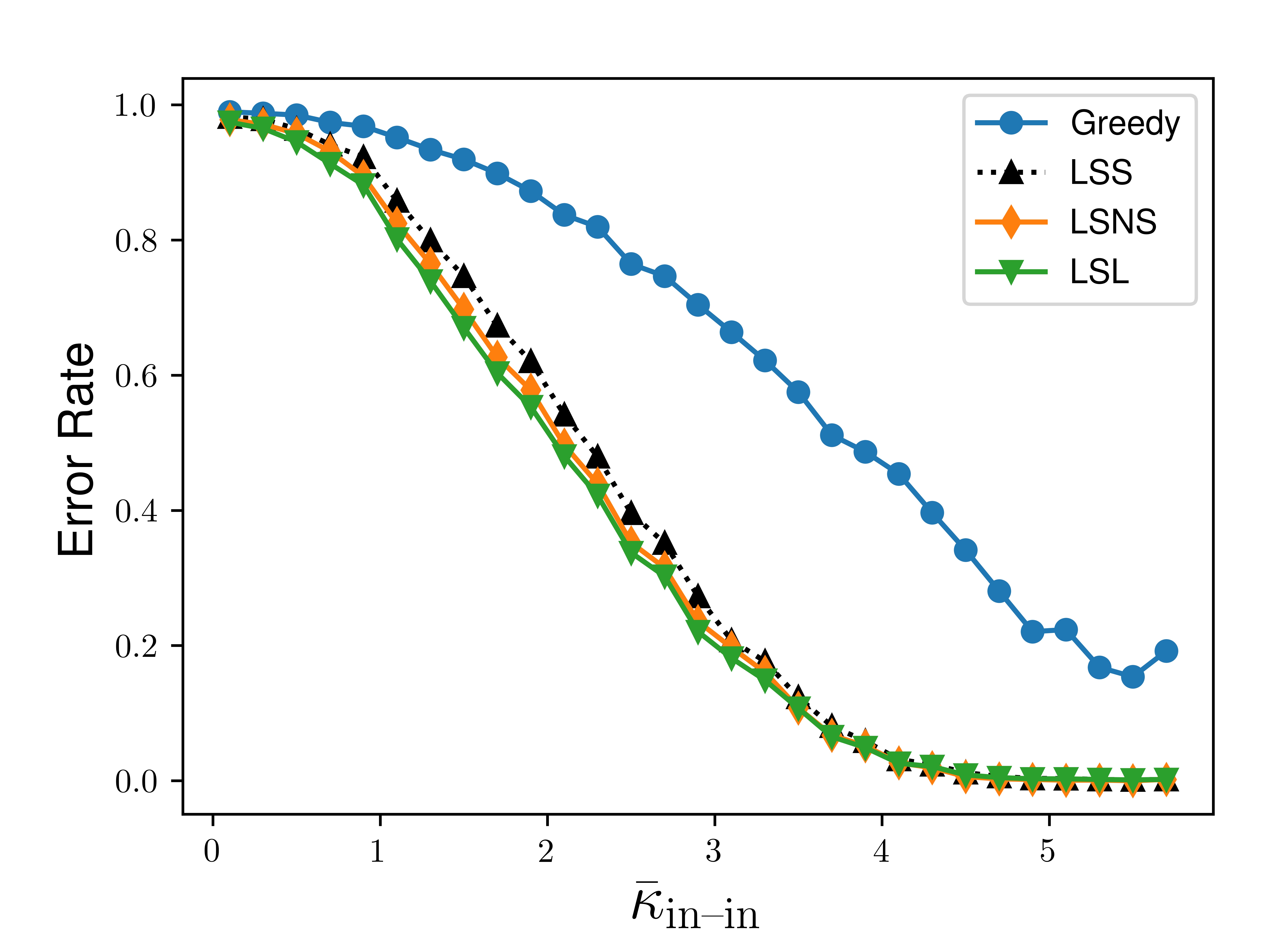
Figure 2: The performance of the methods (Greedy, LSS, LSL, LSNS) in the setup described in Exp. 1. Curves represent the error rates (percentage of repetitions in which the estimated matching map differs from the true one) as a function of separation distances. The picture illustrates that LSS, LSL and LSNS require much lower value of $\bar{\kappa}_{\textup{in-in}}$ in order to find the correct mapping.

4 Other related work

Measuring the quality of the various statistical procedures of decision making by their minimal separation rates became the standard in hypotheses testing, see the seminal papers [4, 18] and the monographs [19, 23]. Currently this approach is widely adopted in machine learning literature [51, 50, 3, 38, 49, 8]. Beyond the classical setting of two hypotheses, it can also be applied to multiple hypotheses testing framework, for instance, variable selection [35, 1, 11] or the matching problem considered here.

On the other hand, feature matching is a well studied problem in computer vision. In recent years, a great deal of attention was devoted to the acceleration of greedy matching algorithms, based on approximate and fast methods of finding nearest neighbors (e.g. [21, 45, 46, 17, 31]). Another direction that helps to improve feature matching problem is using alternative local descriptors [39, 7, 5] for given keypoints. Naturally, the question of how to chose keypoints arises, which is addressed, for instance, in [2, 42]. For more complete overview of the field we refer to [29] and references therein.

Finally, permutation estimation and related problems have been recently investigated in different contexts such as statistical seriation [15], noisy sorting [33], regression with shuffled data [37, 41], isotonic regression and matrices [32, 36, 30], crowd labeling [40], and recovery of general discrete structure [16].

5 Numerical results

In this section, we report the results of some numerical experiments carried out on simulated and real data. We applied aforementioned methods LSNS and LSL and computed different measures of their performance. To get a more complete picture, we included in this study the Least Sum of Squeres (LSS) estimator and the greedy estimator. LSS is an unnormalized version of LSNS, given by

$$\hat{\pi}^{\textrm{LSS}}_{n,m}\in\operatorname*{arg\,min}_{\pi:[n]\to[m]}\sum_{i=1}^{n}\|X_{i}-X^{\text{\tt\#}}_{\pi(i)}\|^{2}.$$ (21)

It coincides with LSNS in the case of homoscedastaic noise. The greedy estimator is obtained by sequentially matching each vector from $\boldsymbol{X}$ to the nearest vector from $\boldsymbol{X}^{\text{\tt\#}}$. Experiments were implemented using python or matlab. For solving linear sum assignment problems such as (12) or (21), the generalized and improved versions of the Hungarian algorithm were used [24, 25, 34, 13], implemented in SciPy library [44]. The goal of the first two experiments is to illustrate our theoretical findings on synthetic data sets. The third experiment aims to highlight that the methods studied in this work have some additional attractive features that would be interesting to investigate in the future.

Experiment 1: Synthetic data with random features

We first randomly generated $\pi^{*}$, $\boldsymbol{\theta}^{\texttt{\#}}$ and $\boldsymbol{\sigma}^{\text{\tt\#}}$ as follows. We randomly sampled from uniform distribution on $[0,2]$ independent variables $\tau_{ij}$, $i\in[m]$, $j\in[d]$. Then, $({\theta}^{\text{\tt\#}}_{i})_{j}$ are independently sampled from the Gaussian distribution with 0 mean and variance $\tau_{ij}$. Additionally, for every ${\theta}^{\text{\tt\#}}_{i}\in\boldsymbol{\theta}^{\texttt{\#}}$ such that $i\notin J_{\pi^{*}}$ (${\theta}^{\text{\tt\#}}_{i}$ is an outlier), we incremented every coordinate of ${\theta}^{\text{\tt\#}}_{i}$ by $i$. Entries of $\boldsymbol{\sigma}^{\text{\tt\#}}$ were sampled from the uniform distribution over $[0.5,2]$. Sequences $\boldsymbol{X}$ and $\boldsymbol{X}^{\text{\tt\#}}$ were generated according to Section 2 with $\pi^{*}(i)=i$ for $i\in[n]$. We applied to this data the following matching algorithms: Greedy, LSS, LSNS and LSL.

We chose $n=100$, $m=130$ and $d=50$, and generated $N=50$ datasets according to the foregoing process. For each dataset, we computed the 0-1 error of the considered estimators and the values of $(\bar{\kappa}_{\textup{in-in}},\bar{\kappa}_{\textup{in-out}})$. We plotted in Figure 2 the error averaged over all datasets with a given value of $\bar{\kappa}_{\textup{in-in}}$. We see that the error decreases fast with $\bar{\kappa}_{\textup{in-in}}$, corroborating our theoretical results.

Experiment 2: Synthetic data with deterministic features

The second experiment is conducted on data generated by features $\boldsymbol{\theta}^{\texttt{\#}}$ and variances $\boldsymbol{\sigma}^{\text{\tt\#}}$ inspired by the example constructed in the proof of Theorem 3. More precisely, for some real numbers $a$ and $b$ representing, respectively, the scale of inlier-inlier distance $\bar{\kappa}_{\textup{in-in}}$ and inlier-outlier distance $\bar{\kappa}_{\textup{in-out}}$, we set ${\theta}^{\text{\tt\#}}_{k}=[ka,0,\ldots,0]^{\top}$ for $k\in[n]$ and ${\theta}^{\text{\tt\#}}_{n+k}=[na+kb,0,\ldots,0]^{\top}$. We also used decreasing variances $\sigma^{\text{\tt\#}}_{k}=1/k^{3/2}$ for $k\in[m]$ and true identity mapping $\pi^{*}(k)=k$ for $k\in[n]$. We chose $n=100$, $m=120$ and dimension $d$ varying in the set $\{10,20,40\}$. For each pair of values $(a,b)$ in a suitably chosen grid, we repeated $n_{\textup{rep}}=400$ times the experiment that consisted in generating data according to (1) and computing estimators $\hat{\pi}_{n,m}^{\textup{LSS}}$ and $\hat{\pi}_{n,m}^{\textup{LSL}}$ defined respectively by (21) and (12). We then computed, for each pair $(a,b)$ and for each estimator LSS and LSL, the percentage of successful detection among $n_{\textup{rep}}$ repetitions.

The obtained detection regions are depicted in Figure 3 in the form of heatmaps. This visualisation allows us to grasp the forms of the detection regions for the specific choice of parameters considered in this example. The first observation is that LSL is clearly superior to LSS for all the considered values of the dimension. Second, we clearly see the deterioration of the detection region when the dimension $d$ becomes larger. Third, the values of $\bar{\kappa}_{\textup{in-out}}$ used in the plots are at least one order of magnitude larger than those of $\bar{\kappa}_{\textup{in-in}}$. This is in line with the claim of Theorem 5. We also observe in these pictures that successful detection occurs when $\bar{\kappa}_{\textup{in-out}}$ is larger than some threshold even if $\bar{\kappa}_{\textup{in-in}}$ is small. This must be a nice feature of LSL and LSS in this specific example, which unfortunately does not generalize to other examples as shown by our theoretical results.

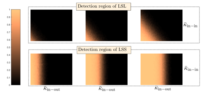
Figure 3: Heatmaps of the error rate of the LSL (top row) and the LSS (bottom row) estimators in Experiment 2. We chose $n=100$, $m=120$ and $d\in\{10,20,40\}$ from left to right. The parameter $a$ representing the scale of $\bar{\kappa}_{\textup{in-in}}$ and corresponding to $y$-axis varies from 0.02 to 0.08, whereas $b$ representing the scale of $\bar{\kappa}_{\textup{in-out}}$ and corresponding to $x$-axis varies from 0.3 to 10. Dark colour means that probability of successful detection is close to 1 (error rate close to zero).

Experiment 3: Real data example

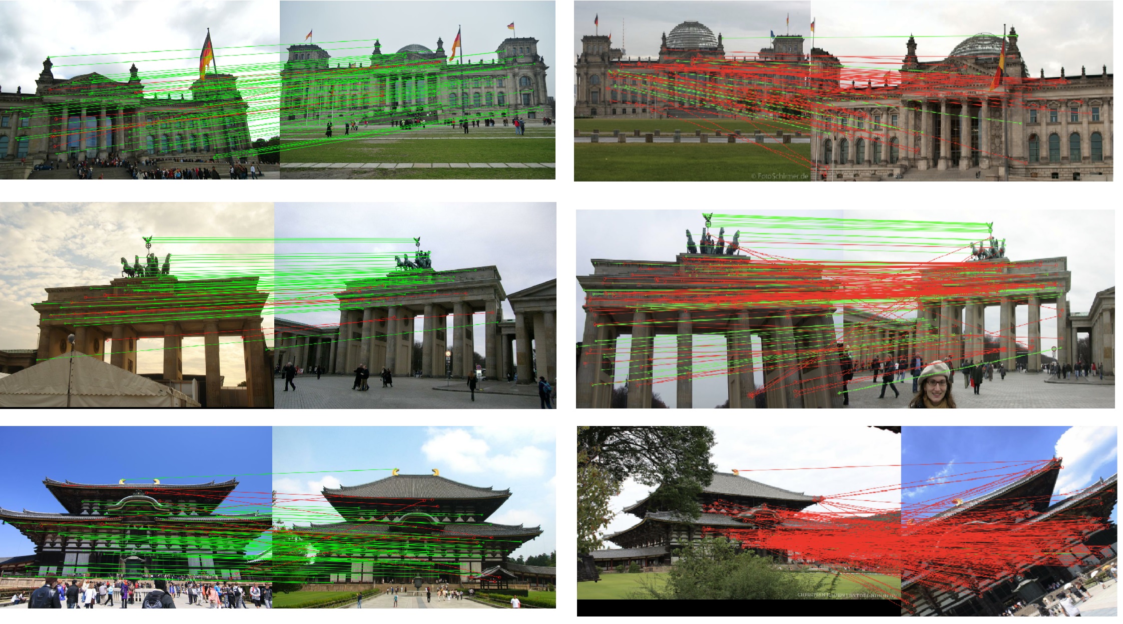
Figure 6: Matching map computed by LSL on randomly chosen easy (not challenging) and challenging pairs of images from each scene. The green lines represent the correct matching, and red lines are incorrect ones.

This experiment is conducted on the IMC-PT 2020 dataset from [22] that consists of images of 16 different scenes with corresponding 3D point-clouds of landmarks, which are used to obtain (pseudo) ground-truth local keypoint matchings. For a given scene, we sampled 1000 pairs of distinct images of the same landmark with different camera locations, angles, weather conditions etc. For each image pair we generated 2D keypoints from original set of 3D points (note that the same 3D point appears in both of the images, so we have ground truth keypoint matching between 2 images). Subsequently, we computed SIFT descriptors [28] for every keypoint in images using Python OpenCV interface [20]. Some pairs of images being more challenging than others, we split the dataset into two sets of image pairs in order to gain more understanding on the behaviour of the algorithms. The challenging pairs are those for which the OpenCV default matching algorithm has accuracy less than $50\%$. To give a glimpse of what easy and challenging pairs of images look like we show in Figure 6 image pairs with accuracy of OpenCV matching algorithm larger than $50\%$ and image pairs with accuracy smaller than $50\%$ from each scene.

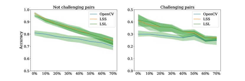
Figure 4: The estimation accuracy measured in the Hamming loss of the estimated matching in Exp. 3 for different values of the outlier rate, $(m-n)/n$, varying from $0\%$ to $70\%$. The medians of estimation accuracy both for challenging pairs (right plot) and simple pairs (left plot) of images from Temple Nara scene was computed using OpenCV, LSS and LSL matchers. The green region represents the interquartile range (lower and upper bounds being $25\%$ and $75\%$ percentiles, respectively).

Then, for every image pair, we fixed randomly chosen 100 keypoints in the first image (and corresponding keypoints in the second image) and added outliers to the second image from the remaining keypoints. The outlier rate is chosen to be between $0\%$ to $70\%$. Finally, 3 descriptor matching algorithms were applied (OpenCV default matching algorithm, LSS and LSL). Note that $\boldsymbol{\sigma}$ and $\boldsymbol{\sigma}^{\text{\tt\#}}$ from (1) are unknown, hence LSNS is not applicable. One can consider using the estimates $\hat{\boldsymbol{\sigma}}$ and $\boldsymbol{\hat{\sigma}}^{\text{\tt\#}}$ instead of $\boldsymbol{\sigma}$ and $\boldsymbol{\sigma}^{\text{\tt\#}}$ in (8), but this is beyond the scope of this paper.

The median estimation accuracy measured in the Hamming loss—for the image pairs from Temple Nara Japan scene—is plotted in Figure 4. The error bars with borderlines corresponding to $75\%$ and $25\%$ percentiles are also displayed. The first observation is that LSS and LSL outperform the OpenCV matcher in terms of the number of erroneous matches. Second, the rate of correctly matched descriptors deteriorates with the growth of outlier rate and this deterioration seems to be linear. This contrasts with our theoretical results in which which the impact of the rate of outliers is very limited. Note, however, that in the present experiment the outliers can be very similar to the inliers and, therefore, the separation condition imposed on $\bar{\kappa}_{\textup{in-out}}$ in Theorems 2 and 5 is violated. In addition, the results established in this work deal with the error of detection of matching map and do not assess the proportion of correctly matched descriptors.

We also plot the boxplots of the distances between SIFT descriptors of matching and non-matching keypoints both for easy (not challenging) and challenging pairs of images. Figure 5 has 3 plots for each of the scenes and 4 boxplots in each of them. The first 2 boxplots correspond to the distance between SIFT descriptors of matching and non-mathcing keypoints for easy pairs, while the last 2 boxplots are that of challenging pairs. There are several phenomena that are observed across all scenes. First, the median distance for matching keypoint descriptors is much smaller than that of non-matching keypoint descriptors. Second, the median distance between the matching keypoint descriptors from challenging pairs is much higher than that of easy pairs. We also observe that the distance distribution of non-matching keypoint descriptors is roughly the same for easy and challenging pairs.

The results of this experiment suggest that LSL and LSS are good estimators in this more general setting as well (descriptors which are not well separated). However, the number of outliers might have a significant impact on the accuracy of the distance-based algorithms and this impact needs to be better understood.

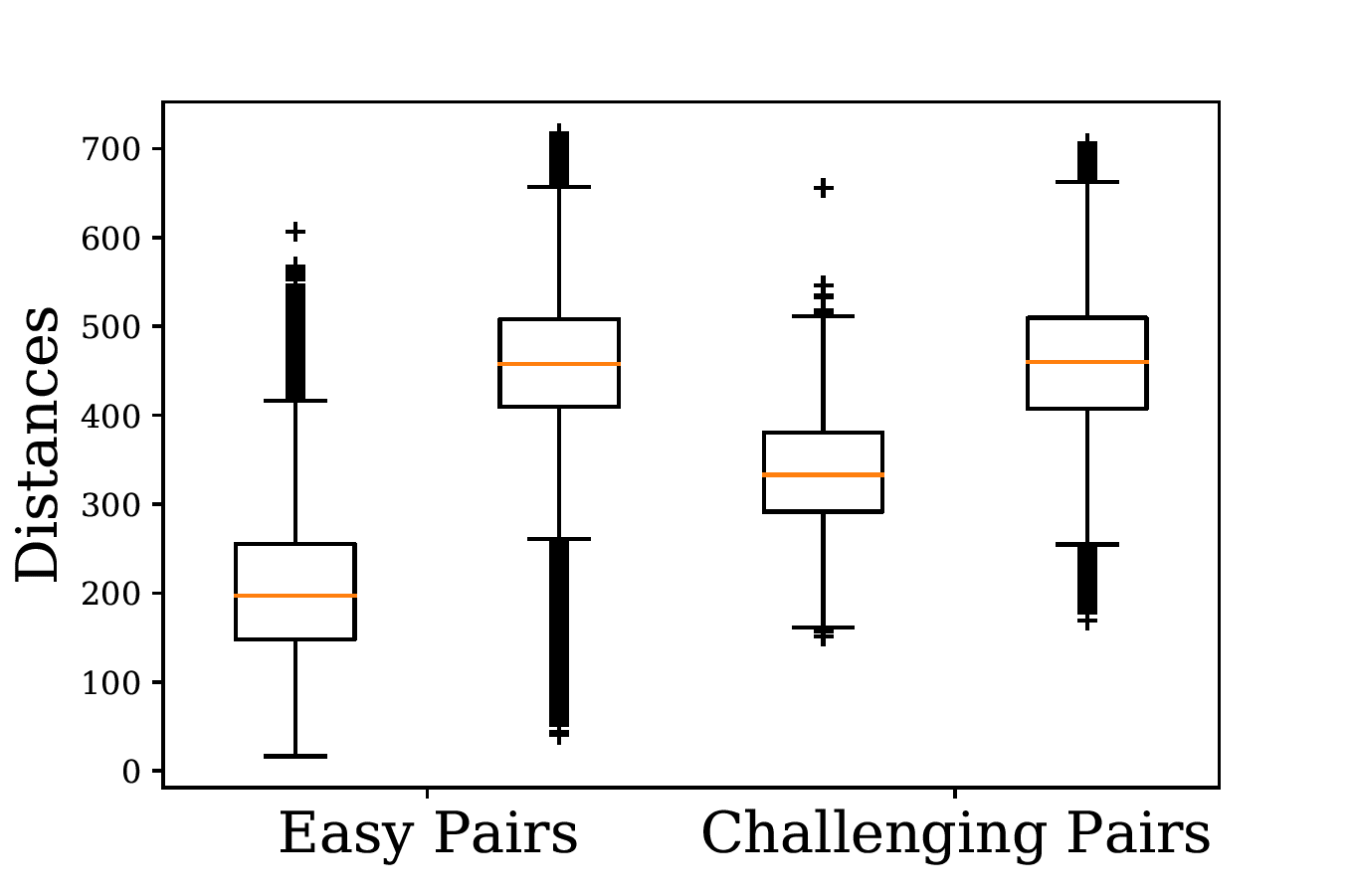
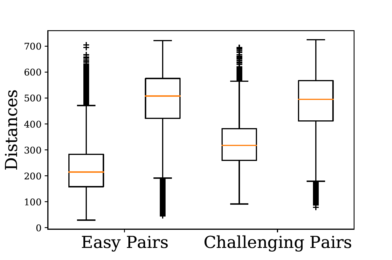
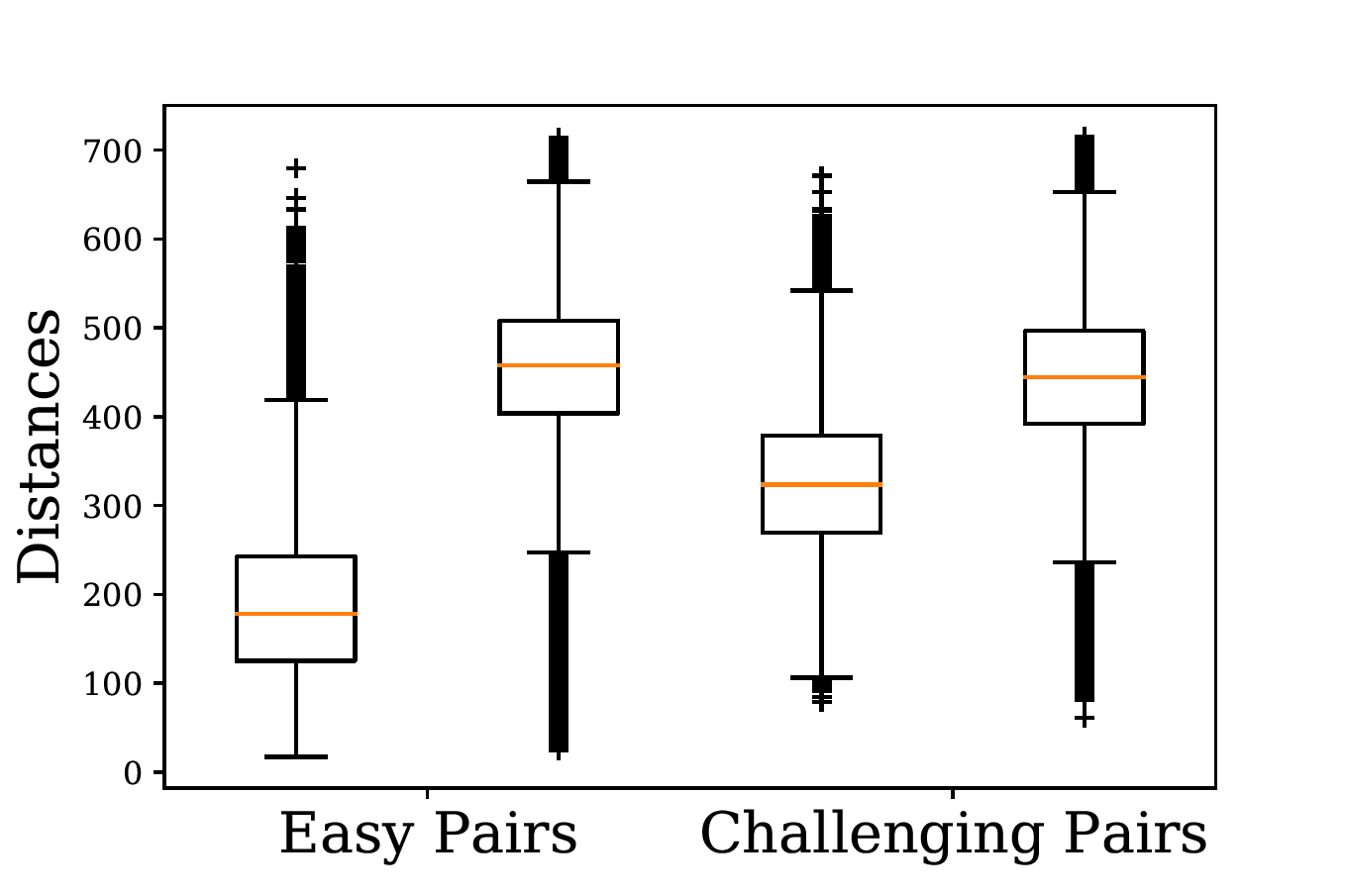
Figure 5: Boxplots of distances between SIFT descriptors for (left to right) Reichstag, Brandenburg Gate and Temple Nara scenes. We split datasets into easy and challenging pairs according to OpenCV matching algorithm score (image pairs with less than $50\%$ correctly matched descriptors are considered challenging, the others are easy pairs). For each scene we then draw the boxplots of distances between descriptors of matching keypoints and non-matching keypoints grouped by easy and challenging pairs, respectively.

6 Discussion and outlook

Intuitions on the separation rate

Let us provide some explanations that should help to gain intuition on the conditions on $\bar{\kappa}_{\textup{in-in}}$ and $\bar{\kappa}_{\textup{in-out}}$ obtained in our main theorems. More precisely, we will explain in this paragraph where the right hand side of (9) comes from. Consider the simpler problem in which we wish to test the hypothesis $H_{0}:\boldsymbol{\mu}=0$ against $H_{1}:\boldsymbol{\mu}\neq 0$ based on the observation $\boldsymbol{Y}$ drawn from the Gaussian distribution $\mathcal{N}_{d}(\boldsymbol{\mu},\sigma^{2}\mathbf{I}_{d})$. This problem has a tight link with the considered problem of matching, since one can think of $\boldsymbol{Y}$ as the difference $\boldsymbol{X}_{i}-\boldsymbol{X}^{\text{\tt\#}}_{j}$. We are interested in checking whether the pair $(i,j)$ is such that $j=\pi^{*}(i)$, that is whether $H_{0}$ is true.

Using the standard bounds on the tails of the chi-squared distribution (Lemma 1), one can check that under $H_{0}$, the random vector $\boldsymbol{Y}$ lies with probability $\geq 1-\alpha$ in the ring $\mathfrak{R}_{0}=B(0,\sigma\sqrt{d+r_{2}})\setminus B(0,\sigma\sqrt{d-r_{1}})$ where

$$r_{1}=2\sqrt{d\log(1/\alpha)}\qquad\text{and}\qquad r_{2}=2\sqrt{d\log(1/\alpha)}+2\log(1/\alpha).$$ (22)

Similarly, considering the approximation $\|\boldsymbol{Y}\|_{2}^{2}\approx\|\boldsymbol{\mu}\|_{2}^{2}+\sigma^{2}\|\boldsymbol{\xi}\|_{2}^{2}$ where $\boldsymbol{\xi}$ is a standard Gaussian vector, we can check that under $H_{1}$, the random vector $\boldsymbol{Y}$ lies with probability $\geq 1-\alpha$ in the ring $\mathfrak{R}_{1}=B(0,\sigma\sqrt{\|\boldsymbol{\mu}/\sigma\|_{2}^{2}+d+r_{2}})\setminus B(0,\sigma\sqrt{\|\boldsymbol{\mu}/\sigma\|_{2}^{2}+d-r_{1}})$.

If the two rings $\mathfrak{R}_{0}$ and $\mathfrak{R}_{1}$ are disjoint, it is possible to decide between $H_{0}$ and $H_{1}$ by checking whether $\boldsymbol{Y}$ belongs to $\mathfrak{R}_{0}$ or not. This condition of disjointness is equivalent to

$$\|\boldsymbol{\mu}/\sigma\|_{2}^{2}+d-r_{1}>{d+r_{2}}.$$ (23)

This leads to

$$\|\boldsymbol{\mu}/\sigma\|_{2}>\sqrt{r_{1}+r_{2}} =\big{(}4\sqrt{d\log(1/\alpha)}+2\log(1/\alpha)\big{)}^{1/2}$$ (24)

$$\asymp\big{(}d\log(1/\alpha)\big{)}^{1/4}\vee\log^{1/2}(1/\alpha).$$ (25)

The right hand side of the last display is of the same order as the right hand side of the (9), for small values of $nm$. The fact that for large values of $nm$ there is a logarithmic deterioration, due to the fact that we have to test a large number of hypotheses $H_{0,i,j}:\theta_{\pi^{*}(i)}={\theta}^{\text{\tt\#}}_{j}$, $(i,j)\in[n]\times[m]$, is quite common in probability and statistics.

Other noise distributions

The results of this paper can be extended to sub-Gaussian distributions without any change in the rates. The extension to sub-exponential distributions seems also possible to do using the methodology employed in this paper, but will most likely lead to higher-order polylogarithmic terms.

Finally, considering heavy tailed distributions such as the multivariate Student distribution might have stronger impact on the rate. Studying this impact is out of scope of the present work.

Outlier detection

The results presented in previous sections provide conditions under which the objective mapping is identified with high probability. This automatically implies that the outliers are correctly identified. However, the task of outlier detection is arguably simpler than that of estimation/detection of $\pi^{*}$. Therefore, one may wonder whether this task can be accomplished under weaker assumptions than those required in the theorems stated in this paper. Somewhat surprisingly, it turns out that this is not the case unless we require the outliers to be very far away from the inliers.

Indeed, on the one hand, if the normalized distance between the outliers and the inliers is not larger than $O(d^{1/2})$, it follows from the counter-example constructed in the proof of Theorem 3 that it is impossible to identify the outliers using a distance based $M$-estimator. Moreover, this impossibility holds for every estimator $\hat{\pi}$ of the set of outliers, as shown in Theorem 4.

On the other hand, suitably adapting the arguments of the proof of Theorem 5, one can prove that if the inlier-outlier distance is larger than a threshold of order $\sqrt{d}\exp(cn)$ for some $c>0$, the LSL recovers the true set of outliers.

Estimation of $\pi^{*}$ instead of detection

An interesting yet challenging problem is that of assessing the minimax risk of estimation of $\pi^{*}$ when the error is measured, for instance, by means of the Hamming loss $\ell_{\textup{Hamming}}(\hat{\pi};\pi^{*})=\#\{i\in[n]:\hat{\pi}(i)\neq\pi^{*}(i)\}$. It is relevant to study this problem in a setting where consistent detection of $\pi^{*}$ (i.e., Hamming loss equal to zero) is impossible, that is when the separation conditions are violated but some weaker assumptions are satisfied. On a related note, one may look for conditions on the normalized separation distances which ensure the existence of an estimator $\hat{\pi}$ such that $\mathbf{P}(\ell_{\textup{Hamming}}(\hat{\pi};\pi^{*})\leq\tau n)\geq 1-\alpha$. This means that with probability $\geq 1-\alpha$ the fraction of mismatched vectors of the estimated map $\hat{\pi}$ is less than $\tau$, for $\tau\in(0,1)$. Note that these problems are not studied even in the simpler outlier-free framework.

7 Conclusion

We have investigated the detection regions in the problem of detection of the matching map between two sequences of noisy vectors. We have shown that the presence of outliers in one of the two sequences has a strong negative impact on the detection region. Interestingly, this negative impact is mitigated in the regime of mild heteroscedasticity, i.e., when noise variances are of the same order of magnitude. In the extremely favorable case of homoscedastic noise (all variances are equal), the presence of outliers does not make the problem any harder, provided that the outliers are at least as different from inliers as two distinct inliers are different one another. Precise forms of the detection region in these different cases can be found in Table 1. The results of the numerical experiments conducted on both synthetic and real data confirm our findings and, furthermore, show the good behaviour of the LSL estimator in terms of its robustness to noise and to outliers, not only in the problem of detection but also in the problem of estimation. In the future, we plan to investigate the case when both sequences contain outliers and to obtain theoretical guarantees on the estimation error measured by the Hamming distance.

Appendix A Postponed proofs

In this appendix we have collected the proofs of the theorems presented in the main text of the paper, as well as some technical definitions used in the proofs. First, denote

$$\sigma_{i,j}^{2}=\sigma_{i}^{2}+\sigma^{\text{\tt\#}2}_{j}\qquad\text{and}\qquad\kappa_{i,j}=\frac{\|\theta_{i}-{\theta}^{\text{\tt\#}}_{j}\|}{\sigma_{i,j}}$$ (26)

for any pair of indices $(i,j)$ with $i\in[n]$ and $j\in[m]$. We will also use the notation

$$\bar{\kappa}=\min(\bar{\kappa}_{\textup{in-in}},\bar{\kappa}_{\textup{in-out}}).$$ (27)

Second, we define the random variables $\zeta_{1}$ and $\zeta_{2}$ as follows

$$\zeta_{1}=\max_{i\neq j}\frac{\big{|}(\theta_{i}-{\theta}^{\text{\tt\#}}_{j})^{\top}(\sigma_{i}\xi_{i}-\sigma^{\text{\tt\#}}_{j}\xi^{\text{\tt\#}}_{j})\big{|}}{\|\theta_{i}-{\theta}^{\text{\tt\#}}_{j}\|\sigma_{i,j}},\quad\zeta_{2}=d^{-1/2}\max_{i,j}\bigg{|}\frac{\big{\|}\sigma_{i}\xi_{i}-\sigma^{\text{\tt\#}}_{j}\xi^{\text{\tt\#}}_{j}\big{\|}^{2}}{\sigma_{i,j}^{2}}-d\bigg{|}.$$ (28)

It can be easily noticed that $\zeta_{1}=\max_{i\neq j}|\zeta_{i,j}|$, where $\zeta_{i,j}$ are standard Gaussian random variables. As for $\zeta_{2}$, it can be seen that $\zeta_{2}=d^{-1/2}\max_{i,j}|\eta_{i,j}|$, where $\eta_{i,j}$ are centered $\chi^{2}$ random variables with $d$ degrees of freedom, i.e. $\eta_{i,j}\stackrel{{\scriptstyle\mathscr{D}}}{{=}}\chi^{2}_{d}-d$.

In addition, one can infer from (1) that for every $i\in[n]$ and every $j\in[m]$, we have

$$\|X_{i}-X^{\text{\tt\#}}_{j}\|^{2} \leq\|\theta_{i}-{\theta}^{\text{\tt\#}}_{j}\|^{2}+\sigma_{i,j}^{2}(d+\sqrt{d}\,\zeta_{2})+2\zeta_{1}\|\theta_{i}-{\theta}^{\text{\tt\#}}_{j}\|\sigma_{i,j}$$ (29)

$$=\sigma_{i,j}^{2}\big{(}\kappa_{i,j}^{2}+d+\sqrt{d}\,\zeta_{2}+2\zeta_{1}\kappa_{i,j}\big{)},$$ (30)

$$\|X_{i}-X^{\text{\tt\#}}_{j}\|^{2} \geq\|\theta_{i}-{\theta}^{\text{\tt\#}}_{j}\|^{2}+\sigma_{i,j}^{2}(d-\sqrt{d}\,\zeta_{2})-2\zeta_{1}\|\theta_{i}-{\theta}^{\text{\tt\#}}_{j}\|\sigma_{i,j}$$ (31)

$$=\sigma_{i,j}^{2}\big{(}\kappa_{i,j}^{2}+d-\sqrt{d}\,\zeta_{2}-2\zeta_{1}\kappa_{i,j}\big{)}.$$ (32)

The concentration of the centered and normalized $\chi^{2}$ random variable, such as $\zeta_{2}$, is described in the following lemma.

Lemma 1 (Laurent and Massart [26], Eq. (4.3) and (4.4)).

If $Y$ is drawn from the chi-squared distribution $\chi^{2}(D)$, where $D\in\mathbb{N}^{*}$, then, for every $x>0$,

$$\begin{cases}\ \mathbf{P}\big{(}Y-D\leq-2\sqrt{Dx}\big{)}\leq e^{-x},\phantom{\Big{(})}\\ \ \mathbf{P}\big{(}Y-D\geq 2\sqrt{Dx}+2x\big{)}\leq e^{-x}.\phantom{\Big{(})}\end{cases}$$ (33)

As a consequence, for every $y>0$, $\mathbf{P}\big{(}D^{-1/2}|Y-D|\geq y\big{)}\leq 2\exp\big{\{}-\textstyle\frac{1}{8}y(y\wedge\sqrt{D})\big{\}}$. Or, equivalently, for any $\alpha\in(0,1)$, we have

$$\mathbf{P}\bigg{(}D^{-1/2}|Y-D|\leq 2\sqrt{\log(2/\alpha)}+\frac{2\log(2/\alpha)}{\sqrt{D}}\bigg{)}\geq 1-\alpha.$$ (34)

A.1 Proof of Theorem 1

We prove the upper bound for $\bar{\kappa}$ in the presence of outliers. Without loss of generality we can assume that $\pi^{*}(i)=i,~{}~{}\forall i\in[n]$. We wish to bound the probability of the event $\Omega=\{\hat{\pi}\neq\pi^{*}\}$, where $\hat{\pi}=\bar{\pi}^{\text{LSNS}}$. It is evident that

$$\Omega\subset\bigcup_{\pi\neq\pi^{*}}\Omega_{\pi},$$ (35)

where the union is taken over all possible injective mappings $\pi:[n]\to[m]$ and

$$\Omega_{\pi} =\bigg{\{}\sum_{i=1}^{n}\frac{\|X_{i}-X^{\text{\tt\#}}_{i}\|^{2}}{2\sigma_{i}^{2}}\geq\sum_{i=1}^{n}\frac{\|X_{i}-X^{\text{\tt\#}}_{\pi(i)}\|^{2}}{\sigma_{i}^{2}+(\sigma^{\text{\tt\#}}_{\pi(i)})^{2}}\bigg{\}}.$$ (36)

One easily checks that the following inclusion holds:

$$\Omega_{\pi}\subset\bigcup_{i=1}^{n}\bigcup_{j\in[m]\setminus\{i\}}\bigg{\{}\frac{\|X_{i}-X^{\text{\tt\#}}_{i}\|^{2}}{2\sigma_{i}^{2}}\geq\frac{\|X_{i}-X^{\text{\tt\#}}_{j}\|^{2}}{\sigma_{i}^{2}+(\sigma^{\text{\tt\#}}_{j})^{2}}\bigg{\}}.$$ (37)

Since $\pi^{*}(i)=i$ for every $i\in[n]$, $\kappa_{i,i}=0$ (see the definition in (26)) and, in view of (30),

$$\|X_{i}-X^{\text{\tt\#}}_{i}\|^{2}\leq 2\sigma_{i}^{2}(d+\sqrt{d}\,\zeta_{2}).$$ (38)

Similarly, for every $j\in[m]$ and $j\neq i$, in view of (32),

$$\|X_{i}-X^{\text{\tt\#}}_{j}\|^{2} \geq\sigma_{i,j}^{2}(\kappa_{i,j}^{2}+d-\sqrt{d}\,\zeta_{2}-2\kappa_{i,j}\zeta_{1}).$$ (39)

Recall that $\bar{\kappa}$ defined in (27), is the smallest normalized distance $\kappa_{i,j}$. Therefore, on the event $\Omega_{1}=\{\bar{\kappa}\geq\zeta_{1}\}$, the previous display implies that

$$\frac{\|X_{i}-X^{\text{\tt\#}}_{j}\|^{2}}{\sigma_{i,j}^{2}}\geq\bar{\kappa}^{2}-2\bar{\kappa}\zeta_{1}+d-\sqrt{d}\,\zeta_{2}.$$ (40)

Hence, combining obtained bounds (38) and (40) we get that

$$\bigg{\{}\frac{\|X_{i}-X^{\text{\tt\#}}_{i}\|^{2}}{2\sigma_{i}^{2}}\geq\frac{\|X_{i}-X^{\text{\tt\#}}_{j}\|^{2}}{\sigma_{i}^{2}+(\sigma^{\text{\tt\#}}_{j})^{2}}\bigg{\}}\cap\Omega_{1} \subset\Big{\{}d+\sqrt{d}\,\zeta_{2}\geq\bar{\kappa}^{2}-2\bar{\kappa}\zeta_{1}+d-\sqrt{d}\,\zeta_{2}\Big{\}}$$ (41)

$$=\Big{\{}2\sqrt{d}\,\zeta_{2}+2\bar{\kappa}\,\zeta_{1}\geq\bar{\kappa}^{2}\Big{\}}.$$ (42)

Note that the event on the right hand side of the last display is independent of the pair $(i,j)$. This implies that

$$\Omega\cap\Omega_{1} \stackrel{{\scriptstyle\textup{by \eqref{omega1}}}}{{\subset}}\bigg{(}\bigcup_{\pi\neq\pi^{*}}\Omega_{\pi}\bigg{)}\cap\Omega_{1}$$ (43)

$$\stackrel{{\scriptstyle\textup{by \eqref{omega2}}}}{{\subset}}\bigg{(}\bigcup_{i=1}^{n}\bigcup_{j\in[m]\setminus\{i\}}\bigg{\{}\frac{\|X_{i}-X^{\text{\tt\#}}_{i}\|^{2}}{2\sigma_{i}^{2}}\geq\frac{\|X_{i}-X^{\text{\tt\#}}_{j}\|^{2}}{\sigma_{i}^{2}+(\sigma^{\text{\tt\#}}_{j})^{2}}\bigg{\}}\bigg{)}\cap\Omega_{1}$$ (44)

$$\stackrel{{\scriptstyle\hphantom{\textup{by \eqref{omega3}}}}}{{\subset}}\bigcup_{i=1}^{n}\bigcup_{j\in[m]\setminus\{i\}}\bigg{(}\bigg{\{}\frac{\|X_{i}-X^{\text{\tt\#}}_{i}\|^{2}}{2\sigma_{i}^{2}}\geq\frac{\|X_{i}-X^{\text{\tt\#}}_{j}\|^{2}}{\sigma_{i}^{2}+(\sigma^{\text{\tt\#}}_{j})^{2}}\bigg{\}}\cap\Omega_{1}\bigg{)}$$ (45)

$$\stackrel{{\scriptstyle\textup{by \eqref{omega3}}}}{{\subset}}\Big{\{}2\sqrt{d}\,\zeta_{2}+2\bar{\kappa}\,\zeta_{1}\geq\bar{\kappa}^{2}\Big{\}}.$$ (46)

Using (46) we can show that

$$\mathbf{P}(\Omega) \leq\mathbf{P}(\Omega_{1}^{\complement})+\mathbf{P}\big{(}\Omega\cap\Omega_{1}\big{)}$$ (47)

$$\leq\mathbf{P}\big{(}\zeta_{1}\geq\bar{\kappa}\big{)}+\mathbf{P}(2\sqrt{d}\zeta_{2}+2\bar{\kappa}\zeta_{1}\geq\bar{\kappa}^{2})$$ (48)

$$\leq\mathbf{P}\big{(}\zeta_{1}\geq\bar{\kappa}\big{)}+\mathbf{P}\big{(}\zeta_{1}\geq{\textstyle\frac{1}{4}}\bar{\kappa}\big{)}+\mathbf{P}\Big{(}2\sqrt{d}\zeta_{2}+2\bar{\kappa}\zeta_{1}\geq\bar{\kappa}^{2};\zeta_{1}<{\textstyle\frac{1}{4}}\bar{\kappa}\Big{)}$$ (49)

$$\leq 2\mathbf{P}\big{(}\zeta_{1}\geq{\textstyle\frac{1}{4}}\,{\bar{\kappa}}\big{)}+\mathbf{P}\bigg{(}\zeta_{2}\geq\frac{\bar{\kappa}^{2}}{4\sqrt{d}}\bigg{)}.$$ (50)

For suitably chosen standard Gaussian random variables $\zeta_{i,j}$ it holds that $\zeta_{1}=\max_{i\not=j}|\zeta_{i,j}|$. Therefore, using the tail bound for the standard Gaussian distribution and the union bound, we get

$$\mathbf{P}\Big{(}\zeta_{1}\geq{\textstyle\frac{1}{4}}\bar{\kappa}\Big{)} \leq\sum_{i\not=j}\mathbf{P}\Big{(}|\zeta_{i,j}|\geq\textstyle\frac{1}{4}\bar{\kappa}\Big{)}\leq 2nm\,e^{-\bar{\kappa}^{2}/32}.$$ (51)

To complete the proof, it remains to upper bound the second term in the right hand side of (50), i.e., to evaluate the tail of the random variable $\zeta_{2}$. To this end, we use the concentration result stated in Lemma 1 with $y=\frac{\bar{\kappa}^{2}}{4\sqrt{d}}$, combined with the union bound and simple algebra. This yields

$$\mathbf{P}\Big{(}\zeta_{2}\geq\frac{\bar{\kappa}^{2}}{4\sqrt{d}}\Big{)} \leq 2nm\exp\Big{\{}-\frac{1}{8}\cdot\frac{\bar{\kappa}^{2}}{4\sqrt{d}}\Big{(}\frac{\bar{\kappa}^{2}}{4\sqrt{d}}\wedge\sqrt{d}\Big{)}\Big{\}}$$ (52)

$$=2nm\exp\Big{\{}-\frac{(\bar{\kappa}/16)^{2}}{d}(2\bar{\kappa}^{2}\wedge 8d)\Big{\}},$$ (53)

where the $nm$ factor in front of the exponent comes from the union bound for all $nm$ pairs $(i,j)$ from the definition of $\zeta_{2}$, while the exponent is a direct application of Lemma 1. Finally, using inequalities (50)-(53), we get that whenever

$$\bar{\kappa}\geq 4\Big{(}\sqrt{2\log(8nm/\alpha)}\vee\big{(}d\log(4nm/\alpha)\big{)}^{1/4}\Big{)},$$ (54)

the probability of incorrect matching is at most $\alpha$. Thus, we have formally showed that if (54) holds then $\mathbf{P}(\hat{\pi}\neq\pi^{*})=\mathbf{P}(\Omega)\leq\alpha,$ as desired.

A.2 Proof of Theorem 2

We prove the upper bound for $\bar{\kappa}=\min(\bar{\kappa}_{\textup{in-in}},\bar{\kappa}_{\textup{in-out}})$ in the presence of outliers and in the case of unknown noise variance. We wish to bound the probability of the event $\Omega=\{\hat{\pi}\neq\pi^{*}\}$, where $\hat{\pi}=\hat{\pi}^{\textup{LSL}}$ and $\pi^{*}(i)=i$ for all $i\in[n]$. It is evident that

$$\Omega\in\bigcup_{\pi\neq\pi^{*}}\Omega_{\pi},$$ (55)

where

$$\Omega_{\pi} =\Big{\{}\sum_{i=1}^{n}\log\|X_{i}-X^{\text{\tt\#}}_{i}\|^{2}\geq\sum_{i=1}^{n}\log\|X_{i}-X^{\text{\tt\#}}_{\pi(i)}\|^{2}\Big{\}}$$ (56)

$$\subset\bigcup_{i=1}^{n}\bigcup_{j\in[m]\setminus\{i\}}\Big{\{}\log\|X_{i}-X^{\text{\tt\#}}_{i}\|^{2}\geq\log\|X_{i}-X^{\text{\tt\#}}_{j}\|^{2}\Big{\}}$$ (57)

Recall that $\bar{\kappa}=\min(\bar{\kappa}_{\textup{in-in}},\bar{\kappa}_{\textup{in-out}})$. On the event $\Omega_{1}=\{\bar{\kappa}\geq\zeta_{1}\}$, from equation (32), we get

$$\frac{\|X_{i}-X^{\text{\tt\#}}_{j}\|^{2}}{\sigma_{i,j}^{2}}\geq\bar{\kappa}^{2}-2\zeta_{1}\bar{\kappa}+d-\sqrt{d}\,\zeta_{2}.$$ (58)

Note that the expression on the right hand side of the last display is independent of the pair $(i,j)$. This implies that

$$\Omega\cap\Omega_{1} {\subset}\bigg{(}\bigcup_{\pi\neq\pi^{*}}\Omega_{\pi}\bigg{)}\cap\Omega_{1}$$ [by (55)]

$${\subset}\bigg{(}\bigcup_{i=1}^{n}\bigcup_{j\in[m]\setminus\{i\}}\bigg{\{}\log\|X_{i}-X^{\text{\tt\#}}_{i}\|^{2}\geq\log\|X_{i}-X^{\text{\tt\#}}_{j}\|^{2}\bigg{\}}\bigg{)}\cap\Omega_{1}$$ [by (57)]

$${\subset}\bigcup_{i=1}^{n}\bigcup_{j\in[m]\setminus\{i\}}\bigg{(}\bigg{\{}\|X_{i}-X^{\text{\tt\#}}_{i}\|^{2}\geq\|X_{i}-X^{\text{\tt\#}}_{j}\|^{2}\bigg{\}}\cap\Omega_{1}\bigg{)}$$ (59)

$${\subset}\Big{\{}2\sigma_{i}^{2}(d+\sqrt{d}\zeta_{2})\geq\sigma_{i,j}^{2}(\bar{\kappa}^{2}-2\zeta_{1}\bar{\kappa}+d-\sqrt{d}\,\zeta_{2})\Big{\}}$$ [by (30),(58)]

$${\subset}\Big{\{}2(d+\sqrt{d}\zeta_{2})\geq\bar{\kappa}^{2}-2\zeta_{1}\bar{\kappa}+d-\sqrt{d}\,\zeta_{2}\Big{\}}, \sigma_{i}\leq\sigma_{i,j}$$ [since ]

$${\subset}\Big{\{}3\sqrt{d}\,\zeta_{2}+2\zeta_{1}\bar{\kappa}\geq\bar{\kappa}^{2}-d\Big{\}}.$$ (60)

We can bound the probability of incorrect matching $\mathbf{P}(\Omega)$ using the relationship obtained in (60)

$$\mathbf{P}(\Omega) \leq\mathbf{P}(\Omega_{1}^{\complement})+\mathbf{P}(\Omega\cap\Omega_{1})$$ (61)

$$\leq\mathbf{P}(\zeta_{1}\geq\bar{\kappa})+\mathbf{P}\big{(}3\sqrt{d}\,\zeta_{2}+2\zeta_{1}\bar{\kappa}\geq\bar{\kappa}^{2}-d\big{)}.$$ (62)

From the last inequality, we infer that

$$\mathbf{P}(\Omega) \leq\mathbf{P}(\zeta_{1}\geq\bar{\kappa})+\mathbf{P}\Big{(}\zeta_{1}\geq{\textstyle\frac{1}{4}}{\bar{\kappa}}\Big{)}+\mathbf{P}\Big{(}3\sqrt{d}\,\zeta_{2}+2\zeta_{1}\bar{\kappa}\geq\bar{\kappa}^{2}-d\,;\,\zeta_{1}<{\textstyle\frac{1}{4}}\bar{\kappa}\Big{)}$$ (63)

$$\leq 2\mathbf{P}\Big{(}\zeta_{1}\geq{\textstyle\frac{1}{4}}{\bar{\kappa}}\Big{)}+\mathbf{P}\Big{(}3\sqrt{d}\,\zeta_{2}\geq{\textstyle\frac{1}{2}\bar{\kappa}^{2}}-d\Big{)}$$ (64)

$$\leq 2\mathbf{P}\Big{(}\zeta_{1}\geq{\textstyle\frac{1}{4}}{\bar{\kappa}}\Big{)}+\mathbf{P}\Big{(}\zeta_{2}\geq\frac{\bar{\kappa}^{2}-2d}{6\sqrt{d}}\Big{)}.$$ (65)

As mentioned in the beginning of the section, for suitably chosen standard Gaussian random variables $\zeta_{i,j}$ it holds that $\zeta_{1}=\max_{i\not=j}|\zeta_{i,j}|$. Therefore, using the tail bound for the standard Gaussian distribution and the union bound, we get

$$\mathbf{P}\Big{(}\zeta_{1}\geq{\textstyle\frac{1}{4}}\bar{\kappa}\Big{)} \leq\sum_{i\not=j}\mathbf{P}\Big{(}|\zeta_{i,j}|\geq\textstyle\frac{1}{4}\bar{\kappa}\Big{)}\leq 2nm\,e^{-\bar{\kappa}^{2}/32}\leq\alpha/4.$$ (66)

To complete the proof, it remains to upper bound the second term in the right hand side of (65), i.e., to evaluate the tail of the random variable $\zeta_{2}$. Using Lemma 1 with $y=(\bar{\kappa}^{2}-2d)/(6\sqrt{d})$—which is positive under the conditions of the theorem—combined with the union bound, we arrive at

$$\mathbf{P}(\zeta_{2}\geq y) \leq 2nm\exp\Big{\{}-\frac{1}{8}y(y\wedge\sqrt{d})\Big{\}}$$ (67)

$$=2nm\bigg{(}\exp\Big{\{}-\frac{1}{8}y^{2}\Big{\}}\vee\exp\Big{\{}-\frac{1}{8}y\sqrt{d}\Big{\}}\bigg{)}.$$ (68)

One easily checks that the last expression is smaller than $\alpha/2$ if and only if

$$y^{2}\geq 8\log(4nm/\alpha)\qquad\text{and}\qquad y\sqrt{d}\geq 8\log(4nm/\alpha)$$ (69)

which is equivalent to

$$y\geq\big{(}2\sqrt{2\log(4nm/\alpha)}\big{)}\vee\big{(}(8/\sqrt{d})\log(4nm/\alpha)\big{)}.$$ (70)

Replacing $y=(\bar{\kappa}^{2}-2d)/(6\sqrt{d})$, the last inequality becomes

$$\bar{\kappa}^{2}\geq 2d+\big{(}12\sqrt{2d\log(4nm/\alpha)}\big{)}\vee\big{(}48\log(4nm/\alpha)\big{)}.$$ (71)

Combining the inequality from the last display with the bound derived from (66) we get that all these bounds are satisfied whenever

$$\bar{\kappa}\geq\sqrt{2d}+4\bigg{\{}\bigg{(}2d\log\frac{4nm}{\alpha}\bigg{)}^{1/4}\vee\bigg{(}3\log\frac{8nm}{\alpha}\bigg{)}^{1/2}\bigg{\}}.$$ (72)

Therefore, under this condition on $\bar{\kappa}$, the probability of the incorrect matching is at most $\alpha$, i.e. $\mathbf{P}(\hat{\pi}\neq\pi^{*})=\mathbf{P}(\Omega)\leq\alpha$.

A.3 Proof of Theorem 3

First we fix $m=n+1$ and $\pi^{*}(i)=i$ for all $i\in[n]$, where $\pi^{*}$ is the correct matching. Let $\sigma^{\text{\tt\#}}_{1}=1$ and $\sigma^{\text{\tt\#}}_{i+1}=\alpha^{i}$ for all $i\in[n]$, where $\alpha\ll 1$. Then let’s take $\pi(i)=i+1$ for all $i\in[n]$. Let $L(\pi)$ be the vector of distances $\|X_{i}-X^{\text{\tt\#}}_{\pi(i)}\|$ for a matching scheme $\pi$

$$L(\pi)=\begin{bmatrix}\|X_{1}-X^{\text{\tt\#}}_{\pi(1)}\|\\ \|X_{2}-X^{\text{\tt\#}}_{\pi(2)}\|\\ \cdots\\ \|X_{n}-X^{\text{\tt\#}}_{\pi(n)}\|\end{bmatrix}.$$ (73)

The next lemma shows that the event $L(\bar{\pi})<L(\pi^{*})$ (coordinate-wise) occurs with probability at least $1/4$.

Lemma 2.

Let $n\geq 4$, $d\geq 422\log(4n)$ and ${\theta}^{\text{\tt\#}}_{1}=(1;0;\ldots;0)^{\top}$. Assume that $\pi^{*}(i)=i$, $\sigma^{\text{\tt\#}}_{i}=2^{-(i-1)}$ and ${\theta}^{\text{\tt\#}}_{i+1}={\theta}^{\text{\tt\#}}_{i}+2^{-(i+1)}\sqrt{d}\,{\theta}^{\text{\tt\#}}_{1}$ for all $i\in[n+1]$. Then $L(\pi^{*})>L(\bar{\pi})$ with probability greater than $1/4$, where $\bar{\pi}$ is the injection defined by $\bar{\pi}(i)=i+1$. Furthermore, for these values $(\boldsymbol{\theta}^{\text{\tt\#}},\boldsymbol{\sigma}^{\text{\tt\#}},\pi^{*})$, we have $\kappa_{\textup{in-in}}=\kappa_{\textup{in-out}}=\sqrt{d/20}$.

• Let us denote

  $$\bar{\kappa}_{i}\triangleq\frac{\|{\theta}^{\text{\tt\#}}_{\pi(i)}-\theta_{i}\|}{\sqrt{\sigma_{i}^{2}+\sigma^{\text{\tt\#}2}_{\bar{\pi}(i)}}}=\sqrt{d/20},\qquad\text{for all }i\in[n].$$ (74)

  Recall that $\sigma_{i,j}^{2}=\sigma_{i}^{2}+\sigma^{\text{\tt\#}2}_{j}$ and write

  $$L_{i}(\pi)=\|X_{i}-X^{\text{\tt\#}}_{\pi(i)}\|^{2} =\|\theta_{i}-{\theta}^{\text{\tt\#}}_{\pi(i)}+\zeta_{i}\sigma_{i,\pi(i)}\|^{2},$$ (75)

  where $\zeta_{i}\sim\mathcal{N}(0,I_{d})$. Notice that $L_{i}(\pi^{*})=2\sigma_{i}^{2}\|\zeta_{i}\|^{2}$ for all $i\in[n]$. Similarly, the expression from the last display for $\bar{\pi}$ reads as

  $$L_{i}(\bar{\pi})=\|\zeta_{i}\sigma_{i,\bar{\pi}(i)}\|^{2}\Big{(}1+\frac{\bar{\kappa}_{i}^{2}}{\|\zeta_{i}\|^{2}}\Big{)}+{2\sigma_{i,\bar{\pi}(i)}\zeta_{i}^{\top}(\theta_{i}-{\theta}^{\text{\tt\#}}_{\bar{\pi}(i)})}.$$ (76)

  Plugging in the values of $\boldsymbol{\sigma}^{\text{\tt\#}}$ with $\alpha=1/2$ and $\bar{\pi}(i)=i+1$ we arrive at

  $$L_{i}(\pi^{*})=2^{3-2i}\|\zeta_{i}\|^{2},\qquad L_{i}(\bar{\pi})=\frac{5}{2^{2i}}\|\bar{\zeta}_{i}\|^{2}\Big{(}1+\frac{\bar{\kappa}_{i}^{2}}{\|\bar{\zeta}_{i}\|^{2}}\Big{)}+\frac{\sqrt{5}}{2^{i-1}}\bar{\zeta}_{i}^{\top}(\theta_{i}-{\theta}^{\text{\tt\#}}_{i+1}),$$ (77)

  where in the second expression we write $\bar{\zeta}_{i}$ instead of $\zeta_{i}$ to indicate that these random variables are different, though both are standard normal $d$-dimensional vectors. We first replace the second term of $L_{i}(\bar{\pi})$ with its upper bound that holds with probability of at least $1/4$. It is evident that the random variable $Z\triangleq{2\sigma_{i,\bar{\pi}(i)}\zeta_{i}^{\top}(\theta_{i}-{\theta}^{\text{\tt\#}}_{\bar{\pi}(i)})}$ is Gaussian with standard deviation $\sigma\triangleq 2\sigma_{i,\bar{\pi}(i)}\|\theta_{i}-{\theta}^{\text{\tt\#}}_{\bar{\pi}(i)}\|=2\sigma_{i,\bar{\pi}(i)}^{2}\bar{\kappa}_{i}$, therefore

  $$\mathbf{P}(Z\geq\sigma\sqrt{2\log 4})\leq\frac{1}{4}.$$ (78)

  Hence, on the event $\Omega=\{Z\leq 2\sigma_{i,\bar{\pi}(i)}^{2}\bar{\kappa}_{i}\sqrt{2\log 4}\}$ the inequality $L_{i}(\pi^{*})>L_{i}(\bar{\pi})$ holds whenever

  $$\frac{8}{2^{2i}}\|\zeta_{i}\|^{2}>\frac{5}{2^{2i}}\|\bar{\zeta}_{i}\|^{2}\Big{(}1+\frac{\bar{\kappa}_{i}^{2}}{\|\bar{\zeta}_{i}\|^{2}}\Big{)}+\frac{5}{2^{2i}}\bar{\kappa}_{i}\sqrt{8\log 4},$$

  $$\frac{8}{5}\|\zeta_{i}\|^{2}-\|\bar{\zeta}_{i}\|^{2}>\bar{\kappa}_{i}^{2}+2\bar{\kappa}_{i}\sqrt{2\log 4}.$$ (79)

  Notice that the left hand side of (79) is a weighted difference of two centered and normalized $\chi^{2}$ random variables with $d$ degrees of freedom. The concentration inequality for such difference is a direct consequence of Lemma 1. Namely, for $X,Y\sim\chi^{2}_{d}$ the concentration bound for $Z=\alpha X-\beta Y$ with arbitrary $\alpha,\beta\in\mathbb{R}$ reads as

  $$\mathbf{P}(Z\geq(\alpha-\beta)d-2\sqrt{dx}(\alpha+\beta)-2\beta x)\geq 1-2e^{-x}.$$ (80)

  It is easy to verify that given $n\geq 4,d\geq 422\log(4n)$ and $\bar{\kappa}_{i}\leq\sqrt{d/20}$, then

  $$\bar{\kappa}_{i}^{2}+2\bar{\kappa}_{i}\sqrt{2\log 4}\leq\frac{3}{5}d-\frac{26}{5}\sqrt{d\log(4n)}-2\log(4n),$$ (81)

  where the right hand side is the quantile of $Z$ with $x=\log(4n)$. Combining the inequality from the last display with (79) we get that on the event $\Omega$ we have

  $$\mathbf{P}(L_{i}(\pi^{*})>L_{i}(\bar{\pi}))\geq 1-\frac{1}{2n}.$$ (82)

  Recall that $\mathbf{P}(\Omega)\geq 3/4$, then using the union bound for events $\Omega$ and $\{L_{i}(\pi^{*})>L_{i}(\bar{\pi})\}$ all $i\in[n]$ we arrive at $\mathbf{P}(L(\pi^{*})>L(\bar{\pi}))>1/4$. This completes the proof of Lemma 2.

Therefore, using the result of Lemma 2 and applying any non-decreasing function $\rho(\cdot)$ to each of the coordinates of $L(\bar{\pi})$ and $L(\pi^{*})$ yields

$$\sum_{i=1}^{n}\rho_{i}(\|X_{i}-X^{\text{\tt\#}}_{\bar{\pi}(i)}\|)<\sum_{i=1}^{n}\rho_{i}(\|X_{i}-X^{\text{\tt\#}}_{\pi^{*}(i)}\|)$$ (83)

with probability of at least $1/4$. This, in turn, implies that an optimizer will not choose $\pi^{*}$ on this event. Hence, $\mathbf{P}(\bar{\pi}\neq\pi^{*})>\nicefrac{{1}}{{4}}$, concluding the proof of the theorem.

A.4 Proof of Theorem 4

We denote the set of all injective functions $\pi:[n]\to[m]$ as $\mathfrak{I}_{n,m}$. We use the notation $D(\mathbf{P},\mathbf{Q})$ for the Kullback-Leibler (KL) divergence between two probability measures $\mathbf{P}$ and $\mathbf{Q}$ such that $\mathbf{P}$ is absolutely continuous with respect to $\mathbf{Q}$, $\mathbf{P}\ll\mathbf{Q}$. The identity mapping denoted by id is defined as follows: $id(i)=i,\,\,\forall i\in[n]$. It is also assumed that $\pi^{*}=id$.

To establish the general lower bound we use the following lemma:

Lemma 3 (Tsybakov [43], Theorem 2.5).

Assume that for some integer $M\geq 2$ there exist distinct injective functions $\pi_{0},\ldots,\pi_{M}\in\mathfrak{I}_{n,m}$ and mutually absolutely continuous probability measures $\mathbf{Q}_{0},\ldots,\mathbf{Q}_{M}$ defined on a common probability space $(\mathcal{Z},\mathscr{Z})$ such that

$$\frac{1}{M}\sum_{j=1}^{M}D(\mathbf{Q}_{j},\mathbf{Q}_{0})\leq\frac{1}{8}\log M.$$ (84)

Then, for every measurable mapping $\tilde{\pi}:\mathcal{Z}\to\mathfrak{I}_{n,m}$,

$$\max_{j=0,\dots,M}\mathbf{Q}_{j}(\tilde{\pi}\neq\pi_{j})\geq\frac{\sqrt{M}}{\sqrt{M}+1}\Big{(}\frac{3}{4}-\frac{1}{2\sqrt{\log(M)}}\Big{)}.$$ (85)

Since $d\geq 16\log(nm)$ then the rate from Theorem 1 becomes of order $(d\log(nm))^{1/4}$. We show that for $6\kappa\geq(d\log(nm))^{1/4}$ there is indeed a setting where the detection of $\pi^{*}$ fails with probability at least $\nicefrac{{1}}{{4}}$ for any matching map $\tilde{\pi}\in\mathfrak{I}_{n,m}$. To show this we use Lemma 3 with properly chosen family of probability measures described in the following lemma.

Lemma 4 (Collier and Dalalyan [10], Lemma 14).

Let $\varepsilon_{1},\dots,\varepsilon_{m}$ be real numbers defined by

$$\varepsilon_{k}=\sqrt{2/d}\,\kappa\sigma^{\text{\tt\#}}_{k},\quad\forall k\in[m],$$ (86)

and let $\mu$ be the uniform distribution on $\mathcal{E}=\{\pm\varepsilon_{1}\}^{d}\times\dots\times\{\pm\varepsilon_{m}\}^{d}$. Denote by $\mathbf{P}_{\mu,\pi}$ the probability measure on $\mathbb{R}^{d\times m}$ defined by $\mathbf{P}_{\mu,\pi}(A)=\int_{\mathcal{E}}\mathbf{P}_{\boldsymbol{\theta},\pi}(A)\mu(d\boldsymbol{\theta})$. Let $\bar{\Theta}_{\kappa}$ be the set of $\boldsymbol{\theta}^{\text{\tt\#}}$ such that $6\kappa\geq(d\log(nm))^{1/4}$. Assume that $\sigma^{\text{\tt\#}}_{1}\leq\dots\leq\sigma^{\text{\tt\#}}_{m}$ and $\sigma^{\text{\tt\#}2}_{m}/\sigma^{\text{\tt\#}2}_{1}\leq 1+\sqrt{\frac{\log(nm)}{16d}}$. Let $\pi=(k\,\,k^{\prime})$ be the transposition that only permutes $k^{\textup{th}}$ and $k^{\prime\textup{th}}$ observations ($k<k^{\prime})$. Then, the Kullback-Leibler divergence between $\mathbf{P}_{\mu,\pi}$ and $\mathbf{P}_{\mu,id}$ can be bounded as follows

$$D(\mathbf{P}_{\mu,\pi},\mathbf{P}_{\mu,id})\leq\frac{1}{8}\log(m(m-1)/2).$$ (87)

Additionally, $\mu(\mathcal{E}\setminus\bar{\Theta}_{\kappa})\leq(m(m-1)/2)e^{-d/8}$.

Applying Lemma 3 with $M=m(m-1)/2$, $\mathbf{Q}_{0}=\mathbf{P}_{\mu,id}$ and $\{\mathbf{Q}_{j}\}_{j=1,\dots,M}=\{\mathbf{P}_{\mu,\pi_{k,k^{\prime}}}\}_{k\neq k^{\prime}}$ we obtain that for any estimator $\hat{\pi}$

$$\max_{\pi^{*}\in\mathfrak{I}_{n,m}}\sup_{\boldsymbol{\theta}^{\text{\tt\#}}\in\bar{\Theta}_{\kappa}}\mathbf{P}_{\boldsymbol{\theta}^{\text{\tt\#}},\boldsymbol{\sigma}^{\text{\tt\#}},\pi^{*}}(\hat{\pi}\neq\pi^{*}) \geq\max_{\pi^{*}\in\{\textit{id}\}\cup\{\pi_{k,k^{\prime}}\}}\int_{\bar{\Theta}_{\kappa}}\mathbf{P}_{\boldsymbol{\theta}^{\texttt{\#}},\pi^{*}}\big{(}\hat{\pi}\neq\pi^{*}\big{)}\frac{\mu(d\boldsymbol{\theta}^{\texttt{\#}})}{\mu(\bar{\Theta}_{\kappa})}$$ (88)

$$\geq\max_{\pi^{*}\in\{\textit{id}\}\cup\{\pi_{k,k^{\prime}}\}}\mathbf{P}_{\mu,\pi^{*}}\big{(}\hat{\pi}\neq\pi^{*}\big{)}-\mu(\mathcal{E}\setminus\bar{\Theta}_{\kappa})$$ (89)

$$\geq\frac{\sqrt{15}}{\sqrt{15}+1}\Big{(}\frac{3}{4}-\frac{1}{2\sqrt{\log 15}}\Big{)}-\frac{m(m-1)}{2}e^{-d/8},$$ (90)

where in the last inequality we applied the result of Lemma 3 in conjunction with the monotonicity of function $m\mapsto\frac{\sqrt{m}}{1+\sqrt{m}}(3/4-(2\sqrt{\log(m)})^{-1})$. Recall that $m>n\geq 5$ and $d\geq 16\log(nm)$ yielding $\inf_{\hat{\pi}}\mathbf{P}_{\boldsymbol{\theta}^{\text{\tt\#}},\boldsymbol{\sigma}^{\text{\tt\#}},\pi^{*}}(\hat{\pi}\neq\pi^{*})>0.338$, concluding the proof.

A.5 Proof of Theorem 5

To ease notation, we write $\hat{\pi}$ instead of $\hat{\pi}^{\textup{LSL}}_{n,m}$, and, without loss of generality, we assume that $\pi^{*}(i)=i$ for $i\in[n]$. We wish to prove that on an event of probability $\geq 1-\alpha$, for every injective mapping $\pi:[n]\to[m]$, we have $\psi(\pi^{*})\leq\psi(\pi)$, where

$$\psi(\pi)=\sum_{i=1}^{n}\log\|X_{i}-X^{\text{\tt\#}}_{\pi(i)}\|^{2}.$$ (91)

Since the logarithm is an increasing function, this is equivalent to showing that

$$\prod_{i=1}^{n}\|X_{i}-X^{\text{\tt\#}}_{\pi^{*}(i)}\|^{2} <\prod_{i=1}^{n}\|X_{i}-X^{\text{\tt\#}}_{\pi(i)}\|^{2},\quad\text{for every $\pi\neq\pi^{*}$},$$ (92)

which, in turn, is the same as

$$\prod_{i=1}^{n}\frac{\|X_{i}-X^{\text{\tt\#}}_{\pi^{*}(i)}\|^{2}}{\|X_{i}-X^{\text{\tt\#}}_{\pi(i)}\|^{2}}<1,\quad\text{for every $\pi\neq\pi^{*}$}.$$ (93)

In view of (30) and (32), we have

$$\prod_{i=1}^{n}\frac{\|X_{i}-X^{\text{\tt\#}}_{\pi^{*}(i)}\|^{2}}{\|X_{i}-X^{\text{\tt\#}}_{\pi(i)}\|^{2}} \leq\prod_{\begin{subarray}{c}i\in[n]\\ \pi(i)\neq\pi^{*}(i)\end{subarray}}\frac{2\sigma_{i}^{2}(d+\sqrt{d}\,\zeta_{2})}{\sigma_{i,\pi(i)}^{2}\big{(}\kappa_{i,\pi(i)}^{2}+d-\sqrt{d}\,\zeta_{2}-2\zeta_{1}\kappa_{i,\pi(i)}\big{)}_{+}}$$ (94)

$$\leq\prod_{\begin{subarray}{c}i\in[n]\\ \pi(i)\neq\pi^{*}(i)\end{subarray}}\frac{4\sigma_{i}^{2}(d+\sqrt{d}\,\zeta_{2})}{\sigma_{i,\pi(i)}^{2}\big{(}\kappa_{i,\pi(i)}^{2}+2d-2\sqrt{d}\,\zeta_{2}\big{)}_{+}},\qquad\text{if }\quad\zeta_{1}\leq(1/4)\bar{\kappa}.$$ (95)

Let us define the sets $I_{1}=\big{\{}i\in[n]:\pi(i)\in\operatorname{Im}(\pi^{*})\setminus\{\pi^{*}(i)\}\big{\}}$ and $I_{2}=\{i\in[n]:\pi(i)\not\in\operatorname{Im}(\pi^{*})\}$. Clearly, using the inequality $\sigma_{i,j}^{2}\geq 2\sigma_{i}\sigma^{\text{\tt\#}}_{j}$, we get

$$\prod_{\begin{subarray}{c}i\in[n]\\ \pi(i)\neq\pi^{*}(i)\end{subarray}}\frac{2\sigma_{i}^{2}}{\sigma_{i,\pi(i)}^{2}} \leq\prod_{\begin{subarray}{c}i\in[n]\\ \pi(i)\neq\pi^{*}(i)\end{subarray}}\frac{\sigma_{i}^{2}}{\sigma_{i}\sigma^{\text{\tt\#}}_{\pi(i)}}=\frac{\prod_{i\in I_{1}\cup I_{2}}\sigma_{i}}{\prod_{i\in I_{1}}\sigma^{\text{\tt\#}}_{\pi(i)}\prod_{i\in I_{2}}\sigma^{\text{\tt\#}}_{\pi(i)}}.$$ (96)

For every $i\in I_{1}$, there is $j\in[n]$ such that $\pi(i)=\pi^{*}(j)$; this $j$ is given by $j=(\pi^{*})^{-1}(i)$. For such a pair $(i,j)$, in view of (2), we have $\sigma^{\text{\tt\#}}_{\pi(i)}=\sigma^{\text{\tt\#}}_{\pi^{*}(j)}=\sigma_{j}$. Note that by construction of $I_{1}$, $(\pi^{*})^{-1}(I_{1})\subset I_{1}\cup I_{2}$. This implies that

$$\prod_{i\in I_{1}}\sigma^{\text{\tt\#}}_{\pi(i)}=\prod_{j\in(\pi^{*})^{-1}(I_{1})}\sigma_{j}=\frac{\prod_{j\in I_{1}\cup I_{2}}\sigma_{j}}{\prod_{j\in(I_{1}\cup I_{2})\setminus(\pi^{*})^{-1}(I_{1})}\sigma_{j}}.$$ (97)

Note also that the cardinality of the set $J_{1}=(\pi^{*})^{-1}(I_{1})$ is equal to the cardinality of $I_{1}$, which implies that $|(I_{1}\cup I_{2})\setminus J_{1}|=|I_{2}|$. Combining (96), (97), and the last equality of cardinalities, we get

$$\prod_{\begin{subarray}{c}i\in[n]\\ \pi(i)\neq\pi^{*}(i)\end{subarray}}\frac{2\sigma_{i}^{2}}{\sigma_{i,\pi(i)}^{2}} \leq\frac{\prod_{j\in(I_{1}\cup I_{2})\setminus J_{1}}\sigma_{j}}{\prod_{i\in I_{2}}\sigma^{\text{\tt\#}}_{\pi(i)}}\leq r_{\sigma}^{|I_{2}|}.$$ (98)

Using the same notation $I_{1}$ and $I_{2}$, we can check that

$$\kappa_{i,\pi(i)}\geq\begin{cases}\bar{\kappa}_{\textup{in-in}},&i\in I_{1},\\ \bar{\kappa}_{\textup{in-out}},&i\in I_{2}.\end{cases}$$ (99)

Injecting this inequality into (95), and using (98), we get

$$\prod_{i=1}^{n}\frac{\|X_{i}-X^{\text{\tt\#}}_{\pi^{*}(i)}\|^{2}}{\|X_{i}-X^{\text{\tt\#}}_{\pi(i)}\|^{2}} \leq\frac{r_{\sigma}^{I_{2}}\{2(d+\sqrt{d}\,\zeta_{2})\}^{|I_{1}|+|I_{2}|}}{(\bar{\kappa}_{\textup{in-in}}^{2}+2d-2\sqrt{d}\,\zeta_{2})_{+}^{I_{1}}(\bar{\kappa}_{\textup{in-out}}^{2}+2d-2\sqrt{d}\,\zeta_{2})_{+}^{I_{2}}}.$$ (100)

Recall that this inequality is true on the event $\zeta_{1}\leq\bar{\kappa}/4$. It follows from last display that as soon as

$$\begin{cases}\zeta_{1}&\leq\bar{\kappa}/4\\ 4\sqrt{d}\,\zeta_{2}&<\bar{\kappa}_{\textup{in-in}}^{2}\\ 2d(r_{\sigma}-1)+4r_{\sigma}\sqrt{d}\,\zeta_{2}&\leq\bar{\kappa}_{\textup{in-out}}^{2}\end{cases}$$ (101)

we have

$$\prod_{i=1}^{n}\frac{\|X_{i}-X^{\text{\tt\#}}_{\pi^{*}(i)}\|^{2}}{\|X_{i}-X^{\text{\tt\#}}_{\pi(i)}\|^{2}}<1$$ (102)

for every $\pi$. It remains to show that, under the conditions of Theorem 5, the event in (101) has a probability at least $1-\alpha$. This will be done by using tail bounds for Gaussian and $\chi$-squared distributions, combined with the union bound.

On the one hand, using the well-known tail bound for the standard Gaussian distribution and the union bound, we get

$$\mathbf{P}\bigg{(}\zeta_{1}\geq\sqrt{2\log\Big{(}\frac{4nm}{\alpha}\Big{)}}\bigg{)} \leq\sum_{i\not=j}\mathbf{P}\bigg{(}|\zeta_{i,j}|\geq\sqrt{2\log\Big{(}\frac{4nm}{\alpha}\Big{)}}\bigg{)}\leq\alpha/2.$$ (103)

On the other hand, Lemma 1 and the union bound entail

$$\mathbf{P}\bigg{(}\zeta_{2}\geq 2\sqrt{\log({4nm}/{\alpha})}+\frac{2\log(4nm/\alpha)}{\sqrt{d}}\bigg{)} \leq\alpha/2.$$ (104)

Therefore, if

$$\begin{cases}\bar{\kappa}&\geq\ 4\sqrt{2\log(4nm/\alpha)}\\ \bar{\kappa}_{\textup{in-in}}^{2}&\geq\ 8\sqrt{d\log(4nm/\alpha)}+8{\log(4nm/\alpha)}\\ \bar{\kappa}_{\textup{in-out}}^{2}&\geq\ 2d(r_{\sigma}-1)+8r_{\sigma}\sqrt{d\log(4nm/\alpha)}\,+8r_{\sigma}{\log(4nm/\alpha)}\end{cases}$$ (105)

then, on an event of probability $\geq 1-\alpha$, all the inequalities in (101) hold true. This completes the proof of the theorem.

[Acknowledgments] This work was supported by the grant Investissements d’Avenir (ANR-11-IDEX-0003/Labex Ecodec/ANR-11-LABX-0047) and by the FAST Advance grant.

References

- Azaïs and de Castro [2020] Azaïs, J. M. and de Castro, Y. (2020). Multiple testing and variable selection along least angle regression’s path.
- Bai et al. [2020] Bai, X., Luo, Z., Zhou, L., Fu, H., Quan, L., and Tai, C.-L. (2020). D3feat: Joint learning of dense detection and description of 3d local features. In Proceedings of the IEEE/CVF Conference on Computer Vision and Pattern Recognition (CVPR).
- Blanchard et al. [2018] Blanchard, G., Carpentier, A., and Gutzeit, M. (2018). Minimax Euclidean separation rates for testing convex hypotheses in . Electron. J. Stat., 12(2):3713–3735.
- Burnashev [1979] Burnashev, M. V. (1979). On the minimax detection of an inaccurately known signal in a white Gaussian noise background. Theory Probab. Appl., 24:107–119.
- Calonder et al. [2010] Calonder, M., Lepetit, V., Strecha, C., and Fua, P. (2010). Brief: Binary robust independent elementary features. In Daniilidis, K., Maragos, P., and Paragios, N., editors, Computer Vision – ECCV 2010, pages 778–792, Berlin, Heidelberg. Springer Berlin Heidelberg.
- Carpentier et al. [2019] Carpentier, A., Collier, O., Comminges, L., Tsybakov, A. B., and Wang, Y. (2019). Minimax rate of testing in sparse linear regression. Automation and Remote Control, 80(10):1817–1834.
- Chen et al. [2010] Chen, J., Tian, J., Lee, N., Zheng, J., Smith, R. T., and Laine, A. F. (2010). A partial intensity invariant feature descriptor for multimodal retinal image registration. IEEE Transactions on Biomedical Engineering, 57(7):1707–1718.
- Collier [2012] Collier, O. (2012). Minimax hypothesis testing for curve registration. In AISTATS 2012, volume 22 of JMLR Proceedings, pages 236–245.
- Collier and Dalalyan [2013] Collier, O. and Dalalyan, A. S. (2013). Permutation estimation and minimax rates of identifiability. Journal of Machine Learning Research, W & CP 31 (AI-STATS 2013):10–19.
- Collier and Dalalyan [2016] Collier, O. and Dalalyan, A. S. (2016). Minimax rates in permutation estimation for feature matching. The Journal of Machine Learning Research, 17(1):162–192.
- Comminges and Dalalyan [2012] Comminges, L. and Dalalyan, A. S. (2012). Tight conditions for consistency of variable selection in the context of high dimensionality. Ann. Stat., 40(5):2667–2696.
- Comminges and Dalalyan [2013] Comminges, L. and Dalalyan, A. S. (2013). Minimax testing of a composite null hypothesis defined via a quadratic functional in the model of regression. Electron. J. Stat., 7:146–190.
- Duff and Koster [2001] Duff, I. S. and Koster, J. (2001). On algorithms for permuting large entries to the diagonal of a sparse matrix. SIAM Journal on Matrix Analysis and Applications, 22(4):973–996.
- Ermakov [1990] Ermakov, M. S. (1990). Minimax detection of a signal in Gaussian white noise. Teor. Veroyatnost. i Primenen., 35(4):704–715.
- Flammarion et al. [2019] Flammarion, N., Mao, C., and Rigollet, P. (2019). Optimal rates of statistical seriation. Bernoulli, 25(1):623–653.
- Gao and Zhang [2019] Gao, C. and Zhang, A. Y. (2019). Iterative algorithm for discrete structure recovery. arXiv preprint arXiv:1911.01018.
- Harwood and Drummond [2016] Harwood, B. and Drummond, T. (2016). Fanng: Fast approximate nearest neighbour graphs. In 2016 IEEE Conference on Computer Vision and Pattern Recognition (CVPR), pages 5713–5722.
- Ingster [1982] Ingster, Y. I. (1982). Minimax nonparametric detection of signals in white Gaussian noise. Probl. Inf. Transm., 18:130–140.
- Ingster and Suslina [2003] Ingster, Y. I. and Suslina, I. A. (2003). Nonparametric goodness-of-fit testing under Gaussian models, volume 169 of Lecture Notes in Statistics. Springer-Verlag, New York.
- Itseez [2015] Itseez (2015). Open source computer vision library. https://github.com/itseez/opencv.
- Jiang et al. [2016] Jiang, Z., Xie, L., Deng, X., Xu, W., and Wang, J. (2016). Fast nearest neighbor search in the hamming space. In Tian, Q., Sebe, N., Qi, G.-J., Huet, B., Hong, R., and Liu, X., editors, MultiMedia Modeling, pages 325–336, Cham. Springer International Publishing.
- Jin et al. [2020] Jin, Y., Mishkin, D., Mishchuk, A., Matas, J., Fua, P., Yi, K. M., and Trulls, E. (2020). Image Matching across Wide Baselines: From Paper to Practice. International Journal of Computer Vision.
- Juditsky and Nemirovski [2020] Juditsky, A. and Nemirovski, A. (2020). Statistical inference via convex optimization. Princeton, NJ: Princeton University Press.
- Kuhn [1955] Kuhn, H. W. (1955). The Hungarian Method for the Assignment Problem. Naval Research Logistics Quarterly, 2(1–2):83–97.
- Kuhn [2010] Kuhn, H. W. (2010). The Hungarian Method for the Assignment Problem, pages 29–47. Springer Berlin Heidelberg, Berlin, Heidelberg.
- Laurent and Massart [2000] Laurent, B. and Massart, P. (2000). Adaptive estimation of a quadratic functional by model selection. Ann. Statist., 28(5):1302–1338.
- Lepski and Tsybakov [2000] Lepski, O. V. and Tsybakov, A. B. (2000). Asymptotically exact nonparametric hypothesis testing in sup-norm and at a fixed point. Probability Theory and Related Fields, 117(1):17–48.
- Lowe [2004] Lowe, D. G. (2004). Distinctive image features from scale-invariant keypoints. International journal of computer vision, 60(2):91–110.
- Ma et al. [2021] Ma, J., Jiang, X., Fan, A., Jiang, J., and Yan, J. (2021). Image matching from handcrafted to deep features: A survey. International Journal of Computer Vision, 129.
- Ma et al. [2020] Ma, R., Tony Cai, T., and Li, H. (2020). Optimal permutation recovery in permuted monotone matrix model. Journal of the American Statistical Association, pages 1–15.
- Malkov and Yashunin [2020] Malkov, Y. A. and Yashunin, D. A. (2020). Efficient and robust approximate nearest neighbor search using hierarchical navigable small world graphs. IEEE Transactions on Pattern Analysis and Machine Intelligence, 42(4):824–836.
- Mao et al. [2020] Mao, C., Pananjady, A., and Wainwright, M. J. (2020). Towards optimal estimation of bivariate isotonic matrices with unknown permutations. Annals of Statistics, 48(6):3183–3205.
- Mao et al. [2018] Mao, C., Weed, J., and Rigollet, P. (2018). Minimax rates and efficient algorithms for noisy sorting. In Algorithmic Learning Theory, pages 821–847. PMLR.
- Munkres [1957] Munkres, J. (1957). Algorithms for the assignment and transportation problems. Journal of the Society for Industrial and Applied Mathematics, 5(1):32–38.
- Ndaoud and Tsybakov [2020] Ndaoud, M. and Tsybakov, A. B. (2020). Optimal variable selection and adaptive noisy compressed sensing. IEEE Trans. Inf. Theory, 66(4):2517–2532.
- Pananjady and Samworth [2020] Pananjady, A. and Samworth, R. J. (2020). Isotonic regression with unknown permutations: Statistics, computation, and adaptation. arXiv preprint arXiv:2009.02609.
- Pananjady et al. [2017] Pananjady, A., Wainwright, M. J., and Courtade, T. A. (2017). Linear regression with shuffled data: Statistical and computational limits of permutation recovery. IEEE Transactions on Information Theory, 64(5):3286–3300.
- Ramdas et al. [2016] Ramdas, A., Isenberg, D., Singh, A., and Wasserman, L. A. (2016). Minimax lower bounds for linear independence testing. In IEEE International Symposium on Information Theory, ISIT 2016, Barcelona, Spain, July 10-15, 2016, pages 965–969. IEEE.
- Rublee et al. [2011] Rublee, E., Rabaud, V., Konolige, K., and Bradski, G. (2011). Orb: An efficient alternative to sift or surf. In 2011 International Conference on Computer Vision, pages 2564–2571.
- Shah et al. [2021] Shah, N. B., Balakrishnan, S., and Wainwright, M. J. (2021). A permutation-based model for crowd labeling: Optimal estimation and robustness. IEEE Transactions on Information Theory, 67(6):4162–4184.
- Slawski and Ben-David [2019] Slawski, M. and Ben-David, E. (2019). Linear regression with sparsely permuted data. Electronic Journal of Statistics, 13(1):1–36.
- Tian et al. [2020] Tian, Y., Balntas, V., Ng, T., Barroso-Laguna, A., Demiris, Y., and Mikolajczyk, K. (2020). D2d: Keypoint extraction with describe to detect approach. In Proceedings of the Asian Conference on Computer Vision (ACCV).
- Tsybakov [2009] Tsybakov, A. B. (2009). Introduction to nonparametric estimation. Springer Series in Statistics. Springer, New York.
- Virtanen et al. [2020] Virtanen, P., Gommers, R., Oliphant, T. E., Haberland, M., Reddy, T., Cournapeau, D., Burovski, E., Peterson, P., Weckesser, W., Bright, J., van der Walt, S. J., Brett, M., Wilson, J., Millman, K. J., Mayorov, N., Nelson, A. R. J., Jones, E., Kern, R., Larson, E., Carey, C. J., Polat, İ., Feng, Y., Moore, E. W., VanderPlas, J., Laxalde, D., Perktold, J., Cimrman, R., Henriksen, I., Quintero, E. A., Harris, C. R., Archibald, A. M., Ribeiro, A. H., Pedregosa, F., van Mulbregt, P., and SciPy 1.0 Contributors (2020). SciPy 1.0: Fundamental Algorithms for Scientific Computing in Python. Nature Methods, 17:261–272.
- Wang et al. [2018] Wang, K., Zhu, N., Cheng, Y., Li, R., Zhou, T., and Long, X. (2018). Fast feature matching based on r -nearest k -means searching. CAAI Transactions on Intelligence Technology, 3(4):198–207.
- Wang [2011] Wang, X. (2011). A fast exact k-nearest neighbors algorithm for high dimensional search using k-means clustering and triangle inequality. In The 2011 International Joint Conference on Neural Networks, pages 1293–1299.
- Wei and Wainwright [2020] Wei, Y. and Wainwright, M. J. (2020). The local geometry of testing in ellipses: Tight control via localized kolmogorov widths. IEEE Transactions on Information Theory, 66(8):5110–5129.
- Wei et al. [2019a] Wei, Y., Wainwright, M. J., and Guntuboyina, A. (2019a). The geometry of hypothesis testing over convex cones: Generalized likelihood ratio tests and minimax radii. The Annals of Statistics, 47(2):994 – 1024.
- Wei et al. [2019b] Wei, Y., Wainwright, M. J., and Guntuboyina, A. (2019b). The geometry of hypothesis testing over convex cones: Generalized likelihood ratio tests and minimax radii. The Annals of Statistics, 47(2):994 – 1024.
- Wolfer and Kontorovich [2020] Wolfer, G. and Kontorovich, A. (2020). Minimax testing of identity to a reference ergodic markov chain. In AISTATS 2020, volume 108 of Proceedings of Machine Learning Research, pages 191–201.
- Xing et al. [2020] Xing, X., Liu, M., Ma, P., and Zhong, W. (2020). Minimax nonparametric parallelism test. Journal of Machine Learning Research, 21(94):1–47.