Bellman-consistent Pessimism for
Offline Reinforcement Learning

Tengyang Xie
UIUC
tx10@illinois.edu
&Ching-An Cheng
Microsoft Research
chinganc@microsoft.com
&Nan Jiang
UIUC
nanjiang@illinois.edu
&Paul Mineiro
Microsoft Research
pmineiro@microsoft.com &Alekh Agarwal
Google Research
alekhagarwal@google.com
Abstract

The use of pessimism, when reasoning about datasets lacking exhaustive exploration, has recently gained prominence in offline reinforcement learning. Despite the robustness it adds to the algorithm, overly pessimistic reasoning can be equally damaging in precluding the discovery of good policies, which is an issue for the popular bonus-based pessimism. In this paper, we introduce the notion of Bellman-consistent pessimism for general function approximation: instead of calculating a point-wise lower bound for the value function, we implement pessimism at the initial state over the set of functions consistent with the Bellman equations. Our theoretical guarantees only require Bellman closedness as standard in the exploratory setting, in which case bonus-based pessimism fails to provide guarantees. Even in the special case of linear function approximation where stronger expressivity assumptions hold, our result improves upon a recent bonus-based approach by $\mathcal{O}(d)$ in its sample complexity when the action space is finite and small. Remarkably, our algorithms automatically adapt to the best bias-variance tradeoff in the hindsight, whereas most prior approaches require tuning extra hyperparameters a priori.

1 Introduction

Using past experiences to learn improved behavior for future interactions is a critical capability for a Reinforcement Learning (RL) agent. However, robustly extrapolating knowledge from a historical dataset for sequential decision making is highly challenging, particularly in settings where function approximation is employed to generalize across related observations. In this paper, we provide a systematic treatment of such scenarios with general function approximation, and devise algorithms that can provably leverage an arbitrary historical dataset to discover the policy that obtains the largest guaranteed rewards, amongst all possible scenarios consistent with the dataset.

The problem of learning a good policy from historical datasets, typically called batch or offline RL, has a long historyย [see e.g., Precup etย al., 2000; Antos etย al., 2008; Levine etย al., 2020, and references therein]. Many prior worksย [e.g., Precup etย al., 2000; Antos etย al., 2008; Chen and Jiang, 2019] make the so-called coverage assumptions on the dataset, requiring the dataset to contain any possible state, action pair or trajectory with a lower bounded probability. These assumptions are evidently prohibitive in practice, particularly for problems with large state and/or action spaces. Furthermore, the methods developed under these assumptions routinely display unstable behaviors such as lack of convergence or error amplification, when coverage assumptions are violatedย [Wang etย al., 2020, 2021].

Driven by these instabilities, a growing body of recent literature has pursued a so-called best effort style of guarantee instead. The key idea is to replace the stringent assumptions on the dataset with a dataset-dependent performance bound, which gracefully degrades from guaranteeing a near-optimal policy under standard coverage assumptions to offering no improvement over the data collection policy in the most degenerate case. Algorithmically, these works all leverage the principle of pessimistic extrapolation from offline data and aim to maximize the rewards the trained agent would obtain in the worst possible MDP that is consistent with the observed dataset. These methods have been shown to be typically more robust to the violation of coverage assumptions in practice, and their theoretical guarantees often provide non-trivial conclusions in settings where the previous results did not apply.

Even though many such best-effort methods have now been developed, very few works provide a comprehensive theory for using generic function approximation, unlike the setting where the dataset satisfies the coverage assumptionsย [Antos etย al., 2008; Munos, 2003; Szepesvรกri and Munos, 2005; Munos and Szepesvรกri, 2008; Farahmand etย al., 2010; Chen and Jiang, 2019; Xie and Jiang, 2020]. For example,ย [Kidambi etย al., 2020] provides a partial theory under the assumption of an uncertainty quantification oracle, which however is highly nontrivial to obtain for general function approximation. [Fujimoto etย al., 2019; Kumar etย al., 2020] develop sound theoretical arguments in the tabular setting, which were only heuristically extended to the function approximation setting. The works that explicitly consider function approximation in their design either use an ad-hoc truncation of Bellman backupsย [Liu etย al., 2020] or strongly rely on particular parameterizations such as linear function approximationย [Jin etย al., 2021]. In particular, [Liu etย al., 2020] additionally requires the ability to approximate stationary distribution of the behavior policy, which is a challenging density estimation problem for complex state spaces and cannot be provably performed in the standard linear MDP setting (see Sectionย 3.1).

Our paper takes an important step in this direction. We provide a systematic way to encode pessimism compatible with an arbitrary function approximation class and MDP and give strong theoretical guarantees without requiring any coverage assumptions on the dataset. Our first contribution is an information theoretic algorithm that returns a policy with a small regret to any comparator policy, for which coverage assumptions (approximately) hold with respect to the data collection policy. This regret bound is identical to what can be typically obtained when the coverage assumptions hold for all policiesย [Antos etย al., 2008; Chen and Jiang, 2019]. But our algorithm requires neither the coverage assumptions, nor additional assumptions such as reliable density estimation for the data generating distribution used by existing best-effort approachesย [Liu etย al., 2020]. We furthermore instantiate these results in the special case of linear parameterization; under the linear MDP assumption, our sample complexity bound leads to a factor of $\mathcal{O}(d)$ improvement for a $d$-dimensional linear MDP, compared with the best known result translated to our discounted settingย [Jin etย al., 2021], when the action set is small in size. In addition to the information theoretic algorithm, we also develop a computationally practical version of our algorithm using a Lagrangian relaxation combined with recent advances in soft policy iterationย [Even-Dar etย al., 2009; Geist etย al., 2019; Agarwal etย al., 2019]. We show that this algorithm can be executed efficiently by querying a (regularized) loss minimization oracle over the value function class, although it has slightly worse theoretical guarantees than the information theoretic version. Both our algorithms display an adaptive property in selecting the best possible form of a bias-variance decomposition, where most prior approaches had to commit to a particular point through their choice of hyperparameters (see the discussion following Theoremย 3.1).

2 Preliminaries

Markov Decision Processes

We consider dynamical systems modeled as Markov Decision Processes (MDPs). An MDP is specified by (๐’ฎ,๐’œ,P,R,ฮณ,s0)๐’ฎ๐’œ๐‘ƒ๐‘…๐›พsubscript๐‘ 0(\mathcal{S},\mathcal{A},P,R,\gamma,s_{0}), where $\mathcal{S}$ is the state space, $\mathcal{A}$ is the action space, $P:\mathcal{S}\times\mathcal{A}\to\Delta(\mathcal{S})$ is the transition function with $\Delta(\cdot)$ being the probability simplex, $R:\mathcal{S}\times\mathcal{A}\to[0,R_{\max}]$ is the reward function, $\gamma\in[0,1)$ is the discount factor, and s0subscript๐‘ 0s_{0} is a deterministic initial state, which is without loss of generality. We assume the state and the action spaces are finite but can be arbitrarily large. A (stochastic) policy $\pi:\mathcal{S}\to\Delta(\mathcal{A})$ specifies a decision-making strategy, and induces a random trajectory s0,a0,r0,s1,a1,r1,โ€ฆsubscript๐‘ 0subscript๐‘Ž0subscript๐‘Ÿ0subscript๐‘ 1subscript๐‘Ž1subscript๐‘Ÿ1โ€ฆs_{0},a_{0},r_{0},s_{1},a_{1},r_{1},\ldots, where $a_{t}\sim\pi(\cdot|s_{t})$, rt=Rโ€‹(st,at)subscript๐‘Ÿ๐‘ก๐‘…subscript๐‘ ๐‘กsubscript๐‘Ž๐‘กr_{t}=R(s_{t},a_{t}), $s_{t+1}\sim P(\cdot|s_{t},a_{t})$, $\forall t\geq 0$. We denote the expected discounted return of a policy $\pi$ as $J(\pi):=\mathbb{E}[\sum_{t=0}^{\infty}\gamma^{t}r_{t}|\pi]$, and the learning goal is to find the maximizer of this value: $\pi^{\star}\coloneqq\mathop{\mathrm{argmax}}_{\pi}J(\pi)$. A related concept is the policy-specific $Q$-function, $Q^{\pi}:\mathcal{S}\times\mathcal{A}\to\mathbb{R}$. Qฯ€โ€‹(s,a)superscript๐‘„๐œ‹๐‘ ๐‘ŽQ^{\pi}(s,a) is the discounted return when the trajectory starts with (s,a)๐‘ ๐‘Ž(s,a) and all remaining actions are taken according to $\pi$. $Q^{\pi}$ is the unique fixed point of the (policy-specific) Bellman operator $\mathcal{T}^{\pi}:\mathbb{R}^{\mathcal{S}\times\mathcal{A}}\to\mathbb{R}^{\mathcal{S}\times\mathcal{A}}$, defined as:

$$\forall f,\quad(\mathcal{T}^{\pi}f)(s,a)=R(s,a)+\gamma\mathbb{E}_{s^{\prime}\sim P(\cdot|s,a)}[f(s^{\prime},\pi)],$$

where fโ€‹(sโ€ฒ,ฯ€)๐‘“superscript๐‘ โ€ฒ๐œ‹f(s^{\prime},\pi) is a shorthand for $\mathbb{E}_{a^{\prime}\sim\pi(\cdot|s^{\prime})}[f(s^{\prime},a^{\prime})]$.

Another important concept is the notion of discounted state-action occupancy, $d_{\pi}\in\Delta(\mathcal{S}\times\mathcal{A})$, defined as dฯ€โ€‹(s,a):=(1โˆ’ฮณ)โ€‹๐”ผโ€‹[โˆ‘t=0โˆžฮณtโ€‹๐Ÿ™โ€‹[st=s,at=a]|ฯ€]assignsubscript๐‘‘๐œ‹๐‘ ๐‘Ž1๐›พ๐”ผdelimited-[]conditionalsuperscriptsubscript๐‘ก0superscript๐›พ๐‘ก1delimited-[]formulae-sequencesubscript๐‘ ๐‘ก๐‘ subscript๐‘Ž๐‘ก๐‘Ž๐œ‹d_{\pi}(s,a):=(1-\gamma)\mathbb{E}[\sum_{t=0}^{\infty}\gamma^{t}\mathds{1}[s_{t}=s,a_{t}=a]|\pi], which characterizes the states and actions visited by a policy $\pi$.

Offline RL

In the offline setting, the learner only has access to a pre-collected dataset and cannot directly interact with the environment. We assume the standard i.i.d.ย data generation protocol in our theoretical derivations, that the offline dataset $\mathcal{D}$ consists of $n$ i.i.d.ย (s,a,r,sโ€ฒ)๐‘ ๐‘Ž๐‘Ÿsuperscript๐‘ โ€ฒ(s,a,r,s^{\prime}) tuples generated as $(s,a)\sim\mu,r=R(s,a),s^{\prime}\sim P(\cdot|s,a)$ for some data distribution $\mu$. We will also use $\mathbb{E}_{\mu}[\cdot]$ for taking expectation with respect to $\mu$. We will frequently use the data-weighted 2-norm (squared) $\|f\|_{2,\mu}^{2}:=\mathbb{E}_{\mu}[f^{2}]$, and the definition extends when we replace $\mu$ with any other state-action distribution $\nu$. The empirical approximation of $\|f\|_{2,\mu}^{2}$ is โ€–fโ€–2,๐’Ÿ2:=1nโ€‹โˆ‘(s,a,r,sโ€ฒ)โˆˆ๐’Ÿfโ€‹(s,a)2assignsuperscriptsubscriptnorm๐‘“2๐’Ÿ21๐‘›subscript๐‘ ๐‘Ž๐‘Ÿsuperscript๐‘ โ€ฒ๐’Ÿ๐‘“superscript๐‘ ๐‘Ž2\|f\|_{2,\mathcal{D}}^{2}:=\frac{1}{n}\sum_{(s,a,r,s^{\prime})\in\mathcal{D}}f(s,a)^{2}.

Function Approximation

Function approximation is crucial to generalizing over large and complex state and action spaces. In this work, we search for a good policy in a policy class ฮ โŠ‚(๐’ฎโ†’ฮ”โ€‹(๐’œ))ฮ โ†’๐’ฎฮ”๐’œ\Pi\subset(\mathcal{S}\to\Delta(\mathcal{A})) with the help of a value-function class $\mathcal{F}\subset(\mathcal{S}\times\mathcal{A}\to[0,V_{\max}])$ to model $Q^{\pi}$, where $V_{\max}=R_{\max}/(1-\gamma)$. Such a combination is commonly found in approximate policy iteration and actor-critic algorithmsย [e.g., Bertsekas and Tsitsiklis, 1996; Konda and Tsitsiklis, 2000]. For most part of the paper we do not make any structural assumptions on ฮ ฮ \Pi and $\mathcal{F}$, making our approach and guarantees applicable to generic function approximators. For simplicity we will assume that these function classes are finite but exponentially large, and use log-cardinality to measure their statistical complexities in the generic results (Sectionย 3 and Sectionย 4). These guarantees easily extend to continuous function classes where log-cardinalities are replaced by the appropriate notions of covering numbers, which we demonstrate when we instantiate our results in the linear function approximation setting and work with continuous linear classes (Sectionย 3.1).

We now recall two standard expressivity assumptions on $\mathcal{F}$ย [e.g., Antos etย al., 2008]. To our knowledge, no existing works on offline RL with insufficient data coverage have provided guarantees under these standard assumptions for general function approximation, and they often require stronger or tweaked assumptions (see Sectionย 1).

Assumption 1 (Realizability).

For any ฯ€โˆˆฮ ๐œ‹ฮ \pi\in\Pi, we have

$\displaystyle\inf_{f\in\mathcal{F}}\sup_{\text{admissible }\nu}\left\|f-\mathcal{T}^{\pi}f\right\|_{2,\nu}^{2}\leq\varepsilon_{\mathcal{F}},$ (2.1)

where an admissible distribution $\nu$ means that ฮฝโˆˆ{dฯ€โ€ฒ:ฯ€โ€ฒโˆˆฮ }โˆช{ฮผ}๐œˆconditional-setsubscript๐‘‘superscript๐œ‹โ€ฒsuperscript๐œ‹โ€ฒฮ ๐œ‡\nu\in\{d_{\pi^{\prime}}:\pi^{\prime}\in\Pi\}\cup\{\mu\}.

Assumptionย 1 requires that for every ฯ€โˆˆฮ ๐œ‹ฮ \pi\in\Pi, there exists $f\in\mathcal{F}$ that well-approximates $Q^{\pi}$. This assumption is often called realizability.111In the exploratory setting, realizability is usually stated in the form of $\inf_{f\in\mathcal{F}}\left\|f-\mathcal{T}^{\pi}f\right\|_{2,\mu}^{2}\leq\varepsilon_{\mathcal{F}}$ for any ฯ€โˆˆฮ ๐œ‹ฮ \pi\in\Pi. However, the exploratory setting also usually has data coverage assumptions in the form of $\sup_{\nu}\|\nicefrac{{\nu}}{{\mu}}\|_{\infty}\leq C$. Combining them together implies Assumptionย 1. Technically this is asserted by requiring $f$ to have small Bellman error w.r.t.ย ๐’ฏฯ€superscript๐’ฏ๐œ‹\mathcal{T}^{\pi} under all possible admissible distributions. As a sufficient condition, we have $\varepsilon_{\mathcal{F}}=0$ if Qฯ€โˆˆโ„ฑ,โˆ€ฯ€โˆˆฮ formulae-sequencesuperscript๐‘„๐œ‹โ„ฑfor-all๐œ‹ฮ Q^{\pi}\in\mathcal{F},\forall\pi\in\Pi.

Assumption 2 (Completeness).

For any ฯ€โˆˆฮ ๐œ‹ฮ \pi\in\Pi, we have

$\displaystyle\sup_{f\in\mathcal{F}}\inf_{f^{\prime}\in\mathcal{F}}\left\|f^{\prime}-\mathcal{T}^{\pi}f\right\|_{2,\mu}^{2}\leq\varepsilon_{\mathcal{F},\mathcal{F}}.$ (2.2)

Assumptionย 2 asserts that $\mathcal{F}$ is approximately closed under $\mathcal{T}^{\pi}$.222Sometimes completeness implies realizability, so the latter does not need to be assumed separatelyย [Chen and Jiang, 2019]. However, this often relies on $\mu$ being exploratory, which is not the case here. Such an assumption is widely used in RL theory and can be only avoided in some rare casesย [Xie and Jiang, 2021], and the hardness of learning with realizability alone has been established in various settings (e.g.,ย [Weisz etย al., 2021; Zanette, 2021]). We also emphasize that we only measure the violation of completeness under $\mu$ and do not need to reason about all admissible distributions.

Distribution shift

A unique challenge in RL is that the learned policy may induce a state (and action) distribution that is different from the data distribution $\mu$, and the issue is particularly salient when we do not impose any coverage assumption on $\mu$. Therefore, it is important to carefully characterize the distribution shift, which we measure using the following definition, which generalizes prior definitions specific to linear function approximationย [Agarwal etย al., 2019; Duan etย al., 2020]:

Definition 1.

We define $\mathscr{C}(\nu;\mu,\mathcal{F},\pi)$ as follows to measure the distribution shift from an arbitrary distribution $\nu$ to the data distribution $\mu$, w.r.t.ย โ„ฑโ„ฑ\mathcal{F} and $\pi$,

$\displaystyle\mathscr{C}(\nu;\mu,\mathcal{F},\pi)\coloneqq\max_{f\in\mathcal{F}}\frac{\|f-\mathcal{T}^{\pi}f\|_{2,\nu}^{2}}{\|f-\mathcal{T}^{\pi}f\|_{2,\mu}^{2}}.$ (2.3)

Intuitively, $\mathscr{C}(\nu;\mu,\mathcal{F},\pi)$ measures how well Bellman errors under $\pi$ transfer between the distributions $\nu$ and $\mu$. For instance, a small value of $\mathscr{C}(d_{\pi};\mu,\mathcal{F},\pi)$ enables accurate policy evaluation for $\pi$ using data collected under $\mu$. More generally, we observe that

๐’žโ€‹(ฮฝ;ฮผ,โ„ฑ,ฯ€)โ‰คโ€–ฮฝ/ฮผโ€–โˆž:=sups,aฮฝโ€‹(s,a)ฮผโ€‹(s,a),for anyย ฯ€,ย โ„ฑ.formulae-sequence๐’ž๐œˆ๐œ‡โ„ฑ๐œ‹subscriptnorm๐œˆ๐œ‡assignsubscriptsupremum๐‘ ๐‘Ž๐œˆ๐‘ ๐‘Ž๐œ‡๐‘ ๐‘Žfor anyย ฯ€,ย โ„ฑ.\mathscr{C}(\nu;\mu,\mathcal{F},\pi)\leq\|\nu/\mu\|_{\infty}:=\sup_{s,a}\frac{\nu(s,a)}{\mu(s,a)},\quad\mbox{for any $\pi$, $\mathcal{F}$.} (2.4)

and the RHS is a classical notion of bounded distribution ratio for error transfer (e.g.,ย [Munos and Szepesvรกri, 2008; Chen and Jiang, 2019; Xie and Jiang, 2020]). Moreover, our measure can be tighter than $\|\nu/\mu\|_{\infty}$: Even two distributions $\nu$ and $\mu$ that are sufficiently disparate might admit a reasonable transfer, so long as this difference is not detected by $\pi$ and $\mathcal{F}$. To this end, our definition better captures the crucial role of function approximation in generalizing across different states. As an example, in the special case of linear MDPs, full coverage under our definition (i.e., boundedness of $\mathscr{C}$ for all admissible $\nu$) can be implied from the standard coverage assumption for linear MDPs that considers the spectrum of the feature covariance matrix under $\mu$; see Sectionย 3.1 for more details.

3 Information-Theoretic Results with Bellman-consistent Pessimism

In this section, we provide our first theoretical result which is information-theoretic, in that it uses a computationally inefficient algorithm. The approach uses the offline dataset to first compute a lower bound on the value of each policy ฯ€โˆˆฮ ๐œ‹ฮ \pi\in\Pi, and then returns the policy with the highest pessimistic value estimate. While this high-level template is at the heart of many recent approachesย [e.g., Fujimoto etย al., 2019; Kumar etย al., 2019; Liu etย al., 2020; Kidambi etย al., 2020; Yu etย al., 2020; Kumar etย al., 2020], our main novelty is in the design and analysis of Bellman-consistent pessimism for general function approximation.

For a policy $\pi$, we first form a version space of all the functions $f\in\mathcal{F}$ which have a small Bellman error under the evaluation operator $\mathcal{T}^{\pi}$. We then return the predicted value of $\pi$ in the initial state s0subscript๐‘ 0s_{0} by the functions in this version space. The use of pessimism at the initial state, while maintaining Bellman consistency (by virtue of having a small Bellman error) limits over pessimism, which is harder to preclude in the pointwise pessimistic penalties used in some other worksย [Jin etย al., 2021]. More formally, given a dataset $\mathcal{D}$, let us define

โ„’โ€‹(fโ€ฒ,f,ฯ€;๐’Ÿ)โ‰”1nโ€‹โˆ‘(s,a,r,sโ€ฒ)โˆˆ๐’Ÿ(fโ€ฒโ€‹(s,a)โˆ’rโˆ’ฮณโ€‹fโ€‹(sโ€ฒ,ฯ€))2,โ‰”โ„’superscript๐‘“โ€ฒ๐‘“๐œ‹๐’Ÿ1๐‘›subscript๐‘ ๐‘Ž๐‘Ÿsuperscript๐‘ โ€ฒ๐’Ÿsuperscriptsuperscript๐‘“โ€ฒ๐‘ ๐‘Ž๐‘Ÿ๐›พ๐‘“superscript๐‘ โ€ฒ๐œ‹2\mathcal{L}(f^{\prime},f,\pi;\mathcal{D})\coloneqq\frac{1}{n}\sum_{(s,a,r,s^{\prime})\in\mathcal{D}}\left(f^{\prime}(s,a)-r-\gamma f(s^{\prime},\pi)\right)^{2},

and an empirical estimate of the Bellman error $\mathcal{E}(f,\pi;\mathcal{D})$ is

$\displaystyle~{}\mathcal{E}(f,\pi;\mathcal{D})\coloneqq\mathcal{L}(f,f,\pi;\mathcal{D})-\min_{f^{\prime}\in\mathcal{F}}\mathcal{L}(f^{\prime},f,\pi;\mathcal{D}).$ (3.1)
Our algorithm.

With this notation, our information-theoretic approach finds a policy by optimizing:

ฯ€^=argmaxฯ€โˆˆฮ minfโˆˆโ„ฑฯ€,ฮตโกfโ€‹(s0,ฯ€),ย whereย โ€‹โ„ฑฯ€,ฮต={fโˆˆโ„ฑ:โ„ฐโ€‹(f,ฯ€;๐’Ÿ)โ‰คฮต},formulae-sequence^๐œ‹subscriptargmax๐œ‹ฮ subscript๐‘“subscriptโ„ฑ๐œ‹๐œ€๐‘“subscript๐‘ 0๐œ‹ย whereย subscriptโ„ฑ๐œ‹๐œ€conditional-set๐‘“โ„ฑโ„ฐ๐‘“๐œ‹๐’Ÿ๐œ€\displaystyle{\widehat{\pi}}=\mathop{\mathrm{argmax}}_{\pi\in\Pi}\min_{f\in\mathcal{F}_{\pi,\varepsilon}}f(s_{0},\pi),\text{\quad where }\mathcal{F}_{\pi,\varepsilon}=\{f\in\mathcal{F}:\mathcal{E}(f,\pi;\mathcal{D})\leq\varepsilon\}, (3.2)

In the formulation above, $\mathcal{F}_{\pi,\varepsilon}$ is the version space of policy $\pi$. To better understand the intuition behind the estimator in Equationย 3.2, let us define

fฯ€,minโ‰”argminfโˆˆโ„ฑฯ€,ฮตfโ€‹(s0,ฯ€),fฯ€,maxโ‰”argmaxfโˆˆโ„ฑฯ€,ฮตfโ€‹(s0,ฯ€),andโ€‹ฮ”โ€‹fฯ€โ€‹(s,a)โ‰”fฯ€,maxโ€‹(s,a)โˆ’fฯ€,minโ€‹(s,a).formulae-sequenceโ‰”subscript๐‘“๐œ‹subscriptargmin๐‘“subscriptโ„ฑ๐œ‹๐œ€๐‘“subscript๐‘ 0๐œ‹formulae-sequenceโ‰”subscript๐‘“๐œ‹subscriptargmax๐‘“subscriptโ„ฑ๐œ‹๐œ€๐‘“subscript๐‘ 0๐œ‹โ‰”andฮ”subscript๐‘“๐œ‹๐‘ ๐‘Žsubscript๐‘“๐œ‹๐‘ ๐‘Žsubscript๐‘“๐œ‹๐‘ ๐‘Žf_{\pi,\min}\coloneqq\mathop{\mathrm{argmin}}_{f\in\mathcal{F}_{\pi,\varepsilon}}f(s_{0},\pi),~{}~{}f_{\pi,\max}\coloneqq\mathop{\mathrm{argmax}}_{f\in\mathcal{F}_{\pi,\varepsilon}}f(s_{0},\pi),~{}~{}\mbox{and}~{}~{}\Delta f_{\pi}(s,a)\coloneqq f_{\pi,\max}(s,a)-f_{\pi,\min}(s,a). (3.3)

Intuitively, if the parameter $\varepsilon$ is defined to ensure that $Q^{\pi}$ (or its best approximation in $\mathcal{F}$) is in $\mathcal{F}_{\pi,\varepsilon}$, we easily see that ฮ”โ€‹fฯ€โ€‹(s0,ฯ€)ฮ”subscript๐‘“๐œ‹subscript๐‘ 0๐œ‹\Delta f_{\pi}(s_{0},\pi) is an upper bound on the error in our estimate of $J(\pi)$ for any ฯ€โˆˆฮ ๐œ‹ฮ \pi\in\Pi. In fact, an easy argument in our analysis shows that if $Q^{\pi}\in\mathcal{F}_{\pi,\varepsilon}$ for all ฯ€โˆˆฮ ๐œ‹ฮ \pi\in\Pi, then ฮ”โ€‹fโ€‹(s0,ฯ€)ฮ”๐‘“subscript๐‘ 0๐œ‹\Delta f(s_{0},\pi) is an upper bound on the regret $J(\pi)-J({\widehat{\pi}})$ of our estimator relative to any $\pi$ we wish to compete with.

Theoretical analysis.

To leverage this observation, we first define the a critical threshold $\varepsilon_{r}$ which ensures that (the best approximation of) $Q^{\pi}$ is indeed contained in our version spaces for all $\pi$:

ฮตrโ‰”139โ€‹Vmax2โ€‹logโก|โ„ฑ|โ€‹|ฮ |ฮดn+39โ€‹ฮตโ„ฑ.โ‰”subscript๐œ€๐‘Ÿ139superscriptsubscript๐‘‰2โ„ฑฮ ๐›ฟ๐‘›39subscript๐œ€โ„ฑ\displaystyle\varepsilon_{r}\coloneqq\frac{139V_{\max}^{2}\log\frac{|\mathcal{F}||\Pi|}{\delta}}{n}+39\varepsilon_{\mathcal{F}}. (3.4)

With this definition, we now give a more refined bound on the regret of our algorithmย (3.2) by further splitting the error estimate ฮ”โ€‹fฯ€โ€‹(s0,ฯ€)ฮ”subscript๐‘“๐œ‹subscript๐‘ 0๐œ‹\Delta f_{\pi}(s_{0},\pi) which is random owing to its dependence on the version space, and analyze it through a novel decomposition into on-support and off-support components. While we bound the on-support error using standard techniques, the off-support error is akin to a bias term which captures the interplay between the data collection distribution and function approximation in the quality of the final solution. Also note that our choice of $\varepsilon_{r}$ requires the knowledge of $\varepsilon_{\mathcal{F}}$, which is a common characteristic of version-space-based algorithmsย [e.g., Jiang etย al., 2017]. The challenge of unknown $\varepsilon_{\mathcal{F}}$ can be possibly addressed using model-selection techniques in practice and we leave further investigation to future work.

Theorem 3.1.

Let $\varepsilon=\varepsilon_{r}$ where is $\varepsilon_{r}$ defined in Eq.(3.4) and ${\widehat{\pi}}$ be obtained by Eq.(3.2). Then, for any policy ฯ€โˆˆฮ ๐œ‹ฮ \pi\in\Pi and any constant $C_{2}\geq 1$, with probability at least $1-\delta$,

Jโ€‹(ฯ€)โˆ’Jโ€‹(ฯ€^)โ‰ค๐ฝ๐œ‹๐ฝ^๐œ‹absent\displaystyle J(\pi)-J({\widehat{\pi}})\leq ๐’ชโ€‹(Vmaxโ€‹C21โˆ’ฮณโ€‹logโก|โ„ฑ|โ€‹|ฮ |ฮดn+C2โ€‹(ฮตโ„ฑ,โ„ฑ+ฮตโ„ฑ)1โˆ’ฮณ)โŸerronโ€‹(ฯ€): on-support errorsubscriptโŸ๐’ชsubscript๐‘‰subscript๐ถ21๐›พโ„ฑฮ ๐›ฟ๐‘›subscript๐ถ2subscript๐œ€โ„ฑโ„ฑsubscript๐œ€โ„ฑ1๐›พerron(ฯ€): on-support error\displaystyle~{}\underbrace{\mathcal{O}\left(\frac{V_{\max}\sqrt{C_{2}}}{1-\gamma}\sqrt{\frac{\log\frac{|\mathcal{F}||\Pi|}{\delta}}{n}}+\frac{\sqrt{C_{2}(\varepsilon_{\mathcal{F},\mathcal{F}}+\varepsilon_{\mathcal{F}})}}{1-\gamma}\right)}_{\text{$\mathrm{err}_{\mathrm{on}}(\pi)$: on-support error}} (3.5)
+11โˆ’ฮณโ‹…minฮฝ:๐’žโ€‹(ฮฝ;ฮผ,โ„ฑ,ฯ€)โ‰คC2โ€‹โˆ‘(s,a)โˆˆ๐’ฎร—๐’œ(dฯ€โˆ–ฮฝ)โ€‹(s,a)โ€‹[ฮ”โ€‹fฯ€โ€‹(s,a)โˆ’ฮณโ€‹(๐’ซฯ€โ€‹ฮ”โ€‹fฯ€)โ€‹(s,a)]โŸerroffโ€‹(ฯ€): off-support error,subscriptโŸโ‹…11๐›พsubscript:๐œˆ๐’ž๐œˆ๐œ‡โ„ฑ๐œ‹subscript๐ถ2subscript๐‘ ๐‘Ž๐’ฎ๐’œsubscript๐‘‘๐œ‹๐œˆ๐‘ ๐‘Ždelimited-[]ฮ”subscript๐‘“๐œ‹๐‘ ๐‘Ž๐›พsuperscript๐’ซ๐œ‹ฮ”subscript๐‘“๐œ‹๐‘ ๐‘Žerroff(ฯ€): off-support error\displaystyle~{}+\underbrace{\frac{1}{1-\gamma}\cdot\,\min_{\nu:\mathscr{C}(\nu;\mu,\mathcal{F},\pi)\leq C_{2}}\sum_{(s,a)\in\mathcal{S}\times\mathcal{A}}(d_{\pi}\setminus\nu)(s,a)\left[\Delta f_{\pi}(s,a)-\gamma(\mathcal{P}^{\pi}\Delta f_{\pi})(s,a)\right]}_{\text{$\mathrm{err}_{\mathrm{off}}(\pi)$: off-support error}}, (3.6)

where $\mathscr{C}(\nu;\mu,\mathcal{F},\pi)$ is defined in Definitionย 1, (dฯ€โˆ–ฮฝ)โ€‹(s,a)โ‰”maxโก(dฯ€โ€‹(s,a)โˆ’ฮฝโ€‹(s,a),0)โ‰”subscript๐‘‘๐œ‹๐œˆ๐‘ ๐‘Žsubscript๐‘‘๐œ‹๐‘ ๐‘Ž๐œˆ๐‘ ๐‘Ž0(d_{\pi}\setminus\nu)(s,a)\coloneqq\max(d_{\pi}(s,a)-\nu(s,a),0) and $(\mathcal{P}^{\pi}f)(s,a)=\mathbb{E}_{s^{\prime}\sim P(\cdot|s,a)}[f(s^{\prime},\pi)]$ for any $f$.

Refer to caption
Figure 1: An example illustrating different on-support and off-support splittings (denoted by two different vertical lines). Different splitting has different $C_{2}$ values, and further yields different bias-variance trade-offs.
Bias-variance decomposition.

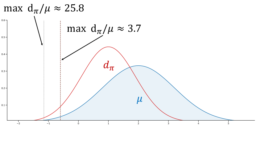
Note that decomposition of our error bound into on-support and off-support parts effectively achieves a bias-variance tradeoff. A small value of the concentrability threshold $C_{2}$ requires the choice of the distribution $\nu$ closer to $\mu$, which results in better estimation error guarantee (which is $\mathcal{O}(\sqrt{\nicefrac{{C_{2}}}{{n}}})$) when we transfer from $\mu$ to $\nu$, but potentially pays a high bias due to the mismatch between $d_{\pi}$ and $\nu$. A larger threshold permits more flexibility in choosing $\nu$ similar to $d_{\pi}$ for a smaller bias, but results in a larger variance and estimation error. Rather than commit to a particular tradeoff, our estimator automatically adapts to the best possible splitting (Figureย 1 illustrates this concept) by allowing us to choose the best threshold $C_{2}$. The on-support part matches the $n$ rate (fast rate error bound) of API or AVI analysis (e.g.,ย [Pires and Szepesvรกri, 2012; Lazaric etย al., 2012; Chen and Jiang, 2019]). The dependency on horizon is only linear and matches the best previous result with concentrability assumptionย [Xie and Jiang, 2020]. For the off-support part, it depends on the off-support mass $d_{\pi}\setminus\nu$ and the โ€œqualityโ€ of the off-support estimation: if all value functions in the version space are close to each other in the off-support region for policy $\pi$, the gap between $J(\pi)$ and $J({\widehat{\pi}})$ can still be small even with a large off-support mass. The following corollary formally states this property.

Corollary 1 (โ€œDouble Robustnessโ€).

Under conditions of Theoremย 3.1, for any $\pi$ and $C_{2}\geq 0$, $\mathrm{err}_{\mathrm{off}}(\pi)=0$ when either (1) $\mathscr{C}(d_{\pi};\mu,\mathcal{F},\pi)\leq C_{2}$, or, (2) $\Delta f_{\pi}-\gamma\mathcal{P}^{\pi}\Delta f_{\pi}\equiv 0$.

Adaptive guarantees by algorithm design.

As mentioned above, Theoremย 3.1 implicitly selects the best bias-variance decomposition through the best choice of $C_{2}$ in hindsight, with this decomposition being purely a proof technique, not an knob in the algorithm. In contrast, many prior approachesย [Liu etย al., 2020; Fujimoto etย al., 2019; Kumar etย al., 2019] employ explicit thresholds to control density ratios in their algorithms, which makes the tradeoff a hyperparameter in their algorithms. Since choosing hyperparameters is particularly challenging in offline RL, where even policy evaluation can be unreliable, this novel axis of adaptivity is an extremely desirable property of our approach.

Comparison to guarantees in the exploratory setting.

When a dataset with full coverage is given, classical analyses provide near-optimality guarantees that compete with the optimal policy $\pi^{\star}$ with a polynomial sample complexity, when ฯ€โ‹†โˆˆฮ superscript๐œ‹โ‹†ฮ \pi^{\star}\in\Pi and both realizability and completeness hold for $\mathcal{F}$; seeย [Antos etย al., 2008] for a representative analysis. As mentioned earlier, such analysis often requires boundedness of $\|\nu/\mu\|_{\infty}$ for all admissible distributions ฮฝโˆˆ{dฯ€:ฯ€โˆˆฮ }๐œˆconditional-setsubscript๐‘‘๐œ‹๐œ‹ฮ \nu\in\{d_{\pi}:\pi\in\Pi\}. On the other hand, it is easily seen that we can compete with $\pi^{\star}$ under much weaker conditions.

Corollary 2 (Competing with optimal policy).

Under conditions of Theoremย 3.1, if $\mathscr{C}(d_{\pi^{\star}};\mu,\mathcal{F},\pi^{\star})\leq C_{2}$, we have

Jโ€‹(ฯ€โ‹†)โˆ’Jโ€‹(ฯ€^)โ‰ค๐’ชโ€‹(Vmaxโ€‹C21โˆ’ฮณโ€‹logโก|โ„ฑ|โ€‹|ฮ |ฮดn+C2โ€‹(ฮตโ„ฑ,โ„ฑ+ฮตโ„ฑ)1โˆ’ฮณ).๐ฝsuperscript๐œ‹โ‹†๐ฝ^๐œ‹๐’ชsubscript๐‘‰subscript๐ถ21๐›พโ„ฑฮ ๐›ฟ๐‘›subscript๐ถ2subscript๐œ€โ„ฑโ„ฑsubscript๐œ€โ„ฑ1๐›พJ(\pi^{\star})-J({\widehat{\pi}})\leq~{}\mathcal{O}\left(\frac{V_{\max}\sqrt{C_{2}}}{1-\gamma}\sqrt{\frac{\log\frac{|\mathcal{F}||\Pi|}{\delta}}{n}}+\frac{\sqrt{C_{2}(\varepsilon_{\mathcal{F},\mathcal{F}}+\varepsilon_{\mathcal{F}})}}{1-\gamma}\right). (3.7)

Notably, these milder coverage assumptions in Corollariesย 1 andย 2 provide offline RL counterparts to the benefits of policy-gradient-style methods with online access to the environmentย [Kakade and Langford, 2002; Scherrer, 2014; Agarwal etย al., 2019].

Comparison withย Liu etย al. [2020].

The closest prior result to our work is that ofย [Liu etย al., 2020], who develop a pessimistic estimator that truncates Bellman backups from state-action pairs infrequently visited by $\mu$, and analyzes the resulting pessimistic policy and value iteration algorithms under general function approximation. For truncating Bellman backups, however, their work requires estimating the state-action distribution of data, which can be challenging in high-dimensions and they incur additional errors from density estimation which we avoid. Further, their algorithms only compete with policies $\pi$ where $\|d_{\pi}/\mu\|_{\infty}$ is bounded instead of the more general result that we provide, and makes their results vacuous in a linear MDP setting under typical feature coverage assumptions.

Safe Policy Improvement.

Some prior worksย [e.g. Laroche etย al., 2019; Liu etย al., 2020] discuss the scenario where the dataset $\mathcal{D}$ is collected with a behavior policy $\pi_{b}$ with $\mu=d_{\pi_{b}}$, and demonstrate that their algorithms always return a policy competitive with $\pi_{b}$. In our setup, this is straightforward as $d_{\pi_{b}}$ is always covered, as shown next.

Corollary 3 (Bounded degradation from behavior policy).

Under conditions of Theoremย 3.1, if $\mu=d_{\pi_{b}}$ for some policy ฯ€bโˆˆฮ subscript๐œ‹๐‘ฮ \pi_{b}\in\Pi, we have

Jโ€‹(ฯ€b)โˆ’Jโ€‹(ฯ€^)โ‰ค๐’ชโ€‹(Vmax1โˆ’ฮณโ€‹logโก|โ„ฑ|โ€‹|ฮ |ฮดn+ฮตโ„ฑ,โ„ฑ+ฮตโ„ฑ1โˆ’ฮณ).๐ฝsubscript๐œ‹๐‘๐ฝ^๐œ‹๐’ชsubscript๐‘‰1๐›พโ„ฑฮ ๐›ฟ๐‘›subscript๐œ€โ„ฑโ„ฑsubscript๐œ€โ„ฑ1๐›พ\displaystyle J(\pi_{b})-J({\widehat{\pi}})\leq\mathcal{O}\left(\frac{V_{\max}}{1-\gamma}\sqrt{\frac{\log\frac{|\mathcal{F}||\Pi|}{\delta}}{n}}+\frac{\sqrt{\varepsilon_{\mathcal{F},\mathcal{F}}+\varepsilon_{\mathcal{F}}}}{1-\gamma}\right). (3.8)
Proof sketch of Theoremย 3.1.

We now briefly describe the core ideas in the proof. More detailed arguments are deferred to the full proof in Appendixย B.1.

The key to prove Theoremย 3.1 is to translate the $J(\pi)-J({\widehat{\pi}})$ to the Bellman error of value functions in the version space $\mathcal{F}_{\pi,\varepsilon}$. Our main proving strategies are as follows:

  1. 1.

    As the selection of $\varepsilon=\varepsilon_{r}$ ensures the accurate estimation $Q^{\pi}$ is contained in the version space $\mathcal{F}_{{\widehat{\pi}},\varepsilon}$ for any $\pi$, we can obtain Jโ€‹(ฯ€)โˆ’Jโ€‹(ฯ€^)โ‰คmaxfโˆˆโ„ฑฯ€,ฮตโกfโ€‹(s0,ฯ€)โˆ’minfโˆˆโ„ฑฯ€^,ฮตโกfโ€‹(s0,ฯ€^)+approximation error๐ฝ๐œ‹๐ฝ^๐œ‹subscript๐‘“subscriptโ„ฑ๐œ‹๐œ€๐‘“subscript๐‘ 0๐œ‹subscript๐‘“subscriptโ„ฑ^๐œ‹๐œ€๐‘“subscript๐‘ 0^๐œ‹approximation errorJ(\pi)-J({\widehat{\pi}})\leq\max_{f\in\mathcal{F}_{\pi,\varepsilon}}f(s_{0},\pi)-\min_{f\in\mathcal{F}_{{\widehat{\pi}},\varepsilon}}f(s_{0},{\widehat{\pi}})+\text{approximation error}.

  2. 2.

    By the optimality of ${\widehat{\pi}}$, we have minfโˆˆโ„ฑฯ€^,ฮตโกfโ€‹(s0,ฯ€^)โ‰ฅminfโˆˆโ„ฑฯ€,ฮตโกfโ€‹(s0,ฯ€)subscript๐‘“subscriptโ„ฑ^๐œ‹๐œ€๐‘“subscript๐‘ 0^๐œ‹subscript๐‘“subscriptโ„ฑ๐œ‹๐œ€๐‘“subscript๐‘ 0๐œ‹\min_{f\in\mathcal{F}_{{\widehat{\pi}},\varepsilon}}f(s_{0},{\widehat{\pi}})\geq\min_{f\in\mathcal{F}_{\pi,\varepsilon}}f(s_{0},\pi). This indicates that Jโ€‹(ฯ€)โˆ’Jโ€‹(ฯ€^)โ‰คmaxfโˆˆโ„ฑฯ€,ฮตโกfโ€‹(s0,ฯ€)โˆ’minfโˆˆโ„ฑฯ€,ฮตโกfโ€‹(s0,ฯ€)+approximation error๐ฝ๐œ‹๐ฝ^๐œ‹subscript๐‘“subscriptโ„ฑ๐œ‹๐œ€๐‘“subscript๐‘ 0๐œ‹subscript๐‘“subscriptโ„ฑ๐œ‹๐œ€๐‘“subscript๐‘ 0๐œ‹approximation errorJ(\pi)-J({\widehat{\pi}})\leq\max_{f\in\mathcal{F}_{\pi,\varepsilon}}f(s_{0},\pi)-\min_{f\in\mathcal{F}_{\pi,\varepsilon}}f(s_{0},\pi)+\text{approximation error}.

  3. 3.

    By using a standard telescoping argument (e.g.,ย [Xie and Jiang, 2020, Lemma 1]), maxfโˆˆโ„ฑฯ€,ฮตโกfโ€‹(s0,ฯ€)โˆ’minfโˆˆโ„ฑฯ€,ฮตโกfโ€‹(s0,ฯ€)subscript๐‘“subscriptโ„ฑ๐œ‹๐œ€๐‘“subscript๐‘ 0๐œ‹subscript๐‘“subscriptโ„ฑ๐œ‹๐œ€๐‘“subscript๐‘ 0๐œ‹\max_{f\in\mathcal{F}_{\pi,\varepsilon}}f(s_{0},\pi)-\min_{f\in\mathcal{F}_{\pi,\varepsilon}}f(s_{0},\pi) can be upper bounded by the Bellman error of argmaxfโˆˆโ„ฑฯ€,ฮตfโ€‹(s0,ฯ€)subscriptargmax๐‘“subscriptโ„ฑ๐œ‹๐œ€๐‘“subscript๐‘ 0๐œ‹\mathop{\mathrm{argmax}}_{f\in\mathcal{F}_{\pi,\varepsilon}}f(s_{0},\pi) and argminfโˆˆโ„ฑฯ€,ฮตfโ€‹(s0,ฯ€)subscriptargmin๐‘“subscriptโ„ฑ๐œ‹๐œ€๐‘“subscript๐‘ 0๐œ‹\mathop{\mathrm{argmin}}_{f\in\mathcal{F}_{\pi,\varepsilon}}f(s_{0},\pi) over distribution $d_{\pi}$.

After combining all the three steps above together and considering the distribution shift effect, we complete the proof. โˆŽ

3.1 Results for Linear Function Approximation

Here we perform a case study in linear function approximation. We will show that our resultsโ€”when instantiated under linear function approximation (with realizability and completeness assumptions)โ€”automatically provides state-of-the-art guarantees, improving over existing results specialized to this setting by a factor of $\mathcal{O}(d)$ย [Jin etย al., 2021] when the action space is finite and small.

We recall the linear function approximation setup (we set $R_{\max}=1$ and $V_{\max}=\tfrac{1}{1-\gamma}$ for consistency with literature).333 In an earlier version of the paper we used the greedy policy class and made a mistake in the proof; correcting the proof would yield an additional $|\mathcal{A}|$ dependence in the bound. Here we fixed this issue by changing to the softmax policy class and leveraging covering arguments and concentration bounds from Zanette etย al. [2021] and Cheng etย al. [2022], respectively.

Definition 2 (Linear Function Approximation).

Let $\phi:\mathcal{S}\times\mathcal{A}\to\mathbb{R}^{d}$ be a feature mapping. Without loss of generality, we assume โ€–ฯ•โ€‹(s,a)โ€–2โ‰ค1subscriptnormitalic-ฯ•๐‘ ๐‘Ž21\|\phi(s,a)\|_{2}\leq 1, โˆ€(s,a)โˆˆ๐’ฎร—๐’œfor-all๐‘ ๐‘Ž๐’ฎ๐’œ\forall(s,a)\in\mathcal{S}\times\mathcal{A}. We define the value-function class $\mathcal{F}_{\Phi}$ as $\mathcal{F}_{\Phi}\coloneqq\{\phi(\cdot,\cdot)^{\mathsf{T}}\theta:\theta\in\mathbb{R}^{d},\|\theta\|_{2}\leq L_{1},\phi(\cdot,\cdot)^{\mathsf{T}}\theta\in[0,V_{\max}]\}$, and the policy class ฮ ฮฆsubscriptฮ ฮฆ\Pi_{\Phi} is the softmax policies of ฮ ฮฆโ‰”{ฯ•โ€‹(โ‹…,โ‹…)๐–ณโ€‹ฮธ:ฮธโˆˆโ„d,โ€–ฮธโ€–2โ‰คL2}โ‰”subscriptฮ ฮฆconditional-setitalic-ฯ•superscriptโ‹…โ‹…๐–ณ๐œƒformulae-sequence๐œƒsuperscriptโ„๐‘‘subscriptnorm๐œƒ2subscript๐ฟ2\Pi_{\Phi}\coloneqq\{\phi(\cdot,\cdot)^{\mathsf{T}}\theta:\theta\in\mathbb{R}^{d},\|\theta\|_{2}\leq L_{2}\}.

Assumption 3 (Realizability and Completeness).

$\varepsilon_{\mathcal{F},\mathcal{F}}=\varepsilon_{\mathcal{F}}=0$.

Note that, when the feature mapping $\phi(\cdot,\cdot)$ is the one induced by the linear MDP [Jin etย al., 2020], it automatically ensures that $\mathcal{F}_{\Phi}$ satisfies Assumptionsย 3. We also highlight that the standard linear function approximation or linear MDP setup does not entail all the assumptions needed byย Liu etย al. [2020] as mentioned earlier. To be consistent with the above results of general function classes, below we will present the results using the upper bound $V_{\max}$ on the functions in $\mathcal{F}_{\Phi}$, where $V_{\max}$ in such a bound can be replaced directly by using the value function radius $L_{1}$. In Appendixย B.2, we show that the policy class ฮ ฮฆsubscriptฮ ฮฆ\Pi_{\Phi} contains a near-optimal policy as long as $L_{2}$ is moderately large.

Below is our main result in the linear function approximation setting.

Theorem 3.2.

Suppose the value-function class $\mathcal{F}_{\Phi}$ is a linear function class that satisfies realizability and completeness (Definitionย 2 and Assumptionย 3) and ${\widehat{\pi}}$ is the output of Eq.(3.2) using value-function class $\mathcal{F}_{\Phi}$ and policy class ฮ ฮฆsubscriptฮ ฮฆ\Pi_{\Phi}. If we choose $\varepsilon=(cV_{\max}^{2}d\log\frac{nL_{1}L_{2}}{V_{\max}\delta})/{n}$, then, for any policy ฯ€โˆˆฮ ฮฆ๐œ‹subscriptฮ ฮฆ\pi\in\Pi_{\Phi}, we have

Jโ€‹(ฯ€)โˆ’Jโ€‹(ฯ€^)โ‰ค๐’ชโ€‹(Vmax1โˆ’ฮณโ€‹dโ€‹logโกnโ€‹L1โ€‹L2Vmaxโ€‹ฮดnโ€‹๐”ผdฯ€โ€‹[ฯ•โ€‹(s,a)๐–ณโ€‹ฮฃ๐’Ÿโˆ’1โ€‹ฯ•โ€‹(s,a)]),๐ฝ๐œ‹๐ฝ^๐œ‹๐’ชsubscript๐‘‰1๐›พ๐‘‘๐‘›subscript๐ฟ1subscript๐ฟ2subscript๐‘‰๐›ฟ๐‘›subscript๐”ผsubscript๐‘‘๐œ‹delimited-[]italic-ฯ•superscript๐‘ ๐‘Ž๐–ณsuperscriptsubscriptฮฃ๐’Ÿ1italic-ฯ•๐‘ ๐‘Ž\displaystyle J(\pi)-J({\widehat{\pi}})\leq\mathcal{O}\left(\frac{V_{\max}}{1-\gamma}\sqrt{\frac{d\log\frac{nL_{1}L_{2}}{V_{\max}\delta}}{n}}\mathbb{E}_{d_{\pi}}\left[\sqrt{\phi(s,a)^{\mathsf{T}}\Sigma_{\mathcal{D}}^{-1}\phi(s,a)}\right]\right), (3.9)

where $c$ is an absolute constant, and ฮฃ๐’Ÿโ‰”๐”ผ๐’Ÿโ€‹[ฯ•โ€‹(s,a)โ€‹ฯ•โ€‹(s,a)๐–ณ]โ‰”subscriptฮฃ๐’Ÿsubscript๐”ผ๐’Ÿdelimited-[]italic-ฯ•๐‘ ๐‘Žitalic-ฯ•superscript๐‘ ๐‘Ž๐–ณ\Sigma_{\mathcal{D}}\coloneqq\mathbb{E}_{\mathcal{D}}\left[\phi(s,a)\phi(s,a)^{\mathsf{T}}\right].

The detailed proof of Theoremย 3.2 is provided in Appendixย B.2. Our guarantee is structurally very similar to that ofย Jin etย al. [2021, Theorem 4.4], except that we only need linear function approximation with realizability and completeness assumptions, and they consider the finite-horizon linear MDP setting. If we translate their result to the discounted setting by setting $H=\mathcal{O}(1/(1-\gamma))$, we enjoy a net improvement of order $\mathcal{O}(d)$ in sample complexity when the action space is finite and small. To make it concrete, that is $\mathcal{O}(\sqrt{\nicefrac{{d^{2}\log(dn/\delta)}}{{n}}})$ vs.ย ๐’ชโ€‹(dโ€‹logโก(nโ€‹L1โ€‹L2/Vmaxโ€‹ฮด)/n)๐’ช๐‘‘๐‘›subscript๐ฟ1subscript๐ฟ2subscript๐‘‰๐›ฟ๐‘›\mathcal{O}(\sqrt{\nicefrac{{d\log(nL_{1}L_{2}/V_{\max}\delta)}}{{n}}}) error bounds. Careful readers may notice that Jin etย al. [2021] compete with $\pi^{\star}$ whereas we can only compete with the best policy in ฮ ฮฆsubscriptฮ ฮฆ\Pi_{\Phi}, but this can be easily addressed without changing the order of our error bound: in Appendixย B.2 we show that selecting a large policy radius (e.g., $L_{2}=\nicefrac{{L_{1}\log|\mathcal{A}|\sqrt{n}}}{{V_{\max}}}$) ensures the existence of a good policy in ฮ ฮฆsubscriptฮ ฮฆ\Pi_{\Phi}, denoted as $\pi_{\Phi}^{\star}$, whose suboptimality is no larger than the bound in Theoremย 3.2, and hence we can compete with $\pi^{\star}$ and the additive error will be absorbed by the big-Oh.444This introduces another subtle difference between our bound and Jin etย al. [2021] when both compete with $\pi^{\star}$: Jin etย al. [2021] requires coverage of $\pi^{\star}$, whereas we require coverage of $\pi_{\Phi}^{\star}$. Our bound also shows that having a full-rank $\Sigma_{\mathcal{D}}$ (which is ensured by a full-rank covariance under $\mu$) is sufficient for consistent offline RL in linear function approximation. Crucially, the full-rank covariance is an easily checkable condition on data, as opposed to unverifiable concentrability assumptions. As a caveat, our results do not imply a computationally efficient algorithm, as a naรฏve implementation involves evaluating each policy pessimistically to pick the best. We discuss a computationally efficient adaptation of our approach in the next section.

4 Practical Algorithm โ€” Regularized Offline Policy Optimization

A major challenge using the proposed algorithm in Sectionย 3 in practice is that searching the policy with the best pessimistic evaluation over the policy space ฮ ฮ \Pi is not computationally tractable. In this section, we present a practical algorithm that is computationally efficient assuming access to a (regularized) loss minimization oracle over the value function class $\mathcal{F}$, and also comes with rigorous theoretical guarantees.

Algorithm 1 PSPI: Pessimistic Soft Policy Iteration

Input: Batch data $\mathcal{D}$, regularization coefficient $\lambda$.

1:Initialize policy $\pi_{1}$ as the uniform policy.
2:forย t=1,2,โ€ฆ,T๐‘ก12โ€ฆ๐‘‡t=1,2,\dotsc,Tย do
3:ย ย ย ย ย Obtain the pessimistic estimation for $\pi_{t}$ as $f_{t}$,
ftโ†argminfโˆˆโ„ฑ(fโ€‹(s0,ฯ€t)+ฮปโ€‹โ„ฐโ€‹(f,ฯ€t;๐’Ÿ)),โ†subscript๐‘“๐‘กsubscriptargmin๐‘“โ„ฑ๐‘“subscript๐‘ 0subscript๐œ‹๐‘ก๐œ†โ„ฐ๐‘“subscript๐œ‹๐‘ก๐’Ÿ\displaystyle f_{t}\leftarrow\mathop{\mathrm{argmin}}_{f\in\mathcal{F}}\left(f(s_{0},\pi_{t})+\lambda\mathcal{E}(f,\pi_{t};\mathcal{D})\right), (4.1)
where $\mathcal{E}(f,\pi_{t};\mathcal{D})$ is defined in Eq.(3.1).
4:ย ย ย ย ย Calculate $\pi_{t+1}$ by,
ฯ€t+1โ€‹(a|s)โˆฯ€tโ€‹(a|s)โ€‹expโก(ฮทโ€‹ftโ€‹(s,a)),โˆ€s,aโˆˆ๐’ฎร—๐’œ.formulae-sequenceproportional-tosubscript๐œ‹๐‘ก1conditional๐‘Ž๐‘ subscript๐œ‹๐‘กconditional๐‘Ž๐‘ ๐œ‚subscript๐‘“๐‘ก๐‘ ๐‘Žfor-all๐‘ ๐‘Ž๐’ฎ๐’œ\displaystyle\pi_{t+1}(a|s)\propto\pi_{t}(a|s)\exp\left(\eta f_{t}(s,a)\right),~{}\forall s,a\in\mathcal{S}\times\mathcal{A}. (4.2)
5:endย for
6:Output ${\bar{\pi}}\coloneqq\mathsf{Unif}(\pi_{[1:T]})$. $\triangleright$ uniformly mix $\pi_{1},\ldots,\pi_{T}$ at the trajectory level

Our practical algorithm is summarized in Algorithmย 1. It has three key differences from the information-theoretic version in Eq.(3.2):

  1. 1.

    The pessimistic policy evaluation is now performed via regularization (Lineย 3) instead of constrained optimization.

  2. 2.

    Instead of searching over an explicit policy space ฮ ฮ \Pi, we search over a policy class implicitly induced from $\mathcal{F}$ (defined in Eq.(4.3)) and therefore no longer have a policy class independent of $\mathcal{F}$ separately, which is a common practice in API-style algorithmsย [Munos, 2003; Antos etย al., 2008; Lazaric etย al., 2012].

  3. 3.

    We optimize the policy using mirror descent updates, which yields computationally tractable optimization over the implicit policy class. This property has been leveraged in many prior works, although typically in online RL settingsย [Even-Dar etย al., 2009; Agarwal etย al., 2019; Geist etย al., 2019; Cai etย al., 2020; Shani etย al., 2020].

Note that the use of a specific policy class above can be relaxed if a stronger structural assumption is made on the MDP (e.g., linear MDPsย [Jin etย al., 2020, 2021]).

4.1 Analysis of Algorithmย 1

We now provide the analysis of Algorithmย 1 in this section. For ease of presentation, we formally define the implicit policy class for this section:

ฮ SPI:={ฯ€โ€ฒ(โ‹…|s)โˆexp(ฮทโˆ‘i=1tf(t)(s,โ‹…)):1โ‰คtโ‰คT,f(1),โ€ฆ,f(i)โˆˆโ„ฑ},\Pi_{\textrm{SPI}}:=\{\pi^{\prime}(\cdot|s)\propto\exp(\eta\sum_{i=1}^{t}f^{(t)}(s,\cdot)):1\leq t\leq T,f^{(1)},\ldots,f^{(i)}\in\mathcal{F}\}, (4.3)

which is the natural policy class for soft policy-iteration approaches. The following theorem describes the performance guarantee of ${\bar{\pi}}$.

Theorem 4.1.

Let $\lambda=\sqrt[3]{\nicefrac{{V_{\max}}}{{(1-\gamma)^{2}\varepsilon_{r}^{2}}}}$ with $\varepsilon_{r}$ in Eq.(3.4), $\eta=\sqrt{\frac{\log|\mathcal{A}|}{2V_{\max}^{2}T}}$, and ${\bar{\pi}}$ be obtained from Algorithmย 1. For any policy $\pi:\mathcal{S}\to\Delta(\mathcal{A})$ we wish to compete with, suppose Assumptionsย 1 andย 2 hold with respect to the policy class ฮ SPIโˆช{ฯ€}subscriptฮ SPI๐œ‹\Pi_{\textrm{SPI}}\cup\{\pi\}. Then, for any constant $C_{2}\geq 1$, we have with probability at least $1-\delta$,

$\displaystyle~{}J(\pi)-J({\bar{\pi}})$ (4.4)
$\displaystyle\leq$ $\displaystyle~{}\underbrace{\mathcal{O}\left(\sqrt{C_{2}}\left(\frac{\sqrt{\varepsilon_{\mathcal{F},\mathcal{F}}+\varepsilon_{\mathcal{F}}}}{1-\gamma}+\frac{V_{\max}}{1-\gamma}\sqrt[3]{\frac{T\log\frac{|\mathcal{F}|}{\delta}}{n}}+\sqrt[3]{\frac{V_{\max}\varepsilon_{\mathcal{F}}}{(1-\gamma)^{2}}}\right)\right)}_{\text{$\mathrm{err}_{\mathrm{on}}(\pi)$: on-support error}}+\underbrace{\mathcal{O}\left(\frac{V_{\max}}{1-\gamma}\sqrt{\frac{\log|\mathcal{A}|}{T}}\right)}_{\text{optimization error}}$ (4.5)
+1Tโ€‹โˆ‘t=1T(minฮฝ:๐’žโ€‹(ฮฝ;ฮผ,โ„ฑ,ฯ€t)โ‰คC2โก|โˆ‘(s,a)โˆˆ๐’ฎร—๐’œ(dฯ€โˆ–ฮฝ)โ€‹(s,a)โ€‹[ftโ€‹(s,a)โˆ’(๐’ฏฯ€tโ€‹ft)โ€‹(s,a)]1โˆ’ฮณ|)โŸerroffโ€‹(ฯ€): off-support error,subscriptโŸ1๐‘‡superscriptsubscript๐‘ก1๐‘‡subscript:๐œˆ๐’ž๐œˆ๐œ‡โ„ฑsubscript๐œ‹๐‘กsubscript๐ถ2subscript๐‘ ๐‘Ž๐’ฎ๐’œsubscript๐‘‘๐œ‹๐œˆ๐‘ ๐‘Ždelimited-[]subscript๐‘“๐‘ก๐‘ ๐‘Žsuperscript๐’ฏsubscript๐œ‹๐‘กsubscript๐‘“๐‘ก๐‘ ๐‘Ž1๐›พerroff(ฯ€): off-support error\displaystyle~{}+\underbrace{\frac{1}{T}\sum_{t=1}^{T}\left(\min_{\nu:\mathscr{C}(\nu;\mu,\mathcal{F},\pi_{t})\leq C_{2}}\left|\sum_{(s,a)\in\mathcal{S}\times\mathcal{A}}\frac{(d_{\pi}\setminus\nu)(s,a)\left[f_{t}(s,a)-(\mathcal{T}^{\pi_{t}}f_{t})(s,a)\right]}{1-\gamma}\right|\right)}_{\text{$\mathrm{err}_{\mathrm{off}}(\pi)$: off-support error}}, (4.6)

where $\mathscr{C}(\nu;\mu,\mathcal{F},\pi_{t})$ is defined in Definitionย 1, (dฯ€โˆ–ฮฝ)โ€‹(s,a)โ‰”maxโก(dฯ€โ€‹(s,a)โˆ’ฮฝโ€‹(s,a),0)โ‰”subscript๐‘‘๐œ‹๐œˆ๐‘ ๐‘Žsubscript๐‘‘๐œ‹๐‘ ๐‘Ž๐œˆ๐‘ ๐‘Ž0(d_{\pi}\setminus\nu)(s,a)\coloneqq\max(d_{\pi}(s,a)-\nu(s,a),0).

We provide a proof sketch of Theoremย 4.1 at the end of this section, and defer the full proof to Appendixย C. We now make a few remarks about the results in Theoremย 4.1.

Measurement of distribution shift effect.

Compared with the information-theoretical result (provided in Theoremย 3.1), the measurement of distribution shift in Theoremย 4.1 depends on the optimization trajectory. That is, it measures the distance between two distribution $\nu$ and $\mu$ by $\mathscr{C}(\nu;\mu,\mathcal{F},\pi_{t})$ ($\pi_{[1:T]}$ is the sequence of policies produced by the algorithm) whereas Theoremย 3.1 uses $\mathscr{C}(\nu;\mu,\mathcal{F},\pi)$ ($\pi$ is the baseline policy we compete with). We remark that both of these two measurements are weaker then traditional density-ratio definitions (e.g.,ย [Munos and Szepesvรกri, 2008; Chen and Jiang, 2019; Xie and Jiang, 2020]) as we demonstrated before, as the dependence of $\mathscr{C}$ on $\pi$ is relatively secondary.

Dependence on $T$.

The number of optimization rounds $T$ affects the bound in two opposite ways: as $T$ increases, the optimization error term decreases, whereas the second term of the on-support error increases. The latter increase is due to the complexity of the implicit policy class ฮ ฮ \Pi growing exponentially with $T$, which affects our concentration bounds. To optimize the bound, the optimal choice is $T=\mathcal{O}(n^{2/5})$, leading to an overall $\mathcal{O}(n^{-1/5})$ rate. While such a rate is relatively slow, we remark that the complexity bound of ฮ ฮ \Pi is conservative, and in certain cases it is possible to obtain much sharper bounds: for example, in linear function approximation (Sectionย 3.1), ฮ SPIsubscriptฮ SPI\Pi_{\textrm{SPI}} are a priori captured by the space of softmax policies, whose complexity has no dependence on $T$ (up to mild logarithmic dependence due to norms). That is, the $\mathrm{err}_{\mathrm{on}}(\pi)$ term in Theorem 4.1 reduces to $\widetilde{\mathcal{O}}(\frac{V_{\max}}{1-\gamma}\sqrt[3]{{d}/{n}})$ ($\varepsilon_{\mathcal{F},\mathcal{F}}=\varepsilon_{\mathcal{F}}=0$ in linear function approximation), and yields an overall $\mathcal{O}(n^{-1/3})$ rate.

Bias-variance decomposition.

Similar to Theoremย 3.1, Theoremย 4.1 also allows arbitrary decomposition of the error bound into on-support and off-support components by setting the concentrability threshold $C_{2}$, which serves as a bias-variance tradeoff as before. In fact, the splitting can be done separately for each $\pi_{t}$ in $1\leq t\leq T$ and we omit such flexibility for readability. The optimization error does not depend on the splitting. Our performance guarantee naturally adapts to the best possible decomposition as before. As in Theoremย 3.1, if the estimation on the off-support region is โ€œhigh-qualityโ€, we can further simplify the performance guarantees, but the requirement of โ€œhigh-qualityโ€ is different from that of Corollaryย 1. We make it formal in the following corollary.

Corollary 4 (โ€œDouble Robustnessโ€).

For any $\pi$ and $C_{2}\geq 0$, $\mathrm{err}_{\mathrm{off}}(\pi)=0$ when either (1) $\mathscr{C}(d_{\pi};\mu,\mathcal{F},\pi_{t})\leq C_{2}$ for all $t\in[T]$, or, (2) $f_{t}-\mathcal{T}^{\pi_{t}}\Delta f_{t}\equiv 0$ for all $t\in[T]$.

We note that the conditions above depend on the optimization trajectory through their dependence on $\pi_{t}$, but can be made algorithm-independent by instead asserting the stronger requirement that $\mathscr{C}(d_{\pi},\mu,\mathcal{F},\pi^{\prime})\leq C_{2}$ for all ฯ€โ€ฒโˆˆฮ SPIsuperscript๐œ‹โ€ฒsubscriptฮ SPI\pi^{\prime}\in\Pi_{\textrm{SPI}} in the first condition.

Competing with the optimal policy.

As before, we can provide a guarantee for competing with the optimal policy, under coverage assumptions weaker than the typical batch RL literature, albeit slightly stronger than those of Corollaryย 2. We state the formal result below.

Corollary 5 (Competing with optimal policy).

Under conditions of Theoremย 4.1, if $\mathscr{C}(d_{\pi^{\star}};\mu,\mathcal{F},\pi)\leq C_{2}$ for all ฯ€โˆˆฮ SPI๐œ‹subscriptฮ SPI\pi\in\Pi_{\textrm{SPI}}, we have

$$J(\pi^{\star})-J({\widehat{\pi}})\leq~{}\mathcal{O}\left(\frac{V_{\max}\sqrt{C_{2}}}{1-\gamma}\left(\frac{\log\frac{|\mathcal{F}|}{\delta}\log|\mathcal{A}|}{n}\right)^{1/5}+\frac{\sqrt{C_{2}(\varepsilon_{\mathcal{F},\mathcal{F}}+\varepsilon_{\mathcal{F}})}}{1-\gamma}\right).$$ (4.7)

Note that the conditions of Corollaryย 5 are satisfied as before whenever $\|d_{\pi^{\star}}/\mu\|_{\infty}\leq C_{2}$.

Computationally-efficient implementation with linear function approximation

We remark that our algorithm is computationally efficient when the value-function class $\mathcal{F}$ is linear, that is, $\mathcal{F}\coloneqq\{\phi(\cdot,\cdot)^{\mathsf{T}}\theta:\theta\in\mathbb{R}^{d}\}$. In this case, the objective of Eq.(4.1) has a closed-form expression which is quadratic in $\theta$. In addition, under additional matrix invertibility conditions, Eq.(4.1) has a closed-form solution which generalizes LSTDQย [Lagoudakis and Parr, 2003; Sutton etย al., 2009; Dann etย al., 2014]. A similar connection has been made by Antos etย al. [2008], but our derivation is more general. See Appendix Appendixย D for further details.

We conclude the section with a proof sketch showing the key insights used in establishing the proof.

Proof sketch of Theoremย 4.1.

Our proof constructs a corresponding MDP $\mathcal{M}_{t}$ for every $f_{t},\pi_{t}$ pair. Each $\mathcal{M}_{t}$ has the same dynamics as the ground-truth MDP, but chooses a different reward function, such that $f_{t}$ is the $Q$-function of $\pi_{t}$ in $\mathcal{M}_{t}$, $Q^{\pi_{t}}_{\mathcal{M}_{t}}$ (we use the subscript of $\mathcal{M}_{t}$ to denote the corresponding value or operator in MDP $\mathcal{M}_{t}$). Our proof relies on some key properties of $\mathcal{M}_{t}$, such as $Q^{\pi}-\mathcal{T}^{\pi}_{\mathcal{M}_{t}}Q^{\pi}=f_{t}-\mathcal{T}^{\pi_{t}}f_{t}$. We decompose $J(\pi)-J(\bar{\pi})$ as follows.

$\displaystyle J(\pi)-J(\bar{\pi})\leq$ $\displaystyle~{}\underbrace{\frac{1}{T}\sum_{t=1}^{T}\left(J_{\mathcal{M}_{t}}(\pi)-J_{\mathcal{M}_{t}}(\pi_{t})\right)}_{\text{optimization error}}+\underbrace{\frac{1}{T}\sum_{t=1}^{T}\left(J(\pi)-J_{\mathcal{M}_{t}}(\pi)\right)}_{\text{controlled by }\|Q^{\pi}-\mathcal{T}^{\pi}_{\mathcal{M}_{t}}Q^{\pi}\|_{2,d_{\pi}}=\|f_{t}-\mathcal{T}^{\pi_{t}}f_{t}\|_{2,d_{\pi}}}$ (4.8)
$\displaystyle~{}+\text{approximation/statistical errors}.$ (4.9)

The proof is completed by bounding $\|f_{t}-\mathcal{T}^{\pi_{t}}f_{t}\|_{2,d_{\pi}}$ on both on-support and off-support regions. โˆŽ

5 Conclusions

This paper investigates sample-efficient offline reinforcement learning without data coverage assumptions (e.g., concentrability). To achieve that goal, our paper contributes several crucial improvements to the literature. We introduce the concept of Bellman-consistent pessimism. It enables the sample-efficient guarantees with only the Bellman-completeness assumption which is standard in the exploratory setting, whereas the point-wise/bonus-based pessimism popularly adopted in the literature usually requires stronger and/or extra assumptions. Algorithmically, we demonstrate how to implicitly infer a policy value lower bound through a version space and provide a tractable implementation. A particularly important aspect of our results is the ability to adapt to the best bias-variance tradeoff in the hindsight, which no prior algorithms achieve to the best of our knowledge. When applying our results in linear function approximation, we attain an $\mathcal{O}(d)$ improvement in sample complexity, compared with the best-known recent work of offline RL in linear MDPs, whenever the action space is finite and small.

As of limitations and future work, the sample complexity of our practical algorithm is worse than that of the information-theoretic approach, and it will be interesting to close this gap. Another future direction is to empirically evaluate PSPI on benchmarks and compare it to existing approaches.

Acknowledgment

Part of this work was carried out while TX and AA worked at Microsoft Research. NJ acknowledges funding support from the ARL Cooperative Agreement W911NF-17-2-0196, NSF IIS-2112471, and Adobe Data Science Research Award. The authors also thank Jinglin Chen for pointing out a mistake in the conference version of the paper (see Footnoteย 3).

References

  • Agarwal etย al. [2019] Alekh Agarwal, Shamย M Kakade, Jasonย D Lee, and Gaurav Mahajan. On the theory of policy gradient methods: Optimality, approximation, and distribution shift. arXiv preprint arXiv:1908.00261, 2019.
  • Antos etย al. [2008] Andrรกs Antos, Csaba Szepesvรกri, and Rรฉmi Munos. Learning near-optimal policies with bellman-residual minimization based fitted policy iteration and a single sample path. Machine Learning, 71(1):89โ€“129, 2008.
  • Bertsekas and Tsitsiklis [1996] Dimitriย P. Bertsekas and Johnย N. Tsitsiklis. Neuro-Dynamic Programming. Athena Scientific, 1st edition, 1996. ISBN 1886529108.
  • Cai etย al. [2020] Qiย Cai, Zhuoran Yang, Chi Jin, and Zhaoran Wang. Provably efficient exploration in policy optimization. In International Conference on Machine Learning, pages 1283โ€“1294. PMLR, 2020.
  • Chen and Jiang [2019] Jinglin Chen and Nan Jiang. Information-theoretic considerations in batch reinforcement learning. In International Conference on Machine Learning, pages 1042โ€“1051, 2019.
  • Cheng etย al. [2022] Ching-An Cheng, Tengyang Xie, Nan Jiang, and Alekh Agarwal. Adversarially trained actor critic for offline reinforcement learning. arXiv preprint arXiv:2202.02446, 2022.
  • Dann etย al. [2014] Christoph Dann, Gerhard Neumann, Jan Peters, etย al. Policy evaluation with temporal differences: A survey and comparison. Journal of Machine Learning Research, 15:809โ€“883, 2014.
  • Duan etย al. [2020] Yaqi Duan, Zeyu Jia, and Mengdi Wang. Minimax-optimal off-policy evaluation with linear function approximation. In International Conference on Machine Learning, pages 2701โ€“2709. PMLR, 2020.
  • Even-Dar etย al. [2009] Eyal Even-Dar, Shamย M Kakade, and Yishay Mansour. Online markov decision processes. Mathematics of Operations Research, 34(3):726โ€“736, 2009.
  • Farahmand etย al. [2010] Amirย Massoud Farahmand, Rรฉmi Munos, and Csaba Szepesvรกri. Error propagation for approximate policy and value iteration. In Advances in Neural Information Processing Systems, 2010.
  • Fujimoto etย al. [2019] Scott Fujimoto, David Meger, and Doina Precup. Off-policy deep reinforcement learning without exploration. In International Conference on Machine Learning, pages 2052โ€“2062, 2019.
  • Geist etย al. [2019] Matthieu Geist, Bruno Scherrer, and Olivier Pietquin. A theory of regularized markov decision processes. In International Conference on Machine Learning, pages 2160โ€“2169. PMLR, 2019.
  • Jiang etย al. [2017] Nan Jiang, Akshay Krishnamurthy, Alekh Agarwal, John Langford, and Robertย E Schapire. Contextual decision processes with low bellman rank are pac-learnable. In International Conference on Machine Learning, pages 1704โ€“1713. PMLR, 2017.
  • Jin etย al. [2020] Chi Jin, Zhuoran Yang, Zhaoran Wang, and Michaelย I Jordan. Provably efficient reinforcement learning with linear function approximation. In Conference on Learning Theory, pages 2137โ€“2143. PMLR, 2020.
  • Jin etย al. [2021] Ying Jin, Zhuoran Yang, and Zhaoran Wang. Is pessimism provably efficient for offline rl? In International Conference on Machine Learning, pages 5084โ€“5096. PMLR, 2021.
  • Kakade and Langford [2002] Sham Kakade and John Langford. Approximately optimal approximate reinforcement learning. In ICML, volumeย 2, pages 267โ€“274, 2002.
  • Kidambi etย al. [2020] Rahul Kidambi, Aravind Rajeswaran, Praneeth Netrapalli, and Thorsten Joachims. Morel: Model-based offline reinforcement learning. In Advances in Neural Information Processing Systems, 2020.
  • Konda and Tsitsiklis [2000] Vijayย R Konda and Johnย N Tsitsiklis. Actor-critic algorithms. In Advances in neural information processing systems, pages 1008โ€“1014. Citeseer, 2000.
  • Kumar etย al. [2019] Aviral Kumar, Justin Fu, Matthew Soh, George Tucker, and Sergey Levine. Stabilizing off-policy q-learning via bootstrapping error reduction. Advances in Neural Information Processing Systems, 32:11784โ€“11794, 2019.
  • Kumar etย al. [2020] Aviral Kumar, Aurick Zhou, George Tucker, and Sergey Levine. Conservative q-learning for offline reinforcement learning. Advances in Neural Information Processing Systems, 33:1179โ€“1191, 2020.
  • Lagoudakis and Parr [2003] Michailย G Lagoudakis and Ronald Parr. Least-squares policy iteration. The Journal of Machine Learning Research, 4:1107โ€“1149, 2003.
  • Laroche etย al. [2019] Romain Laroche, Paul Trichelair, and Remiย Tachet Desย Combes. Safe policy improvement with baseline bootstrapping. In International Conference on Machine Learning, pages 3652โ€“3661, 2019.
  • Lazaric etย al. [2012] Alessandro Lazaric, Mohammad Ghavamzadeh, and Rรฉmi Munos. Finite-sample analysis of least-squares policy iteration. Journal of Machine Learning Research, 13:3041โ€“3074, 2012.
  • Levine etย al. [2020] Sergey Levine, Aviral Kumar, George Tucker, and Justin Fu. Offline reinforcement learning: Tutorial, review, and perspectives on open problems. arXiv preprint arXiv:2005.01643, 2020.
  • Liu etย al. [2020] Yao Liu, Adith Swaminathan, Alekh Agarwal, and Emma Brunskill. Provably good batch off-policy reinforcement learning without great exploration. In Advances in Neural Information Processing Systems, 2020.
  • Munos [2003] Rรฉmi Munos. Error bounds for approximate policy iteration. In Proceedings of the Twentieth International Conference on International Conference on Machine Learning, pages 560โ€“567, 2003.
  • Munos and Szepesvรกri [2008] Rรฉmi Munos and Csaba Szepesvรกri. Finite-time bounds for fitted value iteration. Journal of Machine Learning Research, 9(5), 2008.
  • Pires and Szepesvรกri [2012] Bernardoย รvila Pires and Csaba Szepesvรกri. Statistical linear estimation with penalized estimators: an application to reinforcement learning. In Proceedings of the 29th International Coference on International Conference on Machine Learning, pages 1755โ€“1762, 2012.
  • Precup etย al. [2000] Doina Precup, Richardย S Sutton, and Satinderย P Singh. Eligibility traces for off-policy policy evaluation. In Proceedings of the Seventeenth International Conference on Machine Learning, pages 759โ€“766, 2000.
  • Scherrer [2014] Bruno Scherrer. Approximate policy iteration schemes: a comparison. In International Conference on Machine Learning, pages 1314โ€“1322. PMLR, 2014.
  • Shani etย al. [2020] Lior Shani, Yonathan Efroni, Aviv Rosenberg, and Shie Mannor. Optimistic policy optimization with bandit feedback. In International Conference on Machine Learning, pages 8604โ€“8613. PMLR, 2020.
  • Sutton etย al. [2009] Richardย S Sutton, Hamidย Reza Maei, Doina Precup, Shalabh Bhatnagar, David Silver, Csaba Szepesvรกri, and Eric Wiewiora. Fast gradient-descent methods for temporal-difference learning with linear function approximation. In Proceedings of the 26th Annual International Conference on Machine Learning, pages 993โ€“1000, 2009.
  • Szepesvรกri and Munos [2005] Csaba Szepesvรกri and Rรฉmi Munos. Finite time bounds for sampling based fitted value iteration. In Proceedings of the 22nd international conference on Machine learning, pages 880โ€“887, 2005.
  • Wang etย al. [2020] Ruosong Wang, Dean Foster, and Shamย M Kakade. What are the statistical limits of offline rl with linear function approximation? In International Conference on Learning Representations, 2020.
  • Wang etย al. [2021] Ruosong Wang, Yifan Wu, Ruslan Salakhutdinov, and Sham Kakade. Instabilities of offline rl with pre-trained neural representation. In International Conference on Machine Learning, pages 10948โ€“10960. PMLR, 2021.
  • Weisz etย al. [2021] Gellรฉrt Weisz, Philip Amortila, and Csaba Szepesvรกri. Exponential lower bounds for planning in mdps with linearly-realizable optimal action-value functions. In Algorithmic Learning Theory, pages 1237โ€“1264. PMLR, 2021.
  • Xie and Jiang [2020] Tengyang Xie and Nan Jiang. Q* approximation schemes for batch reinforcement learning: A theoretical comparison. In Conference on Uncertainty in Artificial Intelligence, pages 550โ€“559. PMLR, 2020.
  • Xie and Jiang [2021] Tengyang Xie and Nan Jiang. Batch value-function approximation with only realizability. In International Conference on Machine Learning, pages 11404โ€“11413. PMLR, 2021.
  • Yu etย al. [2020] Tianhe Yu, Garrett Thomas, Lantao Yu, Stefano Ermon, Jamesย Y Zou, Sergey Levine, Chelsea Finn, and Tengyu Ma. Mopo: Model-based offline policy optimization. Advances in Neural Information Processing Systems, 33:14129โ€“14142, 2020.
  • Zanette [2021] Andrea Zanette. Exponential lower bounds for batch reinforcement learning: Batch rl can be exponentially harder than online rl. In International Conference on Machine Learning, pages 12287โ€“12297. PMLR, 2021.
  • Zanette etย al. [2021] Andrea Zanette, Martinย J Wainwright, and Emma Brunskill. Provable benefits of actor-critic methods for offline reinforcement learning. Advances in neural information processing systems, 34, 2021.

Appendix

Appendix A Estimating Mean-Squared Bellman Error

We provide theoretical properties of $\mathcal{E}(f,\pi;\mathcal{D})$ (defined in Eq.(3.1)), when using it to bound Bellman error. Over this section, we use $\mu\times(\mathcal{P},R)$ to denote the joint distribution of (s,a,r,sโ€ฒ)๐‘ ๐‘Ž๐‘Ÿsuperscript๐‘ โ€ฒ(s,a,r,s^{\prime}).

All of our results in the appendix strongly depends one following two constants

  1. 1.

    $\varepsilon_{r}$ โ€” For any ฯ€โˆˆฮ ๐œ‹ฮ \pi\in\Pi, if $f_{\pi}$ is the โ€œbest estimationโ€ of $Q^{\pi}$ in $\mathcal{F}$ (formal definition of $f_{\pi}$: Eq.(A.1) for general function approximation, $Q^{\pi}$ for Linear function approximation), then $\mathcal{E}(f_{\pi},\pi;\mathcal{D})\leq\varepsilon_{r}$.

  2. 2.

    $\varepsilon_{b}$ โ€” For any function $f\in\mathcal{F}$ and any ฯ€โˆˆฮ ๐œ‹ฮ \pi\in\Pi, if $\mathcal{E}(f,\pi;\mathcal{D})\leq\varepsilon_{r}$, then $\|f-\mathcal{T}^{\pi}f\|_{2,\mu}^{2}\leq\varepsilon_{b}$.

The detailed discussion about $\varepsilon_{r}$ and $\varepsilon_{b}$ is provided in Appendix A.1 (general function approximation) and and Appendix A.2 (linear Linear function approximation).

A.1 Results for General Function Approximation

This section summarizes the results regarding $\mathcal{E}(f,\pi;\mathcal{D})$, we defer the full proof of Theoremย A.1 and Theoremย A.2 to Appendixย A.1.2.

Theorem A.1.

For any ฯ€โˆˆฮ ๐œ‹ฮ \pi\in\Pi, let $f_{\pi}$ be defined as follows,

$\displaystyle f_{\pi}\coloneqq$ $\displaystyle~{}\mathop{\mathrm{argmin}}_{f\in\mathcal{F}}\sup_{\text{admissible }\nu}\left\|f-\mathcal{T}^{\pi}f\right\|_{2,\nu}^{2}.$ (A.1)

Then, for $\mathcal{E}(f_{\pi},\pi;\mathcal{D})$ (defined in Eq.(3.1)), we have

โ„ฐโ€‹(fฯ€,ฯ€;๐’Ÿ)โ‰ค139โ€‹Vmax2โ€‹logโก|โ„ฑ|โ€‹|ฮ |ฮดn+39โ€‹ฮตโ„ฑโ‰•ฮตr.โ„ฐsubscript๐‘“๐œ‹๐œ‹๐’Ÿ139superscriptsubscript๐‘‰2โ„ฑฮ ๐›ฟ๐‘›39subscript๐œ€โ„ฑโ‰•subscript๐œ€๐‘Ÿ\displaystyle\mathcal{E}(f_{\pi},\pi;\mathcal{D})\leq\frac{139V_{\max}^{2}\log\frac{|\mathcal{F}||\Pi|}{\delta}}{n}+39\varepsilon_{\mathcal{F}}\eqqcolon\varepsilon_{r}. (A.2)

We now show that $\mathcal{E}(f,\pi;\mathcal{D})$ could effectively estimate $\|f-\mathcal{T}^{\pi}f\|_{2,\mu}^{2}$.

Theorem A.2.

For any ฯ€โˆˆฮ ๐œ‹ฮ \pi\in\Pi, $f\in\mathcal{F}$, and any $\varepsilon>0$, if $\mathcal{E}(f,\pi;\mathcal{D})\leq\varepsilon$, then,

โ€–fโˆ’๐’ฏฯ€โ€‹fโ€–2,ฮผโ‰คVmaxโ€‹231โ€‹logโก|โ„ฑ|โ€‹|ฮ |ฮดn+ฮตโ„ฑ,โ„ฑ+ฮตโ„ฑ,โ„ฑ+ฮต.subscriptnorm๐‘“superscript๐’ฏ๐œ‹๐‘“2๐œ‡subscript๐‘‰231โ„ฑฮ ๐›ฟ๐‘›subscript๐œ€โ„ฑโ„ฑsubscript๐œ€โ„ฑโ„ฑ๐œ€\displaystyle\|f-\mathcal{T}^{\pi}f\|_{2,\mu}\leq V_{\max}\sqrt{\frac{231\log\frac{|\mathcal{F}||\Pi|}{\delta}}{n}}+\sqrt{\varepsilon_{\mathcal{F},\mathcal{F}}}+\sqrt{\varepsilon_{\mathcal{F},\mathcal{F}}+\varepsilon}. (A.3)

We also define $\sqrt{\varepsilon_{b}}$ when setting $\varepsilon=\varepsilon_{r}$ in Eq.(A.3), i.e.,

ฮตbโ‰”Vmaxโ€‹231โ€‹logโก|โ„ฑ|โ€‹|ฮ |ฮดn+ฮตโ„ฑ,โ„ฑ+ฮตโ„ฑ,โ„ฑ+ฮตr.โ‰”subscript๐œ€๐‘subscript๐‘‰231โ„ฑฮ ๐›ฟ๐‘›subscript๐œ€โ„ฑโ„ฑsubscript๐œ€โ„ฑโ„ฑsubscript๐œ€๐‘Ÿ\displaystyle\sqrt{\varepsilon_{b}}\coloneqq V_{\max}\sqrt{\frac{231\log\frac{|\mathcal{F}||\Pi|}{\delta}}{n}}+\sqrt{\varepsilon_{\mathcal{F},\mathcal{F}}}+\sqrt{\varepsilon_{\mathcal{F},\mathcal{F}}+\varepsilon_{r}}. (A.4)

A.1.1 Complementary Lemmas for General Function Approximation

We first provide some complementary lemmas that used in our detailed proofs of Theoremย A.1 and Theoremย A.2.

Lemma A.3.

For any $f_{1},f_{2}\in\mathcal{F}$ and ฯ€โˆˆฮ ๐œ‹ฮ \pi\in\Pi, w.p.ย 1โˆ’ฮด1๐›ฟ1-\delta,

|โ€–f1โ€‹(s,a)โˆ’(๐’ฏฯ€โ€‹f2)โ€‹(s,a)โ€–2,ฮผโˆ’โ€–f1โ€‹(s,a)โˆ’(๐’ฏฯ€โ€‹f2)โ€‹(s,a)โ€–2,๐’Ÿ|โ‰ค5โ€‹Vmax2โ€‹logโก|โ„ฑ|โ€‹|ฮ |ฮดn.subscriptnormsubscript๐‘“1๐‘ ๐‘Žsuperscript๐’ฏ๐œ‹subscript๐‘“2๐‘ ๐‘Ž2๐œ‡subscriptnormsubscript๐‘“1๐‘ ๐‘Žsuperscript๐’ฏ๐œ‹subscript๐‘“2๐‘ ๐‘Ž2๐’Ÿ5superscriptsubscript๐‘‰2โ„ฑฮ ๐›ฟ๐‘›\displaystyle\left|\left\|f_{1}(s,a)-(\mathcal{T}^{\pi}f_{2})(s,a)\right\|_{2,\mu}-\left\|f_{1}(s,a)-(\mathcal{T}^{\pi}f_{2})(s,a)\right\|_{2,\mathcal{D}}\right|\leq\sqrt{\frac{5V_{\max}^{2}\log\frac{|\mathcal{F}||\Pi|}{\delta}}{n}}. (A.5)
Proof of Lemmaย A.3.

The proof of this lemma follows the similar proving strategy of [Xie and Jiang, 2021, Lemma 10]. We first apply Bernsteinโ€™s inequality with a union bound over $\mathcal{F}\times\mathcal{F}$, and obtain: w.p.ย 1โˆ’ฮด1๐›ฟ1-\delta, for any $f_{1},f_{2}\in\mathcal{F}$,

|โ€–f1โ€‹(s,a)โˆ’(๐’ฏฯ€โ€‹f2)โ€‹(s,a)โ€–2,ฮผ2โˆ’โ€–f1โ€‹(s,a)โˆ’(๐’ฏฯ€โ€‹f2)โ€‹(s,a)โ€–2,๐’Ÿ2|superscriptsubscriptnormsubscript๐‘“1๐‘ ๐‘Žsuperscript๐’ฏ๐œ‹subscript๐‘“2๐‘ ๐‘Ž2๐œ‡2superscriptsubscriptnormsubscript๐‘“1๐‘ ๐‘Žsuperscript๐’ฏ๐œ‹subscript๐‘“2๐‘ ๐‘Ž2๐’Ÿ2\displaystyle~{}\left|\left\|f_{1}(s,a)-(\mathcal{T}^{\pi}f_{2})(s,a)\right\|_{2,\mu}^{2}-\left\|f_{1}(s,a)-(\mathcal{T}^{\pi}f_{2})(s,a)\right\|_{2,\mathcal{D}}^{2}\right| (A.6)
$\displaystyle=$ |๐”ผฮผร—(๐’ซ,R)โ€‹[(f1โ€‹(s,a)โˆ’(๐’ฏฯ€โ€‹f2)โ€‹(s,a))2]โˆ’1nโ€‹โˆ‘(s,a,r,sโ€ฒ)โˆˆ๐’Ÿ(f1โ€‹(s,a)โˆ’(๐’ฏฯ€โ€‹f2)โ€‹(s,a))2|subscript๐”ผ๐œ‡๐’ซ๐‘…delimited-[]superscriptsubscript๐‘“1๐‘ ๐‘Žsuperscript๐’ฏ๐œ‹subscript๐‘“2๐‘ ๐‘Ž21๐‘›subscript๐‘ ๐‘Ž๐‘Ÿsuperscript๐‘ โ€ฒ๐’Ÿsuperscriptsubscript๐‘“1๐‘ ๐‘Žsuperscript๐’ฏ๐œ‹subscript๐‘“2๐‘ ๐‘Ž2\displaystyle~{}\left|\mathbb{E}_{\mu\times(\mathcal{P},R)}\left[\left(f_{1}(s,a)-(\mathcal{T}^{\pi}f_{2})(s,a)\right)^{2}\right]-\frac{1}{n}\sum_{(s,a,r,s^{\prime})\in\mathcal{D}}\left(f_{1}(s,a)-(\mathcal{T}^{\pi}f_{2})(s,a)\right)^{2}\right| (A.7)
$\displaystyle\leq$ 4โ€‹๐•ฮผโ€‹[(f1โ€‹(s,a)โˆ’(๐’ฏฯ€โ€‹f2)โ€‹(s,a))2]โ€‹logโก|โ„ฑ|โ€‹|ฮ |ฮดn+2โ€‹Vmax2โ€‹logโก|โ„ฑ|โ€‹|ฮ |ฮด3โ€‹n4subscript๐•๐œ‡delimited-[]superscriptsubscript๐‘“1๐‘ ๐‘Žsuperscript๐’ฏ๐œ‹subscript๐‘“2๐‘ ๐‘Ž2โ„ฑฮ ๐›ฟ๐‘›2superscriptsubscript๐‘‰2โ„ฑฮ ๐›ฟ3๐‘›\displaystyle~{}\sqrt{\frac{4\mathbb{V}_{\mu}\left[\left(f_{1}(s,a)-(\mathcal{T}^{\pi}f_{2})(s,a)\right)^{2}\right]\log\frac{|\mathcal{F}||\Pi|}{\delta}}{n}}+\frac{2V_{\max}^{2}\log\frac{|\mathcal{F}||\Pi|}{\delta}}{3n} (A.8)
$\displaystyle\leq$ โ€–f1โ€‹(s,a)โˆ’(๐’ฏฯ€โ€‹f2)โ€‹(s,a)โ€–2,ฮผโ€‹4โ€‹Vmax2โ€‹logโก|โ„ฑ|โ€‹|ฮ |ฮดn+2โ€‹Vmax2โ€‹logโก|โ„ฑ|โ€‹|ฮ |ฮด3โ€‹n,subscriptnormsubscript๐‘“1๐‘ ๐‘Žsuperscript๐’ฏ๐œ‹subscript๐‘“2๐‘ ๐‘Ž2๐œ‡4superscriptsubscript๐‘‰2โ„ฑฮ ๐›ฟ๐‘›2superscriptsubscript๐‘‰2โ„ฑฮ ๐›ฟ3๐‘›\displaystyle~{}\left\|f_{1}(s,a)-(\mathcal{T}^{\pi}f_{2})(s,a)\right\|_{2,\mu}\sqrt{\frac{4V_{\max}^{2}\log\frac{|\mathcal{F}||\Pi|}{\delta}}{n}}+\frac{2V_{\max}^{2}\log\frac{|\mathcal{F}||\Pi|}{\delta}}{3n}, (A.9)

where the last inequality is obtained by the following argument,

๐•ฮผร—(๐’ซ,R)โ€‹[(f1โ€‹(s,a)โˆ’(๐’ฏฯ€โ€‹f2)โ€‹(s,a))2]subscript๐•๐œ‡๐’ซ๐‘…delimited-[]superscriptsubscript๐‘“1๐‘ ๐‘Žsuperscript๐’ฏ๐œ‹subscript๐‘“2๐‘ ๐‘Ž2\displaystyle~{}\mathbb{V}_{\mu\times(\mathcal{P},R)}\left[\left(f_{1}(s,a)-(\mathcal{T}^{\pi}f_{2})(s,a)\right)^{2}\right] (A.10)
$\displaystyle\leq$ ๐”ผฮผร—(๐’ซ,R)โ€‹[(f1โ€‹(s,a)โˆ’(๐’ฏฯ€โ€‹f2)โ€‹(s,a))4]subscript๐”ผ๐œ‡๐’ซ๐‘…delimited-[]superscriptsubscript๐‘“1๐‘ ๐‘Žsuperscript๐’ฏ๐œ‹subscript๐‘“2๐‘ ๐‘Ž4\displaystyle~{}\mathbb{E}_{\mu\times(\mathcal{P},R)}\left[\left(f_{1}(s,a)-(\mathcal{T}^{\pi}f_{2})(s,a)\right)^{4}\right] (A.11)
$\displaystyle\leq$ Vmax2โ€‹๐”ผฮผร—(๐’ซ,R)โ€‹[(f1โ€‹(s,a)โˆ’(๐’ฏฯ€โ€‹f2)โ€‹(s,a))2],superscriptsubscript๐‘‰2subscript๐”ผ๐œ‡๐’ซ๐‘…delimited-[]superscriptsubscript๐‘“1๐‘ ๐‘Žsuperscript๐’ฏ๐œ‹subscript๐‘“2๐‘ ๐‘Ž2\displaystyle~{}V_{\max}^{2}\mathbb{E}_{\mu\times(\mathcal{P},R)}\left[\left(f_{1}(s,a)-(\mathcal{T}^{\pi}f_{2})(s,a)\right)^{2}\right], (A.12)

where the last inequality follows from |f1โ€‹(s,a)โˆ’(๐’ฏฯ€โ€‹f2)โ€‹(s,a)|โ‰คVmax,โˆ€(s,a,r,sโ€ฒ)subscript๐‘“1๐‘ ๐‘Žsuperscript๐’ฏ๐œ‹subscript๐‘“2๐‘ ๐‘Žsubscript๐‘‰for-all๐‘ ๐‘Ž๐‘Ÿsuperscript๐‘ โ€ฒ|f_{1}(s,a)-(\mathcal{T}^{\pi}f_{2})(s,a)|\leq V_{\max},~{}\forall(s,a,r,s^{\prime}).

By the fact of $|a-b|^{2}\leq|a^{2}-b^{2}|$, we know

|โ€–f1โ€‹(s,a)โˆ’(๐’ฏฯ€โ€‹f2)โ€‹(s,a)โ€–2,ฮผโˆ’โ€–f1โ€‹(s,a)โˆ’(๐’ฏฯ€โ€‹f2)โ€‹(s,a)โ€–2,๐’Ÿ|subscriptnormsubscript๐‘“1๐‘ ๐‘Žsuperscript๐’ฏ๐œ‹subscript๐‘“2๐‘ ๐‘Ž2๐œ‡subscriptnormsubscript๐‘“1๐‘ ๐‘Žsuperscript๐’ฏ๐œ‹subscript๐‘“2๐‘ ๐‘Ž2๐’Ÿ\displaystyle~{}\left|\left\|f_{1}(s,a)-(\mathcal{T}^{\pi}f_{2})(s,a)\right\|_{2,\mu}-\left\|f_{1}(s,a)-(\mathcal{T}^{\pi}f_{2})(s,a)\right\|_{2,\mathcal{D}}\right| (A.13)
$\displaystyle\leq$ |โ€–f1โ€‹(s,a)โˆ’(๐’ฏฯ€โ€‹f2)โ€‹(s,a)โ€–2,ฮผ2โˆ’โ€–f1โ€‹(s,a)โˆ’(๐’ฏฯ€โ€‹f2)โ€‹(s,a)โ€–2,๐’Ÿ2|superscriptsubscriptnormsubscript๐‘“1๐‘ ๐‘Žsuperscript๐’ฏ๐œ‹subscript๐‘“2๐‘ ๐‘Ž2๐œ‡2superscriptsubscriptnormsubscript๐‘“1๐‘ ๐‘Žsuperscript๐’ฏ๐œ‹subscript๐‘“2๐‘ ๐‘Ž2๐’Ÿ2\displaystyle~{}\sqrt{\left|\left\|f_{1}(s,a)-(\mathcal{T}^{\pi}f_{2})(s,a)\right\|_{2,\mu}^{2}-\left\|f_{1}(s,a)-(\mathcal{T}^{\pi}f_{2})(s,a)\right\|_{2,\mathcal{D}}^{2}\right|} (A.14)
$\displaystyle\leq$ โ€–f1โ€‹(s,a)โˆ’(๐’ฏฯ€โ€‹f2)โ€‹(s,a)โ€–2,ฮผโ€‹4โ€‹Vmax2โ€‹logโก|โ„ฑ|โ€‹|ฮ |ฮดn+2โ€‹Vmax2โ€‹logโก|โ„ฑ|โ€‹|ฮ |ฮด3โ€‹nsubscriptnormsubscript๐‘“1๐‘ ๐‘Žsuperscript๐’ฏ๐œ‹subscript๐‘“2๐‘ ๐‘Ž2๐œ‡4superscriptsubscript๐‘‰2โ„ฑฮ ๐›ฟ๐‘›2superscriptsubscript๐‘‰2โ„ฑฮ ๐›ฟ3๐‘›\displaystyle~{}\sqrt{\left\|f_{1}(s,a)-(\mathcal{T}^{\pi}f_{2})(s,a)\right\|_{2,\mu}\sqrt{\frac{4V_{\max}^{2}\log\frac{|\mathcal{F}||\Pi|}{\delta}}{n}}+\frac{2V_{\max}^{2}\log\frac{|\mathcal{F}||\Pi|}{\delta}}{3n}} (by Eq.(A.9))
$\displaystyle\leq$ โ€–f1โ€‹(s,a)โˆ’(๐’ฏฯ€โ€‹f2)โ€‹(s,a)โ€–2,ฮผโ€‹4โ€‹Vmax2โ€‹logโก|โ„ฑ|โ€‹|ฮ |ฮดn4+2โ€‹Vmax2โ€‹logโก|โ„ฑ|โ€‹|ฮ |ฮด3โ€‹n.subscriptnormsubscript๐‘“1๐‘ ๐‘Žsuperscript๐’ฏ๐œ‹subscript๐‘“2๐‘ ๐‘Ž2๐œ‡44superscriptsubscript๐‘‰2โ„ฑฮ ๐›ฟ๐‘›2superscriptsubscript๐‘‰2โ„ฑฮ ๐›ฟ3๐‘›\displaystyle~{}\sqrt{\left\|f_{1}(s,a)-(\mathcal{T}^{\pi}f_{2})(s,a)\right\|_{2,\mu}}\sqrt[4]{\frac{4V_{\max}^{2}\log\frac{|\mathcal{F}||\Pi|}{\delta}}{n}}+\sqrt{\frac{2V_{\max}^{2}\log\frac{|\mathcal{F}||\Pi|}{\delta}}{3n}}. (A.15)

On the other hand,

|โ€–f1โ€‹(s,a)โˆ’(๐’ฏฯ€โ€‹f2)โ€‹(s,a)โ€–2,ฮผโˆ’โ€–f1โ€‹(s,a)โˆ’(๐’ฏฯ€โ€‹f2)โ€‹(s,a)โ€–2,๐’Ÿ|subscriptnormsubscript๐‘“1๐‘ ๐‘Žsuperscript๐’ฏ๐œ‹subscript๐‘“2๐‘ ๐‘Ž2๐œ‡subscriptnormsubscript๐‘“1๐‘ ๐‘Žsuperscript๐’ฏ๐œ‹subscript๐‘“2๐‘ ๐‘Ž2๐’Ÿ\displaystyle~{}\left|\left\|f_{1}(s,a)-(\mathcal{T}^{\pi}f_{2})(s,a)\right\|_{2,\mu}-\left\|f_{1}(s,a)-(\mathcal{T}^{\pi}f_{2})(s,a)\right\|_{2,\mathcal{D}}\right| (A.16)
$\displaystyle\leq$ |โ€–f1โ€‹(s,a)โˆ’(๐’ฏฯ€โ€‹f2)โ€‹(s,a)โ€–2,ฮผ2โˆ’โ€–f1โ€‹(s,a)โˆ’(๐’ฏฯ€โ€‹f2)โ€‹(s,a)โ€–2,๐’Ÿ2|โ€–f1โ€‹(s,a)โˆ’(๐’ฏฯ€โ€‹f2)โ€‹(s,a)โ€–2,ฮผsuperscriptsubscriptnormsubscript๐‘“1๐‘ ๐‘Žsuperscript๐’ฏ๐œ‹subscript๐‘“2๐‘ ๐‘Ž2๐œ‡2superscriptsubscriptnormsubscript๐‘“1๐‘ ๐‘Žsuperscript๐’ฏ๐œ‹subscript๐‘“2๐‘ ๐‘Ž2๐’Ÿ2subscriptnormsubscript๐‘“1๐‘ ๐‘Žsuperscript๐’ฏ๐œ‹subscript๐‘“2๐‘ ๐‘Ž2๐œ‡\displaystyle~{}\frac{\left|\left\|f_{1}(s,a)-(\mathcal{T}^{\pi}f_{2})(s,a)\right\|_{2,\mu}^{2}-\left\|f_{1}(s,a)-(\mathcal{T}^{\pi}f_{2})(s,a)\right\|_{2,\mathcal{D}}^{2}\right|}{\left\|f_{1}(s,a)-(\mathcal{T}^{\pi}f_{2})(s,a)\right\|_{2,\mu}} (A.17)
$\displaystyle\leq$ โ€–f1โ€‹(s,a)โˆ’(๐’ฏฯ€โ€‹f2)โ€‹(s,a)โ€–2,ฮผโ€‹4โ€‹Vmax2โ€‹logโก|โ„ฑ|โ€‹|ฮ |ฮดn+2โ€‹Vmax2โ€‹logโก|โ„ฑ|โ€‹|ฮ |ฮด3โ€‹nโ€–f1โ€‹(s,a)โˆ’(๐’ฏฯ€โ€‹f2)โ€‹(s,a)โ€–2,ฮผsubscriptnormsubscript๐‘“1๐‘ ๐‘Žsuperscript๐’ฏ๐œ‹subscript๐‘“2๐‘ ๐‘Ž2๐œ‡4superscriptsubscript๐‘‰2โ„ฑฮ ๐›ฟ๐‘›2superscriptsubscript๐‘‰2โ„ฑฮ ๐›ฟ3๐‘›subscriptnormsubscript๐‘“1๐‘ ๐‘Žsuperscript๐’ฏ๐œ‹subscript๐‘“2๐‘ ๐‘Ž2๐œ‡\displaystyle~{}\frac{\left\|f_{1}(s,a)-(\mathcal{T}^{\pi}f_{2})(s,a)\right\|_{2,\mu}\sqrt{\frac{4V_{\max}^{2}\log\frac{|\mathcal{F}||\Pi|}{\delta}}{n}}+\frac{2V_{\max}^{2}\log\frac{|\mathcal{F}||\Pi|}{\delta}}{3n}}{\left\|f_{1}(s,a)-(\mathcal{T}^{\pi}f_{2})(s,a)\right\|_{2,\mu}} (by Eq.(A.9))
$\displaystyle\leq$ 4โ€‹Vmax2โ€‹logโก|โ„ฑ|โ€‹|ฮ |ฮดn+2โ€‹Vmax2โ€‹logโก|โ„ฑ|โ€‹|ฮ |ฮด3โ€‹nโ€‹โ€–f1โ€‹(s,a)โˆ’(๐’ฏฯ€โ€‹f2)โ€‹(s,a)โ€–2,ฮผ.4superscriptsubscript๐‘‰2โ„ฑฮ ๐›ฟ๐‘›2superscriptsubscript๐‘‰2โ„ฑฮ ๐›ฟ3๐‘›subscriptnormsubscript๐‘“1๐‘ ๐‘Žsuperscript๐’ฏ๐œ‹subscript๐‘“2๐‘ ๐‘Ž2๐œ‡\displaystyle~{}\sqrt{\frac{4V_{\max}^{2}\log\frac{|\mathcal{F}||\Pi|}{\delta}}{n}}+\frac{2V_{\max}^{2}\log\frac{|\mathcal{F}||\Pi|}{\delta}}{3n\left\|f_{1}(s,a)-(\mathcal{T}^{\pi}f_{2})(s,a)\right\|_{2,\mu}}. (A.18)

Combining Eq.(A.15) and Eq.(A.18), we obtain

|โ€–f1โ€‹(s,a)โˆ’(๐’ฏฯ€โ€‹f2)โ€‹(s,a)โ€–2,ฮผโˆ’โ€–f1โ€‹(s,a)โˆ’(๐’ฏฯ€โ€‹f2)โ€‹(s,a)โ€–2,๐’Ÿ|subscriptnormsubscript๐‘“1๐‘ ๐‘Žsuperscript๐’ฏ๐œ‹subscript๐‘“2๐‘ ๐‘Ž2๐œ‡subscriptnormsubscript๐‘“1๐‘ ๐‘Žsuperscript๐’ฏ๐œ‹subscript๐‘“2๐‘ ๐‘Ž2๐’Ÿ\displaystyle~{}\left|\left\|f_{1}(s,a)-(\mathcal{T}^{\pi}f_{2})(s,a)\right\|_{2,\mu}-\left\|f_{1}(s,a)-(\mathcal{T}^{\pi}f_{2})(s,a)\right\|_{2,\mathcal{D}}\right| (A.19)
$\displaystyle\leq$ min(โ€–f1โ€‹(s,a)โˆ’(๐’ฏฯ€โ€‹f2)โ€‹(s,a)โ€–2,ฮผโŸโ‰•gโฃโˆˆโ„4โ€‹Vmax2โ€‹logโก|โ„ฑ|โ€‹|ฮ |ฮดn4+2โ€‹Vmax2โ€‹logโก|โ„ฑ|โ€‹|ฮ |ฮด3โ€‹n,\displaystyle~{}\min\Bigg{(}\sqrt{\underbrace{\left\|f_{1}(s,a)-(\mathcal{T}^{\pi}f_{2})(s,a)\right\|_{2,\mu}}_{\eqqcolon g\in\mathbb{R}}}\sqrt[4]{\frac{4V_{\max}^{2}\log\frac{|\mathcal{F}||\Pi|}{\delta}}{n}}+\sqrt{\frac{2V_{\max}^{2}\log\frac{|\mathcal{F}||\Pi|}{\delta}}{3n}}, (A.20)
4โ€‹Vmax2โ€‹logโก|โ„ฑ|โ€‹|ฮ |ฮดn+2โ€‹Vmax2โ€‹logโก|โ„ฑ|โ€‹|ฮ |ฮด3โ€‹nโ€‹โ€–f1โ€‹(s,a)โˆ’(๐’ฏฯ€โ€‹f2)โ€‹(s,a)โ€–2,ฮผ)\displaystyle~{}\sqrt{\frac{4V_{\max}^{2}\log\frac{|\mathcal{F}||\Pi|}{\delta}}{n}}+\frac{2V_{\max}^{2}\log\frac{|\mathcal{F}||\Pi|}{\delta}}{3n\left\|f_{1}(s,a)-(\mathcal{T}^{\pi}f_{2})(s,a)\right\|_{2,\mu}}\Bigg{)} (A.21)
$\displaystyle\leq$ maxgโˆˆโ„โกminโก(gโ€‹4โ€‹Vmax2โ€‹logโก|โ„ฑ|โ€‹|ฮ |ฮดn4+2โ€‹Vmax2โ€‹logโก|โ„ฑ|โ€‹|ฮ |ฮด3โ€‹n,4โ€‹Vmax2โ€‹logโก|โ„ฑ|โ€‹|ฮ |ฮดn+2โ€‹Vmax2โ€‹logโก|โ„ฑ|โ€‹|ฮ |ฮด3โ€‹nโ€‹g)subscript๐‘”โ„๐‘”44superscriptsubscript๐‘‰2โ„ฑฮ ๐›ฟ๐‘›2superscriptsubscript๐‘‰2โ„ฑฮ ๐›ฟ3๐‘›4superscriptsubscript๐‘‰2โ„ฑฮ ๐›ฟ๐‘›2superscriptsubscript๐‘‰2โ„ฑฮ ๐›ฟ3๐‘›๐‘”\displaystyle~{}\max_{g\in\mathbb{R}}\min\left(\sqrt{g}\sqrt[4]{\frac{4V_{\max}^{2}\log\frac{|\mathcal{F}||\Pi|}{\delta}}{n}}+\sqrt{\frac{2V_{\max}^{2}\log\frac{|\mathcal{F}||\Pi|}{\delta}}{3n}},\sqrt{\frac{4V_{\max}^{2}\log\frac{|\mathcal{F}||\Pi|}{\delta}}{n}}+\frac{2V_{\max}^{2}\log\frac{|\mathcal{F}||\Pi|}{\delta}}{3ng}\right) (A.22)
$\displaystyle\leq$ mingโˆˆโ„โกmaxโก(gโ€‹4โ€‹Vmax2โ€‹logโก|โ„ฑ|โ€‹|ฮ |ฮดn4+2โ€‹Vmax2โ€‹logโก|โ„ฑ|โ€‹|ฮ |ฮด3โ€‹n,4โ€‹Vmax2โ€‹logโก|โ„ฑ|โ€‹|ฮ |ฮดn+2โ€‹Vmax2โ€‹logโก|โ„ฑ|โ€‹|ฮ |ฮด3โ€‹nโ€‹g)subscript๐‘”โ„๐‘”44superscriptsubscript๐‘‰2โ„ฑฮ ๐›ฟ๐‘›2superscriptsubscript๐‘‰2โ„ฑฮ ๐›ฟ3๐‘›4superscriptsubscript๐‘‰2โ„ฑฮ ๐›ฟ๐‘›2superscriptsubscript๐‘‰2โ„ฑฮ ๐›ฟ3๐‘›๐‘”\displaystyle~{}\min_{g\in\mathbb{R}}\max\left(\sqrt{g}\sqrt[4]{\frac{4V_{\max}^{2}\log\frac{|\mathcal{F}||\Pi|}{\delta}}{n}}+\sqrt{\frac{2V_{\max}^{2}\log\frac{|\mathcal{F}||\Pi|}{\delta}}{3n}},\sqrt{\frac{4V_{\max}^{2}\log\frac{|\mathcal{F}||\Pi|}{\delta}}{n}}+\frac{2V_{\max}^{2}\log\frac{|\mathcal{F}||\Pi|}{\delta}}{3ng}\right) (A.23)
$\displaystyle\overset{\text{(a)}}{\leq}$ maxโก(4โ€‹Vmax2โ€‹logโก|โ„ฑ|โ€‹|ฮ |ฮดn+2โ€‹Vmax2โ€‹logโก|โ„ฑ|โ€‹|ฮ |ฮด3โ€‹n,4โ€‹Vmax2โ€‹logโก|โ„ฑ|โ€‹|ฮ |ฮดn+Vmax2โ€‹logโก|โ„ฑ|โ€‹|ฮ |ฮด9โ€‹n)4superscriptsubscript๐‘‰2โ„ฑฮ ๐›ฟ๐‘›2superscriptsubscript๐‘‰2โ„ฑฮ ๐›ฟ3๐‘›4superscriptsubscript๐‘‰2โ„ฑฮ ๐›ฟ๐‘›superscriptsubscript๐‘‰2โ„ฑฮ ๐›ฟ9๐‘›\displaystyle~{}\max\left(\sqrt{\frac{4V_{\max}^{2}\log\frac{|\mathcal{F}||\Pi|}{\delta}}{n}}+\sqrt{\frac{2V_{\max}^{2}\log\frac{|\mathcal{F}||\Pi|}{\delta}}{3n}},\sqrt{\frac{4V_{\max}^{2}\log\frac{|\mathcal{F}||\Pi|}{\delta}}{n}}+\sqrt{\frac{V_{\max}^{2}\log\frac{|\mathcal{F}||\Pi|}{\delta}}{9n}}\right) (A.24)
$\displaystyle\leq$ 5โ€‹Vmax2โ€‹logโก|โ„ฑ|โ€‹|ฮ |ฮดn,5superscriptsubscript๐‘‰2โ„ฑฮ ๐›ฟ๐‘›\displaystyle~{}\sqrt{\frac{5V_{\max}^{2}\log\frac{|\mathcal{F}||\Pi|}{\delta}}{n}}, (A.25)

where (a) is by selecting g=4โ€‹Vmax2โ€‹logโก|โ„ฑ|โ€‹|ฮ |ฮด/n๐‘”4superscriptsubscript๐‘‰2โ„ฑฮ ๐›ฟ๐‘›g=\sqrt{\nicefrac{{4V_{\max}^{2}\log\frac{|\mathcal{F}||\Pi|}{\delta}}}{{n}}}. This completes the proof. โˆŽ

Lemma A.4.

For any $f,g_{1},g_{2}\in\mathcal{F}$ and ฯ€โˆˆฮ ๐œ‹ฮ \pi\in\Pi, we have

$\displaystyle~{}\bigg{|}\|g_{1}-\mathcal{T}^{\pi}f\|_{2,\mu}^{2}-\left\|g_{2}-\mathcal{T}^{\pi}f\right\|_{2,\mu}^{2}$ (A.26)
$\displaystyle~{}-\frac{1}{n}\sum_{(s,a,r,s^{\prime})\in\mathcal{D}}\left(g_{1}(s,a)-r-\gamma f(s^{\prime},\pi)\right)^{2}+\frac{1}{n}\sum_{(s,a,r,s^{\prime})\in\mathcal{D}}\left(g_{2}(s,a)-r-\gamma f(s^{\prime},\pi)\right)^{2}\bigg{|}$ (A.27)
$\displaystyle\leq$ 4โ€‹Vmaxโ€‹โ€–g1โˆ’g2โ€–2,ฮผโ€‹logโก|โ„ฑ|โ€‹|ฮ |ฮดn+2โ€‹Vmax2โ€‹logโก|โ„ฑ|โ€‹|ฮ |ฮด3โ€‹n.4subscript๐‘‰subscriptnormsubscript๐‘”1subscript๐‘”22๐œ‡โ„ฑฮ ๐›ฟ๐‘›2superscriptsubscript๐‘‰2โ„ฑฮ ๐›ฟ3๐‘›\displaystyle~{}4V_{\max}\|g_{1}-g_{2}\|_{2,\mu}\sqrt{\frac{\log\frac{|\mathcal{F}||\Pi|}{\delta}}{n}}+\frac{2V_{\max}^{2}\log\frac{|\mathcal{F}||\Pi|}{\delta}}{3n}. (A.28)
Proof of Lemmaย A.4.

By a standard calculation,

1nโ€‹โˆ‘(s,a,r,sโ€ฒ)โˆˆ๐’Ÿ(g1โ€‹(s,a)โˆ’rโˆ’ฮณโ€‹fโ€‹(sโ€ฒ,ฯ€))2โˆ’1nโ€‹โˆ‘(s,a,r,sโ€ฒ)โˆˆ๐’Ÿ(g2โ€‹(s,a)โˆ’rโˆ’ฮณโ€‹fโ€‹(sโ€ฒ,ฯ€))21๐‘›subscript๐‘ ๐‘Ž๐‘Ÿsuperscript๐‘ โ€ฒ๐’Ÿsuperscriptsubscript๐‘”1๐‘ ๐‘Ž๐‘Ÿ๐›พ๐‘“superscript๐‘ โ€ฒ๐œ‹21๐‘›subscript๐‘ ๐‘Ž๐‘Ÿsuperscript๐‘ โ€ฒ๐’Ÿsuperscriptsubscript๐‘”2๐‘ ๐‘Ž๐‘Ÿ๐›พ๐‘“superscript๐‘ โ€ฒ๐œ‹2\displaystyle~{}\frac{1}{n}\sum_{(s,a,r,s^{\prime})\in\mathcal{D}}\left(g_{1}(s,a)-r-\gamma f(s^{\prime},\pi)\right)^{2}-\frac{1}{n}\sum_{(s,a,r,s^{\prime})\in\mathcal{D}}\left(g_{2}(s,a)-r-\gamma f(s^{\prime},\pi)\right)^{2} (A.29)
$\displaystyle=$ 1nโ€‹โˆ‘(s,a,r,sโ€ฒ)โˆˆ๐’Ÿ((g1โ€‹(s,a)โˆ’rโˆ’ฮณโ€‹fโ€‹(sโ€ฒ,ฯ€))2โˆ’(g2โ€‹(s,a)โˆ’rโˆ’ฮณโ€‹fโ€‹(sโ€ฒ,ฯ€))2)1๐‘›subscript๐‘ ๐‘Ž๐‘Ÿsuperscript๐‘ โ€ฒ๐’Ÿsuperscriptsubscript๐‘”1๐‘ ๐‘Ž๐‘Ÿ๐›พ๐‘“superscript๐‘ โ€ฒ๐œ‹2superscriptsubscript๐‘”2๐‘ ๐‘Ž๐‘Ÿ๐›พ๐‘“superscript๐‘ โ€ฒ๐œ‹2\displaystyle~{}\frac{1}{n}\sum_{(s,a,r,s^{\prime})\in\mathcal{D}}\left(\left(g_{1}(s,a)-r-\gamma f(s^{\prime},\pi)\right)^{2}-\left(g_{2}(s,a)-r-\gamma f(s^{\prime},\pi)\right)^{2}\right) (A.30)
$\displaystyle=$ 1nโ€‹โˆ‘(s,a,r,sโ€ฒ)โˆˆ๐’Ÿ((g1โ€‹(s,a)โˆ’g2โ€‹(s,a))โ€‹(g1โ€‹(s,a)+g2โ€‹(s,a)โˆ’2โ€‹rโˆ’2โ€‹ฮณโ€‹fโ€‹(sโ€ฒ,ฯ€))).1๐‘›subscript๐‘ ๐‘Ž๐‘Ÿsuperscript๐‘ โ€ฒ๐’Ÿsubscript๐‘”1๐‘ ๐‘Žsubscript๐‘”2๐‘ ๐‘Žsubscript๐‘”1๐‘ ๐‘Žsubscript๐‘”2๐‘ ๐‘Ž2๐‘Ÿ2๐›พ๐‘“superscript๐‘ โ€ฒ๐œ‹\displaystyle~{}\frac{1}{n}\sum_{(s,a,r,s^{\prime})\in\mathcal{D}}\left(\left(g_{1}(s,a)-g_{2}(s,a)\right)\left(g_{1}(s,a)+g_{2}(s,a)-2r-2\gamma f(s^{\prime},\pi)\right)\right). (A.31)

Similarly, we also have the following fact,

๐”ผฮผร—(๐’ซ,R)โ€‹[(g1โ€‹(s,a)โˆ’rโˆ’ฮณโ€‹fโ€‹(sโ€ฒ,ฯ€))2]โˆ’๐”ผฮผร—(๐’ซ,R)โ€‹[(g2โ€‹(s,a)โˆ’rโˆ’ฮณโ€‹fโ€‹(sโ€ฒ,ฯ€))2]subscript๐”ผ๐œ‡๐’ซ๐‘…delimited-[]superscriptsubscript๐‘”1๐‘ ๐‘Ž๐‘Ÿ๐›พ๐‘“superscript๐‘ โ€ฒ๐œ‹2subscript๐”ผ๐œ‡๐’ซ๐‘…delimited-[]superscriptsubscript๐‘”2๐‘ ๐‘Ž๐‘Ÿ๐›พ๐‘“superscript๐‘ โ€ฒ๐œ‹2\displaystyle~{}\mathbb{E}_{\mu\times(\mathcal{P},R)}\left[\left(g_{1}(s,a)-r-\gamma f(s^{\prime},\pi)\right)^{2}\right]-\mathbb{E}_{\mu\times(\mathcal{P},R)}\left[\left(g_{2}(s,a)-r-\gamma f(s^{\prime},\pi)\right)^{2}\right] (A.32)
$\displaystyle\overset{\text{(a)}}{=}$ ๐”ผฮผร—(๐’ซ,R)โ€‹[(g1โ€‹(s,a)โˆ’g2โ€‹(s,a))โ€‹(g1โ€‹(s,a)+g2โ€‹(s,a)โˆ’2โ€‹rโˆ’2โ€‹ฮณโ€‹fโ€‹(sโ€ฒ,ฯ€))]subscript๐”ผ๐œ‡๐’ซ๐‘…delimited-[]subscript๐‘”1๐‘ ๐‘Žsubscript๐‘”2๐‘ ๐‘Žsubscript๐‘”1๐‘ ๐‘Žsubscript๐‘”2๐‘ ๐‘Ž2๐‘Ÿ2๐›พ๐‘“superscript๐‘ โ€ฒ๐œ‹\displaystyle~{}\mathbb{E}_{\mu\times(\mathcal{P},R)}\left[\left(g_{1}(s,a)-g_{2}(s,a)\right)\left(g_{1}(s,a)+g_{2}(s,a)-2r-2\gamma f(s^{\prime},\pi)\right)\right] (A.33)
$\displaystyle=$ $\displaystyle~{}\mathbb{E}_{\mu}\left[\mathbb{E}\left[\left(g_{1}(s,a)-g_{2}(s,a)\right)\left(g_{1}(s,a)+g_{2}(s,a)-2r-2\gamma f(s^{\prime},\pi)\right)\middle|s,a\right]\right]$ (A.34)
$\displaystyle=$ ๐”ผฮผโ€‹[(g1โ€‹(s,a)โˆ’g2โ€‹(s,a))โ€‹(g1โ€‹(s,a)+g2โ€‹(s,a)โˆ’2โ€‹(๐’ฏฯ€โ€‹f)โ€‹(s,a))]subscript๐”ผ๐œ‡delimited-[]subscript๐‘”1๐‘ ๐‘Žsubscript๐‘”2๐‘ ๐‘Žsubscript๐‘”1๐‘ ๐‘Žsubscript๐‘”2๐‘ ๐‘Ž2superscript๐’ฏ๐œ‹๐‘“๐‘ ๐‘Ž\displaystyle~{}\mathbb{E}_{\mu}\left[\left(g_{1}(s,a)-g_{2}(s,a)\right)\left(g_{1}(s,a)+g_{2}(s,a)-2\left(\mathcal{T}^{\pi}f\right)(s,a)\right)\right] (A.35)
$\displaystyle\overset{\text{(b)}}{=}$ ๐”ผฮผโ€‹[(g1โ€‹(s,a)โˆ’(๐’ฏฯ€โ€‹f)โ€‹(s,a))2]โˆ’๐”ผฮผโ€‹[(g2โ€‹(s,a)โˆ’(๐’ฏฯ€โ€‹f)โ€‹(s,a))2],subscript๐”ผ๐œ‡delimited-[]superscriptsubscript๐‘”1๐‘ ๐‘Žsuperscript๐’ฏ๐œ‹๐‘“๐‘ ๐‘Ž2subscript๐”ผ๐œ‡delimited-[]superscriptsubscript๐‘”2๐‘ ๐‘Žsuperscript๐’ฏ๐œ‹๐‘“๐‘ ๐‘Ž2\displaystyle~{}\mathbb{E}_{\mu}\left[\left(g_{1}(s,a)-\left(\mathcal{T}^{\pi}f\right)(s,a)\right)^{2}\right]-\mathbb{E}_{\mu}\left[\left(g_{2}(s,a)-\left(\mathcal{T}^{\pi}f\right)(s,a)\right)^{2}\right], (A.36)

where (a) and (b) follow from the similar argument to Eq.(A.31).

By using Eq.(A.31) and Eq.(A.36), we know

๐”ผฮผร—(๐’ซ,R)โ€‹[1nโ€‹โˆ‘(s,a,r,sโ€ฒ)โˆˆ๐’Ÿ(g1โ€‹(s,a)โˆ’rโˆ’ฮณโ€‹fโ€‹(sโ€ฒ,ฯ€))2โˆ’1nโ€‹โˆ‘(s,a,r,sโ€ฒ)โˆˆ๐’Ÿ(g2โ€‹(s,a)โˆ’rโˆ’ฮณโ€‹fโ€‹(sโ€ฒ,ฯ€))2]subscript๐”ผ๐œ‡๐’ซ๐‘…delimited-[]1๐‘›subscript๐‘ ๐‘Ž๐‘Ÿsuperscript๐‘ โ€ฒ๐’Ÿsuperscriptsubscript๐‘”1๐‘ ๐‘Ž๐‘Ÿ๐›พ๐‘“superscript๐‘ โ€ฒ๐œ‹21๐‘›subscript๐‘ ๐‘Ž๐‘Ÿsuperscript๐‘ โ€ฒ๐’Ÿsuperscriptsubscript๐‘”2๐‘ ๐‘Ž๐‘Ÿ๐›พ๐‘“superscript๐‘ โ€ฒ๐œ‹2\displaystyle~{}\mathbb{E}_{\mu\times(\mathcal{P},R)}\left[\frac{1}{n}\sum_{(s,a,r,s^{\prime})\in\mathcal{D}}\left(g_{1}(s,a)-r-\gamma f(s^{\prime},\pi)\right)^{2}-\frac{1}{n}\sum_{(s,a,r,s^{\prime})\in\mathcal{D}}\left(g_{2}(s,a)-r-\gamma f(s^{\prime},\pi)\right)^{2}\right] (A.37)
$\displaystyle=$ ๐”ผฮผโ€‹[(g1โ€‹(s,a)โˆ’(๐’ฏฯ€โ€‹f)โ€‹(s,a))2]โˆ’๐”ผฮผโ€‹[(g2โ€‹(s,a)โˆ’(๐’ฏฯ€โ€‹f)โ€‹(s,a))2].subscript๐”ผ๐œ‡delimited-[]superscriptsubscript๐‘”1๐‘ ๐‘Žsuperscript๐’ฏ๐œ‹๐‘“๐‘ ๐‘Ž2subscript๐”ผ๐œ‡delimited-[]superscriptsubscript๐‘”2๐‘ ๐‘Žsuperscript๐’ฏ๐œ‹๐‘“๐‘ ๐‘Ž2\displaystyle~{}\mathbb{E}_{\mu}\left[\left(g_{1}(s,a)-\left(\mathcal{T}^{\pi}f\right)(s,a)\right)^{2}\right]-\mathbb{E}_{\mu}\left[\left(g_{2}(s,a)-\left(\mathcal{T}^{\pi}f\right)(s,a)\right)^{2}\right]. (A.38)

Then,

$\displaystyle~{}\bigg{|}\mathbb{E}_{\mu}\left[\left(g_{1}(s,a)-\left(\mathcal{T}^{\pi}f\right)(s,a)\right)^{2}\right]-\mathbb{E}_{\mu}\left[\left(g_{2}(s,a)-\left(\mathcal{T}^{\pi}f\right)(s,a)\right)^{2}\right]-$ (A.39)
$\displaystyle~{}\frac{1}{n}\sum_{(s,a,r,s^{\prime})\in\mathcal{D}}\left(g_{1}(s,a)-r-\gamma f(s^{\prime},\pi)\right)^{2}+\frac{1}{n}\sum_{(s,a,r,s^{\prime})\in\mathcal{D}}\left(g_{2}(s,a)-r-\gamma f(s^{\prime},\pi)\right)^{2}\bigg{|}$ (A.40)
$\displaystyle=$ $\displaystyle~{}\bigg{|}\mathbb{E}_{\mu}\left[\left(g_{1}(s,a)-\left(\mathcal{T}^{\pi}f\right)(s,a)\right)^{2}\right]-\mathbb{E}_{\mu}\left[\left(g_{2}(s,a)-\left(\mathcal{T}^{\pi}f\right)(s,a)\right)^{2}\right]-$ (A.41)
$\displaystyle~{}\frac{1}{n}\sum_{(s,a,r,s^{\prime})\in\mathcal{D}}\left(\left(g_{1}(s,a)-g_{2}(s,a)\right)\left(g_{1}(s,a)+g_{2}(s,a)-2r-2\gamma f(s^{\prime},\pi)\right)\right)\bigg{|}$ (A.42)
$\displaystyle\leq$ 4โ€‹๐•ฮผร—(๐’ซ,R)โ€‹[(g1โ€‹(s,a)โˆ’g2โ€‹(s,a))โ€‹(g1โ€‹(s,a)+g2โ€‹(s,a)โˆ’2โ€‹rโˆ’2โ€‹ฮณโ€‹fโ€‹(sโ€ฒ,ฯ€))]โ€‹logโก|โ„ฑ|โ€‹|ฮ |ฮดn4subscript๐•๐œ‡๐’ซ๐‘…delimited-[]subscript๐‘”1๐‘ ๐‘Žsubscript๐‘”2๐‘ ๐‘Žsubscript๐‘”1๐‘ ๐‘Žsubscript๐‘”2๐‘ ๐‘Ž2๐‘Ÿ2๐›พ๐‘“superscript๐‘ โ€ฒ๐œ‹โ„ฑฮ ๐›ฟ๐‘›\displaystyle~{}\sqrt{\frac{4\mathbb{V}_{\mu\times(\mathcal{P},R)}\left[\left(g_{1}(s,a)-g_{2}(s,a)\right)\left(g_{1}(s,a)+g_{2}(s,a)-2r-2\gamma f(s^{\prime},\pi)\right)\right]\log\frac{|\mathcal{F}||\Pi|}{\delta}}{n}} (A.43)
+2โ€‹Vmax2โ€‹logโก|โ„ฑ|โ€‹|ฮ |ฮด3โ€‹n,2superscriptsubscript๐‘‰2โ„ฑฮ ๐›ฟ3๐‘›\displaystyle~{}+\frac{2V_{\max}^{2}\log\frac{|\mathcal{F}||\Pi|}{\delta}}{3n}, (A.44)

where the first equation follows from Eq.(A.35) and the last inequality follows from the Bernsitenโ€™s inequality.

We now study the term ๐•ฮผร—(๐’ซ,R)โ€‹[(g1โ€‹(s,a)โˆ’g2โ€‹(s,a))โ€‹(g1โ€‹(s,a)+g2โ€‹(s,a)โˆ’2โ€‹rโˆ’2โ€‹ฮณโ€‹fโ€‹(sโ€ฒ,ฯ€))]subscript๐•๐œ‡๐’ซ๐‘…delimited-[]subscript๐‘”1๐‘ ๐‘Žsubscript๐‘”2๐‘ ๐‘Žsubscript๐‘”1๐‘ ๐‘Žsubscript๐‘”2๐‘ ๐‘Ž2๐‘Ÿ2๐›พ๐‘“superscript๐‘ โ€ฒ๐œ‹\mathbb{V}_{\mu\times(\mathcal{P},R)}\left[\left(g_{1}(s,a)-g_{2}(s,a)\right)\left(g_{1}(s,a)+g_{2}(s,a)-2r-2\gamma f(s^{\prime},\pi)\right)\right],

๐•ฮผร—(๐’ซ,R)โ€‹[(g1โ€‹(s,a)โˆ’g2โ€‹(s,a))โ€‹(g1โ€‹(s,a)+g2โ€‹(s,a)โˆ’2โ€‹rโˆ’2โ€‹ฮณโ€‹fโ€‹(sโ€ฒ,ฯ€))]subscript๐•๐œ‡๐’ซ๐‘…delimited-[]subscript๐‘”1๐‘ ๐‘Žsubscript๐‘”2๐‘ ๐‘Žsubscript๐‘”1๐‘ ๐‘Žsubscript๐‘”2๐‘ ๐‘Ž2๐‘Ÿ2๐›พ๐‘“superscript๐‘ โ€ฒ๐œ‹\displaystyle~{}\mathbb{V}_{\mu\times(\mathcal{P},R)}\left[\left(g_{1}(s,a)-g_{2}(s,a)\right)\left(g_{1}(s,a)+g_{2}(s,a)-2r-2\gamma f(s^{\prime},\pi)\right)\right] (A.45)
$\displaystyle\leq$ ๐”ผฮผร—(๐’ซ,R)โ€‹[(g1โ€‹(s,a)โˆ’g2โ€‹(s,a))2โ€‹(g1โ€‹(s,a)+g2โ€‹(s,a)โˆ’2โ€‹rโˆ’2โ€‹ฮณโ€‹fโ€‹(sโ€ฒ,ฯ€))2]subscript๐”ผ๐œ‡๐’ซ๐‘…delimited-[]superscriptsubscript๐‘”1๐‘ ๐‘Žsubscript๐‘”2๐‘ ๐‘Ž2superscriptsubscript๐‘”1๐‘ ๐‘Žsubscript๐‘”2๐‘ ๐‘Ž2๐‘Ÿ2๐›พ๐‘“superscript๐‘ โ€ฒ๐œ‹2\displaystyle~{}\mathbb{E}_{\mu\times(\mathcal{P},R)}\left[\left(g_{1}(s,a)-g_{2}(s,a)\right)^{2}\left(g_{1}(s,a)+g_{2}(s,a)-2r-2\gamma f(s^{\prime},\pi)\right)^{2}\right] (A.46)
$\displaystyle\leq$ 4โ€‹Vmax2โ€‹๐”ผฮผโ€‹[(g1โ€‹(s,a)โˆ’g2โ€‹(s,a))2]4superscriptsubscript๐‘‰2subscript๐”ผ๐œ‡delimited-[]superscriptsubscript๐‘”1๐‘ ๐‘Žsubscript๐‘”2๐‘ ๐‘Ž2\displaystyle~{}4V_{\max}^{2}\mathbb{E}_{\mu}\left[\left(g_{1}(s,a)-g_{2}(s,a)\right)^{2}\right] (A.47)

where the last inequality follows from the fact of |g1โ€‹(s,a)+g2โ€‹(s,a)โˆ’2โ€‹rโˆ’2โ€‹ฮณโ€‹fโ€‹(sโ€ฒ,ฯ€)|โ‰ค2โ€‹Vmaxsubscript๐‘”1๐‘ ๐‘Žsubscript๐‘”2๐‘ ๐‘Ž2๐‘Ÿ2๐›พ๐‘“superscript๐‘ โ€ฒ๐œ‹2subscript๐‘‰|g_{1}(s,a)+g_{2}(s,a)-2r-2\gamma f(s^{\prime},\pi)|\leq 2V_{\max}. This completes the proof. โˆŽ

Lemma A.5.

For any ฯ€โˆˆฮ ๐œ‹ฮ \pi\in\Pi, let $f_{\pi}$ and $g$ be defined as follows,

$\displaystyle f_{\pi}\coloneqq$ $\displaystyle~{}\mathop{\mathrm{argmin}}_{f\in\mathcal{F}}\sup_{\text{admissible }\nu}\left\|f-\mathcal{T}^{\pi}f\right\|_{2,\nu}^{2}$ (A.48)
$\displaystyle g\coloneqq$ argmingโˆˆโ„ฑ1nโ€‹โˆ‘(s,a,r,sโ€ฒ)โˆˆ๐’Ÿ(gโ€‹(s,a)โˆ’rโˆ’ฮณโ€‹fฯ€โ€‹(sโ€ฒ,ฯ€))2.subscriptargmin๐‘”โ„ฑ1๐‘›subscript๐‘ ๐‘Ž๐‘Ÿsuperscript๐‘ โ€ฒ๐’Ÿsuperscript๐‘”๐‘ ๐‘Ž๐‘Ÿ๐›พsubscript๐‘“๐œ‹superscript๐‘ โ€ฒ๐œ‹2\displaystyle~{}\mathop{\mathrm{argmin}}_{g\in\mathcal{F}}\frac{1}{n}\sum_{(s,a,r,s^{\prime})\in\mathcal{D}}\left(g(s,a)-r-\gamma f_{\pi}(s^{\prime},\pi)\right)^{2}. (A.49)

Then, we have

โ€–fฯ€โˆ’gโ€–2,ฮผโ‰ค9โ€‹Vmaxโ€‹logโก|โ„ฑ|โ€‹|ฮ |ฮดn+2โ€‹ฮตโ„ฑ.subscriptnormsubscript๐‘“๐œ‹๐‘”2๐œ‡9subscript๐‘‰โ„ฑฮ ๐›ฟ๐‘›2subscript๐œ€โ„ฑ\displaystyle\|f_{\pi}-g\|_{2,\mu}\leq 9V_{\max}\sqrt{\frac{\log\frac{|\mathcal{F}||\Pi|}{\delta}}{n}}+2\sqrt{\varepsilon_{\mathcal{F}}}. (A.50)
Proof of Lemmaย A.5.

By applying Lemmaย A.4, we have

$\displaystyle~{}\bigg{|}\mathbb{E}_{\mu}\left[\left(f_{\pi}(s,a)-\left(\mathcal{T}^{\pi}f_{\pi}\right)(s,a)\right)^{2}\right]-\mathbb{E}_{\mu}\left[\left(g(s,a)-\left(\mathcal{T}^{\pi}f_{\pi}\right)(s,a)\right)^{2}\right]-$ (A.51)
$\displaystyle~{}\frac{1}{n}\sum_{(s,a,r,s^{\prime})\in\mathcal{D}}\left(f_{\pi}(s,a)-r-\gamma f_{\pi}(s^{\prime},\pi)\right)^{2}+\frac{1}{n}\sum_{(s,a,r,s^{\prime})\in\mathcal{D}}\left(g(s,a)-r-\gamma f_{\pi}(s^{\prime},\pi)\right)^{2}\bigg{|}$ (A.52)
$\displaystyle\leq$ 4โ€‹Vmaxโ€‹๐”ผฮผโ€‹[(fฯ€โ€‹(s,a)โˆ’gโ€‹(s,a))2]โ€‹logโก|โ„ฑ|โ€‹|ฮ |ฮดn+2โ€‹Vmax2โ€‹logโก|โ„ฑ|โ€‹|ฮ |ฮด3โ€‹n.4subscript๐‘‰subscript๐”ผ๐œ‡delimited-[]superscriptsubscript๐‘“๐œ‹๐‘ ๐‘Ž๐‘”๐‘ ๐‘Ž2โ„ฑฮ ๐›ฟ๐‘›2superscriptsubscript๐‘‰2โ„ฑฮ ๐›ฟ3๐‘›\displaystyle~{}4V_{\max}\sqrt{\frac{\mathbb{E}_{\mu}\left[\left(f_{\pi}(s,a)-g(s,a)\right)^{2}\right]\log\frac{|\mathcal{F}||\Pi|}{\delta}}{n}}+\frac{2V_{\max}^{2}\log\frac{|\mathcal{F}||\Pi|}{\delta}}{3n}. (A.53)

In addition,

๐”ผฮผโ€‹[(fฯ€โ€‹(s,a)โˆ’gโ€‹(s,a))2]subscript๐”ผ๐œ‡delimited-[]superscriptsubscript๐‘“๐œ‹๐‘ ๐‘Ž๐‘”๐‘ ๐‘Ž2\displaystyle~{}\mathbb{E}_{\mu}\left[\left(f_{\pi}(s,a)-g(s,a)\right)^{2}\right] (A.54)
$\displaystyle=$ $\displaystyle~{}\|f_{\pi}-g\|_{2,\mu}^{2}$ (A.55)
$\displaystyle\leq$ $\displaystyle~{}2\|f_{\pi}-\mathcal{T}^{\pi}f_{\pi}\|_{2,\mu}^{2}+2\|g-\mathcal{T}^{\pi}f_{\pi}\|_{2,\mu}^{2}$ (A.56)
$\displaystyle=$ $\displaystyle~{}2\|g-\mathcal{T}^{\pi}f_{\pi}\|_{2,\mu}^{2}-2\|f_{\pi}-\mathcal{T}^{\pi}f_{\pi}\|_{2,\mu}^{2}+4\|f_{\pi}-\mathcal{T}^{\pi}f_{\pi}\|_{2,\mu}^{2}$ (A.57)
$\displaystyle\overset{\text{(a)}}{\leq}$ $\displaystyle~{}2\|g-\mathcal{T}^{\pi}f_{\pi}\|_{2,\mu}^{2}-2\|f_{\pi}-\mathcal{T}^{\pi}f_{\pi}\|_{2,\mu}^{2}+4\varepsilon_{\mathcal{F}}$ (A.58)
$\displaystyle\overset{\text{(b)}}{\leq}$ 8โ€‹Vmaxโ€‹๐”ผฮผโ€‹[(fฯ€โ€‹(s,a)โˆ’gโ€‹(s,a))2]โ€‹logโก|โ„ฑ|โ€‹|ฮ |ฮดn+4โ€‹Vmax2โ€‹logโก|โ„ฑ|โ€‹|ฮ |ฮด3โ€‹n+4โ€‹ฮตโ„ฑ,8subscript๐‘‰subscript๐”ผ๐œ‡delimited-[]superscriptsubscript๐‘“๐œ‹๐‘ ๐‘Ž๐‘”๐‘ ๐‘Ž2โ„ฑฮ ๐›ฟ๐‘›4superscriptsubscript๐‘‰2โ„ฑฮ ๐›ฟ3๐‘›4subscript๐œ€โ„ฑ\displaystyle~{}8V_{\max}\sqrt{\frac{\mathbb{E}_{\mu}\left[\left(f_{\pi}(s,a)-g(s,a)\right)^{2}\right]\log\frac{|\mathcal{F}||\Pi|}{\delta}}{n}}+\frac{4V_{\max}^{2}\log\frac{|\mathcal{F}||\Pi|}{\delta}}{3n}+4\varepsilon_{\mathcal{F}}, (A.59)

where (a) follows from the fact of $\|f_{\pi}-\mathcal{T}^{\pi}f_{\pi}\|_{2,\mu}^{2}\leq\varepsilon_{\mathcal{F}}$ by Assumptionย 1, and (b) is obtained by the following argument

$\displaystyle~{}\|g-\mathcal{T}^{\pi}f_{\pi}\|_{2,\mu}^{2}-\|f_{\pi}-\mathcal{T}^{\pi}f_{\pi}\|_{2,\mu}^{2}$ (A.60)
$\displaystyle\leq$ 1nโ€‹โˆ‘(s,a,r,sโ€ฒ)โˆˆ๐’Ÿ(gโ€‹(s,a)โˆ’rโˆ’ฮณโ€‹fฯ€โ€‹(sโ€ฒ,ฯ€))2โˆ’1nโ€‹โˆ‘(s,a,r,sโ€ฒ)โˆˆ๐’Ÿ(fฯ€โ€‹(s,a)โˆ’rโˆ’ฮณโ€‹fฯ€โ€‹(sโ€ฒ,ฯ€))21๐‘›subscript๐‘ ๐‘Ž๐‘Ÿsuperscript๐‘ โ€ฒ๐’Ÿsuperscript๐‘”๐‘ ๐‘Ž๐‘Ÿ๐›พsubscript๐‘“๐œ‹superscript๐‘ โ€ฒ๐œ‹21๐‘›subscript๐‘ ๐‘Ž๐‘Ÿsuperscript๐‘ โ€ฒ๐’Ÿsuperscriptsubscript๐‘“๐œ‹๐‘ ๐‘Ž๐‘Ÿ๐›พsubscript๐‘“๐œ‹superscript๐‘ โ€ฒ๐œ‹2\displaystyle~{}\frac{1}{n}\sum_{(s,a,r,s^{\prime})\in\mathcal{D}}\left(g(s,a)-r-\gamma f_{\pi}(s^{\prime},\pi)\right)^{2}-\frac{1}{n}\sum_{(s,a,r,s^{\prime})\in\mathcal{D}}\left(f_{\pi}(s,a)-r-\gamma f_{\pi}(s^{\prime},\pi)\right)^{2} (A.61)
+4โ€‹Vmaxโ€‹๐”ผฮผโ€‹[(fฯ€โ€‹(s,a)โˆ’gโ€‹(s,a))2]โ€‹logโก|โ„ฑ|โ€‹|ฮ |ฮดn+2โ€‹Vmax2โ€‹logโก|โ„ฑ|โ€‹|ฮ |ฮด3โ€‹n4subscript๐‘‰subscript๐”ผ๐œ‡delimited-[]superscriptsubscript๐‘“๐œ‹๐‘ ๐‘Ž๐‘”๐‘ ๐‘Ž2โ„ฑฮ ๐›ฟ๐‘›2superscriptsubscript๐‘‰2โ„ฑฮ ๐›ฟ3๐‘›\displaystyle~{}+4V_{\max}\sqrt{\frac{\mathbb{E}_{\mu}\left[\left(f_{\pi}(s,a)-g(s,a)\right)^{2}\right]\log\frac{|\mathcal{F}||\Pi|}{\delta}}{n}}+\frac{2V_{\max}^{2}\log\frac{|\mathcal{F}||\Pi|}{\delta}}{3n} (by Eq.(A.43))
$\displaystyle\leq$ 4โ€‹Vmaxโ€‹๐”ผฮผโ€‹[(fฯ€โ€‹(s,a)โˆ’gโ€‹(s,a))2]โ€‹logโก|โ„ฑ|โ€‹|ฮ |ฮดn+2โ€‹Vmax2โ€‹logโก|โ„ฑ|โ€‹|ฮ |ฮด3โ€‹n4subscript๐‘‰subscript๐”ผ๐œ‡delimited-[]superscriptsubscript๐‘“๐œ‹๐‘ ๐‘Ž๐‘”๐‘ ๐‘Ž2โ„ฑฮ ๐›ฟ๐‘›2superscriptsubscript๐‘‰2โ„ฑฮ ๐›ฟ3๐‘›\displaystyle~{}4V_{\max}\sqrt{\frac{\mathbb{E}_{\mu}\left[\left(f_{\pi}(s,a)-g(s,a)\right)^{2}\right]\log\frac{|\mathcal{F}||\Pi|}{\delta}}{n}}+\frac{2V_{\max}^{2}\log\frac{|\mathcal{F}||\Pi|}{\delta}}{3n} (by the optimality of $g$)

By solving Eq.(A.59), we obtain

๐”ผฮผโ€‹[(fฯ€โ€‹(s,a)โˆ’gโ€‹(s,a))2]subscript๐”ผ๐œ‡delimited-[]superscriptsubscript๐‘“๐œ‹๐‘ ๐‘Ž๐‘”๐‘ ๐‘Ž2\displaystyle~{}\sqrt{\mathbb{E}_{\mu}\left[\left(f_{\pi}(s,a)-g(s,a)\right)^{2}\right]} (A.62)
$\displaystyle\leq$ 4โ€‹Vmaxโ€‹logโก|โ„ฑ|โ€‹|ฮ |ฮดn+2โ€‹5โ€‹Vmax2โ€‹logโก|โ„ฑ|โ€‹|ฮ |ฮดn+ฮตโ„ฑ4subscript๐‘‰โ„ฑฮ ๐›ฟ๐‘›25superscriptsubscript๐‘‰2โ„ฑฮ ๐›ฟ๐‘›subscript๐œ€โ„ฑ\displaystyle~{}4V_{\max}\sqrt{\frac{\log\frac{|\mathcal{F}||\Pi|}{\delta}}{n}}+2\sqrt{\frac{5V_{\max}^{2}\log\frac{|\mathcal{F}||\Pi|}{\delta}}{n}+\varepsilon_{\mathcal{F}}} (A.63)
$\displaystyle\leq$ 4โ€‹Vmaxโ€‹logโก|โ„ฑ|โ€‹|ฮ |ฮดn+2โ€‹Vmaxโ€‹5โ€‹logโก|โ„ฑ|โ€‹|ฮ |ฮดn+2โ€‹ฮตโ„ฑ4subscript๐‘‰โ„ฑฮ ๐›ฟ๐‘›2subscript๐‘‰5โ„ฑฮ ๐›ฟ๐‘›2subscript๐œ€โ„ฑ\displaystyle~{}4V_{\max}\sqrt{\frac{\log\frac{|\mathcal{F}||\Pi|}{\delta}}{n}}+2V_{\max}\sqrt{\frac{5\log\frac{|\mathcal{F}||\Pi|}{\delta}}{n}}+2\sqrt{\varepsilon_{\mathcal{F}}} (A.64)
$\displaystyle=$ 9โ€‹Vmaxโ€‹logโก|โ„ฑ|โ€‹|ฮ |ฮดn+2โ€‹ฮตโ„ฑ.9subscript๐‘‰โ„ฑฮ ๐›ฟ๐‘›2subscript๐œ€โ„ฑ\displaystyle~{}9V_{\max}\sqrt{\frac{\log\frac{|\mathcal{F}||\Pi|}{\delta}}{n}}+2\sqrt{\varepsilon_{\mathcal{F}}}. (A.65)

This completes the proof. โˆŽ

A.1.2 Detailed Proofs of Theoremย A.1 and Theoremย A.2

Proof of Theoremย A.1.

Let $g$ be defined as

$\displaystyle g\coloneqq$ argmingโˆˆโ„ฑ1nโ€‹โˆ‘(s,a,r,sโ€ฒ)โˆˆ๐’Ÿ(gโ€‹(s,a)โˆ’rโˆ’ฮณโ€‹fฯ€โ€‹(sโ€ฒ,ฯ€))2.subscriptargmin๐‘”โ„ฑ1๐‘›subscript๐‘ ๐‘Ž๐‘Ÿsuperscript๐‘ โ€ฒ๐’Ÿsuperscript๐‘”๐‘ ๐‘Ž๐‘Ÿ๐›พsubscript๐‘“๐œ‹superscript๐‘ โ€ฒ๐œ‹2\displaystyle~{}\mathop{\mathrm{argmin}}_{g\in\mathcal{F}}\frac{1}{n}\sum_{(s,a,r,s^{\prime})\in\mathcal{D}}\left(g(s,a)-r-\gamma f_{\pi}(s^{\prime},\pi)\right)^{2}. (A.66)

By applying Lemmaย A.4,

$\displaystyle~{}\bigg{|}\left\|f_{\pi}-\mathcal{T}^{\pi}f_{\pi}\right\|_{2,\mu}^{2}-\left\|g-\mathcal{T}^{\pi}f_{\pi}\right\|_{2,\mu}^{2}-$ (A.67)
$\displaystyle~{}\frac{1}{n}\sum_{(s,a,r,s^{\prime})\in\mathcal{D}}\left(f_{\pi}(s,a)-r-\gamma f_{\pi}(s^{\prime},\pi)\right)^{2}+\frac{1}{n}\sum_{(s,a,r,s^{\prime})\in\mathcal{D}}\left(g(s,a)-r-\gamma f_{\pi}(s^{\prime},\pi)\right)^{2}\bigg{|}$ (A.68)
$\displaystyle\leq$ 4โ€‹Vmaxโ€‹โ€–fฯ€โˆ’gโ€–2,ฮผโ€‹logโก|โ„ฑ|โ€‹|ฮ |ฮดn+2โ€‹Vmax2โ€‹logโก|โ„ฑ|โ€‹|ฮ |ฮด3โ€‹n.4subscript๐‘‰subscriptnormsubscript๐‘“๐œ‹๐‘”2๐œ‡โ„ฑฮ ๐›ฟ๐‘›2superscriptsubscript๐‘‰2โ„ฑฮ ๐›ฟ3๐‘›\displaystyle~{}4V_{\max}\|f_{\pi}-g\|_{2,\mu}\sqrt{\frac{\log\frac{|\mathcal{F}||\Pi|}{\delta}}{n}}+\frac{2V_{\max}^{2}\log\frac{|\mathcal{F}||\Pi|}{\delta}}{3n}. (A.69)

By Lemmaย A.5, we know โ€–fฯ€โˆ’gโ€–2,ฮผโ‰ค9โ€‹Vmaxโ€‹logโก|โ„ฑ|โ€‹|ฮ |ฮดn+2โ€‹ฮตโ„ฑsubscriptnormsubscript๐‘“๐œ‹๐‘”2๐œ‡9subscript๐‘‰โ„ฑฮ ๐›ฟ๐‘›2subscript๐œ€โ„ฑ\|f_{\pi}-g\|_{2,\mu}\leq 9V_{\max}\sqrt{\frac{\log\frac{|\mathcal{F}||\Pi|}{\delta}}{n}}+2\sqrt{\varepsilon_{\mathcal{F}}}. Thus,

$\displaystyle~{}\bigg{|}\left\|f_{\pi}-\mathcal{T}^{\pi}f_{\pi}\right\|_{2,\mu}^{2}-\left\|g-\mathcal{T}^{\pi}f_{\pi}\right\|_{2,\mu}^{2}-$ (A.70)
$\displaystyle~{}\frac{1}{n}\sum_{(s,a,r,s^{\prime})\in\mathcal{D}}\left(f_{\pi}(s,a)-r-\gamma f_{\pi}(s^{\prime},\pi)\right)^{2}+\frac{1}{n}\sum_{(s,a,r,s^{\prime})\in\mathcal{D}}\left(g(s,a)-r-\gamma f_{\pi}(s^{\prime},\pi)\right)^{2}\bigg{|}$ (A.71)
$\displaystyle\leq$ 4โ€‹Vmaxโ€‹(9โ€‹Vmaxโ€‹logโก|โ„ฑ|โ€‹|ฮ |ฮดn+2โ€‹ฮตโ„ฑ)โ€‹logโก|โ„ฑ|โ€‹|ฮ |ฮดn+2โ€‹Vmax2โ€‹logโก|โ„ฑ|โ€‹|ฮ |ฮด3โ€‹n4subscript๐‘‰9subscript๐‘‰โ„ฑฮ ๐›ฟ๐‘›2subscript๐œ€โ„ฑโ„ฑฮ ๐›ฟ๐‘›2superscriptsubscript๐‘‰2โ„ฑฮ ๐›ฟ3๐‘›\displaystyle~{}4V_{\max}\left(9V_{\max}\sqrt{\frac{\log\frac{|\mathcal{F}||\Pi|}{\delta}}{n}}+2\sqrt{\varepsilon_{\mathcal{F}}}\right)\sqrt{\frac{\log\frac{|\mathcal{F}||\Pi|}{\delta}}{n}}+\frac{2V_{\max}^{2}\log\frac{|\mathcal{F}||\Pi|}{\delta}}{3n} (A.72)
$\displaystyle=$ 8โ€‹Vmaxโ€‹logโก|โ„ฑ|โ€‹|ฮ |ฮดnโ€‹ฮตโ„ฑ+37โ€‹Vmax2โ€‹logโก|โ„ฑ|โ€‹|ฮ |ฮดn.8subscript๐‘‰โ„ฑฮ ๐›ฟ๐‘›subscript๐œ€โ„ฑ37superscriptsubscript๐‘‰2โ„ฑฮ ๐›ฟ๐‘›\displaystyle~{}8V_{\max}\sqrt{\frac{\log\frac{|\mathcal{F}||\Pi|}{\delta}}{n}\varepsilon_{\mathcal{F}}}+\frac{37V_{\max}^{2}\log\frac{|\mathcal{F}||\Pi|}{\delta}}{n}. (A.73)

We now bound $\|f_{\pi}-\mathcal{T}^{\pi}f_{\pi}\|_{2,\mu}^{2}-\|g-\mathcal{T}^{\pi}f_{\pi}\|_{2,\mu}^{2}$,

$\displaystyle~{}\left\|f_{\pi}-\mathcal{T}^{\pi}f_{\pi}\right\|_{2,\mu}^{2}-\left\|g-\mathcal{T}^{\pi}f_{\pi}\right\|_{2,\mu}^{2}$ (A.74)
$\displaystyle\leq$ $\displaystyle~{}\left(\left\|f_{\pi}-\mathcal{T}^{\pi}f_{\pi}\right\|_{2,\mu}+\left\|g-\mathcal{T}^{\pi}f_{\pi}\right\|_{2,\mu}\right)\left|\left\|f_{\pi}-\mathcal{T}^{\pi}f_{\pi}\right\|_{2,\mu}-\left\|g-\mathcal{T}^{\pi}f_{\pi}\right\|_{2,\mu}\right|$ (A.75)
$\displaystyle\overset{\text{(a)}}{\leq}$ $\displaystyle~{}\left(2\left\|f_{\pi}-\mathcal{T}^{\pi}f_{\pi}\right\|_{2,\mu}+\left\|f_{\pi}-g\right\|_{2,\mu}\right)\left\|f_{\pi}-g\right\|_{2,\mu}$ (A.76)
$\displaystyle\overset{\text{(b)}}{\leq}$ (4โ€‹ฮตโ„ฑ+9โ€‹Vmaxโ€‹logโก|โ„ฑ|โ€‹|ฮ |ฮดn)โ€‹(9โ€‹Vmaxโ€‹logโก|โ„ฑ|โ€‹|ฮ |ฮดn+2โ€‹ฮตโ„ฑ)4subscript๐œ€โ„ฑ9subscript๐‘‰โ„ฑฮ ๐›ฟ๐‘›9subscript๐‘‰โ„ฑฮ ๐›ฟ๐‘›2subscript๐œ€โ„ฑ\displaystyle~{}\left(4\sqrt{\varepsilon_{\mathcal{F}}}+9V_{\max}\sqrt{\frac{\log\frac{|\mathcal{F}||\Pi|}{\delta}}{n}}\right)\left(9V_{\max}\sqrt{\frac{\log\frac{|\mathcal{F}||\Pi|}{\delta}}{n}}+2\sqrt{\varepsilon_{\mathcal{F}}}\right) (A.77)
$\displaystyle=$ 54โ€‹Vmaxโ€‹logโก|โ„ฑ|โ€‹|ฮ |ฮดnโ€‹ฮตโ„ฑ+81โ€‹Vmax2โ€‹logโก|โ„ฑ|โ€‹|ฮ |ฮดn+8โ€‹ฮตโ„ฑ,54subscript๐‘‰โ„ฑฮ ๐›ฟ๐‘›subscript๐œ€โ„ฑ81superscriptsubscript๐‘‰2โ„ฑฮ ๐›ฟ๐‘›8subscript๐œ€โ„ฑ\displaystyle~{}54V_{\max}\sqrt{\frac{\log\frac{|\mathcal{F}||\Pi|}{\delta}}{n}\varepsilon_{\mathcal{F}}}+81V_{\max}^{2}\frac{\log\frac{|\mathcal{F}||\Pi|}{\delta}}{n}+8\varepsilon_{\mathcal{F}}, (A.78)

where (a) follows from triangle inequality, and (b) is obtained by Lemmaย A.5 and the fact of $\|f_{\pi}-\mathcal{T}^{\pi}f_{\pi}\|_{2,\mu}^{2}\leq\varepsilon_{\mathcal{F}}$ (Assumptionย 1).

Combining Eq.(A.73) and Eq.(A.78), we obtain

1nโ€‹โˆ‘(s,a,r,sโ€ฒ)โˆˆ๐’Ÿ(fฯ€โ€‹(s,a)โˆ’rโˆ’ฮณโ€‹fฯ€โ€‹(sโ€ฒ,ฯ€))2โˆ’1nโ€‹โˆ‘(s,a,r,sโ€ฒ)โˆˆ๐’Ÿ(gโ€‹(s,a)โˆ’rโˆ’ฮณโ€‹fฯ€โ€‹(sโ€ฒ,ฯ€))21๐‘›subscript๐‘ ๐‘Ž๐‘Ÿsuperscript๐‘ โ€ฒ๐’Ÿsuperscriptsubscript๐‘“๐œ‹๐‘ ๐‘Ž๐‘Ÿ๐›พsubscript๐‘“๐œ‹superscript๐‘ โ€ฒ๐œ‹21๐‘›subscript๐‘ ๐‘Ž๐‘Ÿsuperscript๐‘ โ€ฒ๐’Ÿsuperscript๐‘”๐‘ ๐‘Ž๐‘Ÿ๐›พsubscript๐‘“๐œ‹superscript๐‘ โ€ฒ๐œ‹2\displaystyle~{}\frac{1}{n}\sum_{(s,a,r,s^{\prime})\in\mathcal{D}}\left(f_{\pi}(s,a)-r-\gamma f_{\pi}(s^{\prime},\pi)\right)^{2}-\frac{1}{n}\sum_{(s,a,r,s^{\prime})\in\mathcal{D}}\left(g(s,a)-r-\gamma f_{\pi}(s^{\prime},\pi)\right)^{2} (A.79)
$\displaystyle\leq$ 8โ€‹Vmaxโ€‹logโก|โ„ฑ|โ€‹|ฮ |ฮดnโ€‹ฮตโ„ฑ+37โ€‹Vmax2โ€‹logโก|โ„ฑ|โ€‹|ฮ |ฮดn+54โ€‹Vmaxโ€‹logโก|โ„ฑ|โ€‹|ฮ |ฮดnโ€‹ฮตโ„ฑ+81โ€‹Vmax2โ€‹logโก|โ„ฑ|โ€‹|ฮ |ฮดn+8โ€‹ฮตโ„ฑ8subscript๐‘‰โ„ฑฮ ๐›ฟ๐‘›subscript๐œ€โ„ฑ37superscriptsubscript๐‘‰2โ„ฑฮ ๐›ฟ๐‘›54subscript๐‘‰โ„ฑฮ ๐›ฟ๐‘›subscript๐œ€โ„ฑ81superscriptsubscript๐‘‰2โ„ฑฮ ๐›ฟ๐‘›8subscript๐œ€โ„ฑ\displaystyle~{}8V_{\max}\sqrt{\frac{\log\frac{|\mathcal{F}||\Pi|}{\delta}}{n}\varepsilon_{\mathcal{F}}}+\frac{37V_{\max}^{2}\log\frac{|\mathcal{F}||\Pi|}{\delta}}{n}+54V_{\max}\sqrt{\frac{\log\frac{|\mathcal{F}||\Pi|}{\delta}}{n}\varepsilon_{\mathcal{F}}}+81V_{\max}^{2}\frac{\log\frac{|\mathcal{F}||\Pi|}{\delta}}{n}+8\varepsilon_{\mathcal{F}} (A.80)
$\displaystyle\leq$ 62โ€‹Vmaxโ€‹logโก|โ„ฑ|โ€‹|ฮ |ฮดnโ€‹ฮตโ„ฑ+118โ€‹Vmax2โ€‹logโก|โ„ฑ|โ€‹|ฮ |ฮดn+8โ€‹ฮตโ„ฑ62subscript๐‘‰โ„ฑฮ ๐›ฟ๐‘›subscript๐œ€โ„ฑ118superscriptsubscript๐‘‰2โ„ฑฮ ๐›ฟ๐‘›8subscript๐œ€โ„ฑ\displaystyle~{}62V_{\max}\sqrt{\frac{\log\frac{|\mathcal{F}||\Pi|}{\delta}}{n}\varepsilon_{\mathcal{F}}}+\frac{118V_{\max}^{2}\log\frac{|\mathcal{F}||\Pi|}{\delta}}{n}+8\varepsilon_{\mathcal{F}} (A.81)
$\displaystyle\leq$ 139โ€‹Vmax2โ€‹logโก|โ„ฑ|โ€‹|ฮ |ฮดn+39โ€‹ฮตโ„ฑ,139superscriptsubscript๐‘‰2โ„ฑฮ ๐›ฟ๐‘›39subscript๐œ€โ„ฑ\displaystyle~{}\frac{139V_{\max}^{2}\log\frac{|\mathcal{F}||\Pi|}{\delta}}{n}+39\varepsilon_{\mathcal{F}}, (A.82)

where the last inequality follows from Cauchyโ€“Schwarz inequality. This completes the proof. โˆŽ

Proof of Theoremย A.2.

Let $g$ be defined as follows,

gโ‰”argminfโ€ฒโˆˆโ„ฑ1nโ€‹โˆ‘(s,a,r,sโ€ฒ)โˆˆ๐’Ÿ(fโ€ฒโ€‹(s,a)โˆ’rโˆ’ฮณโ€‹fโ€‹(sโ€ฒ,ฯ€))2.โ‰”๐‘”subscriptargminsuperscript๐‘“โ€ฒโ„ฑ1๐‘›subscript๐‘ ๐‘Ž๐‘Ÿsuperscript๐‘ โ€ฒ๐’Ÿsuperscriptsuperscript๐‘“โ€ฒ๐‘ ๐‘Ž๐‘Ÿ๐›พ๐‘“superscript๐‘ โ€ฒ๐œ‹2\displaystyle g\coloneqq\mathop{\mathrm{argmin}}_{f^{\prime}\in\mathcal{F}}\frac{1}{n}\sum_{(s,a,r,s^{\prime})\in\mathcal{D}}\left(f^{\prime}(s,a)-r-\gamma f(s^{\prime},\pi)\right)^{2}. (A.83)
Bounding $\|g-\mathcal{T}^{\pi}f\|_{2,\mu}$.

We show that $g$ could approximate $\mathcal{T}^{\pi}f$ well over distribution $\mu$. We define $f_{1}$ as follows

$\displaystyle f_{1}\coloneqq\mathop{\mathrm{argmin}}_{f^{\prime}\in\mathcal{F}}\left\|f^{\prime}-\mathcal{T}^{\pi}f\right\|_{2,\mu}^{2}.$ (A.84)

Then, we consider the following function

1nโ€‹โˆ‘(s,a,r,sโ€ฒ)โˆˆ๐’Ÿ(gโ€‹(s,a)โˆ’rโˆ’ฮณโ€‹fโ€‹(sโ€ฒ,ฯ€))2โˆ’1nโ€‹โˆ‘(s,a,r,sโ€ฒ)โˆˆ๐’Ÿ(f1โ€‹(s,a)โˆ’rโˆ’ฮณโ€‹fโ€‹(sโ€ฒ,ฯ€))2.1๐‘›subscript๐‘ ๐‘Ž๐‘Ÿsuperscript๐‘ โ€ฒ๐’Ÿsuperscript๐‘”๐‘ ๐‘Ž๐‘Ÿ๐›พ๐‘“superscript๐‘ โ€ฒ๐œ‹21๐‘›subscript๐‘ ๐‘Ž๐‘Ÿsuperscript๐‘ โ€ฒ๐’Ÿsuperscriptsubscript๐‘“1๐‘ ๐‘Ž๐‘Ÿ๐›พ๐‘“superscript๐‘ โ€ฒ๐œ‹2\displaystyle\frac{1}{n}\sum_{(s,a,r,s^{\prime})\in\mathcal{D}}\left(g(s,a)-r-\gamma f(s^{\prime},\pi)\right)^{2}-\frac{1}{n}\sum_{(s,a,r,s^{\prime})\in\mathcal{D}}\left(f_{1}(s,a)-r-\gamma f(s^{\prime},\pi)\right)^{2}. (A.85)

We have

๐”ผฮผร—(๐’ซ,R)โ€‹[1nโ€‹โˆ‘(s,a,r,sโ€ฒ)โˆˆ๐’Ÿ(gโ€‹(s,a)โˆ’rโˆ’ฮณโ€‹fโ€‹(sโ€ฒ,ฯ€))2โˆ’1nโ€‹โˆ‘(s,a,r,sโ€ฒ)โˆˆ๐’Ÿ(f1โ€‹(s,a)โˆ’rโˆ’ฮณโ€‹fโ€‹(sโ€ฒ,ฯ€))2]subscript๐”ผ๐œ‡๐’ซ๐‘…delimited-[]1๐‘›subscript๐‘ ๐‘Ž๐‘Ÿsuperscript๐‘ โ€ฒ๐’Ÿsuperscript๐‘”๐‘ ๐‘Ž๐‘Ÿ๐›พ๐‘“superscript๐‘ โ€ฒ๐œ‹21๐‘›subscript๐‘ ๐‘Ž๐‘Ÿsuperscript๐‘ โ€ฒ๐’Ÿsuperscriptsubscript๐‘“1๐‘ ๐‘Ž๐‘Ÿ๐›พ๐‘“superscript๐‘ โ€ฒ๐œ‹2\displaystyle~{}\mathbb{E}_{\mu\times(\mathcal{P},R)}\left[\frac{1}{n}\sum_{(s,a,r,s^{\prime})\in\mathcal{D}}\left(g(s,a)-r-\gamma f(s^{\prime},\pi)\right)^{2}-\frac{1}{n}\sum_{(s,a,r,s^{\prime})\in\mathcal{D}}\left(f_{1}(s,a)-r-\gamma f(s^{\prime},\pi)\right)^{2}\right] (A.86)
$\displaystyle=$ $\displaystyle~{}\left\|g-\mathcal{T}^{\pi}f\right\|_{2,\mu}^{2}-\left\|f_{1}-\mathcal{T}^{\pi}f\right\|_{2,\mu}^{2},$ (A.87)

by similar arguments of Eq.(A.31) and Eq.(A.36).

Then

$\displaystyle~{}\bigg{|}\left\|g-\mathcal{T}^{\pi}f\right\|_{2,\mu}^{2}-\left\|f_{1}-\mathcal{T}^{\pi}f\right\|_{2,\mu}^{2}-\frac{1}{n}\sum_{(s,a,r,s^{\prime})\in\mathcal{D}}\left(g(s,a)-r-\gamma f(s^{\prime},\pi)\right)^{2}$ (A.88)
$\displaystyle~{}+\frac{1}{n}\sum_{(s,a,r,s^{\prime})\in\mathcal{D}}\left(f_{1}(s,a)-r-\gamma f(s^{\prime},\pi)\right)^{2}\bigg{|}$ (A.89)
$\displaystyle\leq$ 4โ€‹Vmaxโ€‹โ€–gโˆ’f1โ€–2,ฮผโ€‹logโก|โ„ฑ|โ€‹|ฮ |ฮดn+2โ€‹Vmax2โ€‹logโก|โ„ฑ|โ€‹|ฮ |ฮด3โ€‹n,4subscript๐‘‰subscriptnorm๐‘”subscript๐‘“12๐œ‡โ„ฑฮ ๐›ฟ๐‘›2superscriptsubscript๐‘‰2โ„ฑฮ ๐›ฟ3๐‘›\displaystyle~{}4V_{\max}\|g-f_{1}\|_{2,\mu}\sqrt{\frac{\log\frac{|\mathcal{F}||\Pi|}{\delta}}{n}}+\frac{2V_{\max}^{2}\log\frac{|\mathcal{F}||\Pi|}{\delta}}{3n}, (A.90)

where the inequality follows from Lemmaย A.4.

Thus,

$\displaystyle~{}\left\|g-\mathcal{T}^{\pi}f\right\|_{2,\mu}^{2}$ (A.91)
$\displaystyle\leq$ 1nโ€‹โˆ‘(s,a,r,sโ€ฒ)โˆˆ๐’Ÿ(gโ€‹(s,a)โˆ’rโˆ’ฮณโ€‹fโ€‹(sโ€ฒ,ฯ€))2โˆ’1nโ€‹โˆ‘(s,a,r,sโ€ฒ)โˆˆ๐’Ÿ(f1โ€‹(s,a)โˆ’rโˆ’ฮณโ€‹fโ€‹(sโ€ฒ,ฯ€))21๐‘›subscript๐‘ ๐‘Ž๐‘Ÿsuperscript๐‘ โ€ฒ๐’Ÿsuperscript๐‘”๐‘ ๐‘Ž๐‘Ÿ๐›พ๐‘“superscript๐‘ โ€ฒ๐œ‹21๐‘›subscript๐‘ ๐‘Ž๐‘Ÿsuperscript๐‘ โ€ฒ๐’Ÿsuperscriptsubscript๐‘“1๐‘ ๐‘Ž๐‘Ÿ๐›พ๐‘“superscript๐‘ โ€ฒ๐œ‹2\displaystyle~{}\frac{1}{n}\sum_{(s,a,r,s^{\prime})\in\mathcal{D}}\left(g(s,a)-r-\gamma f(s^{\prime},\pi)\right)^{2}-\frac{1}{n}\sum_{(s,a,r,s^{\prime})\in\mathcal{D}}\left(f_{1}(s,a)-r-\gamma f(s^{\prime},\pi)\right)^{2} (A.92)
+โ€–f1โˆ’๐’ฏฯ€โ€‹fโ€–2,ฮผ2+4โ€‹Vmaxโ€‹โ€–gโˆ’f1โ€–2,ฮผโ€‹logโก|โ„ฑ|โ€‹|ฮ |ฮดn+2โ€‹Vmax2โ€‹logโก|โ„ฑ|โ€‹|ฮ |ฮด3โ€‹nsuperscriptsubscriptnormsubscript๐‘“1superscript๐’ฏ๐œ‹๐‘“2๐œ‡24subscript๐‘‰subscriptnorm๐‘”subscript๐‘“12๐œ‡โ„ฑฮ ๐›ฟ๐‘›2superscriptsubscript๐‘‰2โ„ฑฮ ๐›ฟ3๐‘›\displaystyle~{}+\left\|f_{1}-\mathcal{T}^{\pi}f\right\|_{2,\mu}^{2}+4V_{\max}\|g-f_{1}\|_{2,\mu}\sqrt{\frac{\log\frac{|\mathcal{F}||\Pi|}{\delta}}{n}}+\frac{2V_{\max}^{2}\log\frac{|\mathcal{F}||\Pi|}{\delta}}{3n} (A.93)
$\displaystyle\leq$ โ€–f1โˆ’๐’ฏฯ€โ€‹fโ€–2,ฮผ2+4โ€‹Vmaxโ€‹โ€–gโˆ’f1โ€–2,ฮผโ€‹logโก|โ„ฑ|โ€‹|ฮ |ฮดn+2โ€‹Vmax2โ€‹logโก|โ„ฑ|โ€‹|ฮ |ฮด3โ€‹nsuperscriptsubscriptnormsubscript๐‘“1superscript๐’ฏ๐œ‹๐‘“2๐œ‡24subscript๐‘‰subscriptnorm๐‘”subscript๐‘“12๐œ‡โ„ฑฮ ๐›ฟ๐‘›2superscriptsubscript๐‘‰2โ„ฑฮ ๐›ฟ3๐‘›\displaystyle~{}\left\|f_{1}-\mathcal{T}^{\pi}f\right\|_{2,\mu}^{2}+4V_{\max}\|g-f_{1}\|_{2,\mu}\sqrt{\frac{\log\frac{|\mathcal{F}||\Pi|}{\delta}}{n}}+\frac{2V_{\max}^{2}\log\frac{|\mathcal{F}||\Pi|}{\delta}}{3n} (A.94)
$\displaystyle\leq$ ฮตโ„ฑ,โ„ฑ+4โ€‹Vmaxโ€‹โ€–gโˆ’๐’ฏฯ€โ€‹fโ€–2,ฮผโ€‹logโก|โ„ฑ|โ€‹|ฮ |ฮดn+4โ€‹Vmaxโ€‹ฮตโ„ฑ,โ„ฑโ€‹logโก|โ„ฑ|โ€‹|ฮ |ฮดn+2โ€‹Vmax2โ€‹logโก|โ„ฑ|โ€‹|ฮ |ฮด3โ€‹nsubscript๐œ€โ„ฑโ„ฑ4subscript๐‘‰subscriptnorm๐‘”superscript๐’ฏ๐œ‹๐‘“2๐œ‡โ„ฑฮ ๐›ฟ๐‘›4subscript๐‘‰subscript๐œ€โ„ฑโ„ฑโ„ฑฮ ๐›ฟ๐‘›2superscriptsubscript๐‘‰2โ„ฑฮ ๐›ฟ3๐‘›\displaystyle~{}\varepsilon_{\mathcal{F},\mathcal{F}}+4V_{\max}\|g-\mathcal{T}^{\pi}f\|_{2,\mu}\sqrt{\frac{\log\frac{|\mathcal{F}||\Pi|}{\delta}}{n}}+4V_{\max}\sqrt{\varepsilon_{\mathcal{F},\mathcal{F}}}\sqrt{\frac{\log\frac{|\mathcal{F}||\Pi|}{\delta}}{n}}+\frac{2V_{\max}^{2}\log\frac{|\mathcal{F}||\Pi|}{\delta}}{3n} (A.95)
$\displaystyle\leq$ 4โ€‹Vmaxโ€‹โ€–gโˆ’๐’ฏฯ€โ€‹fโ€–2,ฮผโ€‹logโก|โ„ฑ|โ€‹|ฮ |ฮดn+5โ€‹Vmax2โ€‹logโก|โ„ฑ|โ€‹|ฮ |ฮดn+5โ€‹ฮตโ„ฑ,โ„ฑ,4subscript๐‘‰subscriptnorm๐‘”superscript๐’ฏ๐œ‹๐‘“2๐œ‡โ„ฑฮ ๐›ฟ๐‘›5superscriptsubscript๐‘‰2โ„ฑฮ ๐›ฟ๐‘›5subscript๐œ€โ„ฑโ„ฑ\displaystyle~{}4V_{\max}\|g-\mathcal{T}^{\pi}f\|_{2,\mu}\sqrt{\frac{\log\frac{|\mathcal{F}||\Pi|}{\delta}}{n}}+\frac{5V_{\max}^{2}\log\frac{|\mathcal{F}||\Pi|}{\delta}}{n}+5\varepsilon_{\mathcal{F},\mathcal{F}}, (A.96)

where the second inequality follows from the optimality of $g$, and the third inequality is by Assumptionย 2, and the last equation follows from the Cauchyโ€“Schwarz inequality.

By solving Eq.(A.96), we obtain

$\displaystyle~{}\|g-\mathcal{T}^{\pi}f\|_{2,\mu}$ (A.97)
$\displaystyle\leq$ 2โ€‹Vmaxโ€‹logโก|โ„ฑ|โ€‹|ฮ |ฮดn+5โ€‹Vmax2โ€‹logโก|โ„ฑ|โ€‹|ฮ |ฮดn+5โ€‹ฮตโ„ฑ,โ„ฑ2subscript๐‘‰โ„ฑฮ ๐›ฟ๐‘›5superscriptsubscript๐‘‰2โ„ฑฮ ๐›ฟ๐‘›5subscript๐œ€โ„ฑโ„ฑ\displaystyle~{}2V_{\max}\sqrt{\frac{\log\frac{|\mathcal{F}||\Pi|}{\delta}}{n}}+\sqrt{\frac{5V_{\max}^{2}\log\frac{|\mathcal{F}||\Pi|}{\delta}}{n}+5\varepsilon_{\mathcal{F},\mathcal{F}}} (A.98)
$\displaystyle\leq$ 2โ€‹Vmaxโ€‹logโก|โ„ฑ|โ€‹|ฮ |ฮดn+Vmaxโ€‹5โ€‹logโก|โ„ฑ|โ€‹|ฮ |ฮดn+5โ€‹ฮตโ„ฑ,โ„ฑ2subscript๐‘‰โ„ฑฮ ๐›ฟ๐‘›subscript๐‘‰5โ„ฑฮ ๐›ฟ๐‘›5subscript๐œ€โ„ฑโ„ฑ\displaystyle~{}2V_{\max}\sqrt{\frac{\log\frac{|\mathcal{F}||\Pi|}{\delta}}{n}}+V_{\max}\sqrt{\frac{5\log\frac{|\mathcal{F}||\Pi|}{\delta}}{n}}+\sqrt{5\varepsilon_{\mathcal{F},\mathcal{F}}} (A.99)
$\displaystyle=$ 5โ€‹Vmaxโ€‹logโก|โ„ฑ|โ€‹|ฮ |ฮดn+5โ€‹ฮตโ„ฑ,โ„ฑ.5subscript๐‘‰โ„ฑฮ ๐›ฟ๐‘›5subscript๐œ€โ„ฑโ„ฑ\displaystyle~{}5V_{\max}\sqrt{\frac{\log\frac{|\mathcal{F}||\Pi|}{\delta}}{n}}+\sqrt{5\varepsilon_{\mathcal{F},\mathcal{F}}}. (A.100)
Bounding $\|f-\mathcal{T}^{\pi}f\|_{2,\mu}$.

Similar to Eq.(A.31) and Eq.(A.36), we have

1nโ€‹โˆ‘(s,a,r,sโ€ฒ)โˆˆ๐’Ÿ(fโ€‹(s,a)โˆ’rโˆ’ฮณโ€‹fโ€‹(sโ€ฒ,ฯ€))2โˆ’1nโ€‹โˆ‘(s,a,r,sโ€ฒ)โˆˆ๐’Ÿ(gโ€‹(s,a)โˆ’rโˆ’ฮณโ€‹fโ€‹(sโ€ฒ,ฯ€))21๐‘›subscript๐‘ ๐‘Ž๐‘Ÿsuperscript๐‘ โ€ฒ๐’Ÿsuperscript๐‘“๐‘ ๐‘Ž๐‘Ÿ๐›พ๐‘“superscript๐‘ โ€ฒ๐œ‹21๐‘›subscript๐‘ ๐‘Ž๐‘Ÿsuperscript๐‘ โ€ฒ๐’Ÿsuperscript๐‘”๐‘ ๐‘Ž๐‘Ÿ๐›พ๐‘“superscript๐‘ โ€ฒ๐œ‹2\displaystyle~{}\frac{1}{n}\sum_{(s,a,r,s^{\prime})\in\mathcal{D}}\left(f(s,a)-r-\gamma f(s^{\prime},\pi)\right)^{2}-\frac{1}{n}\sum_{(s,a,r,s^{\prime})\in\mathcal{D}}\left(g(s,a)-r-\gamma f(s^{\prime},\pi)\right)^{2} (A.101)
$\displaystyle=$ 1nโ€‹โˆ‘(s,a,r,sโ€ฒ)โˆˆ๐’Ÿ((fโ€‹(s,a)โˆ’rโˆ’ฮณโ€‹fโ€‹(sโ€ฒ,ฯ€))2โˆ’(gโ€‹(s,a)โˆ’rโˆ’ฮณโ€‹fโ€‹(sโ€ฒ,ฯ€))2)1๐‘›subscript๐‘ ๐‘Ž๐‘Ÿsuperscript๐‘ โ€ฒ๐’Ÿsuperscript๐‘“๐‘ ๐‘Ž๐‘Ÿ๐›พ๐‘“superscript๐‘ โ€ฒ๐œ‹2superscript๐‘”๐‘ ๐‘Ž๐‘Ÿ๐›พ๐‘“superscript๐‘ โ€ฒ๐œ‹2\displaystyle~{}\frac{1}{n}\sum_{(s,a,r,s^{\prime})\in\mathcal{D}}\left(\left(f(s,a)-r-\gamma f(s^{\prime},\pi)\right)^{2}-\left(g(s,a)-r-\gamma f(s^{\prime},\pi)\right)^{2}\right) (A.102)
$\displaystyle=$ 1nโ€‹โˆ‘(s,a,r,sโ€ฒ)โˆˆ๐’Ÿ((fโ€‹(s,a)โˆ’gโ€‹(s,a))โ€‹(fโ€‹(s,a)+gโ€‹(s,a)โˆ’2โ€‹rโˆ’2โ€‹ฮณโ€‹fโ€‹(sโ€ฒ,ฯ€)))1๐‘›subscript๐‘ ๐‘Ž๐‘Ÿsuperscript๐‘ โ€ฒ๐’Ÿ๐‘“๐‘ ๐‘Ž๐‘”๐‘ ๐‘Ž๐‘“๐‘ ๐‘Ž๐‘”๐‘ ๐‘Ž2๐‘Ÿ2๐›พ๐‘“superscript๐‘ โ€ฒ๐œ‹\displaystyle~{}\frac{1}{n}\sum_{(s,a,r,s^{\prime})\in\mathcal{D}}\left(\left(f(s,a)-g(s,a)\right)\left(f(s,a)+g(s,a)-2r-2\gamma f(s^{\prime},\pi)\right)\right) (A.103)

and

๐”ผฮผร—(๐’ซ,R)โ€‹[(fโ€‹(s,a)โˆ’rโˆ’ฮณโ€‹fโ€‹(sโ€ฒ,ฯ€))2]โˆ’๐”ผฮผร—(๐’ซ,R)โ€‹[(gโ€‹(s,a)โˆ’rโˆ’ฮณโ€‹fโ€‹(sโ€ฒ,ฯ€))2]subscript๐”ผ๐œ‡๐’ซ๐‘…delimited-[]superscript๐‘“๐‘ ๐‘Ž๐‘Ÿ๐›พ๐‘“superscript๐‘ โ€ฒ๐œ‹2subscript๐”ผ๐œ‡๐’ซ๐‘…delimited-[]superscript๐‘”๐‘ ๐‘Ž๐‘Ÿ๐›พ๐‘“superscript๐‘ โ€ฒ๐œ‹2\displaystyle~{}\mathbb{E}_{\mu\times(\mathcal{P},R)}\left[\left(f(s,a)-r-\gamma f(s^{\prime},\pi)\right)^{2}\right]-\mathbb{E}_{\mu\times(\mathcal{P},R)}\left[\left(g(s,a)-r-\gamma f(s^{\prime},\pi)\right)^{2}\right] (A.104)
$\displaystyle=$ ๐”ผฮผร—(๐’ซ,R)โ€‹[(fโ€‹(s,a)โˆ’gโ€‹(s,a))โ€‹(fโ€‹(s,a)+gโ€‹(s,a)โˆ’2โ€‹rโˆ’2โ€‹ฮณโ€‹fโ€‹(sโ€ฒ,ฯ€))]subscript๐”ผ๐œ‡๐’ซ๐‘…delimited-[]๐‘“๐‘ ๐‘Ž๐‘”๐‘ ๐‘Ž๐‘“๐‘ ๐‘Ž๐‘”๐‘ ๐‘Ž2๐‘Ÿ2๐›พ๐‘“superscript๐‘ โ€ฒ๐œ‹\displaystyle~{}\mathbb{E}_{\mu\times(\mathcal{P},R)}\left[\left(f(s,a)-g(s,a)\right)\left(f(s,a)+g(s,a)-2r-2\gamma f(s^{\prime},\pi)\right)\right] (A.105)
$\displaystyle=$ $\displaystyle~{}\mathbb{E}_{\mu}\left[\mathbb{E}\left[\left(f(s,a)-g(s,a)\right)\left(f(s,a)+g(s,a)-2r-2\gamma f(s^{\prime},\pi)\right)\middle|s,a\right]\right]$ (A.106)
$\displaystyle=$ ๐”ผฮผโ€‹[(fโ€‹(s,a)โˆ’gโ€‹(s,a))โ€‹(fโ€‹(s,a)+g2โ€‹(s,a)โˆ’2โ€‹(๐’ฏฯ€โ€‹f)โ€‹(s,a))]subscript๐”ผ๐œ‡delimited-[]๐‘“๐‘ ๐‘Ž๐‘”๐‘ ๐‘Ž๐‘“๐‘ ๐‘Žsubscript๐‘”2๐‘ ๐‘Ž2superscript๐’ฏ๐œ‹๐‘“๐‘ ๐‘Ž\displaystyle~{}\mathbb{E}_{\mu}\left[\left(f(s,a)-g(s,a)\right)\left(f(s,a)+g_{2}(s,a)-2\left(\mathcal{T}^{\pi}f\right)(s,a)\right)\right] (A.107)
$\displaystyle=$ ๐”ผฮผโ€‹[(fโ€‹(s,a)โˆ’(๐’ฏฯ€โ€‹f)โ€‹(s,a))2]โˆ’๐”ผฮผโ€‹[(gโ€‹(s,a)โˆ’(๐’ฏฯ€โ€‹f)โ€‹(s,a))2].subscript๐”ผ๐œ‡delimited-[]superscript๐‘“๐‘ ๐‘Žsuperscript๐’ฏ๐œ‹๐‘“๐‘ ๐‘Ž2subscript๐”ผ๐œ‡delimited-[]superscript๐‘”๐‘ ๐‘Žsuperscript๐’ฏ๐œ‹๐‘“๐‘ ๐‘Ž2\displaystyle~{}\mathbb{E}_{\mu}\left[\left(f(s,a)-\left(\mathcal{T}^{\pi}f\right)(s,a)\right)^{2}\right]-\mathbb{E}_{\mu}\left[\left(g(s,a)-\left(\mathcal{T}^{\pi}f\right)(s,a)\right)^{2}\right]. (A.108)

It implies that

$\displaystyle~{}\|f-\mathcal{T}^{\pi}f\|_{2,\mu}^{2}-\left\|g-\mathcal{T}^{\pi}f\right\|_{2,\mu}^{2}$ (A.109)
$\displaystyle=$ ๐”ผฮผโ€‹[(fโ€‹(s,a)โˆ’(๐’ฏฯ€โ€‹f)โ€‹(s,a))2]โˆ’๐”ผฮผโ€‹[(gโ€‹(s,a)โˆ’(๐’ฏฯ€โ€‹f)โ€‹(s,a))2]subscript๐”ผ๐œ‡delimited-[]superscript๐‘“๐‘ ๐‘Žsuperscript๐’ฏ๐œ‹๐‘“๐‘ ๐‘Ž2subscript๐”ผ๐œ‡delimited-[]superscript๐‘”๐‘ ๐‘Žsuperscript๐’ฏ๐œ‹๐‘“๐‘ ๐‘Ž2\displaystyle~{}\mathbb{E}_{\mu}\left[\left(f(s,a)-\left(\mathcal{T}^{\pi}f\right)(s,a)\right)^{2}\right]-\mathbb{E}_{\mu}\left[\left(g(s,a)-\left(\mathcal{T}^{\pi}f\right)(s,a)\right)^{2}\right] (A.110)
$\displaystyle=$ ๐”ผฮผร—(๐’ซ,R)โ€‹[1nโ€‹โˆ‘(s,a,r,sโ€ฒ)โˆˆ๐’Ÿ(fโ€‹(s,a)โˆ’rโˆ’ฮณโ€‹fโ€‹(sโ€ฒ,ฯ€))2โˆ’1nโ€‹โˆ‘(s,a,r,sโ€ฒ)โˆˆ๐’Ÿ(gโ€‹(s,a)โˆ’rโˆ’ฮณโ€‹fโ€‹(sโ€ฒ,ฯ€))2].subscript๐”ผ๐œ‡๐’ซ๐‘…delimited-[]1๐‘›subscript๐‘ ๐‘Ž๐‘Ÿsuperscript๐‘ โ€ฒ๐’Ÿsuperscript๐‘“๐‘ ๐‘Ž๐‘Ÿ๐›พ๐‘“superscript๐‘ โ€ฒ๐œ‹21๐‘›subscript๐‘ ๐‘Ž๐‘Ÿsuperscript๐‘ โ€ฒ๐’Ÿsuperscript๐‘”๐‘ ๐‘Ž๐‘Ÿ๐›พ๐‘“superscript๐‘ โ€ฒ๐œ‹2\displaystyle~{}\mathbb{E}_{\mu\times(\mathcal{P},R)}\left[\frac{1}{n}\sum_{(s,a,r,s^{\prime})\in\mathcal{D}}\left(f(s,a)-r-\gamma f(s^{\prime},\pi)\right)^{2}-\frac{1}{n}\sum_{(s,a,r,s^{\prime})\in\mathcal{D}}\left(g(s,a)-r-\gamma f(s^{\prime},\pi)\right)^{2}\right]. (A.111)

By applying Lemmaย A.4,

$\displaystyle~{}\bigg{|}\|f-\mathcal{T}^{\pi}f\|_{2,\mu}^{2}-\left\|g-\mathcal{T}^{\pi}f\right\|_{2,\mu}^{2}$ (A.112)
$\displaystyle~{}-\frac{1}{n}\sum_{(s,a,r,s^{\prime})\in\mathcal{D}}\left(f(s,a)-r-\gamma f(s^{\prime},\pi)\right)^{2}+\frac{1}{n}\sum_{(s,a,r,s^{\prime})\in\mathcal{D}}\left(g(s,a)-r-\gamma f(s^{\prime},\pi)\right)^{2}\bigg{|}$ (A.113)
$\displaystyle\leq$ 4โ€‹Vmaxโ€‹โ€–fโˆ’gโ€–2,ฮผโ€‹logโก|โ„ฑ|โ€‹|ฮ |ฮดn+2โ€‹Vmax2โ€‹logโก|โ„ฑ|โ€‹|ฮ |ฮด3โ€‹n4subscript๐‘‰subscriptnorm๐‘“๐‘”2๐œ‡โ„ฑฮ ๐›ฟ๐‘›2superscriptsubscript๐‘‰2โ„ฑฮ ๐›ฟ3๐‘›\displaystyle~{}4V_{\max}\|f-g\|_{2,\mu}\sqrt{\frac{\log\frac{|\mathcal{F}||\Pi|}{\delta}}{n}}+\frac{2V_{\max}^{2}\log\frac{|\mathcal{F}||\Pi|}{\delta}}{3n} (A.114)
$\displaystyle\leq$ 4โ€‹Vmaxโ€‹(โ€–fโˆ’๐’ฏฯ€โ€‹fโ€–2,ฮผ+โ€–gโˆ’๐’ฏฯ€โ€‹fโ€–2,ฮผ)โ€‹logโก|โ„ฑ|โ€‹|ฮ |ฮดn+2โ€‹Vmax2โ€‹logโก|โ„ฑ|โ€‹|ฮ |ฮด3โ€‹n4subscript๐‘‰subscriptnorm๐‘“superscript๐’ฏ๐œ‹๐‘“2๐œ‡subscriptnorm๐‘”superscript๐’ฏ๐œ‹๐‘“2๐œ‡โ„ฑฮ ๐›ฟ๐‘›2superscriptsubscript๐‘‰2โ„ฑฮ ๐›ฟ3๐‘›\displaystyle~{}4V_{\max}\left(\|f-\mathcal{T}^{\pi}f\|_{2,\mu}+\|g-\mathcal{T}^{\pi}f\|_{2,\mu}\right)\sqrt{\frac{\log\frac{|\mathcal{F}||\Pi|}{\delta}}{n}}+\frac{2V_{\max}^{2}\log\frac{|\mathcal{F}||\Pi|}{\delta}}{3n} (A.115)
$\displaystyle\leq$ 4โ€‹Vmaxโ€‹โ€–fโˆ’๐’ฏฯ€โ€‹fโ€–2,ฮผโ€‹logโก|โ„ฑ|โ€‹|ฮ |ฮดn+4โ€‹Vmaxโ€‹logโก|โ„ฑ|โ€‹|ฮ |ฮดnโ€‹ฮตโ„ฑ,โ„ฑ+13โ€‹Vmax2โ€‹logโก|โ„ฑ|โ€‹|ฮ |ฮดn,4subscript๐‘‰subscriptnorm๐‘“superscript๐’ฏ๐œ‹๐‘“2๐œ‡โ„ฑฮ ๐›ฟ๐‘›4subscript๐‘‰โ„ฑฮ ๐›ฟ๐‘›subscript๐œ€โ„ฑโ„ฑ13superscriptsubscript๐‘‰2โ„ฑฮ ๐›ฟ๐‘›\displaystyle~{}4V_{\max}\|f-\mathcal{T}^{\pi}f\|_{2,\mu}\sqrt{\frac{\log\frac{|\mathcal{F}||\Pi|}{\delta}}{n}}+4V_{\max}\sqrt{\frac{\log\frac{|\mathcal{F}||\Pi|}{\delta}}{n}\varepsilon_{\mathcal{F},\mathcal{F}}}+\frac{13V_{\max}^{2}\log\frac{|\mathcal{F}||\Pi|}{\delta}}{n}, (A.116)

where the last inequality follows from Eq.(A.100).

Rearranging the inequality above, we obtain

$\displaystyle~{}\|f-\mathcal{T}^{\pi}f\|_{2,\mu}^{2}$ (A.117)
$\displaystyle\leq$ โ€–gโˆ’๐’ฏฯ€โ€‹fโ€–2,ฮผ2+1nโ€‹โˆ‘(s,a,r,sโ€ฒ)โˆˆ๐’Ÿ(fโ€‹(s,a)โˆ’rโˆ’ฮณโ€‹fโ€‹(sโ€ฒ,ฯ€))2โˆ’1nโ€‹โˆ‘(s,a,r,sโ€ฒ)โˆˆ๐’Ÿ(gโ€‹(s,a)โˆ’rโˆ’ฮณโ€‹fโ€‹(sโ€ฒ,ฯ€))2superscriptsubscriptnorm๐‘”superscript๐’ฏ๐œ‹๐‘“2๐œ‡21๐‘›subscript๐‘ ๐‘Ž๐‘Ÿsuperscript๐‘ โ€ฒ๐’Ÿsuperscript๐‘“๐‘ ๐‘Ž๐‘Ÿ๐›พ๐‘“superscript๐‘ โ€ฒ๐œ‹21๐‘›subscript๐‘ ๐‘Ž๐‘Ÿsuperscript๐‘ โ€ฒ๐’Ÿsuperscript๐‘”๐‘ ๐‘Ž๐‘Ÿ๐›พ๐‘“superscript๐‘ โ€ฒ๐œ‹2\displaystyle~{}\left\|g-\mathcal{T}^{\pi}f\right\|_{2,\mu}^{2}+\frac{1}{n}\sum_{(s,a,r,s^{\prime})\in\mathcal{D}}\left(f(s,a)-r-\gamma f(s^{\prime},\pi)\right)^{2}-\frac{1}{n}\sum_{(s,a,r,s^{\prime})\in\mathcal{D}}\left(g(s,a)-r-\gamma f(s^{\prime},\pi)\right)^{2} (A.118)
+4โ€‹Vmaxโ€‹โ€–fโˆ’๐’ฏฯ€โ€‹fโ€–2,ฮผโ€‹logโก|โ„ฑ|โ€‹|ฮ |ฮดn+4โ€‹Vmaxโ€‹logโก|โ„ฑ|โ€‹|ฮ |ฮดnโ€‹ฮตโ„ฑ,โ„ฑ+13โ€‹Vmax2โ€‹logโก|โ„ฑ|โ€‹|ฮ |ฮดn4subscript๐‘‰subscriptnorm๐‘“superscript๐’ฏ๐œ‹๐‘“2๐œ‡โ„ฑฮ ๐›ฟ๐‘›4subscript๐‘‰โ„ฑฮ ๐›ฟ๐‘›subscript๐œ€โ„ฑโ„ฑ13superscriptsubscript๐‘‰2โ„ฑฮ ๐›ฟ๐‘›\displaystyle~{}+4V_{\max}\|f-\mathcal{T}^{\pi}f\|_{2,\mu}\sqrt{\frac{\log\frac{|\mathcal{F}||\Pi|}{\delta}}{n}}+4V_{\max}\sqrt{\frac{\log\frac{|\mathcal{F}||\Pi|}{\delta}}{n}\varepsilon_{\mathcal{F},\mathcal{F}}}+\frac{13V_{\max}^{2}\log\frac{|\mathcal{F}||\Pi|}{\delta}}{n} (A.119)
$\displaystyle\overset{\text{(a)}}{\leq}$ (5โ€‹Vmaxโ€‹logโก|โ„ฑ|โ€‹|ฮ |ฮดn+ฮตโ„ฑ,โ„ฑ)2+ฮตsuperscript5subscript๐‘‰โ„ฑฮ ๐›ฟ๐‘›subscript๐œ€โ„ฑโ„ฑ2๐œ€\displaystyle~{}\left(5V_{\max}\sqrt{\frac{\log\frac{|\mathcal{F}||\Pi|}{\delta}}{n}}+\sqrt{\varepsilon_{\mathcal{F},\mathcal{F}}}\right)^{2}+\varepsilon (A.120)
+4โ€‹Vmaxโ€‹โ€–fโˆ’๐’ฏฯ€โ€‹fโ€–2,ฮผโ€‹logโก|โ„ฑ|โ€‹|ฮ |ฮดn+4โ€‹Vmaxโ€‹logโก|โ„ฑ|โ€‹|ฮ |ฮดnโ€‹ฮตโ„ฑ,โ„ฑ+13โ€‹Vmax2โ€‹logโก|โ„ฑ|โ€‹|ฮ |ฮดn4subscript๐‘‰subscriptnorm๐‘“superscript๐’ฏ๐œ‹๐‘“2๐œ‡โ„ฑฮ ๐›ฟ๐‘›4subscript๐‘‰โ„ฑฮ ๐›ฟ๐‘›subscript๐œ€โ„ฑโ„ฑ13superscriptsubscript๐‘‰2โ„ฑฮ ๐›ฟ๐‘›\displaystyle~{}+4V_{\max}\|f-\mathcal{T}^{\pi}f\|_{2,\mu}\sqrt{\frac{\log\frac{|\mathcal{F}||\Pi|}{\delta}}{n}}+4V_{\max}\sqrt{\frac{\log\frac{|\mathcal{F}||\Pi|}{\delta}}{n}\varepsilon_{\mathcal{F},\mathcal{F}}}+\frac{13V_{\max}^{2}\log\frac{|\mathcal{F}||\Pi|}{\delta}}{n} (A.121)
$\displaystyle=$ 4โ€‹Vmaxโ€‹โ€–fโˆ’๐’ฏฯ€โ€‹fโ€–2,ฮผโ€‹logโก|โ„ฑ|โ€‹|ฮ |ฮดn+14โ€‹Vmaxโ€‹logโก|โ„ฑ|โ€‹|ฮ |ฮดnโ€‹ฮตโ„ฑ,โ„ฑ+38โ€‹Vmax2โ€‹logโก|โ„ฑ|โ€‹|ฮ |ฮดn+ฮตโ„ฑ,โ„ฑ+ฮต.4subscript๐‘‰subscriptnorm๐‘“superscript๐’ฏ๐œ‹๐‘“2๐œ‡โ„ฑฮ ๐›ฟ๐‘›14subscript๐‘‰โ„ฑฮ ๐›ฟ๐‘›subscript๐œ€โ„ฑโ„ฑ38superscriptsubscript๐‘‰2โ„ฑฮ ๐›ฟ๐‘›subscript๐œ€โ„ฑโ„ฑ๐œ€\displaystyle~{}4V_{\max}\|f-\mathcal{T}^{\pi}f\|_{2,\mu}\sqrt{\frac{\log\frac{|\mathcal{F}||\Pi|}{\delta}}{n}}+14V_{\max}\sqrt{\frac{\log\frac{|\mathcal{F}||\Pi|}{\delta}}{n}\varepsilon_{\mathcal{F},\mathcal{F}}}+\frac{38V_{\max}^{2}\log\frac{|\mathcal{F}||\Pi|}{\delta}}{n}+\varepsilon_{\mathcal{F},\mathcal{F}}+\varepsilon. (A.122)

where (a) follows from Eq.(A.100) and the definition of $\varepsilon$ in the theorem statement.

Solving the quadratic form of Eq.(A.122), we have

$\displaystyle~{}\|f-\mathcal{T}^{\pi}f\|_{2,\mu}$ (A.123)
$\displaystyle\leq$ 2โ€‹Vmaxโ€‹logโก|โ„ฑ|โ€‹|ฮ |ฮดn+38โ€‹Vmax2โ€‹logโก|โ„ฑ|โ€‹|ฮ |ฮดn+14โ€‹Vmaxโ€‹logโก|โ„ฑ|โ€‹|ฮ |ฮดnโ€‹ฮตโ„ฑ,โ„ฑ+ฮตโ„ฑ,โ„ฑ+ฮต2subscript๐‘‰โ„ฑฮ ๐›ฟ๐‘›38superscriptsubscript๐‘‰2โ„ฑฮ ๐›ฟ๐‘›14subscript๐‘‰โ„ฑฮ ๐›ฟ๐‘›subscript๐œ€โ„ฑโ„ฑsubscript๐œ€โ„ฑโ„ฑ๐œ€\displaystyle~{}2V_{\max}\sqrt{\frac{\log\frac{|\mathcal{F}||\Pi|}{\delta}}{n}}+\sqrt{\frac{38V_{\max}^{2}\log\frac{|\mathcal{F}||\Pi|}{\delta}}{n}+14V_{\max}\sqrt{\frac{\log\frac{|\mathcal{F}||\Pi|}{\delta}}{n}\varepsilon_{\mathcal{F},\mathcal{F}}}+\varepsilon_{\mathcal{F},\mathcal{F}}+\varepsilon} (A.124)
$\displaystyle\leq$ 2โ€‹Vmaxโ€‹logโก|โ„ฑ|โ€‹|ฮ |ฮดn+38โ€‹Vmax2โ€‹logโก|โ„ฑ|โ€‹|ฮ |ฮดn+14โ€‹Vmaxโ€‹logโก|โ„ฑ|โ€‹|ฮ |ฮดnโ€‹ฮตโ„ฑ,โ„ฑ+ฮตโ„ฑ,โ„ฑ+ฮต2subscript๐‘‰โ„ฑฮ ๐›ฟ๐‘›38superscriptsubscript๐‘‰2โ„ฑฮ ๐›ฟ๐‘›14subscript๐‘‰โ„ฑฮ ๐›ฟ๐‘›subscript๐œ€โ„ฑโ„ฑsubscript๐œ€โ„ฑโ„ฑ๐œ€\displaystyle~{}2V_{\max}\sqrt{\frac{\log\frac{|\mathcal{F}||\Pi|}{\delta}}{n}}+\sqrt{\frac{38V_{\max}^{2}\log\frac{|\mathcal{F}||\Pi|}{\delta}}{n}}+\sqrt{14V_{\max}\sqrt{\frac{\log\frac{|\mathcal{F}||\Pi|}{\delta}}{n}\varepsilon_{\mathcal{F},\mathcal{F}}}}+\sqrt{\varepsilon_{\mathcal{F},\mathcal{F}}+\varepsilon} (A.125)
$\displaystyle\leq$ Vmaxโ€‹67โ€‹logโก|โ„ฑ|โ€‹|ฮ |ฮดn+196โ€‹Vmax2โ€‹logโก|โ„ฑ|โ€‹|ฮ |ฮดnโ€‹ฮตโ„ฑ,โ„ฑ4+ฮตโ„ฑ,โ„ฑ+ฮตsubscript๐‘‰67โ„ฑฮ ๐›ฟ๐‘›4196superscriptsubscript๐‘‰2โ„ฑฮ ๐›ฟ๐‘›subscript๐œ€โ„ฑโ„ฑsubscript๐œ€โ„ฑโ„ฑ๐œ€\displaystyle~{}V_{\max}\sqrt{\frac{67\log\frac{|\mathcal{F}||\Pi|}{\delta}}{n}}+\sqrt[4]{\frac{196V_{\max}^{2}\log\frac{|\mathcal{F}||\Pi|}{\delta}}{n}\varepsilon_{\mathcal{F},\mathcal{F}}}+\sqrt{\varepsilon_{\mathcal{F},\mathcal{F}}+\varepsilon} (A.126)
$\displaystyle\leq$ Vmaxโ€‹231โ€‹logโก|โ„ฑ|โ€‹|ฮ |ฮดn+ฮตโ„ฑ,โ„ฑ+ฮตโ„ฑ,โ„ฑ+ฮต,subscript๐‘‰231โ„ฑฮ ๐›ฟ๐‘›subscript๐œ€โ„ฑโ„ฑsubscript๐œ€โ„ฑโ„ฑ๐œ€\displaystyle~{}V_{\max}\sqrt{\frac{231\log\frac{|\mathcal{F}||\Pi|}{\delta}}{n}}+\sqrt{\varepsilon_{\mathcal{F},\mathcal{F}}}+\sqrt{\varepsilon_{\mathcal{F},\mathcal{F}}+\varepsilon}, (A.127)

where the last inequality follows from Cauchyโ€“Schwarz inequality. This completes the proof. โˆŽ

A.2 Results for Linear Function Approximation

We now provide concentration analysis for linear function approximation.

The results for linear function approximation differ from those in general function approximations in two perspectives: (1) Since our linear function approximation setup are well specified, we have $\varepsilon_{\mathcal{F}_{\Phi}}=\varepsilon_{\mathcal{F}_{\Phi},\mathcal{F}_{\Phi}}=0$. It also implies that $Q^{\pi}\in\mathcal{F}$, โˆ€ฯ€โˆˆฮ ฮฆfor-all๐œ‹subscriptฮ ฮฆ\forall\pi\in\Pi_{\Phi}. (2) The uniform convergence argument for $\mathcal{F}_{\Phi}$ and ฮ ฮฆsubscriptฮ ฮฆ\Pi_{\Phi} can be studied more precisely (Lemmaย A.9 in Appendixย A.2.1). We summarize the results in this section, and we defer the detailed proof to Appendixย A.2.1.

Corollary 6 (Alternative of Theoremย A.1 in Linear Function Approximation).

For any ฯ€โˆˆฮ ฮฆ๐œ‹subscriptฮ ฮฆ\pi\in\Pi_{\Phi}, we have

$\displaystyle\mathcal{E}(Q^{\pi},\pi;\mathcal{D})\leq\frac{cV_{\max}^{2}d\log\frac{nL_{1}L_{2}}{V_{\max}\delta}}{n},$ (A.128)

where $c$ is an absolute constant.

We define the RHS of Eq.(A.128) to be $\varepsilon_{r}$ in linear function approximation.

Corollary 7 (Alternative of Theoremย A.2 in Linear Function Approximation).

For any ฯ€โˆˆฮ ฮฆ๐œ‹subscriptฮ ฮฆ\pi\in\Pi_{\Phi} and $f\in\mathcal{F}_{\Phi}$, if $\mathcal{E}(f,\pi;\mathcal{D})\leq\varepsilon$ for any $\varepsilon>0$, then,

$\displaystyle\|f-\mathcal{T}^{\pi}f\|_{2,\mu}\leq cV_{\max}\sqrt{\frac{d\log\frac{nL_{1}L_{2}}{V_{\max}\delta}}{n}}+\sqrt{\varepsilon},$ (A.129)

where $c$ is an absolute constant.

Theorem A.6.

For any ฯ€โˆˆฮ ฮฆ๐œ‹subscriptฮ ฮฆ\pi\in\Pi_{\Phi} and $f\in\mathcal{F}_{\Phi}$, if $\mathcal{E}(f,\pi;\mathcal{D})\leq\varepsilon$ for any $\varepsilon>0$, then,

$\displaystyle\|f-\mathcal{T}^{\pi}f\|_{2,\mathcal{D}}\leq cV_{\max}\sqrt{\frac{d\log\frac{nL_{1}L_{2}}{V_{\max}\delta}}{n}}+\sqrt{\varepsilon},$ (A.130)

where $c$ is an absolute constant.

We also define the RHS of Eq.(A.130) with $\varepsilon=\varepsilon_{r}$ to be $\sqrt{\varepsilon_{b}}$ in linear function approximation.

A.2.1 Detailed Proofs for Linear Function Approximation Results

This section provides concentration analysis for linear function approximation555The concentration analysis of the linear algorithm in this version is different from the one in the NeurIPS version. The NeurIPS version selected ฮ ฮฆsubscriptฮ ฮฆ\Pi_{\Phi} to be the class of all greedy policies w.r.t.ย โ„ฑฮฆsubscriptโ„ฑฮฆ\mathcal{F}_{\Phi} and used $L_{1}$ covering number to characterize the complexities, and the analysis might have missed an additional $|\mathcal{A}|$ factor when applying the original Lemma A.11 to prove the original Lemma A.12. This version fixed that issue by using $L_{\infty}$ covering number and selecting the policy class ฮ ฮฆsubscriptฮ ฮฆ\Pi_{\Phi} to be the softmax class. (Definitionย 2) using covering number with the following metrics for the value-function class and the policy class, respectively:

$\displaystyle\|f_{1}-f_{2}\|_{\infty}=$ sup(s,a)โˆˆ๐’ฎร—๐’œ|f1โ€‹(s,a)โˆ’f2โ€‹(s,a)|,subscriptsupremum๐‘ ๐‘Ž๐’ฎ๐’œsubscript๐‘“1๐‘ ๐‘Žsubscript๐‘“2๐‘ ๐‘Ž\displaystyle~{}\sup_{(s,a)\in\mathcal{S}\times\mathcal{A}}|f_{1}(s,a)-f_{2}(s,a)|, (A.131)
$\displaystyle\|\pi_{1}-\pi_{2}\|_{\infty,1}=$ $\displaystyle~{}\sup_{s\in\mathcal{S}}\|\pi_{1}(\cdot|s)-\pi_{2}(\cdot|s)\|_{1}.$ (A.132)

The $\varepsilon$-covering number with metric $\rho$ is defined as follows.

Definition 3 ($\varepsilon$-covering number).

We define the $\varepsilon$-covering number of a set $\mathcal{F}$ under metric $\rho$ to be the the cardinality of the smallest $\varepsilon$-coverm, denoted by $\mathcal{N}_{\rho}(\mathcal{F},\varepsilon)$. The $\varepsilon$-cover of a set $\mathcal{F}$ w.r.t.ย a metric $\rho$ is a set $\{g_{1},\dotsc,g_{n}\}\subseteq\mathcal{F}$, such that for each $g\in\mathcal{F}$, there exists some $g_{i}\in\{g_{1},\dotsc,g_{n}\}$ such that $\rho(g,g_{i})\leq\varepsilon$.

Lemma A.7 (Lemmaย A.4 with $\varepsilon$-covering number, Lemma 10 ofย [Cheng etย al., 2022]).

With probability at least $1-\delta$, for any $f,g_{1},g_{2}\in\mathcal{F}$ and ฯ€โˆˆฮ ๐œ‹ฮ \pi\in\Pi,

$\displaystyle~{}\bigg{|}\left\|g_{1}-\mathcal{T}^{\pi}f\right\|_{2,\mu}^{2}-\left\|g_{2}-\mathcal{T}^{\pi}f\right\|_{2,\mu}^{2}$ (A.133)
$\displaystyle~{}-\frac{1}{N}\sum_{(s,a,r,s^{\prime})\in\mathcal{D}}\left(g_{1}(s,a)-r-\gamma f(s^{\prime},\pi)\right)^{2}+\frac{1}{N}\sum_{(s,a,r,s^{\prime})\in\mathcal{D}}\left(g_{2}(s,a)-r-\gamma f(s^{\prime},\pi)\right)^{2}\bigg{|}$ (A.134)
$\displaystyle\leq$ ๐’ชโ€‹(Vmaxโ€‹โ€–g1โˆ’g2โ€–2,ฮผโ€‹logโก๐’ฉโˆžโ€‹(โ„ฑ,Vmaxn)โ€‹๐’ฉโˆž,1โ€‹(ฮ ,1n)ฮดn+Vmax2โ€‹logโก๐’ฉโˆžโ€‹(โ„ฑ,Vmaxn)โ€‹๐’ฉโˆž,1โ€‹(ฮ ,1n)ฮดn).๐’ชsubscript๐‘‰subscriptnormsubscript๐‘”1subscript๐‘”22๐œ‡subscript๐’ฉโ„ฑsubscript๐‘‰๐‘›subscript๐’ฉ1ฮ 1๐‘›๐›ฟ๐‘›superscriptsubscript๐‘‰2subscript๐’ฉโ„ฑsubscript๐‘‰๐‘›subscript๐’ฉ1ฮ 1๐‘›๐›ฟ๐‘›\displaystyle~{}\mathcal{O}\left(V_{\max}\|g_{1}-g_{2}\|_{2,\mu}\sqrt{\frac{\log\frac{\mathcal{N}_{\infty}(\mathcal{F},\frac{V_{\max}}{n})\mathcal{N}_{\infty,1}(\Pi,\frac{1}{n})}{\delta}}{n}}+\frac{V_{\max}^{2}\log\frac{\mathcal{N}_{\infty}(\mathcal{F},\frac{V_{\max}}{n})\mathcal{N}_{\infty,1}(\Pi,\frac{1}{n})}{\delta}}{n}\right). (A.135)
Lemma A.8 ($\varepsilon$-covering Number for $\mathcal{F}_{\Phi}$ and ฮ ฮฆsubscriptฮ ฮฆ\Pi_{\Phi}, Lemma 6 ofย [Zanette etย al., 2021]).

Let $\mathcal{F}_{\Phi}$ and ฮ ฮฆsubscriptฮ ฮฆ\Pi_{\Phi} be defined in Definitionย 2. Then, for any $\varepsilon\in[0,1]$, we have

$\displaystyle\log(\mathcal{N}_{\infty}(\mathcal{F}_{\Phi},\varepsilon))\leq$ $\displaystyle~{}d\log(1+\nicefrac{{2L_{1}}}{{\varepsilon}}),$ (A.136)
logโก(๐’ฉโˆž,1โ€‹(ฮ ฮฆ,ฮต))โ‰คsubscript๐’ฉ1subscriptฮ ฮฆ๐œ€absent\displaystyle\log(\mathcal{N}_{\infty,1}(\Pi_{\Phi},\varepsilon))\leq $\displaystyle~{}d\log(1+\nicefrac{{16L_{2}}}{{\varepsilon}}).$ (A.137)

Applying Lemmaย A.8 to Lemmaย A.7 directly implies the following lemma.

Lemma A.9 (Lemmaย A.7 in Linear Function Approximation).

For any $f,g_{1},g_{2}\in\mathcal{F}_{\Phi}$ and ฯ€โˆˆฮ ฮฆ๐œ‹subscriptฮ ฮฆ\pi\in\Pi_{\Phi}, we have

$\displaystyle~{}\bigg{|}\|g_{1}-\mathcal{T}^{\pi}f\|_{2,\mu}^{2}-\left\|g_{2}-\mathcal{T}^{\pi}f\right\|_{2,\mu}^{2}$ (A.138)
$\displaystyle~{}-\frac{1}{n}\sum_{(s,a,r,s^{\prime})\in\mathcal{D}}\left(g_{1}(s,a)-r-\gamma f(s^{\prime},\pi)\right)^{2}+\frac{1}{n}\sum_{(s,a,r,s^{\prime})\in\mathcal{D}}\left(g_{2}(s,a)-r-\gamma f(s^{\prime},\pi)\right)^{2}\bigg{|}$ (A.139)
$\displaystyle\leq$ cโ€‹Vmaxโ€‹โ€–g1โ€‹(s,a)โˆ’g2โ€‹(s,a)โ€–2,ฮผโ€‹dโ€‹logโกnโ€‹L1โ€‹L2Vmaxโ€‹ฮดn+cโ€ฒโ€‹Vmax2โ€‹dโ€‹logโกnโ€‹L1โ€‹L2Vmaxโ€‹ฮดn,๐‘subscript๐‘‰subscriptnormsubscript๐‘”1๐‘ ๐‘Žsubscript๐‘”2๐‘ ๐‘Ž2๐œ‡๐‘‘๐‘›subscript๐ฟ1subscript๐ฟ2subscript๐‘‰๐›ฟ๐‘›superscript๐‘โ€ฒsuperscriptsubscript๐‘‰2๐‘‘๐‘›subscript๐ฟ1subscript๐ฟ2subscript๐‘‰๐›ฟ๐‘›\displaystyle~{}cV_{\max}\left\|g_{1}(s,a)-g_{2}(s,a)\right\|_{2,\mu}\sqrt{\frac{d\log\frac{nL_{1}L_{2}}{V_{\max}\delta}}{n}}+c^{\prime}\frac{V_{\max}^{2}d\log\frac{nL_{1}L_{2}}{V_{\max}\delta}}{n}, (A.140)

where $c$ and $c^{\prime}$ are absolute constants.

Corollary 8 (Alternative of Lemmaย A.3 in Linear Function Approximation).

For any $f_{1},f_{2}\in\mathcal{F}_{\Phi}$ and ฯ€โˆˆฮ ฮฆ๐œ‹subscriptฮ ฮฆ\pi\in\Pi_{\Phi}, w.p.ย 1โˆ’ฮด1๐›ฟ1-\delta,

|โ€–f1โ€‹(s,a)โˆ’(๐’ฏฯ€โ€‹f2)โ€‹(s,a)โ€–2,ฮผโˆ’โ€–f1โ€‹(s,a)โˆ’(๐’ฏฯ€โ€‹f2)โ€‹(s,a)โ€–2,๐’Ÿ|โ‰คcโ€‹Vmaxโ€‹dโ€‹logโกnโ€‹L1โ€‹L2Vmaxโ€‹ฮดn,subscriptnormsubscript๐‘“1๐‘ ๐‘Žsuperscript๐’ฏ๐œ‹subscript๐‘“2๐‘ ๐‘Ž2๐œ‡subscriptnormsubscript๐‘“1๐‘ ๐‘Žsuperscript๐’ฏ๐œ‹subscript๐‘“2๐‘ ๐‘Ž2๐’Ÿ๐‘subscript๐‘‰๐‘‘๐‘›subscript๐ฟ1subscript๐ฟ2subscript๐‘‰๐›ฟ๐‘›\displaystyle\left|\left\|f_{1}(s,a)-(\mathcal{T}^{\pi}f_{2})(s,a)\right\|_{2,\mu}-\left\|f_{1}(s,a)-(\mathcal{T}^{\pi}f_{2})(s,a)\right\|_{2,\mathcal{D}}\right|\leq cV_{\max}\sqrt{\frac{d\log\frac{nL_{1}L_{2}}{V_{\max}\delta}}{n}}, (A.141)

where $c$ is an absolute constant.

Proof of Theoremย A.6.

By combining Corollaryย 8 and Corollaryย 7, we complete the proof, similar to the proof of Theoremย A.2. โˆŽ

Appendix B Detailed Proofs in Sectionย 3

B.1 Detailed Proofs for General Function Approximation

Over this section, the definition of $\varepsilon_{r}$ follows from Eq.(A.2).

Lemma B.1.

For any ฯ€โˆˆฮ ๐œ‹ฮ \pi\in\Pi, $\displaystyle\min_{f\in\mathcal{F}_{\pi,\varepsilon_{r}}}\|Q^{\pi}-f\|_{2,\nu}\leq\frac{\sqrt{\varepsilon_{\mathcal{F}}}}{1-\gamma}$ for any admissible distribution $\nu$.

Proof.

Let $f_{\pi}\coloneqq\mathop{\mathrm{argmin}}_{f\in\mathcal{F}}\max_{\text{admissible }\nu}\|f-\mathcal{T}^{\pi}f\|_{2,\nu}$. By definition of $\mathcal{F}_{\pi,\varepsilon_{r}}$, we know $f_{\pi}\in\mathcal{F}_{\pi,\varepsilon_{r}}$. Then,

$\displaystyle\min_{f\in\mathcal{F}_{\pi,\varepsilon_{r}}}\|Q^{\pi}-f\|_{2,\nu}\leq\|Q^{\pi}-f_{\pi}\|_{2,\nu}\leq\frac{1}{1-\gamma}\max_{\text{admissible }\nu}\|f_{\pi}-\mathcal{T}^{\pi}f_{\pi}\|_{2,\nu}\leq\frac{\sqrt{\varepsilon_{\mathcal{F}}}}{1-\gamma}.$ โˆŽ
Lemma B.2.

For any ฯ€โˆˆฮ ๐œ‹ฮ \pi\in\Pi, minfโˆˆโ„ฑฯ€,ฮตrโกfโ€‹(s0,ฯ€)โ‰คJโ€‹(ฯ€)+ฮตโ„ฑ1โˆ’ฮณsubscript๐‘“subscriptโ„ฑ๐œ‹subscript๐œ€๐‘Ÿ๐‘“subscript๐‘ 0๐œ‹๐ฝ๐œ‹subscript๐œ€โ„ฑ1๐›พ\displaystyle\min_{f\in\mathcal{F}_{\pi,\varepsilon_{r}}}f(s_{0},\pi)\leq J(\pi)+\frac{\sqrt{\varepsilon_{\mathcal{F}}}}{1-\gamma}.

Proof of Lemmaย B.2.

Let $f_{\pi}\coloneqq\mathop{\mathrm{argmin}}_{f\in\mathcal{F}}\max_{\text{admissible }\nu}\|f-\mathcal{T}^{\pi}f\|_{2,\nu}$.

minfโˆˆโ„ฑฯ€,ฮตrโกfโ€‹(s0,ฯ€)โ‰คfฯ€โ€‹(s0,ฯ€)โ‰คQฯ€โ€‹(s0,ฯ€)+ฮตโ„ฑ1โˆ’ฮณ=Jโ€‹(ฯ€)+ฮตโ„ฑ1โˆ’ฮณ.subscript๐‘“subscriptโ„ฑ๐œ‹subscript๐œ€๐‘Ÿ๐‘“subscript๐‘ 0๐œ‹subscript๐‘“๐œ‹subscript๐‘ 0๐œ‹superscript๐‘„๐œ‹subscript๐‘ 0๐œ‹subscript๐œ€โ„ฑ1๐›พ๐ฝ๐œ‹subscript๐œ€โ„ฑ1๐›พ\displaystyle\min_{f\in\mathcal{F}_{\pi,\varepsilon_{r}}}f(s_{0},\pi)\leq f_{\pi}(s_{0},\pi)\leq Q^{\pi}(s_{0},\pi)+\frac{\sqrt{\varepsilon_{\mathcal{F}}}}{1-\gamma}=J(\pi)+\frac{\sqrt{\varepsilon_{\mathcal{F}}}}{1-\gamma}. โˆŽ

Therefore, the optimization objective is actually a valid lower bound of $J(\pi)$. Similarly, we have the following symmetrical result.

Lemma B.3.

For any ฯ€โˆˆฮ ๐œ‹ฮ \pi\in\Pi, maxfโˆˆโ„ฑฯ€,ฮตrโกfโ€‹(s0,ฯ€)โ‰ฅJโ€‹(ฯ€)โˆ’ฮตโ„ฑ1โˆ’ฮณsubscript๐‘“subscriptโ„ฑ๐œ‹subscript๐œ€๐‘Ÿ๐‘“subscript๐‘ 0๐œ‹๐ฝ๐œ‹subscript๐œ€โ„ฑ1๐›พ\displaystyle\max_{f\in\mathcal{F}_{\pi,\varepsilon_{r}}}f(s_{0},\pi)\geq J(\pi)-\frac{\sqrt{\varepsilon_{\mathcal{F}}}}{1-\gamma}.

Proof of Lemmaย B.3.

Let $f_{\pi}\coloneqq\mathop{\mathrm{argmin}}_{f\in\mathcal{F}}\max_{\text{admissible }\nu}\|f-\mathcal{T}^{\pi}f\|_{2,\nu}$.

maxfโˆˆโ„ฑฯ€,ฮตrโกfโ€‹(s0,ฯ€)โ‰ฅfฯ€โ€‹(s0,ฯ€)โ‰ฅQฯ€โ€‹(s0,ฯ€)โˆ’ฮตโ„ฑ1โˆ’ฮณ=Jโ€‹(ฯ€)โˆ’ฮตโ„ฑ1โˆ’ฮณ.subscript๐‘“subscriptโ„ฑ๐œ‹subscript๐œ€๐‘Ÿ๐‘“subscript๐‘ 0๐œ‹subscript๐‘“๐œ‹subscript๐‘ 0๐œ‹superscript๐‘„๐œ‹subscript๐‘ 0๐œ‹subscript๐œ€โ„ฑ1๐›พ๐ฝ๐œ‹subscript๐œ€โ„ฑ1๐›พ\displaystyle\max_{f\in\mathcal{F}_{\pi,\varepsilon_{r}}}f(s_{0},\pi)\geq f_{\pi}(s_{0},\pi)\geq Q^{\pi}(s_{0},\pi)-\frac{\sqrt{\varepsilon_{\mathcal{F}}}}{1-\gamma}=J(\pi)-\frac{\sqrt{\varepsilon_{\mathcal{F}}}}{1-\gamma}. โˆŽ

We now ready to provide the proof of Theoremย 3.1.

Proof of Theoremย 3.1.

Using the optimality of ${\widehat{\pi}}$, we have

maxfโˆˆโ„ฑฯ€,ฮตrโกfโ€‹(s0,ฯ€)โˆ’minfโˆˆโ„ฑฯ€^,ฮตrโกfโ€‹(s0,ฯ€^)โ‰คmaxfโˆˆโ„ฑฯ€,ฮตrโกfโ€‹(s0,ฯ€)โˆ’minfโˆˆโ„ฑฯ€,ฮตrโกfโ€‹(s0,ฯ€).subscript๐‘“subscriptโ„ฑ๐œ‹subscript๐œ€๐‘Ÿ๐‘“subscript๐‘ 0๐œ‹subscript๐‘“subscriptโ„ฑ^๐œ‹subscript๐œ€๐‘Ÿ๐‘“subscript๐‘ 0^๐œ‹subscript๐‘“subscriptโ„ฑ๐œ‹subscript๐œ€๐‘Ÿ๐‘“subscript๐‘ 0๐œ‹subscript๐‘“subscriptโ„ฑ๐œ‹subscript๐œ€๐‘Ÿ๐‘“subscript๐‘ 0๐œ‹\displaystyle\max_{f\in\mathcal{F}_{\pi,\varepsilon_{r}}}f(s_{0},\pi)-\min_{f\in\mathcal{F}_{{\widehat{\pi}},\varepsilon_{r}}}f(s_{0},{\widehat{\pi}})\leq\max_{f\in\mathcal{F}_{\pi,\varepsilon_{r}}}f(s_{0},\pi)-\min_{f\in\mathcal{F}_{\pi,\varepsilon_{r}}}f(s_{0},\pi). (B.1)

Now, let fฯ€,minโ‰”argminfโˆˆโ„ฑฯ€,ฮตrfโ€‹(s0,ฯ€)โ‰”subscript๐‘“๐œ‹subscriptargmin๐‘“subscriptโ„ฑ๐œ‹subscript๐œ€๐‘Ÿ๐‘“subscript๐‘ 0๐œ‹f_{\pi,\min}\coloneqq\mathop{\mathrm{argmin}}_{f\in\mathcal{F}_{\pi,\varepsilon_{r}}}f(s_{0},\pi) and fฯ€,maxโ‰”argmaxfโˆˆโ„ฑฯ€,ฮตrfโ€‹(s0,ฯ€)โ‰”subscript๐‘“๐œ‹subscriptargmax๐‘“subscriptโ„ฑ๐œ‹subscript๐œ€๐‘Ÿ๐‘“subscript๐‘ 0๐œ‹f_{\pi,\max}\coloneqq\mathop{\mathrm{argmax}}_{f\in\mathcal{F}_{\pi,\varepsilon_{r}}}f(s_{0},\pi). By a standard telescoping argument (e.g., [Xie and Jiang, 2020, Lemma 1]), we can obtain

fฯ€,maxโ€‹(ฯ€,s0)โˆ’fฯ€,minโ€‹(ฯ€,s0)subscript๐‘“๐œ‹๐œ‹subscript๐‘ 0subscript๐‘“๐œ‹๐œ‹subscript๐‘ 0\displaystyle~{}f_{\pi,\max}(\pi,s_{0})-f_{\pi,\min}(\pi,s_{0}) (B.2)
$\displaystyle=$ fฯ€,maxโ€‹(ฯ€,s0)โˆ’Jโ€‹(ฯ€)+Jโ€‹(ฯ€)โˆ’fฯ€,minโ€‹(ฯ€,s0)subscript๐‘“๐œ‹๐œ‹subscript๐‘ 0๐ฝ๐œ‹๐ฝ๐œ‹subscript๐‘“๐œ‹๐œ‹subscript๐‘ 0\displaystyle~{}f_{\pi,\max}(\pi,s_{0})-J(\pi)+J(\pi)-f_{\pi,\min}(\pi,s_{0}) (B.3)
$\displaystyle=$ $\displaystyle~{}\frac{1}{1-\gamma}\left(\mathbb{E}_{d_{\pi}}\left[f_{\pi,\max}-\mathcal{T}^{\pi}f_{\pi,\max}\right]-\mathbb{E}_{d_{\pi}}\left[f_{\pi,\min}-\mathcal{T}^{\pi}f_{\pi,\min}\right]\right)$ (B.4)
$\displaystyle=$ $\displaystyle~{}\frac{1}{1-\gamma}\big{(}\mathbb{E}_{\mu}\left[\nicefrac{{\nu}}{{\mu}}\cdot\left(\left(f_{\pi,\max}-\mathcal{T}^{\pi}f_{\pi,\max}\right)-\left(f_{\pi,\min}-\mathcal{T}^{\pi}f_{\pi,\min}\right)\right)\right]$ (B.5)
$\displaystyle~{}+\mathbb{E}_{d_{\pi}}\left[(f_{\pi,\max}-\mathcal{T}^{\pi}f_{\pi,\max})-(f_{\pi,\min}-\mathcal{T}^{\pi}f_{\pi,\min})\right]$ (B.6)
$\displaystyle~{}-\mathbb{E}_{\nu}\left[(f_{\pi,\max}-\mathcal{T}^{\pi}f_{\pi,\max})-(f_{\pi,\min}-\mathcal{T}^{\pi}f_{\pi,\min})\right]\big{)}$ (B.7)
$\displaystyle=$ $\displaystyle~{}\underbrace{\frac{1}{1-\gamma}\left(\mathbb{E}_{\mu}\left[\nicefrac{{\nu}}{{\mu}}\cdot\left(\left(f_{\pi,\max}-\mathcal{T}^{\pi}f_{\pi,\max}\right)-\left(f_{\pi,\min}-\mathcal{T}^{\pi}f_{\pi,\min}\right)\right)\right]\right)}_{\text{(I)}}$ (B.8)
$\displaystyle~{}+\underbrace{\frac{1}{1-\gamma}\left(\mathbb{E}_{d_{\pi}}\left[\Delta f_{\pi}-\gamma\mathcal{P}^{\pi}\Delta f_{\pi}\right]-\mathbb{E}_{\nu}\left[\Delta f_{\pi}-\gamma\mathcal{P}^{\pi}\Delta f_{\pi}\right]\right)}_{\text{(II)}},$ ($\Delta f_{\pi}\coloneqq f_{\pi,\max}-f_{\pi,\min}$)

where $\nu$ is an arbitrary on-support state-action distribution. We now discuss these two terms above separately.

For the term (I),

$\displaystyle\text{(I)}\leq$ $\displaystyle~{}\frac{1}{1-\gamma}\left|\mathbb{E}_{\mu}\left[\nicefrac{{\nu}}{{\mu}}\cdot\left(f_{\pi,\max}-\mathcal{T}^{\pi}f_{\pi,\max}\right)\right]\right|+\frac{1}{1-\gamma}\left|\mathbb{E}_{\mu}\left[\nicefrac{{\nu}}{{\mu}}\cdot\left(f_{\pi,\min}-\mathcal{T}^{\pi}f_{\pi,\min}\right)\right]\right|$ (B.9)
$\displaystyle\leq$ $\displaystyle~{}\frac{\sqrt{\mathscr{C}(\nu;\mu,\mathcal{F},\pi)}}{1-\gamma}\left(\|f_{\pi,\max}-\mathcal{T}^{\pi}f_{\pi,\max}\|_{2,\mu}+\|f_{\pi,\min}-\mathcal{T}^{\pi}f_{\pi,\min}\|_{2,\mu}\right),$ (B.10)

because of the Cauchy-Schwarz inequality for random variables ($|\mathbb{E}[XY]|\leq\sqrt{\mathbb{E}[X^{2}]\mathbb{E}[Y^{2}]}$).

For the term (II),

$\displaystyle\text{(II)}=$ $\displaystyle~{}\frac{1}{1-\gamma}\left(\mathbb{E}_{d_{\pi}}\left[\Delta f_{\pi}-\gamma\mathcal{P}^{\pi}\Delta f_{\pi}\right]-\mathbb{E}_{\nu}\left[\Delta f_{\pi}-\gamma\mathcal{P}^{\pi}\Delta f_{\pi}\right]\right)$ (B.11)
$\displaystyle=$ 11โˆ’ฮณโ€‹โˆ‘(s,a)โˆˆ๐’ฎร—๐’œ[dฯ€โ€‹(s,a)โˆ’ฮฝโ€‹(s,a)]โ€‹[ฮ”โ€‹fฯ€โ€‹(s,a)โˆ’ฮณโ€‹(๐’ซฯ€โ€‹ฮ”โ€‹fฯ€)โ€‹(s,a)]11๐›พsubscript๐‘ ๐‘Ž๐’ฎ๐’œdelimited-[]subscript๐‘‘๐œ‹๐‘ ๐‘Ž๐œˆ๐‘ ๐‘Ždelimited-[]ฮ”subscript๐‘“๐œ‹๐‘ ๐‘Ž๐›พsuperscript๐’ซ๐œ‹ฮ”subscript๐‘“๐œ‹๐‘ ๐‘Ž\displaystyle~{}\frac{1}{1-\gamma}\sum_{(s,a)\in\mathcal{S}\times\mathcal{A}}\left[d_{\pi}(s,a)-\nu(s,a)\right]\left[\Delta f_{\pi}(s,a)-\gamma(\mathcal{P}^{\pi}\Delta f_{\pi})(s,a)\right] (B.12)
$\displaystyle\leq$ 11โˆ’ฮณโ€‹โˆ‘(s,a)โˆˆ๐’ฎร—๐’œ๐Ÿ™โ€‹(dฯ€โ€‹(s,a)โ‰ฅฮฝโ€‹(s,a))โ€‹[dฯ€โ€‹(s,a)โˆ’ฮฝโ€‹(s,a)]โ€‹[ฮ”โ€‹fฯ€โ€‹(s,a)โˆ’ฮณโ€‹(๐’ซฯ€โ€‹ฮ”โ€‹fฯ€)โ€‹(s,a)]11๐›พsubscript๐‘ ๐‘Ž๐’ฎ๐’œ1subscript๐‘‘๐œ‹๐‘ ๐‘Ž๐œˆ๐‘ ๐‘Ždelimited-[]subscript๐‘‘๐œ‹๐‘ ๐‘Ž๐œˆ๐‘ ๐‘Ždelimited-[]ฮ”subscript๐‘“๐œ‹๐‘ ๐‘Ž๐›พsuperscript๐’ซ๐œ‹ฮ”subscript๐‘“๐œ‹๐‘ ๐‘Ž\displaystyle~{}\frac{1}{1-\gamma}\sum_{(s,a)\in\mathcal{S}\times\mathcal{A}}\mathds{1}(d_{\pi}(s,a)\geq\nu(s,a))\left[d_{\pi}(s,a)-\nu(s,a)\right]\left[\Delta f_{\pi}(s,a)-\gamma(\mathcal{P}^{\pi}\Delta f_{\pi})(s,a)\right] (B.13)
+11โˆ’ฮณโ€‹|โˆ‘(s,a)โˆˆ๐’ฎร—๐’œ๐Ÿ™โ€‹(ฮฝโ€‹(s,a)>dฯ€โ€‹(s,a))โ€‹[ฮฝโ€‹(s,a)โˆ’dฯ€โ€‹(s,a)]โ€‹[ฮ”โ€‹fฯ€โ€‹(s,a)โˆ’ฮณโ€‹(๐’ซฯ€โ€‹ฮ”โ€‹fฯ€)โ€‹(s,a)]|11๐›พsubscript๐‘ ๐‘Ž๐’ฎ๐’œ1๐œˆ๐‘ ๐‘Žsubscript๐‘‘๐œ‹๐‘ ๐‘Ždelimited-[]๐œˆ๐‘ ๐‘Žsubscript๐‘‘๐œ‹๐‘ ๐‘Ždelimited-[]ฮ”subscript๐‘“๐œ‹๐‘ ๐‘Ž๐›พsuperscript๐’ซ๐œ‹ฮ”subscript๐‘“๐œ‹๐‘ ๐‘Ž\displaystyle~{}+\frac{1}{1-\gamma}\left|\sum_{(s,a)\in\mathcal{S}\times\mathcal{A}}\mathds{1}(\nu(s,a)>d_{\pi}(s,a))\left[\nu(s,a)-d_{\pi}(s,a)\right]\left[\Delta f_{\pi}(s,a)-\gamma(\mathcal{P}^{\pi}\Delta f_{\pi})(s,a)\right]\right| (B.14)
$\displaystyle\leq$ 11โˆ’ฮณโ€‹โˆ‘(s,a)โˆˆ๐’ฎร—๐’œ(dฯ€โˆ–ฮฝ)โ€‹(s,a)โ€‹[ฮ”โ€‹fฯ€โ€‹(s,a)โˆ’ฮณโ€‹(๐’ซฯ€โ€‹ฮ”โ€‹fฯ€)โ€‹(s,a)]11๐›พsubscript๐‘ ๐‘Ž๐’ฎ๐’œsubscript๐‘‘๐œ‹๐œˆ๐‘ ๐‘Ždelimited-[]ฮ”subscript๐‘“๐œ‹๐‘ ๐‘Ž๐›พsuperscript๐’ซ๐œ‹ฮ”subscript๐‘“๐œ‹๐‘ ๐‘Ž\displaystyle~{}\frac{1}{1-\gamma}\sum_{(s,a)\in\mathcal{S}\times\mathcal{A}}(d_{\pi}\setminus\nu)(s,a)\left[\Delta f_{\pi}(s,a)-\gamma(\mathcal{P}^{\pi}\Delta f_{\pi})(s,a)\right] (B.15)
+11โˆ’ฮณโ€‹โˆ‘(s,a)โˆˆ๐’ฎร—๐’œ๐Ÿ™โ€‹(ฮฝโ€‹(s,a)>dฯ€โ€‹(s,a))โ€‹[ฮฝโ€‹(s,a)โˆ’dฯ€โ€‹(s,a)]โ€‹|ฮ”โ€‹fฯ€โ€‹(s,a)โˆ’ฮณโ€‹(๐’ซฯ€โ€‹ฮ”โ€‹fฯ€)โ€‹(s,a)|11๐›พsubscript๐‘ ๐‘Ž๐’ฎ๐’œ1๐œˆ๐‘ ๐‘Žsubscript๐‘‘๐œ‹๐‘ ๐‘Ždelimited-[]๐œˆ๐‘ ๐‘Žsubscript๐‘‘๐œ‹๐‘ ๐‘Žฮ”subscript๐‘“๐œ‹๐‘ ๐‘Ž๐›พsuperscript๐’ซ๐œ‹ฮ”subscript๐‘“๐œ‹๐‘ ๐‘Ž\displaystyle~{}+\frac{1}{1-\gamma}\sum_{(s,a)\in\mathcal{S}\times\mathcal{A}}\mathds{1}(\nu(s,a)>d_{\pi}(s,a))\left[\nu(s,a)-d_{\pi}(s,a)\right]\left|\Delta f_{\pi}(s,a)-\gamma(\mathcal{P}^{\pi}\Delta f_{\pi})(s,a)\right| (B.16)
$\displaystyle\leq$ 11โˆ’ฮณโ€‹โˆ‘(s,a)โˆˆ๐’ฎร—๐’œ(dฯ€โˆ–ฮฝ)โ€‹(s,a)โ€‹[ฮ”โ€‹fฯ€โ€‹(s,a)โˆ’ฮณโ€‹(๐’ซฯ€โ€‹ฮ”โ€‹fฯ€)โ€‹(s,a)]11๐›พsubscript๐‘ ๐‘Ž๐’ฎ๐’œsubscript๐‘‘๐œ‹๐œˆ๐‘ ๐‘Ždelimited-[]ฮ”subscript๐‘“๐œ‹๐‘ ๐‘Ž๐›พsuperscript๐’ซ๐œ‹ฮ”subscript๐‘“๐œ‹๐‘ ๐‘Ž\displaystyle~{}\frac{1}{1-\gamma}\sum_{(s,a)\in\mathcal{S}\times\mathcal{A}}(d_{\pi}\setminus\nu)(s,a)\left[\Delta f_{\pi}(s,a)-\gamma(\mathcal{P}^{\pi}\Delta f_{\pi})(s,a)\right] (B.17)
$\displaystyle~{}+\frac{1}{1-\gamma}\mathbb{E}_{\nu}\left[\left|f_{\pi,\max}-\mathcal{T}^{\pi}f_{\pi,\max}\right|+\left|f_{\pi,\min}-\mathcal{T}^{\pi}f_{\pi,\min}\right|\right]$ (B.18)
$\displaystyle\leq$ 11โˆ’ฮณโ€‹โˆ‘(s,a)โˆˆ๐’ฎร—๐’œ(dฯ€โˆ–ฮฝ)โ€‹(s,a)โ€‹[ฮ”โ€‹fฯ€โ€‹(s,a)โˆ’ฮณโ€‹(๐’ซฯ€โ€‹ฮ”โ€‹fฯ€)โ€‹(s,a)]11๐›พsubscript๐‘ ๐‘Ž๐’ฎ๐’œsubscript๐‘‘๐œ‹๐œˆ๐‘ ๐‘Ždelimited-[]ฮ”subscript๐‘“๐œ‹๐‘ ๐‘Ž๐›พsuperscript๐’ซ๐œ‹ฮ”subscript๐‘“๐œ‹๐‘ ๐‘Ž\displaystyle~{}\frac{1}{1-\gamma}\sum_{(s,a)\in\mathcal{S}\times\mathcal{A}}(d_{\pi}\setminus\nu)(s,a)\left[\Delta f_{\pi}(s,a)-\gamma(\mathcal{P}^{\pi}\Delta f_{\pi})(s,a)\right] (B.19)
$\displaystyle~{}+\frac{\sqrt{\mathscr{C}(\nu;\mu,\mathcal{F},\pi)}}{1-\gamma}\left(\|f_{\pi,\max}-\mathcal{T}^{\pi}f_{\pi,\max}\|_{2,\mu}+\|f_{\pi,\min}-\mathcal{T}^{\pi}f_{\pi,\min}\|_{2,\mu}\right),$ (B.20)

where the second last inequality follows from the fact of ฮฝโ€‹(s,a)โ‰ฅ๐Ÿ™โ€‹(ฮฝโ€‹(s,a)>dฯ€โ€‹(s,a))โ€‹[ฮฝโ€‹(s,a)โˆ’dฯ€โ€‹(s,a)]๐œˆ๐‘ ๐‘Ž1๐œˆ๐‘ ๐‘Žsubscript๐‘‘๐œ‹๐‘ ๐‘Ždelimited-[]๐œˆ๐‘ ๐‘Žsubscript๐‘‘๐œ‹๐‘ ๐‘Ž\nu(s,a)\geq\mathds{1}(\nu(s,a)>d_{\pi}(s,a))[\nu(s,a)-d_{\pi}(s,a)] for any (s,a)โˆˆ๐’ฎร—๐’œ๐‘ ๐‘Ž๐’ฎ๐’œ(s,a)\in\mathcal{S}\times\mathcal{A} and the triangle inequality for the absolute value, and the last inequality uses the Cauchy-Schwarz inequality for random variables (similar to the argument for the term (I)).

Combining the bounds of both term (I) and term (II), we have

fฯ€,maxโ€‹(ฯ€,s0)โˆ’fฯ€,minโ€‹(ฯ€,s0)subscript๐‘“๐œ‹๐œ‹subscript๐‘ 0subscript๐‘“๐œ‹๐œ‹subscript๐‘ 0\displaystyle~{}f_{\pi,\max}(\pi,s_{0})-f_{\pi,\min}(\pi,s_{0}) (B.21)
$\displaystyle\leq$ 11โˆ’ฮณโ€‹โˆ‘(s,a)โˆˆ๐’ฎร—๐’œ(dฯ€โˆ–ฮฝ)โ€‹(s,a)โ€‹[ฮ”โ€‹fฯ€โ€‹(s,a)โˆ’ฮณโ€‹(๐’ซฯ€โ€‹ฮ”โ€‹fฯ€)โ€‹(s,a)]11๐›พsubscript๐‘ ๐‘Ž๐’ฎ๐’œsubscript๐‘‘๐œ‹๐œˆ๐‘ ๐‘Ždelimited-[]ฮ”subscript๐‘“๐œ‹๐‘ ๐‘Ž๐›พsuperscript๐’ซ๐œ‹ฮ”subscript๐‘“๐œ‹๐‘ ๐‘Ž\displaystyle~{}\frac{1}{1-\gamma}\sum_{(s,a)\in\mathcal{S}\times\mathcal{A}}(d_{\pi}\setminus\nu)(s,a)\left[\Delta f_{\pi}(s,a)-\gamma(\mathcal{P}^{\pi}\Delta f_{\pi})(s,a)\right] (B.22)
$\displaystyle~{}+\frac{2\sqrt{\mathscr{C}(\nu;\mu,\mathcal{F},\pi)}}{1-\gamma}\left(\|f_{\pi,\max}-\mathcal{T}^{\pi}f_{\pi,\max}\|_{2,\mu}+\|f_{\pi,\min}-\mathcal{T}^{\pi}f_{\pi,\min}\|_{2,\mu}\right).$ (B.23)

Since Eq.(B.22) holds for arbitrary on-support state-action distribution $\nu$, we take the minimal over the set of all $\{\nu:\mathscr{C}(\nu;\mu,\mathcal{F},\pi)\leq C_{2}\}$ ($C_{2}$ denotes the $L^{2}$ concentrability threshold), and obtain

fฯ€,maxโ€‹(ฯ€,s0)โˆ’fฯ€,minโ€‹(ฯ€,s0)subscript๐‘“๐œ‹๐œ‹subscript๐‘ 0subscript๐‘“๐œ‹๐œ‹subscript๐‘ 0\displaystyle~{}f_{\pi,\max}(\pi,s_{0})-f_{\pi,\min}(\pi,s_{0}) (B.24)
$\displaystyle\leq$ $\displaystyle~{}\min_{\nu:\mathscr{C}(\nu;\mu,\mathcal{F},\pi)\leq C_{2}}\Bigg{(}\frac{2\sqrt{\mathscr{C}(\nu;\mu,\mathcal{F},\pi)}}{1-\gamma}\left(\|f_{\pi,\max}-\mathcal{T}^{\pi}f_{\pi,\max}\|_{2,\mu}+\|f_{\pi,\min}-\mathcal{T}^{\pi}f_{\pi,\min}\|_{2,\mu}\right)$ (B.25)
$\displaystyle~{}+\frac{1}{1-\gamma}\sum_{(s,a)\in\mathcal{S}\times\mathcal{A}}(d_{\pi}\setminus\nu)(s,a)\left[\Delta f_{\pi}(s,a)-\gamma(\mathcal{P}^{\pi}\Delta f_{\pi})(s,a)\right]\Bigg{)}$ (B.26)
$\displaystyle\leq$ $\displaystyle~{}\frac{2\sqrt{C_{2}}}{1-\gamma}\left(\|f_{\pi,\max}-\mathcal{T}^{\pi}f_{\pi,\max}\|_{2,\mu}+\|f_{\pi,\min}-\mathcal{T}^{\pi}f_{\pi,\min}\|_{2,\mu}\right)$ (B.27)
+minฮฝ:๐’žโ€‹(ฮฝ;ฮผ,โ„ฑ,ฯ€)โ‰คC2โก(11โˆ’ฮณโ€‹โˆ‘(s,a)โˆˆ๐’ฎร—๐’œ(dฯ€โˆ–ฮฝ)โ€‹(s,a)โ€‹[ฮ”โ€‹fฯ€โ€‹(s,a)โˆ’ฮณโ€‹(๐’ซฯ€โ€‹ฮ”โ€‹fฯ€)โ€‹(s,a)])subscript:๐œˆ๐’ž๐œˆ๐œ‡โ„ฑ๐œ‹subscript๐ถ211๐›พsubscript๐‘ ๐‘Ž๐’ฎ๐’œsubscript๐‘‘๐œ‹๐œˆ๐‘ ๐‘Ždelimited-[]ฮ”subscript๐‘“๐œ‹๐‘ ๐‘Ž๐›พsuperscript๐’ซ๐œ‹ฮ”subscript๐‘“๐œ‹๐‘ ๐‘Ž\displaystyle~{}+\min_{\nu:\mathscr{C}(\nu;\mu,\mathcal{F},\pi)\leq C_{2}}\left(\frac{1}{1-\gamma}\sum_{(s,a)\in\mathcal{S}\times\mathcal{A}}(d_{\pi}\setminus\nu)(s,a)\left[\Delta f_{\pi}(s,a)-\gamma(\mathcal{P}^{\pi}\Delta f_{\pi})(s,a)\right]\right) (B.28)
$\displaystyle\leq$ $\displaystyle~{}\frac{4\sqrt{C_{2}}\sqrt{\varepsilon_{b}}}{1-\gamma}$ (B.29)
+minฮฝ:๐’žโ€‹(ฮฝ;ฮผ,โ„ฑ,ฯ€)โ‰คC2โก(11โˆ’ฮณโ€‹โˆ‘(s,a)โˆˆ๐’ฎร—๐’œ(dฯ€โˆ–ฮฝ)โ€‹(s,a)โ€‹[ฮ”โ€‹fฯ€โ€‹(s,a)โˆ’ฮณโ€‹(๐’ซฯ€โ€‹ฮ”โ€‹fฯ€)โ€‹(s,a)]).subscript:๐œˆ๐’ž๐œˆ๐œ‡โ„ฑ๐œ‹subscript๐ถ211๐›พsubscript๐‘ ๐‘Ž๐’ฎ๐’œsubscript๐‘‘๐œ‹๐œˆ๐‘ ๐‘Ždelimited-[]ฮ”subscript๐‘“๐œ‹๐‘ ๐‘Ž๐›พsuperscript๐’ซ๐œ‹ฮ”subscript๐‘“๐œ‹๐‘ ๐‘Ž\displaystyle~{}+\min_{\nu:\mathscr{C}(\nu;\mu,\mathcal{F},\pi)\leq C_{2}}\left(\frac{1}{1-\gamma}\sum_{(s,a)\in\mathcal{S}\times\mathcal{A}}(d_{\pi}\setminus\nu)(s,a)\left[\Delta f_{\pi}(s,a)-\gamma(\mathcal{P}^{\pi}\Delta f_{\pi})(s,a)\right]\right). (B.30)

This implies the bound of $J(\pi)-J({\widehat{\pi}})$,

$\displaystyle J(\pi)-J({\widehat{\pi}})\leq$ maxfโˆˆโ„ฑฯ€,ฮตrโกfโ€‹(s0,ฯ€)โˆ’minfโˆˆโ„ฑฯ€^,ฮตrโกfโ€‹(s0,ฯ€^)+2โ€‹ฮตโ„ฑ1โˆ’ฮณsubscript๐‘“subscriptโ„ฑ๐œ‹subscript๐œ€๐‘Ÿ๐‘“subscript๐‘ 0๐œ‹subscript๐‘“subscriptโ„ฑ^๐œ‹subscript๐œ€๐‘Ÿ๐‘“subscript๐‘ 0^๐œ‹2subscript๐œ€โ„ฑ1๐›พ\displaystyle~{}\max_{f\in\mathcal{F}_{\pi,\varepsilon_{r}}}f(s_{0},\pi)-\min_{f\in\mathcal{F}_{{\widehat{\pi}},\varepsilon_{r}}}f(s_{0},{\widehat{\pi}})+\frac{2\sqrt{\varepsilon_{\mathcal{F}}}}{1-\gamma} (B.31)
$\displaystyle\leq$ maxfโˆˆโ„ฑฯ€,ฮตrโกfโ€‹(s0,ฯ€)โˆ’minfโˆˆโ„ฑฯ€,ฮตrโกfโ€‹(s0,ฯ€)+2โ€‹ฮตโ„ฑ1โˆ’ฮณsubscript๐‘“subscriptโ„ฑ๐œ‹subscript๐œ€๐‘Ÿ๐‘“subscript๐‘ 0๐œ‹subscript๐‘“subscriptโ„ฑ๐œ‹subscript๐œ€๐‘Ÿ๐‘“subscript๐‘ 0๐œ‹2subscript๐œ€โ„ฑ1๐›พ\displaystyle~{}\max_{f\in\mathcal{F}_{\pi,\varepsilon_{r}}}f(s_{0},\pi)-\min_{f\in\mathcal{F}_{\pi,\varepsilon_{r}}}f(s_{0},\pi)+\frac{2\sqrt{\varepsilon_{\mathcal{F}}}}{1-\gamma} (B.32)
$\displaystyle=$ fฯ€,maxโ€‹(ฯ€,s0)โˆ’fฯ€,minโ€‹(ฯ€,s0)+2โ€‹ฮตโ„ฑ1โˆ’ฮณsubscript๐‘“๐œ‹๐œ‹subscript๐‘ 0subscript๐‘“๐œ‹๐œ‹subscript๐‘ 02subscript๐œ€โ„ฑ1๐›พ\displaystyle~{}f_{\pi,\max}(\pi,s_{0})-f_{\pi,\min}(\pi,s_{0})+\frac{2\sqrt{\varepsilon_{\mathcal{F}}}}{1-\gamma} (B.33)
$\displaystyle\leq$ $\displaystyle~{}\frac{4\sqrt{C_{2}}\sqrt{\varepsilon_{b}}}{1-\gamma}+\frac{2\sqrt{\varepsilon_{\mathcal{F}}}}{1-\gamma}$ (B.34)
+minฮฝ:๐’žโ€‹(ฮฝ;ฮผ,โ„ฑ,ฯ€)โ‰คC2โก(11โˆ’ฮณโ€‹โˆ‘(s,a)โˆˆ๐’ฎร—๐’œ(dฯ€โˆ–ฮฝ)โ€‹(s,a)โ€‹[ฮ”โ€‹fฯ€โ€‹(s,a)โˆ’ฮณโ€‹(๐’ซฯ€โ€‹ฮ”โ€‹fฯ€)โ€‹(s,a)]).subscript:๐œˆ๐’ž๐œˆ๐œ‡โ„ฑ๐œ‹subscript๐ถ211๐›พsubscript๐‘ ๐‘Ž๐’ฎ๐’œsubscript๐‘‘๐œ‹๐œˆ๐‘ ๐‘Ždelimited-[]ฮ”subscript๐‘“๐œ‹๐‘ ๐‘Ž๐›พsuperscript๐’ซ๐œ‹ฮ”subscript๐‘“๐œ‹๐‘ ๐‘Ž\displaystyle~{}+\min_{\nu:\mathscr{C}(\nu;\mu,\mathcal{F},\pi)\leq C_{2}}\left(\frac{1}{1-\gamma}\sum_{(s,a)\in\mathcal{S}\times\mathcal{A}}(d_{\pi}\setminus\nu)(s,a)\left[\Delta f_{\pi}(s,a)-\gamma(\mathcal{P}^{\pi}\Delta f_{\pi})(s,a)\right]\right). (B.35)

Plugging the definition of $\varepsilon_{b}$ (in Eq.(A.4)), we complete the proof. โˆŽ

B.2 Detailed Proofs for Linear Function Approximation Results

Existence of near-optimal $\pi_{\Phi}^{\star}$ with sufficiently large $L_{2}$

We show that, if we select $L_{2}=\log|\mathcal{A}|\sqrt{n}$ for ฮ ฮฆsubscriptฮ ฮฆ\Pi_{\Phi} (defined in Definitionย 2), then the suboptimality of $\pi_{\Phi}^{\star}$, the best policy in ฮ ฮฆsubscriptฮ ฮฆ\Pi_{\Phi}, must be at most $\mathcal{O}(\frac{V_{\max}}{(1-\gamma)\sqrt{n}})$, which is absorbed by the big-Oh in Theoremย 3.2 when we compete with $\pi^{\star}$.

Consider following procedure: Let $\eta=\sqrt{\frac{\log|\mathcal{A}|}{2V_{\max}^{2}T}}$. For any $t\in[T]$,

  1. 1.

    $Q_{t}=\phi(\cdot,\cdot)^{\mathsf{T}}\theta_{t}=Q^{\pi_{t}}$. (We have $\|\theta_{t}\|\leq L_{1}$ by Definitionย 2 and Assumptionย 3)

  2. 2.

    $\pi_{t+1}(\cdot|s)\propto\exp\left(\langle\phi(s,\cdot)^{\mathsf{T}},\eta\sum_{i=1}^{t}\theta_{t}\rangle\right),~{}\forall s\in\mathcal{S}$.

Then, by a standard no-regret argument666As a concrete proof, in Lemmaย C.2 through Theoremย C.5, the choice of $f_{t}$ can be arbitrary and we do not use the fact it is learned via pessimistic policy evaluation; therefore, we can adapt the proofs by letting $f_{t}=Q^{\pi_{t}}$, and subsequently setting $\mathcal{M}_{t}$ as the true MDP for all $t$. As a result, Theoremย C.5 directly produces the desired no-regret bound., we have

Jโ€‹(ฯ€โ‹†)โˆ’maxtโˆˆ[T]โกJโ€‹(ฯ€t)โ‰คmaxฯ€โˆˆฮ โกJโ€‹(ฯ€)โˆ’1Tโ€‹โˆ‘t=1TJโ€‹(ฯ€t)โ‰ค๐’ชโ€‹(Vmax1โˆ’ฮณโ€‹logโก|๐’œ|T).๐ฝsuperscript๐œ‹โ‹†subscript๐‘กdelimited-[]๐‘‡๐ฝsubscript๐œ‹๐‘กsubscript๐œ‹ฮ ๐ฝ๐œ‹1๐‘‡superscriptsubscript๐‘ก1๐‘‡๐ฝsubscript๐œ‹๐‘ก๐’ชsubscript๐‘‰1๐›พ๐’œ๐‘‡\displaystyle J(\pi^{\star})-\max_{t\in[T]}J(\pi_{t})\leq\max_{\pi\in\Pi}J(\pi)-\frac{1}{T}\sum_{t=1}^{T}J(\pi_{t})\leq\mathcal{O}\left(\frac{V_{\max}}{1-\gamma}\sqrt{\frac{\log|\mathcal{A}|}{T}}\right). (B.36)

Selecting $T=n\log|\mathcal{A}|$ implies

$\displaystyle J(\pi^{\star})-\max_{t\in[T]}J(\pi_{t})\leq\frac{V_{\max}}{(1-\gamma)\sqrt{n}}.$ (B.37)

Therefore, we know that one of $\pi_{1},\ldots,\pi_{T}$ must be near-optimal. It remains to bound the norm of the coefficients of $\pi_{t}$ for $t\in[T]$:

$\displaystyle\left\|\eta\sum_{i=1}^{t}\theta_{t}\right\|_{2}\leq$ $\displaystyle~{}\eta\sum_{i=1}^{t}\left\|\theta_{t}\right\|_{2}$ (B.38)
$\displaystyle\leq$ $\displaystyle~{}\sqrt{\frac{\log|\mathcal{A}|}{2V_{\max}^{2}T}}\cdot t\cdot L_{1}$ (B.39)
$\displaystyle\leq$ $\displaystyle~{}\frac{L_{1}}{V_{\max}}\sqrt{T\log|\mathcal{A}|}$ (B.40)
$\displaystyle=$ $\displaystyle~{}\frac{L_{1}\log|\mathcal{A}|}{V_{\max}}\sqrt{n}.$ (B.41)

This means if we select $L_{2}=\nicefrac{{L_{1}\log|\mathcal{A}|\sqrt{n}}}{{V_{\max}}}$, we have ฯ€tโˆˆฮ ฮฆsubscript๐œ‹๐‘กsubscriptฮ ฮฆ\pi_{t}\in\Pi_{\Phi} for all $t\in[T]$, and consequently the suboptimality of $\pi_{\Phi}^{\star}$ must be $\mathcal{O}(\frac{V_{\max}}{(1-\gamma)\sqrt{n}})$.

Proof of Theoremย 3.2.

We use $\Theta$ to denote the parameter space of $\mathcal{F}_{\Phi}$, i.e., $\mathcal{F}_{\Phi}=\{\phi^{\mathsf{T}}\theta:\theta\in\Theta\}$. And we also use $\Theta_{\pi,\varepsilon_{r}}$ to denote the version space in the parameter space accordingly, i.e., $\Theta_{\pi,\varepsilon_{r}}=\left\{\theta\in\Theta:\mathcal{E}(f,\pi;\mathcal{D})\leq\varepsilon_{r}\right\}$. Now, using the optimality of ${\widehat{\pi}}$, we have

maxฮธโˆˆฮ˜ฯ€,ฮตrโกฯ•โ€‹(s0,ฯ€)๐–ณโ€‹ฮธโˆ’minฮธโˆˆฮ˜ฯ€^,ฮตrโกฯ•โ€‹(s0,ฯ€^)๐–ณโ€‹ฮธโ‰คmaxฮธโˆˆฮ˜ฯ€,ฮตrโกฯ•โ€‹(s0,ฯ€)๐–ณโ€‹ฮธโˆ’minฮธโˆˆฮ˜ฯ€,ฮตrโกฯ•โ€‹(s0,ฯ€)๐–ณโ€‹ฮธ.subscript๐œƒsubscriptฮ˜๐œ‹subscript๐œ€๐‘Ÿitalic-ฯ•superscriptsubscript๐‘ 0๐œ‹๐–ณ๐œƒsubscript๐œƒsubscriptฮ˜^๐œ‹subscript๐œ€๐‘Ÿitalic-ฯ•superscriptsubscript๐‘ 0^๐œ‹๐–ณ๐œƒsubscript๐œƒsubscriptฮ˜๐œ‹subscript๐œ€๐‘Ÿitalic-ฯ•superscriptsubscript๐‘ 0๐œ‹๐–ณ๐œƒsubscript๐œƒsubscriptฮ˜๐œ‹subscript๐œ€๐‘Ÿitalic-ฯ•superscriptsubscript๐‘ 0๐œ‹๐–ณ๐œƒ\displaystyle\max_{\theta\in\Theta_{\pi,\varepsilon_{r}}}\phi(s_{0},\pi)^{\mathsf{T}}\theta-\min_{\theta\in\Theta_{{\widehat{\pi}},\varepsilon_{r}}}\phi(s_{0},{\widehat{\pi}})^{\mathsf{T}}\theta\leq\max_{\theta\in\Theta_{\pi,\varepsilon_{r}}}\phi(s_{0},\pi)^{\mathsf{T}}\theta-\min_{\theta\in\Theta_{\pi,\varepsilon_{r}}}\phi(s_{0},\pi)^{\mathsf{T}}\theta. (B.42)

Let ฮธฯ€,minโ‰”argminฮธโˆˆฮ˜ฯ€,ฮตrฯ•โ€‹(s0,ฯ€)๐–ณโ€‹ฮธโ‰”subscript๐œƒ๐œ‹subscriptargmin๐œƒsubscriptฮ˜๐œ‹subscript๐œ€๐‘Ÿitalic-ฯ•superscriptsubscript๐‘ 0๐œ‹๐–ณ๐œƒ\theta_{\pi,\min}\coloneqq\mathop{\mathrm{argmin}}_{\theta\in\Theta_{\pi,\varepsilon_{r}}}\phi(s_{0},\pi)^{\mathsf{T}}\theta and ฮธฯ€,maxโ‰”argmaxฮธโˆˆฮ˜ฯ€,ฮตrฯ•โ€‹(s0,ฯ€)๐–ณโ€‹ฮธโ‰”subscript๐œƒ๐œ‹subscriptargmax๐œƒsubscriptฮ˜๐œ‹subscript๐œ€๐‘Ÿitalic-ฯ•superscriptsubscript๐‘ 0๐œ‹๐–ณ๐œƒ\theta_{\pi,\max}\coloneqq\mathop{\mathrm{argmax}}_{\theta\in\Theta_{\pi,\varepsilon_{r}}}\phi(s_{0},\pi)^{\mathsf{T}}\theta. By a standard telescoping argument (e.g., [Xie and Jiang, 2020, Lemma 1]), we can obtain

|ฯ•โ€‹(s0,ฯ€)๐–ณโ€‹ฮธฯ€,minโˆ’Jโ€‹(ฯ€)|italic-ฯ•superscriptsubscript๐‘ 0๐œ‹๐–ณsubscript๐œƒ๐œ‹๐ฝ๐œ‹\displaystyle~{}\left|\phi(s_{0},\pi)^{\mathsf{T}}\theta_{\pi,\min}-J(\pi)\right| (B.43)
$\displaystyle=$ 11โˆ’ฮณโ€‹|๐”ผdฯ€โ€‹[ฯ•โ€‹(s,a)๐–ณโ€‹ฮธฯ€,minโˆ’(๐’ฏฯ€โ€‹ฯ•๐–ณโ€‹ฮธฯ€,min)โ€‹(s,a)]|11๐›พsubscript๐”ผsubscript๐‘‘๐œ‹delimited-[]italic-ฯ•superscript๐‘ ๐‘Ž๐–ณsubscript๐œƒ๐œ‹superscript๐’ฏ๐œ‹superscriptitalic-ฯ•๐–ณsubscript๐œƒ๐œ‹๐‘ ๐‘Ž\displaystyle~{}\frac{1}{1-\gamma}\left|\mathbb{E}_{d_{\pi}}\left[\phi(s,a)^{\mathsf{T}}\theta_{\pi,\min}-\left(\mathcal{T}^{\pi}\phi^{\mathsf{T}}\theta_{\pi,\min}\right)(s,a)\right]\right| (B.44)
$\displaystyle\leq$ 11โˆ’ฮณโ€‹๐”ผdฯ€โ€‹|ฯ•โ€‹(s,a)๐–ณโ€‹ฮธฯ€,minโˆ’(๐’ฏฯ€โ€‹ฯ•๐–ณโ€‹ฮธฯ€,min)โ€‹(s,a)|11๐›พsubscript๐”ผsubscript๐‘‘๐œ‹italic-ฯ•superscript๐‘ ๐‘Ž๐–ณsubscript๐œƒ๐œ‹superscript๐’ฏ๐œ‹superscriptitalic-ฯ•๐–ณsubscript๐œƒ๐œ‹๐‘ ๐‘Ž\displaystyle~{}\frac{1}{1-\gamma}\mathbb{E}_{d_{\pi}}\left|\phi(s,a)^{\mathsf{T}}\theta_{\pi,\min}-\left(\mathcal{T}^{\pi}\phi^{\mathsf{T}}\theta_{\pi,\min}\right)(s,a)\right| (B.45)
$\displaystyle=$ 11โˆ’ฮณโ€‹๐”ผdฯ€โ€‹|ฯ•โ€‹(s,a)๐–ณโ€‹(ฮธฯ€,minโˆ’ฮธโ€ฒโŸโ‰•ฮพฯ€,min)|,11๐›พsubscript๐”ผsubscript๐‘‘๐œ‹italic-ฯ•superscript๐‘ ๐‘Ž๐–ณsubscriptโŸsubscript๐œƒ๐œ‹superscript๐œƒโ€ฒโ‰•absentsubscript๐œ‰๐œ‹\displaystyle~{}\frac{1}{1-\gamma}\mathbb{E}_{d_{\pi}}\bigg{|}\phi(s,a)^{\mathsf{T}}\bigg{(}\underbrace{\theta_{\pi,\min}-\theta^{\prime}}_{\eqqcolon\xi_{\pi,\min}}\bigg{)}\bigg{|}, (B.46)

where $\theta^{\prime}$ must exist by the linear completeness assumption.

We now define $\Sigma_{\mathcal{D}}$,

ฮฃ๐’Ÿโ‰”๐”ผ๐’Ÿโ€‹[ฯ•โ€‹(s,a)โ€‹ฯ•โ€‹(s,a)๐–ณ],โ‰”subscriptฮฃ๐’Ÿsubscript๐”ผ๐’Ÿdelimited-[]italic-ฯ•๐‘ ๐‘Žitalic-ฯ•superscript๐‘ ๐‘Ž๐–ณ\displaystyle\Sigma_{\mathcal{D}}\coloneqq\mathbb{E}_{\mathcal{D}}\left[\phi(s,a)\phi(s,a)^{\mathsf{T}}\right], (B.47)

and $\mathcal{E}_{\varepsilon_{r}}$,

โ„ฐฮตrโ€‹(s,a)โ‰”|ฯ•โ€‹(s,a)๐–ณโ€‹ฮพฯ€,min|,โˆ€(s,a)โˆˆ๐’ฎร—๐’œ.formulae-sequenceโ‰”subscriptโ„ฐsubscript๐œ€๐‘Ÿ๐‘ ๐‘Žitalic-ฯ•superscript๐‘ ๐‘Ž๐–ณsubscript๐œ‰๐œ‹for-all๐‘ ๐‘Ž๐’ฎ๐’œ\displaystyle\mathcal{E}_{\varepsilon_{r}}(s,a)\coloneqq\left|\phi(s,a)^{\mathsf{T}}\xi_{\pi,\min}\right|,~{}\forall(s,a)\in\mathcal{S}\times\mathcal{A}. (B.48)

By definition of $\xi_{\pi,\min}$ and Theoremย A.6, we have

$\displaystyle\xi_{\pi,\min}^{\mathsf{T}}\Sigma_{\mathcal{D}}\xi_{\pi,\min}\leq$ $\displaystyle~{}\varepsilon_{b}$ (B.49)
$\displaystyle\Longrightarrow\left\|\Sigma_{\mathcal{D}}^{\nicefrac{{1}}{{2}}}\xi_{\pi,\min}\right\|_{2}\leq$ $\displaystyle~{}\sqrt{\varepsilon_{b}}.$ (B.50)

Then, for any (s,a)โˆˆ๐’ฎร—๐’œ๐‘ ๐‘Ž๐’ฎ๐’œ(s,a)\in\mathcal{S}\times\mathcal{A},

โ„ฐฮตrโ€‹(s,a)=subscriptโ„ฐsubscript๐œ€๐‘Ÿ๐‘ ๐‘Žabsent\displaystyle\mathcal{E}_{\varepsilon_{r}}(s,a)= |ฯ•โ€‹(s,a)๐–ณโ€‹ฮฃ๐’Ÿโˆ’1/2โ€‹ฮฃ๐’Ÿ1/2โ€‹ฮพฯ€,min|italic-ฯ•superscript๐‘ ๐‘Ž๐–ณsuperscriptsubscriptฮฃ๐’Ÿ12superscriptsubscriptฮฃ๐’Ÿ12subscript๐œ‰๐œ‹\displaystyle~{}\left|\phi(s,a)^{\mathsf{T}}\Sigma_{\mathcal{D}}^{-\nicefrac{{1}}{{2}}}\Sigma_{\mathcal{D}}^{\nicefrac{{1}}{{2}}}\xi_{\pi,\min}\right| (B.51)
$\displaystyle\leq$ โ€–ฯ•โ€‹(s,a)๐–ณโ€‹ฮฃ๐’Ÿโˆ’1/2โ€–2โ€‹โ€–ฮฃ๐’Ÿ1/2โ€‹ฮพฯ€,minโ€–2subscriptnormitalic-ฯ•superscript๐‘ ๐‘Ž๐–ณsuperscriptsubscriptฮฃ๐’Ÿ122subscriptnormsuperscriptsubscriptฮฃ๐’Ÿ12subscript๐œ‰๐œ‹2\displaystyle~{}\left\|\phi(s,a)^{\mathsf{T}}\Sigma_{\mathcal{D}}^{-\nicefrac{{1}}{{2}}}\right\|_{2}\left\|\Sigma_{\mathcal{D}}^{\nicefrac{{1}}{{2}}}\xi_{\pi,\min}\right\|_{2} (B.52)
$\displaystyle\leq$ ฯ•โ€‹(s,a)๐–ณโ€‹ฮฃ๐’Ÿโˆ’1โ€‹ฯ•โ€‹(s,a)โ€‹ฮตb.italic-ฯ•superscript๐‘ ๐‘Ž๐–ณsuperscriptsubscriptฮฃ๐’Ÿ1italic-ฯ•๐‘ ๐‘Žsubscript๐œ€๐‘\displaystyle~{}\sqrt{\phi(s,a)^{\mathsf{T}}\Sigma_{\mathcal{D}}^{-1}\phi(s,a)}\sqrt{\varepsilon_{b}}. (B.53)

Plugging Eq.(B.53) into Eq.(B.46), we obtain

|ฯ•โ€‹(s0,ฯ€)๐–ณโ€‹ฮธฯ€,minโˆ’Jโ€‹(ฯ€)|italic-ฯ•superscriptsubscript๐‘ 0๐œ‹๐–ณsubscript๐œƒ๐œ‹๐ฝ๐œ‹\displaystyle~{}\left|\phi(s_{0},\pi)^{\mathsf{T}}\theta_{\pi,\min}-J(\pi)\right| (B.54)
$\displaystyle\leq$ 11โˆ’ฮณโ€‹๐”ผdฯ€โ€‹[โ„ฐฮตrโ€‹(s,a)]11๐›พsubscript๐”ผsubscript๐‘‘๐œ‹delimited-[]subscriptโ„ฐsubscript๐œ€๐‘Ÿ๐‘ ๐‘Ž\displaystyle~{}\frac{1}{1-\gamma}\mathbb{E}_{d_{\pi}}\left[\mathcal{E}_{\varepsilon_{r}}(s,a)\right] (B.55)
$\displaystyle\leq$ ฮตb1โˆ’ฮณโ€‹๐”ผdฯ€โ€‹[ฯ•โ€‹(s,a)๐–ณโ€‹ฮฃ๐’Ÿโˆ’1โ€‹ฯ•โ€‹(s,a)].subscript๐œ€๐‘1๐›พsubscript๐”ผsubscript๐‘‘๐œ‹delimited-[]italic-ฯ•superscript๐‘ ๐‘Ž๐–ณsuperscriptsubscriptฮฃ๐’Ÿ1italic-ฯ•๐‘ ๐‘Ž\displaystyle~{}\frac{\sqrt{\varepsilon_{b}}}{1-\gamma}\mathbb{E}_{d_{\pi}}\left[\sqrt{\phi(s,a)^{\mathsf{T}}\Sigma_{\mathcal{D}}^{-1}\phi(s,a)}\right]. (B.56)

Similarly, we also have

|ฯ•โ€‹(s0,ฯ€)๐–ณโ€‹ฮธฯ€,maxโˆ’Jโ€‹(ฯ€)|โ‰คฮตb1โˆ’ฮณโ€‹๐”ผdฯ€โ€‹[ฯ•โ€‹(s,a)๐–ณโ€‹ฮฃ๐’Ÿโˆ’1โ€‹ฯ•โ€‹(s,a)].italic-ฯ•superscriptsubscript๐‘ 0๐œ‹๐–ณsubscript๐œƒ๐œ‹๐ฝ๐œ‹subscript๐œ€๐‘1๐›พsubscript๐”ผsubscript๐‘‘๐œ‹delimited-[]italic-ฯ•superscript๐‘ ๐‘Ž๐–ณsuperscriptsubscriptฮฃ๐’Ÿ1italic-ฯ•๐‘ ๐‘Ž\displaystyle\left|\phi(s_{0},\pi)^{\mathsf{T}}\theta_{\pi,\max}-J(\pi)\right|\leq\frac{\sqrt{\varepsilon_{b}}}{1-\gamma}\mathbb{E}_{d_{\pi}}\left[\sqrt{\phi(s,a)^{\mathsf{T}}\Sigma_{\mathcal{D}}^{-1}\phi(s,a)}\right]. (B.57)

Combining Eq.(B.42), Eq.(B.56), and Eq.(B.57),

maxฮธโˆˆฮ˜ฯ€,ฮตrโกฯ•โ€‹(s0,ฯ€)๐–ณโ€‹ฮธโˆ’minฮธโˆˆฮ˜ฯ€^,ฮตrโกฯ•โ€‹(s0,ฯ€^)๐–ณโ€‹ฮธโ‰คsubscript๐œƒsubscriptฮ˜๐œ‹subscript๐œ€๐‘Ÿitalic-ฯ•superscriptsubscript๐‘ 0๐œ‹๐–ณ๐œƒsubscript๐œƒsubscriptฮ˜^๐œ‹subscript๐œ€๐‘Ÿitalic-ฯ•superscriptsubscript๐‘ 0^๐œ‹๐–ณ๐œƒabsent\displaystyle\max_{\theta\in\Theta_{\pi,\varepsilon_{r}}}\phi(s_{0},\pi)^{\mathsf{T}}\theta-\min_{\theta\in\Theta_{{\widehat{\pi}},\varepsilon_{r}}}\phi(s_{0},{\widehat{\pi}})^{\mathsf{T}}\theta\leq maxฮธโˆˆฮ˜ฯ€,ฮตrโกฯ•โ€‹(s0,ฯ€)๐–ณโ€‹ฮธโˆ’minฮธโˆˆฮ˜ฯ€,ฮตrโกฯ•โ€‹(s0,ฯ€)๐–ณโ€‹ฮธsubscript๐œƒsubscriptฮ˜๐œ‹subscript๐œ€๐‘Ÿitalic-ฯ•superscriptsubscript๐‘ 0๐œ‹๐–ณ๐œƒsubscript๐œƒsubscriptฮ˜๐œ‹subscript๐œ€๐‘Ÿitalic-ฯ•superscriptsubscript๐‘ 0๐œ‹๐–ณ๐œƒ\displaystyle~{}\max_{\theta\in\Theta_{\pi,\varepsilon_{r}}}\phi(s_{0},\pi)^{\mathsf{T}}\theta-\min_{\theta\in\Theta_{\pi,\varepsilon_{r}}}\phi(s_{0},\pi)^{\mathsf{T}}\theta (B.58)
$\displaystyle\leq$ 2โ€‹ฮตb1โˆ’ฮณโ€‹๐”ผdฯ€โ€‹[ฯ•โ€‹(s,a)๐–ณโ€‹ฮฃ๐’Ÿโˆ’1โ€‹ฯ•โ€‹(s,a)].2subscript๐œ€๐‘1๐›พsubscript๐”ผsubscript๐‘‘๐œ‹delimited-[]italic-ฯ•superscript๐‘ ๐‘Ž๐–ณsuperscriptsubscriptฮฃ๐’Ÿ1italic-ฯ•๐‘ ๐‘Ž\displaystyle~{}\frac{2\sqrt{\varepsilon_{b}}}{1-\gamma}\mathbb{E}_{d_{\pi}}\left[\sqrt{\phi(s,a)^{\mathsf{T}}\Sigma_{\mathcal{D}}^{-1}\phi(s,a)}\right]. (B.59)

By the definition of $\varepsilon_{r}$, we know $\theta_{\pi}\in\Theta_{\pi,\varepsilon_{r}}$ for any ฯ€โˆˆฮ ๐œ‹ฮ \pi\in\Pi. This implies

$\displaystyle J(\pi)-J({\widehat{\pi}})=$ Qฯ€โ€‹(s0,ฯ€)โˆ’Qฯ€^โ€‹(s0,ฯ€^)superscript๐‘„๐œ‹subscript๐‘ 0๐œ‹superscript๐‘„^๐œ‹subscript๐‘ 0^๐œ‹\displaystyle~{}Q^{\pi}(s_{0},\pi)-Q^{\widehat{\pi}}(s_{0},{\widehat{\pi}}) (B.60)
$\displaystyle=$ ฯ•โ€‹(s0,ฯ€)๐–ณโ€‹ฮธฯ€โˆ’ฯ•โ€‹(s0,ฯ€^)๐–ณโ€‹ฮธฯ€^italic-ฯ•superscriptsubscript๐‘ 0๐œ‹๐–ณsubscript๐œƒ๐œ‹italic-ฯ•superscriptsubscript๐‘ 0^๐œ‹๐–ณsubscript๐œƒ^๐œ‹\displaystyle~{}\phi(s_{0},\pi)^{\mathsf{T}}\theta_{\pi}-\phi(s_{0},{\widehat{\pi}})^{\mathsf{T}}\theta_{\widehat{\pi}} (B.61)
$\displaystyle\leq$ maxฮธโˆˆฮ˜ฯ€,ฮตrโกฯ•โ€‹(s0,ฯ€)๐–ณโ€‹ฮธโˆ’minฮธโˆˆฮ˜ฯ€^,ฮตrโกฯ•โ€‹(s0,ฯ€^)๐–ณโ€‹ฮธsubscript๐œƒsubscriptฮ˜๐œ‹subscript๐œ€๐‘Ÿitalic-ฯ•superscriptsubscript๐‘ 0๐œ‹๐–ณ๐œƒsubscript๐œƒsubscriptฮ˜^๐œ‹subscript๐œ€๐‘Ÿitalic-ฯ•superscriptsubscript๐‘ 0^๐œ‹๐–ณ๐œƒ\displaystyle~{}\max_{\theta\in\Theta_{\pi,\varepsilon_{r}}}\phi(s_{0},\pi)^{\mathsf{T}}\theta-\min_{\theta\in\Theta_{{\widehat{\pi}},\varepsilon_{r}}}\phi(s_{0},{\widehat{\pi}})^{\mathsf{T}}\theta (B.62)
$\displaystyle\leq$ 2โ€‹ฮตb1โˆ’ฮณโ€‹๐”ผdฯ€โ€‹[ฯ•โ€‹(s,a)๐–ณโ€‹ฮฃ๐’Ÿโˆ’1โ€‹ฯ•โ€‹(s,a)],2subscript๐œ€๐‘1๐›พsubscript๐”ผsubscript๐‘‘๐œ‹delimited-[]italic-ฯ•superscript๐‘ ๐‘Ž๐–ณsuperscriptsubscriptฮฃ๐’Ÿ1italic-ฯ•๐‘ ๐‘Ž\displaystyle~{}\frac{2\sqrt{\varepsilon_{b}}}{1-\gamma}\mathbb{E}_{d_{\pi}}\left[\sqrt{\phi(s,a)^{\mathsf{T}}\Sigma_{\mathcal{D}}^{-1}\phi(s,a)}\right], (B.63)

where the last inequality follows from Eq.(B.59). Plugging the definition of $\varepsilon_{b}$ (defined in Theoremย A.6), we completes the proof. โˆŽ

Appendix C Detailed Proofs in Sectionย 4

C.1 Some Lemmas

We first introduced the necessary lemmas that used in our proofs.

In the following lemma, we show that at every iteration $t$ of Algorithm 1, the estimated Q-function ($f_{t}$ obtained at the step 3 of Algorithm 1) is actually the true Q-value of $\pi_{t}$ in a specific MDP $\mathcal{M}_{t}$, denoted by $Q^{\pi_{t}}_{\mathcal{M}_{t}}$, where dynamic of $\mathcal{M}_{t}$ is same as the ground-truth MDP $\mathcal{M}$ and the difference between the reward functions of $\mathcal{M}$ and $\mathcal{M}_{t}$ can be controlled.

Lemma C.1.

Let $f_{t}$ satisfies $\mathcal{E}(f_{t},\pi_{t};\mathcal{D})\leq\varepsilon$ for some $\pi_{t}$. Then, there exists an MDP $\mathcal{M}_{t}=(\mathcal{P}_{t},\mathcal{R}_{t})$ (the other elements of $\mathcal{M}_{t}$ are same as the environment MDP $\mathcal{M}$, and also let Rtโ€‹(s,a)=๐”ผโ€‹[โ„›tโ€‹(s,a)]subscript๐‘…๐‘ก๐‘ ๐‘Ž๐”ผdelimited-[]subscriptโ„›๐‘ก๐‘ ๐‘ŽR_{t}(s,a)=\mathbb{E}[\mathcal{R}_{t}(s,a)]) with $\mathcal{P}_{t}=\mathcal{P}$ and โ€–Rtโ€‹(s,a)โˆ’Rโ€‹(s,a)โ€–2,ฮผ2โ‰คฮตbsuperscriptsubscriptnormsubscript๐‘…๐‘ก๐‘ ๐‘Ž๐‘…๐‘ ๐‘Ž2๐œ‡2subscript๐œ€๐‘\|R_{t}(s,a)-R(s,a)\|_{2,\mu}^{2}\leq\varepsilon_{b}, such that $f_{t}=Q^{\pi_{t}}_{\mathcal{M}_{t}}$, where $\varepsilon_{b}$ is defined in Theorem A.2.

Proof of Lemmaย C.1.

We can simply set $\mathcal{R}_{t}=R_{t}$ is deterministic as,

$\displaystyle R_{t}(s,a)\coloneqq f_{t}(s,a)-\gamma\mathop{\mathbb{E}}_{s^{\prime}\sim\mathcal{P}_{t}(\cdot|s,a)}\left[\sum_{a^{\prime}\in\mathcal{A}}\pi_{t}(a^{\prime}|s^{\prime})f_{t}(s^{\prime},\pi)\right].$ (C.1)

Note that, this $R_{t}$ always exist because the definition above is equivalent to $R_{t}=(I-\gamma\mathcal{P})f_{t}$.

With this $\mathcal{P}_{t}$ and $\mathcal{R}_{t}$ ($\mathcal{M}_{t}=(\mathcal{P}_{t},\mathcal{R}_{t})$), it directly implies that

$\displaystyle f_{t}(s,a)=R_{t}(s,a)+\gamma\mathop{\mathbb{E}}_{s^{\prime}\sim\mathcal{P}_{t}(\cdot|s,a)}\left[\sum_{a^{\prime}\in\mathcal{A}}\pi_{t}(a^{\prime}|s^{\prime})f_{t}(s^{\prime},\pi)\right]=(\mathcal{T}^{\pi_{t}}_{\mathcal{M}_{t}}f_{t})(s,a),$ (C.2)

which means that $f_{t}$ is the Q-function of $\pi_{t}$ in MDP $\mathcal{M}_{t}$, i.e., ftโ€‹(s,a)=Qโ„ณtฯ€โ€‹(s,a)subscript๐‘“๐‘ก๐‘ ๐‘Žsubscriptsuperscript๐‘„๐œ‹subscriptโ„ณ๐‘ก๐‘ ๐‘Žf_{t}(s,a)=Q^{\pi}_{\mathcal{M}_{t}}(s,a) for any (s,a)โˆˆ๐’ฎร—๐’œ๐‘ ๐‘Ž๐’ฎ๐’œ(s,a)\in\mathcal{S}\times\mathcal{A}.

For โ€–Rtโ€‹(s,a)โˆ’Rโ€‹(s,a)โ€–2,ฮผ2superscriptsubscriptnormsubscript๐‘…๐‘ก๐‘ ๐‘Ž๐‘…๐‘ ๐‘Ž2๐œ‡2\|R_{t}(s,a)-R(s,a)\|_{2,\mu}^{2}, we have

โ€–Rtโ€‹(s,a)โˆ’Rโ€‹(s,a)โ€–2,ฮผ2=superscriptsubscriptnormsubscript๐‘…๐‘ก๐‘ ๐‘Ž๐‘…๐‘ ๐‘Ž2๐œ‡2absent\displaystyle\|R_{t}(s,a)-R(s,a)\|_{2,\mu}^{2}= $\displaystyle~{}\left\|f_{t}(s,a)-\gamma\mathop{\mathbb{E}}_{s^{\prime}\sim\mathcal{P}_{t}(\cdot|s,a)}\left[\sum_{a^{\prime}\in\mathcal{A}}\pi_{t}(a^{\prime}|s^{\prime})f_{t}(s^{\prime},\pi)\right]-R(s,a)\right\|_{2,\mu}^{2}$ (by Eq.(C.1))
$\displaystyle=$ $\displaystyle~{}\left\|f_{t}(s,a)-\gamma\mathop{\mathbb{E}}_{s^{\prime}\sim\mathcal{P}(\cdot|s,a)}\left[\sum_{a^{\prime}\in\mathcal{A}}\pi_{t}(a^{\prime}|s^{\prime})f_{t}(s^{\prime},\pi)\right]-R(s,a)\right\|_{2,\mu}^{2}$ (C.3)
$\displaystyle=$ $\displaystyle~{}\left\|f_{t}-\mathcal{T}^{\pi_{t}}f_{t}\right\|_{2,\mu}^{2}$ (C.4)
$\displaystyle\leq$ $\displaystyle~{}\varepsilon_{b},$ (C.5)

where the last inequality follows from the definition of $\varepsilon_{b}$ (in Appendix A.1). This completes the proof. โˆŽ

Definition 4.

Consider following procedure: for any $t\in[T]$

  1. 1.

    ft=argminfโˆˆโ„ฑ(fโ€‹(s0,ฯ€t)+ฮปโ€‹โ„ฐโ€‹(f,ฯ€t;๐’Ÿ))subscript๐‘“๐‘กsubscriptargmin๐‘“โ„ฑ๐‘“subscript๐‘ 0subscript๐œ‹๐‘ก๐œ†โ„ฐ๐‘“subscript๐œ‹๐‘ก๐’Ÿf_{t}=\mathop{\mathrm{argmin}}_{f\in\mathcal{F}}\left(f(s_{0},\pi_{t})+\lambda\mathcal{E}(f,\pi_{t};\mathcal{D})\right) (step 3 of Algorithm 1)

  2. 2.

    ฯ€t+1โ€‹(a|s)โˆฯ€tโ€‹(a|s)โ€‹expโก(ฮทโ€‹ftโ€‹(s,a)),โˆ€s,aโˆˆ๐’ฎร—๐’œformulae-sequenceproportional-tosubscript๐œ‹๐‘ก1conditional๐‘Ž๐‘ subscript๐œ‹๐‘กconditional๐‘Ž๐‘ ๐œ‚subscript๐‘“๐‘ก๐‘ ๐‘Žfor-all๐‘ ๐‘Ž๐’ฎ๐’œ\pi_{t+1}(a|s)\propto\pi_{t}(a|s)\exp\left(\eta f_{t}(s,a)\right),~{}\forall s,a\in\mathcal{S}\times\mathcal{A}.

Let $J_{\mathcal{M}}(\pi)$ denotes the policy return under MDP $\mathcal{M}$. Then, we define the total regret of the above procedure as

$\displaystyle\mathsf{Regret}_{T}\coloneqq\max_{\pi:\mathcal{S}\to\Delta(\mathcal{A})}\sum_{i=1}^{T}J_{\mathcal{M}_{t}}(\pi)-J_{\mathcal{M}_{t}}(\pi_{t}).$ (C.6)

Over this section, we define โ„“sโ€‹(ฯ€)subscriptโ„“๐‘ ๐œ‹\ell_{s}(\pi) as

โ„“sโ€‹(ฯ€)โ‰”1ฮทโ€‹โˆ‘aโˆˆ๐’œฯ€โ€‹(a|s)โ€‹logโกฯ€โ€‹(a|s).โ‰”subscriptโ„“๐‘ ๐œ‹1๐œ‚subscript๐‘Ž๐’œ๐œ‹conditional๐‘Ž๐‘ ๐œ‹conditional๐‘Ž๐‘ \displaystyle\ell_{s}(\pi)\coloneqq\frac{1}{\eta}\sum_{a\in\mathcal{A}}\pi(a|s)\log\pi(a|s). (C.7)
Lemma C.2.

For any $\pi:\mathcal{S}\to\Delta(\mathcal{A})$ and sโˆˆ๐’ฎ๐‘ ๐’ฎs\in\mathcal{S},

$\displaystyle\sum_{t=1}^{T}\langle\pi_{t+1}(\cdot|s),f_{t}(s,\cdot)\rangle-\ell_{s}(\pi_{1})\geq\sum_{t=1}^{T}\langle\pi(\cdot|s),f_{t}(s,\cdot)\rangle-\ell_{s}(\pi).$ (C.8)
Proof of Lemmaย C.2.

We establish our proof by induction. The case of $T=0$ holds as $\pi_{1}$ is the uniform policy. We assume Eq.(C.8) holds at $T=T^{\prime}$, then for the case of $T^{\prime}+1$, we have the follows for any ฯ€โˆˆฮ ๐œ‹ฮ \pi\in\Pi and sโˆˆ๐’ฎ๐‘ ๐’ฎs\in\mathcal{S}

$\displaystyle~{}\sum_{t=1}^{T^{\prime}+1}\langle\pi(\cdot|s),f_{t}(s,\cdot)\rangle-\ell_{s}(\pi)$ (C.9)
$\displaystyle\overset{\text{(a)}}{\leq}$ $\displaystyle~{}\sum_{t=1}^{T^{\prime}+1}\langle\pi_{T^{\prime}+2}(\cdot|s),f_{t}(s,\cdot)\rangle-\ell_{s}(\pi_{T^{\prime}+2}(\cdot|s))$ (C.10)
$\displaystyle=$ $\displaystyle~{}\sum_{t=1}^{T^{\prime}}\langle\pi_{T^{\prime}+2}(\cdot|s),f_{t}(s,\cdot)\rangle-\ell_{s}(\pi_{T^{\prime}+2}(\cdot|s))+\langle\pi_{T^{\prime}+2}(\cdot|s),f_{T^{\prime}+1}(s,\cdot)\rangle$ (C.11)
$\displaystyle\overset{\text{(b)}}{\leq}$ $\displaystyle~{}\sum_{t=1}^{T^{\prime}}\langle\pi_{t+1}(\cdot|s),f_{t}(s,\cdot)\rangle-\ell_{s}(\pi_{1})+\langle\pi_{T^{\prime}+2}(\cdot|s),f_{T^{\prime}+1}(s,\cdot)\rangle$ (C.12)
$\displaystyle=$ $\displaystyle~{}\sum_{t=1}^{T^{\prime}+1}\langle\pi_{t+1}(\cdot|s),f_{t}(s,\cdot)\rangle-\ell_{s}(\pi_{1}),$ (C.13)

where (a) follows from the fact that $\pi_{T^{\prime}+2}(\cdot|s)$ is the global maximizer of $\sum_{t=1}^{T^{\prime}+1}\langle\pi(\cdot|s),f_{t}(s,\cdot)\rangle-\ell_{s}(\pi)$, and (b) uses the induction hypothesis that Eq.(C.8) holds at $T=T^{\prime}$. This completes the proof. โˆŽ

Lemma C.3.

For any $\pi:\mathcal{S}\to\Delta(\mathcal{A})$ and sโˆˆ๐’ฎ๐‘ ๐’ฎs\in\mathcal{S},

$\displaystyle\sum_{t=1}^{T}\langle\pi(\cdot|s)-\pi_{t}(\cdot|s),f_{t}(s,\cdot)\rangle\leq\sum_{t=1}^{T}\langle\pi_{t+1}(\cdot|s)-\pi_{t}(\cdot|s),f_{t}(s,\cdot)\rangle-\ell_{s}(\pi_{1}).$ (C.14)
Proof of Lemmaย C.3.

We use the result of Lemmaย C.2 to establish the proof.

$\displaystyle~{}\sum_{t=1}^{T}\langle\pi(\cdot|s)-\pi_{t}(\cdot|s),f_{t}(s,\cdot)\rangle$ (C.15)
$\displaystyle\leq$ $\displaystyle~{}\sum_{t=1}^{T}\langle\pi(\cdot|s),f_{t}(s,\cdot)\rangle-\ell_{s}(\pi)+\ell_{s}(\pi)-\sum_{t=1}^{T}\langle\pi_{t}(\cdot|s),f_{t}(s,\cdot)\rangle$ (C.16)
$\displaystyle\leq$ $\displaystyle~{}\sum_{t=1}^{T}\langle\pi_{t+1}(\cdot|s),f_{t}(s,\cdot)\rangle-\ell_{s}(\pi_{1})-\sum_{t=1}^{T}\langle\pi_{t}(\cdot|s),f_{t}(s,\cdot)\rangle+\ell_{s}(\pi)$ (by Lemmaย C.2)
$\displaystyle\leq$ $\displaystyle~{}\sum_{t=1}^{T}\langle\pi_{t+1}(\cdot|s)-\pi_{t}(\cdot|s),f_{t}(s,\cdot)\rangle-\ell_{s}(\pi_{1}).$ โˆŽ
Lemma C.4.

For any $\pi:\mathcal{S}\to\Delta(\mathcal{A})$ and sโˆˆ๐’ฎ๐‘ ๐’ฎs\in\mathcal{S},

$\displaystyle\sum_{t=1}^{T}\langle\pi(\cdot|s)-\pi_{t}(\cdot|s),f_{t}(s,\cdot)\rangle\leq 2V_{\max}\sqrt{2\log|\mathcal{A}|T},$ (C.17)

if we take $\eta=\sqrt{\frac{\log|\mathcal{A}|}{2V_{\max}^{2}T}}$.

Proof of Lemmaย C.4.

We define โ„’s,tsubscriptโ„’๐‘ ๐‘ก\mathcal{L}_{s,t} as

$\displaystyle\mathcal{L}_{s,t}(\pi)\coloneqq\sum_{t^{\prime}=1}^{t}\langle\pi(\cdot|s),f_{t^{\prime}}(s,\cdot)\rangle-\ell_{s}(\pi).$ (C.18)

Let $B_{\mathcal{L}_{s,t}}(\cdot\|\cdot)$ and $B_{\ell_{s}}(\cdot\|\cdot)$ be the Bregman divergence w.r.t.ย โ„’s,tโ€‹(โ‹…)subscriptโ„’๐‘ ๐‘กโ‹…\mathcal{L}_{s,t}(\cdot) and โ„“sโ€‹(โ‹…)subscriptโ„“๐‘ โ‹…\ell_{s}(\cdot), then we have

โ„’s,tโ€‹(ฯ€t)โ€‹=(a)subscriptโ„’๐‘ ๐‘กsubscript๐œ‹๐‘ก(a)\displaystyle\mathcal{L}_{s,t}(\pi_{t})\overset{\text{(a)}}{=} $\displaystyle~{}\mathcal{L}_{s,t}(\pi_{t+1})+\langle\pi_{t}(\cdot|s)-\pi_{t+1}(\cdot|s),\nabla\mathcal{L}_{s,t}(\pi)|_{\pi=\pi_{t+1}}\rangle+B_{\mathcal{L}_{s,t}}(\pi_{t}(\cdot|s)\|\pi_{t+1}(\cdot|s))$ (C.19)
$\displaystyle\overset{\text{(b)}}{\leq}$ $\displaystyle~{}\mathcal{L}_{s,t}(\pi_{t+1})+B_{\mathcal{L}_{s,t}}(\pi_{t}(\cdot|s)\|\pi_{t+1}(\cdot|s))$ (C.20)
$\displaystyle\overset{\text{(c)}}{=}$ $\displaystyle~{}\mathcal{L}_{s,t}(\pi_{t+1})-B_{\ell_{s}}(\pi_{t}(\cdot|s)\|\pi_{t+1}(\cdot|s)),$ (C.21)

where (a) is obtained the the definition of Bregman divergence, (b) follows from the fact that $\pi_{t+1}$ maximizes โ„’s,tโ€‹(ฯ€)subscriptโ„’๐‘ ๐‘ก๐œ‹\mathcal{L}_{s,t}(\pi) by definition, and (c) is because โ„’s,tโ€‹(ฯ€)+โ„“sโ€‹(ฯ€)subscriptโ„’๐‘ ๐‘ก๐œ‹subscriptโ„“๐‘ ๐œ‹\mathcal{L}_{s,t}(\pi)+\ell_{s}(\pi) is linear, which does not affect the Bregman divergence.

By reordering the inequality above, we obtain

$\displaystyle B_{\ell_{s}}(\pi_{t}(\cdot|s)\|\pi_{t+1}(\cdot|s))\leq$ (โ„’s,tโ€‹(ฯ€t+1)โˆ’โ„’s,tโ€‹(ฯ€t))subscriptโ„’๐‘ ๐‘กsubscript๐œ‹๐‘ก1subscriptโ„’๐‘ ๐‘กsubscript๐œ‹๐‘ก\displaystyle~{}\left(\mathcal{L}_{s,t}(\pi_{t+1})-\mathcal{L}_{s,t}(\pi_{t})\right) (C.22)
$\displaystyle=$ $\displaystyle~{}\left[\mathcal{L}_{s,t-1}(\pi_{t+1})-\mathcal{L}_{s,t-1}(\pi_{t})+\langle\pi_{t+1}(\cdot|s)-\pi_{t}(\cdot|s),f_{t}(s,\cdot)\rangle\right]$ (C.23)
$\displaystyle\leq$ $\displaystyle~{}\langle\pi_{t+1}(\cdot|s)-\pi_{t}(\cdot|s),f_{t}(s,\cdot)\rangle,$ (C.24)

where the last inequality is because $\pi_{t}$ maximizes โ„’s,tโˆ’1โ€‹(โ‹…)subscriptโ„’๐‘ ๐‘ก1โ‹…\mathcal{L}_{s,t-1}(\cdot).

By applying the Taylor expansion and the mean-value theorem on Bโ„“ssubscript๐ตsubscriptโ„“๐‘ B_{\ell_{s}}, we can rewrite Bโ„“ssubscript๐ตsubscriptโ„“๐‘ B_{\ell_{s}} as

$\displaystyle B_{\ell_{s}}(\pi_{t}(\cdot|s)\|\pi_{t+1}(\cdot|s))=$ $\displaystyle~{}\frac{1}{2}\|\pi_{t}(\cdot|s)-\pi_{t+1}(\cdot|s)\|_{(H\ell_{s})(\pi_{t^{\prime}})}^{2}$ (C.25)
$\displaystyle\coloneqq$ $\displaystyle~{}\frac{1}{2}(\pi_{t}(\cdot|s)-\pi_{t+1}(\cdot|s))^{\mathsf{T}}[(H\ell_{s})(\pi_{t^{\prime}})](\pi_{t}(\cdot|s)-\pi_{t+1}(\cdot|s)),$ (C.26)

where $\pi_{t}^{\prime}=\alpha\pi_{t}+(1-\alpha)\pi_{t+1}$ for some $\alpha\in[0,1]$, and Hโ€‹โ„“s๐ปsubscriptโ„“๐‘ H\ell_{s} denotes the Hessian matrix of โ„“ssubscriptโ„“๐‘ \ell_{s}.

We now bound $\langle\pi_{t+1}(\cdot|s)-\pi_{t}(\cdot|s),f_{t}(s,\cdot)\rangle$ using the results above. By the generalized Cauchy-Schwarz theorem,

$\displaystyle\langle\pi_{t+1}(\cdot|s)-\pi_{t}(\cdot|s),f_{t}(s,\cdot)\rangle\leq$ $\displaystyle~{}\left\|\pi_{t+1}(\cdot|s)-\pi_{t}(\cdot|s)\right\|_{(H\ell_{s})(\pi_{t^{\prime}})}\left\|f_{t}(s,\cdot)\right\|_{(H\ell_{s})^{-1}(\pi_{t^{\prime}})}$ (C.27)
$\displaystyle=$ $\displaystyle~{}\sqrt{2B_{\ell_{s}}(\pi_{t}(\cdot|s)\|\pi_{t+1}(\cdot|s))}\left\|f_{t}(s,\cdot)\right\|_{(H\ell_{s})^{-1}(\pi_{t^{\prime}})}$ (by Eq.(C.25))
$\displaystyle\leq$ $\displaystyle~{}\sqrt{2B_{\ell_{s}}(\pi_{t}(\cdot|s)\|\pi_{t+1}(\cdot|s))}\sqrt{\eta}\left\|f_{t}(s,\cdot)\right\|_{\infty}$ (C.28)
$\displaystyle\leq$ $\displaystyle~{}\sqrt{2\langle\pi_{t+1}(\cdot|s)-\pi_{t}(\cdot|s),f_{t}(s,\cdot)\rangle}\sqrt{\eta}\left\|f_{t}(s,\cdot)\right\|_{\infty}$ (by Eq.(C.24))
$\displaystyle\leq$ $\displaystyle~{}V_{\max}\sqrt{2\eta\langle\pi_{t+1}(\cdot|s)-\pi_{t}(\cdot|s),f_{t}(s,\cdot)\rangle}$ (C.29)
$\displaystyle\Longrightarrow\langle\pi_{t+1}(\cdot|s)-\pi_{t}(\cdot|s),f_{t}(s,\cdot)\rangle\leq$ $\displaystyle~{}2\eta V_{\max}^{2}.$ (C.30)

As $\pi_{1}$ is the uniform policy, we know โ„“sโ€‹(ฯ€1)=โˆ’logโก|๐’œ|/ฮทsubscriptโ„“๐‘ subscript๐œ‹1๐’œ๐œ‚\ell_{s}(\pi_{1})=-\log|\mathcal{A}|/\eta. Therefore, by applying Lemmaย C.3, we obtain

$\displaystyle\sum_{t=1}^{T}\langle\pi-\pi_{t}(\cdot|s),f_{t}(s,\cdot)\rangle\leq$ $\displaystyle~{}\sum_{t=1}^{T}\langle\pi_{t+1}(\cdot|s)-\pi_{t}(\cdot|s),f_{t}(s,\cdot)\rangle-\ell_{s}(\pi_{1})$ (C.31)
$\displaystyle\leq$ $\displaystyle~{}2\eta V_{\max}^{2}T+\frac{\log|\mathcal{A}|}{\eta}$ (C.32)
$\displaystyle=$ $\displaystyle~{}2V_{\max}\sqrt{2T\log|\mathcal{A}|},$ (C.33)

where the last step is attained by taking $\eta=\sqrt{\frac{\log|\mathcal{A}|}{2V_{\max}^{2}T}}$. โˆŽ

Theorem C.5.

Let ${\widetilde{\pi}}=\mathop{\mathrm{argmax}}_{\pi:\mathcal{S}\to\Delta(\mathcal{A})}\sum_{t=1}^{T}J_{\mathcal{M}_{t}}(\pi)-J_{\mathcal{M}_{t}}(\pi_{t})$ and $\eta=\sqrt{\frac{\log|\mathcal{A}|}{2V_{\max}^{2}T}}$, we have

$\displaystyle\mathsf{Regret}_{T}\leq\frac{2V_{\max}\sqrt{2T\log|\mathcal{A}|}}{1-\gamma}.$ (C.34)
Proof of Theoremย C.5.

Using the performance difference lemma, we have

$\displaystyle\mathsf{Regret}_{T}\coloneqq$ $\displaystyle~{}\sum_{t=1}^{T}J_{\mathcal{M}_{t}}({\widetilde{\pi}})-J_{\mathcal{M}_{t}}(\pi_{t})$ (C.35)
$\displaystyle=$ 11โˆ’ฮณโ€‹โˆ‘t=1T๐”ผsโˆผdฯ€~,โ„ณt[Qโ„ณtฯ€tโ€‹(s,ฯ€~)โˆ’Qโ„ณtฯ€tโ€‹(s,ฯ€t)]11๐›พsuperscriptsubscript๐‘ก1๐‘‡subscript๐”ผsimilar-to๐‘ subscript๐‘‘~๐œ‹subscriptโ„ณ๐‘กdelimited-[]subscriptsuperscript๐‘„subscript๐œ‹๐‘กsubscriptโ„ณ๐‘ก๐‘ ~๐œ‹subscriptsuperscript๐‘„subscript๐œ‹๐‘กsubscriptโ„ณ๐‘ก๐‘ subscript๐œ‹๐‘ก\displaystyle~{}\frac{1}{1-\gamma}\sum_{t=1}^{T}\mathop{\mathbb{E}}_{s\sim d_{{\widetilde{\pi}},\mathcal{M}_{t}}}\left[Q^{\pi_{t}}_{\mathcal{M}_{t}}(s,{\widetilde{\pi}})-Q^{\pi_{t}}_{\mathcal{M}_{t}}(s,\pi_{t})\right] (by performance difference lemma [Kakade and Langford, 2002])
$\displaystyle=$ 11โˆ’ฮณโ€‹โˆ‘t=1T๐”ผsโˆผdฯ€~,โ„ณt[ftโ€‹(s,ฯ€~)โˆ’ftโ€‹(s,ฯ€t)]11๐›พsuperscriptsubscript๐‘ก1๐‘‡subscript๐”ผsimilar-to๐‘ subscript๐‘‘~๐œ‹subscriptโ„ณ๐‘กdelimited-[]subscript๐‘“๐‘ก๐‘ ~๐œ‹subscript๐‘“๐‘ก๐‘ subscript๐œ‹๐‘ก\displaystyle~{}\frac{1}{1-\gamma}\sum_{t=1}^{T}\mathop{\mathbb{E}}_{s\sim d_{{\widetilde{\pi}},\mathcal{M}_{t}}}\left[f_{t}(s,{\widetilde{\pi}})-f_{t}(s,\pi_{t})\right] (by Lemmaย C.1)
$\displaystyle=$ $\displaystyle~{}\frac{1}{1-\gamma}\sum_{t=1}^{T}\mathop{\mathbb{E}}_{s\sim d_{{\widetilde{\pi}},\mathcal{M}_{t}}}\left[\langle{\widetilde{\pi}}(\cdot|s)-\pi_{t}(\cdot|s),f_{t}(s,\cdot)\rangle\right]$ (C.36)

By Lemmaย C.1 and its proof, we know the dynamics of $\mathcal{M}_{t},t\in[T]$ are identical (same as that of the true environment MDP). Let $d_{{\widetilde{\pi}}}=d_{{\widetilde{\pi}},\mathcal{M}_{t}}$ which holds for any $t\in[T]$, and we have

$\displaystyle\mathsf{Regret}_{T}=$ $\displaystyle~{}\frac{1}{1-\gamma}\sum_{t=1}^{T}\mathop{\mathbb{E}}_{s\sim d_{{\widetilde{\pi}}}}\left[\langle{\widetilde{\pi}}(\cdot|s)-\pi_{t}(\cdot|s),f_{t}(s,\cdot)\rangle\right]$ (C.37)
$\displaystyle=$ $\displaystyle~{}\frac{1}{1-\gamma}\mathop{\mathbb{E}}_{s\sim d_{{\widetilde{\pi}}}}\left[\sum_{t=1}^{T}\langle{\widetilde{\pi}}(\cdot|s)-\pi_{t}(\cdot|s),f_{t}(s,\cdot)\rangle\right]$ (C.38)
$\displaystyle\leq$ 11โˆ’ฮณโ€‹๐”ผsโˆผdฯ€~[2โ€‹Vmaxโ€‹2โ€‹Tโ€‹logโก|๐’œ|]11๐›พsubscript๐”ผsimilar-to๐‘ subscript๐‘‘~๐œ‹delimited-[]2subscript๐‘‰2๐‘‡๐’œ\displaystyle~{}\frac{1}{1-\gamma}\mathop{\mathbb{E}}_{s\sim d_{{\widetilde{\pi}}}}\left[2V_{\max}\sqrt{2T\log|\mathcal{A}|}\right] (by Lemmaย C.4)
$\displaystyle=$ $\displaystyle~{}\frac{2V_{\max}\sqrt{2T\log|\mathcal{A}|}}{1-\gamma}.$ (C.39)

This completes the proof. โˆŽ

C.2 Proof of Theoremย 4.1

Lemma C.6.

For any ฯ€โˆˆฮ ๐œ‹ฮ \pi\in\Pi, we have,

minfโˆˆโ„ฑโก(fโ€‹(s0,ฯ€)+ฮปโ€‹โ„ฐโ€‹(f,ฯ€;๐’Ÿ))โ‰คJโ€‹(ฯ€)+ฮตโ„ฑ1โˆ’ฮณ+ฮปโ€‹ฮตr,subscript๐‘“โ„ฑ๐‘“subscript๐‘ 0๐œ‹๐œ†โ„ฐ๐‘“๐œ‹๐’Ÿ๐ฝ๐œ‹subscript๐œ€โ„ฑ1๐›พ๐œ†subscript๐œ€๐‘Ÿ\displaystyle\min_{f\in\mathcal{F}}(f(s_{0},\pi)+\lambda\mathcal{E}(f,\pi;\mathcal{D}))\leq J(\pi)+\frac{\sqrt{\varepsilon_{\mathcal{F}}}}{1-\gamma}+\lambda\varepsilon_{r}, (C.40)

and,

maxfโˆˆโ„ฑโก(fโ€‹(s0,ฯ€)โˆ’ฮปโ€‹โ„ฐโ€‹(f,ฯ€;๐’Ÿ))โ‰ฅJโ€‹(ฯ€)โˆ’ฮตโ„ฑ1โˆ’ฮณโˆ’ฮปโ€‹ฮตr,subscript๐‘“โ„ฑ๐‘“subscript๐‘ 0๐œ‹๐œ†โ„ฐ๐‘“๐œ‹๐’Ÿ๐ฝ๐œ‹subscript๐œ€โ„ฑ1๐›พ๐œ†subscript๐œ€๐‘Ÿ\displaystyle\max_{f\in\mathcal{F}}(f(s_{0},\pi)-\lambda\mathcal{E}(f,\pi;\mathcal{D}))\geq J(\pi)-\frac{\sqrt{\varepsilon_{\mathcal{F}}}}{1-\gamma}-\lambda\varepsilon_{r}, (C.41)

where $\varepsilon_{r}$ is defined in Eq.(A.2), i.e.,

ฮตrโ‰”139โ€‹Vmax2โ€‹logโก|โ„ฑ|โ€‹|ฮ |ฮดn+39โ€‹ฮตโ„ฑ.โ‰”subscript๐œ€๐‘Ÿ139superscriptsubscript๐‘‰2โ„ฑฮ ๐›ฟ๐‘›39subscript๐œ€โ„ฑ\displaystyle\varepsilon_{r}\coloneqq\frac{139V_{\max}^{2}\log\frac{|\mathcal{F}||\Pi|}{\delta}}{n}+39\varepsilon_{\mathcal{F}}. (C.42)
Proof of Lemmaย C.6.

For any ฯ€โˆˆฮ ๐œ‹ฮ \pi\in\Pi, let

$\displaystyle f_{\pi}\coloneqq\mathop{\mathrm{argmin}}_{f\in\mathcal{F}}\sup_{\text{admissible }\nu}\left\|f-\mathcal{T}^{\pi}f\right\|_{2,\nu}^{2}.$ (C.43)

We know $\left\|f_{\pi}-\mathcal{T}^{\pi}f_{\pi}\right\|_{2,\nu}^{2}\leq\varepsilon_{\mathcal{F}}$ for any admissible $\nu$, which implies $\|f_{\pi}-\mathcal{T}^{\pi}f_{\pi}\|_{2,d_{\pi}}\leq\sqrt{\varepsilon_{\mathcal{F}}}$. Then,

$\displaystyle J(\pi)=$ Jโ€‹(ฯ€)โˆ’(fฯ€โ€‹(s0,ฯ€)โˆ’ฮปโ€‹โ„ฐโ€‹(fฯ€,ฯ€;๐’Ÿ))+(fฯ€โ€‹(s0,ฯ€)โˆ’ฮปโ€‹โ„ฐโ€‹(fฯ€,ฯ€;๐’Ÿ))๐ฝ๐œ‹subscript๐‘“๐œ‹subscript๐‘ 0๐œ‹๐œ†โ„ฐsubscript๐‘“๐œ‹๐œ‹๐’Ÿsubscript๐‘“๐œ‹subscript๐‘ 0๐œ‹๐œ†โ„ฐsubscript๐‘“๐œ‹๐œ‹๐’Ÿ\displaystyle~{}J(\pi)-(f_{\pi}(s_{0},\pi)-\lambda\mathcal{E}(f_{\pi},\pi;\mathcal{D}))+(f_{\pi}(s_{0},\pi)-\lambda\mathcal{E}(f_{\pi},\pi;\mathcal{D})) (C.44)
$\displaystyle=$ (fฯ€โ€‹(s0,ฯ€)โˆ’ฮปโ€‹โ„ฐโ€‹(fฯ€,ฯ€;๐’Ÿ))+(Jโ€‹(ฯ€)โˆ’fฯ€โ€‹(s0,ฯ€))+ฮปโ€‹โ„ฐโ€‹(fฯ€,ฯ€;๐’Ÿ)subscript๐‘“๐œ‹subscript๐‘ 0๐œ‹๐œ†โ„ฐsubscript๐‘“๐œ‹๐œ‹๐’Ÿ๐ฝ๐œ‹subscript๐‘“๐œ‹subscript๐‘ 0๐œ‹๐œ†โ„ฐsubscript๐‘“๐œ‹๐œ‹๐’Ÿ\displaystyle~{}(f_{\pi}(s_{0},\pi)-\lambda\mathcal{E}(f_{\pi},\pi;\mathcal{D}))+(J(\pi)-f_{\pi}(s_{0},\pi))+\lambda\mathcal{E}(f_{\pi},\pi;\mathcal{D}) (C.45)
$\displaystyle\leq$ (fฯ€โ€‹(s0,ฯ€)โˆ’ฮปโ€‹โ„ฐโ€‹(fฯ€,ฯ€;๐’Ÿ))+โ€–fฯ€โˆ’๐’ฏฯ€โ€‹fฯ€โ€–2,dฯ€1โˆ’ฮณ+ฮปโ€‹โ„ฐโ€‹(fฯ€,ฯ€;๐’Ÿ)subscript๐‘“๐œ‹subscript๐‘ 0๐œ‹๐œ†โ„ฐsubscript๐‘“๐œ‹๐œ‹๐’Ÿsubscriptnormsubscript๐‘“๐œ‹superscript๐’ฏ๐œ‹subscript๐‘“๐œ‹2subscript๐‘‘๐œ‹1๐›พ๐œ†โ„ฐsubscript๐‘“๐œ‹๐œ‹๐’Ÿ\displaystyle~{}(f_{\pi}(s_{0},\pi)-\lambda\mathcal{E}(f_{\pi},\pi;\mathcal{D}))+\frac{\|f_{\pi}-\mathcal{T}^{\pi}f_{\pi}\|_{2,d_{\pi}}}{1-\gamma}+\lambda\mathcal{E}(f_{\pi},\pi;\mathcal{D}) (by Xie and Jiang [2020, Lemma 1])
$\displaystyle\leq$ (fฯ€โ€‹(s0,ฯ€)โˆ’ฮปโ€‹โ„ฐโ€‹(fฯ€,ฯ€;๐’Ÿ))+ฮตโ„ฑ1โˆ’ฮณ+ฮปโ€‹ฮตrsubscript๐‘“๐œ‹subscript๐‘ 0๐œ‹๐œ†โ„ฐsubscript๐‘“๐œ‹๐œ‹๐’Ÿsubscript๐œ€โ„ฑ1๐›พ๐œ†subscript๐œ€๐‘Ÿ\displaystyle~{}(f_{\pi}(s_{0},\pi)-\lambda\mathcal{E}(f_{\pi},\pi;\mathcal{D}))+\frac{\sqrt{\varepsilon_{\mathcal{F}}}}{1-\gamma}+\lambda\varepsilon_{r} (by Theoremย A.1)
$\displaystyle\leq$ maxfโˆˆโ„ฑโก(fโ€‹(s0,ฯ€)โˆ’ฮปโ€‹โ„ฐโ€‹(f,ฯ€;๐’Ÿ))+ฮตโ„ฑ1โˆ’ฮณ+ฮปโ€‹ฮตrsubscript๐‘“โ„ฑ๐‘“subscript๐‘ 0๐œ‹๐œ†โ„ฐ๐‘“๐œ‹๐’Ÿsubscript๐œ€โ„ฑ1๐›พ๐œ†subscript๐œ€๐‘Ÿ\displaystyle~{}\max_{f\in\mathcal{F}}(f(s_{0},\pi)-\lambda\mathcal{E}(f,\pi;\mathcal{D}))+\frac{\sqrt{\varepsilon_{\mathcal{F}}}}{1-\gamma}+\lambda\varepsilon_{r} (C.46)

and

$\displaystyle J(\pi)=$ Jโ€‹(ฯ€)โˆ’(fฯ€โ€‹(s0,ฯ€)+ฮปโ€‹โ„ฐโ€‹(fฯ€,ฯ€;๐’Ÿ))+(fฯ€โ€‹(s0,ฯ€)+ฮปโ€‹โ„ฐโ€‹(fฯ€,ฯ€;๐’Ÿ))๐ฝ๐œ‹subscript๐‘“๐œ‹subscript๐‘ 0๐œ‹๐œ†โ„ฐsubscript๐‘“๐œ‹๐œ‹๐’Ÿsubscript๐‘“๐œ‹subscript๐‘ 0๐œ‹๐œ†โ„ฐsubscript๐‘“๐œ‹๐œ‹๐’Ÿ\displaystyle~{}J(\pi)-(f_{\pi}(s_{0},\pi)+\lambda\mathcal{E}(f_{\pi},\pi;\mathcal{D}))+(f_{\pi}(s_{0},\pi)+\lambda\mathcal{E}(f_{\pi},\pi;\mathcal{D})) (C.47)
$\displaystyle=$ (fฯ€โ€‹(s0,ฯ€)+ฮปโ€‹โ„ฐโ€‹(fฯ€,ฯ€;๐’Ÿ))+(Jโ€‹(ฯ€)โˆ’fฯ€โ€‹(s0,ฯ€))โˆ’ฮปโ€‹โ„ฐโ€‹(fฯ€,ฯ€;๐’Ÿ)subscript๐‘“๐œ‹subscript๐‘ 0๐œ‹๐œ†โ„ฐsubscript๐‘“๐œ‹๐œ‹๐’Ÿ๐ฝ๐œ‹subscript๐‘“๐œ‹subscript๐‘ 0๐œ‹๐œ†โ„ฐsubscript๐‘“๐œ‹๐œ‹๐’Ÿ\displaystyle~{}(f_{\pi}(s_{0},\pi)+\lambda\mathcal{E}(f_{\pi},\pi;\mathcal{D}))+(J(\pi)-f_{\pi}(s_{0},\pi))-\lambda\mathcal{E}(f_{\pi},\pi;\mathcal{D}) (C.48)
$\displaystyle\geq$ (fฯ€โ€‹(s0,ฯ€)+ฮปโ€‹โ„ฐโ€‹(fฯ€,ฯ€;๐’Ÿ))โˆ’โ€–fฯ€โˆ’๐’ฏฯ€โ€‹fฯ€โ€–2,dฯ€1โˆ’ฮณโˆ’ฮปโ€‹โ„ฐโ€‹(fฯ€,ฯ€;๐’Ÿ)subscript๐‘“๐œ‹subscript๐‘ 0๐œ‹๐œ†โ„ฐsubscript๐‘“๐œ‹๐œ‹๐’Ÿsubscriptnormsubscript๐‘“๐œ‹superscript๐’ฏ๐œ‹subscript๐‘“๐œ‹2subscript๐‘‘๐œ‹1๐›พ๐œ†โ„ฐsubscript๐‘“๐œ‹๐œ‹๐’Ÿ\displaystyle~{}(f_{\pi}(s_{0},\pi)+\lambda\mathcal{E}(f_{\pi},\pi;\mathcal{D}))-\frac{\|f_{\pi}-\mathcal{T}^{\pi}f_{\pi}\|_{2,d_{\pi}}}{1-\gamma}-\lambda\mathcal{E}(f_{\pi},\pi;\mathcal{D}) (by Xie and Jiang [2020, Lemma 1])
$\displaystyle\geq$ (fฯ€โ€‹(s0,ฯ€)+ฮปโ€‹โ„ฐโ€‹(fฯ€,ฯ€;๐’Ÿ))โˆ’ฮตโ„ฑ1โˆ’ฮณโˆ’ฮปโ€‹ฮตrsubscript๐‘“๐œ‹subscript๐‘ 0๐œ‹๐œ†โ„ฐsubscript๐‘“๐œ‹๐œ‹๐’Ÿsubscript๐œ€โ„ฑ1๐›พ๐œ†subscript๐œ€๐‘Ÿ\displaystyle~{}(f_{\pi}(s_{0},\pi)+\lambda\mathcal{E}(f_{\pi},\pi;\mathcal{D}))-\frac{\sqrt{\varepsilon_{\mathcal{F}}}}{1-\gamma}-\lambda\varepsilon_{r} (by Theoremย A.1)
$\displaystyle\geq$ minfโˆˆโ„ฑโก(fโ€‹(s0,ฯ€)+ฮปโ€‹โ„ฐโ€‹(f,ฯ€;๐’Ÿ))โˆ’ฮตโ„ฑ1โˆ’ฮณโˆ’ฮปโ€‹ฮตr.subscript๐‘“โ„ฑ๐‘“subscript๐‘ 0๐œ‹๐œ†โ„ฐ๐‘“๐œ‹๐’Ÿsubscript๐œ€โ„ฑ1๐›พ๐œ†subscript๐œ€๐‘Ÿ\displaystyle~{}\min_{f\in\mathcal{F}}(f(s_{0},\pi)+\lambda\mathcal{E}(f,\pi;\mathcal{D}))-\frac{\sqrt{\varepsilon_{\mathcal{F}}}}{1-\gamma}-\lambda\varepsilon_{r}. (C.49)

This completes the proof. โˆŽ

Proof of Theoremย 4.1.

We use $\mathcal{M}_{t}$ to denote the corresponding MDP of $f_{t}$ (see Lemmaย C.1). For any ฯ€โˆˆฮ ๐œ‹ฮ \pi\in\Pi, let

$\displaystyle f_{\pi}\coloneqq\mathop{\mathrm{argmin}}_{f\in\mathcal{F}}\sup_{\text{admissible }\nu}\left\|f-\mathcal{T}^{\pi}f\right\|_{2,\nu}^{2}.$ (C.50)

By Lemmaย C.6, we know

$\displaystyle J(\pi_{t})\geq$ minfโˆˆโ„ฑโก(fโ€‹(s0,ฯ€t)+ฮปโ€‹โ„ฐโ€‹(f,ฯ€t;๐’Ÿ))โˆ’ฮตโ„ฑ1โˆ’ฮณโˆ’ฮปโ€‹ฮตrsubscript๐‘“โ„ฑ๐‘“subscript๐‘ 0subscript๐œ‹๐‘ก๐œ†โ„ฐ๐‘“subscript๐œ‹๐‘ก๐’Ÿsubscript๐œ€โ„ฑ1๐›พ๐œ†subscript๐œ€๐‘Ÿ\displaystyle~{}\min_{f\in\mathcal{F}}(f(s_{0},\pi_{t})+\lambda\mathcal{E}(f,\pi_{t};\mathcal{D}))-\frac{\sqrt{\varepsilon_{\mathcal{F}}}}{1-\gamma}-\lambda\varepsilon_{r} (C.51)
$\displaystyle=$ ftโ€‹(s0,ฯ€t)+ฮปโ€‹โ„ฐโ€‹(ft,ฯ€t;๐’Ÿ)โˆ’ฮตโ„ฑ1โˆ’ฮณโˆ’ฮปโ€‹ฮตrsubscript๐‘“๐‘กsubscript๐‘ 0subscript๐œ‹๐‘ก๐œ†โ„ฐsubscript๐‘“๐‘กsubscript๐œ‹๐‘ก๐’Ÿsubscript๐œ€โ„ฑ1๐›พ๐œ†subscript๐œ€๐‘Ÿ\displaystyle~{}f_{t}(s_{0},\pi_{t})+\lambda\mathcal{E}(f_{t},\pi_{t};\mathcal{D})-\frac{\sqrt{\varepsilon_{\mathcal{F}}}}{1-\gamma}-\lambda\varepsilon_{r} (C.52)
$\displaystyle\geq$ ftโ€‹(s0,ฯ€t)โˆ’ฮตโ„ฑ1โˆ’ฮณโˆ’ฮปโ€‹ฮตrsubscript๐‘“๐‘กsubscript๐‘ 0subscript๐œ‹๐‘กsubscript๐œ€โ„ฑ1๐›พ๐œ†subscript๐œ€๐‘Ÿ\displaystyle~{}f_{t}(s_{0},\pi_{t})-\frac{\sqrt{\varepsilon_{\mathcal{F}}}}{1-\gamma}-\lambda\varepsilon_{r} (C.53)
$\displaystyle=$ $\displaystyle~{}J_{\mathcal{M}_{t}}(\pi_{t})-\frac{\sqrt{\varepsilon_{\mathcal{F}}}}{1-\gamma}-\lambda\varepsilon_{r}.$ (C.54)

Now, we have

$\displaystyle J(\pi)-J(\bar{\pi})=$ $\displaystyle~{}\frac{1}{T}\sum_{t=1}^{T}\left(J(\pi)-J(\pi_{t})\right)$ (C.55)
$\displaystyle\leq$ $\displaystyle~{}\frac{1}{T}\sum_{t=1}^{T}\left(J(\pi)-J_{\mathcal{M}_{t}}(\pi)+J_{\mathcal{M}_{t}}(\pi)-J_{\mathcal{M}_{t}}(\pi_{t})\right)+\frac{\sqrt{\varepsilon_{\mathcal{F}}}}{1-\gamma}+\lambda\varepsilon_{r}$ (by Eq.(C.54))
$\displaystyle\leq$ $\displaystyle~{}\frac{1}{T}\sum_{t=1}^{T}\left(J_{\mathcal{M}_{t}}(\pi)-J_{\mathcal{M}_{t}}(\pi_{t})\right)+\frac{1}{T}\sum_{t=1}^{T}\left(J(\pi)-J_{\mathcal{M}_{t}}(\pi)\right)+\frac{\sqrt{\varepsilon_{\mathcal{F}}}}{1-\gamma}+\lambda\varepsilon_{r}$ (C.56)
$\displaystyle\leq$ $\displaystyle~{}\frac{2V_{\max}}{1-\gamma}\sqrt{\frac{2\log|\mathcal{A}|}{T}}+\frac{1}{T}\sum_{t=1}^{T}\left(J(\pi)-J_{\mathcal{M}_{t}}(\pi)\right)+\frac{\sqrt{\varepsilon_{\mathcal{F}}}}{1-\gamma}+\lambda\varepsilon_{r}.$ (by Lemmaย C.5)

We now provide the bound on $J(\pi)-J_{\mathcal{M}_{t}}(\pi)$ for any $t\in[T]$. By a standard telescoping argument (e.g., [Xie and Jiang, 2020, Lemma 1]), we can obtain

$\displaystyle~{}J(\pi)-J_{\mathcal{M}_{t}}(\pi)$ (C.57)
$\displaystyle=$ Qฯ€โ€‹(s0,ฯ€)โˆ’Jโ„ณtโ€‹(ฯ€)superscript๐‘„๐œ‹subscript๐‘ 0๐œ‹subscript๐ฝsubscriptโ„ณ๐‘ก๐œ‹\displaystyle~{}Q^{\pi}(s_{0},\pi)-J_{\mathcal{M}_{t}}(\pi) (C.58)
$\displaystyle=$ $\displaystyle~{}\frac{1}{1-\gamma}\left|\mathbb{E}_{\mu}\left[\nicefrac{{\nu}}{{\mu}}\cdot\left(Q^{\pi}-\mathcal{T}^{\pi}_{\mathcal{M}_{t}}Q^{\pi}\right)\right]+\mathbb{E}_{d_{\pi}}\left[Q^{\pi}-\mathcal{T}^{\pi}_{\mathcal{M}_{t}}Q^{\pi}\right]-\mathbb{E}_{\nu}\left[Q^{\pi}-\mathcal{T}^{\pi}_{\mathcal{M}_{t}}Q^{\pi}\right]\right|$ (C.59)
$\displaystyle\leq$ $\displaystyle~{}\underbrace{\frac{1}{1-\gamma}\left|\mathbb{E}_{\mu}\left[\nicefrac{{\nu}}{{\mu}}\cdot\left(Q^{\pi}-\mathcal{T}^{\pi}_{\mathcal{M}_{t}}Q^{\pi}\right)\right]\right|}_{\text{(I)}}+\underbrace{\frac{1}{1-\gamma}\left|\mathbb{E}_{d_{\pi}}\left[Q^{\pi}-\mathcal{T}^{\pi}_{\mathcal{M}_{t}}Q^{\pi}\right]-\mathbb{E}_{\nu}\left[Q^{\pi}-\mathcal{T}^{\pi}_{\mathcal{M}_{t}}Q^{\pi}\right]\right|}_{\text{(II)}}$ (C.60)

where $\nu$ is an arbitrary on-support state-action distribution. We now discuss these two terms above separately. Note that, the $d_{\pi}$ we used above is defined to be the distribution under the true environment MDP $\mathcal{M}$, which is equal to $d_{\pi,\mathcal{M}_{t}}$ as we define $\mathcal{M}_{t}$ to have the same dynamic as $\mathcal{M}_{t}$ (details in Lemmaย C.1).

For the term (I),

$\displaystyle\text{(I)}=$ $\displaystyle~{}\frac{1}{1-\gamma}\left|\mathbb{E}_{\mu}\left[\nicefrac{{\nu}}{{\mu}}\cdot\left(Q^{\pi}-\mathcal{T}^{\pi}_{\mathcal{M}_{t}}Q^{\pi}\right)\right]\right|$ (C.61)
$\displaystyle\leq$ $\displaystyle~{}\frac{1}{1-\gamma}\|Q^{\pi}-\mathcal{T}^{\pi}_{\mathcal{M}_{t}}Q^{\pi}\|_{2,\nu},$ (C.62)

because of the Cauchy-Schwarz inequality for random variables ($|\mathbb{E}[XY]|\leq\sqrt{\mathbb{E}[X^{2}]\mathbb{E}[Y^{2}]}$).

We define $(d_{\pi}\setminus\nu)$ as (dฯ€โˆ–ฮฝ)โ€‹(s,a)โ‰”maxโก(dฯ€โ€‹(s,a)โˆ’ฮฝโ€‹(s,a),0)โ‰”subscript๐‘‘๐œ‹๐œˆ๐‘ ๐‘Žsubscript๐‘‘๐œ‹๐‘ ๐‘Ž๐œˆ๐‘ ๐‘Ž0(d_{\pi}\setminus\nu)(s,a)\coloneqq\max(d_{\pi}(s,a)-\nu(s,a),0) for any (s,a)โˆˆ๐’ฎร—๐’œ๐‘ ๐‘Ž๐’ฎ๐’œ(s,a)\in\mathcal{S}\times\mathcal{A}. Then, for the term (II)

$\displaystyle\text{(II)}=$ $\displaystyle~{}\frac{1}{1-\gamma}\left|\mathbb{E}_{d_{\pi}}\left[Q^{\pi}-\mathcal{T}^{\pi}_{\mathcal{M}_{t}}Q^{\pi}\right]-\mathbb{E}_{\nu}\left[Q^{\pi}-\mathcal{T}^{\pi}_{\mathcal{M}_{t}}Q^{\pi}\right]\right|$ (C.63)
$\displaystyle=$ 11โˆ’ฮณโ€‹|โˆ‘(s,a)โˆˆ๐’ฎร—๐’œ[dฯ€โ€‹(s,a)โˆ’ฮฝโ€‹(s,a)]โ€‹[Qฯ€โ€‹(s,a)โˆ’(๐’ฏโ„ณtฯ€โ€‹Qฯ€)โ€‹(s,a)]|11๐›พsubscript๐‘ ๐‘Ž๐’ฎ๐’œdelimited-[]subscript๐‘‘๐œ‹๐‘ ๐‘Ž๐œˆ๐‘ ๐‘Ždelimited-[]superscript๐‘„๐œ‹๐‘ ๐‘Žsubscriptsuperscript๐’ฏ๐œ‹subscriptโ„ณ๐‘กsuperscript๐‘„๐œ‹๐‘ ๐‘Ž\displaystyle~{}\frac{1}{1-\gamma}\left|\sum_{(s,a)\in\mathcal{S}\times\mathcal{A}}\left[d_{\pi}(s,a)-\nu(s,a)\right]\left[Q^{\pi}(s,a)-(\mathcal{T}^{\pi}_{\mathcal{M}_{t}}Q^{\pi})(s,a)\right]\right| (C.64)
$\displaystyle=$ 11โˆ’ฮณโ€‹|โˆ‘(s,a)โˆˆ๐’ฎร—๐’œ๐Ÿ™โ€‹(dฯ€โ€‹(s,a)โ‰ฅฮฝโ€‹(s,a))โ€‹[dฯ€โ€‹(s,a)โˆ’ฮฝโ€‹(s,a)]โ€‹[Qฯ€โ€‹(s,a)โˆ’(๐’ฏโ„ณtฯ€โ€‹Qฯ€)โ€‹(s,a)]|11๐›พsubscript๐‘ ๐‘Ž๐’ฎ๐’œ1subscript๐‘‘๐œ‹๐‘ ๐‘Ž๐œˆ๐‘ ๐‘Ždelimited-[]subscript๐‘‘๐œ‹๐‘ ๐‘Ž๐œˆ๐‘ ๐‘Ždelimited-[]superscript๐‘„๐œ‹๐‘ ๐‘Žsubscriptsuperscript๐’ฏ๐œ‹subscriptโ„ณ๐‘กsuperscript๐‘„๐œ‹๐‘ ๐‘Ž\displaystyle~{}\frac{1}{1-\gamma}\left|\sum_{(s,a)\in\mathcal{S}\times\mathcal{A}}\mathds{1}(d_{\pi}(s,a)\geq\nu(s,a))\left[d_{\pi}(s,a)-\nu(s,a)\right]\left[Q^{\pi}(s,a)-(\mathcal{T}^{\pi}_{\mathcal{M}_{t}}Q^{\pi})(s,a)\right]\right| (C.65)
+11โˆ’ฮณโ€‹|โˆ‘(s,a)โˆˆ๐’ฎร—๐’œ๐Ÿ™โ€‹(ฮฝโ€‹(s,a)>dฯ€โ€‹(s,a))โ€‹[ฮฝโ€‹(s,a)โˆ’dฯ€โ€‹(s,a)]โ€‹[Qฯ€โ€‹(s,a)โˆ’(๐’ฏโ„ณtฯ€โ€‹Qฯ€)โ€‹(s,a)]|11๐›พsubscript๐‘ ๐‘Ž๐’ฎ๐’œ1๐œˆ๐‘ ๐‘Žsubscript๐‘‘๐œ‹๐‘ ๐‘Ždelimited-[]๐œˆ๐‘ ๐‘Žsubscript๐‘‘๐œ‹๐‘ ๐‘Ždelimited-[]superscript๐‘„๐œ‹๐‘ ๐‘Žsubscriptsuperscript๐’ฏ๐œ‹subscriptโ„ณ๐‘กsuperscript๐‘„๐œ‹๐‘ ๐‘Ž\displaystyle~{}+\frac{1}{1-\gamma}\left|\sum_{(s,a)\in\mathcal{S}\times\mathcal{A}}\mathds{1}(\nu(s,a)>d_{\pi}(s,a))\left[\nu(s,a)-d_{\pi}(s,a)\right]\left[Q^{\pi}(s,a)-(\mathcal{T}^{\pi}_{\mathcal{M}_{t}}Q^{\pi})(s,a)\right]\right| (C.66)
$\displaystyle\leq$ 11โˆ’ฮณโ€‹|โˆ‘(s,a)โˆˆ๐’ฎร—๐’œ(dฯ€โˆ–ฮฝ)โ€‹(s,a)โ€‹[Qฯ€โ€‹(s,a)โˆ’(๐’ฏโ„ณtฯ€โ€‹Qฯ€)โ€‹(s,a)]|11๐›พsubscript๐‘ ๐‘Ž๐’ฎ๐’œsubscript๐‘‘๐œ‹๐œˆ๐‘ ๐‘Ždelimited-[]superscript๐‘„๐œ‹๐‘ ๐‘Žsubscriptsuperscript๐’ฏ๐œ‹subscriptโ„ณ๐‘กsuperscript๐‘„๐œ‹๐‘ ๐‘Ž\displaystyle~{}\frac{1}{1-\gamma}\left|\sum_{(s,a)\in\mathcal{S}\times\mathcal{A}}(d_{\pi}\setminus\nu)(s,a)\left[Q^{\pi}(s,a)-(\mathcal{T}^{\pi}_{\mathcal{M}_{t}}Q^{\pi})(s,a)\right]\right| (C.67)
+11โˆ’ฮณโ€‹โˆ‘(s,a)โˆˆ๐’ฎร—๐’œ๐Ÿ™โ€‹(ฮฝโ€‹(s,a)>dฯ€โ€‹(s,a))โ€‹[ฮฝโ€‹(s,a)โˆ’dฯ€โ€‹(s,a)]โ€‹|Qฯ€โ€‹(s,a)โˆ’(๐’ฏโ„ณtฯ€โ€‹Qฯ€)โ€‹(s,a)|11๐›พsubscript๐‘ ๐‘Ž๐’ฎ๐’œ1๐œˆ๐‘ ๐‘Žsubscript๐‘‘๐œ‹๐‘ ๐‘Ždelimited-[]๐œˆ๐‘ ๐‘Žsubscript๐‘‘๐œ‹๐‘ ๐‘Žsuperscript๐‘„๐œ‹๐‘ ๐‘Žsubscriptsuperscript๐’ฏ๐œ‹subscriptโ„ณ๐‘กsuperscript๐‘„๐œ‹๐‘ ๐‘Ž\displaystyle~{}+\frac{1}{1-\gamma}\sum_{(s,a)\in\mathcal{S}\times\mathcal{A}}\mathds{1}(\nu(s,a)>d_{\pi}(s,a))\left[\nu(s,a)-d_{\pi}(s,a)\right]\left|Q^{\pi}(s,a)-(\mathcal{T}^{\pi}_{\mathcal{M}_{t}}Q^{\pi})(s,a)\right| (C.68)
$\displaystyle\leq$ 11โˆ’ฮณโ€‹|โˆ‘(s,a)โˆˆ๐’ฎร—๐’œ(dฯ€โˆ–ฮฝ)โ€‹(s,a)โ€‹[Qฯ€โ€‹(s,a)โˆ’(๐’ฏโ„ณtฯ€โ€‹Qฯ€)โ€‹(s,a)]|+11โˆ’ฮณโ€‹๐”ผฮฝโ€‹[|Qฯ€โˆ’๐’ฏโ„ณtฯ€โ€‹Qฯ€|]11๐›พsubscript๐‘ ๐‘Ž๐’ฎ๐’œsubscript๐‘‘๐œ‹๐œˆ๐‘ ๐‘Ždelimited-[]superscript๐‘„๐œ‹๐‘ ๐‘Žsubscriptsuperscript๐’ฏ๐œ‹subscriptโ„ณ๐‘กsuperscript๐‘„๐œ‹๐‘ ๐‘Ž11๐›พsubscript๐”ผ๐œˆdelimited-[]superscript๐‘„๐œ‹subscriptsuperscript๐’ฏ๐œ‹subscriptโ„ณ๐‘กsuperscript๐‘„๐œ‹\displaystyle~{}\frac{1}{1-\gamma}\left|\sum_{(s,a)\in\mathcal{S}\times\mathcal{A}}(d_{\pi}\setminus\nu)(s,a)\left[Q^{\pi}(s,a)-(\mathcal{T}^{\pi}_{\mathcal{M}_{t}}Q^{\pi})(s,a)\right]\right|+\frac{1}{1-\gamma}\mathbb{E}_{\nu}\left[\left|Q^{\pi}-\mathcal{T}^{\pi}_{\mathcal{M}_{t}}Q^{\pi}\right|\right] (C.69)
$\displaystyle\leq$ 11โˆ’ฮณโ€‹|โˆ‘(s,a)โˆˆ๐’ฎร—๐’œ(dฯ€โˆ–ฮฝ)โ€‹(s,a)โ€‹[Qฯ€โ€‹(s,a)โˆ’(๐’ฏโ„ณtฯ€โ€‹Qฯ€)โ€‹(s,a)]|โŸ(IIa)+11โˆ’ฮณโ€‹โ€–Qฯ€โˆ’๐’ฏโ„ณtฯ€โ€‹Qฯ€โ€–2,ฮฝ,11๐›พsubscriptโŸsubscript๐‘ ๐‘Ž๐’ฎ๐’œsubscript๐‘‘๐œ‹๐œˆ๐‘ ๐‘Ždelimited-[]superscript๐‘„๐œ‹๐‘ ๐‘Žsubscriptsuperscript๐’ฏ๐œ‹subscriptโ„ณ๐‘กsuperscript๐‘„๐œ‹๐‘ ๐‘Ž(IIa)11๐›พsubscriptnormsuperscript๐‘„๐œ‹subscriptsuperscript๐’ฏ๐œ‹subscriptโ„ณ๐‘กsuperscript๐‘„๐œ‹2๐œˆ\displaystyle~{}\frac{1}{1-\gamma}\underbrace{\left|\sum_{(s,a)\in\mathcal{S}\times\mathcal{A}}(d_{\pi}\setminus\nu)(s,a)\left[Q^{\pi}(s,a)-(\mathcal{T}^{\pi}_{\mathcal{M}_{t}}Q^{\pi})(s,a)\right]\right|}_{\text{(IIa)}}+\frac{1}{1-\gamma}\|Q^{\pi}-\mathcal{T}^{\pi}_{\mathcal{M}_{t}}Q^{\pi}\|_{2,\nu}, (C.70)

where the second inequality follows from the fact of ฮฝโ€‹(s,a)โ‰ฅ๐Ÿ™โ€‹(ฮฝโ€‹(s,a)>dฯ€โ€‹(s,a))โ€‹[ฮฝโ€‹(s,a)โˆ’dฯ€โ€‹(s,a)]๐œˆ๐‘ ๐‘Ž1๐œˆ๐‘ ๐‘Žsubscript๐‘‘๐œ‹๐‘ ๐‘Ždelimited-[]๐œˆ๐‘ ๐‘Žsubscript๐‘‘๐œ‹๐‘ ๐‘Ž\nu(s,a)\geq\mathds{1}(\nu(s,a)>d_{\pi}(s,a))[\nu(s,a)-d_{\pi}(s,a)] for any (s,a)โˆˆ๐’ฎร—๐’œ๐‘ ๐‘Ž๐’ฎ๐’œ(s,a)\in\mathcal{S}\times\mathcal{A}, and the last inequality uses the Cauchy-Schwarz inequality for random variables (similar to the argument about the term (I)).

We now discuss the term (IIa),

$\displaystyle\text{(IIa)}=$ |โˆ‘(s,a)โˆˆ๐’ฎร—๐’œ(dฯ€โˆ–ฮฝ)โ€‹(s,a)โ€‹[Qฯ€โ€‹(s,a)โˆ’(๐’ฏโ„ณtฯ€โ€‹Qฯ€)โ€‹(s,a)]|subscript๐‘ ๐‘Ž๐’ฎ๐’œsubscript๐‘‘๐œ‹๐œˆ๐‘ ๐‘Ždelimited-[]superscript๐‘„๐œ‹๐‘ ๐‘Žsubscriptsuperscript๐’ฏ๐œ‹subscriptโ„ณ๐‘กsuperscript๐‘„๐œ‹๐‘ ๐‘Ž\displaystyle~{}\left|\sum_{(s,a)\in\mathcal{S}\times\mathcal{A}}(d_{\pi}\setminus\nu)(s,a)\left[Q^{\pi}(s,a)-(\mathcal{T}^{\pi}_{\mathcal{M}_{t}}Q^{\pi})(s,a)\right]\right| (C.71)
$\displaystyle=$ |โˆ‘(s,a)โˆˆ๐’ฎร—๐’œ(dฯ€โˆ–ฮฝ)โ€‹(s,a)โ€‹[Qฯ€โ€‹(s,a)โˆ’Rโ„ณtโ€‹(s,a)โˆ’ฮณโ€‹(๐’ซโ„ณtฯ€โ€‹Qฯ€)โ€‹(s,a)]|subscript๐‘ ๐‘Ž๐’ฎ๐’œsubscript๐‘‘๐œ‹๐œˆ๐‘ ๐‘Ždelimited-[]superscript๐‘„๐œ‹๐‘ ๐‘Žsubscript๐‘…subscriptโ„ณ๐‘ก๐‘ ๐‘Ž๐›พsubscriptsuperscript๐’ซ๐œ‹subscriptโ„ณ๐‘กsuperscript๐‘„๐œ‹๐‘ ๐‘Ž\displaystyle~{}\left|\sum_{(s,a)\in\mathcal{S}\times\mathcal{A}}(d_{\pi}\setminus\nu)(s,a)\left[Q^{\pi}(s,a)-R_{\mathcal{M}_{t}}(s,a)-\gamma(\mathcal{P}^{\pi}_{\mathcal{M}_{t}}Q^{\pi})(s,a)\right]\right| (C.72)
$\displaystyle=$ |โˆ‘(s,a)โˆˆ๐’ฎร—๐’œ(dฯ€โˆ–ฮฝ)โ€‹(s,a)โ€‹[Qฯ€โ€‹(s,a)โˆ’(ftโ€‹(s,a)โˆ’ฮณโ€‹(๐’ซฯ€tโ€‹ft)โ€‹(s,a))โˆ’ฮณโ€‹(๐’ซฯ€โ€‹Qฯ€)โ€‹(s,a)]|subscript๐‘ ๐‘Ž๐’ฎ๐’œsubscript๐‘‘๐œ‹๐œˆ๐‘ ๐‘Ždelimited-[]superscript๐‘„๐œ‹๐‘ ๐‘Žsubscript๐‘“๐‘ก๐‘ ๐‘Ž๐›พsuperscript๐’ซsubscript๐œ‹๐‘กsubscript๐‘“๐‘ก๐‘ ๐‘Ž๐›พsuperscript๐’ซ๐œ‹superscript๐‘„๐œ‹๐‘ ๐‘Ž\displaystyle~{}\left|\sum_{(s,a)\in\mathcal{S}\times\mathcal{A}}(d_{\pi}\setminus\nu)(s,a)\left[Q^{\pi}(s,a)-(f_{t}(s,a)-\gamma(\mathcal{P}^{\pi_{t}}f_{t})(s,a))-\gamma(\mathcal{P}^{\pi}Q^{\pi})(s,a)\right]\right| (C.73)
$\displaystyle=$ |โˆ‘(s,a)โˆˆ๐’ฎร—๐’œ(dฯ€โˆ–ฮฝ)โ€‹(s,a)โ€‹[ftโ€‹(s,a)โˆ’Rโ€‹(s,a)โˆ’ฮณโ€‹(๐’ซฯ€tโ€‹ft)โ€‹(s,a)]|subscript๐‘ ๐‘Ž๐’ฎ๐’œsubscript๐‘‘๐œ‹๐œˆ๐‘ ๐‘Ždelimited-[]subscript๐‘“๐‘ก๐‘ ๐‘Ž๐‘…๐‘ ๐‘Ž๐›พsuperscript๐’ซsubscript๐œ‹๐‘กsubscript๐‘“๐‘ก๐‘ ๐‘Ž\displaystyle~{}\left|\sum_{(s,a)\in\mathcal{S}\times\mathcal{A}}(d_{\pi}\setminus\nu)(s,a)\left[f_{t}(s,a)-R(s,a)-\gamma(\mathcal{P}^{\pi_{t}}f_{t})(s,a)\right]\right| (C.74)
$\displaystyle=$ |โˆ‘(s,a)โˆˆ๐’ฎร—๐’œ(dฯ€โˆ–ฮฝ)โ€‹(s,a)โ€‹[ftโ€‹(s,a)โˆ’(๐’ฏฯ€tโ€‹ft)โ€‹(s,a)]|,subscript๐‘ ๐‘Ž๐’ฎ๐’œsubscript๐‘‘๐œ‹๐œˆ๐‘ ๐‘Ždelimited-[]subscript๐‘“๐‘ก๐‘ ๐‘Žsuperscript๐’ฏsubscript๐œ‹๐‘กsubscript๐‘“๐‘ก๐‘ ๐‘Ž\displaystyle~{}\left|\sum_{(s,a)\in\mathcal{S}\times\mathcal{A}}(d_{\pi}\setminus\nu)(s,a)\left[f_{t}(s,a)-(\mathcal{T}^{\pi_{t}}f_{t})(s,a)\right]\right|, (C.75)

where the third equation follows from the definition of Rโ„ณtโ€‹(s,a)โ‰”ftโ€‹(s,a)โˆ’ฮณโ€‹(๐’ซโ„ณtฯ€tโ€‹ft)โ€‹(s,a)=ftโ€‹(s,a)โˆ’ฮณโ€‹(๐’ซฯ€tโ€‹ft)โ€‹(s,a)โ‰”subscript๐‘…subscriptโ„ณ๐‘ก๐‘ ๐‘Žsubscript๐‘“๐‘ก๐‘ ๐‘Ž๐›พsubscriptsuperscript๐’ซsubscript๐œ‹๐‘กsubscriptโ„ณ๐‘กsubscript๐‘“๐‘ก๐‘ ๐‘Žsubscript๐‘“๐‘ก๐‘ ๐‘Ž๐›พsuperscript๐’ซsubscript๐œ‹๐‘กsubscript๐‘“๐‘ก๐‘ ๐‘ŽR_{\mathcal{M}_{t}}(s,a)\coloneqq f_{t}(s,a)-\gamma(\mathcal{P}^{\pi_{t}}_{\mathcal{M}_{t}}f_{t})(s,a)=f_{t}(s,a)-\gamma(\mathcal{P}^{\pi_{t}}f_{t})(s,a) (refer to Lemmaย C.1 and its proof).

Thus,

(II)โ‰ค|โˆ‘(s,a)โˆˆ๐’ฎร—๐’œ(dฯ€โˆ–ฮฝ)โ€‹(s,a)โ€‹[ftโ€‹(s,a)โˆ’(๐’ฏฯ€tโ€‹ft)โ€‹(s,a)]|+11โˆ’ฮณโ€‹โ€–Qฯ€โˆ’๐’ฏโ„ณtฯ€โ€‹Qฯ€โ€–2,ฮฝ.(II)subscript๐‘ ๐‘Ž๐’ฎ๐’œsubscript๐‘‘๐œ‹๐œˆ๐‘ ๐‘Ždelimited-[]subscript๐‘“๐‘ก๐‘ ๐‘Žsuperscript๐’ฏsubscript๐œ‹๐‘กsubscript๐‘“๐‘ก๐‘ ๐‘Ž11๐›พsubscriptnormsuperscript๐‘„๐œ‹subscriptsuperscript๐’ฏ๐œ‹subscriptโ„ณ๐‘กsuperscript๐‘„๐œ‹2๐œˆ\displaystyle\text{(II)}\leq\left|\sum_{(s,a)\in\mathcal{S}\times\mathcal{A}}(d_{\pi}\setminus\nu)(s,a)\left[f_{t}(s,a)-(\mathcal{T}^{\pi_{t}}f_{t})(s,a)\right]\right|+\frac{1}{1-\gamma}\|Q^{\pi}-\mathcal{T}^{\pi}_{\mathcal{M}_{t}}Q^{\pi}\|_{2,\nu}. (C.76)

Combining the bounds of both term (I) and term (II), we have

Qฯ€โ€‹(ฯ€,s0)โˆ’Jโ„ณtโ€‹(ฯ€)superscript๐‘„๐œ‹๐œ‹subscript๐‘ 0subscript๐ฝsubscriptโ„ณ๐‘ก๐œ‹\displaystyle~{}Q^{\pi}(\pi,s_{0})-J_{\mathcal{M}_{t}}(\pi) (C.77)
$\displaystyle\leq$ 21โˆ’ฮณโ€‹โ€–Qฯ€โˆ’๐’ฏโ„ณtฯ€โ€‹Qฯ€โ€–2,ฮฝ+|โˆ‘(s,a)โˆˆ๐’ฎร—๐’œ(dฯ€โˆ–ฮฝ)โ€‹(s,a)โ€‹[ftโ€‹(s,a)โˆ’(๐’ฏฯ€tโ€‹ft)โ€‹(s,a)]|.21๐›พsubscriptnormsuperscript๐‘„๐œ‹subscriptsuperscript๐’ฏ๐œ‹subscriptโ„ณ๐‘กsuperscript๐‘„๐œ‹2๐œˆsubscript๐‘ ๐‘Ž๐’ฎ๐’œsubscript๐‘‘๐œ‹๐œˆ๐‘ ๐‘Ždelimited-[]subscript๐‘“๐‘ก๐‘ ๐‘Žsuperscript๐’ฏsubscript๐œ‹๐‘กsubscript๐‘“๐‘ก๐‘ ๐‘Ž\displaystyle~{}\frac{2}{1-\gamma}\|Q^{\pi}-\mathcal{T}^{\pi}_{\mathcal{M}_{t}}Q^{\pi}\|_{2,\nu}+\left|\sum_{(s,a)\in\mathcal{S}\times\mathcal{A}}(d_{\pi}\setminus\nu)(s,a)\left[f_{t}(s,a)-(\mathcal{T}^{\pi_{t}}f_{t})(s,a)\right]\right|. (C.78)

For the term $\|Q^{\pi}-\mathcal{T}^{\pi}_{\mathcal{M}_{t}}Q^{\pi}\|_{2,\nu}$,

$\displaystyle\left\|Q^{\pi}-\mathcal{T}^{\pi}_{\mathcal{M}_{t}}Q^{\pi}\right\|_{2,\nu}=$ $\displaystyle~{}\left\|Q^{\pi}-R_{t}-\gamma\mathcal{P}^{\pi}_{\mathcal{M}_{t}}Q^{\pi}\right\|_{2,\nu}$ (C.79)
$\displaystyle=$ $\displaystyle~{}\left\|Q^{\pi}-R_{t}-\gamma\mathcal{P}^{\pi}Q^{\pi}\right\|_{2,\nu}$ (by Lemmaย C.1)
$\displaystyle=$ $\displaystyle~{}\left\|R-R_{t}\right\|_{2,\nu}$ (C.80)
$\displaystyle=$ $\displaystyle~{}\left\|R+\gamma\mathcal{P}^{\pi_{t}}f_{t}-f_{t}\right\|_{2,\nu}$ (by Lemmaย C.1)
$\displaystyle=$ $\displaystyle~{}\left\|\mathcal{T}^{\pi_{t}}f_{t}-f_{t}\right\|_{2,\nu}$ (C.81)
$\displaystyle\leq$ $\displaystyle~{}\sqrt{\mathscr{C}(\nu;\mu,\mathcal{F},\pi_{t})}\left\|\mathcal{T}^{\pi_{t}}f_{t}-f_{t}\right\|_{2,\mu}$ (C.82)
$\displaystyle\leq$ $\displaystyle~{}\sqrt{\mathscr{C}(\nu;\mu,\mathcal{F},\pi_{t})}(\sqrt{\varepsilon_{b}}+\sqrt{V_{\max}/\lambda}),$ (C.83)

where the last step is obtained by the following argument:

ftโ€‹(s0,ฯ€t)+ฮปโ€‹โ„ฐโ€‹(ft,ฯ€t;๐’Ÿ)=subscript๐‘“๐‘กsubscript๐‘ 0subscript๐œ‹๐‘ก๐œ†โ„ฐsubscript๐‘“๐‘กsubscript๐œ‹๐‘ก๐’Ÿabsent\displaystyle f_{t}(s_{0},\pi_{t})+\lambda\mathcal{E}(f_{t},\pi_{t};\mathcal{D})= minfโˆˆโ„ฑโก(fโ€‹(s0,ฯ€t)+ฮปโ€‹โ„ฐโ€‹(f,ฯ€t;๐’Ÿ))subscript๐‘“โ„ฑ๐‘“subscript๐‘ 0subscript๐œ‹๐‘ก๐œ†โ„ฐ๐‘“subscript๐œ‹๐‘ก๐’Ÿ\displaystyle~{}\min_{f\in\mathcal{F}}(f(s_{0},\pi_{t})+\lambda\mathcal{E}(f,\pi_{t};\mathcal{D})) (C.84)
$\displaystyle\leq$ fฯ€tโ€‹(s0,ฯ€t)+ฮปโ€‹โ„ฐโ€‹(fฯ€t,ฯ€t;๐’Ÿ)subscript๐‘“subscript๐œ‹๐‘กsubscript๐‘ 0subscript๐œ‹๐‘ก๐œ†โ„ฐsubscript๐‘“subscript๐œ‹๐‘กsubscript๐œ‹๐‘ก๐’Ÿ\displaystyle~{}f_{\pi_{t}}(s_{0},\pi_{t})+\lambda\mathcal{E}(f_{\pi_{t}},\pi_{t};\mathcal{D}) (C.85)
$\displaystyle\leq$ $\displaystyle~{}V_{\max}+\lambda\varepsilon_{r}.$ (by Theoremย A.1)
$\displaystyle\Longrightarrow\mathcal{E}(f_{t},\pi_{t};\mathcal{D})\leq$ $\displaystyle~{}\varepsilon_{r}+\frac{V_{\max}}{\lambda}$ (C.86)

Then, applying Theoremย A.2, we transfer the bound on $\mathcal{E}(f_{t},\pi_{t};\mathcal{D})$ to the bound on $\|\mathcal{T}^{\pi_{t}}f_{t}-f_{t}\|_{2,\mu}$.

Since Eq.(C.78) holds for arbitrary on-support state-action distribution $\nu$, we take the minimal over the set of all $\{\nu:\mathscr{C}(\nu;\mu,\mathcal{F},\pi_{t})\leq C_{2,t}\}$ ($C_{2,t}$ denotes the $L^{2}$ concentrability threshold), and obtain

Qฯ€โ€‹(s0,ฯ€)โˆ’Jโ„ณtโ€‹(ฯ€)superscript๐‘„๐œ‹subscript๐‘ 0๐œ‹subscript๐ฝsubscriptโ„ณ๐‘ก๐œ‹\displaystyle~{}Q^{\pi}(s_{0},\pi)-J_{\mathcal{M}_{t}}(\pi) (C.87)
$\displaystyle\leq$ $\displaystyle~{}\min_{\nu:\mathscr{C}(\nu;\mu,\mathcal{F},\pi_{t})\leq C_{2,t}}\Bigg{(}\frac{2\mathscr{C}(\nu;\mu,\mathcal{F},\pi_{t})(\sqrt{\varepsilon_{b}}+\sqrt{V_{\max}/\lambda})}{1-\gamma}$ (C.88)
$\displaystyle~{}+\left|\sum_{(s,a)\in\mathcal{S}\times\mathcal{A}}(d_{\pi}\setminus\nu)(s,a)\left[f_{t}(s,a)-(\mathcal{T}^{\pi_{t}}f_{t})(s,a)\right]\right|\Bigg{)}$ (C.89)
$\displaystyle\leq$ 2โ€‹C2,tโ€‹(ฮตb+Vmax/ฮป)1โˆ’ฮณ+minฮฝ:๐’žโ€‹(ฮฝ;ฮผ,โ„ฑ,ฯ€t)โ‰คC2,tโก|โˆ‘(s,a)โˆˆ๐’ฎร—๐’œ(dฯ€โˆ–ฮฝ)โ€‹(s,a)โ€‹[ftโ€‹(s,a)โˆ’(๐’ฏฯ€tโ€‹ft)โ€‹(s,a)]|.2subscript๐ถ2๐‘กsubscript๐œ€๐‘subscript๐‘‰๐œ†1๐›พsubscript:๐œˆ๐’ž๐œˆ๐œ‡โ„ฑsubscript๐œ‹๐‘กsubscript๐ถ2๐‘กsubscript๐‘ ๐‘Ž๐’ฎ๐’œsubscript๐‘‘๐œ‹๐œˆ๐‘ ๐‘Ždelimited-[]subscript๐‘“๐‘ก๐‘ ๐‘Žsuperscript๐’ฏsubscript๐œ‹๐‘กsubscript๐‘“๐‘ก๐‘ ๐‘Ž\displaystyle~{}\frac{2\sqrt{C_{2,t}}(\sqrt{\varepsilon_{b}}+\sqrt{V_{\max}/\lambda})}{1-\gamma}+\min_{\nu:\mathscr{C}(\nu;\mu,\mathcal{F},\pi_{t})\leq C_{2,t}}\left|\sum_{(s,a)\in\mathcal{S}\times\mathcal{A}}(d_{\pi}\setminus\nu)(s,a)\left[f_{t}(s,a)-(\mathcal{T}^{\pi_{t}}f_{t})(s,a)\right]\right|. (C.90)

Therefore, we complete the proof as follows.

$\displaystyle~{}J(\pi)-J(\bar{\pi})$ (C.91)
$\displaystyle\leq$ $\displaystyle~{}\frac{2V_{\max}}{1-\gamma}\sqrt{\frac{2\log|\mathcal{A}|}{T}}+\frac{1}{T}\sum_{t=1}^{T}\left(J(\pi)-J_{\mathcal{M}_{t}}(\pi)\right)+\frac{\sqrt{\varepsilon_{\mathcal{F}}}}{1-\gamma}+\lambda\varepsilon_{r}$ (C.92)
$\displaystyle\leq$ $\displaystyle~{}\frac{2V_{\max}}{1-\gamma}\sqrt{\frac{2\log|\mathcal{A}|}{T}}+\frac{\sqrt{\varepsilon_{\mathcal{F}}}}{1-\gamma}+\lambda\varepsilon_{r}+\frac{1}{T}\sum_{t=1}^{T}\Bigg{(}\frac{2\sqrt{C_{2,t}}(\sqrt{\varepsilon_{b}}+\sqrt{V_{\max}/\lambda})}{1-\gamma}$ (C.93)
$\displaystyle~{}+\min_{\nu:\mathscr{C}(\nu;\mu,\mathcal{F},\pi_{t})\leq C_{2,t}}\left|\sum_{(s,a)\in\mathcal{S}\times\mathcal{A}}(d_{\pi}\setminus\nu)(s,a)\left[f_{t}(s,a)-(\mathcal{T}^{\pi_{t}}f_{t})(s,a)\right]\right|\Bigg{)}$ (C.94)
$\displaystyle=$ $\displaystyle~{}\frac{2V_{\max}}{1-\gamma}\sqrt{\frac{2\log|\mathcal{A}|}{T}}+\frac{\sqrt{\varepsilon_{\mathcal{F}}}}{1-\gamma}+\lambda\varepsilon_{r}+\frac{1}{T}\sum_{t=1}^{T}\Bigg{(}\frac{2\sqrt{C_{2,t}}(\sqrt{\varepsilon_{b}}+\sqrt{V_{\max}/\lambda})}{1-\gamma}$ (C.95)
$\displaystyle~{}+\min_{\nu:\mathscr{C}(\nu;\mu,\mathcal{F},\pi_{t})\leq C_{2,t}}\left|\sum_{(s,a)\in\mathcal{S}\times\mathcal{A}}(d_{\pi}\setminus\nu)(s,a)\left[f_{t}(s,a)-(\mathcal{T}^{\pi_{t}}f_{t})(s,a)\right]\right|\Bigg{)},$ (C.96)

where $C_{2,t}$ can be chosen arbitrarily for any $t\in[T]$. Since the complexity of ฮ SPIsubscriptฮ SPI\Pi_{\textrm{SPI}} is at most $|\mathcal{F}|^{T}$ by it definition, setting $\lambda=\sqrt[3]{\nicefrac{{V_{\max}}}{{(1-\gamma)^{2}\varepsilon_{r}^{2}}}}$ and plugging the definition of $\varepsilon_{b}$ and $\varepsilon_{r}$ (defined in Appendix A) completes the proof. โˆŽ

Appendix D Linear Implementation of PSPI

In this section, we provide the details of implementing PSPI with linear function approximation, that is, $\mathcal{F}\coloneqq\{\phi(\cdot,\cdot)^{\mathsf{T}}\theta:\theta\in\mathbb{R}^{d}\}$, where $\phi:\mathcal{S}\times\mathcal{A}\in\mathbb{R}^{d}$ is a given feature map.

Recall that Eq.(4.1) is

fโ€‹(s0,ฯ€)+ฮปโ€‹โ„ฐโ€‹(f,ฯ€;๐’Ÿ)๐‘“subscript๐‘ 0๐œ‹๐œ†โ„ฐ๐‘“๐œ‹๐’Ÿ\displaystyle~{}f(s_{0},\pi)+\lambda\mathcal{E}(f,\pi;\mathcal{D}) (D.1)
$\displaystyle\coloneqq$ ฯ•โ€‹(s0,ฯ€)๐–ณโ€‹ฮธitalic-ฯ•superscriptsubscript๐‘ 0๐œ‹๐–ณ๐œƒ\displaystyle~{}\phi(s_{0},\pi)^{\mathsf{T}}\theta (D.2)
+ฮปโ€‹(๐”ผ๐’Ÿโ€‹[(ฯ•โ€‹(s,a)๐–ณโ€‹ฮธโˆ’rโˆ’ฮณโ€‹ฯ•โ€‹(sโ€ฒ,ฯ€)๐–ณโ€‹ฮธ)2]โˆ’minฮธโ€ฒโˆˆโ„dโก๐”ผ๐’Ÿโ€‹[(ฯ•โ€‹(s,a)๐–ณโ€‹ฮธโ€ฒโˆ’rโˆ’ฮณโ€‹ฯ•โ€‹(sโ€ฒ,ฯ€)๐–ณโ€‹ฮธ)2]).๐œ†subscript๐”ผ๐’Ÿdelimited-[]superscriptitalic-ฯ•superscript๐‘ ๐‘Ž๐–ณ๐œƒ๐‘Ÿ๐›พitalic-ฯ•superscriptsuperscript๐‘ โ€ฒ๐œ‹๐–ณ๐œƒ2subscriptsuperscript๐œƒโ€ฒsuperscriptโ„๐‘‘subscript๐”ผ๐’Ÿdelimited-[]superscriptitalic-ฯ•superscript๐‘ ๐‘Ž๐–ณsuperscript๐œƒโ€ฒ๐‘Ÿ๐›พitalic-ฯ•superscriptsuperscript๐‘ โ€ฒ๐œ‹๐–ณ๐œƒ2\displaystyle~{}+\lambda\left(\mathbb{E}_{\mathcal{D}}\left[\left(\phi(s,a)^{\mathsf{T}}\theta-r-\gamma\phi(s^{\prime},\pi)^{\mathsf{T}}\theta\right)^{2}\right]-\min_{\theta^{\prime}\in\mathbb{R}^{d}}\mathbb{E}_{\mathcal{D}}\left[\left(\phi(s,a)^{\mathsf{T}}\theta^{\prime}-r-\gamma\phi(s^{\prime},\pi)^{\mathsf{T}}\theta\right)^{2}\right]\right). (D.3)

We first provide a closed-form solution to the inner $\min_{\theta^{\prime}\in\mathbb{R}^{d}}$. Note that this inner $\min$ is a linear regression objective, so the minimal value can be achieved with

ฮธโ€ฒ=ฮฃโ€ โ€‹๐”ผ๐’Ÿโ€‹[ฯ•โ€‹(s,a)โ€‹(r+ฮณโ€‹ฯ•โ€‹(sโ€ฒ,ฯ€)โŠคโ€‹ฮธ)].superscript๐œƒโ€ฒsuperscriptฮฃโ€ subscript๐”ผ๐’Ÿdelimited-[]italic-ฯ•๐‘ ๐‘Ž๐‘Ÿ๐›พitalic-ฯ•superscriptsuperscript๐‘ โ€ฒ๐œ‹top๐œƒ\displaystyle\theta^{\prime}=\Sigma^{\dagger}\mathbb{E}_{\mathcal{D}}[\phi(s,a)(r+\gamma\phi(s^{\prime},\pi)^{\top}\theta)]. (D.4)

where ฮฃโ‰”๐”ผ๐’Ÿโ€‹[ฯ•โ€‹(s,a)โ€‹ฯ•โ€‹(s,a)๐–ณ]โ‰”ฮฃsubscript๐”ผ๐’Ÿdelimited-[]italic-ฯ•๐‘ ๐‘Žitalic-ฯ•superscript๐‘ ๐‘Ž๐–ณ\Sigma\coloneqq\mathbb{E}_{\mathcal{D}}[\phi(s,a)\phi(s,a)^{\mathsf{T}}] is the sample covariance matrix and ฮฃโ€ superscriptฮฃโ€ \Sigma^{\dagger} is its pseudo-inverse. Here, we do not require the invertibility of $\Sigma$, since we only care about the $\min$ value instead of the $\mathop{\mathrm{argmin}}_{\theta^{\prime}}$. The $\min$ value is therefore

๐”ผ๐’Ÿโ€‹[(ฯ•โ€‹(s,a)๐–ณโ€‹ฮฃโ€ โ€‹๐”ผ๐’Ÿโ€‹[ฯ•โ€‹(s,a)โ€‹(r+ฮณโ€‹ฯ•โ€‹(sโ€ฒ,ฯ€)โŠคโ€‹ฮธ)]โˆ’rโˆ’ฮณโ€‹ฯ•โ€‹(sโ€ฒ,ฯ€)๐–ณโ€‹ฮธ)2].subscript๐”ผ๐’Ÿdelimited-[]superscriptitalic-ฯ•superscript๐‘ ๐‘Ž๐–ณsuperscriptฮฃโ€ subscript๐”ผ๐’Ÿdelimited-[]italic-ฯ•๐‘ ๐‘Ž๐‘Ÿ๐›พitalic-ฯ•superscriptsuperscript๐‘ โ€ฒ๐œ‹top๐œƒ๐‘Ÿ๐›พitalic-ฯ•superscriptsuperscript๐‘ โ€ฒ๐œ‹๐–ณ๐œƒ2\displaystyle\mathbb{E}_{\mathcal{D}}\left[\left(\phi(s,a)^{\mathsf{T}}\Sigma^{\dagger}\mathbb{E}_{\mathcal{D}}[\phi(s,a)(r+\gamma\phi(s^{\prime},\pi)^{\top}\theta)]-r-\gamma\phi(s^{\prime},\pi)^{\mathsf{T}}\theta\right)^{2}\right]. (D.5)

It should be clear at this point that Eq.(4.1) is quadratic in $\theta$. The rest of the derivation provides a simplified closed-form expression. Define shorthand notation

ฯ•โ‰”ฯ•โ€‹(s,a),โ‰”italic-ฯ•italic-ฯ•๐‘ ๐‘Ž\displaystyle\phi\coloneqq\phi(s,a), ฯˆโ‰”ฯ•โ€‹(sโ€ฒ,ฯ€),โ‰”๐œ“italic-ฯ•superscript๐‘ โ€ฒ๐œ‹\displaystyle\qquad\psi\coloneqq\phi(s^{\prime},\pi), (D.6)
$\displaystyle B\coloneqq\mathbb{E}_{\mathcal{D}}\left[\phi\psi^{\mathsf{T}}\right],$ $\displaystyle\qquad C\coloneqq\mathbb{E}_{\mathcal{D}}\left[\psi\psi^{\mathsf{T}}\right],~{}~{}b\coloneqq\mathbb{E}_{\mathcal{D}}\left[\phi r\right],~{}~{}c\coloneqq\mathbb{E}_{\mathcal{D}}\left[\psi r\right].$ (D.7)

Then, Eq.(D.5) is

๐”ผ๐’Ÿโ€‹[(ฯ•๐–ณโ€‹ฮฃโ€ โ€‹๐”ผ๐’Ÿโ€‹[ฯ•โ€‹(r+ฮณโ€‹ฯˆโŠคโ€‹ฮธ)]โˆ’rโˆ’ฮณโ€‹ฯˆ๐–ณโ€‹ฮธ)2]subscript๐”ผ๐’Ÿdelimited-[]superscriptsuperscriptitalic-ฯ•๐–ณsuperscriptฮฃโ€ subscript๐”ผ๐’Ÿdelimited-[]italic-ฯ•๐‘Ÿ๐›พsuperscript๐œ“top๐œƒ๐‘Ÿ๐›พsuperscript๐œ“๐–ณ๐œƒ2\displaystyle~{}\mathbb{E}_{\mathcal{D}}\left[\left(\phi^{\mathsf{T}}\Sigma^{\dagger}\mathbb{E}_{\mathcal{D}}[\phi(r+\gamma\psi^{\top}\theta)]-r-\gamma\psi^{\mathsf{T}}\theta\right)^{2}\right] (D.8)
$\displaystyle=$ ๐”ผ๐’Ÿโ€‹[(ฯ•๐–ณโ€‹ฮฃโ€ โ€‹(b+ฮณโ€‹Bโ€‹ฮธ)โˆ’rโˆ’ฮณโ€‹ฯˆ๐–ณโ€‹ฮธ)2]subscript๐”ผ๐’Ÿdelimited-[]superscriptsuperscriptitalic-ฯ•๐–ณsuperscriptฮฃโ€ ๐‘๐›พ๐ต๐œƒ๐‘Ÿ๐›พsuperscript๐œ“๐–ณ๐œƒ2\displaystyle~{}\mathbb{E}_{\mathcal{D}}\left[\left(\phi^{\mathsf{T}}\Sigma^{\dagger}(b+\gamma B\theta)-r-\gamma\psi^{\mathsf{T}}\theta\right)^{2}\right] (D.9)
$\displaystyle=$ ๐”ผ๐’Ÿโ€‹[(ฮณโ€‹(ฯ•๐–ณโ€‹ฮฃโ€ โ€‹Bโˆ’ฯˆ๐–ณ)โ€‹ฮธ+ฯ•โŠคโ€‹ฮฃโ€ โ€‹bโˆ’r)2]subscript๐”ผ๐’Ÿdelimited-[]superscript๐›พsuperscriptitalic-ฯ•๐–ณsuperscriptฮฃโ€ ๐ตsuperscript๐œ“๐–ณ๐œƒsuperscriptitalic-ฯ•topsuperscriptฮฃโ€ ๐‘๐‘Ÿ2\displaystyle~{}\mathbb{E}_{\mathcal{D}}\left[\left(\gamma\left(\phi^{\mathsf{T}}\Sigma^{\dagger}B-\psi^{\mathsf{T}}\right)\theta+\phi^{\top}\Sigma^{\dagger}b-r\right)^{2}\right] (D.10)
$\displaystyle=$ ฮณ2โ€‹๐”ผ๐’Ÿโ€‹[ฮธ๐–ณโ€‹(B๐–ณโ€‹ฮฃโ€ โ€‹ฯ•โˆ’ฯˆ)โ€‹(ฯ•๐–ณโ€‹ฮฃโ€ โ€‹Bโˆ’ฯˆ๐–ณ)โ€‹ฮธ]+2โ€‹ฮณโ€‹๐”ผ๐’Ÿโ€‹[ฮธ๐–ณโ€‹(B๐–ณโ€‹ฮฃโ€ โ€‹ฯ•โˆ’ฯˆ)โ€‹(ฯ•๐–ณโ€‹ฮฃโ€ โ€‹bโˆ’r)]+constant,superscript๐›พ2subscript๐”ผ๐’Ÿdelimited-[]superscript๐œƒ๐–ณsuperscript๐ต๐–ณsuperscriptฮฃโ€ italic-ฯ•๐œ“superscriptitalic-ฯ•๐–ณsuperscriptฮฃโ€ ๐ตsuperscript๐œ“๐–ณ๐œƒ2๐›พsubscript๐”ผ๐’Ÿdelimited-[]superscript๐œƒ๐–ณsuperscript๐ต๐–ณsuperscriptฮฃโ€ italic-ฯ•๐œ“superscriptitalic-ฯ•๐–ณsuperscriptฮฃโ€ ๐‘๐‘Ÿconstant\displaystyle~{}\gamma^{2}\mathbb{E}_{\mathcal{D}}[\theta^{\mathsf{T}}(B^{\mathsf{T}}\Sigma^{\dagger}\phi-\psi)(\phi^{\mathsf{T}}\Sigma^{\dagger}B-\psi^{\mathsf{T}})\theta]+2\gamma\mathbb{E}_{\mathcal{D}}[\theta^{\mathsf{T}}(B^{\mathsf{T}}\Sigma^{\dagger}\phi-\psi)(\phi^{\mathsf{T}}\Sigma^{\dagger}b-r)]+\textrm{constant}, (D.11)

where โ€œconstantโ€ is any term that is independent of $\theta$ and will not affect the optimization. Dropping the constant, the above is equal to

ฮณ2โ€‹๐”ผ๐’Ÿโ€‹[ฮธ๐–ณโ€‹(B๐–ณโ€‹ฮฃโ€ โ€‹ฯ•โ€‹ฯ•๐–ณโ€‹ฮฃโ€ โ€‹Bโˆ’ฯˆโ€‹ฯ•๐–ณโ€‹ฮฃโ€ โ€‹Bโˆ’B๐–ณโ€‹ฮฃโ€ โ€‹ฯ•โ€‹ฯˆT+ฯˆโ€‹ฯˆ๐–ณ)โ€‹ฮธ]superscript๐›พ2subscript๐”ผ๐’Ÿdelimited-[]superscript๐œƒ๐–ณsuperscript๐ต๐–ณsuperscriptฮฃโ€ italic-ฯ•superscriptitalic-ฯ•๐–ณsuperscriptฮฃโ€ ๐ต๐œ“superscriptitalic-ฯ•๐–ณsuperscriptฮฃโ€ ๐ตsuperscript๐ต๐–ณsuperscriptฮฃโ€ italic-ฯ•superscript๐œ“๐‘‡๐œ“superscript๐œ“๐–ณ๐œƒ\displaystyle~{}\gamma^{2}\mathbb{E}_{\mathcal{D}}[\theta^{\mathsf{T}}(B^{\mathsf{T}}\Sigma^{\dagger}\phi\phi^{\mathsf{T}}\Sigma^{\dagger}B-\psi\phi^{\mathsf{T}}\Sigma^{\dagger}B-B^{\mathsf{T}}\Sigma^{\dagger}\phi\psi^{T}+\psi\psi^{\mathsf{T}})\theta] (D.12)
+2โ€‹ฮณโ€‹๐”ผ๐’Ÿโ€‹[ฮธ๐–ณโ€‹(B๐–ณโ€‹ฮฃโ€ โ€‹ฯ•โ€‹ฯ•๐–ณโ€‹ฮฃโ€ โ€‹bโˆ’ฯˆโ€‹ฯ•๐–ณโ€‹ฮฃโ€ โ€‹bโˆ’B๐–ณโ€‹ฮฃโ€ โ€‹ฯ•โ€‹r+ฯˆโ€‹r)]2๐›พsubscript๐”ผ๐’Ÿdelimited-[]superscript๐œƒ๐–ณsuperscript๐ต๐–ณsuperscriptฮฃโ€ italic-ฯ•superscriptitalic-ฯ•๐–ณsuperscriptฮฃโ€ ๐‘๐œ“superscriptitalic-ฯ•๐–ณsuperscriptฮฃโ€ ๐‘superscript๐ต๐–ณsuperscriptฮฃโ€ italic-ฯ•๐‘Ÿ๐œ“๐‘Ÿ\displaystyle~{}~{}~{}+2\gamma\mathbb{E}_{\mathcal{D}}[\theta^{\mathsf{T}}(B^{\mathsf{T}}\Sigma^{\dagger}\phi\phi^{\mathsf{T}}\Sigma^{\dagger}b-\psi\phi^{\mathsf{T}}\Sigma^{\dagger}b-B^{\mathsf{T}}\Sigma^{\dagger}\phi r+\psi r)] (D.13)
$\displaystyle=$ ฮณ2โ€‹ฮธ๐–ณโ€‹(B๐–ณโ€‹ฮฃโ€ โ€‹ฮฃโ€‹ฮฃโ€ โ€‹Bโˆ’2โ€‹B๐–ณโ€‹ฮฃโ€ โ€‹B+C)โ€‹ฮธ+2โ€‹ฮณโ€‹ฮธ๐–ณโ€‹(B๐–ณโ€‹ฮฃโ€ โ€‹ฮฃโ€‹ฮฃโ€ โ€‹bโˆ’2โ€‹B๐–ณโ€‹ฮฃโ€ โ€‹b+c)superscript๐›พ2superscript๐œƒ๐–ณsuperscript๐ต๐–ณsuperscriptฮฃโ€ ฮฃsuperscriptฮฃโ€ ๐ต2superscript๐ต๐–ณsuperscriptฮฃโ€ ๐ต๐ถ๐œƒ2๐›พsuperscript๐œƒ๐–ณsuperscript๐ต๐–ณsuperscriptฮฃโ€ ฮฃsuperscriptฮฃโ€ ๐‘2superscript๐ต๐–ณsuperscriptฮฃโ€ ๐‘๐‘\displaystyle~{}\gamma^{2}\theta^{\mathsf{T}}(B^{\mathsf{T}}\Sigma^{\dagger}\Sigma\Sigma^{\dagger}B-2B^{\mathsf{T}}\Sigma^{\dagger}B+C)\theta+2\gamma\theta^{\mathsf{T}}(B^{\mathsf{T}}\Sigma^{\dagger}\Sigma\Sigma^{\dagger}b-2B^{\mathsf{T}}\Sigma^{\dagger}b+c) (D.14)
$\displaystyle=$ ฮณ2โ€‹ฮธ๐–ณโ€‹(B๐–ณโ€‹ฮฃโ€ โ€‹Bโˆ’2โ€‹B๐–ณโ€‹ฮฃโ€ โ€‹B+C)โ€‹ฮธ+2โ€‹ฮณโ€‹ฮธ๐–ณโ€‹(cโˆ’B๐–ณโ€‹ฮฃโ€ โ€‹b)superscript๐›พ2superscript๐œƒ๐–ณsuperscript๐ต๐–ณsuperscriptฮฃโ€ ๐ต2superscript๐ต๐–ณsuperscriptฮฃโ€ ๐ต๐ถ๐œƒ2๐›พsuperscript๐œƒ๐–ณ๐‘superscript๐ต๐–ณsuperscriptฮฃโ€ ๐‘\displaystyle~{}\gamma^{2}\theta^{\mathsf{T}}(B^{\mathsf{T}}\Sigma^{\dagger}B-2B^{\mathsf{T}}\Sigma^{\dagger}B+C)\theta+2\gamma\theta^{\mathsf{T}}(c-B^{\mathsf{T}}\Sigma^{\dagger}b) (Property of pseudo-inverse: ฮฃโ€ โ€‹ฮฃโ€‹ฮฃโ€ =ฮฃโ€ superscriptฮฃโ€ ฮฃsuperscriptฮฃโ€ superscriptฮฃโ€ \Sigma^{\dagger}\Sigma\Sigma^{\dagger}=\Sigma^{\dagger})
$\displaystyle=$ ฮณ2โ€‹ฮธ๐–ณโ€‹(Cโˆ’B๐–ณโ€‹ฮฃโ€ โ€‹B)โ€‹ฮธ+2โ€‹ฮณโ€‹ฮธ๐–ณโ€‹(cโˆ’B๐–ณโ€‹ฮฃโ€ โ€‹b).superscript๐›พ2superscript๐œƒ๐–ณ๐ถsuperscript๐ต๐–ณsuperscriptฮฃโ€ ๐ต๐œƒ2๐›พsuperscript๐œƒ๐–ณ๐‘superscript๐ต๐–ณsuperscriptฮฃโ€ ๐‘\displaystyle~{}\gamma^{2}\theta^{\mathsf{T}}(C-B^{\mathsf{T}}\Sigma^{\dagger}B)\theta+2\gamma\theta^{\mathsf{T}}(c-B^{\mathsf{T}}\Sigma^{\dagger}b). (D.15)

We now handle the first expectation in Eq.(4.1):

๐”ผ๐’Ÿโ€‹[(ฯ•โ€‹(s,a)๐–ณโ€‹ฮธโˆ’rโˆ’ฮณโ€‹ฯ•โ€‹(sโ€ฒ,ฯ€)๐–ณโ€‹ฮธ)2]subscript๐”ผ๐’Ÿdelimited-[]superscriptitalic-ฯ•superscript๐‘ ๐‘Ž๐–ณ๐œƒ๐‘Ÿ๐›พitalic-ฯ•superscriptsuperscript๐‘ โ€ฒ๐œ‹๐–ณ๐œƒ2\displaystyle~{}\mathbb{E}_{\mathcal{D}}\left[\left(\phi(s,a)^{\mathsf{T}}\theta-r-\gamma\phi(s^{\prime},\pi)^{\mathsf{T}}\theta\right)^{2}\right] (D.16)
$\displaystyle=$ $\displaystyle~{}\mathbb{E}_{\mathcal{D}}\left[\left((\phi^{\mathsf{T}}-\gamma\psi^{\mathsf{T}})\theta-r\right)^{2}\right]$ (D.17)
$\displaystyle=$ $\displaystyle~{}\mathbb{E}_{\mathcal{D}}\left[\theta^{\mathsf{T}}(\phi-\gamma\psi)(\phi^{\mathsf{T}}-\gamma\psi^{\mathsf{T}})\theta\right]-2\mathbb{E}_{\mathcal{D}}[r\cdot(\phi-\gamma\psi)^{\mathsf{T}}\theta]+\textrm{constant}$ (D.18)
$\displaystyle=$ $\displaystyle~{}\theta^{\mathsf{T}}(\Sigma-\gamma B^{\mathsf{T}}-\gamma B+\gamma^{2}C)\theta-2(b-\gamma c)\theta+\textrm{constant}.$ (D.19)

We now combine the two terms and consider the quadratic term $\theta^{\mathsf{T}}(\cdot)\theta$ and the linear term $\theta^{\mathsf{T}}(\cdot)$ separately. The matrix in the quadratic term is

ฮฃโˆ’ฮณโ€‹B๐–ณโˆ’ฮณโ€‹B+ฮณ2โ€‹Cโˆ’ฮณ2โ€‹(Cโˆ’B๐–ณโ€‹ฮฃโ€ โ€‹B)ฮฃ๐›พsuperscript๐ต๐–ณ๐›พ๐ตsuperscript๐›พ2๐ถsuperscript๐›พ2๐ถsuperscript๐ต๐–ณsuperscriptฮฃโ€ ๐ต\displaystyle~{}\Sigma-\gamma B^{\mathsf{T}}-\gamma B+\gamma^{2}C-\gamma^{2}(C-B^{\mathsf{T}}\Sigma^{\dagger}B) (D.20)
$\displaystyle=$ ฮฃโˆ’ฮณโ€‹B๐–ณโˆ’ฮณโ€‹B+ฮณ2โ€‹B๐–ณโ€‹ฮฃโ€ โ€‹Bฮฃ๐›พsuperscript๐ต๐–ณ๐›พ๐ตsuperscript๐›พ2superscript๐ต๐–ณsuperscriptฮฃโ€ ๐ต\displaystyle~{}\Sigma-\gamma B^{\mathsf{T}}-\gamma B+\gamma^{2}B^{\mathsf{T}}\Sigma^{\dagger}B (D.21)
$\displaystyle=$ (Iโˆ’ฮณโ€‹ฮฃโ€ โ€‹B)๐–ณโ€‹ฮฃโ€‹(Iโˆ’ฮณโ€‹ฮฃโ€ โ€‹B).superscript๐ผ๐›พsuperscriptฮฃโ€ ๐ต๐–ณฮฃ๐ผ๐›พsuperscriptฮฃโ€ ๐ต\displaystyle~{}(I-\gamma\Sigma^{\dagger}B)^{\mathsf{T}}\Sigma(I-\gamma\Sigma^{\dagger}B). (D.22)

To verify the last step, we can expand the last expression and obtain ฮฃโˆ’ฮณโ€‹ฮฃโ€‹ฮฃโ€ โ€‹Bโˆ’ฮณโ€‹(ฮฃโ€‹ฮฃโ€ โ€‹B)๐–ณ+ฮณ2โ€‹B๐–ณโ€‹ฮฃโ€ โ€‹Bฮฃ๐›พฮฃsuperscriptฮฃโ€ ๐ต๐›พsuperscriptฮฃsuperscriptฮฃโ€ ๐ต๐–ณsuperscript๐›พ2superscript๐ต๐–ณsuperscriptฮฃโ€ ๐ต\Sigma-\gamma\Sigma\Sigma^{\dagger}B-\gamma(\Sigma\Sigma^{\dagger}B)^{\mathsf{T}}+\gamma^{2}B^{\mathsf{T}}\Sigma^{\dagger}B, and the identity holds due to ฮฃโ€‹ฮฃโ€ โ€‹B=Bฮฃsuperscriptฮฃโ€ ๐ต๐ต\Sigma\Sigma^{\dagger}B=B; we defer the proof of this fact to the end of this section.

The vector in the linear term is

โˆ’2โ€‹(bโˆ’ฮณโ€‹c)โˆ’2โ€‹ฮณโ€‹(cโˆ’B๐–ณโ€‹ฮฃโ€ โ€‹b)=โˆ’2โ€‹(Iโˆ’ฮณโ€‹B๐–ณโ€‹ฮฃโ€ )โ€‹b.2๐‘๐›พ๐‘2๐›พ๐‘superscript๐ต๐–ณsuperscriptฮฃโ€ ๐‘2๐ผ๐›พsuperscript๐ต๐–ณsuperscriptฮฃโ€ ๐‘\displaystyle-2(b-\gamma c)-2\gamma(c-B^{\mathsf{T}}\Sigma^{\dagger}b)=-2(I-\gamma B^{\mathsf{T}}\Sigma^{\dagger})b. (D.23)

Putting all together, Eq.(4.1) divided by $\lambda$ is equal to (up to a constant independent of $\theta$):

ฮธ๐–ณโ€‹(Iโˆ’ฮณโ€‹ฮฃโ€ โ€‹B)๐–ณโ€‹ฮฃโ€‹(Iโˆ’ฮณโ€‹ฮฃโ€ โ€‹B)โ€‹ฮธโˆ’ฮธ๐–ณโ€‹(2โ€‹(Iโˆ’ฮฃโ€ โ€‹ฮณโ€‹B)๐–ณโ€‹bโˆ’ฯ•โ€‹(s0,ฯ€)/ฮป).superscript๐œƒ๐–ณsuperscript๐ผ๐›พsuperscriptฮฃโ€ ๐ต๐–ณฮฃ๐ผ๐›พsuperscriptฮฃโ€ ๐ต๐œƒsuperscript๐œƒ๐–ณ2superscript๐ผsuperscriptฮฃโ€ ๐›พ๐ต๐–ณ๐‘italic-ฯ•subscript๐‘ 0๐œ‹๐œ†\displaystyle~{}\theta^{\mathsf{T}}(I-\gamma\Sigma^{\dagger}B)^{\mathsf{T}}\Sigma(I-\gamma\Sigma^{\dagger}B)\theta-\theta^{\mathsf{T}}\left(2(I-\Sigma^{\dagger}\gamma B)^{\mathsf{T}}b-\phi(s_{0},\pi)/\lambda\right). (D.24)

Note that this objective is quadratic in $\theta$, and the Hessian is always positive semi-definite.

Closed-form solution under invertibility and connection to LSTDQ

We show that the above objective is intimately connected to LSTDQ [Lagoudakis and Parr, 2003]. In particular, assuming $\Sigma$ and $\Sigma-\gamma B$ are both invertible, Eq.(D.24) becomes

ฮธ๐–ณโ€‹(Iโˆ’ฮณโ€‹ฮฃโˆ’1โ€‹B)๐–ณโ€‹ฮฃโ€‹(Iโˆ’ฮณโ€‹ฮฃโˆ’1โ€‹B)โ€‹ฮธโˆ’ฮธ๐–ณโ€‹(2โ€‹(Iโˆ’ฮณโ€‹ฮฃโˆ’1โ€‹B)๐–ณโ€‹bโˆ’ฯ•โ€‹(s0,ฯ€)/ฮป).superscript๐œƒ๐–ณsuperscript๐ผ๐›พsuperscriptฮฃ1๐ต๐–ณฮฃ๐ผ๐›พsuperscriptฮฃ1๐ต๐œƒsuperscript๐œƒ๐–ณ2superscript๐ผ๐›พsuperscriptฮฃ1๐ต๐–ณ๐‘italic-ฯ•subscript๐‘ 0๐œ‹๐œ†\displaystyle\theta^{\mathsf{T}}(I-\gamma\Sigma^{-1}B)^{\mathsf{T}}\Sigma(I-\gamma\Sigma^{-1}B)\theta-\theta^{\mathsf{T}}\left(2(I-\gamma\Sigma^{-1}B)^{\mathsf{T}}b-\phi(s_{0},\pi)/\lambda\right). (D.25)

Note that the quadratic term is now positive definite, and we are minimizing the objective, so the minimizer can be found simply by setting the gradient to 00, i.e.,

2โ€‹(Iโˆ’ฮณโ€‹ฮฃโˆ’1โ€‹B)๐–ณโ€‹ฮฃโ€‹(Iโˆ’ฮณโ€‹ฮฃโˆ’1โ€‹B)โ€‹ฮธ=2โ€‹(Iโˆ’ฮณโ€‹ฮฃโˆ’1โ€‹B)๐–ณโ€‹bโˆ’ฯ•โ€‹(s0,ฯ€)/ฮป.2superscript๐ผ๐›พsuperscriptฮฃ1๐ต๐–ณฮฃ๐ผ๐›พsuperscriptฮฃ1๐ต๐œƒ2superscript๐ผ๐›พsuperscriptฮฃ1๐ต๐–ณ๐‘italic-ฯ•subscript๐‘ 0๐œ‹๐œ†\displaystyle~{}2(I-\gamma\Sigma^{-1}B)^{\mathsf{T}}\Sigma(I-\gamma\Sigma^{-1}B)\theta=2(I-\gamma\Sigma^{-1}B)^{\mathsf{T}}b-\phi(s_{0},\pi)/\lambda. (D.26)

Define $A\coloneqq I-\gamma\Sigma^{-1}B$, the closed-form solution is

$\displaystyle\theta=$ Aโˆ’1โ€‹ฮฃโˆ’1โ€‹(Aโˆ’1)๐–ณโ€‹(A๐–ณโ€‹bโˆ’ฯ•โ€‹(s0,ฯ€)/2โ€‹ฮป)superscript๐ด1superscriptฮฃ1superscriptsuperscript๐ด1๐–ณsuperscript๐ด๐–ณ๐‘italic-ฯ•subscript๐‘ 0๐œ‹2๐œ†\displaystyle~{}A^{-1}\Sigma^{-1}(A^{-1})^{\mathsf{T}}(A^{\mathsf{T}}b-\phi(s_{0},\pi)/2\lambda) (D.27)
$\displaystyle=$ Aโˆ’1โ€‹ฮฃโˆ’1โ€‹bโˆ’Aโˆ’1โ€‹ฮฃโˆ’1โ€‹(Aโˆ’1)๐–ณโ€‹ฯ•โ€‹(s0,ฯ€)/2โ€‹ฮป.superscript๐ด1superscriptฮฃ1๐‘superscript๐ด1superscriptฮฃ1superscriptsuperscript๐ด1๐–ณitalic-ฯ•subscript๐‘ 0๐œ‹2๐œ†\displaystyle~{}A^{-1}\Sigma^{-1}b-A^{-1}\Sigma^{-1}(A^{-1})^{\mathsf{T}}\phi(s_{0},\pi)/2\lambda. (D.28)

Note that when we drop the pessimistic term fโ€‹(s0,ฯ€)๐‘“subscript๐‘ 0๐œ‹f(s_{0},\pi) (i.e., setting $\lambda\to\infty$), the solution becomes $A^{-1}\Sigma^{-1}b$, which is exactly LSTDQ Lagoudakis and Parr [2003]. Antos etย al. [2008, Proposition 2] shows a similar result, but their proof is restricted to the invertible case and directly verifies that Eq.(4.1) achieves its minimal possible value 00 when the LSTDQ solution is plugged in. In contrast, our result in Eq.(D.24) is substantially more general as it does not rely on the invertibility assumptions.

Proof of ฮฃโ€‹ฮฃโ€ โ€‹B=Bฮฃsuperscriptฮฃโ€ ๐ต๐ต\Sigma\Sigma^{\dagger}B=B

We rewrite $\Sigma=\mathbb{E}_{\mathcal{D}}[\phi\phi^{\mathsf{T}}]=\Phi^{\mathsf{T}}\mathcal{D}\Phi$, where $\mathcal{D}$ is a diagonal matrix representing the empirical measure of $\mathcal{D}$ over $\mathcal{S}\times\mathcal{A}$, and $\Phi\in\mathbb{R}^{|\mathcal{S}\times\mathcal{A}|\times d}$ is the matrix representation of the entire feature map. Similarly we may write $B=\mathbb{E}_{\mathcal{D}}[\phi\psi^{\mathsf{T}}]=\Phi^{\mathsf{T}}\mathcal{D}\Psi$ for some suitable matrix $\Psi$.777The (s,a)๐‘ ๐‘Ž(s,a)-th row of $\Psi$ is ๐”ผ๐’Ÿโ€‹[ฯ•โ€‹(sโ€ฒ,ฯ€)๐–ณ|s,a]subscript๐”ผ๐’Ÿdelimited-[]conditionalitalic-ฯ•superscriptsuperscript๐‘ โ€ฒ๐œ‹๐–ณ๐‘ ๐‘Ž\mathbb{E}_{\mathcal{D}}[\phi(s^{\prime},\pi)^{\mathsf{T}}|s,a] for (s,a)๐‘ ๐‘Ž(s,a) in the data, and does not matter otherwise. Define $X=\mathcal{D}^{1/2}\Phi$ and $Y=\mathcal{D}^{1/2}\Psi$, and ฮฃโ€‹ฮฃโ€ โ€‹B=Bฮฃsuperscriptฮฃโ€ ๐ต๐ต\Sigma\Sigma^{\dagger}B=B becomes (X๐–ณโ€‹X)โ€‹(X๐–ณโ€‹X)โ€ โ€‹(X๐–ณโ€‹Y)=X๐–ณโ€‹Ysuperscript๐‘‹๐–ณ๐‘‹superscriptsuperscript๐‘‹๐–ณ๐‘‹โ€ superscript๐‘‹๐–ณ๐‘Œsuperscript๐‘‹๐–ณ๐‘Œ(X^{\mathsf{T}}X)(X^{\mathsf{T}}X)^{\dagger}(X^{\mathsf{T}}Y)=X^{\mathsf{T}}Y, which is what we need to show.

To show this, let $X=UZV^{\mathsf{T}}$ be the SVD of $X$, where $Z\in\mathbb{R}^{r\times r}$ is an invertible diagonal matrix with $r$ being the rank of $X$. Note that $U^{\mathsf{T}}U=V^{\mathsf{T}}V=I_{r}$, i.e., the $r\times r$ identity matrix. Then,

(X๐–ณโ€‹X)โ€‹(X๐–ณโ€‹X)โ€ โ€‹(X๐–ณโ€‹Y)superscript๐‘‹๐–ณ๐‘‹superscriptsuperscript๐‘‹๐–ณ๐‘‹โ€ superscript๐‘‹๐–ณ๐‘Œ\displaystyle~{}(X^{\mathsf{T}}X)(X^{\mathsf{T}}X)^{\dagger}(X^{\mathsf{T}}Y) (D.29)
$\displaystyle=$ $\displaystyle~{}VZ^{2}V^{\mathsf{T}}VZ^{-2}V^{\mathsf{T}}VZU^{\mathsf{T}}Y$ (D.30)
$\displaystyle=$ $\displaystyle~{}VV^{\mathsf{T}}VZU^{\mathsf{T}}Y$ (D.31)
$\displaystyle=$ $\displaystyle~{}VZU^{\mathsf{T}}Y=X^{\mathsf{T}}Y.$ (D.32)

This completes the proof.