Online Learning with Optimism and Delay

Abstract

Inspired by the demands of real-time climate and weather forecasting, we develop optimistic online learning algorithms that require no parameter tuning and have optimal regret guarantees under delayed feedback. Our algorithms—DORM, DORM+, and AdaHedgeD—arise from a novel reduction of delayed online learning to optimistic online learning that reveals how optimistic hints can mitigate the regret penalty caused by delay. We pair this delay-as-optimism perspective with a new analysis of optimistic learning that exposes its robustness to hinting errors and a new meta-algorithm for learning effective hinting strategies in the presence of delay. We conclude by benchmarking our algorithms on four subseasonal climate forecasting tasks, demonstrating low regret relative to state-of-the-art forecasting models.

vskip=0pt

1 Introduction

Online learning is a sequential decision-making paradigm in which a learner is pitted against a potentially adversarial environment (Shalev-Shwartz, 2007; Orabona, 2019). At time $t$, the learner must select a play $\mathbf{w}_{t}$ from some set of possible plays $\mathbf{W}$. The environment then reveals the loss function $\ell_{t}$ and the learner pays the cost $\ell_{t}(\mathbf{w}_{t})$. The learner uses information collected in previous rounds to improve its plays in subsequent rounds. Optimistic online learners additionally make use of side-information or “hints” about expected future losses to improve their plays. Over a period of length $T$, the goal of the learner is to minimize regret, an objective that quantifies the performance gap between the learner and the best possible constant play in retrospect in some competitor set $\mathbf{U}$: $\textup{Regret}_{T}=\sup_{\mathbf{u}\in\mathbf{U}}\sum_{t=1}^{T}\ell_{t}(\mathbf{w}_{t})-\ell_{t}(\mathbf{u})$. Adversarial online learning algorithms provide robust performance in many complex real-world online prediction problems such as climate or weather forecasting.

In traditional online learning paradigms, the loss for round $t$ is revealed to the learner immediately at the end of round $t$. However, many real-world applications produce delayed feedback, i.e., the loss for round $t$ is not available until round $t+D$ for some delay period $D.$ Existing delayed online learning algorithms achieve optimal worst-case regret rates against adversarial loss sequences, but each has drawbacks when deployed for real applications with short horizons $T$. Some use only a small fraction of the data to train each learner (Weinberger & Ordentlich, 2002; Joulani et al., 2013); others tune their parameters using uniform bounds on future gradients that are often challenging to obtain or overly conservative in applications (McMahan & Streeter, 2014; Quanrud & Khashabi, 2015; Joulani et al., 2016; Korotin et al., 2020; Hsieh et al., 2020). Only the concurrent work of Hsieh et al. (2020, Thm. 13) can make use of optimistic hints and only for the special case of unconstrained online gradient descent.

In this work, we aim to develop robust and practical algorithms for real-world delayed online learning. To this end, we introduce three novel algorithms—DORM, DORM+, and AdaHedgeD—that use every observation to train the learner, have no parameters to tune, exhibit optimal worst-case regret rates under delay, and enjoy improved performance when accurate hints for unobserved losses are available. We begin by formulating delayed online learning as a special case of optimistic online learning and use this “delay-as-optimism” perspective to develop:

1. A formal reduction of delayed online learning to optimistic online learning (Lems. 1 and 2),

2. The first optimistic tuning-free and self-tuning algorithms with optimal regret guarantees under delay (DORM, DORM+, and AdaHedgeD),

3. A tightening of standard optimistic online learning regret bounds that reveals the robustness of optimistic algorithms to inaccurate hints (Thms. 3 and 4),

4. The first general analysis of follow-the-regularized-leader (Thms. 5 and 10) and online mirror descent algorithms (Thm. 6) with optimism and delay, and

5. The first meta-algorithm for learning a low-regret optimism strategy under delay (Thm. 13).

We validate our algorithms on the problem of subseasonal forecasting in Sec. 7. Subseasonal forecasting—predicting precipitation and temperature 2-6 weeks in advance—is a crucial task for allocating water resources and preparing for weather extremes (White et al., 2017). Subseasonal forecasting presents several challenges for online learning algorithms. First, real-time subseasonal forecasting suffers from delayed feedback: multiple forecasts are issued before receiving feedback on the first. Second, the regret horizons are short: a common evaluation period for semimonthly forecasting is one year, resulting in 26 total forecasts. Third, forecasters cannot have difficult-to-tune parameters in real-time, practical deployments. We demonstrate that our algorithms DORM, DORM+, and AdaHedgeD sucessfully overcome these challenges and achieve consistently low regret compared to the best forecasting models.

Our Python library for Optimistic Online Learning under Delay (PoolD) and experiment code are available at
https://github.com/geflaspohler/poold.

Notation  For integers $a,b$, we use the shorthand $[b]\triangleq\{1,\dots,b\}$ and $\mathbf{g}_{a:b}\triangleq\sum_{i=a}^{b}\mathbf{g}_{i}$. We say a function $f$ is proper if it is somewhere finite and never $-\infty$. We let $\partial f(\mathbf{w})=\{\mathbf{g}\in\mathbb{R}^{d}:f(\mathbf{u})\geq f(\mathbf{w})+\langle\mathbf{g},\mathbf{u}-\mathbf{w}\rangle,\ \forall\mathbf{u}\in\mathbb{R}^{d}\}$ denote the set of subgradients of $f$ at $\mathbf{w}\in\mathbb{R}^{d}$ and say $f$ is $\mu$-strongly convex over a convex set $\mathbf{W}\subseteq\mathop{\mathrm{int}}\mathop{\mathrm{dom}}f$ with respect to $\|{\cdot}\|$ with dual norm $\|{\cdot}\|_{*}$ if $\forall\mathbf{w},\mathbf{u}\in\mathbf{W}$ and $\mathbf{g}\in\partial f(\mathbf{w})$, we have $f(\mathbf{u})\geq f(\mathbf{w})+\langle\mathbf{g},\mathbf{u}-\mathbf{w}\rangle+\frac{\mu}{2}\|\mathbf{w}-\mathbf{u}\|^{2}$. For differentiable $\psi$, we define the Bregman divergence $\mathcal{B}_{\psi}(\mathbf{w},\mathbf{u})\triangleq\psi(\mathbf{w})-\psi(\mathbf{u})-\langle{\nabla\psi(\mathbf{u})},{\mathbf{w}-\mathbf{u}}\rangle$. We define $\operatorname{diam}({\mathbf{W}})=\inf_{\mathbf{w},\mathbf{w}^{\prime}\in\mathbf{W}}\|{\mathbf{w}-\mathbf{w}^{\prime}}\|$, $(r)_{+}\triangleq\max(r,0)$, and $\min(r,s)_{+}\triangleq(\min(r,s))_{+}$.

2 Preliminaries: Optimistic Online Learning

Standard online learning algorithms, such as follow the regularized leader (FTRL) and online mirror descent (OMD) achieve optimal worst-case regret against adversarial loss sequences (Orabona, 2019). However, many loss sequences encountered in applications are not truly adversarial. Optimistic online learning algorithms aim to improve performance when loss sequences are partially predictable, while remaining robust to adversarial sequences (see, e.g., Azoury & Warmuth, 2001; Chiang et al., 2012; Rakhlin & Sridharan, 2013b; Steinhardt & Liang, 2014). In optimistic online learning, the learner is provided with a “hint” in the form of a pseudo-loss $\tilde{\ell}_{t}$ at the start of round $t$ that represents a guess for the true unknown loss. The online learner can incorporate this hint before making play $\mathbf{w}_{t}$.

In standard formulations of optimistic online learning, the convex pseudo-loss $\tilde{\ell}_{t}(\mathbf{w}_{t})$ is added to the standard FTRL or OMD regularized objective function and leads to optimistic variants of these algorithms: optimistic FTRL (OFTRL, Rakhlin & Sridharan, 2013a) and single-step optimistic OMD (SOOMD, Joulani et al., 2017, Sec. 7.2). Let $\tilde{\mathbf{g}}_{t}\in\partial\tilde{\ell}_{t}(\mathbf{w}_{t-1})$ and $\mathbf{g}_{t}\in\partial\ell_{t}(\mathbf{w}_{t})$ denote subgradients of the pseudo-loss and true loss respectively. The inclusion of an optimistic hint leads to the following linearized update rules for play $\mathbf{w}_{t+1}$:

$$\mathbf{w}_{t+1} =\mathop{\mathrm{missing}}{argmin}_{\mathbf{w}\in\mathbf{W}}\,\langle{\mathbf{g}_{1:t}+\tilde{\mathbf{g}}_{t+1}},{\mathbf{w}}\rangle+\lambda\psi(\mathbf{w}),$$ (OFTRL)

$$\mathbf{w}_{t+1} =\mathop{\mathrm{missing}}{argmin}_{\mathbf{w}\in\mathbf{W}}\,\langle{\mathbf{g}_{t}+\tilde{\mathbf{g}}_{t+1}-\tilde{\mathbf{g}}_{t}},{\mathbf{w}}\rangle+\mathcal{B}_{\lambda\psi}(\mathbf{w},\mathbf{w}_{t})$$ (1)

$$\quad\text{with}\quad\tilde{\mathbf{g}}_{0}=\mathbf{0}\quad\text{and arbitrary}\quad\mathbf{w}_{0}$$ (SOOMD)

where $\tilde{\mathbf{g}}_{t+1}\in\mathbb{R}^{d}$ is the hint subgradient, $\lambda\geq 0$ is a regularization parameter, and $\psi$ is proper regularization function that is $1$-strongly convex with respect to a norm $\|{\cdot}\|$. The optimistic learner enjoys reduced regret whenever the hinting error $\|{\mathbf{g}_{t+1}-\tilde{\mathbf{g}}_{t+1}}\|_{*}$ is small (Rakhlin & Sridharan, 2013a; Joulani et al., 2017). Common choices of optimistic hints include the last observed subgradient or average of previously observed subgradients (Rakhlin & Sridharan, 2013a). We note that the standard FTRL and OMD updates can be recovered by setting the optimistic hints to zero.

3 Online Learning with Optimism and Delay

In the delayed feedback setting with constant delay of length $D$, the learner only observes $(\ell_{i})_{i=1}^{t-D}$ before making play $\mathbf{w}_{t+1}$. In this setting, we propose counterparts of the OFTRL and SOOMD online learning algorithms, which we call optimistic delayed FTRL (ODFTRL) and delayed optimistic online mirror descent (DOOMD) respectively:

$$\mathbf{w}_{t+1}=\mathop{\mathrm{missing}}{argmin}_{\mathbf{w}\in\mathbf{W}}\,\langle{\mathbf{g}_{1:t-D}+\mathbf{h}_{t+1}},{\mathbf{w}}\rangle+\lambda\psi(\mathbf{w})$$ (ODFTRL)

$$\mathbf{w}_{t+1}=\mathop{\mathrm{missing}}{argmin}_{\mathbf{w}\in\mathbf{W}}\,\langle{\mathbf{g}_{t-D}+\mathbf{h}_{t+1}-\mathbf{h}_{t}},{\mathbf{w}}\rangle+\mathcal{B}_{\lambda\psi}(\mathbf{w},\mathbf{w}_{t})$$ (2)

$$\quad\text{with}\quad\mathbf{h}_{0}\triangleq\mathbf{0}\quad\text{and arbitrary}\quad\mathbf{w}_{0},$$ (DOOMD)

for hint vector $\mathbf{h}_{t+1}$. Our use of the notation $\mathbf{h}_{t+1}$ instead of $\tilde{\mathbf{g}}_{t+1}$ for the optimistic hint here is suggestive. Our regret analysis in Thms. 5 and 6 reveals that, instead of hinting only for the “future“ missing loss $\mathbf{g}_{t+1}$, delayed online learners should uses hints $\mathbf{h}_{t}$ that guess at the summed subgradients of all delayed and future losses: $\mathbf{h}_{t}=\sum_{s=t-D}^{t}\tilde{\mathbf{g}}_{s}$.

3.1 Delay as Optimism

To analyze the regret of the ODFTRL and DOOMD algorithms, we make use of the first key insight of this paper: Learning with delay is a special case of learning with optimism. In particular, ODFTRL and DOOMD are instances of OFTRL and SOOMD respectively with a particularly “bad” choice of optimistic hint $\tilde{\mathbf{g}}_{t+1}$ that deletes the unobserved loss subgradients $\mathbf{g}_{t-D+1:t}$.

Lemma 1 (ODFTRL is OFTRL with a bad hint).

ODFTRL is OFTRL with $\tilde{\mathbf{g}}_{t+1}=\mathbf{h}_{t+1}-\sum_{s=t-D+1}^{t}\mathbf{g}_{s}$.

Lemma 2 (DOOMD is SOOMD with a bad hint).

DOOMD is SOOMD with $\tilde{\mathbf{g}}_{t+1}=\tilde{\mathbf{g}}_{t}+\mathbf{g}_{t-D}-\mathbf{g}_{t}+\mathbf{h}_{t+1}-\mathbf{h}_{t}=\mathbf{h}_{t+1}-\sum_{s=t-D+1}^{t}\mathbf{g}_{s}.$

The implication of this reduction of delayed online learning to optimistic online learning is that any regret bound shown for undelayed OFTRL or SOOMD immediately yields a regret bound for ODFTRL and DOOMD under delay. As we demonstrate in the remainder of the paper, this novel connection between delayed and optimistic online learning allows us to bound the regret of optimistic, self-tuning, and tuning-free algorithms for the first time under delay.

Finally, it is worth reflecting on the key property of OFTRL and SOOMD that enables the delay-to-optimism reduction: each algorithm depends on $\mathbf{g}_{t}$ and $\tilde{\mathbf{g}}_{t+1}$ only through the sum $\mathbf{g}_{1:t}+\tilde{\mathbf{g}}_{t+1}$. For the “bad” hints of Lems. 1 and 2, these sums are observable even though $\mathbf{g}_{t}$ and $\tilde{\mathbf{g}}_{t+1}$ are not separately observable at time $t$ due to delay. A number of alternatives to SOOMD have been proposed for optimistic OMD (Chiang et al., 2012; Rakhlin & Sridharan, 2013a, b; Kamalaruban, 2016). Unlike SOOMD, these procedures all incorporate optimism in two steps, as in the updates

$$\textstyle\mathbf{w}_{t+1/2}=\mathop{\mathrm{missing}}{argmin}_{\mathbf{w}\in\mathbf{W}}\,\langle{\mathbf{g}_{t}},{\mathbf{w}}\rangle+\mathcal{B}_{\lambda\psi}(\mathbf{w},\mathbf{w}_{t-1/2})\quad\text{and}\quad$$ (3)

$$\textstyle\mathbf{w}_{t+1}=\mathop{\mathrm{missing}}{argmin}_{\mathbf{w}\in\mathbf{W}}\,\langle{\tilde{\mathbf{g}}_{t+1}},{\mathbf{w}}\rangle+\mathcal{B}_{\lambda\psi}(\mathbf{w},\mathbf{w}_{t+1/2})$$ (4)

described in Rakhlin & Sridharan (2013a, Sec. 2.2). It is unclear how to reduce delayed OMD to an instance of one of these two-step procedures, as knowledge of the unobserved $\mathbf{g}_{t}$ is needed to carry out the first step.

3.2 Delayed and Optimistc Regret Bounds

To demonstrate the utility of our delay-as-optimism perspective, we first present the following new regret bounds for OFTRL and SOOMD, proved in Apps. B and C respectively.

Theorem 3 (OFTRL regret).

If $\psi$ is nonnegative, then, for all $\mathbf{u}\in\mathbf{W}$, the OFTRL iterates $\mathbf{w}_{t}$ satisfy

$$\textstyle\textup{Regret}_{T}(\mathbf{u})\leq\lambda\psi(\mathbf{u})+\frac{1}{\lambda}\sum_{t=1}^{T}\textup{huber}(\|{\mathbf{g}_{t}-\tilde{\mathbf{g}}_{t}}\|_{*},\|{\mathbf{g}_{t}}\|_{*}).$$ (5)

Theorem 4 (SOOMD regret).

If $\psi$ is differentiable and $\tilde{\mathbf{g}}_{T+1}\triangleq\mathbf{0}$, then, $\forall\mathbf{u}\in\mathbf{W}$, the SOOMD iterates $\mathbf{w}_{t}$ satisfy

$$\textstyle\textup{Regret}_{T}(\mathbf{u}) \textstyle\leq\mathcal{B}_{\lambda\psi}(\mathbf{u},\mathbf{w}_{0})\,+$$ (6)

$$\textstyle\frac{1}{\lambda} \textstyle\sum_{t=1}^{T}\textup{huber}(\|{\mathbf{g}_{t}-\tilde{\mathbf{g}}_{t}}\|_{*},\|{\mathbf{g}_{t}+\tilde{\mathbf{g}}_{t+1}-\tilde{\mathbf{g}}_{t}}\|_{*}).$$ (7)

Both results feature the robust Huber penalty (Huber, 1964)

$$\textstyle\textup{huber}(x,y)\triangleq\frac{1}{2}x^{2}-\frac{1}{2}(|x|-|y|)_{+}^{2}\leq\min(\frac{1}{2}x^{2},|y||x|)$$ (8)

in place of the more common squared error term $\frac{1}{2}\|{\mathbf{g}_{t}-\tilde{\mathbf{g}}_{t}}\|_{*}^{2}$. As a result, Thms. 3 and 4 strictly improve the rate-optimal OFTRL and SOOMD regret bounds of Rakhlin & Sridharan (2013a, Thm. 7.28); Mohri & Yang (2016, Thm. 7.28); Orabona (2019, Thm. 7.28) and Joulani et al. (2017, Sec. 7.2) by revealing a previously undocumented robustness to inaccurate hints $\tilde{\mathbf{g}}_{t}$. We will use this robustness to large hint error $\|{\mathbf{g}_{t}-\tilde{\mathbf{g}}_{t}}\|_{*}$ to establish optimal regret bounds under delay.

As an immediate consequence of this regret analysis and our delay-as-optimism perspective, we obtain the first general analyses of FTRL and OMD with optimism and delay.

Theorem 5 (ODFTRL regret).

If $\psi$ is nonnegative, then, for all $\mathbf{u}\in\mathbf{W}$, the ODFTRL iterates $\mathbf{w}_{t}$ satisfy

$$\textstyle\textup{Regret}_{T}(\mathbf{u})\leq\lambda\psi(\mathbf{u})+\frac{1}{\lambda}\sum_{t=1}^{T}\mathbf{b}_{t,F}\quad\text{for}\quad$$ (9)

$$\textstyle\mathbf{b}_{t,F}\triangleq\textup{huber}(\|{\mathbf{h}_{t}-\sum_{s=t-D}^{t}\mathbf{g}_{s}}\|_{*},\|{\mathbf{g}_{t}}\|_{*}).$$ (10)

Theorem 6 (DOOMD regret).

If $\psi$ is differentiable and $\mathbf{h}_{T+1}\triangleq\mathbf{g}_{T-D+1:T}$, then, for all $\mathbf{u}\in\mathbf{W}$, the DOOMD iterates $\mathbf{w}_{t}$ satisfy

$$\textstyle\textup{Regret}_{T}(\mathbf{u})\leq\mathcal{B}_{\lambda\psi}(\mathbf{u},\mathbf{w}_{0})+\frac{1}{\lambda}\sum_{t=1}^{T}\mathbf{b}_{t,O}\quad\text{for}\quad$$ (11)

$$\textstyle\mathbf{b}_{t,O}\triangleq\textup{huber}(\|{\mathbf{h}_{t}-\sum_{s=t-D}^{t}\mathbf{g}_{s}}\|_{*},\|{\mathbf{g}_{t-D}+\mathbf{h}_{t+1}-\mathbf{h}_{t}}\|_{*}).$$ (12)

Our results show a compounding of regret due to delay: the $\mathbf{b}_{t,F}$ term of Thm. 5 is of size $\mathcal{O}(D+1)$ whenever $\|{\mathbf{h}_{t}}\|_{*}=\mathcal{O}(D+1)$, and the same holds for $\mathbf{b}_{t,O}$ of Thm. 6 if $\|{\mathbf{h}_{t+1}-\mathbf{h}_{t}}\|_{*}=\mathcal{O}(1)$. An optimal setting of $\lambda$ therefore delivers $\mathcal{O}(\sqrt{(D+1)T})$ regret, yielding the minimax optimal rate for adversarial learning under delay (Weinberger & Ordentlich, 2002). Thms. 5 and 6 also reveal the heightened value of optimism in the presence of delay: in addition to providing an effective guess of the future subgradient $\mathbf{g}_{t}$, an optimistic hint can approximate the missing delayed feedback ($\sum_{s=t-D}^{t-1}\mathbf{g}_{s}$) and thereby significantly reduce the penalty of delay. If, on the other hand, the hints are a poor proxy for the missing loss subgradients, the novel huber term ensures that we still only pay the minimax optimal $\sqrt{D+1}$ penalty for delayed feedback.

Related work  A classical approach to delayed feedback in online learning is the so-called “replication” strategy in which $D+1$ distinct learners take turns observing and responding to feedback (Weinberger & Ordentlich, 2002; Joulani et al., 2013; Agarwal & Duchi, 2011; Mesterharm, 2005). While minimax optimal in adversarial settings, this strategy has the disadvantage that each learner only sees $\frac{T}{D+1}$ losses and is completely isolated from the other replicates, exacerbating the problem of short prediction horizons. In contrast, we develop and analyze non-replicated delayed online learning strategies that use a combination of optimistic hinting and self-tuned regularization to mitigate the effects of delay while retaining optimal worst-case behavior.

We are not aware of prior analyses of DOOMD, and, to our knowledge, Thm. 5 and its adaptive generalization Thm. 10 provide the first general analysis of delayed FTRL, apart from the concurrent work of Hsieh et al. (2020, Thm. 1). Hsieh et al. (2020, Thm. 13) and Quanrud & Khashabi (2015, Thm. 2.1) focus only on delayed gradient descent, Korotin et al. (2020) study General Hedging, and Joulani et al. (2016, Thm. 4) and Quanrud & Khashabi (2015, Thm. A.5) study non-optimistic OMD under delay. Thms. 5, 6, and 10 strengthen these results from the literature which feature a sum of subgradient norms ($\sum_{s=t-D}^{t-1}\|{\mathbf{g}_{s}}\|_{*}$ or $D\|{\mathbf{g}_{t}}\|_{*}$) in place of $\|{\mathbf{h}_{t}-\sum_{s=t-D}^{t-1}\mathbf{g}_{s}}\|_{*}$. Even in the absence of optimism, the latter can be significantly smaller: e.g., if the gradients $\mathbf{g}_{s}$ are i.i.d. mean-zero vectors, the former has size $\Omega(D)$ while the latter has expectation $\mathcal{O}(\sqrt{D})$. In the absence of optimism, McMahan & Streeter (2014) obtain a bound comparable to Thm. 5 for the special case of one-dimensional unconstrained online gradient descent.

In the absence of delay, Cutkosky (2019) introduces meta-algorithms for imbuing learning procedures with optimism while remaining robust to inaccurate hints; however, unlike OFTRL and SOOMD, the procedures of Cutkosky require separate observation of $\tilde{\mathbf{g}}_{t+1}$ and each $\mathbf{g}_{t}$, making them unsuitable for our delay-to-optimism reduction.

3.3 Tuning Regularizers with Optimism and Delay

The online learning algorithms introduced so far all include a regularization parameter $\lambda$. In theory and in practice, these algorithms only achieve low regret if the regularization parameter $\lambda$ is chosen appropriately. In standard FTRL, for example, one such setting that achieves optimal regret is $\lambda=\sqrt{\frac{\sum_{t=1}^{T}\|{\mathbf{g}_{t}}\|_{*}^{2}}{\sup_{\mathbf{u}\in\mathbf{U}}\psi(\mathbf{u})}}$. This choice, however, cannot be used in practice as it relies on knowledge of all future unobserved loss subgradients. To make use of online learning algorithms, the tuning parameter $\lambda$ is often set using coarse upper bounds on, e.g., the maximum possible subgradient norm. However, these bounds are often very conservative and lead to poor real-world performance.

In the following sections, we introduce two strategies for tuning regularization with optimism and delay. Sec. 4 introduces the DORM and DORM+ algorithms, variants of ODFTRL and DOOMD that are entirely tuning-free. Sec. 5 introduces the AdaHedgeD algorithm, an adaptive variant of ODFTRL that is self-tuning; a sequence of regularization parameters $\lambda_{t}$ are set automatically using new, tighter bounds on algorithm regret. All three algorithms achieve the minimax optimal regret rate under delay, support optimism, and have strong real-world performance as shown in Sec. 7.

4 Tuning-free Learning with Optimism                                                                                                                                     and Delay

Regret matching (RM) (Blackwell, 1956; Hart & Mas-Colell, 2000) and regret matching+ (RM+) (Tammelin et al., 2015) are online learning algorithms that have strong empirical performance. RM was developed to find correlated equilibria in two-player games and is commonly used to minimize regret over the simplex. RM+ is a modification of RM designed to accelerate convergence and used to effectively solve the game of Heads-up Limit Texas Hold’em poker (Bowling et al., 2015). RM and RM+ support neither optimistic hints nor delayed feedback, and known regret bounds have a suboptimal scaling with respect to the problem dimension $d$ (Cesa-Bianchi & Lugosi, 2006; Orabona & Pál, 2015). To extend these algorithms to the delayed and optimistic setting and recover the optimal regret rate, we introduce our generalizations, delayed optimistic regret matching (DORM)

$$\textstyle\mathbf{w}_{t+1} \textstyle=\tilde{\mathbf{w}}_{t+1}/\langle{\mathbf{1}},{\tilde{\mathbf{w}}_{t+1}}\rangle\quad\text{for}\quad$$ (DORM)

$$\textstyle\tilde{\mathbf{w}}_{t+1} \textstyle\triangleq\max(\mathbf{0},(\mathbf{r}_{1:t-D}+\mathbf{h}_{t+1})/\lambda)^{q-1}$$ (13)

and delayed optimistic regret matching+ (DORM+)

$$\textstyle\mathbf{w}_{t+1} \textstyle=\tilde{\mathbf{w}}_{t+1}/\langle{\mathbf{1}},{\tilde{\mathbf{w}}_{t+1}}\rangle\text{\ for \ }\mathbf{h}_{0}=\tilde{\mathbf{w}}_{0}\triangleq\mathbf{0},$$ (DORM+)

$$\textstyle\tilde{\mathbf{w}}_{t+1} \textstyle\triangleq\max\big{(}\mathbf{0},\tilde{\mathbf{w}}_{t}^{p-1}+(\mathbf{r}_{t-D}+\mathbf{h}_{t+1}-\mathbf{h}_{t})/\lambda\big{)}^{q-1},$$ (14)

Each algorithm makes use of an instantaneous regret vector $\mathbf{r}_{t}\triangleq\mathbf{1}\langle{\mathbf{g}_{t}},{\mathbf{w}_{t}}\rangle-\mathbf{g}_{t}$ that quantifies the relative performance of each expert with respect to the play $\mathbf{w}_{t}$ and the linearized loss subgradient $\mathbf{g}_{t}$. The updates also include a parameter $q\geq 2$ and its conjugate exponent $p=q/(q-1)$ that is set to recover the minimax optimal scaling of regret with the number of experts (see Cor. 9). We note that DORM and DORM+ recover the standard RM and RM+ algorithms when $D=0$, $\lambda=1$, $q=2$, and $\mathbf{h}_{t}=\mathbf{0},\ \forall t$.

4.1 Tuning-free Regret Bounds

To bound the regret of the DORM and DORM+ plays, we prove that DORM is an instance of ODFTRL and DORM+ is an instance of DOOMD. This connection enables us to immediately provide regret guarantees for these regret-matching algorithms under delayed feedback and with optimism. We first highlight a remarkable property of DORM and DORM+ that is the basis of their tuning-free nature. Under mild conditions:

The normalized DORM and DORM+ iterates $\mathbf{w}_{t}$ are independent of the choice of regularization parameter $\lambda$.

Lemma 7 (DORM and DORM+ are independent of $\lambda$).

If the subgradient $\mathbf{g}_{t}$ and hint $\mathbf{h}_{t+1}$ only depend on $\lambda$ through $(\mathbf{w}_{s},\lambda^{q-1}\tilde{\mathbf{w}}_{s},\mathbf{g}_{s-1},\mathbf{h}_{s})_{s\leq t}$ and $(\mathbf{w}_{s},\lambda^{q-1}\tilde{\mathbf{w}}_{s},\mathbf{g}_{s},\mathbf{h}_{s})_{s\leq t}$ respectively, then the DORM and DORM+ iterates $(\mathbf{w}_{t})_{t\geq 1}$ are independent of the choice of $\lambda>0$.

Lem. 7, proved in App. E, implies that DORM and DORM+ are automatically optimally tuned with respect to $\lambda$, even when run with a default value of $\lambda=1$. Hence, these algorithms are tuning-free, a very appealing property for real-world deployments of online learning.

To show that DORM and DORM+ also achieve optimal regret scaling under delay, we connect them to ODFTRL and DOOMD operating on the nonnegative orthant with a special surrogate loss $\hat{\ell}_{t}$ (see App. D for our proof):

Lemma 8 (DORM is ODFTRL and DORM+ is DOOMD).

The DORM and DORM+ iterates are proportional to ODFTRL and DOOMD iterates respectively with $\mathbf{W}\triangleq\mathbb{R}_{+}^{d}$, $\psi(\tilde{\mathbf{w}})=\frac{1}{2}\|{\tilde{\mathbf{w}}}\|_{p}^{2}$, and loss $\hat{\ell}_{t}(\tilde{\mathbf{w}})=\langle{\tilde{\mathbf{w}}},{-\mathbf{r}_{t}}\rangle$.

Lem. 8 enables the following optimally-tuned regret bounds for DORM and DORM+ run with any choice of $\lambda$:

Corollary 9 (DORM and DORM+ regret).

Under the assumptions of Lem. 7, for all $\mathbf{u}\in\triangle_{d-1}$ and any choice of $\lambda>0$, the DORM and DORM+ iterates $\mathbf{w}_{t}$ satisfy

$$\textup{Regret}_{T}(\mathbf{u})\leq\inf_{\lambda>0}\textstyle\frac{\lambda}{2}\|{\mathbf{u}}\|_{p}^{2}+\frac{1}{\lambda(p-1)}\sum_{t=1}^{T}\mathbf{b}_{t,q}$$ (15)

$$=\textstyle\sqrt{\frac{\|{\mathbf{u}}\|_{p}^{2}}{2(p-1)}\sum_{t=1}^{T}\mathbf{b}_{t,q}}\leq\textstyle\sqrt{\frac{d^{2/q}(q-1)}{2}\sum_{t=1}^{T}\mathbf{b}_{t,\infty}}$$ (16)

where $\mathbf{h}_{T+1}\triangleq\mathbf{r}_{T-D+1:T}$ and, for each $c\in[2,\infty]$,

$$\textstyle\mathbf{b}_{t,c}\stackrel{{\scriptstyle(\tiny\lx@cref{creftype~refnum}{dorm})}}{{=}} \textstyle\ \textup{huber}(\|{\mathbf{h}_{t}-\sum_{s=t-D}^{t}\mathbf{r}_{s}}\|_{c},\|{\mathbf{r}_{t}}\|_{c})\quad\text{and}\quad$$ (17)

$$\textstyle\mathbf{b}_{t,c}\stackrel{{\scriptstyle(\tiny\lx@cref{creftype~refnum}{dorm+})}}{{=}} \textstyle\ \textup{huber}(\|{\mathbf{h}_{t}-\sum_{s=t-D}^{t}\mathbf{r}_{s}}\|_{c}^{2},$$ (18)

$$\textstyle\hskip 25.6073pt\|{\mathbf{r}_{t-D}+\mathbf{h}_{t+1}-\mathbf{h}_{t}}\|_{c}).$$ (19)

If, in addition, $q=\mathop{\mathrm{missing}}{argmin}_{q^{\prime}\geq 2}d^{2/q^{\prime}}(q^{\prime}-1)$, then $\textup{Regret}_{T}(\mathbf{u})\leq\sqrt{(2\log_{2}(d)-1)\sum_{t=1}^{T}\mathbf{b}_{t,\infty}}$.

Cor. 9, proved in App. F, suggests a natural hinting strategy for reducing the regret of DORM and DORM+: predict the sum of unobserved instantaneous regrets $\sum_{s=t-D}^{t}\mathbf{r}_{s}$. We explore this strategy empirically in Sec. 7. Cor. 9 also highlights the value of the $q$ parameter in DORM and DORM+: using the easily computed value $q=\mathop{\mathrm{missing}}{argmin}_{q^{\prime}\geq 2}d^{2/q^{\prime}}(q^{\prime}-1)$ yields the minimax optimal $\sqrt{\log_{2}(d)}$ dependence of regret on dimension (Cesa-Bianchi & Lugosi, 2006; Orabona & Pál, 2015). By Lem. 8, setting $q$ in this way is equivalent to selecting a robust $\frac{1}{2}\|{\cdot}\|_{p}^{2}$ regularizer (Gentile, 2003) for the underlying ODFTRL and DOOMD problems.

Related work  Without delay, Farina et al. (2021) independently developed optimistic versions of RM and RM+ by reducing them to OFTRL and a two-step variant of optimistic OMD 4. Unlike SOOMD, this two-step optimistic OMD requires separate observation of $\tilde{\mathbf{g}}_{t+1}$ and $\mathbf{g}_{t}$, making it unsuitable for our delay-as-optimism reduction and resulting in a different algorithm from DORM+ even when $D=0$. In addition, their regret bounds and prior bounds for RM and RM+ (special cases of DORM and DORM+ with $q=2$) have suboptimal regret when the dimension $d$ is large (Bowling et al., 2015; Zinkevich et al., 2007).

5 Self-tuned Learning with Optimism                                                                                                                                     and Delay

In this section, we analyze an adaptive version of ODFTRL with time-varying regularization $\lambda_{t}\psi$ and develop strategies for setting $\lambda_{t}$ appropriately in the presence of optimism and delay. We begin with a new general regret analysis of optimistic delayed adaptive FTRL (ODAFTRL)

$$\mathbf{w}_{t+1}=\mathop{\mathrm{missing}}{argmin}_{\mathbf{w}\in\mathbf{W}}\,\langle{\mathbf{g}_{1:t-D}+\mathbf{h}_{t+1}},{\mathbf{w}}\rangle+\lambda_{t+1}\psi(\mathbf{w})$$ (ODAFTRL)

where $\mathbf{h}_{t+1}\in\mathbb{R}^{d}$ is an arbitrary hint vector revealed before $\mathbf{w}_{t+1}$ is generated, $\psi$ is $1$-strongly convex with respect to a norm $\|{\cdot}\|$, and $\lambda_{t}\geq 0$ is a regularization parameter.

Theorem 10 (ODAFTRL regret).

If $\psi$ is nonnegative and $\lambda_{t}$ is non-decreasing in $t$, then, $\forall\mathbf{u}\in\mathbf{W}$, the ODAFTRL iterates $\mathbf{w}_{t}$ satisfy

$$\textstyle\textup{Regret}_{T}(\mathbf{u})\leq\lambda_{T}\psi(\mathbf{u})+\sum_{t=1}^{T}\min(\frac{\mathbf{b}_{t,F}}{\lambda_{t}},\mathbf{a}_{t,F})\quad\text{with}\quad$$ (20)

$$\textstyle\quad\mathbf{b}_{t,F}\triangleq\textup{huber}(\|{\mathbf{h}_{t}-\sum_{s=t-D}^{t}\mathbf{g}_{s}}\|_{*},\|{\mathbf{g}_{t}}\|_{*})\quad\text{and}\quad$$ (21)

$$\textstyle\quad\mathbf{a}_{t,F}\triangleq\operatorname{diam}({\mathbf{W}})\min\big{(}\|{\mathbf{h}_{t}-\sum_{s=t-D}^{t}\mathbf{g}_{s}}\|_{*},\|{\mathbf{g}_{t}}\|_{*}\big{)}.$$ (22)

The proof of this result in App. G builds on a new regret bound for undelayed optimistic adaptive FTRL (OAFTRL). In the absence of delay ($D=0$), Thm. 10 strictly improves existing regret bounds (Rakhlin & Sridharan, 2013a; Mohri & Yang, 2016; Joulani et al., 2017) for OAFTRL by providing tighter guarantees whenever the hinting error $\|{\mathbf{h}_{t}-\sum_{s=t-D}^{t}\mathbf{g}_{t}}\|_{*}$ is larger than the subgradient magnitude $\|{\mathbf{g}_{t}}\|_{*}$. In the presence of delay, Thm. 10 benefits both from robustness to hinting error in the worst case and the ability to exploit accurate hints in the best case. The bounded-domain factors $\mathbf{a}_{t,F}$ strengthen both standard OAFTRL regret bounds and the concurrent bound of Hsieh et al. (2020, Thm. 1) when $\operatorname{diam}({\mathbf{W}})$ is small and will enable us to design practical $\lambda_{t}$-tuning strategies under delay without any prior knowledge of unobserved subgradients. We now turn to these self-tuning protocols.

5.1 Conservative Tuning with Delayed Upper Bound

Setting aside the $\mathbf{a}_{t,F}$ bounded-domain factors in Thm. 10 for now, the adaptive sequence $\lambda_{t}=\sqrt{\frac{\sum_{s=1}^{t}\mathbf{b}_{s,F}}{\sup_{\mathbf{u}\in\mathbf{U}}\psi(\mathbf{u})}}$ is known to be a near-optimal minimizer of the ODAFTRL regret bound (McMahan, 2017, Lemma 1). However, this value is unobservable at time $t$. A common strategy is to play the conservative value $\lambda_{t}=\sqrt{\frac{(D+1)B_{0}+\sum_{s=1}^{t-D-1}\mathbf{b}_{s,F}}{\sup_{\mathbf{u}\in\mathbf{U}}\psi(\mathbf{u})}}$, where $B_{0}$ is a uniform upper bound on the unobserved $\mathbf{b}_{s,F}$ terms (Joulani et al., 2016; McMahan & Streeter, 2014). In practice, this requires computing an a priori upper bound on any subgradient norm that could possibly arise and often leads to extreme over-regularization (see Sec. 7).

As a preliminary step towards fully adaptive settings of $\lambda_{t}$, we analyze in App. H a new delayed upper bound (DUB) tuning strategy which relies only on observed $\mathbf{b}_{s,F}$ terms and does not require upper bounds for future losses.

Theorem 11 (DUB regret).

Fix $\alpha>0$, and, for $\mathbf{a}_{t,F},\mathbf{b}_{t,F}$ as in 21, consider the delayed upper bound (DUB) sequence

$$\textstyle\lambda_{t+1} \textstyle=\frac{2}{\alpha}\max_{j\leq t-D-1}\mathbf{a}_{j-D+1:j,F}$$ (DUB)

$$\textstyle+\frac{1}{\alpha}\sqrt{\sum_{i=1}^{t-D}\mathbf{a}_{i,F}^{2}+2\alpha\mathbf{b}_{i,F}}.$$ (23)

If $\psi$ is nonnegative, then, for all $\mathbf{u}\in\mathbf{W}$, the ODAFTRL iterates $\mathbf{w}_{t}$ satisfy

$$\textstyle\textup{Regret}_{T}(\mathbf{u})\leq\big{(}\frac{\psi(\mathbf{u})}{\alpha}+1\big{)}$$ (24)

$$\textstyle\big{(}2\max_{t\in[T]}\mathbf{a}_{t-D:t-1,F}+\sqrt{\sum_{t=1}^{T}\mathbf{a}_{t,F}^{2}+2\alpha\mathbf{b}_{t,F}}\big{)}.$$ (25)

As desired, the DUB setting of $\lambda_{t}$ depends only on previously observed $\mathbf{a}_{t,F}$ and $\mathbf{b}_{t,F}$ terms and achieves optimal regret scaling with the delay period $D$. However, the terms $\mathbf{a}_{t,F}$, $\mathbf{b}_{t,F}$ are themselves potentially loose upper bounds for the instantaneous regret at time $t$. In the following section, we show how the DUB regularization setting can be refined further to produce AdaHedgeD adaptive regularization.

5.2 Refined Tuning with AdaHedgeD

As noted by Erven et al. (2011); de Rooij et al. (2014); Orabona (2019), the effectiveness of an adaptive regularization setting $\lambda_{t}$ that uses an upper bound on regret (such as $\mathbf{b}_{t,F}$) relies heavily on the tightness of that bound. In practice, we want to set $\lambda_{t}$ using as tight a bound as possible. Our next result introduces a new tuning sequence that can be used with delayed feedback and is inspired by the popular AdaHedge algorithm (Erven et al., 2011). It makes use of the tightened regret analysis underlying Thm. 10 to enable tighter settings of $\lambda_{t}$ compared to DUB, while still controlling algorithm regret (see proof in App. I).

Theorem 12 (AdaHedgeD regret).

Fix $\alpha>0$, and consider the delayed AdaHedge-style (AdaHedgeD) sequence

$$\textstyle\textstyle\lambda_{t+1}=\frac{1}{\alpha}\sum_{s=1}^{t-D}\delta_{s}\quad\quad\text{for}\quad$$ (AdaHedgeD)

$$\textstyle\textstyle\delta_{t}\triangleq\min(F_{t+1}(\mathbf{w}_{t},\lambda_{t})-F_{t+1}(\bar{\mathbf{w}}_{t},\lambda_{t}),\ \ \langle{\mathbf{g}_{t}},{\mathbf{w}_{t}-\bar{\mathbf{w}}_{t}}\rangle,$$ (26)

$$\textstyle\qquad\qquad F_{t+1}(\hat{\mathbf{w}}_{t},\lambda_{t})-F_{t+1}(\bar{\mathbf{w}}_{t},\lambda_{t})+\langle{\mathbf{g}_{t}},{\mathbf{w}_{t}-\hat{\mathbf{w}}_{t}}\rangle)_{+}$$ (27)

$$\textstyle\textstyle\text{with\quad}\bar{\mathbf{w}}_{t}\triangleq\mathop{\mathrm{missing}}{argmin}_{\mathbf{w}\in\mathbf{W}}F_{t+1}(\mathbf{w},\lambda_{t}),$$ (28)

$$\textstyle\quad\quad\ \ \ \hat{\mathbf{w}}_{t}\triangleq\mathop{\mathrm{missing}}{argmin}_{\mathbf{w}\in\mathbf{W}}\textstyle F_{t+1}(\mathbf{w},\lambda_{t})\ +$$ (29)

$$\textstyle\hskip 51.21504pt\min(\frac{\|{\mathbf{g}_{t}}\|_{*}}{\|{\mathbf{h}_{t}-\mathbf{g}_{t-D:t}}\|_{*}},1)\langle{\mathbf{h}_{t}-\mathbf{g}_{t-D:t}},{\mathbf{w}}\rangle,$$ (30)

$$\textstyle\textstyle\text{and\quad}F_{t+1}(\mathbf{w},\lambda_{t})\triangleq\lambda_{t}\psi(\mathbf{w})+\langle{\mathbf{g}_{1:t}},{\mathbf{w}}\rangle.$$ (31)

If $\psi$ is nonnegative, then, for all $\mathbf{u}\in\mathbf{W}$, the ODAFTRL iterates satisfy

$$\textstyle\textup{Regret}_{T}(\mathbf{u})\leq\big{(}\frac{\psi(\mathbf{u})}{\alpha}+1\big{)}$$ (32)

$$\textstyle\big{(}2\max_{t\in[T]}\mathbf{a}_{t-D:t-1,F}+\sqrt{\sum_{t=1}^{T}\mathbf{a}_{t,F}^{2}+2\alpha\mathbf{b}_{t,F}}\big{)}.$$ (33)

Remarkably, Thm. 12 yields a minimax optimal $\mathcal{O}(\sqrt{(D+1)T}+D)$ dependence on the delay parameter and nearly matches the Thm. 5 regret of the optimal constant $\lambda$ tuning. Although this regret bound is identical to that in Thm. 11, in practice the $\lambda_{t}$ values produced by AdaHedgeD can be orders of magnitude smaller than those of DUB, granting additional adaptivity. We evaluate the practical implications of these $\lambda_{t}$ settings in Sec. 7.

As a final note, when $\psi$ is bounded on $\mathbf{U}$, we recommend choosing $\alpha=\sup_{\mathbf{u}\in\mathbf{U}}\psi(\mathbf{u})$ so that $\frac{\psi(\mathbf{u})}{\alpha}\leq 1$. For negative entropy regularization $\psi(\mathbf{u})=\sum_{j=1}^{d}\mathbf{u}_{j}\ln(\mathbf{u}_{j})+\ln(d)$ on the simplex $\mathbf{U}=\mathbf{W}=\triangle_{d-1}$, this yields $\alpha=\ln(d)$ and a regret bound with minimax optimal $\sqrt{\ln(d)}$ dependence on $d$ (Cesa-Bianchi & Lugosi, 2006; Orabona & Pál, 2015).

Related work  Our AdaHedgeD $\delta_{t}$ terms differ from standard AdaHedge increments (see, e.g., Orabona, 2019, Sec. 7.6) due to the accommodation of delay, the incorporation of optimism, and the inclusion of the final two terms in the $\min$. These non-standard terms are central to reducing the impact of delay on our regret bounds. Prior and concurrent approaches to adaptive tuning under delay do not incorporate optimism and require an explicit upper bound on all future subgradient norms, a quantity which is often difficult to obtain or very loose (McMahan & Streeter, 2014; Joulani et al., 2016; Hsieh et al., 2020). Our optimistic algorithms, DUB and AdaHedgeD, admit comparable regret guarantees (Thms. 11 and 12) but require no prior knowledge of future subgradients.

6 Learning to Hint with Delay

As we have seen, optimistic hints play an important role in online learning under delay: effective hinting can counteract the increase in regret under delay. In this section, we consider the problem of choosing amongst several competing hinting strategies. We show that this problem can again be treated as a delayed online learning problem. In the following, we will call the original online learning problem the “base problem” and the learning-to-hint problem the “hinting problem.”

Suppose that, at time $t$, we observe the hints $\tilde{\mathbf{g}}_{t}$ of $m$ different hinters arranged into a $d\times m$ matrix $H_{t}$. Each column of $H_{t}$ is one hinter’s best estimate of the sum of missing loss subgradients $\mathbf{g}_{t-D:t}$. Our aim is to output a sequence of combined hints $\mathbf{h}_{t}(\omega_{t})\triangleq H_{t}\omega_{t}$ with low regret relative to the best constant combination strategy $\omega\in\Omega\triangleq\triangle_{m-1}$ in hindsight. To achieve this using delayed online learning, we make use of a convex loss function $l_{t}(\omega)$ for the hint learner that upper bounds the base learner regret.

Assumption 1 (Convex regret bound).

For any hint sequence $(\mathbf{h}_{t})_{t=1}^{T}$ and $\mathbf{u}\in\Omega$, the base problem admits the regret bound $\textup{Regret}_{T}(\mathbf{u})\leq C_{0}(\mathbf{u})+C_{1}(\mathbf{u})\sqrt{\sum_{t=1}^{T}f_{t}(\mathbf{h}_{t})}$ for $C_{1}(\mathbf{u})\geq 0$ and convex functions $f_{t}$ independent of $\mathbf{u}$.

As we detail in App. K, Assump. 1 holds for all of the learning algorithms introduced in this paper. For example, by Cor. 9, if the base learner is DORM, we may choose $C_{0}(\mathbf{u})=0$, $C_{1}(\mathbf{u})=\sqrt{\frac{\|{\mathbf{u}}\|_{p}^{2}}{2(p-1)}},$ and the $\mathcal{O}(D+1)$ convex function $f_{t}(\mathbf{h}_{t})=\|{\mathbf{r}_{t}}\|_{q}\|{\mathbf{h}_{t}-\sum_{s=t-D}^{t}\mathbf{r}_{s}}\|_{q}\geq\mathbf{b}_{t,q}$.

For any base learner satisfying Assump. 1, we choose $l_{t}(\omega)=f_{t}(H_{t}\omega)$ as our hinting loss, use the tuning-free DORM+ algorithm to output the combination weights $\omega_{t}$ on each round, and provide the hint $\mathbf{h}_{t}(\omega_{t})=H_{t}\omega_{t}$ to the base learner. The following result, proved in App. J, shows that this learning to hint strategy performs nearly as well as the best constant hint combination strategy in restrospect.

Theorem 13 (Learning to hint regret).

Suppose the base problem satisfies Assump. 1 and the hinting problem is solved with DORM+ hint iterates $\omega_{t}$, hinting losses $l_{t}(\omega)=f_{t}(H_{t}\omega)$, no meta-hints for the hinting problem, and $q=\mathop{\mathrm{missing}}{argmin}_{q^{\prime}\geq 2}m^{2/q^{\prime}}(q^{\prime}-1)$. Then the base problem with hints $\mathbf{h}_{t}(\omega_{t})=H_{t}\omega_{t}$ satisfies

$$\textstyle\textup{Regret}_{T}(\mathbf{u})\leq C_{0}(\mathbf{u})+C_{1}(\mathbf{u})\sqrt{\inf_{\omega\in\Omega}\sum_{t=1}^{T}f_{t}(\mathbf{h}_{t}(\omega))}$$ (34)

$$\textstyle+C_{1}(\mathbf{u})\big{(}{(2\log_{2}(m)-1)(\frac{1}{2}\xi_{T}+\sum_{t=1}^{T-1}\textup{huber}(\xi_{t},\zeta_{t})})\big{)}^{1/4}$$ (35)

$$\textstyle\quad\text{for}\quad\ \,\xi_{t}\triangleq 4(D+1)\sum_{s=t-D}^{t}\|{\gamma_{s}}\|_{\infty}^{2},\quad\gamma_{t}\in\partial l_{t}(\omega_{t}),$$ (36)

$$\textstyle\quad\text{and}\quad\zeta_{t}\triangleq 4\|{\gamma_{t-D}}\|_{\infty}\sum_{s=t-D}^{t}\|{\gamma_{s}}\|_{\infty}.$$ (37)

To quantify the size of this regret bound, consider again the DORM base learner with $f_{t}(\mathbf{h}_{t})=\|{\mathbf{r}_{t}}\|_{q}\|{\mathbf{h}_{t}-\sum_{s=t-D}^{t}\mathbf{r}_{s}}\|_{q}$. By Lem. 26 in App. K, $\|{\gamma_{t}}\|_{\infty}\leq d^{1/q}\|{H_{t}}\|_{\infty}\|{\mathbf{r}_{t}}\|_{q}$ for $\|{H_{t}}\|_{\infty}$ the maximum absolute entry of $H_{t}$. Each column of $H_{t}$ is a sum $D+1$ subgradient hints, so $\|{H_{t}}\|_{\infty}$ is $\mathcal{O}(D+1)$. Thus, for this choice of hinter loss, the $\textup{huber}(\xi_{t},\zeta_{t})$ term is $\mathcal{O}((D+1)^{3})$, and the hint learner suffers only $\mathcal{O}(T^{1/4}(D+1)^{3/4})$ additional regret from learning to hint. Notably, this additive regret penalty is $\mathcal{O}(\sqrt{(D+1)T})$ if $D=\mathcal{O}(T)$ (and $o(\sqrt{(D+1)T})$ when $D=o(T)$), so the learning to hint strategy of Thm. 13 preserves minimax optimal regret rates.

Related work  Rakhlin & Sridharan (2013a, Sec. 4.1) propose and analyze a method to learn optimism strategies for a two-step OMD base learner. Unlike Thm. 13, the approach does not accommodate delay, and the analyzed regret is only with respect to single hinting strategies $\omega\in\{\mathbf{e}_{j}\}_{j\in[m]}$ rather than combination strategies, $\omega\in\triangle_{m-1}$.

7 Experiments

Table 1: Average RMSE of the 2011-2020 semimonthly forecasts: The average RMSE for online learning algorithms (left) and input models (right) over a $10$-year evaluation period with the top-performing learners and input models bolded and blue. In each task, the online learners compare favorably with the best input model and learn to downweight the lower-performing candidates, like the worst models italicized in red.

	AdaHedgeD	DORM	DORM+	Model1	Model2	Model3	Model4	Model5	Model6
Precip. 3-4w	21.726	21.731	21.675	21.973	22.431	22.357	21.978	21.986	23.344
Precip. 5-6w	21.868	21.957	21.838	22.030	22.570	22.383	22.004	21.993	23.257
Temp. 3-4w	2.273	2.259	2.247	2.253	2.352	2.394	2.277	2.319	2.508
Temp. 5-6w	2.316	2.316	2.303	2.270	2.368	2.459	2.278	2.317	2.569

We now apply the online learning techniques developed in this paper to the problem of adaptive ensembling for subseasonal forecasting. Our experiments are based on the subseasonal forecasting data of Flaspohler et al. (2021) that provides the forecasts of $d=6$ machine learning and physics-based models for both temperature and precipitation at two forecast horizons: 3-4 weeks and 5-6 weeks. In operational subseasonal forecasting, feedback is delayed; models make $D=2$ or $3$ forecasts (depending on the forecast horizon) before receiving feedback. We use delayed, optimistic online learning to play a time-varying convex combination of input models and compete with the best input model over a year-long prediction period ($T=26$ semimonthly dates). The loss function is the geographic root-mean squared error (RMSE) across $514$ locations in the Western United States.

We evaluate the relative merits of the delayed online learning techniques presented by computing yearly regret and mean RMSE for the ensemble plays made by the online leaner in each year from 2011-2020. Unless otherwise specified, all online learning algorithms use the recent_g hint $\tilde{\mathbf{g}}_{s}$, which approximates each unobserved subgradient at time $t$ with the most recent observed subgradient $\mathbf{g}_{t-D-1}$. See App. L for full experimental details, App. N for algorithmic details, and App. M for extended experimental results.

Competing with the best input model  The primary benefit of online learning in this setting is its ability to achieve small average regret, i.e., to perform nearly as well as the best input model in the competitor set $\mathbf{U}$ without knowing which is best in advance. We run our three delayed online learners—DORM, DORM+, and AdaHedgeD—on all four subseasonal prediction tasks and measure their average loss.

Figure 1: Overall performance: Yearly cumulative regret under RMSE loss for the the Precip. 3-4w task. The zero line corresponds to the performance of the best input model in a given year.

The average yearly RMSE for the three online learning algorithms and the six input models is shown in Table 1. The DORM+ algorithm tracks the performance of the best input model for all tasks except Temp. 5-6w. All online learning algorithms achieve negative regret for both precipitation tasks. Fig. 1 shows the yearly cumulative regret (in terms of the RMSE loss) of the online learning algorithms over the $10$-year evaluation period. There are several years (e.g., 2012, 2014, 2020) in which all online learning algorithms substantially outperform the best input forecasting model. The consistently low regret year-to-year of DORM+ compared to DORM and AdaHedgeD makes it a promising candidate for real-world delayed subseasonal forecasting. Notably, RM+ (a special case of DORM+) is known to have small tracking regret, i.e., it competes well even with strategies that switch between input models a bounded number of times (Tammelin et al., 2015, Thm. 2). We suspect that this is one source of DORM+’s superior performance. We also note that the self-tuned AdaHedgeD performs comparably to the the optimally-tuned DORM, demonstrating the effectiveness of our self-tuning strategy.

Impact of regularization  We evaluate the impact of the three regularization strategies developed in this paper: 1) the upper bound DUB strategy, 2) the tighter AdaHedgeD strategy, and 3) the DORM+ algorithm that is tuning-free. This tuning-free property has evident practical benefits, as this section demonstrates.

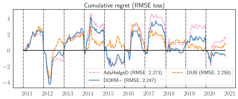
Figure 2: Regret of regularizers: Yearly cumulative regret (in terms of the RMSE loss) for the three regularization strategies for the Temp. 3-4w task.

Fig. 2 shows the yearly regret of the DUB, AdaHedgeD, and DORM+ algorithms. A consistent pattern appears in the yearly regret: DUB has moderate positive regret, AdaHedgeD has both the largest positive and negative regret values, and DORM+ sits between these two extremes. If we examine the weights played by each algorithm (Fig. 3), the weights of DUB and AdaHedgeD appear respectively over- and under-regularized compared to DORM+ (the top model for this task). DUB’s use of the upper bound $\mathbf{b}_{t,F}$ results in a very large regularization setting ($\lambda_{T}=142.881$) and a virtually uniform weight setting. AdaHedgeD’s tighter bound $\delta_{t}$ produces a value for $\lambda_{T}=3.005$ that is two orders of magnitude smaller. However, in this short-horizon forecasting setting, AdaHedgeD’s aggressive plays result in higher average RMSE. By nature of it’s $\lambda_{t}$-free updates, DORM+ produces more moderately regularized plays $\mathbf{w}_{t}$ and negative regret.

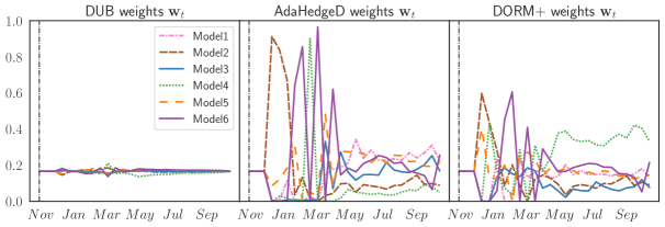
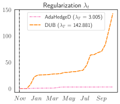
Figure 3: Impact of regularization: The plays $\mathbf{w}_{t}$ of online learning algorithms used to combine the input models for the Temp. 3-4w task in the 2020 evaluation year. The weights of DUB and AdaHedgeD appear respectively over and under regularized compared to DORM+ (the top model for this task) due to their selection of regularization strength $\lambda_{t}$ (right).

To replicate or not to replicate  In this section, we compare the performance of replicated and non-replicated variants of our DORM+ algorithm. Both algorithms perform well (see Sec. M.3), but in all tasks, DORM+ outperforms replicated DORM+ (in which $D+1$ independent copies of DORM+ make staggered predictions). Fig. 4 provides an example of the weight plots produced by the replication strategy in the Temp. 5-6w task with $D=3$. The separate nature of the replicated learner’s plays is evident in the weight plots and leads to an average RMSE of $2.315$, versus $2.303$ for DORM+ in the Temp. 5-6w task.

Figure 4: To replicate or not to replicate: The plays $\mathbf{w}_{t}$ of standard DORM+ and replicated DORM+ algorithms for the Temp. 5-6w task in the final evaluation year.

Learning to hint  Finally, we examine the effect of optimism on the DORM+ algorithms and the ability of our “learning to hint” strategy to recover the performance of the best optimism strategy in retrospect. Following the hint construction protocol in Sec. N.2, we run the DORM+ base algorithm with $m=4$ subgradient hinting strategies: $\tilde{\mathbf{g}}_{s}=\mathbf{g}_{t-D-1}$ (recent_g), $\tilde{\mathbf{g}}_{s}=\mathbf{g}_{s-D-1}$ (prev_g), $\tilde{\mathbf{g}}_{s}=\frac{D+1}{t-D-1}\mathbf{g}_{1:t-D-1}$ (mean_g), or $\tilde{\mathbf{g}}_{s}=\mathbf{0}$ (none). We also use DORM+ as the meta-algorithm for hint learning to produce the learned optimism strategy that plays a convex combination of the four hinters. In Fig. 5, we first note that several optimism strategies outperform the none hinter, confirming the value of optimism in reducing regret. The learned variant of DORM+ avoids the worst-case performance of the individual hinters in any given year (e.g., 2015), while staying competitive with the best strategy (although it does not outperform the dominant recent_g strategy overall). We believe the performance of the online hinter could be further improved by developing tighter convex bounds on the regret of the base problem in the spirit of Assump. 1.

Figure 5: Learning to hint: Yearly cumulative regret (in terms of the RMSE loss) for the adaptive hinting and four constant hinting strategies for the Precip. 3-4w task.

8 Conclusion

In this work, we confronted the challenges of delayed feedback and short regret horizons in online learning with optimism, developing practical non-replicated, self-tuned and tuning-free algorithms with optimal regret guarantees. Our “delay as optimism” reduction and our refined analysis of optimistic learning produced novel regret bounds for both optimistic and delayed online learning and elucidated the connections between these two problems. Within the subseasonal forecasting domain, we demonstrated that delayed online learning methods can produce zero-regret forecast ensembles that perform robustly from year-to-year. Our results highlighted DORM+ as a particularly promising candidate due to its tuning-free nature and small tracking regret.

In future work, we are excited to further develop optimism strategies under delay by 1) employing tighter convex loss bounds on the regret of the base algorithm to improve the learning to hint algorithm, 2) exploring the relative impact of hinting for “past” ($\mathbf{g}_{t-D:t-1}$) versus “future” ($\mathbf{g}_{t}$) missing subgradients (see Sec. M.5 for an initial exploration), and 3) developing adaptive self-tuning variants of the DOOMD algorithm. Within the subseasonal domain, we plan to leverage the flexibility of our optimism formulation to explore hinting strategies that use meteorological expertise to improve beyond the generic mean and past subgradient hints and to deploy our open-source subseasonal forecasting algorithms operationally.

Appendix A Extended Literature Review

We review here additional prior work not detailed in the main paper.

A.1 General online learning

We recommend the monographs of Shalev-Shwartz (2012); Orabona (2019) and the textbook of Cesa-Bianchi & Lugosi (2006) for surveys of the field of online learning and Joulani et al. (2017); McMahan (2017) for widely applicable and modular analyses of online learning algorithms.

A.2 Online learning with optimism but without delay

Syrgkanis et al. (2015) analyzed optimistic FTRL and two-step variant of optimistic MD without delay. The work focuses on a particular form of optimism (using the last observed subgradient as a hint) and shows improved rates of convergence to correlated equilibria in multiplayer games. In the absence of delay, Steinhardt & Liang (2014) combined optimism and adaptivity to obtain improvements over standard optimistic regret bounds.

A.3 Online learning with delay but without optimism

Overview

Joulani et al. (2013, 2016); McMahan & Streeter (2014) provide broad reviews of progress on delayed online learning.

Delayed stochastic optimization

Recht et al. (2011); Agarwal & Duchi (2011); Nesterov (2012); Liu et al. (2014); Liu & Wright (2015); Sra et al. (2016) studied the effects of delay on stochastic optimization but do not treat the adversarial setting studied here.

FTRL-Prox vs. FTRL

Joulani et al. (2016) analyzed the delayed feedback regret of the FTRL-Prox algorithm, which regularizes toward the last played iterate as in online mirror descent, but did not study the standard FTRL algorithms (sometimes called FTRL-Centered) analyzed in this work.

A.4 Self-tuned online learning without delay or optimism

In the absence of optimism and delay, de Rooij et al. (2014); Orabona & Pál (2015); Koolen et al. (2014) developed alternative variants of FTRL algorithms that self-tune their learning rates.

A.5 Online learning without delay for climate forecasting

Monteleoni et al. (2011) applied the Learn-$\alpha$ online learning algorithm of Monteleoni & Jaakkola (2004) to the task of ensembling climate models. The authors considered historical temperature data from 20 climate models and tracked the changing sequence of which model predicts best at any given time. In this context, the algorithm used was based on a set of generalized Hidden Markov Models, in which the identity of the current best model is the hidden variable and the updates are derived as Bayesian updates. This work was extended to take into account the influence of regional neighboring locations when performing updates (McQuade & Monteleoni, 2012). These initial results demonstrated the promise of applying online learning to climate model ensembling, but both methods rely on receiving feedback without delay.

Appendix B Proof of Thm. 3: OFTRL regret

We will prove the following more general result for optimistic adaptive FTRL (OAFTRL)

$$\textstyle\mathbf{w}_{t+1}=\mathop{\mathrm{missing}}{argmin}_{\mathbf{w}\in\mathbf{W}}\,\langle{\mathbf{g}_{1:t}+\tilde{\mathbf{g}}_{t+1}},{\mathbf{w}}\rangle+\lambda_{t+1}\psi(\mathbf{w}),$$ (OAFTRL)

from which Thm. 3 will follow with the choice $\lambda_{t}=\lambda$ for all $t\geq 1$.

Theorem 14 (OAFTRL regret).

If $\psi$ is nonnegative and $(\lambda_{t})_{t\geq 1}$ is non-decreasing, then, $\forall\mathbf{u}\in\mathbf{W}$, the OAFTRL iterates $\mathbf{w}_{t}$ satisfy,

$$\textstyle\textup{Regret}_{T}(\mathbf{u}) \textstyle\leq\lambda_{T}\psi(\mathbf{u})+\sum_{t=1}^{T}\delta_{t}$$ (38)

$$\textstyle\leq\lambda_{T}\psi(\mathbf{u})+\sum_{t=1}^{T}\min\big{(}\frac{1}{\lambda_{t}}\textup{huber}(\|{\mathbf{g}_{t}-\tilde{\mathbf{g}}_{t}}\|_{*},\|{\mathbf{g}_{t}}\|_{*}),\operatorname{diam}({\mathbf{W}})\min(\|{\mathbf{g}_{t}-\tilde{\mathbf{g}}_{t}}\|_{*},\|{\mathbf{g}_{t}}\|_{*})\big{)}$$ (39)

for

$$\textstyle\delta_{t} \textstyle\triangleq\min(F_{t+1}(\mathbf{w}_{t},\lambda_{t})-F_{t+1}(\bar{\mathbf{w}}_{t},\lambda_{t}),\ \ \langle{\mathbf{g}_{t}},{\mathbf{w}_{t}-\bar{\mathbf{w}}_{t}}\rangle,$$ (40)

$$\textstyle\qquad\quad\ F_{t+1}(\hat{\mathbf{w}}_{t},\lambda_{t})-F_{t+1}(\bar{\mathbf{w}}_{t},\lambda_{t})+\langle{\mathbf{g}_{t}},{\mathbf{w}_{t}-\hat{\mathbf{w}}_{t}}\rangle)_{+}\quad\text{with}\quad$$ (41)

$$\textstyle\bar{\mathbf{w}}_{t} \textstyle\triangleq\mathop{\mathrm{missing}}{argmin}_{\mathbf{w}\in\mathbf{W}}F_{t+1}(\mathbf{w},\lambda_{t}),\quad F_{t+1}(\mathbf{w},\lambda_{t})\triangleq\lambda_{t}\psi(\mathbf{w})+\langle{\mathbf{g}_{1:t}},{\mathbf{w}}\rangle,\quad\text{and}\quad$$ (42)

$$\textstyle\hat{\mathbf{w}}_{t} \textstyle\triangleq\mathop{\mathrm{missing}}{argmin}_{\mathbf{w}\in\mathbf{W}}\lambda_{t}\psi(\mathbf{w})+\langle{\mathbf{g}_{1:t}+\min(\frac{\|{\mathbf{g}_{t}}\|_{*}}{\|{\tilde{\mathbf{g}}_{t}-\mathbf{g}_{t}}\|_{*}},1)(\tilde{\mathbf{g}}_{t}-\mathbf{g}_{t})},{\mathbf{w}}\rangle.$$ (43)

Proof.

Consider a sequence of arbitrary auxiliary subgradient hints $\tilde{\mathbf{g}}^{*}_{1},\dots,\tilde{\mathbf{g}}^{*}_{T}\in\mathbb{R}^{d}$ and the auxiliary OAFTRL sequence

$$\textstyle\mathbf{w}^{*}_{t+1}=\mathop{\mathrm{missing}}{argmin}_{\mathbf{w}^{*}\in\mathbf{W}}\,\langle{\mathbf{g}_{1:t}+\tilde{\mathbf{g}}^{*}_{t+1}},{\mathbf{w}^{*}}\rangle+\lambda_{t+1}\psi(\mathbf{w}^{*})\quad\text{for}\quad 0\leq t\leq T\quad\text{with}\quad\tilde{\mathbf{g}}^{*}_{T+1}\triangleq\mathbf{0}\quad\text{and}\quad\lambda_{T+1}=\lambda_{T}.$$ (44)

Generalizing the forward regret decomposition of Joulani et al. (2017) and the prediction drift decomposition of Joulani et al. (2016), we will decompose the regret of our original $(\mathbf{w}_{t})_{t=1}^{T}$ sequence into the regret of the auxiliary sequence $(\mathbf{w}^{*}_{t})_{t=1}^{T}$ and the drift between $(\mathbf{w}_{t})_{t=1}^{T}$ and $(\mathbf{w}^{*}_{t})_{t=1}^{T}$.

For each time $t$, define the auxiliary optimistic objective function $\tilde{F}^{*}_{t}(\mathbf{w})=F_{t}(\mathbf{w})+\langle{\tilde{\mathbf{g}}^{*}_{t}},{\mathbf{w}}\rangle$. Fixing any $\mathbf{u}\in\mathbf{W}$, we have the regret bound

$$\textstyle\textup{Regret}_{T}(\mathbf{u}) \textstyle=\sum_{t=1}^{T}\ell_{t}(\mathbf{w}_{t})-\ell_{t}(\mathbf{u})\leq\sum_{t=1}^{T}\langle{\mathbf{g}_{t}},{\mathbf{w}_{t}-\mathbf{u}}\rangle\quad\text{(since each $\ell_{t}$ is convex with $\mathbf{g}_{t}\in\partial\ell_{t}(\mathbf{w}_{t})$)}\quad$$ (45)

$$\textstyle=\underbrace{\sum_{t=1}^{T}\langle{\mathbf{g}_{t}},{\mathbf{w}_{t}-\mathbf{w}^{*}_{t}}\rangle}_{\textup{drift}}+\underbrace{\sum_{t=1}^{T}\langle{\mathbf{g}_{t}},{\mathbf{w}^{*}_{t}-\mathbf{u}}\rangle}_{\textup{auxiliary regret}}.$$ (46)

To control the drift term we employ the following lemma, proved in Sec. B.1, which bounds the difference between two OAFTRL optimizers with different losses but common regularizers.

Lemma 15 (OAFTRL difference bound).

The OAFTRL and auxiliary OAFTRL iterates 44, $\mathbf{w}_{t}$ and $\mathbf{w}^{*}_{t}$, satisfy

$$\textstyle\|{\mathbf{w}_{t}-\mathbf{w}^{*}_{t}}\|\leq\min(\frac{1}{\lambda_{t}}\|{\tilde{\mathbf{g}}_{t}-\tilde{\mathbf{g}}^{*}_{t}}\|_{*},\operatorname{diam}({\mathbf{W}})).$$ (47)

Letting $a=\operatorname{diam}({\mathbf{W}})\in\mathbb{R}\cup\{\infty\}$, we now bound each drift term summand using the Fenchel-Young inequality for dual norms and Lem. 15:

$$\textstyle\langle{\mathbf{g}_{t}},{\mathbf{w}_{t}-\mathbf{w}^{*}_{t}}\rangle\leq\|{\mathbf{g}_{t}}\|_{*}\|{\mathbf{w}_{t}-\mathbf{w}^{*}_{t}}\|\leq\min\big{(}\frac{1}{\lambda_{t}}\|{\mathbf{g}_{t}}\|_{*}\|{\tilde{\mathbf{g}}_{t}-\tilde{\mathbf{g}}^{*}_{t}}\|_{*},a\|{\mathbf{g}_{t}}\|_{*}\big{)}.$$ (48)

To control the auxiliary regret, we begin by invoking the OAFTRL regret bound of Orabona (2019, proof of Thm. 7.28), the nonnegativity of $\psi$, and the assumption that $(\lambda_{t})_{t\geq 1}$ is non-decreasing:

$$\textstyle\sum_{t=1}^{T}\langle{\mathbf{g}_{t}},{\mathbf{w}^{*}_{t}-\mathbf{u}}\rangle \textstyle\leq\lambda_{T+1}\psi(\mathbf{u})-\lambda_{1}\psi(\mathbf{w}^{*}_{1})+\sum_{t=1}^{T}F_{t+1}(\mathbf{w}^{*}_{t},\lambda_{t})-F_{t+1}(\bar{\mathbf{w}}_{t},\lambda_{t})+(\lambda_{t}-\lambda_{t+1})\psi(\mathbf{w}^{*}_{t+1})$$ (49)

$$\textstyle\leq\lambda_{T+1}\psi(\mathbf{u})-\lambda_{1}\psi(\mathbf{w}^{*}_{1})+\sum_{t=1}^{T}F_{t+1}(\mathbf{w}^{*}_{t},\lambda_{t})-F_{t+1}(\bar{\mathbf{w}}_{t},\lambda_{t}).$$ (50)

We next bound the summands in this expression in two ways. Since $\mathbf{w}^{*}_{t}$ is the minimizer of $\tilde{F}^{*}_{t}$, we may apply the Fenchel-Young inequality for dual norms to conclude that

$$\textstyle F_{t+1}(\mathbf{w}^{*}_{t},\lambda_{t})-F_{t+1}(\bar{\mathbf{w}}_{t},\lambda_{t}) \textstyle=\tilde{F}^{*}_{t}(\mathbf{w}^{*}_{t})+\langle{\mathbf{w}^{*}_{t}},{\mathbf{g}_{t}-\tilde{\mathbf{g}}^{*}_{t}}\rangle-(\tilde{F}^{*}_{t}(\bar{\mathbf{w}}_{t})+\langle{\bar{\mathbf{w}}_{t}},{\mathbf{g}_{t}-\tilde{\mathbf{g}}^{*}_{t}}\rangle)$$ (51)

$$\textstyle\leq\langle{\mathbf{w}^{*}_{t}-\bar{\mathbf{w}}_{t}},{\mathbf{g}_{t}-\tilde{\mathbf{g}}^{*}_{t}}\rangle\leq\|{\mathbf{w}^{*}_{t}-\bar{\mathbf{w}}_{t}}\|\|{\mathbf{g}_{t}-\tilde{\mathbf{g}}^{*}_{t}}\|_{*}\leq a\|{\mathbf{g}_{t}-\tilde{\mathbf{g}}^{*}_{t}}\|_{*}.$$ (52)

Moreover, by Orabona (2019, proof of Thm. 7.28) and the fact that $\bar{\mathbf{w}}_{t}$ minimizes $F_{t+1}(\cdot,\lambda_{t})$ over $\mathbf{W}$,

$$\textstyle F_{t+1}(\mathbf{w}^{*}_{t},\lambda_{t})-F_{t+1}(\bar{\mathbf{w}}_{t},\lambda_{t}) \textstyle\leq\frac{\|{\mathbf{g}_{t}-\tilde{\mathbf{g}}^{*}_{t}}\|_{*}^{2}}{2\lambda_{t}}.$$ (53)

Our collective bounds establish that

$$\textstyle\delta_{t}(\tilde{\mathbf{g}}^{*}_{t}) \textstyle\triangleq F_{t+1}(\mathbf{w}^{*}_{t},\lambda_{t})-F_{t+1}(\bar{\mathbf{w}}_{t},\lambda_{t})+\langle{\mathbf{g}_{t}},{\mathbf{w}_{t}-\mathbf{w}^{*}_{t}}\rangle$$ (54)

$$\textstyle\leq\min(\frac{1}{2\lambda_{t}}\|{\mathbf{g}_{t}-\tilde{\mathbf{g}}^{*}_{t}}\|_{*}^{2},a\|{\mathbf{g}_{t}-\tilde{\mathbf{g}}^{*}_{t}}\|_{*})+\min(\frac{1}{\lambda_{t}}\|{\mathbf{g}_{t}}\|_{*}\|{\tilde{\mathbf{g}}_{t}-\tilde{\mathbf{g}}^{*}_{t}}\|_{*},a\|{\mathbf{g}_{t}}\|_{*})$$ (55)

$$\textstyle\leq\frac{1}{2\lambda_{t}}\|{\mathbf{g}_{t}-\tilde{\mathbf{g}}^{*}_{t}}\|_{*}^{2}+\frac{1}{\lambda_{t}}\|{\mathbf{g}_{t}}\|_{*}\|{\tilde{\mathbf{g}}_{t}-\tilde{\mathbf{g}}^{*}_{t}}\|_{*}.$$ (56)

To obtain an interpretable bound on regret, we will minimize the final expression over all convex combinations $\tilde{\mathbf{g}}^{*}_{t}$ of $\mathbf{g}_{t}$ and $\tilde{\mathbf{g}}_{t}$. The optimal choice is given by

$$\hat{\mathbf{g}}_{t} =\mathbf{g}_{t}+c_{*}(\tilde{\mathbf{g}}_{t}-\mathbf{g}_{t})\quad\text{for}\quad$$ (57)

$$c_{*} \triangleq\textstyle\min(\frac{\|{\mathbf{g}_{t}}\|_{*}}{\|{\tilde{\mathbf{g}}_{t}-\mathbf{g}_{t}}\|_{*}},1)=\displaystyle\mathop{\mathrm{missing}}{argmin}_{c\leq 1,\tilde{\mathbf{g}}^{*}_{t}=\mathbf{g}_{t}+c(\tilde{\mathbf{g}}_{t}-\mathbf{g}_{t})}\textstyle\frac{1}{2\lambda_{t}}\|{\mathbf{g}_{t}-\tilde{\mathbf{g}}^{*}_{t}}\|_{*}^{2}+\frac{1}{\lambda_{t}}\|{\mathbf{g}_{t}}\|_{*}\|{\tilde{\mathbf{g}}_{t}-\tilde{\mathbf{g}}^{*}_{t}}\|_{*}$$ (58)

$$=\textstyle\mathop{\mathrm{missing}}{argmin}_{c\leq 1}\frac{c^{2}}{2\lambda_{t}}\|{\mathbf{g}_{t}-\tilde{\mathbf{g}}_{t}}\|_{*}^{2}+\frac{1-c}{\lambda_{t}}\|{\mathbf{g}_{t}}\|_{*}\|{\tilde{\mathbf{g}}_{t}-\mathbf{g}_{t}}\|_{*}.$$ (59)

For this choice, we obtain the bound

$$\textstyle(\delta_{t}(\hat{\mathbf{g}}_{t}))_{+} \textstyle\leq\frac{1}{2\lambda_{t}}\|{\mathbf{g}_{t}-\hat{\mathbf{g}}_{t}}\|_{*}^{2}+\frac{1}{\lambda_{t}}\|{\mathbf{g}_{t}}\|_{*}\|{\hat{\mathbf{g}}_{t}-\tilde{\mathbf{g}}_{t}}\|_{*}$$ (60)

$$\textstyle=\frac{c_{*}^{2}}{2\lambda_{t}}\|{\mathbf{g}_{t}-\tilde{\mathbf{g}}_{t}}\|_{*}^{2}+\frac{1-c_{*}}{\lambda_{t}}\|{\mathbf{g}_{t}}\|_{*}\|{\mathbf{g}_{t}-\tilde{\mathbf{g}}_{t}}\|_{*}$$ (61)

$$\textstyle=\frac{1}{2\lambda_{t}}\min(\|{\mathbf{g}_{t}-\tilde{\mathbf{g}}_{t}}\|_{*},\|{\mathbf{g}_{t}}\|_{*})^{2}+\frac{1}{\lambda_{t}}\|{\mathbf{g}_{t}}\|_{*}(\|{\mathbf{g}_{t}-\tilde{\mathbf{g}}_{t}}\|_{*}-\|{\mathbf{g}_{t}}\|_{*})_{+}$$ (62)

$$\textstyle=\frac{1}{2\lambda_{t}}(\|{\mathbf{g}_{t}-\tilde{\mathbf{g}}_{t}}\|_{*}^{2}-(\|{\mathbf{g}_{t}-\tilde{\mathbf{g}}_{t}}\|_{*}-\|{\mathbf{g}_{t}}\|_{*})_{+}^{2})$$ (63)

$$\textstyle=\frac{1}{\lambda_{t}}\textup{huber}(\|{\mathbf{g}_{t}-\tilde{\mathbf{g}}_{t}}\|_{*},\|{\mathbf{g}_{t}}\|_{*})$$ (64)

and therefore

$$\textstyle\delta_{t}=\min(\delta_{t}(\tilde{\mathbf{g}}_{t}),\delta_{t}(\mathbf{g}_{t}),\delta_{t}(\hat{\mathbf{g}}_{t}))_{+} \textstyle\leq\min(\frac{1}{\lambda_{t}}\textup{huber}(\|{\mathbf{g}_{t}-\tilde{\mathbf{g}}_{t}}\|_{*},\|{\mathbf{g}_{t}}\|_{*}),a\min(\|{\mathbf{g}_{t}-\tilde{\mathbf{g}}_{t}}\|_{*},\|{\mathbf{g}_{t}}\|_{*})).$$ (65)

Since $\tilde{\mathbf{g}}^{*}_{t}$ is arbitrary, the advertised regret bounds follow as

$$\textstyle\textup{Regret}_{T}(\mathbf{u}) \textstyle\leq\inf_{\tilde{\mathbf{g}}^{*}_{1},\dots,\tilde{\mathbf{g}}^{*}_{T}\in\mathbb{R}^{d}}\lambda_{T+1}\psi(\mathbf{u})+\sum_{t=1}^{T}\delta_{t}(\tilde{\mathbf{g}}^{*}_{t})$$ (66)

$$\textstyle=\lambda_{T+1}\psi(\mathbf{u})+\sum_{t=1}^{T}\inf_{\tilde{\mathbf{g}}^{*}_{t}\in\mathbb{R}^{d}}\delta_{t}(\tilde{\mathbf{g}}^{*}_{t})$$ (67)

$$\textstyle\leq\lambda_{T+1}\psi(\mathbf{u})+\sum_{t=1}^{T}\min(\delta_{t}(\tilde{\mathbf{g}}_{t}),\delta_{t}(\mathbf{g}_{t}),\delta_{t}(\hat{\mathbf{g}}_{t}))_{+}.$$ (68)

∎

B.1 Proof of Lem. 15: OAFTRL difference bound

Fix any time $t$, and define the optimistic objective function $\tilde{F}_{t}(\mathbf{w})=\lambda_{t}\psi(\mathbf{w})+\sum_{i=1}^{t-1}\langle{\mathbf{g}_{i}},{\mathbf{w}}\rangle+\langle{\tilde{\mathbf{g}}_{t}},{\mathbf{w}}\rangle$ and the auxiliary optimistic objective function $\tilde{F}^{*}_{t}(\mathbf{w})=\lambda_{t}\psi(\mathbf{w})+\sum_{i=1}^{t-1}\langle{\mathbf{g}_{i}},{\mathbf{w}}\rangle+\langle{\tilde{\mathbf{g}}^{*}_{t}},{\mathbf{w}}\rangle$ so that $\mathbf{w}_{t}\in\mathop{\mathrm{missing}}{argmin}_{\mathbf{w}\in\mathbf{W}}\tilde{F}_{t}(\mathbf{w})$ and $\mathbf{w}^{*}_{t}\in\mathop{\mathrm{missing}}{argmin}_{\mathbf{w}\in\mathbf{W}}\tilde{F}^{*}_{t}(\mathbf{w})$. We have

$$\textstyle\tilde{F}^{*}_{t}(\mathbf{w}_{t})-\tilde{F}^{*}_{t}(\mathbf{w}^{*}_{t}) \textstyle\geq\frac{\lambda_{t}}{2}\|{\mathbf{w}_{t}-\mathbf{w}^{*}_{t}}\|^{2}\quad\text{by the strong convexity of $\tilde{F}^{*}_{t}$ and}\quad$$ (69)

$$\textstyle\tilde{F}_{t}(\mathbf{w}^{*}_{t})-\tilde{F}_{t}(\mathbf{w}_{t}) \textstyle\geq\frac{\lambda_{t}}{2}\|{\mathbf{w}_{t}-\mathbf{w}^{*}_{t}}\|^{2}\quad\text{by the strong convexity of $\tilde{F}_{t}$.}\quad$$ (70)

Summing the above inequalities and applying the Fenchel-Young inequality for dual norms, we obtain

$$\lambda_{t}\|{\mathbf{w}_{t}-\mathbf{w}^{*}_{t}}\|^{2} \leq\langle{\tilde{\mathbf{g}}^{*}_{t}-\tilde{\mathbf{g}}_{t}},{\mathbf{w}_{t}-\mathbf{w}^{*}_{t}}\rangle\leq\|{\tilde{\mathbf{g}}_{t}-\tilde{\mathbf{g}}^{*}_{t}}\|_{*}\|{\mathbf{w}_{t}-\mathbf{w}^{*}_{t}}\|,$$ (71)

which yields the first half of our target bound after rearrangement. The second half follows from the definition of diameter, as $\|{\mathbf{w}_{t}-\mathbf{w}^{*}_{t}}\|\leq\operatorname{diam}({\mathbf{W}})$.

Appendix C Proof of Thm. 4: SOOMD regret

We will prove the following more general result for adaptive SOOMD (ASOOMD)

$$\mathbf{w}_{t+1}=\mathop{\mathrm{missing}}{argmin}_{\mathbf{w}\in\mathbf{W}}\,\langle{\mathbf{g}_{t}+\tilde{\mathbf{g}}_{t+1}-\tilde{\mathbf{g}}_{t}},{\mathbf{w}}\rangle+\lambda_{t+1}\mathcal{B}_{\psi}(\mathbf{w},\mathbf{w}_{t})\quad\text{with arbitrary}\quad\mathbf{w}_{0}\quad\text{and}\quad\mathbf{g}_{0}=\tilde{\mathbf{g}}_{0}=\mathbf{0}$$ (ASOOMD)

from which Thm. 4 will follow with the choice $\lambda_{t}=\lambda$ for all $t\geq 1$.

Theorem 16 (ASOOMD regret).

Fix any $\lambda_{T+1}\geq 0$. If each $(\lambda_{t+1}-\lambda_{t})\psi$ is proper and differentiable, $\lambda_{0}\triangleq 0$, and $\tilde{\mathbf{g}}_{T+1}\triangleq\mathbf{0}$, then, for all $\mathbf{u}\in\mathbf{W}$, the ASOOMD iterates $\mathbf{w}_{t}$ satisfy

$$\textstyle\textup{Regret}_{T}(\mathbf{u})\leq \textstyle\sum_{t=0}^{T}(\lambda_{t+1}-\lambda_{t})\mathcal{B}_{\psi}(\mathbf{u},\mathbf{w}_{t})+$$ (72)

$$\textstyle\sum_{t=1}^{T}\min\big{(}\operatorname{diam}({\mathbf{W}})\|{\mathbf{g}_{t}-\tilde{\mathbf{g}}_{t}}\|_{*},\frac{1}{\lambda_{t+1}}\textup{huber}(\|{\mathbf{g}_{t}-\tilde{\mathbf{g}}_{t}}\|_{*},\|{\mathbf{g}_{t}+\tilde{\mathbf{g}}_{t+1}-\tilde{\mathbf{g}}_{t}}\|_{*})\big{)}.$$ (73)

Proof.

Fix any $\mathbf{u}\in\mathbf{W}$, instantiate the notation of Joulani et al. (2017, Sec. 7.2), and consider the choices

• $r_{1}=\lambda_{2}\psi$, $r_{t}=(\lambda_{t+1}-\lambda_{t})\psi$ for $t\geq 2$, so that $r_{1:t}=\lambda_{t+1}\psi$ for $t\geq 1$,

• $q_{t}=\tilde{q}_{t}+\langle{\tilde{\mathbf{g}}_{t+1}-\tilde{\mathbf{g}}_{t}},{\cdot}\rangle$ for $t\geq 0$,

• $\tilde{q}_{0}(\mathbf{w})=\lambda_{1}\mathcal{B}_{\psi}(\mathbf{w},\mathbf{w}_{0})$ and $\tilde{q}_{t}\equiv 0$ for all $t\geq 1$,

• $p_{1}\triangleq r_{1}-q_{0}=r_{1}-\tilde{q}_{0}-\langle{\tilde{\mathbf{g}}_{1}-\tilde{\mathbf{g}}_{0}},{\cdot}\rangle=\lambda_{2}\psi-\lambda_{1}\mathcal{B}_{\psi}(\cdot,\mathbf{w}_{0})-\langle{\tilde{\mathbf{g}}_{1}-\tilde{\mathbf{g}}_{0}},{\cdot}\rangle$,

• $p_{t}\triangleq r_{t}-q_{t-1}=r_{t}-\tilde{q}_{t-1}-\langle{\tilde{\mathbf{g}}_{t}-\tilde{\mathbf{g}}_{t-1}},{\cdot}\rangle=(\lambda_{t+1}-\lambda_{t})\psi-\langle{\tilde{\mathbf{g}}_{t}-\tilde{\mathbf{g}}_{t-1}},{\cdot}\rangle$ for all $t\geq 2$.

Since, for each $t$, $\delta_{t}=0$ and $\ell_{t}$ is convex, the Ada-MD regret inequality of Joulani et al. (2017, Eq. (24)) and the choice $\tilde{\mathbf{g}}_{T+1}=0$ imply that

$$\textup{Regret}_{T}(\mathbf{u}) =\sum_{t=1}^{T}\ell_{t}(\mathbf{w}_{t})-\sum_{t=1}^{T}\ell_{t}(\mathbf{u})$$ (74)

$$\leq-\sum_{t=1}^{T}\mathcal{B}_{\ell_{t}}(\mathbf{u},\mathbf{w}_{t})+\sum_{t=0}^{T}q_{t}(\mathbf{u})-q_{t}(\mathbf{w}_{t+1})+\sum_{t=1}^{T}\mathcal{B}_{p_{t}}(\mathbf{u},\mathbf{w}_{t})$$ (75)

$$\quad-\sum_{t=1}^{T}\mathcal{B}_{r_{1:t}}(\mathbf{w}_{t+1},\mathbf{w}_{t})+\sum_{t=1}^{T}\langle{\mathbf{g}_{t}},{\mathbf{w}_{t}-\mathbf{w}_{t+1}}\rangle+\sum_{t=1}^{T}\delta_{t}$$ (76)

$$\leq\lambda_{1}(\mathcal{B}_{\psi}(\mathbf{u},\mathbf{w}_{0})-\mathcal{B}_{\psi}(\mathbf{w}_{1},\mathbf{w}_{0}))+\sum_{t=0}^{T}\langle{\tilde{\mathbf{g}}_{t+1}-\tilde{\mathbf{g}}_{t}},{\mathbf{u}-\mathbf{w}_{t+1}}\rangle$$ (77)

$$\quad+\sum_{t=1}^{T}(\lambda_{t+1}-\lambda_{t})\mathcal{B}_{\psi}(\mathbf{u},\mathbf{w}_{t})+\sum_{t=1}^{T}\langle{\mathbf{g}_{t}},{\mathbf{w}_{t}-\mathbf{w}_{t+1}}\rangle-\lambda_{t+1}\mathcal{B}_{\psi}(\mathbf{w}_{t+1},\mathbf{w}_{t})$$ (78)

$$=\sum_{t=0}^{T}(\lambda_{t+1}-\lambda_{t})\mathcal{B}_{\psi}(\mathbf{u},\mathbf{w}_{t})+\sum_{t=0}^{T}\langle{\mathbf{g}_{t}-\tilde{\mathbf{g}}_{t}},{\mathbf{w}_{t}-\mathbf{w}_{t+1}}\rangle-\lambda_{t+1}\mathcal{B}_{\psi}(\mathbf{w}_{t+1},\mathbf{w}_{t}).$$ (79)

To obtain our advertised bound, we begin with the expression 79 and invoke the $1$-strong convexity of $\psi$ and the nonnegativity of $\mathcal{B}_{\lambda\psi}(\mathbf{w}_{1},\mathbf{w}_{0})$ to find

$$\textstyle\textup{Regret}_{T}(\mathbf{u}) \textstyle\leq\sum_{t=0}^{T}(\lambda_{t+1}-\lambda_{t})\mathcal{B}_{\psi}(\mathbf{u},\mathbf{w}_{t})+\sum_{t=0}^{T}\langle{\mathbf{g}_{t}-\tilde{\mathbf{g}}_{t}},{\mathbf{w}_{t}-\mathbf{w}_{t+1}}\rangle-\lambda_{t+1}\mathcal{B}_{\psi}(\mathbf{w}_{t+1},\mathbf{w}_{t})$$ (80)

$$\textstyle\leq\sum_{t=0}^{T}(\lambda_{t+1}-\lambda_{t})\mathcal{B}_{\psi}(\mathbf{u},\mathbf{w}_{t})+\sum_{t=1}^{T}\langle{\mathbf{g}_{t}-\tilde{\mathbf{g}}_{t}},{\mathbf{w}_{t}-\mathbf{w}_{t+1}}\rangle-\frac{\lambda_{t+1}}{2}\|{\mathbf{w}_{t}-\mathbf{w}_{t+1}}\|^{2}.$$ (81)

We will bound the final sum in this expression using two lemmas. The first is a bound on the difference between subsequent ASOOMD iterates distilled from Joulani et al. (2016, proof of Prop. 2).

Lemma 17 (ASOOMD iterate bound (Joulani et al., 2016, proof of Prop. 2)).

If $\psi$ is differentiable and $1$-strongly convex with respect to $\|{\cdot}\|$, then the ASOOMD iterates satisfy

$$\textstyle\|{\mathbf{w}_{t}-\mathbf{w}_{t+1}}\|\leq\frac{1}{\lambda_{t+1}}\|{\mathbf{g}_{t}+\tilde{\mathbf{g}}_{t+1}-\tilde{\mathbf{g}}_{t}}\|_{*}.$$ (82)

The second, proved in Sec. C.1, is a general bound on $\langle{\mathbf{g}},{\mathbf{v}}\rangle-\frac{\lambda}{2}\|{\mathbf{v}}\|^{2}$ under a norm constraint on $\mathbf{v}$.

Lemma 18 (Norm-constrained conjugate).

For any $\mathbf{g}\in\mathbb{R}^{d}$ and $\lambda,c,b>0$,

$$\sup_{\mathbf{v}\in\mathbb{R}^{d}:\|{\mathbf{v}}\|\leq\min(\frac{c}{\lambda},b)}\textstyle\langle{\mathbf{g}},{\mathbf{v}}\rangle-\frac{\lambda}{2}\|{\mathbf{v}}\|^{2} =\textstyle\frac{1}{\lambda}\min(\|{\mathbf{g}}\|_{*},c,b\lambda)(\|{\mathbf{g}}\|_{*}-\frac{1}{2}\min(\|{\mathbf{g}}\|_{*},c,b\lambda))$$ (83)

$$\leq\textstyle\min(b\|{\mathbf{g}}\|_{*},\frac{1}{\lambda}\min(\|{\mathbf{g}}\|_{*},c)(\|{\mathbf{g}}\|_{*}-\frac{1}{2}\min(\|{\mathbf{g}}\|_{*},c)))$$ (84)

$$=\textstyle\min(b\|{\mathbf{g}}\|_{*},\frac{1}{2\lambda}(\|{\mathbf{g}}\|_{*}^{2}-(\|{\mathbf{g}}\|_{*}-\min(\|{\mathbf{g}}\|_{*},c))^{2}))$$ (85)

$$=\textstyle\min(b\|{\mathbf{g}}\|_{*},\frac{1}{2\lambda}(\|{\mathbf{g}}\|_{*}^{2}-(\|{\mathbf{g}}\|_{*}-c)_{+}^{2}))$$ (86)

$$\leq\textstyle\min(\frac{1}{2\lambda}\|{\mathbf{g}}\|_{*}^{2},\frac{1}{\lambda}c\|{\mathbf{g}}\|_{*},b\|{\mathbf{g}}\|_{*}).$$ (87)

By Lems. 17 and 18 and the definition of $a\triangleq\operatorname{diam}({\mathbf{W}})$, each summand in our regret bound 81 satisfies

$$\langle{\mathbf{g}_{t}-\tilde{\mathbf{g}}_{t}},{\mathbf{w}_{t}-\mathbf{w}_{t+1}}\rangle-\textstyle\frac{\lambda_{t+1}}{2}\|{\mathbf{w}_{t}-\mathbf{w}_{t+1}}\|^{2}\leq\,\displaystyle\sup_{\mathbf{v}\in\mathbb{R}^{d}:\|{\mathbf{v}}\|\leq\min(\frac{1}{\lambda_{t+1}}\|{\mathbf{g}_{t}+\tilde{\mathbf{g}}_{t+1}-\tilde{\mathbf{g}}_{t}}\|_{*},a)}\textstyle\langle{\mathbf{g}_{t}-\tilde{\mathbf{g}}_{t}},{\mathbf{v}}\rangle-\frac{\lambda_{t+1}}{2}\|{\mathbf{v}}\|^{2}$$ (88)

$$=\, \textstyle\min\big{(}a\|{\mathbf{g}_{t}-\tilde{\mathbf{g}}_{t}}\|_{*},\frac{1}{2\lambda_{t+1}}(\|{\mathbf{g}_{t}-\tilde{\mathbf{g}}_{t}}\|_{*}^{2}-(\|{\mathbf{g}_{t}-\tilde{\mathbf{g}}_{t}}\|_{*}-\|{\mathbf{g}_{t}+\tilde{\mathbf{g}}_{t+1}-\tilde{\mathbf{g}}_{t}}\|_{*})_{+}^{2})\big{)}$$ (89)

yielding the advertised result. ∎

C.1 Proof of Lem. 18: Norm-constrained conjugate

By the definition of the dual norm,

$$\sup_{\mathbf{v}\in\mathbb{R}^{d}:\|{\mathbf{v}}\|\leq\min(\frac{c}{\lambda},b)}\textstyle\langle{\mathbf{g}},{\mathbf{v}}\rangle-\frac{\lambda}{2}\|{\mathbf{v}}\|^{2} =\sup_{a\leq\min(\frac{c}{\lambda},b)}\sup_{\mathbf{v}\in\mathbb{R}^{d}:\|{\mathbf{v}}\|\leq a}\textstyle\langle{\mathbf{g}},{\mathbf{v}}\rangle-\frac{\lambda}{2}a^{2}=\displaystyle\sup_{a\leq\min(\frac{c}{\lambda},b)}\textstyle a\|{\mathbf{g}}\|_{*}-\frac{\lambda}{2}a^{2}$$ (90)

$$=\textstyle\frac{1}{\lambda}\min(\|{\mathbf{g}}\|_{*},c,b\lambda)(\|{\mathbf{g}}\|_{*}-\frac{1}{2}\min(\|{\mathbf{g}}\|_{*},c,b\lambda))\leq\min(\frac{1}{\lambda}c\|{\mathbf{g}}\|_{*},b\|{\mathbf{g}}\|_{*}).$$ (91)

We compare to the values of less constrained optimization problems to obtain the final inequalities:

$$\displaystyle\sup_{a\leq\min(\frac{c}{\lambda},b)}\textstyle a\|{\mathbf{g}}\|_{*}-\frac{\lambda}{2}a^{2} \leq\displaystyle\sup_{a\leq\frac{c}{\lambda}}\textstyle a\|{\mathbf{g}}\|_{*}-\frac{\lambda}{2}a^{2}=\textstyle\frac{1}{\lambda}\min(\|{\mathbf{g}}\|_{*},c)(\|{\mathbf{g}}\|_{*}-\frac{1}{2}\min(\|{\mathbf{g}}\|_{*},c))$$ (92)

$$\leq\displaystyle\sup_{a>0}\textstyle a\|{\mathbf{g}}\|_{*}-\frac{\lambda}{2}a^{2}=\frac{1}{\lambda}\frac{1}{2}\|{\mathbf{g}}\|_{*}^{2}.$$ (93)

Appendix D Proof of Lem. 8: DORM is ODAFTRL and DORM + is DOOMD

Our derivations will make use of several facts about $\ell^{p}$ norms, summarized in the next lemma.

Lemma 19 ($\ell^{p}$ norm facts).

For $p\in(1,\infty)$, $\psi(\mathbf{w})=\frac{1}{2}\|{\mathbf{w}}\|_{p}^{2}$, and any vectors $\mathbf{w},\mathbf{v}\in\mathbb{R}^{d}$ and $\tilde{\mathbf{w}}_{0}\in\mathbb{R}_{+}^{d}$,

$$\nabla\psi(\mathbf{w}) =\nabla{\textstyle\frac{1}{2}}\|{\mathbf{w}}\|_{p}^{2}=\mathop{\mathrm{missing}}{sign}(\mathbf{w})|\mathbf{w}|^{p-1}/\|{\mathbf{w}}\|_{p}^{p-2}$$ (94)

$$\langle{\mathbf{w}},{\nabla\psi(\mathbf{w})}\rangle =\|{\mathbf{w}}\|_{p}^{2}=2\psi(\mathbf{w})$$ (95)

$$\psi^{*}(\mathbf{v}) =\sup_{\mathbf{w}\in\mathbb{R}^{d}}\langle{\mathbf{w}},{\mathbf{v}}\rangle-\psi(\mathbf{w})={\textstyle\frac{1}{2}}\|{\mathbf{v}}\|_{q}^{2}\quad\text{for}\quad 1/q=1-1/p$$ (96)

$$\nabla\psi^{*}(\mathbf{v}) =\mathop{\mathrm{missing}}{sign}(\mathbf{v})|\mathbf{v}|^{q-1}/\|{\mathbf{v}}\|_{q}^{q-2}$$ (97)

$$\psi_{+}^{*}(\mathbf{v}) =\sup_{\mathbf{w}\in\mathbb{R}_{+}^{d}}\langle{\mathbf{w}},{\mathbf{v}}\rangle-\psi(\mathbf{w})=\sup_{\mathbf{w}\in\mathbb{R}^{d}}\langle{\mathbf{w}},{(\mathbf{v})_{+}}\rangle-\psi(\mathbf{w})={\textstyle\frac{1}{2}}\|{(\mathbf{v})_{+}}\|_{q}^{2}$$ (98)

$$\nabla\psi_{+}^{*}(\mathbf{v}) =\mathop{\mathrm{missing}}{argmax}_{\mathbf{w}\in\mathbb{R}_{+}^{d}}\langle{\mathbf{w}},{\mathbf{v}}\rangle-\psi(\mathbf{w})=\mathop{\mathrm{missing}}{argmin}_{\mathbf{w}\in\mathbb{R}_{+}^{d}}\psi(\mathbf{w})-\langle{\mathbf{w}},{\mathbf{v}}\rangle=(\mathbf{v})_{+}^{q-1}/\|{(\mathbf{v})_{+}}\|_{q}^{q-2}$$ (99)

$$\min_{\tilde{\mathbf{w}}\in\mathbb{R}_{+}^{d}}\mathcal{B}_{\lambda\psi}(\tilde{\mathbf{w}},\tilde{\mathbf{w}}_{0})-\langle{\mathbf{v}},{\tilde{\mathbf{w}}}\rangle =\lambda(\langle{\tilde{\mathbf{w}}_{0}},{\nabla\psi(\tilde{\mathbf{w}}_{0})}\rangle-\psi(\tilde{\mathbf{w}}_{0})-\sup_{\tilde{\mathbf{w}}\in\mathbb{R}_{+}^{d}}\langle{\tilde{\mathbf{w}}},{\nabla\psi(\tilde{\mathbf{w}}_{0})+\mathbf{v}/\lambda}\rangle-\psi(\tilde{\mathbf{w}}))$$ (100)

$$=\lambda(\langle{\tilde{\mathbf{w}}_{0}},{\nabla\psi(\tilde{\mathbf{w}}_{0})}\rangle-\psi(\tilde{\mathbf{w}}_{0})-\psi_{+}^{*}(\nabla\psi(\tilde{\mathbf{w}}_{0})+\mathbf{v}/\lambda))$$ (101)

$$=\lambda(\psi(\tilde{\mathbf{w}}_{0})-\psi_{+}^{*}(\nabla\psi(\tilde{\mathbf{w}}_{0})+\mathbf{v}/\lambda))$$ (102)

$$=\lambda(\psi(\tilde{\mathbf{w}}_{0})-{\textstyle\frac{1}{2}}\|{(\nabla\psi(\tilde{\mathbf{w}}_{0})+\mathbf{v}/\lambda)_{+}}\|_{q}^{2})$$ (103)

$$=\lambda({\textstyle\frac{1}{2}}\|{\tilde{\mathbf{w}}_{0}}\|_{p}^{2}-{\textstyle\frac{1}{2}}\|{(\tilde{\mathbf{w}}_{0}^{p-1}/\|{\tilde{\mathbf{w}}_{0}}\|_{p}^{p-2}+\mathbf{v}/\lambda)_{+}}\|_{q}^{2}).$$ (104)

Proof.

The fact 94 follows from the chain rule as

$$\textstyle\nabla_{j}\frac{1}{2}\|{\mathbf{w}}\|_{p}^{2} \textstyle=\frac{1}{2}\nabla_{j}(\|{\mathbf{w}}\|_{p}^{p})^{2/p}=\frac{1}{p}(\|{\mathbf{w}}\|_{p}^{p})^{(2/p)-1}\nabla_{j}\|{\mathbf{w}}\|_{p}^{p}=\frac{1}{p}\|{\mathbf{w}}\|_{p}^{2-p}\nabla_{j}\sum_{j^{\prime}=1}^{d}|\mathbf{w}_{j^{\prime}}|^{p}$$ (105)

$$\textstyle=\frac{1}{p}\|{\mathbf{w}}\|_{p}^{2-p}p\mathop{\mathrm{missing}}{sign}(\mathbf{w}_{j})|\mathbf{w}_{j}|^{p-1}=\mathop{\mathrm{missing}}{sign}(\mathbf{w}_{j})|\mathbf{w}_{j}|^{p-1}/\|{\mathbf{w}}\|_{p}^{p-2}.$$ (106)

The fact 96 follows from Lem. 18 as $\|{\cdot}\|_{q}$ is the dual norm of $\|{\cdot}\|_{p}$. ∎

We now prove each claim in turn.

D.1 DORM is ODAFTRL

Fix $p\in(1,2]$, $\lambda>0$, and $t\geq 0$. The ODAFTRL iterate with hint $-\mathbf{h}_{t+1}$, $\mathbf{W}\triangleq\mathbb{R}_{+}^{d}$, $\psi(\tilde{\mathbf{w}})=\frac{1}{2}\|{\tilde{\mathbf{w}}}\|_{p}^{2}$, loss subgradients $\mathbf{g}_{1:t-D}^{\lx@cref{creftype~refnum}{odaftrl}}=-\mathbf{r}_{1:t-D}$, and regularization parameter $\lambda$ takes the form

$$\mathop{\mathrm{missing}}{argmin}_{\tilde{\mathbf{w}}\in\mathbb{R}_{+}^{d}}\ \lambda\psi(\tilde{\mathbf{w}})-\langle{\tilde{\mathbf{w}}},{\mathbf{h}_{t+1}+\mathbf{r}_{1:t-D}}\rangle$$ (107)

$$=\mathop{\mathrm{missing}}{argmin}_{\tilde{\mathbf{w}}\in\mathbb{R}_{+}^{d}}\psi(\tilde{\mathbf{w}})-\langle{\tilde{\mathbf{w}}},{(\mathbf{h}_{t+1}+\mathbf{r}_{1:t-D})/\lambda}\rangle$$ (108)

$$=((\mathbf{r}_{1:t-D}+\mathbf{h}_{t+1})/\lambda)_{+}^{q-1}/\|{((\mathbf{r}_{1:t-D}+\mathbf{h}_{t+1})/\lambda)_{+}}\|_{q}^{q-2}\quad\text{by \lx@cref{creftype~refnum}{argmin_pnorm_reg}}\quad$$ (109)

$$=((\mathbf{r}_{1:t-D}+\mathbf{h}_{t+1})/\lambda)_{+}^{q-1}\|{((\mathbf{r}_{1:t-D}+\mathbf{h}_{t+1})/\lambda)_{+}^{q-1}}\|_{p}^{p-2}\quad\text{since $(p-1)(q-1)=1$}\quad$$ (110)

$$=\tilde{\mathbf{w}}_{t+1}\|{\tilde{\mathbf{w}}_{t+1}}\|_{p}^{p-2}$$ (111)

proving the claim.

D.2 DORM+ is DOOMD

Fix $p\in(1,2]$ and $\lambda>0$, and let $(\tilde{\mathbf{w}}_{t})_{t\geq 0}$ denote the unnormalized iterates generated by DORM+ with hints $\mathbf{h}_{t}$, instantaneous regrets $\mathbf{r}_{t}$, regularization parameter $\lambda$, and hyperparameter $q$. For $p=q/(q-1)$, let $(\bar{\mathbf{w}}_{t})_{t\geq 0}$ denote the sequence generated by DOOMD with $\bar{\mathbf{w}}_{0}=\mathbf{0}$, hints $-\mathbf{h}_{t}$, $\mathbf{W}\triangleq\mathbb{R}_{+}^{d}$, $\psi(\tilde{\mathbf{w}})=\frac{1}{2}\|{\tilde{\mathbf{w}}}\|_{p}^{2}$, loss subgradients $\mathbf{g}_{t}^{\lx@cref{creftype~refnum}{doomd}}=-\mathbf{r}_{t}$, and regularization parameter $\lambda$. We proceed by induction to show that, for each $t$, $\bar{\mathbf{w}}_{t}=\tilde{\mathbf{w}}_{t}\|{\tilde{\mathbf{w}}_{t}}\|_{p}^{p-2}$.

Base case

By assumption, $\bar{\mathbf{w}}_{0}=\mathbf{0}=\tilde{\mathbf{w}}_{0}\|{\tilde{\mathbf{w}}_{0}}\|_{p}^{p-2}$, confirming the base case.

Inductive step

Fix any $t\geq 0$ and assume that for each $s\leq t$, $\bar{\mathbf{w}}_{s}=\tilde{\mathbf{w}}_{s}\|{\tilde{\mathbf{w}}_{s}}\|_{p}^{p-2}$. Then, by the definition of DOOMD and our $\ell^{p}$ norm facts,

$$\bar{\mathbf{w}}_{t+1} =\mathop{\mathrm{missing}}{argmin}_{\bar{\mathbf{w}}\in\mathbb{R}_{+}^{d}}\,\langle{-\mathbf{h}_{t+1}+\mathbf{h}_{t}-\mathbf{r}_{t-D}},{\bar{\mathbf{w}}}\rangle+\mathcal{B}_{\lambda\psi}(\bar{\mathbf{w}},\bar{\mathbf{w}}_{t})$$ (112)

$$=\mathop{\mathrm{missing}}{argmin}_{\bar{\mathbf{w}}\in\mathbb{R}_{+}^{d}}\lambda(\psi(\bar{\mathbf{w}})-\psi(\bar{\mathbf{w}}_{t})-\langle{\bar{\mathbf{w}}-\bar{\mathbf{w}}_{t}},{\nabla\psi(\bar{\mathbf{w}}_{t})}\rangle)+\langle{-\mathbf{h}_{t+1}+\mathbf{h}_{t}-\mathbf{r}_{t-D}},{\bar{\mathbf{w}}}\rangle$$ (113)

$$=\mathop{\mathrm{missing}}{argmin}_{\bar{\mathbf{w}}\in\mathbb{R}_{+}^{d}}\psi(\bar{\mathbf{w}})-\langle{\bar{\mathbf{w}}},{\nabla\psi(\bar{\mathbf{w}}_{t})+(\mathbf{r}_{t-D}-\mathbf{h}_{t}+\mathbf{h}_{t+1})/\lambda}\rangle$$ (114)

$$=\mathop{\mathrm{missing}}{argmin}_{\bar{\mathbf{w}}\in\mathbb{R}_{+}^{d}}\psi(\bar{\mathbf{w}})-\langle{\bar{\mathbf{w}}},{\bar{\mathbf{w}}_{t}^{p-1}/\|{\bar{\mathbf{w}}_{t}}\|_{p}^{p-2}+(\mathbf{r}_{t-D}-\mathbf{h}_{t}+\mathbf{h}_{t+1})/\lambda}\rangle\quad\text{by \lx@cref{creftype~refnum}{grad_pnorm_squared}}\quad$$ (115)

$$=\mathop{\mathrm{missing}}{argmin}_{\bar{\mathbf{w}}\in\mathbb{R}_{+}^{d}}\psi(\bar{\mathbf{w}})-\langle{\bar{\mathbf{w}}},{\tilde{\mathbf{w}}_{t}^{p-1}+(\mathbf{r}_{t-D}-\mathbf{h}_{t}+\mathbf{h}_{t+1})/\lambda}\rangle\quad\text{by the inductive hypothesis}\quad$$ (116)

$$=(\tilde{\mathbf{w}}_{t}^{p-1}+(\mathbf{r}_{t-D}-\mathbf{h}_{t}+\mathbf{h}_{t+1})/\lambda)_{+}^{q-1}/\|{(\tilde{\mathbf{w}}_{t}^{p-1}+(\mathbf{r}_{t-D}-\mathbf{h}_{t}+\mathbf{h}_{t+1})/\lambda)_{+}}\|_{q}^{q-2}\quad\text{by \lx@cref{creftype~refnum}{argmin_pnorm_reg}}\quad$$ (117)

$$=(\tilde{\mathbf{w}}_{t}^{p-1}+(\mathbf{r}_{t-D}-\mathbf{h}_{t}+\mathbf{h}_{t+1})/\lambda)_{+}^{q-1}\|{(\tilde{\mathbf{w}}_{t}^{p-1}+(\mathbf{r}_{t-D}-\mathbf{h}_{t}+\mathbf{h}_{t+1})/\lambda)_{+}^{q-1}}\|_{p}^{p-2}\quad\text{since $(p-1)(q-1)=1$}\quad$$ (118)

$$=\tilde{\mathbf{w}}_{t+1}\|{\tilde{\mathbf{w}}_{t+1}}\|_{p}^{p-2},$$ (119)

completing the inductive step.

Appendix E Proof of Lem. 7: DORM and DORM+ are independent of $\lambda$

We will prove the following more general result, from which the stated result follows immediately.

Lemma 20 (DORM and DORM+ are independent of $\lambda$).

Consider either DORM or DORM+ plays $\tilde{\mathbf{w}}_{t}$ as a function of $\lambda>0$, and suppose that for all time points $t$, the observed subgradient $\mathbf{g}_{t}$ and chosen hint $\mathbf{h}_{t+1}$ only depend on $\lambda$ through $(\mathbf{w}_{s},\lambda^{q-1}\tilde{\mathbf{w}}_{s},\mathbf{g}_{s-1},\mathbf{h}_{s})_{s\leq t}$ and $(\mathbf{w}_{s},\lambda^{q-1}\tilde{\mathbf{w}}_{s},\mathbf{g}_{s},\mathbf{h}_{s})_{s\leq t}$ respectively. Then if $\lambda^{q-1}\tilde{\mathbf{w}}_{0}$ is independent of the choice of $\lambda>0$, then so is $\lambda^{q-1}\tilde{\mathbf{w}}_{t}$ for all time points $t$. As a result, $\mathbf{w}_{t}\propto\lambda^{q-1}\tilde{\mathbf{w}}_{t}$ is also independent of the choice of $\lambda>0$ at all time points.

Proof.

We prove each result by induction on $t$.

E.1 Scaled DORM iterates $\lambda^{q-1}\tilde{\mathbf{w}}_{t}$ are independent of $\lambda$

Base case

By assumption, $\mathbf{h}_{1}$ is independent of the choice of $\lambda>0$. Hence $\lambda^{q-1}\tilde{\mathbf{w}}_{1}=(\mathbf{h}_{1})_{+}^{q-1}$ is independent of $\lambda>0$, confirming the base case.

Inductive step

Fix any $t\geq 0$, suppose $\lambda^{q-1}\tilde{\mathbf{w}}_{s}$ is independent of the choice of $\lambda>0$ for all $s\leq t$, and consider

$$\textstyle\lambda^{q-1}\tilde{\mathbf{w}}_{t+1}=(\mathbf{r}_{1:t-D}+\mathbf{h}_{t+1})_{+}^{q-1}.$$ (120)

Since $\mathbf{r}_{1:t-D}$ depends on $\lambda$ only through $\mathbf{w}_{s}$ and $\mathbf{g}_{s}$ for $s\leq t-D$, our $\lambda$ dependence assumptions for $(\mathbf{g}_{s},\mathbf{h}_{s+1})_{s\leq t}$; the fact that, for each $s$, $\mathbf{w}_{s}\propto\lambda^{q-1}\tilde{\mathbf{w}}_{s}$; and our inductive hypothesis together imply that $\lambda^{q-1}\tilde{\mathbf{w}}_{t+1}$ is independent of $\lambda>0$.

E.2 Scaled DORM+ iterates $\lambda^{q-1}\tilde{\mathbf{w}}_{t}$ are independent of $\lambda$

Base case

By assumption, $\lambda^{q-1}\tilde{\mathbf{w}}_{0}$ is independent of the choice of $\lambda>0$, confirming the base case.

Inductive step

Fix any $t\geq 0$ and suppose $\lambda^{q-1}\tilde{\mathbf{w}}_{s}$ is independent of the choice of $\lambda>0$ for all $s\leq t$. Since $(p-1)(q-1)=1$,

$$\lambda^{q-1}\tilde{\mathbf{w}}_{t+1}=(\lambda\tilde{\mathbf{w}}_{t}^{p-1}+\mathbf{r}_{t-D}-\mathbf{h}_{t}+\mathbf{h}_{t+1})_{+}^{q-1}=((\lambda^{q-1}\tilde{\mathbf{w}}_{t})^{p-1}+\mathbf{r}_{t-D}-\mathbf{h}_{t}+\mathbf{h}_{t+1})_{+}^{q-1}.$$ (121)

Since $\mathbf{r}_{t-D}$ depends on $\lambda$ only through $\mathbf{w}_{t-D}$ and $\mathbf{g}_{t-D}$, our $\lambda$ dependence assumptions for $(\mathbf{g}_{s},\mathbf{h}_{s+1})_{s\leq t}$; the fact that, for each $s\leq t$, $\mathbf{w}_{s}\propto\lambda^{q-1}\tilde{\mathbf{w}}_{s}$; and our inductive hypothesis together imply that $\lambda^{q-1}\tilde{\mathbf{w}}_{t+1}$ is independent of $\lambda>0$. ∎

Appendix F Proof of Cor. 9: DORM and DORM+ regret

Fix any $\lambda>0$ and $\mathbf{u}\in\triangle_{d-1}$, consider the unnormalized DORM or DORM+ iterates $\tilde{\mathbf{w}}_{t}$, and define $\bar{\mathbf{w}}_{t}=\tilde{\mathbf{w}}_{t}\|{\tilde{\mathbf{w}}_{t}}\|_{p}^{p-2}$ for each $t$. For either algorithm, we will bound our regret in terms of the surrogate losses

$$\textstyle\hat{\ell}_{t}(\tilde{\mathbf{w}})\triangleq-\langle{\mathbf{r}_{t}},{\tilde{\mathbf{w}}}\rangle=\langle{\mathbf{g}_{t}},{\tilde{\mathbf{w}}}\rangle-\langle{\tilde{\mathbf{w}}},{\mathbf{1}}\rangle\langle{\mathbf{g}_{t}},{\mathbf{w}_{t}}\rangle$$ (122)

defined for $\tilde{\mathbf{w}}\in\mathbb{R}_{+}^{d}$. Since $\hat{\ell}_{t}(\mathbf{u})=\langle{\mathbf{g}_{t}},{\mathbf{u}-\mathbf{w}_{t}}\rangle$, $\hat{\ell}_{t}(\bar{\mathbf{w}}_{t})=0$, and each $\ell_{t}$ is convex, we have

$$\textstyle\textup{Regret}_{T}(\mathbf{u})=\sum_{t=1}^{T}\ell_{t}(\mathbf{w}_{t})-\ell_{t}(\mathbf{u})\leq\sum_{t=1}^{T}\langle{\mathbf{g}_{t}},{\mathbf{w}_{t}-\mathbf{u}}\rangle=\sum_{t=1}^{T}\hat{\ell}_{t}(\bar{\mathbf{w}}_{t})-\hat{\ell}_{t}(\mathbf{u}).$$ (123)

For DORM, Lem. 8 implies that $(\bar{\mathbf{w}}_{t})_{t\geq 1}$ are ODFTRL iterates, so the ODFTRL regret bound (Thm. 5) and the fact that $\psi$ is $1$-strongly convex with respect to $\|{\cdot}\|=\sqrt{p-1}\|{\cdot}\|_{p}$ (see Shalev-Shwartz, 2007, Lemma 17) with $\|{\cdot}\|_{*}=\frac{1}{\sqrt{p-1}}\|{\cdot}\|_{q}$ imply

$$\textstyle\textup{Regret}_{T}(\mathbf{u})\leq\frac{\lambda}{2}\|{\mathbf{u}}\|_{p}^{2}+\frac{1}{\lambda(p-1)}\sum_{t=1}^{T}\mathbf{b}_{t,q}.$$ (124)

Similarly, for DORM+, Lem. 8 implies that $(\bar{\mathbf{w}}_{t})_{t\geq 0}$ are DOOMD iterates with $\bar{\mathbf{w}}_{0}=\mathbf{0}$, so the DOOMD regret bound (Thm. 6) and the strong convexity of $\psi$ yield

$$\textstyle\textup{Regret}_{T}(\mathbf{u}) \textstyle\leq\mathcal{B}_{\frac{\lambda}{2}\|{\cdot}\|_{p}^{2}}(\mathbf{u},\mathbf{0})+\frac{1}{\lambda(p-1)}\sum_{t=1}^{T}\mathbf{b}_{t,q}=\frac{\lambda}{2}\|{\mathbf{u}}\|_{p}^{2}+\frac{1}{\lambda(p-1)}\sum_{t=1}^{T}\mathbf{b}_{t,q}.$$ (125)

Since, by Lem. 7, the choice of $\lambda$ does not impact the iterate sequences played by DORM and DORM+, we may take the infimum over $\lambda>0$ in these regret bounds. The second advertised inequality comes from the identity $\frac{1}{p-1}=q-1$ and the norm equivalence relations $\|{\mathbf{v}}\|_{q}\leq d^{1/q}\|{\mathbf{v}}\|_{\infty}$ and $\|{\mathbf{v}}\|_{p}\leq\|{\mathbf{v}}\|_{1}=1$ for $\mathbf{v}\in\mathbb{R}^{d}$, as shown in Lem. 21 below. The final claim follows as

$$\textstyle\inf_{q^{\prime}\geq 2}d^{2/q^{\prime}}(q^{\prime}-1)=\inf_{q^{\prime}\geq 2}2^{2\log_{2}(d)/q^{\prime}}(q^{\prime}-1)\leq 2^{2\log_{2}(d)/(2\log_{2}(d))}(2\log_{2}(d)-1)=2(2\log_{2}(d)-1)$$ (126)

since $d>1$.

Lemma 21 (Equivalence of $p$-norms).

If $\mathbf{x}\in\mathbb{R}^{n}$ and $q>q^{\prime}\geq 1$, then $\|{\mathbf{x}}\|_{q}\leq\|{\mathbf{x}}\|_{q^{\prime}}\leq n^{(1/q^{\prime}-1/q)}\|{\mathbf{x}}\|_{q}$.

Proof.

To show $\|\mathbf{x}\|_{q}\leq\|\mathbf{x}\|_{q^{\prime}}$ for $q>q^{\prime}\geq 1$, suppose without loss of generality that $\|\mathbf{x}\|_{q^{\prime}}=1$. Then, $\|\mathbf{x}\|_{q}^{q}=\sum_{i=1}^{n}|x_{i}|^{q}\leq\sum_{i=1}^{n}|x_{i}|^{q^{\prime}}=\|\mathbf{x}\|_{q^{\prime}}^{q^{\prime}}=1$. Hence $\|\mathbf{x}\|_{q}\leq 1=\|\mathbf{x}\|_{q^{\prime}}$.

For the inequality $\|\mathbf{x}\|_{q^{\prime}}\leq n^{1/q^{\prime}-1/q}\|\mathbf{x}\|_{q}$, applying Hölder’s inequality yields

$$\textstyle\|\mathbf{x}\|_{q^{\prime}}^{q^{\prime}}=\sum_{i=1}^{n}1\cdot|x_{i}|^{q^{\prime}}\leq\mathopen{}\mathclose{{}\left(\sum_{i=1}^{n}1}\right)^{1-\frac{q^{\prime}}{q}}\mathopen{}\mathclose{{}\left(\sum_{i=1}^{n}|x_{i}|^{q}}\right)^{\frac{q^{\prime}}{q}}=n^{1-\frac{q^{\prime}}{q}}\|\mathbf{x}\|_{q}^{q^{\prime}},$$ (127)

so $\|\mathbf{x}\|_{q^{\prime}}\leq n^{1/q^{\prime}-1/q}\|\mathbf{x}\|_{q}$. ∎

Appendix G Proof of Thm. 10: ODAFTRL regret

Since ODAFTRL is an instance of OAFTRL with $\tilde{\mathbf{g}}_{t+1}=\mathbf{h}_{t+1}-\sum_{s=t-D+1}^{t}\mathbf{g}_{s}$, the ODAFTRL result follows immediately from the OAFTRL regret bound, Thm. 14.

Appendix H Proof of Thm. 11: DUB Regret

Fix any $\mathbf{u}\in\mathbf{W}$. By Thm. 10, ODAFTRL admits the regret bound

$$\textstyle\textup{Regret}_{T}(\mathbf{u})\leq\lambda_{T}\psi(\mathbf{u})+\sum_{t=1}^{T}\min(\frac{1}{\lambda_{t}}\mathbf{b}_{t,F},\mathbf{a}_{t,F}).$$ (128)

To control the second term in this bound, we apply the following lemma proved in Sec. H.1.

Lemma 22 (DUB-style tuning bound).

Fix any $\alpha>0$ and any non-negative sequences $(a_{t})_{t=1}^{T}$, $(b_{t})_{t=1}^{T}$. If

$$\textstyle\Delta_{t+1}^{*}\triangleq 2\max_{j\leq t-D-1}a_{j-D+1:j}+\sqrt{\sum_{i=1}^{t-D}a_{i}^{2}+2\alpha b_{i}}\leq\alpha\lambda_{t+1}\quad\text{for each}\quad t$$ (129)

then

$$\textstyle\sum_{t=1}^{T}\min(b_{t}^{2}/\lambda_{t},a_{t})\leq\Delta_{T+D+1}^{*}\leq\alpha\lambda_{T+D+1}.$$ (130)

Since $\lambda_{T}\leq\lambda_{T+D+1}$, the result now follows by setting $a_{t}=\mathbf{a}_{t,F}$ and $b_{t}=\mathbf{b}_{t,F}$, so that

$$\textstyle\textup{Regret}_{T}(\mathbf{u})\leq\lambda_{T}\psi(\mathbf{u})+\alpha\lambda_{T+D+1}\leq(\psi(\mathbf{u})+\alpha)\lambda_{T+D+1}.$$ (131)

H.1 Proof of Lem. 22: DUB-style tuning bound

We prove the claim

$$\textstyle\Delta_{t}\triangleq\sum_{i=1}^{t}\min(b_{i}/\lambda_{i},a_{i})\leq\Delta_{t+D+1}^{*}\leq\alpha\lambda_{t+D+1}$$ (132)

by induction on $t$.

Base case

For $t\in[D+1]$,

$$\textstyle\sum_{i=1}^{t}\min(b_{i}/\lambda_{i},a_{i})\leq a_{1:t-1}+a_{t}\leq 2\max_{j\leq t-1}a_{j-D+1:j}+\sqrt{\sum_{i=1}^{t}a_{i}^{2}+2\alpha b_{i}}=\Delta_{t+D+1}^{*}\leq\alpha\lambda_{t+D+1}$$ (133)

confirming the base case.

Inductive step

Now fix any $t+1\geq D+2$ and suppose that

$$\textstyle\Delta_{i}\leq\Delta_{i+D+1}^{*}\leq\alpha\lambda_{i+D+1}$$ (134)

for all $1\leq i\leq t$. We apply this inductive hypothesis to deduce that, for each $0\leq i\leq t$,

$$\Delta_{i+1}^{2}-\Delta_{i}^{2} =\mathopen{}\mathclose{{}\left(\Delta_{i}+\min(b_{i+1}/\lambda_{i+1},a_{i+1})}\right)^{2}-\Delta_{i}^{2}=2\Delta_{i}\min(b_{i+1}/\lambda_{i+1},a_{i+1})+\min(b_{i+1}/\lambda_{i+1},a_{i+1})^{2}$$ (135)

$$=2\Delta_{i-D}\min(b_{i+1}/\lambda_{i+1},a_{i+1})+2(\Delta_{i}-\Delta_{i-D})\min(b_{i+1}/\lambda_{i+1},a_{i+1})+\min(b_{i+1}/\lambda_{i+1},a_{i+1})^{2}$$ (136)

$$=2\Delta_{i-D}\min(b_{i+1}/\lambda_{i+1},a_{i+1})+2\sum_{j=i-D+1}^{i}\min(b_{j}/\lambda_{j},a_{j})\min(b_{i+1}/\lambda_{i+1},a_{i+1})+\min(b_{i+1}/\lambda_{i+1},a_{i+1})^{2}$$ (137)

$$\leq 2\alpha\lambda_{i+1}\min(b_{i+1}/\lambda_{i+1},a_{i+1})+2a_{i-D+1:i}\min(b_{i+1}/\lambda_{i+1},a_{i+1})+a_{i+1}^{2}$$ (138)

$$\leq 2\alpha b_{i+1}+a_{i+1}^{2}+2a_{i-D+1:i}\min(b_{i+1}/\lambda_{i+1},a_{i+1}).$$ (139)

Now, we sum this inequality over $i=0,\dots,t$, to obtain

$$\textstyle\Delta^{2}_{t+1} \textstyle\leq\sum_{i=0}^{t}(2\alpha b_{i+1}+a_{i+1}^{2})+2\sum_{i=0}^{t}a_{i-D+1:i}\min(b_{i+1}/\lambda_{i+1},a_{i+1})$$ (140)

$$\textstyle=\sum_{i=1}^{t+1}(2\alpha b_{i}+a_{i}^{2})+2\sum_{i=1}^{t+1}a_{i-D:i-1}\min(b_{i}/\lambda_{i},a_{i})$$ (141)

$$\textstyle\leq\sum_{i=1}^{t+1}(a_{i}^{2}+2\alpha b_{i})+2\max_{j\leq t}a_{j-D+1:j}\sum_{i=1}^{t+1}\min(b_{i}/\lambda_{i},a_{i})$$ (142)

$$\textstyle=\sum_{i=1}^{t+1}(a_{i}^{2}+2\alpha b_{i})+2\Delta_{t+1}\max_{j\leq t}a_{j-D+1:j}.$$ (143)

Solving this quadratic inequality and applying the triangle inequality, we have

$$\textstyle\Delta_{t+1} \textstyle\leq\max_{j\leq t}a_{j-D+1:j}+\frac{1}{2}\sqrt{(2\max_{j\leq t}a_{j-D+1:j})^{2}+4\sum_{i=1}^{t+1}a_{i}^{2}+2\alpha b_{i}}$$ (144)

$$\textstyle\leq 2\max_{j\leq t}a_{j-D+1:j}+\sqrt{\sum_{i=1}^{t+1}a_{i}^{2}+2\alpha b_{i}}=\Delta_{t+D+2}^{*}\leq\alpha\lambda_{t+D+2}.$$ (145)

Appendix I Proof of Thm. 12: AdaHedgeD Regret

Fix any $\mathbf{u}\in\mathbf{W}$. Since the AdaHedgeD regularization sequence $(\lambda_{t})_{t\geq 1}$ is non-decreasing, Thm. 14 gives the regret bound

$$\textstyle\textup{Regret}_{T}(\mathbf{u}) \textstyle\leq\lambda_{T}\psi(\mathbf{u})+\sum_{t=1}^{T}\delta_{t}=\lambda_{T}\psi(\mathbf{u})+\alpha\lambda_{T+D+1}\leq(\psi(\mathbf{u})+\alpha)\lambda_{T+D+1},$$ (146)

and the proof of Thm. 14 gives the upper estimate 65:

$$\textstyle\delta_{t}\leq\min\Big{(}\frac{\mathbf{b}_{t,F}}{\lambda_{t}},\mathbf{a}_{t,F}\Big{)}\quad\text{for all}\quad t\in[T].$$ (147)

Hence, it remains to bound $\lambda_{T+D+1}$. Since $\lambda_{1}=\dots=\lambda_{D+1}=0$ and $\alpha(\lambda_{t+1}-\lambda_{t})=\delta_{t-D}$ for $t\geq D+1$,

$$\textstyle\alpha\lambda_{T+D+1}^{2} \textstyle=\sum_{t=1}^{T+D}\alpha(\lambda_{t+1}^{2}-\lambda_{t}^{2})=\sum_{t=D+1}^{T+D}\mathopen{}\mathclose{{}\left(\alpha(\lambda_{t+1}-\lambda_{t})^{2}+2\alpha(\lambda_{t+1}-\lambda_{t})\lambda_{t}}\right)$$ (148)

$$\textstyle=\sum_{t=1}^{T}\mathopen{}\mathclose{{}\left(\delta_{t}^{2}/\alpha+2\delta_{t}\lambda_{t+D}}\right)\quad\text{by the definition of $\lambda_{t+1}$}\quad$$ (149)

$$\textstyle=\sum_{t=1}^{T}\mathopen{}\mathclose{{}\left(\delta_{t}^{2}/\alpha+2\delta_{t}\lambda_{t}+2\delta_{t}(\lambda_{t+D}-\lambda_{t})}\right)$$ (150)

$$\textstyle\leq\sum_{t=1}^{T}\mathopen{}\mathclose{{}\left(\delta_{t}^{2}/\alpha+2\delta_{t}\lambda_{t}+2\delta_{t}\max_{t\in[T]}(\lambda_{t+D}-\lambda_{t})}\right)$$ (151)

$$\textstyle=\sum_{t=1}^{T}\mathopen{}\mathclose{{}\left(\delta_{t}^{2}/\alpha+2\delta_{t}\lambda_{t}}\right)+2\lambda_{T+D+1}\max_{t\in[T]}\delta_{t-D:t-1}$$ (152)

$$\textstyle\leq\sum_{t=1}^{T}\mathopen{}\mathclose{{}\left(\mathbf{a}_{t,F}^{2}/\alpha+2\mathbf{b}_{t,F}}\right)+2\lambda_{T+D+1}\max_{t\in[T]}\mathbf{a}_{t-D:t-1,F}\quad\text{by \lx@cref{creftype~refnum}{delta_a_b_bound}.}\quad$$ (153)

Solving the above quadratic inequality for $\lambda_{T+D+1}$ and applying the triangle inequality, we find

$$\textstyle\alpha\lambda_{T+D+1} \textstyle\leq\max_{t\in[T]}\mathbf{a}_{t-D:t-1,F}+\frac{1}{2}\sqrt{4(\max_{t\in[T]}\mathbf{a}_{t-D:t-1,F})^{2}+4\sum_{t=1}^{T}\mathbf{a}_{t,F}^{2}+2\alpha\mathbf{b}_{t,F}}$$ (154)

$$\textstyle\leq 2\max_{t\in[T]}\mathbf{a}_{t-D:t-1,F}+\sqrt{\sum_{t=1}^{T}\mathbf{a}_{t,F}^{2}+2\alpha\mathbf{b}_{t,F}}.$$ (155)

Appendix J Proof of Thm. 13: Learning to hint regret

We begin by bounding the hinting problem regret. Since DORM+ is used for the hinting problem, the following result is an immediate corollary of Cor. 9.

Corollary 23 (DORM+ hinting problem regret).

With convex losses $l_{t}(\omega)=f_{t}(H_{t}\omega)$ and no meta-hints, the DORM+ hinting problem iterates $\omega_{t}$ satisfy, for each $v\in\triangle_{m-1}$,

$$\textstyle\textup{HintRegret}_{T}(v) \textstyle\triangleq\sum_{t=1}^{T}l_{t}(\omega_{t})-\sum_{t=1}^{T}l_{t}(v)\leq\sqrt{\frac{m^{2/q}(q-1)}{2}\sum_{t=1}^{T}\beta_{t,\infty}}\quad\text{for}\quad$$ (156)

$$\textstyle\beta_{t,\infty} \textstyle=\begin{cases}\textup{huber}(\|{\sum_{s=t-D}^{t}\rho_{s}}\|_{\infty},\|{\rho_{t-D}}\|_{\infty}),&\text{for }t<T\\ \frac{1}{2}\|{\sum_{s=t-D}^{t}\rho_{s}}\|_{\infty}^{2},&\text{for }t=T\end{cases}$$ (157)

$$\textstyle\quad\text{where}\quad\rho_{t} \textstyle\triangleq\mathbf{1}\langle{\gamma_{t}},{\omega_{t}}\rangle-\gamma_{t}\quad\text{for}\quad\gamma_{t}\in\partial l_{t}(\omega_{t})\quad\text{is the \emph{instantaneous hinting problem regret}.}\quad$$ (158)

If, in addition, $q=\mathop{\mathrm{missing}}{argmin}_{q^{\prime}\geq 2}m^{2/q^{\prime}}(q^{\prime}-1)$, then $\textup{HintRegret}_{T}(v)\leq\sqrt{(2\log_{2}(m)-1)\sum_{t=1}^{T}\beta_{t,\infty}}$.

Our next lemma, proved in Sec. J.1, provides an interpretable bound for each $\beta_{t,\infty}$ term in terms of the hinting problem subgradients $(\gamma_{t})_{t\geq 1}$.

Lemma 24 (Hinting problem subgradient regret bound).

Under the notation and assumptions of Cor. 23,

$$\textstyle\beta_{t,\infty} \textstyle\leq\begin{cases}\textup{huber}(\xi_{t},\zeta_{t})&\text{if }t<T\\ \frac{1}{2}\xi_{t}&\text{if }t=T\end{cases},\quad\text{for}\quad$$ (159)

$$\textstyle\xi_{t} \textstyle\triangleq 4(D+1)\sum_{s=t-D}^{t}\|{\gamma_{s}}\|_{\infty}^{2}\quad\text{and}\quad$$ (160)

$$\textstyle\zeta_{t} \textstyle\triangleq 4\|{\gamma_{t-D}}\|_{\infty}\sum_{s=t-D}^{t}\|{\gamma_{s}}\|_{\infty}.$$ (161)

Now fix any $\mathbf{u}\in\mathbf{W}$. We invoke Assump. 1, Cor. 23, and Lem. 24 in turn to bound the base problem regret

$$\textstyle\textup{Regret}_{T}(\mathbf{u}) \textstyle=\sum_{t=1}^{T}\ell_{t}(\mathbf{w}_{t})-\ell_{t}(\mathbf{u})$$ (162)

$$\textstyle\leq C_{0}(\mathbf{u})+C_{1}(\mathbf{u})\sqrt{\sum_{t=1}^{T}f_{t}(\mathbf{h}_{t}(\omega_{t}))}\quad\text{by \lx@cref{creftype~refnum}{base_assumptions}}\quad$$ (163)

$$\textstyle\leq C_{0}(\mathbf{u})+C_{1}(\mathbf{u})\sqrt{\inf_{v\in\mathbf{V}}\sum_{t=1}^{T}f_{t}(\mathbf{h}_{t}(v))+\sqrt{(2\log_{2}(m)-1)\sum_{t=1}^{T}\beta_{t,\infty}}}\quad\text{by \lx@cref{creftype~refnum}{dorm+_hinting_regret}}\quad$$ (164)

$$\textstyle\leq C_{0}(\mathbf{u})+C_{1}(\mathbf{u})\sqrt{\inf_{v\in\mathbf{V}}\sum_{t=1}^{T}f_{t}(\mathbf{h}_{t}(v))+\sqrt{(2\log_{2}(m)-1)(\frac{1}{2}\xi_{T}+\sum_{t=1}^{T-1}\textup{huber}(\xi_{t},\zeta_{t}))}}\quad\text{by \lx@cref{creftype~refnum}{beta-bound-general}.}\quad$$ (165)

The advertised bound now follows from the triangle inequality.

J.1 Proof of Lem. 24: Hinting problem subgradient regret bound

Fix any $t\in[T]$. The triangle inequality implies that

$$\textstyle\|{\rho_{t}}\|_{\infty}=\|{\gamma_{t}-\mathbf{1}\langle{\omega_{t}},{\gamma_{t}}\rangle}\|_{\infty}\leq\|{\gamma_{t}}\|_{\infty}+|\langle{\omega_{t}},{\gamma_{t}}\rangle|\leq 2\|{\gamma_{t}}\|_{\infty}$$ (166)

since $\omega_{t}\in\triangle_{m-1}$. We repeatedly apply this finding in conjunction with Jensen’s inequality to conclude

$$\textstyle\|{\sum_{s=t-D}^{t}\rho_{s}}\|_{\infty}^{2} \textstyle\leq(D+1)\sum_{s=t-D}^{t}\|{\rho_{s}}\|_{\infty}^{2}\leq 4(D+1)\sum_{s=t-D}^{t}\|{\gamma_{s}}\|_{\infty}^{2}\quad\text{and}\quad$$ (167)

$$\textstyle\|{\rho_{t-D}}\|_{\infty}\|{\sum_{s=t-D}^{t}\rho_{s}}\|_{\infty} \textstyle\leq\|{\rho_{t-D}}\|_{\infty}\sum_{s=t-D}^{t}\|{\rho_{s}}\|_{\infty}\leq 4\|{\gamma_{t-D}}\|_{\infty}\sum_{s=t-D}^{t}\|{\gamma_{s}}\|_{\infty}.$$ (168)

Appendix K Examples: Learning to Hint with DORM+ and AdaHedgeD

By Thm. 12, AdaHedgeD satisfies Assump. 1 with $f_{t}(\mathbf{h}_{t})=\|{\mathbf{r}_{t}}\|_{*}\|{\mathbf{h}_{t}-\sum_{s=t-D}^{t}\mathbf{r}_{s}}\|_{*}\geq\frac{\mathbf{a}_{t,F}^{2}+2\alpha\mathbf{b}_{t,F}}{\operatorname{diam}({\mathbf{W}})^{2}+2\alpha}$, $C_{1}(\mathbf{u})=\sqrt{\operatorname{diam}({\mathbf{W}})^{2}+2\alpha}$, and $C_{0}(\mathbf{u})=2\operatorname{diam}({\mathbf{W}})\max_{t\in[T]}\sum_{s=t-D}^{t-1}\|{\mathbf{g}_{s}}\|_{*}$.

By Cor. 9, DORM+ satisfies Assump. 1 with $f_{t}(\mathbf{h})=\|{\mathbf{r}_{t-D}+\mathbf{h}_{t+1}-\mathbf{h}_{t}}\|_{q}\|{\mathbf{h}-\sum_{s=t-D}^{t}\mathbf{r}_{s}}\|_{q}$, $C_{0}(\mathbf{u})=0$, and $C_{1}(\mathbf{u})=\sqrt{\frac{\|{\mathbf{u}}\|_{p}^{2}}{2(p-1)}}$.

These choices give rise to the hinting losses

$$\textstyle l_{t}^{\lx@cref{creftype~refnum}{dorm+}}(\omega) \textstyle=\|{\mathbf{r}_{t-D}+\mathbf{h}_{t+1}-\mathbf{h}_{t}}\|_{q}\|{H_{t}\omega-\sum_{s=t-D}^{t}\mathbf{r}_{s}}\|_{q}\quad\text{and}\quad$$ (169)

$$\textstyle l_{t}^{\lx@cref{creftype~refnum}{adahedged}}(\omega) \textstyle=\|{\mathbf{g}_{t}}\|_{q}\|{H_{t}\omega-\sum_{s=t-D}^{t}\mathbf{g}_{s}}\|_{q}\quad\text{when}\quad\|{\cdot}\|_{*}=\|{\cdot}\|_{q}\quad\text{for}\quad q\in[1,\infty].$$ (170)

The following lemma, proved in Sec. K.1, identifies subgradients of these hinting losses.

Lemma 25 (Hinting loss subgradient).

If $l_{t}(\omega)=\|{\bar{\mathbf{g}}_{t}}\|_{q}\|{H_{t}\omega-\mathbf{v}_{t}}\|_{q}$ for some $\bar{\mathbf{g}}_{t},\mathbf{v}_{t}\in\mathbb{R}^{d}$ and $H_{t}\in\mathbb{R}^{d\times m}$, then

$$\gamma_{t}=\begin{cases}\frac{\|{\bar{\mathbf{g}}_{t}}\|_{q}}{\|{H_{t}\omega-\mathbf{v}_{t}}\|_{q}^{q-1}}H_{t}^{\top}|H_{t}\omega-\mathbf{v}_{t}|^{q-1}\mathop{\mathrm{missing}}{sign}(H_{t}\omega-\mathbf{v}_{t})&\text{if }q<\infty\\ \|{\bar{\mathbf{g}}_{t}}\|_{\infty}\mathop{\mathrm{missing}}{sign}(\mu)H_{t}^{\top}\mathbf{e}_{k}&\text{if }q=\infty\end{cases}\quad\in\quad\partial l_{t}(\omega)$$ (171)

for $k=\mathop{\mathrm{missing}}{argmax}_{j\in[d]}(H_{t}\omega-\mathbf{v}_{t})_{j}$ and $\mu=\max_{j\in[d]}(H_{t}\omega-\mathbf{v}_{t})_{j}$.

Our next lemma, proved in Sec. K.2, bounds the $\infty$-norm of this hinting loss subgradient in terms of the base problem subgradients.

Lemma 26 (Hinting loss subgradient bound).

Under the assumptions and notation of Lem. 25, the subgradient $\gamma_{t}$ satisfies $\|{\gamma_{t}}\|_{\infty}\leq d^{1/q}\|{\bar{\mathbf{g}}_{t}}\|_{q}\|{H_{t}}\|_{\infty}$ for $\|{H_{t}}\|_{\infty}$ the maximum absolute entry of $H_{t}$.

K.1 Proof of Lem. 25: Hinting loss subgradient

The result follows immediately from the chain rule and the following lemma.

Lemma 27 (Subgradients of $p$-norms).

Suppose $\mathbf{w}\in\mathbb{R}^{d}$ and $k\in\mathop{\mathrm{missing}}{argmax}_{j\in[d]}|\mathbf{w}_{j}|$. Then

$$\textstyle\partial\|{\mathbf{w}}\|_{p}\ni\begin{cases}\frac{|\mathbf{w}|^{p-1}}{\|{\mathbf{w}}\|_{p}^{p-1}}\mathop{\mathrm{missing}}{sign}(\mathbf{w})&\text{if $\|{\mathbf{w}}\|_{p}\neq 0,p\in[1,\infty)$}\\ \mathbf{e}_{k}\mathop{\mathrm{missing}}{sign}(\mathbf{w}_{k})&\text{if $\|{\mathbf{w}}\|_{p}\neq 0,p=\infty$}\\ \mathbf{0}&\text{if $\|{\mathbf{w}}\|_{p}=0$}\end{cases}.$$ (172)

Proof.

Since $\mathbf{0}$ is a minimizer of $\|{\cdot}\|_{p}$, we have $\|{\mathbf{u}}\|_{p}\geq\|{\mathbf{0}}\|_{p}+\langle{\mathbf{0}},{\mathbf{u}-\mathbf{0}}\rangle$ for any $\mathbf{u}\in\mathbb{R}^{d}$ and hence $\mathbf{0}\in\partial\|{\mathbf{0}}\|_{p}$.

For $p\in[1,\infty)$, by the chain rule, if $\|{\mathbf{w}}\|_{p}\neq\mathbf{0}$,

$$\textstyle\partial_{j}\|{\mathbf{w}}\|_{p} \textstyle=\partial_{j}\big{(}\sum_{k=1}^{n}|\mathbf{w}_{k}|^{p}\big{)}^{1/p}=\frac{1}{p}\big{(}\sum_{k=1}^{n}|\mathbf{w}_{k}|^{p}\big{)}^{(1/p)-1}p|\mathbf{w}_{j}|^{p-1}\mathop{\mathrm{missing}}{sign}(\mathbf{w}_{j})$$ (173)

$$\textstyle=\Big{(}\big{(}\sum_{k=1}^{n}|\mathbf{w}_{k}|^{p}\big{)}^{1/p}\Big{)}^{-(p-1)}|\mathbf{w}_{j}|^{p-1}\mathop{\mathrm{missing}}{sign}(\mathbf{w}_{j})$$ (174)

$$\textstyle=\Big{(}\frac{|\mathbf{w}_{j}|}{\|{\mathbf{w}}\|_{p}}\Big{)}^{p-1}\mathop{\mathrm{missing}}{sign}(\mathbf{w}_{j}).$$ (175)

For $p=\infty$, we have that $\|{\mathbf{w}}\|_{\infty}=\max_{j\in[n]}|\mathbf{w}_{j}|$. By the Danskin-Bertsekas Theorem (Danskin, 2012) for subdifferentials, $\partial\|{\mathbf{w}}\|_{\infty}=\mathop{\mathrm{missing}}{conv}\{\cup\partial|\mathbf{w}_{j}|\quad\text{s.t.}\quad|\mathbf{w}_{j}|=\|{\mathbf{w}}\|_{\infty}\}=\mathop{\mathrm{missing}}{conv}\{\cup\mathop{\mathrm{missing}}{sign}(\mathbf{w}_{j})\mathbf{e}_{j}\quad\text{s.t.}\quad|\mathbf{w}_{j}|=\|{\mathbf{w}}\|_{\infty}\}$, where $\mathop{\mathrm{missing}}{conv}$ is the convex hull operation. ∎

K.2 Proof of Lem. 26: Hinting loss subgradient bound

If $q\in[1,\infty)$, we have

$$\textstyle\|{\gamma_{t}}\|_{\infty} \textstyle=\mathopen{}\mathclose{{}\left\lVert\frac{\|{\bar{\mathbf{g}}_{t}}\|_{q}}{\|{H_{t}\omega-\sum_{s=t-D}^{t}\mathbf{g}_{s}}\|_{q}^{q-1}}H_{t}^{\top}|H_{t}\omega-\sum_{s=t-D}^{t}\mathbf{g}_{s}|^{q-1}\mathop{\mathrm{missing}}{sign}(H_{t}\omega-\sum_{s=t-D}^{t}\mathbf{g}_{s})}\right\rVert_{\infty}$$ (176)

$$\textstyle\leq\frac{\|{\bar{\mathbf{g}}_{t}}\|_{q}\max_{j\in[d]}\|{H_{t}\mathbf{e}_{j}}\|_{q}}{\|{H_{t}\omega-\sum_{s=t-D}^{t}\mathbf{g}_{s}}\|_{q}^{q-1}}\|{H_{t}\omega-\sum_{s=t-D}^{t}\mathbf{g}_{s}}\|_{q}^{q-1}\quad\text{by H\"{o}lder's inequality for $(q,p)$}\quad$$ (177)

$$\textstyle\leq d^{1/q}\|{\bar{\mathbf{g}}_{t}}\|_{q}\|{H_{t}}\|_{\infty}\quad\text{ by \lx@cref{creftype~refnum}{norm-equality}.}\quad$$ (178)

If $q=\infty$, we have

$$\textstyle\|{\gamma_{t}}\|_{\infty}=\mathopen{}\mathclose{{}\left\lVert\|{\bar{\mathbf{g}}_{t}}\|_{\infty}\mathop{\mathrm{missing}}{sign}(\mu)H_{t}^{\top}\mathbf{e}_{k}}\right\rVert_{\infty}=\mathbb{I}\mathopen{}\mathclose{{}\left[{\mu\neq 0}}\right]\|{\bar{\mathbf{g}}_{t}}\|_{\infty}\|{H_{t}}\|_{\infty}\leq d^{1/q}\|{\bar{\mathbf{g}}_{t}}\|_{\infty}\|{H_{t}}\|_{\infty}.$$ (179)

Appendix L Experiment Details

L.1 Subseasonal Forecasting Application

We apply the online learning techniques developed in this paper to the problem of adaptive ensembling for subseasonal weather forecasting. Subseasonal forecasting is the problem predicting meteorological variables, often temperature and precipitation, 2-6 weeks in advance. These mid-range forecasts are critical for managing water resources and mitigating wildfires, droughts, floods, and other extreme weather events (Hwang et al., 2019). However, the subseasonal forecasting task is notoriously difficult due to the joint influences of short-term initial conditions and long-term boundary conditions (White et al., 2017).

To improve subseasonal weather forecasting capabilities, the US Department of Reclamation launched the Sub-Seasonal Climate Forecast Rodeo competition (Nowak et al., 2020), a yearlong real-time forecasting competition for the Western United States. Our experiments are based on Flaspohler et al. (2021), a snapshot of public subseasonal model forecasts including both physics-based and machine learning models. These models were developed for the subseasonal forecasting challenge and make semimonthly forecasts for the contest period (19 October 2019 – 29 September 2020).

To expand our evaluation beyond the subseasonal forecasting competition, we used the forecasts in Flaspohler et al. (2021) for analogous yearlong periods (26 semi-monthly dates starting from the last Wednesday in October) beginning in Oct. 2010 and ending in Sep. 2020. Throughout, we refer to the yearlong period beginning in Oct. 2010 – Sep. 2011 as the 2011 year and so on for each subsequent year. For each forecast date $t$, the models in Flaspohler et al. (2021) were trained only on data available at time $t$ and model hyper-parameters were tuned to optimize average RMSE loss on the 3-year period preceding the forecast date $t$. For a few of the forecast dates, one or more models had missing forecasts; only dates for which all models have forecasts were used in evaluation.

L.2 Problem Definition

Denote the set of $d=6$ input models $\{\mathcal{M}_{1},\dots\mathcal{M}_{d}\}$ with labels: llr (Model1), multillr (Model2), tuned_catboost (Model3), tuned_cfsv2 (Model4), tuned_doy (Model5) and tuned_salient_fri (Model6). On each semimonthly forecast date, each model $\mathcal{M}_{i}$ makes a prediction for each of two meteorological variables (cumulative precipitation and average temperature over 14 days) and two forecasting horizons (3-4 weeks and 5-6 weeks). For the 3-4 week and 5-6 horizons respectively, the forecaster experiences a delay of $D=2$ and $D=3$ forecasts. Each model makes a total of $T=26$ semimonthly forecasts for these four tasks.

At each time $t$, each input model $\mathcal{M}_{i}$ produces a prediction at $G=514$ gridpoints in the Western United States: $\mathbf{x}^{c}_{t,i}\in\mathbb{R}^{G}=\mathcal{M}_{i}(t)$ for task $c$ at time $t$. Let $\mathbf{X}^{c}_{t}\in\mathbb{R}^{G\times d}$ be the matrix containing each input model’s predictions as columns. The true meterological outcome for task $c$ is $\mathbf{y}_{t}^{c}\in\mathbb{R}^{G}$. As online learning is performed for each task separately, we drop the task superscript $c$ in the following.

At each timestep, the online learner makes a forecast prediction $\hat{\mathbf{y}}_{t}$ by playing $\mathbf{w}_{t}\in\mathbf{W}=\triangle_{d-1}$, corresponding to a convex combination of the individual models: $\hat{\mathbf{y}}_{t}=\mathbf{X}_{t}\mathbf{w}_{t}$. The learner then incurs a loss for the play $\mathbf{w}_{t}$ according to the root mean squared (RMSE) error over the geography of interest:

$$\ell_{t}(\mathbf{w}_{t}) =\frac{1}{\sqrt{G}}\mathopen{}\mathclose{{}\left\|\mathbf{y}_{t}-\mathbf{X}_{t}\mathbf{w}_{t}}\right\|_{2},$$ (180)

$$\partial\ell_{t}(\mathbf{w}_{t}) \ni\mathbf{g}_{t}=\begin{cases}\frac{\mathbf{X}_{t}^{\top}(\mathbf{X}_{t}\mathbf{w}_{t}-\mathbf{y}_{t})}{\sqrt{G}\mathopen{}\mathclose{{}\left\|\mathbf{X}_{t}\mathbf{w}_{t}-\mathbf{y}_{t}}\right\|_{2}}&\quad\text{if}\quad\mathbf{X}_{t}\mathbf{w}_{t}-\mathbf{y}_{t}\neq\mathbf{0}\\ \mathbf{0}&\quad\text{if}\quad\mathbf{X}_{t}\mathbf{w}_{t}-\mathbf{y}_{t}=\mathbf{0}\end{cases}$$ (181)

Our objective for the subseasonal forecasting application is to produce an adaptive ensemble forecast that competes with the best input model over the yearlong period. Hence, in our evaluation, we take the competitor set to be the set of individual models $\mathbf{U}=\{\mathbf{e}_{i}:i\in[d]\}$.

Appendix M Extended Experimental Results

We present complete experimental results for the four experiments presented in the main paper (see Sec. 7).

M.1 Competing with the Best Input Model

Results for our three delayed online learning algorithms — DORM, DORM+, and AdaHedgeD— on the four subseasonal prediction tasks for the four optimism strategies described in Sec. 7 (recent_g, prev_g, mean_g, none) are presented below. Each table and figure shows the average RMSE loss and the annual regret versus the best input model in any given year respectively for each algorithm and task.

DORM+ is a competitive model for all three hinting strategies and under the recent_g hinting strategy achieves negative regret on all tasks except Temp. 5-6w. For the Temp. 5-6w task, no online learning model outperforms the best input model for any hinting strategy. For the precipitation tasks, the online learning algorithms presented achieve negative regret using all three hinting strategies for all four tasks. Within the subseasonal forecasting domain, precipitation is often considered a more challenging forecasting task than temperature (White et al., 2017). The gap between the best model and the worst model tends to be larger for precipitation than for temperature, and this could in part explain the strength of the online learning algorithms for these tasks.

Table 2: Hint recent_g: Average RMSE of the 2011-2020 semimonthly forecasts for online learning algorithms (left) and input models (right) over a $10$-year evaluation period with the top-performing learners and input models bolded and blue. In each task, the online learners compare favorably with the best input model and learn to downweight the lower-performing candidates, like the worst models italicized in red.

recent_g	AdaHedgeD	DORM	DORM+	Model1	Model2	Model3	Model4	Model5	Model6
Precip. 3-4w	21.726	21.731	21.675	21.973	22.431	22.357	21.978	21.986	23.344
Precip. 5-6w	21.868	21.957	21.838	22.030	22.570	22.383	22.004	21.993	23.257
Temp. 3-4w	2.273	2.259	2.247	2.253	2.352	2.394	2.277	2.319	2.508
Temp. 5-6w	2.316	2.316	2.303	2.270	2.368	2.459	2.278	2.317	2.569

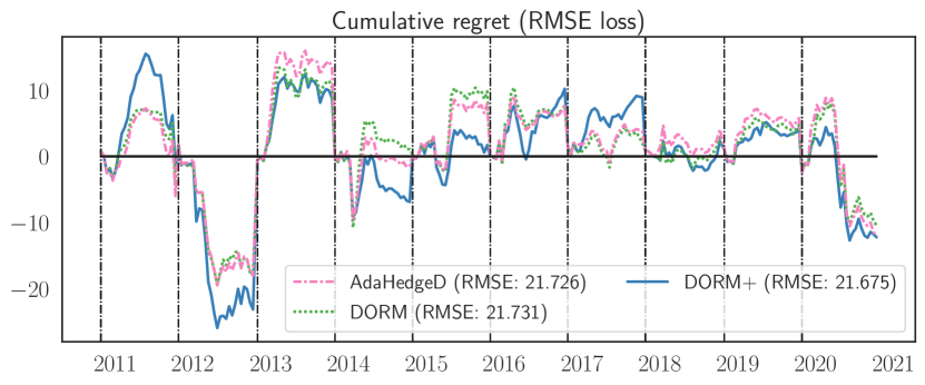
Precipitation Weeks 3-4

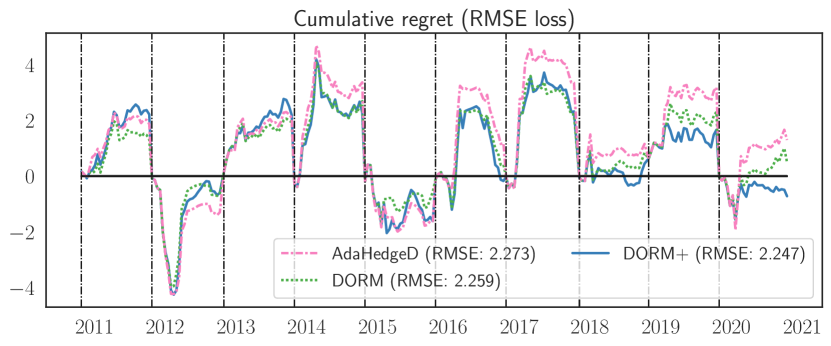
Temperature Weeks 3-4

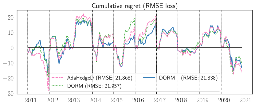
Precipitation Weeks 5-6

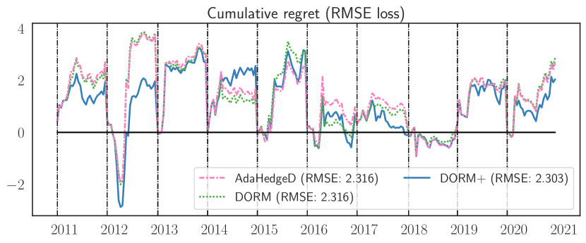
Temperature Weeks 5-6

Figure 6: Hint recent_g: Yearly cumulative regret under RMSE loss for the three delayed online learning algorithms presented, over the $10$-year evaluation period. The zero line corresponds to the performance of the best input model in a given year.

Table 3: Hint prev_g: Average RMSE of the 2010-2020 semimonthly forecasts for all four tasks over over a $10$-year evaluation period.

prev_g	AdaHedgeD	DORM	DORM+	Model1	Model2	Model3	Model4	Model5	Model6
Precip. 3-4w	21.760	21.777	21.729	21.973	22.431	22.357	21.978	21.986	23.344
Precip. 5-6w	21.943	21.964	21.911	22.030	22.570	22.383	22.004	21.993	23.257
Temp. 3-4w	2.266	2.269	2.250	2.253	2.352	2.394	2.277	2.319	2.508
Temp. 5-6w	2.306	2.307	2.305	2.270	2.368	2.459	2.278	2.317	2.569

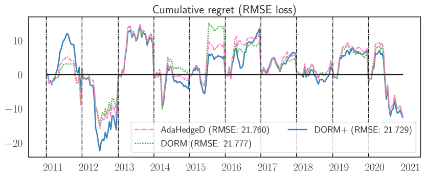
Precipitation Weeks 3-4

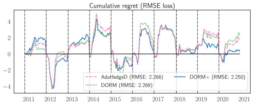
Temperature Weeks 3-4

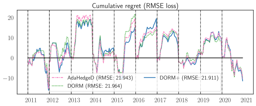
Precipitation Weeks 5-6

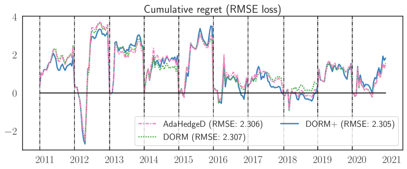
Temperature Weeks 5-6

Figure 7: Hint prev_g: Yearly cumulative regret under RMSE loss for the three delayed online learning algorithms presented.

Table 4: Hint mean_g: Average RMSE of the 2010-2020 semimonthly forecasts for all four tasks over over a $10$-year evaluation period.

mean_g	AdaHedgeD	DORM	DORM+	Model1	Model2	Model3	Model4	Model5	Model6
Precip. 3-4w	21.864	21.945	21.830	21.973	22.431	22.357	21.978	21.986	23.344
Precip. 5-6w	21.993	22.054	21.946	22.030	22.570	22.383	22.004	21.993	23.257
Temp. 3-4w	2.273	2.277	2.257	2.253	2.352	2.394	2.277	2.319	2.508
Temp. 5-6w	2.311	2.320	2.314	2.270	2.368	2.459	2.278	2.317	2.569

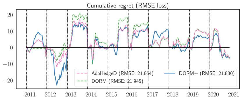
Precipitation Weeks 3-4

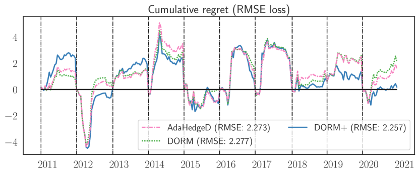
Temperature Weeks 3-4

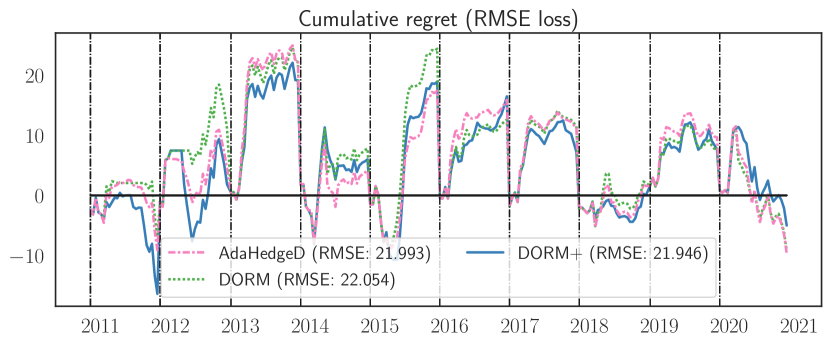
Precipitation Weeks 5-6

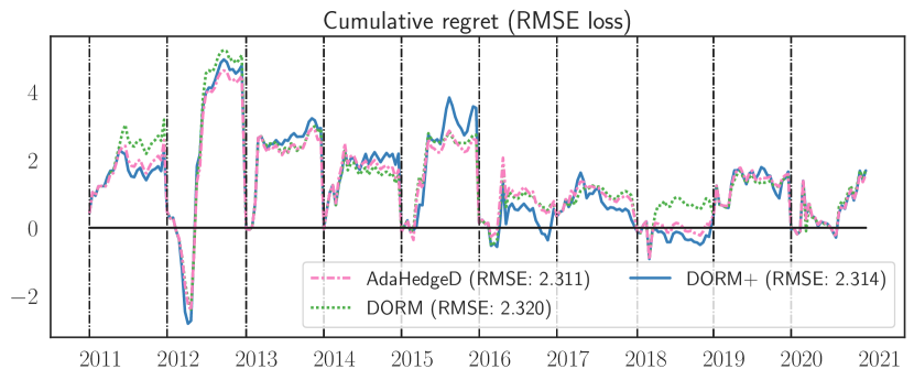
Temperature Weeks 5-6

Figure 8: Hint mean_g: Yearly cumulative regret under RMSE loss for the three delayed online learning algorithms presented.

Table 5: Hint none: Average RMSE of the 2010-2020 semimonthly forecasts for all four tasks over over a $10$-year evaluation period.

None	AdaHedgeD	DORM	DORM+	Model1	Model2	Model3	Model4	Model5	Model6
Precip. 3-4w	21.760	21.835	21.796	21.973	22.431	22.357	21.978	21.986	23.344
Precip. 5-6w	21.860	21.967	21.916	22.030	22.570	22.383	22.004	21.993	23.257
Temp. 3-4w	2.266	2.272	2.258	2.253	2.352	2.394	2.277	2.319	2.508
Temp. 5-6w	2.296	2.311	2.308	2.270	2.368	2.459	2.278	2.317	2.569

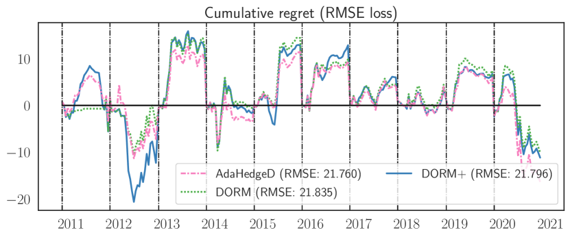
Precipitation Weeks 3-4

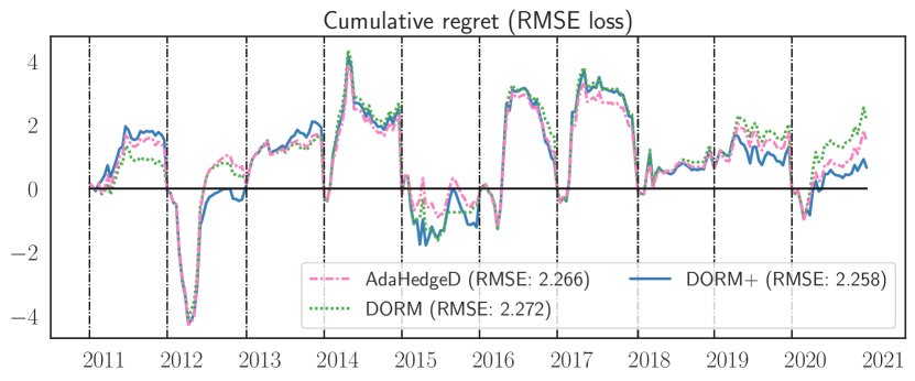
Temperature Weeks 3-4

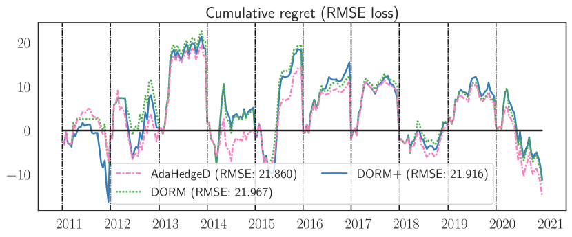
Precipitation Weeks 5-6

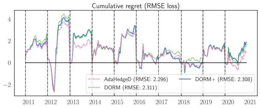
Temperature Weeks 5-6

Figure 9: Hint none: Yearly cumulative regret under RMSE loss for the three delayed online learning algorithms presented.

M.2 Impact of Regularization

Results for three regularization strategies—AdaHedgeD, DORM+, and DUB—on all four subseasonal prediction as described in Sec. 7. Fig. 10 shows the annual regret versus the best input model in any given year for each algorithm and task, and Fig. 11 presents an example of the weights played by each algorithm in the final evaluation year, as well as the regularization weight used by each algorithm.

The under- and over-regularization of AdaHedgeD and DUB respectively compared with DORM+ is evident in all four tasks, both in the regret and weight plots. Due to the looseness of the regularization settings used in DUB, its plays can be seen to be very close to the uniform ensemble in all four tasks. For this subseasonal prediction problem, the uniform ensemble is competitive, especially for the 5-6 week horizons. However, in problems where the uniform ensemble has higher regret, this over-regularization property of DUB would be undesirable. The more adaptive plays of DORM+ and AdaHedgeD have the potential to better exploit heterogeneous performance among different input models.

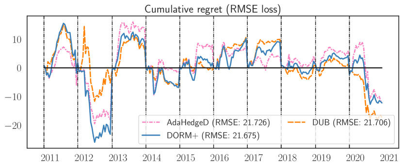
Precipitation Weeks 3-4

Temperature Weeks 3-4

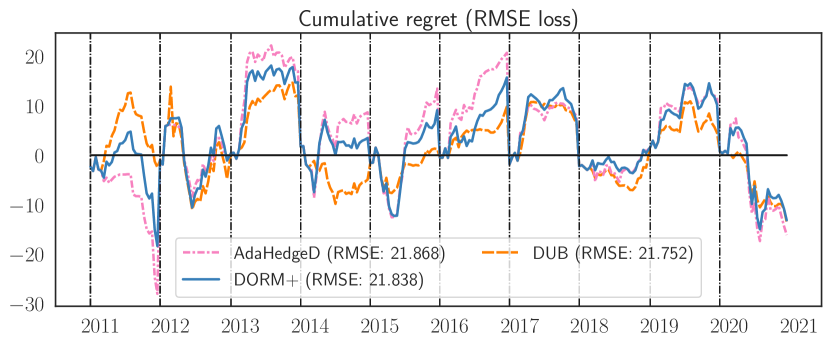
Precipitation Weeks 5-6

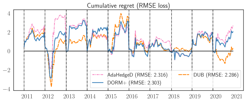
Temperature Weeks 5-6

Figure 10: Overall regret: Yearly cumulative regret under the RMSE loss for the three regularization algorithms presented.

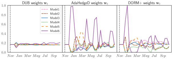
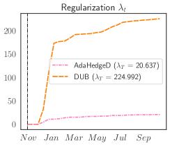
(a) Precipitation Weeks 3-4

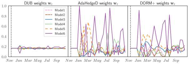
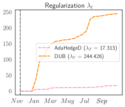
(b) Precipitation Weeks 5-6

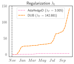
(c) Temperature Weeks 3-4

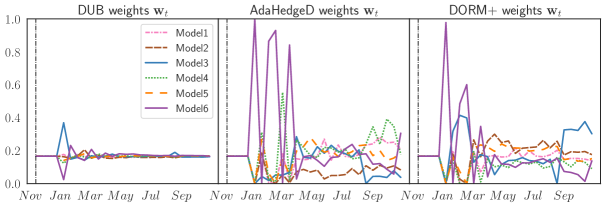
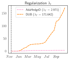
(d) Temperature Weeks 5-6

Figure 11: Impact of regularization: The plays $\mathbf{w}_{t}$ of online learning algorithms used to combine the input models for all four tasks in the 2020 evaluation year. The weights of DUB and AdaHedgeD appear respectively over and under regularized compared to DORM+ due to their selection of regularization strength $\lambda_{t}$ (right).

M.3 To Replicate or Not to Replicate

We compare the performance of replicated and non-replicated variants of our DORM+ algorithm as in Sec. 7. Both algorithms perform well, but in all tasks, DORM+ outperforms replicated DORM+ (in which $D+1$ independent copies of DORM+ make staggered predictions). Fig. 12 provides an example of the weight plots produced by the replication strategy for all for tasks.

The replicated algorithms only have the opportunity to learn from $T/(D+1)$ plays. For the 3-4 week horizons tasks $D=2$ and for the 5-6 week horizons tasks $D=3$. Because our forecasting horizons are short ($T=26$), further limiting the feedback available to each online learner via replication could be detrimental to practical model performance.

Table 6: Replication RMSE: Average RMSE of the 2010-2020 semimonthly forecasts for four tasks over over a $10$-year evaluation period for replicated versus standard DORM+.

	DORM+	Replicated DORM+	Model1	Model2	Model3	Model4	Model5	Model6
Precip. 3-4w	21.675	21.720	21.973	22.431	22.357	21.978	21.986	23.344
Precip. 5-6w	21.838	21.851	22.030	22.570	22.383	22.004	21.993	23.257
Temp. 3-4w	2.247	2.249	2.253	2.352	2.394	2.277	2.319	2.508
Temp. 5-6w	2.303	2.315	2.270	2.368	2.459	2.278	2.317	2.569

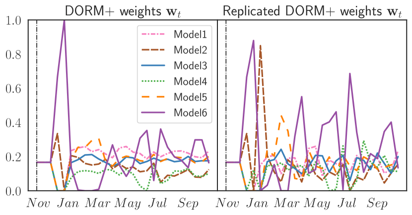
Precipitation Weeks 3-4

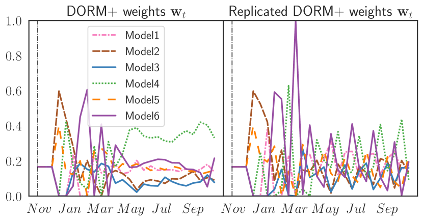
Temperature Weeks 3-4

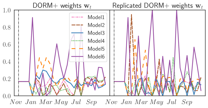
Precipitation Weeks 5-6

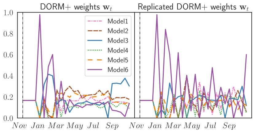
Temperature Weeks 5-6

Figure 12: Replication weights: The plays $\mathbf{w}_{t}$ of DORM+ and replicated DORM+ for all four tasks in the final evaluation year.

M.4 Learning to Hint

We examine the effect of optimism on the DORM+ algorithms and the ability of our “learning to hint” strategy to recover the performance of the best optimism strategy in retrospect as described in Sec. 7. We use DORM+ as the meta-algorithm for hint learning to produce the learned optimism strategy that plays a convex combination of the three constant hinters.

As reported in the main text, the regret of the base algorithm using the learned hinting strategy generally falls between the worst and the best hinting strategy for any given year. Because the best hinting strategy for any given year is unknown a priori, the adaptivity of the hint learner is useful practically. Currently, the hint learner is only optimizing a loose upper bound on base problem regret. Deriving loss functions for hint learning that more accurately quantify the effect of the hinter on base model regret is an important next step in achieving negative regret for online hinting algorithms.

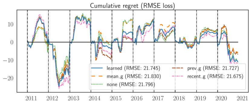
Precipitation Weeks 3-4

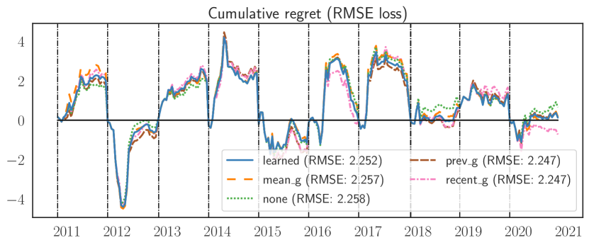
Temperature Weeks 3-4

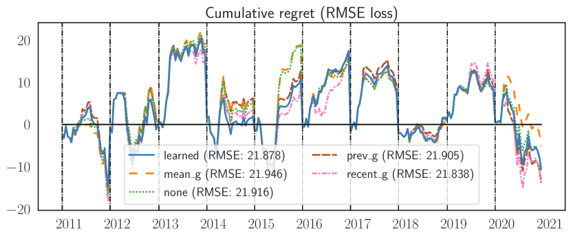
Precipitation Weeks 5-6

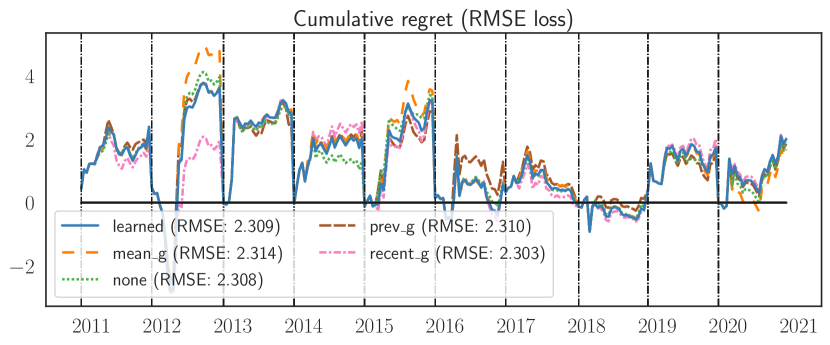
Temperature Weeks 5-6

Figure 13: Overall regret: Yearly cumulative regret under the RMSE loss for DORM+ using the three constant hinting strategies presented and the learned hinter, over the $10$-year evaluation period.

M.5 Impact of Different Forms of Optimism

The regret analysis presented in this work suggest that optimistic strategies under delay can benefit from hinting at both the “past” $\mathbf{g}_{t-D:t-1}$ missing losses and the “future” unobserved loss $\mathbf{g}_{t}$. To study the impact of different forms of optimism on DORM+, we provide a recent_g hint for either only the missing future loss $\mathbf{g}_{t}$, only the missing past losses $\mathbf{g}_{t-D:t-1}$, or both past and future losses (the strategy used in this paper) $\mathbf{g}_{t-D:t}$. Inspired by the recommendation of an anonymous reviewer, we also test two hint settings that only hint at the future unobserved loss but multiply the weight of that hint by 2D+1 or 3D+1, effectively increasing the importance of the future hint in the online learning optimization. Fig. 14 presents the experimental results.

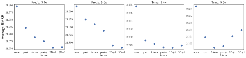
Figure 14: DORM+ average RMSE as in Table 1 as a function of optimism strategy; see Sec. M.5 for details.

In this experiment, all settings of optimism improve upon the non-optimistic algorithm, and, for all tasks, providing hints for missing future losses outperforms hinting at missing past losses. For all tasks save Temp. 5-6w, hinting at both missing past and future losses yields a further improvement. The 2D+1 and 3D+1 settings demonstrate that, for some tasks, increasing the magnitude of the optimistic hint can further improve performance in line with the online gradient descent predictions of Hsieh et al. (2020, Thm. 13).

Appendix N Algorithmic Details

N.1 ODAFTRL with AdaHedgeD and DUB tuning

The AdaHedgeD and DUB algorithms presented in the experiments are implementations of ODAFTRL with a negative entropy regularizer $\psi(\mathbf{w})=\sum_{j=1}^{d}\mathbf{w}_{j}\ln\mathbf{w}_{j}+\ln d$, which is $1$-strongly convex with respect to the norm $\|{\cdot}\|_{1}$ (Shalev-Shwartz, 2007, Lemma 16) with dual norm $\|{\cdot}\|_{\infty}$. Each algorithm optimizes over the simplex and competes with the simplex: $\mathbf{W}=\mathbf{U}=\triangle_{d-1}$. We choose $\alpha=\sup_{\mathbf{u}\in\mathbf{U}}\psi(\mathbf{u})=\ln(d)$. In the following, define $\psi_{t}\triangleq\lambda_{t}\psi$ for $\lambda_{t}\geq 0$. Our derivations of the update equations for AdaHedgeD and DUB make use of the following properties of the negative entropy regularizer, proved in Sec. N.4.

Lemma 28 (Negative entropy properties).

The negative entropy regularizer $\psi(\mathbf{w})=\sum_{j=1}^{d}\mathbf{w}_{j}\ln\mathbf{w}_{j}+\ln d$ with $\psi_{t}=\lambda_{t}\psi$ for $\lambda_{t}\geq 0$ satisfies the following properties on the simplex $\mathbf{W}=\triangle_{d-1}$.

$$\textstyle\psi_{\mathbf{W}}^{*}(\theta) \textstyle\triangleq\sup_{\mathbf{w}\in\mathbf{W}}\langle{\mathbf{w}},{\theta}\rangle-\psi(\mathbf{w})=\ln\Big{(}\sum_{j=1}^{d}\exp(\theta_{j})\Big{)}-\ln d,$$ (182)

$$\textstyle(\lambda\psi)_{\mathbf{W}}^{*}(\theta) \textstyle\triangleq\sup_{\mathbf{w}\in\mathbf{W}}\langle{\mathbf{w}},{\theta}\rangle-\lambda\psi(\mathbf{w})=\begin{cases}\lambda\psi_{\mathbf{W}}^{*}(\theta/\lambda)=\lambda\ln(\sum_{j=1}^{d}\exp(\theta_{j}/\lambda))-\lambda\ln d,&\text{if }\lambda>0\\ \max_{j\in[d]}\theta_{j}&\text{if }\lambda=0\end{cases},$$ (183)

$$\textstyle\mathbf{w}^{*}(\theta,\lambda) \textstyle\triangleq\begin{cases}\frac{\exp(\theta/\lambda)}{\sum_{j=1}^{d}\exp(\theta_{j}/\lambda)}&\text{if }\lambda>0\\ \frac{\mathbb{I}\mathopen{}\mathclose{{}\left[{\theta=\max_{j}\theta_{j}}}\right]}{\sum_{k\in[d]}\mathbb{I}\mathopen{}\mathclose{{}\left[{\theta_{k}=\max_{j}\theta_{j}}}\right]}&\text{if }\lambda=0\end{cases}\in\mathop{\mathrm{missing}}{argmin}_{\mathbf{w}\in\mathbf{W}}\lambda\psi(\mathbf{w})-\langle{\mathbf{w}},{\theta}\rangle\subseteq\partial(\lambda\psi)_{\mathbf{W}}^{*}(\theta).$$ (184)

Our next corollary concerning optimal ODAFTRL objectives follows directly from Lem. 28.

Corollary 29 (Optimal ODAFTRL objectives).

Instantiate the notation of Lem. 28, and define the functions $F_{t}(\mathbf{w},\lambda)\triangleq\lambda\psi(\mathbf{w})+\langle{\mathbf{g}_{1:t-1}},{\mathbf{w}}\rangle$ for $\mathbf{w}\in\mathbf{W}$. Then

$$\textstyle-(\lambda\psi)_{\mathbf{W}}^{*}(-(\mathbf{g}_{1:t-1}+\mathbf{h})) \textstyle=\inf_{\mathbf{w}\in\mathbf{W}}F_{t}(\mathbf{w},\lambda)+\langle{\mathbf{h}},{\mathbf{w}}\rangle\quad\text{and}\quad$$ (185)

$$\textstyle\mathbf{w}^{*}(-(\mathbf{g}_{1:t-1}+\mathbf{h}),\lambda) \textstyle=\mathop{\mathrm{missing}}{argmin}_{\mathbf{w}\in\mathbf{W}}F_{t}(\mathbf{w},\lambda)+\langle{\mathbf{h}},{\mathbf{w}}\rangle.$$ (186)

Using Lems. 28 and 29, we can derive an expression, proved in Sec. N.5, for the AdaHedgeD $\delta_{t}$ updates.

Proposition 30 (AdaHedgeD $\delta_{t}$).

Instantiate the notation of Thm. 12, and define the auxiliary hint vector

$$\textstyle\hat{\mathbf{h}}_{t}\triangleq\mathbf{g}_{t-D:t}+\sigma_{t}(\mathbf{h}_{t}-\mathbf{g}_{t-D:t})\quad\text{for}\quad\sigma_{t}\triangleq\min(\frac{\|{\mathbf{g}_{t}}\|_{*}}{\|{\mathbf{h}_{t}-\mathbf{g}_{t-D:t}}\|_{*}},1)$$ (187)

along with the scalars

$$\textstyle c_{*}=\max_{j:\mathbf{w}_{t,j}\neq 0}\mathbf{h}_{t,j}-\mathbf{g}_{t-D:t,j}\quad\text{and}\quad\hat{c}_{*}=\max_{j:\hat{\mathbf{w}}_{t,j}\neq 0}\hat{\mathbf{h}}_{t,j}-\mathbf{g}_{t-D:t,j}$$ (188)

for

$$\textstyle\bar{\mathbf{w}}_{t} \textstyle=\mathop{\mathrm{missing}}{argmin}_{\mathbf{w}\in\mathbf{W}}F_{t+1}(\mathbf{w},\lambda_{t})=\frac{\exp(-\mathbf{g}_{1:t}/\lambda_{t})}{\sum_{j=1}^{d}\exp(-\mathbf{g}_{1:t,j}/\lambda_{t})}\quad\text{and}\quad$$ (189)

$$\textstyle\hat{\mathbf{w}}_{t} \textstyle=\mathop{\mathrm{missing}}{argmin}_{\mathbf{w}\in\mathbf{W}}F_{t+1}(\mathbf{w},\lambda_{t})+\langle{\hat{\mathbf{h}}_{t}-\mathbf{g}_{t-D:t}},{\mathbf{w}}\rangle=\frac{\exp(-(\mathbf{g}_{1:t-D-1}+\hat{\mathbf{h}}_{t})/\lambda_{t})}{\sum_{j=1}^{d}\exp(-(\mathbf{g}_{1:t-D-1,j}+\hat{\mathbf{h}}_{t,j})/\lambda_{t})}$$ (190)

by Cor. 29. If $\lambda_{t}>0$,

$$\textstyle\delta_{t} \textstyle=\min(\delta_{t}^{(1)},\delta_{t}^{(2)},\delta_{t}^{(3)})_{+}\quad\text{for}\quad$$ (191)

$$\textstyle\delta_{t}^{(1)} \textstyle=F_{t+1}(\mathbf{w}_{t},\lambda_{t})-F_{t+1}(\bar{\mathbf{w}}_{t},\lambda_{t})$$ (192)

$$\textstyle=\lambda_{t}\ln(\sum_{j\in[d]}\mathbf{w}_{t,j}\exp((\mathbf{h}_{t,j}-\mathbf{g}_{t-D:t,j})/\lambda_{t}))+\langle{\mathbf{g}_{t-D:t}-\mathbf{h}_{t}},{\mathbf{w}_{t}}\rangle$$ (193)

$$\textstyle=\lambda_{t}\ln(\sum_{j\in[d]}\mathbf{w}_{t,j}\exp((\mathbf{h}_{t,j}-\mathbf{g}_{t-D:t,j}-c_{*})/\lambda_{t}))+\langle{\mathbf{g}_{t-D:t}-\mathbf{h}_{t}},{\mathbf{w}_{t}}\rangle+c_{*},$$ (194)

$$\textstyle\delta_{t}^{(2)} \textstyle=\langle{\mathbf{g}_{t}},{\mathbf{w}_{t}-\bar{\mathbf{w}}_{t}}\rangle,\quad\text{and}\quad$$ (195)

$$\textstyle\delta_{t}^{(3)} \textstyle=F_{t+1}(\hat{\mathbf{w}}_{t},\lambda_{t})-F_{t+1}(\bar{\mathbf{w}}_{t},\lambda_{t})+\langle{\mathbf{g}_{t}},{\mathbf{w}_{t}-\hat{\mathbf{w}}_{t}}\rangle$$ (196)

$$\textstyle=\lambda_{t}\ln(\sum_{j\in[d]}\hat{\mathbf{w}}_{t,j}\exp((\hat{\mathbf{h}}_{t,j}-\mathbf{g}_{t-D:t,j})/\lambda_{t}))+\langle{\mathbf{g}_{t-D:t}-\hat{\mathbf{h}}_{t}},{\hat{\mathbf{w}}_{t}}\rangle+\langle{\mathbf{g}_{t}},{\mathbf{w}_{t}-\hat{\mathbf{w}}_{t}}\rangle$$ (197)

$$\textstyle=\lambda_{t}\ln(\sum_{j\in[d]}\hat{\mathbf{w}}_{t,j}\exp((\hat{\mathbf{h}}_{t,j}-\mathbf{g}_{t-D:t,j}-\hat{c}_{*})/\lambda_{t}))+\langle{\mathbf{g}_{t-D:t}-\hat{\mathbf{h}}_{t}},{\hat{\mathbf{w}}_{t}}\rangle+\hat{c}_{*}+\langle{\mathbf{g}_{t}},{\mathbf{w}_{t}-\hat{\mathbf{w}}_{t}}\rangle.$$ (198)

If $\lambda_{t}=0$,

$$\textstyle\delta_{t} \textstyle=\min(\delta_{t}^{(1)},\delta_{t}^{(2)},\delta_{t}^{(3)})_{+}\quad\text{for}\quad$$ (199)

$$\textstyle\delta_{t}^{(1)} \textstyle=\langle{\mathbf{g}_{1:t}},{\mathbf{w}_{t}}\rangle-\min_{j\in[d]}\mathbf{g}_{1:t,j},$$ (200)

$$\textstyle\delta_{t}^{(2)} \textstyle=\langle{\mathbf{g}_{t}},{\mathbf{w}_{t}-\bar{\mathbf{w}}_{t}}\rangle,\quad\text{and}\quad$$ (201)

$$\textstyle\delta_{t}^{(3)} \textstyle=\langle{\mathbf{g}_{1:t}},{\hat{\mathbf{w}}_{t}}\rangle-\min_{j\in[d]}\mathbf{g}_{1:t,j}+\langle{\mathbf{g}_{t}},{\mathbf{w}_{t}-\hat{\mathbf{w}}_{t}}\rangle.$$ (202)

Leveraging these results, we present the pseudocode for the AdaHedgeD and DUB instantiations of ODAFTRL in Algorithm 1.

Algorithm 1 ODAFTRL with $\mathbf{W}=\triangle_{d-1}$, $\psi(\mathbf{w})=\sum_{j=1}^{d}\mathbf{w}_{j}\ln\mathbf{w}_{j}+\ln(d)$, delay $D\geq 0$, and tuning strategy tuning

1:  Parameter $\alpha=\sup_{\mathbf{u}\in\triangle_{d-1}}\psi(\mathbf{u})=\ln(d)$

2:  Initial regularization weight: $\lambda_{0}=0$

3:  if tuning is DUB then

4:     Initial regularization sum: $\Delta_{0}=0$

5:     Initial maximum: $\mathbf{a}^{\max}=0$

6:  end if

7:  Initial subgradient sum: $\mathbf{g}_{1:1}=\mathbf{0}\in\mathbb{R}^{d}$

8:  Dummy losses and iterates: $\mathbf{g}_{-D}=\cdots=\mathbf{g}_{0}=\mathbf{0}\in\mathbb{R}^{d}$, $\mathbf{w}_{-D}=\cdots=\mathbf{w}_{0}=\mathbf{0}\in\mathbb{R}^{d}$

9:  for $t=1,\dots,T$ do

10:     Receive hint $\mathbf{h}_{t}\in\mathbb{R}^{d}$

11:     Output $\mathbf{w}_{t}=\mathop{\mathrm{missing}}{argmin}_{\mathbf{w}\in\mathbf{W}}F_{t-D}(\mathbf{w},\lambda_{t})+\langle{\mathbf{h}_{t}},{\mathbf{w}}\rangle$ as in Cor. 29

12:     Receive $\mathbf{g}_{t-D}\in\mathbb{R}^{d}$ and pay $\langle\mathbf{g}_{t-D},\mathbf{w}_{t-D}\rangle$

13:     Update subgradient sum $\mathbf{g}_{1:t-D}=\mathbf{g}_{1:t-D-1}+\mathbf{g}_{t-D}$

14:     if tuning is AdaHedgeD then

15:        Compute the auxiliary play $\bar{\mathbf{w}}_{t-D}=\mathop{\mathrm{missing}}{argmin}_{\mathbf{w}\in\mathbf{W}}F_{t-D+1}(\mathbf{w},\lambda_{t-D})$ as in Cor. 29

16:        Compute the auxiliary regret term $\delta_{t-D}^{(1)}=F_{t-D+1}(\mathbf{w}_{t-D},\lambda_{t-D})-F_{t-D+1}(\bar{\mathbf{w}}_{t-D},\lambda_{t-D})$ as in Prop. 30

17:        Compute the drift term $\delta_{t-D}^{(2)}=\langle{\mathbf{g}_{t-D}},{\mathbf{w}_{t-D}-\bar{\mathbf{w}}_{t-D}}\rangle$

18:        Compute the auxiliary hint 187 $\hat{\mathbf{h}}_{t-D}\triangleq\mathbf{g}_{t-2D:t-D}+\min(\frac{\|{\mathbf{g}_{t-D}}\|_{*}}{\|{\mathbf{h}_{t-D}-\mathbf{g}_{t-2D:t-D}}\|_{*}},1)(\mathbf{h}_{t-D}-\mathbf{g}_{t-2D:t-D})$

19:        Compute the auxiliary play $\hat{\mathbf{w}}_{t-D}=\mathop{\mathrm{missing}}{argmin}_{\mathbf{w}\in\mathbf{W}}F_{t-D+1}(\mathbf{w},\lambda_{t-D})+\langle{\hat{\mathbf{h}}_{t-D}-\mathbf{g}_{t-2D:t-D}},{\mathbf{w}}\rangle$ as in Cor. 29

20:        Compute the regret term $\delta_{t-D}^{(3)}=F_{t-D+1}(\hat{\mathbf{w}}_{t-D},\lambda_{t-D})-F_{t-D+1}(\bar{\mathbf{w}}_{t-D},\lambda_{t-D})+\langle{\mathbf{g}_{t-D}},{\mathbf{w}_{t-D}-\hat{\mathbf{w}}_{t-D}}\rangle$ as in Prop. 30

21:        Update $\lambda_{t+1}=\lambda_{t}+\frac{1}{\alpha}\min(\delta_{t-D}^{(1)},\delta_{t-D}^{(2)},\delta_{t-D}^{(3)})_{+}$ as in 28

22:     else if tuning is DUB then

23:        Compute $\mathbf{a}_{t-D,F}=2\min\big{(}\|{\mathbf{g}_{t-D}}\|_{\infty},\|{\mathbf{h}_{t-D}-\sum_{s=t-2D}^{t-D}\mathbf{g}_{s}}\|_{\infty}\big{)}$ as in 21

24:        Compute $\mathbf{b}_{t-D,F}=\frac{1}{2}\|{\mathbf{h}_{t-D}-\sum_{s=t-2D}^{t-D}\mathbf{g}_{s}}\|_{\infty}^{2}-\frac{1}{2}(\|{\mathbf{h}_{t-D}-\sum_{s=t-2D}^{t-D}\mathbf{g}_{s}}\|_{\infty}-\|{\mathbf{g}_{t-D}}\|_{\infty})_{+}^{2}$ as in 21

25:        Update $\Delta_{t+1}=\Delta_{t}+\mathbf{a}_{t-D,F}^{2}+2\alpha\mathbf{b}_{t-D,F}$

26:        Update maximum $\mathbf{a}^{\max}=\max(\mathbf{a}^{\max},\mathbf{a}_{t-2D:t-D-1,F})$

27:        Update $\lambda_{t+1}=\frac{1}{\alpha}(2\mathbf{a}^{\max}+\sqrt{\Delta_{t+1}})$ as in DUB

28:     end if

29:  end for

N.2 DORM and DORM+

The DORM and DORM+ algorithms presented in the experiments are implementations of ODAFTRL and DOOMD respectively that play iterates in $\mathbf{W}\triangleq\triangle_{d-1}$ using the default value $\lambda=1$. Both algorithms use a $p$-norm regularizer $\psi=\frac{1}{2}\|{\cdot}\|_{p}^{2}$, which is $1$-strongly convex with respect to $\|{\cdot}\|=\sqrt{p-1}\|{\cdot}\|_{p}$ (see Shalev-Shwartz, 2007, Lemma 17) with $\|{\cdot}\|_{*}=\frac{1}{\sqrt{p-1}}\|{\cdot}\|_{q}$. For the paper experiments, we choose the optimal value $q=\inf_{q^{\prime}\geq 2}d^{2/q^{\prime}}(q^{\prime}-1)$ to obtain $\ln(d)$ scaling in the algorithm regret; for $d=6$, $p=q=2$. The update equations for each algorithm are given in the main text by DORM and DORM+ respectively. The optimistic hinters provide delayed gradient hints $\tilde{\mathbf{g}}_{t}$, which are then used to compute regret gradient hints $\tilde{\mathbf{r}}_{t}$, where $\tilde{\mathbf{r}}_{t}=\langle{\tilde{\mathbf{g}}_{t}},{\mathbf{w}_{t}}\rangle-\tilde{\mathbf{g}}_{t}$ and $\mathbf{h}_{t}=\sum_{s=t-D}^{t-1}\tilde{\mathbf{r}}_{s}+\langle{\tilde{\mathbf{g}}_{t}},{\mathbf{w}_{t-1}}\rangle-\tilde{\mathbf{g}}_{t}$.

N.3 Adaptive Hinting

For the adaptive hinting experiments, we use the DORM+ as both the base and hint learner. For the hint learner with DORM base algorithm, the hint loss function is given by 169 with $q=2$. The plays of the online hinter $\omega_{t}$ are used to generate the hints $\mathbf{h}_{t}$ for the base algorithm using the hint matrix $H_{t}\in\mathbb{R}^{d\times m}$. The $j$-th column of $H_{t}$ contains hinter $j$’s predictions for the cumulative missing regret subgradients $\mathbf{r}_{t-D:t}$. The final hint for the base learner is $\mathbf{h}_{t}=H_{t}\omega_{t}$. Psuedo-code for the adaptive hinter is given in Algorithm 2.

Algorithm 2 Learning to hint with DORM+ ($q$=2) hint learner, DORM+ base learner, and delay $D\geq 0$

1:  Subgradient vector: $\mathbf{g}_{-D},\cdots\mathbf{g}_{0}=\mathbf{0}\in\mathbb{R}^{d}$

2:  Meta-subgradient vector: $\gamma_{-D},\cdots\gamma_{0}=\mathbf{0}\in\mathbb{R}^{m}$

3:  Initial instantaneous regret: $\mathbf{r}_{-D}=\mathbf{0}\in\mathbb{R}^{d}$

4:  Initial instantaneous meta-regret: $\rho_{-D}=\mathbf{0}\in\mathbb{R}^{m}$

5:  Initial hint $\mathbf{h}_{0}=\mathbf{0}\in\mathbb{R}^{d}$

6:  Initial orthant meta-vector: $\tilde{\omega}_{0}=\mathbf{0}\in\mathbb{R}^{m}$

7:  for $t=1,\dots,T$ do

8:     // Update online hinter using DORM+ with $q=2$

9:     Find optimal unnormalized hint combination vector $\tilde{\omega}_{t}=\max(\mathbf{0},\tilde{\omega}_{t-1}+\rho_{t-D-1})$

10:     Normalize: $\omega_{t}=\begin{cases}\mathbf{1}/m&\text{if }\tilde{\omega}_{t}=\mathbf{0}\\ \tilde{\omega}_{t}/\langle{\mathbf{1}},{\tilde{\omega}_{t}}\rangle&\text{otherwise}\end{cases}$

11:     Receive hint matrix: $H_{t}\in\mathbb{R}^{d\times m}$ in which each column is a hint for $\sum_{s=t-D}^{t}\mathbf{r}_{s}$

12:     Output hint $\mathbf{h}_{t}=H_{t}\omega_{t}$

13:     // Update DORM+ base learner and get next play

14:     Output $\mathbf{w}_{t}=\lx@cref{creftype~refnum}{dorm+}(\mathbf{g}_{t-D-1},\mathbf{h}_{t})$

15:     Receive $\mathbf{g}_{t-D}\in\mathbb{R}^{d}$ and pay $\langle\mathbf{g}_{t-D},\mathbf{w}_{t-D}\rangle$

16:     Compute instantaneous regret $\mathbf{r}_{t-D}=\mathbf{1}\langle{\mathbf{g}_{t-D}},{\mathbf{w}_{t-D}}\rangle-\mathbf{g}_{t-D}$

17:     Compute hint meta-subgradient $\gamma_{t-D}\in\partial l_{t-D}(\omega_{t-D})\in\mathbb{R}^{m}$ as in 171

18:     Compute instantaneous hint regret $\rho_{t-D}=\mathbf{1}\langle{\gamma_{t-D}},{\omega_{t-D}}\rangle-\gamma_{t-D}$

19:  end for

N.4 Proof of Lem. 28: Negative entropy properties

The expression of the Fenchel conjugate for $\lambda>0$ is derived by solving an appropriate constrained convex optimization problem for $\mathbf{w}=\triangle_{d-1}$, as shown in Orabona (2019, Section 6.6). The value of $\mathbf{w}^{*}(\theta,\lambda)\in\partial(\lambda\psi)_{\mathbf{W}}^{*}(\theta)$ uses the properties of the Fenchel conjugate (Rockafellar, 1970; Orabona, 2019, Theorem 5.5) and is shown in Orabona (2019, Theorem 6.6).

N.5 Proof of Prop. 30: AdaHedgeD $\delta_{t}$

First suppose $\lambda_{t}>0$. The first term in the $\min$ of AdaHedgeD’s $\delta_{t}$ setting is derived as follows:

$$\textstyle\delta_{t}^{(1)} \textstyle\triangleq F_{t+1}(\mathbf{w}_{t},\lambda_{t})-F_{t+1}(\bar{\mathbf{w}}_{t},\lambda_{t})\quad\text{by definition \lx@cref{creftype~refnum}{def-deltat}}\quad$$ (203)

$$\textstyle=F_{t-D}(\mathbf{w}_{t},\lambda_{t})+\langle{\mathbf{h}_{t}},{\mathbf{w}_{t}}\rangle+\langle{\mathbf{g}_{t-D:t}-\mathbf{h}_{t}},{\mathbf{w}_{t}}\rangle-\inf_{\mathbf{w}\in\mathbf{W}}F_{t+1}(\mathbf{w},\lambda_{t})\quad\text{by definition of $\bar{\mathbf{w}}_{t}$}\quad$$ (204)

$$\textstyle=F_{t-D}(\mathbf{w}_{t},\lambda_{t})+\langle{\mathbf{h}_{t}},{\mathbf{w}_{t}}\rangle+\langle{\mathbf{g}_{t-D:t}-\mathbf{h}_{t}},{\mathbf{w}_{t}}\rangle+\lambda_{t}\psi_{\mathbf{W}}^{*}(-\mathbf{g}_{1:t}/\lambda_{t})\quad\text{by \lx@cref{creftype~refnum}{ftrl-obj-def}}\quad$$ (205)

$$\textstyle=\lambda_{t}\psi_{\mathbf{W}}^{*}(-\mathbf{g}_{1:t}/\lambda_{t})-\lambda_{t}\psi_{\mathbf{W}}^{*}((-\mathbf{h}_{t}-\mathbf{g}_{1:t-D-1})/\lambda_{t})+\langle{\mathbf{g}_{t-D:t}-\mathbf{h}_{t}},{\mathbf{w}_{t}}\rangle$$ (206)

because $$\mathbf{w}_{t}\in\mathop{\mathrm{missing}}{argmin}_{\mathbf{w}\in\mathbf{W}}F_{t-D}(\mathbf{w}_{t},\lambda_{t})+\langle{\mathbf{h}_{t}},{\mathbf{w}_{t}}\rangle$$ (207)

$$\textstyle=\lambda_{t}(\ln(\sum_{j=1}^{d}\exp(-\mathbf{g}_{1:t,j}/\lambda_{t}))-\lambda_{t}(\ln(\sum_{j=1}^{d}\exp((-\mathbf{g}_{1:t-D-1,j}-\mathbf{h}_{t,j})/\lambda_{t}))+\langle{\mathbf{g}_{t-D:t}-\mathbf{h}_{t}},{\mathbf{w}_{t}}\rangle\quad\text{by \lx@cref{creftype~refnum}{entropy_properties}}\quad$$ (208)

$$\textstyle=\lambda_{t}\ln\mathopen{}\mathclose{{}\left(\sum_{j=1}^{d}\frac{\exp(-\mathbf{g}_{1:t,j}/\lambda_{t})}{\sum_{j=1}^{d}\exp((-\mathbf{g}_{1:t-D-1,j}-\mathbf{h}_{t,j})/\lambda_{t})}}\right)+\langle{\mathbf{g}_{t-D:t}-\mathbf{h}_{t}},{\mathbf{w}_{t}}\rangle$$ (209)

$$\textstyle=\lambda_{t}\ln\mathopen{}\mathclose{{}\left(\sum_{j=1}^{d}\frac{\exp((-\mathbf{g}_{1:t-D-1,j}-\mathbf{h}_{t,j})/\lambda_{t})\exp((\mathbf{h}_{t,j}-\mathbf{g}_{t-D:t,j})/\lambda_{t})}{\sum_{j=1}^{d}\exp((-\mathbf{g}_{1:t-D-1,j}-\mathbf{h}_{t,j})/\lambda_{t})}}\right)+\langle{\mathbf{g}_{t-D:t}-\mathbf{h}_{t}},{\mathbf{w}_{t}}\rangle$$ (210)

$$\textstyle=\lambda_{t}\ln\mathopen{}\mathclose{{}\left(\sum_{j=1}^{d}\mathbf{w}_{t,j}\exp((\mathbf{h}_{t,j}-\mathbf{g}_{t-D:t,j})/\lambda_{t})}\right)+\langle{\mathbf{g}_{t-D:t}-\mathbf{h}_{t}},{\mathbf{w}_{t}}\rangle\quad\text{by the expression for $\mathbf{w}_{t}$ in \lx@cref{creftype~refnum}{ftrl-obj-def}.}\quad$$ (211)

The expression for the third term in the $\min$ of AdaHedgeD’s $\delta_{t}$ setting follows from identical reasoning.

Now suppose $\lambda_{t}=0$. We have

$$\textstyle\delta_{t}^{(1)} \textstyle\triangleq F_{t+1}(\mathbf{w}_{t},\lambda_{t})-F_{t+1}(\bar{\mathbf{w}}_{t},\lambda_{t})\quad\text{by definition \lx@cref{creftype~refnum}{def-deltat}}\quad$$ (212)

$$\textstyle=\langle{\mathbf{g}_{1:t}},{\mathbf{w}_{t}}\rangle-\inf_{\mathbf{w}\in\mathbf{W}}F_{t+1}(\mathbf{w},\lambda_{t})\quad\text{by definition of $\bar{\mathbf{w}}_{t}$}\quad$$ (213)

$$\textstyle=\langle{\mathbf{g}_{1:t}},{\mathbf{w}_{t}}\rangle-\min_{j\in[d]}\mathbf{g}_{1:t,j}\quad\text{by \lx@cref{creftype~refnum}{ftrl-obj-def}.}\quad$$ (214)

Identical reasoning yields the advertised expression for the third term.

Appendix O Extension to Variable and Unbounded Delays

In this section we detail how our main results generalize to the case of variable and potentially unbounded delays. For each time $t$, we define $\textup{last}(t)$ as the largest index $s$ for which $\mathbf{g}_{1:s}$ is observable at time $t$ (that is, available for constructing $\mathbf{w}_{t}$) and $\textup{first}(t)$ as the first time $s$ at which $\mathbf{g}_{1:t}$ is observable at time $s$ (that is, available for constructing $\mathbf{w}_{s}$).

O.1 Regret of DOOMD with variable delays

Consider the DOOMD variable-delay generalization

$$\mathbf{w}_{t+1}=\mathop{\mathrm{missing}}{argmin}_{\mathbf{w}\in\mathbf{W}}\,\langle{\mathbf{g}_{\textup{last}(t)+1:\textup{last}(t+1)}+\mathbf{h}_{t+1}-\mathbf{h}_{t}},{\mathbf{w}}\rangle+\mathcal{B}_{\lambda\psi}(\mathbf{w},\mathbf{w}_{t})\quad\text{with}\quad\mathbf{h}_{0}\triangleq\mathbf{0}\quad\text{and arbitrary}\quad\mathbf{w}_{0}.$$ (DOOMD with variable delays)

We first note that DOOMD with variable delays is an instance of SOOMD respectively with a “bad” choice of optimistic hint $\tilde{\mathbf{g}}_{t+1}$ that deletes the unobserved loss subgradients $\mathbf{g}_{\textup{last}(t+1)+1:t}$.

Lemma 31 (DOOMD with variable delays is SOOMD with a bad hint).

DOOMD with variable delays is SOOMD with $\tilde{\mathbf{g}}_{t+1}=\tilde{\mathbf{g}}_{t}+\mathbf{g}_{\textup{last}(t)+1:\textup{last}(t+1)}-\mathbf{g}_{t}+\mathbf{h}_{t+1}-\mathbf{h}_{t}=\mathbf{h}_{t+1}+\sum_{s=1}^{t}\mathbf{g}_{\textup{last}(s)+1:\textup{last}(s+1)}-\mathbf{g}_{s}.=\mathbf{h}_{t+1}-\mathbf{g}_{\textup{last}(t+1)+1:t}.$

The following result now follows immediately from Thms. 4 and 31.

Theorem 32 (Regret of DOOMD with variable delays).

If $\psi$ is differentiable and $\mathbf{h}_{T+1}\triangleq\mathbf{g}_{\textup{last}(T+1)+1:T}$, then, for all $\mathbf{u}\in\mathbf{W}$, the DOOMD with variable delays iterates $\mathbf{w}_{t}$ satisfy

$$\textstyle\textup{Regret}_{T}(\mathbf{u}) \textstyle\leq\mathcal{B}_{\lambda\psi}(\mathbf{u},\mathbf{w}_{0})+\frac{1}{\lambda}\sum_{t=1}^{T}\mathbf{b}_{t,O}^{2},\quad\text{for}\quad$$ (215)

$$\textstyle\mathbf{b}_{t,O}^{2} \textstyle\triangleq\textup{huber}(\|{\mathbf{h}_{t}-\sum_{s=\textup{last}(t)+1}^{t}\mathbf{g}_{s}}\|_{*},\|{\mathbf{g}_{\textup{last}(t)+1:\textup{last}(t+1)}+\mathbf{h}_{t+1}-\mathbf{h}_{t}}\|_{*}).$$ (216)

O.2 Regret of ODAFTRL with variable delays

Consider the ODAFTRL variable-delay generalization

$$\mathbf{w}_{t+1}=\mathop{\mathrm{missing}}{argmin}_{\mathbf{w}\in\mathbf{W}}\,\langle{\mathbf{g}_{1:\textup{last}(t+1)}+\mathbf{h}_{t+1}},{\mathbf{w}}\rangle+\lambda_{t+1}\psi(\mathbf{w}).$$ (ODAFTRL with variable delays)

Since ODAFTRL with variable delays is an instance of OAFTRL with $\tilde{\mathbf{g}}_{t+1}=\mathbf{h}_{t+1}-\sum_{s=\textup{last}(t+1)+1}^{t}\mathbf{g}_{s}$, the following result follows immediately from the OAFTRL regret bound, Thm. 14.

Theorem 33 (Regret of ODAFTRL with variable delays).

If $\psi$ is nonnegative and $\lambda_{t}$ is non-decreasing in $t$, then, $\forall\mathbf{u}\in\mathbf{W}$, the ODAFTRL with variable delays iterates $\mathbf{w}_{t}$ satisfy

$$\textstyle\textup{Regret}_{T}(\mathbf{u}) \textstyle\leq\lambda_{T}\psi(\mathbf{u})+\sum_{t=1}^{T}\min(\frac{\mathbf{b}_{t,F}}{\lambda_{t}},\mathbf{a}_{t,F})\quad\text{with}\quad$$ (217)

$$\textstyle\mathbf{b}_{t,F} \textstyle\triangleq\textup{huber}(\|{\mathbf{h}_{t}-\sum_{s=\textup{last}(t)+1}^{t}\mathbf{g}_{s}}\|_{*},\|{\mathbf{g}_{t}}\|_{*})\quad\text{and}\quad$$ (218)

$$\textstyle\mathbf{a}_{t,F} \textstyle\triangleq\operatorname{diam}({\mathbf{W}})\min\big{(}\|{\mathbf{h}_{t}-\sum_{s=\textup{last}(t)+1}^{t}\mathbf{g}_{s}}\|,\|{\mathbf{g}_{t}}\|_{*}\big{)}.$$ (219)

O.3 Regret of DUB with variable delays

Consider the DUB variable-delay generalization

$$\alpha\lambda_{t+1}=2\max_{j\leq\textup{last}(t+1)-1}\mathbf{a}_{\textup{last}(j+1)+1:j,F}+\textstyle\sqrt{\sum_{i=1}^{\textup{last}(t+1)}\mathbf{a}_{i,F}^{2}+2\alpha\mathbf{b}_{i,F}}.$$ (DUB with variable delays)

Theorem 34 (Regret of DUB with variable delays).

Fix $\alpha>0$, and, for $\mathbf{a}_{t,F},\mathbf{b}_{t,F}$ as in 218, consider the DUB with variable delays sequence. If $\psi$ is nonnegative, then, for all $\mathbf{u}\in\mathbf{W}$, the ODAFTRL with variable delays iterates $\mathbf{w}_{t}$ satisfy

$$\textstyle\textup{Regret}_{T}(\mathbf{u})\leq\big{(}\frac{\psi(\mathbf{u})}{\alpha}+1\big{)}$$ (220)

$$\textstyle\big{(}2\max_{t\in[T]}\mathbf{a}_{\textup{last}(t)+1:t-1,F}+\textstyle\sqrt{\sum_{t=1}^{T}\mathbf{a}_{t,F}^{2}+2\alpha\mathbf{b}_{t,F}}\big{)}$$ (221)

Proof.

Fix any $\mathbf{u}\in\mathbf{W}$. By Thm. 33, ODAFTRL with variable delays admits the regret bound

$$\textstyle\textup{Regret}_{T}(\mathbf{u})\leq\lambda_{T}\psi(\mathbf{u})+\sum_{t=1}^{T}\min(\frac{1}{\lambda_{t}}\mathbf{b}_{t,F},\mathbf{a}_{t,F}).$$ (222)

To control the second term in this bound, we apply the following lemma proved in Sec. H.1.

Lemma 35 (DUB with variable delays-style tuning bound).

Fix any $\alpha>0$ and any non-negative sequences $(a_{t})_{t=1}^{T}$, $(b_{t})_{t=1}^{T}$. If $(\lambda_{t})_{t\geq 1}$ is non-decreasing and

$$\textstyle\Delta_{t+1}^{*}\triangleq 2\max_{j\leq\textup{last}(t+1)-1}a_{\textup{last}(j+1)+1:j}+\sqrt{\sum_{i=1}^{\textup{last}(t+1)}a_{i}^{2}+2\alpha b_{i}}\leq\alpha\lambda_{t+1}\quad\text{for each}\quad t$$ (223)

then

$$\textstyle\sum_{t=1}^{T}\min(b_{t}/\lambda_{t},a_{t})\leq\Delta_{\textup{first}(T)}^{*}\leq\alpha\lambda_{\textup{first}(T)}.$$ (224)

∎

Since $T\leq\textup{first}(T)$, $\lambda_{T}\leq\lambda_{\textup{first}(T)}$, and $\textup{last}(\textup{first}(T))=T$, the result now follows by setting $a_{t}=\mathbf{a}_{t,F}$ and $b_{t}=\mathbf{b}_{t,F}$, so that

$$\textstyle\textup{Regret}_{T}(\mathbf{u})\leq\lambda_{T}\psi(\mathbf{u})+\alpha\lambda_{\textup{first}(T)}\leq(\psi(\mathbf{u})+\alpha)\lambda_{\textup{first}(T)}.$$ (225)

O.4 Proof of Lem. 35: DUB with variable delays-style tuning bound

We prove the claim

$$\textstyle\Delta_{t}\triangleq\sum_{i=1}^{t}\min(b_{i}/\lambda_{i},a_{i})\leq\Delta_{\textup{first}(t)}^{*}\leq\alpha\lambda_{\textup{first}(t)}$$ (226)

by induction on $t$.

Base case

For $t=1$, since $\textup{last}(\textup{first}(t))\geq t$, we have

$$\textstyle\sum_{i=1}^{t}\min(b_{i}/\lambda_{i},a_{i}) \textstyle\leq a_{1}\leq 2\max_{j\leq t-1}a_{\textup{last}(j+1)+1:j}+\sqrt{\sum_{i=1}^{t}a_{i}^{2}+2\alpha b_{i}}$$ (227)

$$\textstyle\leq 2\max_{j\leq\textup{last}(\textup{first}(t))-1}a_{\textup{last}(j+1)+1:j}+\sqrt{\sum_{i=1}^{\textup{last}(\textup{first}(t))}a_{i}^{2}+2\alpha b_{i}}=\Delta_{\textup{first}(t)}^{*}\leq\alpha\lambda_{\textup{first}(t)}$$ (228)

confirming the base case.

Inductive step

Now fix any $t+1\geq 2$ and suppose that

$$\textstyle\Delta_{i}\leq\Delta_{\textup{first}(i)}^{*}\leq\alpha\lambda_{\textup{first}(i)}$$ (229)

for all $1\leq i\leq t$. Since $\textup{first}(\textup{last}(i+1))\leq i+1$ and $\lambda_{s}$ is non-decreasing in $s$, we apply this inductive hypothesis to deduce that, for each $0\leq i\leq t$,

$$\Delta_{i+1}^{2}-\Delta_{i}^{2} =\mathopen{}\mathclose{{}\left(\Delta_{i}+\min(b_{i+1}/\lambda_{i+1},a_{i+1})}\right)^{2}-\Delta_{i}^{2}=2\Delta_{i}\min(b_{i+1}/\lambda_{i+1},a_{i+1})+\min(b_{i+1}/\lambda_{i+1},a_{i+1})^{2}$$ (230)

$$=2\Delta_{\textup{last}(i+1)}\min(b_{i+1}/\lambda_{i+1},a_{i+1})+2(\Delta_{i}-\Delta_{\textup{last}(i+1)})\min(b_{i+1}/\lambda_{i+1},a_{i+1})+\min(b_{i+1}/\lambda_{i+1},a_{i+1})^{2}$$ (231)

$$=2\Delta_{\textup{last}(i+1)}\min(b_{i+1}/\lambda_{i+1},a_{i+1})+2\sum_{j=\textup{last}(i+1)+1}^{i}\min(b_{j}/\lambda_{j},a_{j})\min(b_{i+1}/\lambda_{i+1},a_{i+1})+\min(b_{i+1}/\lambda_{i+1},a_{i+1})^{2}$$ (232)

$$\leq 2\alpha\lambda_{\textup{first}(\textup{last}(i+1))}\min(b_{i+1}/\lambda_{i+1},a_{i+1})+2a_{\textup{last}(i+1)+1:i}\min(b_{i+1}/\lambda_{i+1},a_{i+1})+a_{i+1}^{2}$$ (233)

$$\leq 2\alpha\lambda_{i+1}\min(b_{i+1}/\lambda_{i+1},a_{i+1})+2a_{\textup{last}(i+1)+1:i}\min(b_{i+1}/\lambda_{i+1},a_{i+1})+a_{i+1}^{2}$$ (234)

$$\leq 2\alpha b_{i+1}+a_{i+1}^{2}+2a_{\textup{last}(i+1)+1:i}\min(b_{i+1}/\lambda_{i+1},a_{i+1}).$$ (235)

Now, we sum this inequality over $i=0,\dots,t$, to obtain

$$\textstyle\Delta^{2}_{t+1} \textstyle\leq\sum_{i=0}^{t}(2\alpha b_{i+1}+a_{i+1}^{2})+2\sum_{i=0}^{t}a_{\textup{last}(i+1)+1:i}\min(b_{i+1}/\lambda_{i+1},a_{i+1})$$ (236)

$$\textstyle=\sum_{i=1}^{t+1}(2\alpha b_{i}+a_{i}^{2})+2\sum_{i=1}^{t+1}a_{\textup{last}(i+1):i-1}\min(b_{i}/\lambda_{i},a_{i})$$ (237)

$$\textstyle\leq\sum_{i=1}^{t+1}(a_{i}^{2}+2\alpha b_{i})+2\max_{j\leq t}a_{\textup{last}(j+1)+1:j}\sum_{i=1}^{t+1}\min(b_{i}/\lambda_{i},a_{i})$$ (238)

$$\textstyle=\sum_{i=1}^{t+1}(a_{i}^{2}+2\alpha b_{i})+2\Delta_{t+1}\max_{j\leq t}a_{\textup{last}(j+1)+1:j}.$$ (239)

We now solve this quadratic inequality, apply the triangle inequality, and invoke the relation $\textup{last}(\textup{first}(t+1))\geq t+1$ to conclude that

$$\textstyle\Delta_{t+1} \textstyle\leq\max_{j\leq t}a_{\textup{last}(j+1)+1:j}+\frac{1}{2}\sqrt{(2\max_{j\leq t}a_{\textup{last}(j+1)+1:j})^{2}+4\sum_{i=1}^{t+1}a_{i}^{2}+2\alpha b_{i}}$$ (240)

$$\textstyle\leq 2\max_{j\leq t}a_{\textup{last}(j+1)+1:j}+\sqrt{\sum_{i=1}^{t+1}a_{i}^{2}+2\alpha b_{i}}$$ (241)

$$\textstyle\leq 2\max_{j\leq\textup{last}(\textup{first}(t+1))-1}a_{\textup{last}(j+1)+1:j}+\sqrt{\sum_{i=1}^{\textup{last}(\textup{first}(t+1))}a_{i}^{2}+2\alpha b_{i}}=\Delta_{\textup{first}(t+1)}^{*}\leq\alpha\lambda_{\textup{first}(t+1)}.$$ (242)

O.5 Regret of AdaHedgeD with variable delays

Consider the AdaHedgeD variable-delay generalization

$$\textstyle\lambda_{t+1}=\frac{1}{\alpha}\sum_{s=1}^{\textup{last}(t+1)}\delta_{s}\quad\text{for}\quad\delta_{t}\quad\text{defined in \lx@cref{creftype~refnum}{def-deltat}.}\quad$$ (AdaHedgeD with variable delays)

Theorem 36 (Regret of AdaHedgeD with variable delays).

Fix $\alpha>0$, and consider the AdaHedgeD with variable delays sequence. If $\psi$ is nonnegative, then, for all $\mathbf{u}\in\mathbf{W}$, the ODAFTRL with variable delays iterates satisfy

$$\textstyle\textup{Regret}_{T}(\mathbf{u})\leq\big{(}\frac{\psi(\mathbf{u})}{\alpha}+1\big{)}$$ (243)

$$\textstyle\big{(}2\max_{t\in[T]}\mathbf{a}_{\textup{last}(t+1)+1:t,F}+\sqrt{\sum_{t=1}^{T}\mathbf{a}_{t,F}^{2}+2\alpha\mathbf{b}_{t,F}}\big{)}.$$ (244)

Proof.

Fix any $\mathbf{u}\in\mathbf{W}$, and for each $t$, define $\lambda^{\prime}_{t+1}=\frac{1}{\alpha}\sum_{s=1}^{t}\delta_{s}$ so that $\alpha(\lambda^{\prime}_{t+1}-\lambda^{\prime}_{t})=\delta_{t}$. Since the AdaHedgeD with variable delays regularization sequence $(\lambda_{t})_{t\geq 1}$ is non-decreasing, $\textup{last}(T)\leq T$, and hence $\lambda_{T}\leq\lambda^{\prime}_{T+1}$, Thm. 14 gives the regret bound

$$\textstyle\textup{Regret}_{T}(\mathbf{u}) \textstyle\leq\lambda_{T}\psi(\mathbf{u})+\sum_{t=1}^{T}\delta_{t}\leq\lambda_{T}\psi(\mathbf{u})+\alpha\lambda^{\prime}_{T+1}\leq(\psi(\mathbf{u})+\alpha)\lambda^{\prime}_{T+1}$$ (245)

and the proof of Thm. 14 gives the upper estimate 65:

$$\textstyle\delta_{t}\leq\min\Big{(}\frac{\mathbf{b}_{t,F}}{\lambda_{t}},\mathbf{a}_{t,F}\Big{)}\quad\text{for all}\quad t\in[T].$$ (246)

Hence, it remains to bound $\lambda^{\prime}_{T+1}$. We have

$$\textstyle\alpha{\lambda^{\prime}_{T+1}}^{2} \textstyle=\sum_{t=1}^{T}\alpha({\lambda^{\prime}_{t+1}}^{2}-{\lambda^{\prime}_{t}}^{2})=\sum_{t=1}^{T}\mathopen{}\mathclose{{}\left(\alpha(\lambda^{\prime}_{t+1}-\lambda^{\prime}_{t})^{2}+2\alpha(\lambda^{\prime}_{t+1}-\lambda^{\prime}_{t})\lambda^{\prime}_{t}}\right)$$ (247)

$$\textstyle=\sum_{t=1}^{T}\mathopen{}\mathclose{{}\left(\delta_{t}^{2}/\alpha+2\delta_{t}\lambda^{\prime}_{t}}\right)\quad\text{by the definition of $\lambda^{\prime}_{t+1}$}\quad$$ (248)

$$\textstyle=\sum_{t=1}^{T}\mathopen{}\mathclose{{}\left(\delta_{t}^{2}/\alpha+2\delta_{t}\lambda_{t}+2\delta_{t}(\lambda^{\prime}_{t}-\lambda_{t})}\right)$$ (249)

$$\textstyle\leq\sum_{t=1}^{T}\mathopen{}\mathclose{{}\left(\delta_{t}^{2}/\alpha+2\delta_{t}\lambda_{t}+2\delta_{t}\max_{t\in[T]}(\lambda^{\prime}_{t}-\lambda_{t})}\right)$$ (250)

$$\textstyle=\sum_{t=1}^{T}\mathopen{}\mathclose{{}\left(\delta_{t}^{2}/\alpha+2\delta_{t}\lambda_{t}}\right)+2\alpha\lambda^{\prime}_{T+1}\max_{t\in[T]}(\lambda^{\prime}_{t}-\lambda_{t})$$ (251)

$$\textstyle=\sum_{t=1}^{T}\mathopen{}\mathclose{{}\left(\delta_{t}^{2}/\alpha+2\delta_{t}\lambda_{t}}\right)+2\lambda^{\prime}_{T+1}\max_{t\in[T]}\delta_{\textup{last}(t+1)+1:t}$$ (252)

$$\textstyle\leq\sum_{t=1}^{T}\mathopen{}\mathclose{{}\left(\mathbf{a}_{t,F}^{2}/\alpha+2\mathbf{b}_{t,F}}\right)+2\lambda^{\prime}_{T+1}\max_{t\in[T]}\mathbf{a}_{\textup{last}(t+1)+1:t,F}\quad\text{by \lx@cref{creftype~refnum}{var_delta_a_b_bound}.}\quad$$ (253)

Solving the above quadratic inequality for $\lambda^{\prime}_{T+1}$ and applying the triangle inequality, we find

$$\textstyle\alpha\lambda^{\prime}_{T+1} \textstyle\leq\max_{t\in[T]}\mathbf{a}_{\textup{last}(t+1)+1:t,F}+\frac{1}{2}\sqrt{4(\max_{t\in[T]}\mathbf{a}_{\textup{last}(t+1)+1:t,F})^{2}+4\sum_{t=1}^{T}\mathbf{a}_{t,F}^{2}+2\alpha\mathbf{b}_{t,F}}$$ (254)

$$\textstyle\leq 2\max_{t\in[T]}\mathbf{a}_{\textup{last}(t+1)+1:t,F}+\sqrt{\sum_{t=1}^{T}\mathbf{a}_{t,F}^{2}+2\alpha\mathbf{b}_{t,F}}.$$ (255)

∎

References

- Agarwal & Duchi (2011) Agarwal, A. and Duchi, J. C. Distributed delayed stochastic optimization. In Shawe-Taylor, J., Zemel, R., Bartlett, P., Pereira, F., and Weinberger, K. Q. (eds.), Advances in Neural Information Processing Systems, volume 24. Curran Associates, Inc., 2011.
- Azoury & Warmuth (2001) Azoury, K. S. and Warmuth, M. K. Relative loss bounds for on-line density estimation with the exponential family of distributions. Machine Learning, 43(3):211–246, 2001.
- Blackwell (1956) Blackwell, D. An analog of the minimax theorem for vector payoffs. Pacific Journal of Mathematics, 6(1):1–8, 1956.
- Bowling et al. (2015) Bowling, M., Burch, N., Johanson, M., and Tammelin, O. Heads-up limit hold’em poker is solved. Science, 347(6218):145–149, 2015. ISSN 0036-8075. doi: 10.1126/science.1259433.
- Cesa-Bianchi & Lugosi (2006) Cesa-Bianchi, N. and Lugosi, G. Prediction, learning, and games. Cambridge university press, 2006.
- Chiang et al. (2012) Chiang, C.-K., Yang, T., Lee, C.-J., Mahdavi, M., Lu, C.-J., Jin, R., and Zhu, S. Online optimization with gradual variations. In Mannor, S., Srebro, N., and Williamson, R. C. (eds.), Proceedings of the 25th Annual Conference on Learning Theory, volume 23, pp. 6.1–6.20, Edinburgh, Scotland, 25–27 Jun 2012.
- Cutkosky (2019) Cutkosky, A. Combining online learning guarantees. In Beygelzimer, A. and Hsu, D. (eds.), Proceedings of the Thirty-Second Conference on Learning Theory, volume 99 of Proceedings of Machine Learning Research, pp. 895–913, Phoenix, USA, 25–28 Jun 2019. PMLR.
- Danskin (2012) Danskin, J. M. The theory of max-min and its application to weapons allocation problems, volume 5. Springer Science & Business Media, 2012.
- de Rooij et al. (2014) de Rooij, S., van Erven, T., Grünwald, P. D., and Koolen, W. M. Follow the leader if you can, hedge if you must. Journal of Machine Learning Research, 15(37):1281–1316, 2014.
- Erven et al. (2011) Erven, T., Koolen, W. M., Rooij, S., and Grünwald, P. Adaptive hedge. In Shawe-Taylor, J., Zemel, R., Bartlett, P., Pereira, F., and Weinberger, K. Q. (eds.), Advances in Neural Information Processing Systems, volume 24, pp. 1656–1664. Curran Associates, Inc., 2011.
- Farina et al. (2021) Farina, G., Kroer, C., and Sandholm, T. Faster game solving via predictive blackwell approachability: Connecting regret matching and mirror descent. Proceedings of the AAAI Conference on Artificial Intelligence, 35(6):5363–5371, May 2021.
- Flaspohler et al. (2021) Flaspohler, G., Orabona, F., Cohen, J., Mouatadid, S., Oprescu, M., Orenstein, P., and Mackey, L. Replication Data for: Online Learning with Optimism and Delay, 2021. URL https://doi.org/10.7910/DVN/IOCFCY.
- Gentile (2003) Gentile, C. The robustness of the -norm algorithms. Machine Learning, 53(3):265–299, 2003.
- Hart & Mas-Colell (2000) Hart, S. and Mas-Colell, A. A simple adaptive procedure leading to correlated equilibrium. Econometrica, 68(5):1127–1150, 2000.
- Hsieh et al. (2020) Hsieh, Y.-G., Iutzeler, F., Malick, J., and Mertikopoulos, P. Multi-agent online optimization with delays: Asynchronicity, adaptivity, and optimism. arXiv preprint arXiv:2012.11579, 2020.
- Huber (1964) Huber, P. J. Robust Estimation of a Location Parameter. The Annals of Mathematical Statistics, 35(1):73 – 101, 1964. doi: 10.1214/aoms/1177703732. URL https://doi.org/10.1214/aoms/1177703732.
- Hwang et al. (2019) Hwang, J., Orenstein, P., Cohen, J., Pfeiffer, K., and Mackey, L. Improving subseasonal forecasting in the western U.S. with machine learning. In Proceedings of the 25th ACM SIGKDD International Conference on Knowledge Discovery & Data Mining, pp. 2325–2335, 2019.
- Joulani et al. (2013) Joulani, P., Gyorgy, A., and Szepesvári, C. Online learning under delayed feedback. In International Conference on Machine Learning, pp. 1453–1461, 2013.
- Joulani et al. (2016) Joulani, P., Gyorgy, A., and Szepesvári, C. Delay-tolerant online convex optimization: Unified analysis and adaptive-gradient algorithms. In Thirtieth AAAI Conference on Artificial Intelligence, 2016.
- Joulani et al. (2017) Joulani, P., György, A., and Szepesvári, C. A modular analysis of adaptive (non-) convex optimization: Optimism, composite objectives, and variational bounds. In International Conference on Algorithmic Learning Theory, pp. 681–720. PMLR, 2017.
- Kamalaruban (2016) Kamalaruban, P. Improved optimistic mirror descent for sparsity and curvature. arXiv preprint arXiv:1609.02383, 2016.
- Koolen et al. (2014) Koolen, W., Van Erven, T., and Grunwald, P. Learning the learning rate for prediction with expert advice. In Ghahramani, Z., Welling, M., Cortes, C., Lawrence, N., and Weinberger, K. Q. (eds.), Advances in Neural Information Processing Systems, volume 27, pp. 2294–2302. Curran Associates, Inc., 2014.
- Korotin et al. (2020) Korotin, A., V’yugin, V., and Burnaev, E. Adaptive hedging under delayed feedback. Neurocomputing, 397:356–368, 2020.
- Liu & Wright (2015) Liu, J. and Wright, S. J. Asynchronous stochastic coordinate descent: Parallelism and convergence properties. SIAM Journal on Optimization, 25(1):351–376, 2015.
- Liu et al. (2014) Liu, J., Wright, S., Ré, C., Bittorf, V., and Sridhar, S. An asynchronous parallel stochastic coordinate descent algorithm. In International Conference on Machine Learning, pp. 469–477. PMLR, 2014.
- McMahan & Streeter (2014) McMahan, B. and Streeter, M. Delay-tolerant algorithms for asynchronous distributed online learning. In Ghahramani, Z., Welling, M., Cortes, C., Lawrence, N., and Weinberger, K. Q. (eds.), Advances in Neural Information Processing Systems, volume 27, pp. 2915–2923. Curran Associates, Inc., 2014.
- McMahan (2017) McMahan, H. B. A survey of algorithms and analysis for adaptive online learning. The Journal of Machine Learning Research, 18(1):3117–3166, 2017.
- McQuade & Monteleoni (2012) McQuade, S. and Monteleoni, C. Global climate model tracking using geospatial neighborhoods. In Proceedings of the AAAI Conference on Artificial Intelligence, volume 26, 2012.
- Mesterharm (2005) Mesterharm, C. On-line learning with delayed label feedback. In International Conference on Algorithmic Learning Theory, pp. 399–413. Springer, 2005.
- Mohri & Yang (2016) Mohri, M. and Yang, S. Accelerating online convex optimization via adaptive prediction. In Artificial Intelligence and Statistics, pp. 848–856. PMLR, 2016.
- Monteleoni & Jaakkola (2004) Monteleoni, C. and Jaakkola, T. Online learning of non-stationary sequences. In Thrun, S., Saul, L., and Schölkopf, B. (eds.), Advances in Neural Information Processing Systems, volume 16, pp. 1093–1100. MIT Press, 2004.
- Monteleoni et al. (2011) Monteleoni, C., Schmidt, G. A., Saroha, S., and Asplund, E. Tracking climate models. Statistical Analysis and Data Mining: The ASA Data Science Journal, 4(4):372–392, 2011.
- Nesterov (2012) Nesterov, Y. Efficiency of coordinate descent methods on huge-scale optimization problems. SIAM Journal on Optimization, 22(2):341–362, 2012.
- Nowak et al. (2020) Nowak, K., Beardsley, J., Brekke, L. D., Ferguson, I., and Raff, D. Subseasonal prediction for water management: Reclamation forecast rodeo I and II. In 100th American Meteorological Society Annual Meeting. AMS, 2020.
- Orabona (2019) Orabona, F. A modern introduction to online learning. ArXiv, abs/1912.13213, 2019.
- Orabona & Pál (2015) Orabona, F. and Pál, D. Scale-free algorithms for online linear optimization. In International Conference on Algorithmic Learning Theory, pp. 287–301. Springer, 2015.
- Orabona & Pál (2015) Orabona, F. and Pál, D. Optimal non-asymptotic lower bound on the minimax regret of learning with expert advice. arXiv preprint arXiv:1511.02176, 2015.
- Quanrud & Khashabi (2015) Quanrud, K. and Khashabi, D. Online learning with adversarial delays. In Cortes, C., Lawrence, N., Lee, D., Sugiyama, M., and Garnett, R. (eds.), Advances in Neural Information Processing Systems, volume 28, pp. 1270–1278, 2015.
- Rakhlin & Sridharan (2013a) Rakhlin, A. and Sridharan, K. Online learning with predictable sequences. In Shalev-Shwartz, S. and Steinwart, I. (eds.), Proceedings of the 26th Annual Conference on Learning Theory, pp. 993–1019. PMLR, 2013a.
- Rakhlin & Sridharan (2013b) Rakhlin, S. and Sridharan, K. Optimization, learning, and games with predictable sequences. In Burges, C. J. C., Bottou, L., Welling, M., Ghahramani, Z., and Weinberger, K. Q. (eds.), Advances in Neural Information Processing Systems, pp. 3066–3074. Curran Associates, Inc., 2013b.
- Recht et al. (2011) Recht, B., Re, C., Wright, S., and Niu, F. Hogwild!: A lock-free approach to parallelizing stochastic gradient descent. In Shawe-Taylor, J., Zemel, R., Bartlett, P., Pereira, F., and Weinberger, K. Q. (eds.), Advances in Neural Information Processing Systems, volume 24, pp. 693–701. Curran Associates, Inc., 2011.
- Rockafellar (1970) Rockafellar, R. T. Convex analysis, volume 36. Princeton university press, 1970.
- Shalev-Shwartz (2007) Shalev-Shwartz, S. Online learning: Theory, algorithms, and applications. PhD thesis, The Hebrew University, 2007.
- Shalev-Shwartz (2012) Shalev-Shwartz, S. Online learning and online convex optimization. Foundations and Trends® in Machine Learning, 4(2):107–194, 2012.
- Sra et al. (2016) Sra, S., Yu, A. W., Li, M., and Smola, A. AdaDelay: Delay adaptive distributed stochastic optimization. In Gretton, A. and Robert, C. C. (eds.), Proceedings of the 19th International Conference on Artificial Intelligence and Statistics, volume 51, pp. 957–965. PMLR, 2016.
- Steinhardt & Liang (2014) Steinhardt, J. and Liang, P. Adaptivity and optimism: An improved exponentiated gradient algorithm. In International Conference on Machine Learning, pp. 1593–1601, 2014.
- Syrgkanis et al. (2015) Syrgkanis, V., Agarwal, A., Luo, H., and Schapire, R. E. Fast convergence of regularized learning in games. In Cortes, C., Lawrence, N., Lee, D., Sugiyama, M., and Garnett, R. (eds.), Advances in Neural Information Processing Systems, volume 28. Curran Associates, Inc., 2015.
- Tammelin et al. (2015) Tammelin, O., Burch, N., Johanson, M., and Bowling, M. Solving heads-up limit texas hold’em. In Twenty-Fourth International Joint Conference on Artificial Intelligence, 2015.
- Weinberger & Ordentlich (2002) Weinberger, M. J. and Ordentlich, E. On delayed prediction of individual sequences. IEEE Transactions on Information Theory, 48(7):1959–1976, 2002.
- White et al. (2017) White, C. J., Carlsen, H., Robertson, A. W., Klein, R. J., Lazo, J. K., Kumar, A., Vitart, F., Coughlan de Perez, E., Ray, A. J., Murray, V., et al. Potential applications of subseasonal-to-seasonal (s2s) predictions. Meteorological applications, 24(3):315–325, 2017.
- Zinkevich et al. (2007) Zinkevich, M., Johanson, M., Bowling, M. H., and Piccione, C. Regret minimization in games with incomplete information. In Platt, J., Koller, D., Singer, Y., and Roweis, S. (eds.), Advances in Neural Information Processing Systems, volume 20. Curran Associates, Inc., 2007.