Probabilistic Group Testing with a Linear Number of Tests

Abstract

In probabilistic nonadaptive group testing (PGT), we aim to characterize the number of pooled tests necessary to identify a random $k$-sparse vector of defectives with high probability. Recent work has shown that $n$ tests are necessary when $k=\omega(n/\log n)$. It is also known that $O(k\log n)$ tests are necessary and sufficient in other regimes. This leaves open the important sparsity regime where the probability of a defective item is $\sim 1/\log n$ (or $k=\Theta(n/\log n)$) where the number of tests required is linear in $n$. In this work we aim to exactly characterize the number of tests in this sparsity regime. In particular, we seek to determine the number of defectives $\lambda(\alpha)n/\log n$ that can be identified if the number of tests is $\alpha n$. In the process, we give upper and lower bounds on the exact point at which individual testing becomes suboptimal, and the use of a carefully constructed pooled test design is beneficial.

1 Introduction

Group testing is a sparse recovery problem where we aim to recover a small set of $k$ “defective” items from among $n$ total items using pooled tests. Originally introduced in the context of testing blood samples for diseases where multiple samples can be combined together [1], it has since seen a variety of applications, including recently COVID-19 testing (see for instance [2, 3, 4], though there are many more such works).

More formally, we let ${\mathbf{x}}\in\{0,1\}^{n}$ represent the vector of items where a 1 indicates defectivity. A test vector ${\mathbf{m}}\in\{0,1\}^{n}$ specifies a subset of items to be tested; the result is

$$y=\bigvee_{i:{\mathbf{m}}_{i}=1}{\mathbf{x}}_{i},$$

the logical OR of the entries of ${\mathbf{x}}$ specified by the test.

We focus here on the nonadaptive setting, where all tests must be specified in advance of seeing any results. In this setting we write $M\in\{0,1\}^{T\times n}$ for the matrix of $T$ tests (rows), and ${\mathbf{y}}$ for the vector of all test results. We assume the vector of defectives ${\mathbf{x}}$ is generated randomly, the details of which are discussed in section 1.2.

This is known as probabilistic group testing (PGT), meaning that we are interested in determining how many tests are necessary for the probability of error (for some particular decoding method) to approach 0 as $n$ becomes large. This is in contrast to combinatorial group testing, where we insist that any set of defectives is recoverable (i.e., probability of error is 0 for any $n$).

In general, we are interested in the question of how the number of tests $T$ must scale as a function of both $n$ and $k$. This behavior can be quite different depending on the scaling of $k$ relative to $n$, so often things are broken down further into different “regimes” for $k$. We will in this work prove both lower and upper bounds on $T$ for the specific regime $k=\Theta\left(\frac{n}{\log n}\right)$, or equivalently when the probability of an item being defective is $\Theta\left(\frac{1}{\log n}\right)$; this regime has traditionally seen little attention, but recent work has shown that this is exactly the scaling of $k$ for which $\Omega(n)$ tests are necessary. As $n$ tests trivially suffice by testing each item individually, determining the exact crossover point where individual testing becomes suboptimal seems of interest, which happens to be in the $k=\Theta\left(\frac{n}{\log n}\right)$ regime.

1.1 Related Work

Much of the initial work on group testing concerned the zero-error combinatorial setting, where a single test matrix must correctly classify every possible defective vector. The literature on this variant is vast – see for instance the book of Du and Hwang [5]. We focus the rest of this section on the low-error probabilistic setting.

PGT has traditionally been split into two rather different regimes: the “sparse” regime, where the total number of defectives is $O(n^{\theta})$ for some $0\leq\theta<1$, and the “linear” regime where the total number of defectives is $\beta n$ for some constant $\beta<1$.

In both regimes, the folklore “counting bound” (see [6] for instance) shows that $\Omega(k\log\frac{n}{k})$ measurements are necessary. In the sparse regime, this is equivalent to $\Omega(k\log n)$, and order-optimal randomized constructions have been known for some time [7, 8]. In the linear regime, the counting bound implies $\Omega(n)$ measurements are necessary, and trivially $n$ suffice by testing items individually.

More recently, explicit constructions of matrices for PGT have been studied. Mazumdar [9] gave explicit constructions requiring $O(k\log^{2}n/\log k)$ measurements. Follow up works of Barg and Mazumdar [10], and Inan et al. [11], show order-optimal or near-optimal results.

Another direction has been to develop constructions with good decoding properties. PGT schemes are considered efficiently decodable if they require $O(T)$ time to decode, where $T$ is the total number of measurements; several works [12, 13, 14] gave efficiently decodable schemes which were not quite order-optimal, before Bondorf et al. [15] gave the first order-optimal efficiently decodable construction. A very recent result [16] shows that we can even have explicit constructions which are both order-optimal and efficiently decodable.

The last line of work we discuss in PGT, and the most relevant to our work here, has been to go beyond order-optimality and determine the precise constants involved in various regimes. Improvements on the counting bound were proposed in [17] and subsequently it was shown the individual testing is optimal in the linear regime [18].

In the sparse regime the characterization of exact constants results in a more complex picture, but a series of works [19, 20, 21, 22] have narrowed down the constants to the point that the lower and upper bounds are matching for any $\theta\in[0,1)$ (where $k=n^{\theta}$). We direct the interested reader to the recent survey of Aldridge et al. [23].

However, in between these two regimes is another regime which has seen much less study, namely when the total number of defectives is $n/\textrm{poly}(\log n)$ ([24] refers to these regimes as “mildly sublinear”). In particular when $k=\Theta(n/\log n)$ the counting bound implies only that $\Omega(n\log\log n/(\log n))$ measurements are necessary, but a method using $o(n)$ measurements proved elusive. In very recent work, Bay et al. [24] showed that in fact the lower bound can be improved to $\Omega(k\log n)$ in this regime, and thus known constructions are order-optimal.

In light of the asymptotic improvement to the lower bound for $k=n/\textrm{poly}(\log n)$ [24], we feel it is a natural next step to try and nail down the constants in this regime. While we focus on the particular case $k=\lambda n/\log n$ in this paper, we expect our results should extend readily to other mildly sublinear regimes.

1.2 Priors for PGT

There are two commonly used “priors” over the random defective vector involved in PGT. Under the combinatorial prior, the number of defectives is fixed to be $k$, and the defective set is drawn uniformly from the $\binom{n}{k}$ possibilities. Under the i.i.d. prior, we instead fix a defective probability $p$, and each item is defective independently with probability $p$.

Conveniently, it turns out that our choice of prior makes little difference in the number of tests necessary (assuming we take $k=pn$). The following result from the survey of Aldridge et al. [23] formalizes this notion.

Theorem 1 ([23] Thm. 1.7).

Suppose a sequence of test designs and decoding method has probability of error going to 0 as $n$ goes to infinity under the combinatorial prior with $k=k_{0}(1+o(1))$, where $k_{0}=o(n)$ and $k_{0}$ goes to infinity with $n$. Then the same sequence of test designs and decoding method has error going to 0 as $n$ goes to infinity under the i.i.d. prior with $p=k_{0}/n$.

A similar result holds for converting the opposite direction. In this paper we will primarily use the i.i.d. prior, except for our upper bound in section 2 which relies on preexisting work under the combinatorial prior. For ease of reference to that work we will use the combinatorial prior there, and theorem 1 tells us we can convert our main result (theorem 4) to an equivalent result under the i.i.d. prior.

1.3 Notation

We will use the following notational conventions throughout:

• $M$ is a test matrix with rows corresponding to tests and columns corresponding to items.

• $T$ is the number of tests (rows of $M$).

• $n$ is the total number of items (columns of $M$).

• $k$ is the total number of defectives.

• $p$ is the defective probability under the i.i.d. prior.

• $\log$ is the logarithm base $e$.

• $\epsilon$, $\delta$, $\gamma$, $\lambda$, $\alpha$, $\nu$ are constants.

Our results show that when $p=\lambda/\log n$, it is sufficient to have $T/n\geq\min(1,\frac{\lambda}{\log^{2}2})$, whereas $T/n\geq\frac{\lambda}{\lambda+\log^{2}2}$ is necessary. Note that these two quantities are always within a factor of 2 of each other, and approach equality for very small or large values of $\lambda$.

2 Upper Bound with Near-Constant Tests-Per-Item Design

For probabilistic group testing in the sparse regime, it has been shown that the optimal rate is achieved by so-called “Near-Constant Tests-per-Item” designs [21]. These matrices are formed by drawing $\frac{\nu T}{k}$ tests uniformly with replacement per item, where $\nu$ is a small constant parameter to be optimized, $T$ is the total number of tests, and $k$ is the number of defectives (assuming the combinatorial prior).

Drawing the tests with replacement means that it is possible that the same test is drawn more than once, hence the “near-constant” tests-per-item, rather than constant. This simplifies the analysis as the draws are independent.

We will use this type of test matrix to prove our upper bound.

2.1 Preliminaries

We closely follow the approach taken by Johnson et al. [21] for the sparse regime in the following, as their argument is mostly regime-independent. The following notation will be useful in describing their approach succinctly:

• $\mathcal{K}$ is the set of all defective items.

• $W^{(\mathcal{K})}$ is the number of tests containing at least one item from $\mathcal{K}$.

• $G$ is the number of nondefective items that do not appear in any negative tests.

Our upper bound will employ the simple COMP decoding [5, 6]. This algorithm works by first identifying all items present in negative tests and classifying them as nondefective. Then, any remaining items are classified as defective. While simple, in most cases this algorithm has proven to be asymptotically as good as more complex decodings, and is easy to analyze.

First we present two useful lemmas borrowed from [21]. The first in plain language states that given a near-constant tests-per-item design, the number of tests including at least one defective concentrates tightly around its mean.

Lemma 2 ([21] Lemma 1).

Let $|\mathcal{K}|=k$, and fix constants $\alpha>0$, $\epsilon\in(0,1)$. Suppose we form a test design of $T$ tests by drawing $L=\frac{\alpha T}{k}$ tests uniformly at random with replacement for each of $n$ items. Then (assuming $T$ goes to infinity with $n$) the following holds:

$$\Pr[|W^{(\mathcal{K})}-(1-e^{-\alpha})T|\geq\delta]\leq 2\exp\left(-\frac{\delta^{2}}{\alpha T}\right).$$

The next lemma, again from [21], characterizes the distribution of $G$ conditioned on a fixed value of $W^{(\mathcal{K})}$.

Lemma 3 ([21] Lemma 5).

Let $L=\frac{\nu T}{k}$ be the number of tests drawn for each item in a near-constant tests-per-item design. Then

$$G\ |\ (W^{(\mathcal{K})}=x)\sim\mathrm{Bin}(n-k,(x/T)^{L}).$$

2.2 Combining Together

Now we are ready to prove the upper bound, namely that we can succeed with high probability using about $n\cdot\lambda/\log^{2}2$ tests.

Theorem 4.

Let $k=\frac{\lambda n}{\log n}$ be the total number of defectives. Suppose our test design is near-constant tests-per-item,

$$T=(1+\epsilon)\frac{\lambda}{\log^{2}2}n$$

for a constant $\epsilon>0$, and we draw $L=\frac{T\log 2}{k}$ tests per item with replacement. Then for sufficiently large $n$, the success probability of the COMP decoding is $1-o(1)$.

Proof.

As $G$ is the number of nondefectives not appearing in any negative tests, we know COMP succeeds if and only if $G=0$. Then the main idea here is that we will use the equation

$$\Pr[G=0]=\sum_{x=0}^{T}\Pr[W^{(\mathcal{K})}=x]\Pr[G=0|W^{(\mathcal{K})}=x],$$ (1)

applying Lemma 3 when $x\leq(1/2+\delta)T$, and showing that the probability of $x>(1/2+\delta)T$ goes to 0 for large $n$ using Lemma 2.

By Lemma 3,

$$\Pr[G=0\ |\ W^{(\mathcal{K})}=x]=\left(1-\left(\frac{x}{T}\right)^{L}\right)^{n-k}.$$

As this function is decreasing in $x$, for all $x\leq(1/2+\delta)T$, we have

$$\Pr[G=0\ |\ W^{(\mathcal{K})}=x]\geq\Pr[G=0\ |\ W^{(\mathcal{K})}=(1/2+\delta)T]=(1-(1/2+\delta)^{L})^{n-k}.$$

By definition

$$L=\frac{T\log 2}{k}=\frac{(1+\epsilon)\lambda n\log 2\log n}{(\log 2)^{2}\lambda n}=\frac{(1+\epsilon)\log n}{\log 2},$$

so this gives

$$\frac{1}{2^{L}}=\left(\frac{1}{2^{1/\log 2}}\right)^{(1+\epsilon)\log n}=\left(\frac{1}{e^{\log n}}\right)^{(1+\epsilon)}=\frac{1}{n^{1+\epsilon}}.$$

Taking $\delta<2/L$, the maximum term in the binomial expansion of $(1/2+\delta)^{L}$ will be $1/2^{L}$, so we have

$$(1/2+\delta)^{L}<\frac{L+1}{2^{L}}=\frac{L+1}{n^{1+\epsilon}}<\frac{1}{n^{1+\epsilon/2}},$$

where in the last step we use the fact that $L=\Theta(\log n)$ and the assumption regarding large $n$. Then we have for $x\leq(1/2+\delta)T$

$$\Pr[G=0\ |\ W^{(\mathcal{K})}=x]>\left(1-\frac{1}{n^{1+\epsilon/2}}\right)^{n-k}\approx 1-\frac{n-k}{n^{1+\epsilon/2}}>1-\frac{n}{n^{1+\epsilon/2}}=1-\frac{1}{n^{\epsilon/2}},$$

which goes to 1 for large $n$.

Plugging this back into (1),

$$\Pr[G=0]= \sum_{x=0}^{T}\Pr[W^{(\mathcal{K})}=x]\cdot\Pr[G=0\ |\ W^{(\mathcal{K})}=x]$$

$$\geq \sum_{x=0}^{(1/2+\delta)T}\Pr[W^{(\mathcal{K})}=x]\cdot\Pr[G=0\ |\ W^{(\mathcal{K})}=x]$$

$$> \sum_{x=0}^{(1/2+\delta)T}\Pr[W^{(\mathcal{K})}=x]\left(1-\frac{1}{n^{\epsilon/2}}\right)$$

$$= \left(1-\frac{1}{n^{\epsilon/2}}\right)\cdot\Pr[W^{(\mathcal{K})}\leq(1/2+\delta)T]$$

$$= \left(1-\frac{1}{n^{\epsilon/2}}\right)\cdot\left(1-\Pr[W^{(\mathcal{K})}>(1/2+\delta)T]\right).$$ (2)

Finally, we apply Lemma 2 to the latter probability with $\alpha=\log 2$ (and $\delta T$ in place of the $\delta$ in the original lemma statement), which tells us

$$\Pr[|W^{(\mathcal{K})}-(1-e^{-\log 2})T|\geq\delta T]\leq 2\exp\left(-\frac{(\delta T)^{2}}{T\log 2}\right),$$

and thus

$$\Pr[|W^{(\mathcal{K})}-(T/2)|\geq\delta T]\leq 2\exp\left(-\frac{\delta^{2}T}{\log 2}\right)=\Theta\left(\exp\left(-\frac{n}{\log^{2}n}\right)\right),$$

which clearly goes to 0 for large $n$. Thus the success probability in (2) will go to 1, concluding the proof. ∎

3 Determining the Constant in the Lower Bound

The recent work of Bay et al. [24] shows that a lower bound of $\min(n,\Omega(k\log n))$ tests holds for any $k$. In the case we are interested in that $k=\lambda n/\log n$, this tells us we need $\Omega(n)$ measurements. In this section we seek to determine the necessary number of measurements more precisely, up to the constant term.

The argument of [24] works by demonstrating that with significantly less than $k\log n$ measurements, there must exist a fairly large number of “totally disguised” items; that is, items for which no test gives us any information about whether or not these items are defective. If we have no information about these items defectivity, we cannot do better than guessing on each one.

More specifically, they give a procedure that constructs a set of items $W$ with the following properties:

1. Each item in $W$ is totally disguised with probability at least $\mathcal{L}^{*}$.

2. The events that each item in $W$ is totally disguised are independent of each other.

Since these events are independent, we can combine bounds on $|W|$ and $\mathcal{L}^{*}$ with simple concentration inequalities to get a lower bound on the number of totally disguised items.

For our lower bound we will modify their procedure slightly, as described below.

3.1 How Many Disguised Items are Needed

Since disguised items are defective independently with probability $p$ and for us $p<\frac{1}{2}$, the best any algorithm can do on a disguised item is predict it is nondefective. This guess is correct with probability $1-p$. Thus if the total number of disguised items is $D$, the success probability of any algorithm is at most

$$(1-p)^{D}\leq\exp(-pD).$$

3.2 Lower Bounding $|W|$

We will closely follow the method of [24], but will first slightly redefine their notion of “very-present” items. These are items present in far more tests than the average item, which will be discarded in a preprocessing step before constructing $W$.

Lemma 5 ([24] Lemma 4, modified).

Define an item to be very-present if it appears in more than $t_{max}=\log^{3}n$ tests. If $T\leq n$ and no test contains more than $z\log n$ items, then the number of very-present items is

$$n_{vp}\leq\frac{nz}{\log^{2}n}.$$

Proof.

Consider the total number of (item, test) pairs $P$. From the assumptions, we have $P\leq Tz\log n\leq nz\log n$. Also, by the definition of very-present items, we have $n_{vp}\log^{3}n\leq P$. Then $n_{vp}\log^{3}n\leq nz\log n$ implies the result. ∎

For bounding $|W|$, we have the following:

Lemma 6 ([24] Lemma 6 Pf.).

Suppose $W$ is constructed as described in Procedure 1 of [24], and furthermore we modify their stopping rule so that we stop when there are less than $\frac{\epsilon n}{1+\gamma}$ items rather than $\frac{\epsilon n}{2}$, where $\gamma$ is a small positive constant. Then

$$|W|\geq\frac{(\gamma\epsilon n)/(1+\gamma)-(nz)/\log^{2}n}{z^{2}\log^{8}n},$$ (3)

where $z=\frac{2}{\log(1/(1-p))}$.

Proof.

From the proof of [24] Lemma 6, we have that the method of constructing $W$ yields the inequality

$$\frac{\epsilon n}{1+\gamma}\geq\epsilon n-n_{vp}-|W|t_{max}^{2}z^{2}\log^{2}n,$$

where $n_{vp}$ and $t_{max}$ are as defined in our Lemma 5. Rearranging this yields

$$|W|\geq\frac{\gamma\epsilon n/(1+\gamma)-n_{vp}}{t_{max}^{2}z^{2}\log^{2}n},$$

and substituting the values from Lemma 5 for $n_{vp}$ and $t_{max}$ gives the result. ∎

In the case we are interested in that $p=\frac{\lambda}{\log n}$, we have

$$z=-2/\log\left(1-\frac{\lambda}{\log n}\right)=\frac{2\log n}{\lambda}-1-o(1),$$

where we have considered the Taylor series as $n$ goes to infinity. Then

$$\frac{nz}{\log^{2}n}\approx\frac{2n\log n}{\lambda\log^{2}n}=\frac{2n}{\lambda\log n}=o(n),$$

so asymptotically we have

$$(\gamma n)/(1+\gamma)-(nz)/\log^{2}n=\Theta(n).$$

Substituting the value of $z$ back into the denominator of (3) gives

$$|W|\geq\frac{cn}{\log^{10}n}$$

as $n$ goes to infinity, for some constant $c>0$. This will be sufficient for our purposes, as it will turn out that only the exponent of $n$ is relevant for this term.

3.3 Lower Bounding $\mathcal{L^{*}}$

For lower bounding $\mathcal{L}^{*}$, they show in [24] that if we stop constructing $W$ when there are less than $n_{final}$ items remaining, then

$$\mathcal{L}^{*}\geq\exp\left(\frac{T}{n_{final}}\mathcal{L}_{p}\right),$$

where

$$\mathcal{L}_{p}=\min_{x=2,3,\dotsc,n}x\log(1-(1-p)^{x-1}).$$

As we modified their Procedure 1 to stop with less than $\frac{\epsilon n}{1+\gamma}$ items, we will have

$$\mathcal{L}^{*}\geq\exp\left(\frac{(1+\gamma)T}{\epsilon n}\mathcal{L}_{p}\right).$$ (4)

Furthermore, it is shown in work of Coja-Oghlan et al. [22] in the sparse regime that the function $\mathcal{L}_{p}$ is minimized at

$$x=\frac{\log 2}{p}+O(p^{-1/2}).$$

In our regime neglecting lower order terms, this yields

$$\mathcal{L}_{p}\geq\frac{\log n\log 2}{\lambda}\log\left(1-\left(\frac{\log n-\lambda}{\log n}\right)^{(\log n\log 2)/\lambda-1}\right).$$

From this, we have

$$\exp(\mathcal{L}_{p})\geq\left(1-\left(\frac{\log n-\lambda}{\log n}\right)^{\log 2\log n/\lambda-1}\right)^{\log 2\log n/\lambda}.$$

The Taylor series expansion at $x=\infty$ of

$$\left(\frac{x-\lambda}{x}\right)^{\log 2x/\lambda-1}$$

is $\frac{1}{2}+O(\frac{1}{x})$, so for large $n$ dropping lower order terms this gives

$$\exp(\mathcal{L}_{p})\geq\left(\frac{1}{2}\right)^{\log 2\log n/\lambda},$$

and thus substituting $T=(1-\epsilon)n$ into our expression for $\mathcal{L}^{*}$ from (4),

$$\mathcal{L}^{*}\geq\left(\frac{1}{2}\right)^{(\log 2\log n/\lambda)\cdot(1+\gamma)(1-\epsilon)/\epsilon},$$

which can be simplified to

$$\mathcal{L}^{*}\geq\left(\frac{1}{n}\right)^{(1+\gamma)(\log 2)^{2}(1-\epsilon)/(\lambda\epsilon)}.$$

3.4 Combining Together

Writing $D$ for the total number of disguised items, we have $\mathbb{E}[D]\geq\mathcal{L}^{*}|W|$, and as each item in $W$ is disguised independently, by a Chernoff bound we have $D\geq(1-o(1))\mathcal{L}^{*}|W|$ with high probability. Any algorithm’s success probability is upper bounded by $\exp(-pD)$, so in order for this success probability to go to 1, we need $pD$ to go to 0. Then substituting in our bounds for $\mathcal{L}^{*}$ and $|W|$, we need

$$-pD\leq -p\mathcal{L}^{*}|W|$$

$$\leq \frac{-\lambda}{\log n}\left(\frac{1}{n}\right)^{(1+\gamma)(\log 2)^{2}(1-\epsilon)/(\lambda\epsilon)}\frac{cn}{\log^{10}n}$$

$$= \frac{-\lambda cn}{\log^{11}n}\left(\frac{1}{n}\right)^{(1+\gamma)(\log 2)^{2}(1-\epsilon)/(\lambda\epsilon)}$$

to go to 0. Only the highest order terms are relevant, so we can just look at the exponents of $n$, and the expression will go to 0 if

$$1<\frac{(1+\gamma)(\log 2)^{2}(1-\epsilon)}{\epsilon\lambda}$$

$$\implies \epsilon\lambda<(1+\gamma)(\log 2)^{2}(1-\epsilon)$$

$$\implies \epsilon\lambda<(1+\gamma)(\log 2)^{2}-\epsilon(1+\gamma)(\log 2)^{2}$$

$$\implies \epsilon(\lambda+(1+\gamma)(\log 2)^{2})<(1+\gamma)(\log 2)^{2}$$

$$\implies \epsilon<\frac{(1+\gamma)(\log 2)^{2}}{\lambda+(1+\gamma)(\log 2)^{2}}.$$

We set $T=(1-\epsilon)n$, so to have success probability going to 1 we must have

$$1-\epsilon>1-\frac{(1+\gamma)(\log 2)^{2}}{\lambda+(1+\gamma)(\log 2)^{2}}=\frac{\lambda}{\lambda+(1+\gamma)(\log 2)^{2}},$$

and recall $\gamma$ can be any constant greater than zero. Altogether this shows the following.

Theorem 7.

There exists $n_{0}$ such that for all $n>n_{0}$, any test scheme using $T$ tests to identify defectives among $n$ items with i.i.d. defective probability $p=\frac{\lambda}{\log n}$ with

$$T\leq(1-\epsilon)\frac{\lambda}{\lambda+\log^{2}2}n$$

for some constant $\epsilon$ independent of $n$ must have error probability $1-o(1)$.

4 Conclusion and Discussion

We have shown that for nonadaptive PGT in the regime that $p=\lambda/\log n$ (or equivalently $k=\lambda n/\log n$),

$$\min\left(1,\left(1+\epsilon\right)\frac{\lambda}{\log^{2}2}\right)n$$

measurements suffice to obtain error probability going to 0, and at least

$$\left(\left(1-\epsilon\right)\frac{\lambda}{\lambda+\log^{2}2}\right)n$$

are necessary ($\epsilon>0$). Fig. 1 shows a graphical comparison of the upper and lower bounds.

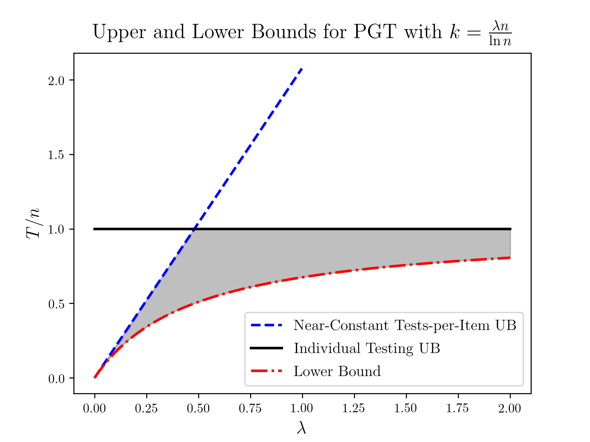
Figure 1: Comparison of upper and lower bounds for PGT in the regime where $k=\lambda n/\log n$. The shaded region indicates the gap between the current upper and lower bounds.

A natural next step would be to close this gap. In the sparse regime where $k=O(n^{\theta})$, more complex decodings known as DD and SPIV have been shown to improve on the COMP decoding [21, 22], although the benefit seems to vanish as $\theta$ approaches 1.

We conjecture that the lower bound should come up to meet the upper bound obtained by the minimum of near-constant tests-per-item designs and individual testing. This would imply that the exact point at which individual testing becomes suboptimal is when $p<(\log 2)^{2}/\log n$.

The reason for this belief is as follows. Suppose $D$ is the (random) number of disguised items. A simple calculation shows that,

$$\mathbb{E}[D]\geq n\exp(T/n\cdot\mathcal{L}_{p})$$

where $\mathcal{L}_{p}$ has been defined in the last section. Using the same calculation as before, we obtain,

$$\mathbb{E}[D]\geq n2^{-\frac{T}{n}\frac{\log 2}{p}}.$$

Given the number of disguised items is $D$, the probability of correct decoding is at most $(1-p)^{D}\leq\exp(-pD),$ where $p=\frac{\lambda}{\log n}$. Substituting $D$ with $\mathbb{E}D$ from above, we see that the probability of correct decoding is going to zero whenever $\frac{T}{n}<\frac{\lambda}{\log^{2}2}.$ This shows that the lower bound should be improved to match the upper bound, if the random variable $D$ is concentrated around its mean, which is of course yet to be proved.

References

- [1] R. Dorfman, “The detection of defective members of large populations,” The Annals of Mathematical Statistics, vol. 14, no. 4, pp. 436–440, 1943.
- [2] I. Yelin, N. Aharony, E. S. Tamar, A. Argoetti, E. Messer, D. Berenbaum, E. Shafran, A. Kuzli, N. Gandali, O. Shkedi et al., “Evaluation of covid-19 rt-qpcr test in multi sample pools,” Clinical Infectious Diseases, vol. 71, no. 16, pp. 2073–2078, 2020.
- [3] C. Gollier and O. Gossner, “Group testing against covid-19,” EconPol Policy Brief, Tech. Rep., 2020.
- [4] J. N. Eberhardt, N. P. Breuckmann, and C. S. Eberhardt, “Multi-stage group testing improves efficiency of large-scale covid-19 screening,” Journal of Clinical Virology, vol. 128, p. 104382, 2020.
- [5] D. Du and F. Hwang, Combinatorial Group Testing and Its Applications, ser. Applied Mathematics. World Scientific, 2000. [Online]. Available: https://books.google.com/books?id=KW5-CyUUOggC
- [6] C. L. Chan, P. H. Che, S. Jaggi, and V. Saligrama, “Non-adaptive probabilistic group testing with noisy measurements: Near-optimal bounds with efficient algorithms,” in 2011 49th Annual Allerton Conference on Communication, Control, and Computing (Allerton). IEEE, 2011, pp. 1832–1839.
- [7] A. Sebő, “On two random search problems,” Journal of Statistical Planning and Inference, vol. 11, no. 1, pp. 23–31, 1985.
- [8] G. K. Atia and V. Saligrama, “Boolean compressed sensing and noisy group testing,” Information Theory, IEEE Transactions on, vol. 58, no. 3, pp. 1880–1901, 2012.
- [9] A. Mazumdar, “Nonadaptive group testing with random set of defectives,” IEEE Trans. Information Theory, vol. 62, no. 12, pp. 7522–7531, 2016.
- [10] A. Barg and A. Mazumdar, “Group testing schemes from codes and designs,” IEEE Transactions on Information Theory, vol. 63, no. 11, pp. 7131–7141, 2017.
- [11] H. A. Inan, P. Kairouz, M. Wootters, and A. Özgür, “On the optimality of the kautz-singleton construction in probabilistic group testing,” IEEE Transactions on Information Theory, vol. 65, no. 9, pp. 5592–5603, 2019.
- [12] S. Cai, M. Jahangoshahi, M. Bakshi, and S. Jaggi, “Efficient algorithms for noisy group testing,” IEEE Transactions on Information Theory, vol. 63, no. 4, pp. 2113–2136, 2017.
- [13] A. Vem, N. T. Janakiraman, and K. R. Narayanan, “Group testing using left-and-right-regular sparse-graph codes,” arXiv preprint arXiv:1701.07477, 2017.
- [14] K. Lee, K. Chandrasekher, R. Pedarsani, and K. Ramchandran, “Saffron: A fast, efficient, and robust framework for group testing based on sparse-graph codes,” IEEE Transactions on Signal Processing, vol. 67, no. 17, pp. 4649–4664, 2019.
- [15] S. Bondorf, B. Chen, J. Scarlett, H. Yu, and Y. Zhao, “Sublinear-time non-adaptive group testing with o (klogn) tests via bit-mixing coding,” IEEE Transactions on Information Theory, 2020.
- [16] H. A. Inan and A. Ozgur, “Strongly explicit and efficiently decodable probabilistic group testing,” in 2020 IEEE International Symposium on Information Theory (ISIT). IEEE, 2020, pp. 525–530.
- [17] A. Agarwal, S. Jaggi, and A. Mazumdar, “Novel impossibility results for group-testing,” in 2018 IEEE International Symposium on Information Theory (ISIT). IEEE, 2018, pp. 2579–2583.
- [18] M. Aldridge, “Individual testing is optimal for nonadaptive group testing in the linear regime,” IEEE Transactions on Information Theory, vol. 65, no. 4, pp. 2058–2061, 2018.
- [19] J. Scarlett and V. Cevher, “Limits on support recovery with probabilistic models: An information-theoretic framework,” IEEE Transactions on Information Theory, vol. 63, no. 1, pp. 593–620, 2016.
- [20] M. Aldridge, “The capacity of bernoulli nonadaptive group testing,” IEEE Transactions on Information Theory, vol. 63, no. 11, pp. 7142–7148, 2017.
- [21] O. Johnson, M. Aldridge, and J. Scarlett, “Performance of group testing algorithms with near-constant tests per item,” IEEE Transactions on Information Theory, vol. 65, no. 2, pp. 707–723, 2018.
- [22] A. Coja-Oghlan, O. Gebhard, M. Hahn-Klimroth, and P. Loick, “Optimal group testing,” in Conference on Learning Theory. PMLR, 2020, pp. 1374–1388.
- [23] M. Aldridge, O. Johnson, and J. Scarlett, “Group testing: an information theory perspective,” arXiv preprint arXiv:1902.06002, 2019.
- [24] W. H. Bay, E. Price, and J. Scarlett, “Optimal non-adaptive probabilistic group testing requires tests,” arXiv e-prints, pp. arXiv–2006, 2020.