Affine OneMax

Abstract

A new class of test functions for black box optimization is introduced. Affine OneMax (AOM) functions are defined as compositions of OneMax and invertible affine maps on bit vectors. The black box complexity of the class is upper bounded by a polynomial of large degree in the dimension. The proof relies on discrete Fourier analysis and the Kushilevitz-Mansour algorithm. Tunable complexity is achieved by expressing invertible linear maps as finite products of transvections. The black box complexity of sub-classes of AOM functions is studied. Finally, experimental results are given to illustrate the performance of search algorithms on AOM functions.

Keywords: Combinatorial optimization, black box optimization, test functions, tunable complexity, linear group, transvections, black box complexity, discrete Fourier analysis

1 Introduction

Theoretical and empirical analyses of search algorithms in the context of black box optimization often require test functions. On the practical side, an algorithm is usually selected by its performance across a collection of diverse test functions such as OneMax, LeadingOnes, MaxSat, etc. In particular, NK landscapes [17] are a class of functions with tunable complexity. In this model, the fitness of an $n$-dimensional bit vector is the sum of $n$ partial functions, one per variable. Each partial function depends on a variable and its $k$ neighbors. The number $k$ controls the interaction graph hence the complexity of the fitness landscape. NK landscapes have found many applications from theoretical biology to combinatorial optimization. When used as test functions, their flexibility comes at the price of a great number of parameters. Values of partial functions are often sampled from normal or uniform distributions, which generates highly irregular landscapes with unknown maximum, even for small $k$.

Affine OneMax (AOM) functions are test functions defined as compositions of OneMax and invertible affine maps on bit vectors. They are integer-valued, have a known maximum, and their representations only require a number of bits quadratic in the dimension. The idea of composition of a fitness function and a linear or affine map has already been explored in the context of evolutionary computation [20, 21, 24]. The problem addressed in this line of research is to identify a representation of the search space, e.g. an affine map, able to transform a deceptive function into an easy one for genetic algorithms. In Sec. 4, we propose an algorithm which learns such a representation for AOM functions. Considering the identity as a linear map, it appears that functions of increasing complexity can be obtained starting with the identity and applying small perturbations to it. In the language of group theory, those perturbations are called elementary (or special) transvections. Sequences of elementary transvections are multiplied to obtain arbitrary linear maps. The key parameter of resulting AOM functions is the sequence length which is the analogue of parameter $k$ in NK landscapes.

The theory of black box complexity [6, 5] usually involves classes of functions rather than single functions. The black box complexity $B_{\mathcal{F}}$ of a class $\mathcal{F}$ of functions is defined as $\inf_{A\in\mathcal{A}}\sup_{f\in\mathcal{F}}\allowbreak\operatorname{\mathbb{E}}(T(A,f))$, where $\mathcal{A}$ is the set of randomized search algorithms and $\operatorname{\mathbb{E}}(T(A,f))$ the expected runtime of algorithm $A$ on function $f$. We will only consider unrestricted randomized search algorithms hence unrestricted black box complexity. The usual way to devise a function class is to supplement a given function with modified versions of it. For example, instead of OneMax alone, it is customary to consider the function class comprising all compositions of OneMax with linear permutations (permutation of variables) and translations. Given the fact that linear permutations and translations are invertible affine maps, it seems natural to consider all invertible affine maps. In this paper, we prove that the black box complexity of AOM functions is upper bounded by $O(n^{10}\log^{2}n)$. The proof uses the Kushilevitz-Mansour algorithm [19] which is an application of discrete Fourier (or Walsh) analysis to the approximation of Boolean functions. Fourier analysis has been extensively used in the analysis of genetic algorithms [8] or fitness landscapes [27, 12, 11]. It also plays an important role in the construction of a search matrix in the analysis [3] of the coin weighing problem [7] which is related to OneMax.

The paper is organized as follows. Sec. 2 introduces general AOM functions and gives their basic properties. Sec. 3 introduces elementary transvections and their products. Sec. 4 addresses the black box complexity of AOM functions. In Sec. 5, we report results of experiments involving search algorithms on random instances. Sec. 6 concludes the paper.

2 General case

The OneMax function $\ell:\{0,1\}^{n}\rightarrow\mathbb{R}$ is defined by $\ell(x)=\sum_{i=1}^{n}x_{i}$, where the $x_{i}$’s are seen as real numbers. OneMax takes $n+1$ values $0,1,\ldots,n$ and, for all $k\in[0..n]$, $|\ell^{-1}(k)|=\binom{n}{k}$. It reaches its maximum $n$ only at $1^{n}=(1,1,\ldots,1)$.

From now on, the set $\{0,1\}$ is seen as the finite field $\mathbb{F}_{2}$ ($1+1\equiv 0\pmod{2}$) and $\{0,1\}^{n}$ as a linear space over $\mathbb{F}_{2}$. The canonical basis of $\{0,1\}^{n}$ is denoted by $(e_{i})$, where $i\in[1..n]$. An affine map $\{0,1\}^{n}\rightarrow\{0,1\}^{n}$ is defined by $x\mapsto Mx+b$, where $M$ is a $n\times n$ bit matrix and $b$ a $n\times 1$ bit vector. Sums and products in $Mx+b$ are computed in $\mathbb{F}_{2}$ not in $\mathbb{R}$.

Definition and basic properties

An affine OneMax function $f$ is the composition of OneMax and an invertible affine map. More precisely, it is defined by $f(x)=\ell(Mx+b)$, where $M\in\operatorname{GL}(n,\mathbb{F}_{2})$, that is $M$ is an invertible matrix. The invertibility of $M$ is important because it ensures that $f$ shares the properties of OneMax outlined above. Firstly, it takes $n+1$ values $0,1,\ldots,n$ and, for all $k\in[0..n]$, $|f^{-1}(k)|=\binom{n}{k}$. Secondly, it reaches its maximum $n$ only once at $x^{*}$ such that $Mx^{*}+b=1^{n}$ or $x^{*}=M^{-1}(1^{n}+b)$. The set of all AOM functions will be denoted by $\mathcal{F}$. By construction, $\mathcal{F}$ is closed under invertible affine maps but

Theorem 1.

$\mathcal{F}$ is not closed under permutations.

Proof.

Let $f=\ell\in\mathcal{F}$ and $\pi$ the (nonlinear) permutation of $\{0,1\}^{n}$ which exchanges $0$ and $e_{1}$ and leaves other vectors unchanged. We will prove by reductio ad absurdum that $f\circ\pi$ does not belong to $\mathcal{F}$. Suppose that $g=f\circ\pi\in\mathcal{F}$. Then, there exists $(M,b)\in\operatorname{GL}(n,\mathbb{F}_{2})\times\{0,1\}^{n}$ such that, for all $x\in\{0,1\}^{n}$, $g(x)=\ell(Mx+b)$. We will need $g(0)$, $g(e_{1})$, $g(e_{2})$, and $g(e_{3})$. We have $g(0)=(\ell\circ\pi)(0)=\ell(e_{1})=1$ and $g(0)=\ell(b)$. Then, there exists $i_{1}\in[1..n]$ such that $b=e_{i_{1}}$. We have $g(e_{1})=(\ell\circ\pi)(e_{1})=\ell(0)=0$ and $g(e_{1})=\ell(Me_{1}+b)$. Then, $Me_{1}+b=0\Leftrightarrow Me_{1}=b=e_{i_{1}}$. We have $g(e_{2})=(\ell\circ\pi)(e_{2})=\ell(e_{2})=1$ and $g(e_{2})=\ell(Me_{2}+b)$. Then, there exists $i_{2}\in[1..n]$ such that $Me_{2}+b=e_{i_{2}}\Leftrightarrow Me_{2}=e_{i_{1}}+e_{i_{2}}$. Similarly, there exists $i_{3}\in[1..n]$ such that $Me_{3}=e_{i_{1}}+e_{i_{3}}$. To reach a contradiction, we consider $x=e_{2}+e_{3}$. We have $g(x)=(\ell\circ\pi)(x)=\ell(x)=2$ and $g(x)=\ell(Mx+b)=\ell(Me_{2}+Me_{3}+b)=\ell(e_{i_{1}}+e_{i_{2}}+e_{i_{3}})$ which is necessarily odd. We conclude that $f\circ\pi$ does not belong to $\mathcal{F}$. ∎

As a consequence, by a NFL theorem [26], the average performance of an algorithm over all AOM functions depends on the algorithm. Finally, we state a property relating AOM functions and linear permutations. Let $\Phi:\operatorname{GL}(n,\mathbb{F}_{2})\times\{0,1\}^{n}\to\mathcal{F}$ be the map defined by $\Phi(M,b)=f$, where $f(x)=\ell(Mx+b)$. Then, for all $(M,b)$ and all linear permutations $\pi$, $\Phi(\pi M,\pi b)=\Phi(M,b)$. This is a direct consequence of the fact that OneMax itself is invariant under linear permutations, that is, for all linear permutations $\pi$, $\ell\circ\pi=\ell$. Given an AOM function $\Phi(M,b)$, an algorithm can only learn $M$ and $b$ up to a linear permutation.

To sample a random AOM function, one has to sample an invertible matrix and a vector. An invertible matrix can be sampled by means of rejection sampling. The success probabiblity $p_{n}$ is equal to $|\operatorname{GL}(n,\mathbb{F}_{2})|/2^{n^{2}}$, where $|\operatorname{GL}(n,\mathbb{F}_{2})|=(2^{n}-2^{0})(2^{n}-2^{1})\cdots(2^{n}-2^{n-1})$ and $2^{n^{2}}$ is the number of $n\times n$ matrices. By a convexity argument, $\ln p_{n}=\sum_{k=1}^{n}\ln(1-2^{-k})\geq-2\ln 2(1-2^{-n})\geq-2\ln 2$. Thus, the expected number of trials to sample an invertible matrix is bounded from above by 4.

Fourier analysis

Let $\mathcal{E}$ denote the space of pseudo-Boolean functions. For all functions $f,g\in\mathcal{E}$, define their inner product by $\langle f,g\rangle=2^{-n}\sum_{x}f(x)\cdot g(x)$, where the sum ranges over $\{0,1\}^{n}$. It will be useful to interpret inner products as expectations. More precisely, $\langle f,g\rangle=\operatorname{\mathbb{E}}(fg)=\operatorname{\mathbb{E}}(f(X)g(X))$, where $X$ is a random vector with uniform distribution on $\{0,1\}^{n}$. For all $x,u\in\{0,1\}^{n}$, let $\chi_{u}(x)=(-1)^{x\cdot u}$, where $x\cdot u=\sum_{i}x_{i}u_{i}$. The $\chi_{u}$’s define an orthonormal basis of $\mathcal{E}$. For all functions $f\in\mathcal{E}$, $f=\sum_{u}\lambda_{u}\chi_{u}$, where $\lambda_{u}=\langle f,\chi_{u}\rangle$. The set of coefficients $\lambda_{u}$ is called the spectrum of $f$. The coefficient $\lambda_{0}$ is equal to the average value of $f$. A function $f$ is $t$-sparse if it has at most $t$ nonzero coefficients. The Fourier transform $\widehat{f}$ of $f$ is defined by $\widehat{f}(u)=\lambda_{u}$. The support of $\widehat{f}$ is called the set of feature vectors of $f$.

The computation of the spectrum of OneMax gives the nonzero coefficients $\widehat{\ell}(0)=n/2$ and $\widehat{\ell}(e_{i})=-1/2$. If we discard $\widehat{\ell}(0)$, we can consider that it is made of $n$ nonzero coefficients of equal amplitude, one for each basis vector. In order to compute the spectrum of an AOM function, we use the known properties of Fourier transform relative to linear maps and translations. For all $f\in\mathcal{E}$ and $M\in\operatorname{GL}(n,\mathbb{F}_{2})$, if $g=f\circ M$ then $\widehat{g}=\widehat{f}\circ(M^{-1})^{\intercal}$. For all $b\in\{0,1\}^{n}$, let $T_{b}:\{0,1\}^{n}\rightarrow\{0,1\}^{n}$ be the translation defined by $T_{b}(x)=x+b$. If $g=f\circ T_{b}$ then $\widehat{g}(u)=(-1)^{u\cdot b}\widehat{f}(u)$.

Now, let $f=\Phi(M,b)$ be an AOM function. Then, $f=(\ell\circ T_{b})\circ M$, $\widehat{f}=\widehat{(\ell\circ T_{b})}\circ(M^{-1})^{\intercal}$, and $\widehat{f}(u)=\widehat{(\ell\circ T_{b})}(v)=(-1)^{v\cdot b}\widehat{\ell}(v)$, where $v=(M^{-1})^{\intercal}u$. Combining the last result with the spectrum of $\ell$ and solving for $u$ in the equations $(M^{-1})^{\intercal}u=e_{i}$, we obtain the nonzero coefficients $\widehat{f}(0)=n/2$ and $\widehat{f}(M^{\intercal}e_{i})=-(-1)^{b_{i}}/2$. The spectrum of AOM functions is similar to that of OneMax (same number of nonzero coefficients and same amplitudes). There is an additional phase factor $(-1)^{b_{i}}$ but the most important difference is that a nonzero feature vector can now be any nonzero vector instead of just one of the basis vectors. More precisely, the nonzero feature vectors of $f$ are the rows of $M$. Given that $M$ is invertible, they can form any basis of $\{0,1\}^{n}$. As a consequence, AOM functions are not bounded in the sense that if $u$ is a nonzero feature vector of an AOM function then $\ell(u)$ can take any value in $[1..n]$.

3 Tunable complexity

We would like to sort AOM functions from the easiest to the hardest ones to maximize or at least provide them with some structure. We will achieve this goal using transvections. A transvection is an invertible linear map $\{0,1\}^{n}\rightarrow\{0,1\}^{n}$ defined by $x\mapsto x+h(x)a$, where $h$ is a non constant linear form and $a\neq 0$ a vector such that $h(a)=0$. Transvections generate the special linear group $\operatorname{SL}(n,\mathbb{F}_{2})$ which is represented by the group of matrices of determinant 1. Since being $=1$ is the same as being $\neq 0$ in $\mathbb{F}_{2}$, the special linear group $\operatorname{SL}(n,\mathbb{F}_{2})$ is also the general linear group $\operatorname{GL}(n,\mathbb{F}_{2})$ of invertible linear maps. In the general case, the inverse of $x\mapsto x+h(x)a$ is $x\mapsto x-h(x)a$. In the case of $\mathbb{F}_{2}$, a transvection is equal to its own inverse.

We concentrate on particular transvections called elementary transvections. For all $i,j\in[1..n]$, with $i\neq j$, let $\tau_{ij}$ denote an elementary transvection. For all $x\in\{0,1\}^{n}$, $\tau_{ij}x$ is obtained from $x$ by adding $x_{j}$ to $x_{i}$ or $x_{i}\leftarrow x_{i}+x_{j}$, leaving other bits unchanged. At most one bit is changed. It is clear that $\tau_{ij}$ is a linear map. Its matrix is defined by $I_{n}+B_{ij}$, where $I_{n}$ is the $n\times n$ identity matrix and $B_{ij}$ is the matrix whose $(i,j)$ entry is 1 and other entries are zero. Throughout the remainder of this paper, we will write transvection to mean elementary transvection. For all disjoint pairs $\{i,j\}$ and $\{k,l\}$, the transvections $\tau_{ij}$ and $\tau_{kl}$ commute, that is, $\tau_{ij}\tau_{kl}=\tau_{kl}\tau_{ij}$. Such transvections will be said disjoint. We have already seen that $\tau_{ij}^{2}=I_{n}$. For all sets $\{i,j,k\}$, $\tau_{ij}$ and $\tau_{ik}$ (same destination) commute, $\tau_{ik}$ and $\tau_{jk}$ (same source) commute, but $\tau_{ij}$ and $\tau_{jk}$ do not.

Having defined transvections, we consider finite products of transvections, gradually increasing the requirements, and the corresponding classes of AOM functions. Let $t$ be a positive integer. Let $G_{t}$ be the set of all products of $t$ transvections. Let $G_{t}^{c}$ be the set of all products of $t$ (pairwise) commuting transvections. Let $M=\prod_{k=1}^{t}\tau_{i_{k}j_{k}}$, $I$ be the set of destination indices, and $J$ be the set of source indices. The transvections are commuting if and only if the sets $I$ and $J$ are disjoint. Consequently, the set $G_{t}^{c}$ is defined (non empty) for all $t\in[1..\lfloor n^{2}/4\rfloor]$. Let $G_{t}^{\delta}$ be the set of all products of $t$ commuting transvections where each source index appears at most once. In this case, for all products, we can define a function $\delta$ from sources $J$ to destinations $I$. Let $G_{t}^{\sigma}$ be the set of all products of $t$ commuting transvections where each destination index appears at most once. In this case, for all products, we can define a function function $\sigma$ from destinations $I$ to sources $J$. Both sets $G_{t}^{\delta}$ and $G_{t}^{\sigma}$ are defined for all $t\in[1..(n-1)]$. Finally, for all $t\in[1..\lfloor n/2\rfloor]$, let $G_{t}^{d}$ be the set of all products of $t$ disjoint transvections. We have the inclusions $G_{t}^{d}\subset G_{t}^{\delta},G_{t}^{\sigma}\subset G_{t}^{c}\subset G_{t}\subset\operatorname{GL}(n,\mathbb{F}_{2})$.

We define function classes corresponding to sets of transvection products. Let $\mathcal{F}_{t}$ be the set of functions $x\mapsto\ell(Mx+b)$, where $M\in G_{t}$ and $b\in\{0,1\}^{n}$. Classes $\mathcal{F}_{t}^{c}$, $\mathcal{F}_{t}^{\sigma}$, $\mathcal{F}_{t}^{\delta}$, and $\mathcal{F}_{t}^{d}$ are defined similarly. We have the inclusions $\mathcal{F}_{t}^{d}\subset\mathcal{F}_{t}^{\delta},\mathcal{F}_{t}^{\sigma}\subset\mathcal{F}_{t}^{c}\subset\mathcal{F}_{t}\subset\mathcal{F}$. Functions in classes $\mathcal{F}_{t}$ will be refered to as transvection sequence AOM (TS-AOM) functions.

As in the general case, we need to sample random TS-AOM functions in $\mathcal{F}_{t}$. We propose to sample uniformly distributed random sequences of $t$ transvections. However, the distribution of their products is not uniform on $G_{t}$ and the distribution of resulting functions is not uniform on $\mathcal{F}_{t}$.

4 Black box complexity

Let us first study the black box complexity of general AOM functions. We will give an upper bound of $B_{\mathcal{F}}$ by means of a randomized search algorithm which efficiently learns and maximizes AOM functions. Sparsity is the most important property of AOM functions. It reminds us of Boolean functions which can be efficiently approximated by sparse functions using the Kushilevitz-Mansour (KM) algorithm [19]. Indeed, we will prove that the KM algorithm can efficiently learn the spectrum of AOM functions. In the theory of fitness landscapes, most algorithms apply to bounded functions such as NK landscapes [4]. However, as explained at the end of Sec. 2, AOM functions are not bounded, hence the interest of the KM algorithm.

AOM functions are not Boolean functions so we need to transform them before applying the KM algorithm.

Lemma 1.

Let $\mathcal{G}=\{2f/n-1:f\in\mathcal{F}\}$. If $g\in\mathcal{G}$ then $g$ has the following properties:

1. For all $x\in\{0,1\}^{n}$, $|g(x)|\leq 1$.

2. $g$ is $n$-sparse.

3. For all $u\in\{0,1\}^{n}$, $\widehat{g}(u)=0$ or $|\widehat{g}(u)|=1/n$.

4. $\operatorname{\mathbb{E}}(g^{2})=1/n$.

We state the key definition and lemma from the work of Kushilevitz and Mansour needed to understand their algorithm.

Definition 1.

For all $g\in\mathcal{G}$, all $k\in[1..n-1]$, and all $u\in\{0,1\}^{k}$, the function $g_{u}:\{0,1\}^{n-k}\rightarrow\mathbb{R}$ is defined by $g_{u}(x)=\sum_{v\in\{0,1\}^{n-k}}\widehat{g}(uv)\chi_{v}(x)$, where $uv$ is the concatenation of $u$ and $v$.

Lemma 2.

For all $g\in\mathcal{G}$ and all $k\in[1..n-1]$, the following properties are satisfied:

1. For all $u\in\{0,1\}^{k}$, $\operatorname{\mathbb{E}}(g_{u}^{2})=\sum_{v\in\{0,1\}^{n-k}}(\widehat{g}(uv))^{2}$.

2. $\sum_{u\in\{0,1\}^{k}}\operatorname{\mathbb{E}}(g_{u}^{2})=\allowbreak\operatorname{\mathbb{E}}(g^{2})$.

3. For all $u\in\{0,1\}^{k}$ and all $x\in\{0,1\}^{n-k}$, $g_{u}(x)=\operatorname{\mathbb{E}}(g(Yx)\cdot\chi_{u}(Y))$, where $Y$ is a random vector with uniform distribution on $\{0,1\}^{k}$, and $|g_{u}(x)|\leq 1$.

Algorithm 1 Kushilevitz-Mansour algorithm

1:  $\text{KM}(g,m_{1},m_{2},u)$:

2:  $k\leftarrow\text{length}(u)$

3:  for all $i\in[1..m_{1}]$ do

4:     sample $x_{i}\in\{0,1\}^{n-k}$

5:     for all $j\in[1..m_{2}]$ do

6:        sample $y_{i,j}\in\{0,1\}^{k}$

7:     end for

8:     $A_{i}\leftarrow(1/m_{2})\sum_{j=1}^{m_{2}}g(y_{i,j}x_{i})\chi_{u}(y_{i,j})$

9:  end for

10:  $B_{u}\leftarrow(1/m_{1})\sum_{i=1}^{m_{1}}A_{i}^{2}$

11:  if $B_{u}>1/(2n^{2})$ then

12:     if $k=n$ then

13:        return  $\{u\}$

14:     else

15:        $U_{0}\leftarrow\text{KM}(g,m_{1},m_{2},u0)$

16:        $U_{1}\leftarrow\text{KM}(g,m_{1},m_{2},u1)$

17:        return  $U_{0}\cup U_{1}$

18:     end if

19:  else

20:     return  $\emptyset$

21:  end if

The Kushilevitz-Mansour algorithm (see Alg. 1) follows a depth-first search of the complete binary tree of depth $n$. In this context, $u\in\{0,1\}^{k}$ can be seen as a prefix or a path from the root to an internal node of the tree. The expectation $\operatorname{\mathbb{E}}(g_{u}^{2})$ simply counts the number of leaves below $u$ and labelled by feature vectors. If it is lower than $1/n^{2}$ then there is no need to expand the node. However, expectations such as $\operatorname{\mathbb{E}}(g_{u}^{2})$ cannot be computed efficiently so that a random approximation is required. We will use Hoeffding’s inequality [15] to control the concentration of sample averages around their expectations.

Lemma 3 (Hoeffding).

Let $Z_{1}$, $Z_{2}$, …, $Z_{m}$ be independent random variables such that, for all $i\in[1..m]$, $a_{i}\leq Z_{i}\leq b_{i}$, $c_{i}=b_{i}-a_{i}$, and $\operatorname{\mathbb{E}}(Z_{i})=\mu$. Let $\overline{Z}=(1/m)\sum_{i=1}^{m}Z_{i}$. Then, for all positive real numbers $d$, $\operatorname{\mathbb{P}}(|\overline{Z}-\mu|\geq d)\leq 2\exp(-2m^{2}d^{2}/\sum_{i=1}^{m}c_{i}^{2})$.

We state and prove a series of lemmas leading to the main theorem and its corollary. This is adapted from the work of Kushilevitz and Mansour to the case of AOM functions instead of Boolean functions.

Lemma 4.

Let $m_{1}\in\mathbb{N}^{*}$ and $X_{1}$, $X_{2}$, …, $X_{m_{1}}$ be independent random vectors with uniform distribution on $\{0,1\}^{n-k}$. Let $B_{u}^{\prime}=(1/m_{1})\sum_{i=1}^{m_{1}}g_{u}^{2}(X_{i})$. Then

$$\operatorname{\mathbb{P}}(|B_{u}^{\prime}-\operatorname{\mathbb{E}}(g_{u}^{2})|\geq 1/(4n^{2}))\leq 2\exp(-m_{1}/(8n^{4}))\,.$$

Proof.

Apply Hoeffding’s inequality with $m=m_{1}$, $Z_{i}=g_{u}^{2}(X_{i})$, $\mu=\operatorname{\mathbb{E}}(g_{u}^{2})$, $a_{i}=0$, $b_{i}=1$, $c_{i}=1$, and $d=1/(4n^{2})$. ∎

Lemma 5.

Let $m_{1},m_{2}\in\mathbb{N}^{*}$ and, for all $i\in[1..m_{1}]$, let $Y_{i,1}$, $Y_{i,2}$, …, $Y_{i,m_{2}}$ be independent random vectors with uniform distribution on $\{0,1\}^{k}$. For all $x\in\{0,1\}^{n-k}$, let $A_{i}(x)=(1/m_{2})\sum_{j=1}^{m_{2}}g(Y_{i,j}x)\cdot\chi_{u}(Y_{i,j})$. Then

$$\operatorname{\mathbb{P}}(|A_{i}(x)-g_{u}(x)|\geq 1/(8n^{2}))\leq 2\exp(-m_{2}/(128n^{4}))\,.$$

Proof.

We apply Hoeffding’s inequality with $m=m_{2}$, $Z_{j}=g(Y_{i,j}x)\cdot\chi_{u}(Y_{i,j})$, $\mu=g_{u}(x)$, $a_{i}=-1$, $b_{i}=1$, $c_{i}=2$, and $d=1/(8n^{2})$. ∎

Lemma 6.

Let $B_{u}=(1/m_{1})\sum_{i=1}^{m_{1}}A_{i}^{2}(X_{i})$. If, for all $i\in[1..n]$ and all $x\in\{0,1\}^{n-k}$, $|A_{i}(x)-g_{u}(x)|<1/(8n^{2})$ then $|B_{u}-B_{u}^{\prime}|<1/(4n^{2})$.

Proof.

$$B_{u}-B_{u}^{\prime} =(1/m_{1})\sum_{i=1}^{m_{1}}(A_{i}^{2}(X_{i})-g_{u}^{2}(X_{i}))$$

$$=(1/m_{1})\sum_{i=1}^{m_{1}}(A_{i}(X_{i})-g_{u}(X_{i}))\times(A_{i}(X_{i})+g_{u}(X_{i}))$$

Since both $g_{u}$ and $A_{i}$ are bounded in $[-1,1]$, then

$$|B_{u}-B_{u}^{\prime}|\leq(2/m_{1})\sum_{i=1}^{m_{1}}|A_{i}(X_{i})-g_{u}(X_{i})|<1/(4n^{2})\,.$$

∎

Lemma 7.

Let $m_{3}\in\mathbb{N}^{*}$ and $h=2f-n$. For all $i\in[1..n]$ and all $u\in\{0,1\}^{n}$, let $X_{i,1}$, $X_{i,2}$, …, $X_{i,m_{3}}$ be independent random vectors with uniform distribution on $\{0,1\}^{n}$ and $C_{i}=(1/m_{3})\sum_{j=1}^{m_{3}}h(X_{i,j})\cdot\chi_{u}(X_{i,j})$. Then $\operatorname{\mathbb{P}}(|C_{i}-\widehat{h}(u)|\geq 1)\leq 2\exp(-m_{3}/(2n^{2}))$.

Proof.

Apply Hoeffding’s inequality with $m=m_{3}$, $Z_{j}=h(X_{i,j})\cdot\chi_{u}(X_{i,j})$, $\mu=\widehat{h}(u)$, $a_{i}=-n$, $b_{i}=n$, $c_{i}=2n$, and $d=1$. ∎

Theorem 2.

Let $f\in\mathcal{F}$ and $\delta\in(0,1)$. There is a randomized algorithm which exactly learns and maximizes $f$ with at most $m_{1}m_{2}n^{2}+m_{3}n$ evaluations and probability at least $1-\delta$, where $m_{1}=\Theta\left(n^{4}\log(n^{2}/\delta)\right)$, $m_{2}=\Theta\left(n^{4}\log(n^{2}m_{1}/\delta)\right)$, $m_{3}=\Theta\left(n^{2}\log(n/\delta)\right)$.

Algorithm 2 Algorithm for $\mathcal{F}$

1:  $\text{Maximize}(f,m_{1},m_{2},m_{3})$:

2:  $g\leftarrow 2f/n-1$

3:  $U\leftarrow\text{KM}(g,m_{1},m_{2},\emptyset)$

4:  $h\leftarrow 2f-n$

5:  for all $i\in[1..n]$ do

6:     for all $j\in[1..m_{3}]$ do

7:        sample $x_{i,j}\in\{0,1\}^{n}$

8:     end for

9:     $C_{i}\leftarrow(1/m_{3})\sum_{j=1}^{m_{3}}h(x_{i,j})\chi_{u_{i}}(x_{i,j})$

10:     if $C_{i}>0$ then

11:        $b_{i}\leftarrow 1$

12:     else

13:        $b_{i}\leftarrow 0$

14:     end if

15:  end for

16:  $M\leftarrow(u_{1},u_{2},\ldots,u_{n})^{\intercal}$

17:  return  $M^{-1}(1^{n}+b)$

Proof.

Alg. 2 first calls Alg. 1 to determine all $n$ nonzero feature vectors of $f$, then estimates $b$ before returning the solution. We arbitrarily divide the error probability $\delta$ into $\delta/2$ for KM and $\delta/2$ for learning $b$. It is further divided into $\delta/(2n^{2})$ per recursive call in KM and $\delta/(2n)$ per component of $b$. Finally, $\delta/(4n^{2})$ is allocated to the computation of $B_{u}$ and $\delta/(4n^{2}m_{1})$ to that of each $A_{i}$. With the probability bound in Lemma 4, the condition $2\exp(-m_{1}/(8n^{4}))=\delta/(4n^{2})$ gives $m_{1}=\Theta\left(n^{4}\log(n^{2}/\delta)\right)$. With the probability bound in Lemma 5, the condition $2\exp(-m_{2}/(128n^{4}))=\delta/(4n^{2}m_{1})$ gives $m_{2}=\Theta\left(n^{4}\log(n^{2}m_{1}/\delta)\right)$. Finally, with the probability bound in Lemma 7, the condition $2\exp(-m_{3}/(2n^{2}))=\delta/(2n)$ gives $m_{3}=\Theta\left(n^{2}\log(n/\delta)\right)$. With probability at least $1-\delta$, every sample average is sufficiently concentrated around its mean. In this case, in every call to KM, $|B_{u}-\operatorname{\mathbb{E}}(g_{u}^{2})|\leq|B_{u}-B_{u}^{\prime}|+|B_{u}^{\prime}-\operatorname{\mathbb{E}}(g_{u}^{2})|<1/(4n^{2})+1/(4n^{2})=1/(2n^{2})$, where $\operatorname{\mathbb{E}}(g_{u}^{2})=0$ or $\operatorname{\mathbb{E}}(g_{u}^{2})\geq 1/n^{2}$. Similarly, every inequality $|C_{i}-\widehat{h}(u)|<1$ is satisfied, where $\widehat{h}(u)=-1$ or 1. As a consequence, Alg. 2 correctly learns and maximizes $f$ with probability at least $1-\delta$. The number of recursive calls in KM is at most $n^{2}$ and each one of them requires $m_{1}m_{2}$ evaluations. Moreover, $b$ has $n$ components and each one of them requires $m_{3}$ evaluations. ∎

Corollary 1.

$B_{\mathcal{F}}=O(n^{10}\log^{2}n)$.

Proof.

We repeatedly run Alg. 2 until a maximal point is found. The expected total number of evaluations is at most $(m_{1}m_{2}n^{2}+m_{3}n)/(1-\delta)$. Arbitrarily setting $\delta=1/2$ leads to $m_{1}m_{2}=\Theta(n^{8}\cdot\log^{2}n)$ and the announced upper bound. ∎

Theorem 3.

$B_{\mathcal{F}}=\Omega(n/\log n)$.

Proof.

AOM functions take all $n+1$ values $0,1,\ldots,n$. For each $x\in\{0,1\}^{n}$, there exists $f\in\mathcal{F}$ such that $x$ is its maximal point, which is equivalent to the fact that the set $\{(M,b)\in\operatorname{GL}(n,\mathbb{F}_{2})\times\{0,1\}^{n}:Mx+b=1^{n}\}$ is not empty. For example, choose any $M\in\operatorname{GL}(n,\mathbb{F}_{2})$ and set $b=Mx+1^{n}$. By Theorem 2 in [6], $B_{\mathcal{F}}=\Omega(\log_{n}2^{n})=\Omega(n/\log n)$. ∎

Let us now study the black box complexity of TS-AOM functions with small sequence length.

Theorem 4.

Let $\mathcal{F}_{1}^{0}=\{\ell\circ\tau:\tau\in G_{1}\}\subset\mathcal{F}_{1}$. Then $B_{\mathcal{F}_{1}^{0}}=O(\log n)$.

Proof.

The proof of the upper bound relies on a deterministic algorithm (see Alg. 3). Let $f=\ell\circ\tau_{ij}$ be in $\mathcal{F}_{1}^{0}$. For all $k\in[1..n]\setminus\{j\}$, $\tau_{ij}(e_{k})=e_{k}$ and $\tau_{ij}(e_{j})=e_{i}+e_{j}$. The algorithm first calls BinarySearch with $J=\emptyset$ and $c=0$ to find the source index $j$. At each stage, the candidate set $K$ is split into $K^{\prime}$ and $K^{\prime\prime}$ of almost equal size, that is, the distance between $|K^{\prime}|$ and $|K^{\prime\prime}|$ is at most 1. Let $\varepsilon=\sum_{k\in K^{\prime}}e_{k}$. If $j\in K^{\prime}$ then $\tau_{ij}(\varepsilon)=\varepsilon+e_{i}$ else $\varepsilon$. If $f(\varepsilon)=\ell(\varepsilon)$ then $j\in K^{\prime\prime}$ else $j\in K^{\prime}$. The algorithm then calls BinarySearch with $J=\{j\}$ and $c=1$ to find the destination index $i$. The candidate set $K$ does not contain $j$. It is split as before. Let $\varepsilon=\sum_{k\in K^{\prime}}e_{k}+e_{j}$. We have $\tau_{ij}(\varepsilon)=\varepsilon+e_{i}$ and $f(\varepsilon)=\ell(\varepsilon+e_{i})$. If $f(\varepsilon)=\ell(\varepsilon)+1$ then $i\in K^{\prime\prime}$ else $i\in K^{\prime}$. As a consequence, Alg. 3 maximizes functions in $\mathcal{F}_{1}^{0}$ with at most $2\log_{2}n$ evaluations. ∎

Algorithm 3 Algorithm for $\mathcal{F}_{1}^{0}$

1:  $A_{1}^{0}(f)$:

2:  $j\leftarrow\text{BinarySearch}(f,[1..n],\emptyset,0)$

3:  $i\leftarrow\text{BinarySearch}(f,[1..n]\setminus\{j\},\{j\},1)$

4:  return  $1^{n}+e_{i}$

Algorithm 4 Binary search for $\mathcal{F}_{1}^{0}$

1:  $\text{BinarySearch}(f,K,J,c)$:

2:  if $|K|=1$ then

3:     return  $k\in K$

4:  end if

5:  Split $K$ into $K^{\prime}$ and $K^{\prime\prime}$

6:  $\varepsilon\leftarrow\sum_{k\in K^{\prime}\cup J}e_{k}$

7:  if $f(\varepsilon)=\ell(\varepsilon)+c$ then

8:     return  $\text{BinarySearch}(f,K^{\prime\prime},J,c)$

9:  else

10:     return  $\text{BinarySearch}(f,K^{\prime},J,c)$

11:  end if

Theorem 5.

$B_{\mathcal{F}_{1}}=O(n)$.

Proof.

The upper bound is achieved by a deterministic algorithm (see Alg. 5). We will use the following property of OneMax. For all $x,y\in\{0,1\}^{n}$, the Hamming distance between $x$ and $y$ can be expressed as $\ell(x+y)$ and $\ell(x+y)\equiv\ell(x)-\ell(y)\pmod{2}$. Let $f=\ell\circ T_{b}\circ\tau_{ij}$ be in $\mathcal{F}_{1}$. For all $k\in[1..n]\setminus\{j\}$, $\tau_{ij}(e_{k})=e_{k}$ and $\tau_{ij}(e_{j})=e_{i}+e_{j}$. The algorithm first determines $j$. We have $\alpha_{0}=f(0)=(\ell\circ T_{b}\circ\tau_{ij})(0)=\ell(b)$ and $\alpha_{j}=f(e_{j})=(\ell\circ T_{b}\circ\tau_{ij})(e_{j})=\ell(b+e_{i}+e_{j})$. For all $k\neq j$, $\alpha_{k}=f(e_{k})=(\ell\circ T_{b}\circ\tau_{ij})(e_{k})=\ell(b+e_{k})$. We have $\alpha_{j}-\alpha_{0}\equiv\ell(e_{i}+e_{j})\equiv 0\pmod{2}$ and, for all $k\neq j$, $\alpha_{k}-\alpha_{0}\equiv\ell(e_{k})\equiv 1\pmod{2}$. The algorithm then determines $b$. For all $k\neq j$, if $b_{k}=0$ then $\alpha_{k}-\alpha_{0}=\ell(b+e_{k})-\ell(b)=1$ else $-1$. Let $\varepsilon=\sum_{k\neq j}b_{k}e_{k}=b+b_{j}e_{j}$. Using the fact that $\varepsilon$ is invariant under $\tau_{ij}$, we have $f(\varepsilon)=(\ell\circ T_{b}\circ\tau_{ij})(\varepsilon)=\ell(b+\varepsilon)=\ell(b_{j}e_{j})=b_{j}$. Finally, the algorithm determines $i$. We have $\beta_{j}=f(e_{j}+\varepsilon)=(\ell\circ T_{b}\circ\tau_{ij})(e_{j}+\varepsilon)=(\ell\circ T_{b})(e_{i}+e_{j}+\varepsilon)=\ell(b+e_{i}+e_{j}+\varepsilon)=\ell(e_{i}+(1+b_{j})e_{j})$. Similarly, for all $k\neq j$, $\beta_{j,k}=\ell(e_{i}+(1+b_{j})e_{j}+e_{k})$. If $k=i$ then $\beta_{j,k}-\beta_{j}=-1$ else $1$. The total number of evaluations is equal to $1+n+2+(n-1)=2(n+1)$, which implies $B_{\mathcal{F}_{1}}=O(n)$. ∎

Algorithm 5 Algorithm for $\mathcal{F}_{1}$

1:  $A_{1}(f)$:

2:  $\alpha_{0}\leftarrow f(0)$

3:  for all $k\in[1..n]$ do

4:     $\alpha_{k}\leftarrow f(e_{k})$

5:  end for

6:  $j\in\{k:\alpha_{k}-\alpha_{0}\equiv 0\pmod{2}\}$

7:  for all $k\in[1..n]\setminus\{j\}$ do

8:     if $\alpha_{k}-\alpha_{0}=1$ then

9:        $b_{k}\leftarrow 0$

10:     else

11:        $b_{k}\leftarrow 1$

12:     end if

13:  end for

14:  $\varepsilon\leftarrow\sum_{k\neq j}b_{k}e_{k}$

15:  $b_{j}\leftarrow f(\varepsilon)$

16:  $\beta_{j}\leftarrow f(e_{j}+\varepsilon)$

17:  for all $k\in[1..n]\setminus\{j\}$ do

18:     $\beta_{j,k}\leftarrow f(e_{j}+e_{k}+\varepsilon)$

19:  end for

20:  $i\in\{k\neq j:\beta_{j,k}-\beta_{j}=-1\}$

21:  return  $\tau_{ij}(1^{n}+b)$

Theorem 6.

For all positive integer $t$, if $t\leq 5$ then $B_{\mathcal{F}_{t}}=O(n^{2t-1})$ else $O(n^{10}\log^{2}n)$.

Proof.

Assume Alg. 5 has been modified so as to return an arbitrary solution if $f\notin\mathcal{F}_{1}$. Assume $t>1$ and let $f\in\mathcal{F}_{t}$. Then $f$ can be written $\ell\circ T_{b}\circ M$, where $M=\Pi_{k=1}^{t}\tau_{k}$. Let $P=\Pi_{k=t}^{2}\tau_{k}$. Since $MP=\tau_{1}$, we have $f\circ P\in\mathcal{F}_{1}$. Let $A_{t}$ be the algorithm which enumerates all products $P$ of $t-1$ transvections and applies $A_{1}$ on each $f\circ P$ until a solution is found. Since the number of transvections is $n(n-1)$, we have $B_{\mathcal{F}_{t}}\leq(n(n-1))^{t-1}\times B_{\mathcal{F}_{1}}=O(n^{2t-1})$. If $t>5$ then the general bound $O(n^{10}\log^{2}n)$ given by Corollary 1 is better than $O(n^{2t-1})$. ∎

Theorem 7.

For all positive integer $t\leq n-1$, $B_{\mathcal{F}_{t}^{\delta}}\leq n+t(\log_{2}(n-t)+1)$ and $B_{\mathcal{F}_{t}^{\delta}}=O(n\log n)$.

Proof.

The bound is achieved by a deterministic algorithm (see Alg. 6) similar to Alg. 5. Let $f=\ell\circ T_{b}\circ M$ be in $\mathcal{F}_{t}^{\delta}$, where $M=\prod_{j\in J}\tau_{\delta(j)j}$, $J$ is the set of source indices, $t=|J|$, and, for all $j\in J$, $\delta(j)$ is the destination index of transvection $\tau_{\delta(j)j}$. Recall that $J$ and $\delta(J)$ are disjoint. The algorithm first determines $J$. If $k\notin J$ then $e_{k}$ is invariant under $M$, $f(e_{k})=\ell(b+e_{k})$, and $f(e_{k})-f(0)\equiv\ell(e_{k})\equiv 1\pmod{2}$. If $k\in J$ then $Me_{k}=e_{k}+e_{\delta(k)}$, $f(e_{k})=\ell(b+e_{k}+e_{\delta(k)})$, and $f(e_{k})-f(0)\equiv\ell(e_{k}+e_{\delta(k)})\equiv 0\pmod{2}$. Let $K=[1..n]\setminus J$ be the candidate set for destination indices. The algorithm then determines $b_{k}$ for all $k\in K$ as Alg. 5 does. Let $\varepsilon=\sum_{k\in K}b_{k}e_{k}$. Observe that $\varepsilon$ is invariant under $M$ and $\varepsilon+b=\sum_{k\in J}b_{k}e_{k}$. The algorithm then determines $b_{j}$ for all $j\in J$. Let $j\in J$ and $i=\delta(j)$. We have $\beta_{0}=f(\varepsilon)=\ell(\varepsilon+b)=\sum_{k\in J}b_{k}=\sum_{k\in J\setminus\{j\}}b_{k}+b_{j}$. We also have $\beta_{j}=f(\varepsilon+e_{j})=\ell(\varepsilon+b+e_{j}+e_{i})=\sum_{k\in J\setminus\{j\}}b_{k}+(1-b_{j})+1$. If $b_{j}=0$ then $\beta_{j}-\beta_{0}=2$ else $0$. The algorithm then determines $i=\delta(j)$ by means of binary search as in Alg. 3. We have $\beta_{j}=\ell(\varepsilon+b+e_{j}+e_{i})=\ell(\varepsilon+b+e_{j})+\ell(e_{i})$. At each stage, the candidate set $L\subset K$ is split into $L^{\prime}$ and $L^{\prime\prime}$ of almost equal size. Let $\lambda=\sum_{k\in L^{\prime}}e_{k}$, which is invariant under $M$, and $\beta_{j,\lambda}=f(\varepsilon+e_{j}+\lambda)$. We have $\beta_{j,\lambda}=\ell(\varepsilon+b+e_{j})+\ell(e_{i}+\lambda)$. If $i\in L^{\prime}$ then $\beta_{j,\lambda}-\beta_{j}=\ell(\lambda)-2$ else $\ell(\lambda)$. The total number of evaluations is equal to $1+n+1+t\times(1+\log_{2}(n-t))=n+t(\log_{2}(n-t)+1)+2\leq n+n(\log_{2}n+1)+2=n\log_{2}n+2n+2=O(n\log n)$. Alg. 6 does not apply to $\mathcal{F}_{t}^{c}$ or $\mathcal{F}_{t}^{\sigma}$ since it cannot identify the set $J$ of source indices if the same source appears more than once in the transvection sequence. ∎

Algorithm 6 Algorithm for $\mathcal{F}_{t}^{\delta}$

1:  $A_{t}^{\delta}(f)$:

2:  $\alpha_{0}\leftarrow f(0)$

3:  for all $k\in[1..n]$ do

4:     $\alpha_{k}\leftarrow f(e_{k})$

5:  end for

6:  $J=\{k:\alpha_{k}-\alpha_{0}\equiv 0\pmod{2}\}$

7:  $K=[1..n]\setminus J$

8:  for all $k\in K$ do

9:     if $\alpha_{k}-\alpha_{0}=1$ then

10:        $b_{k}\leftarrow 0$

11:     else

12:        $b_{k}\leftarrow 1$

13:     end if

14:  end for

15:  $\varepsilon\leftarrow\sum_{k\in K}b_{k}e_{k}$

16:  $\beta_{0}\leftarrow f(\varepsilon)$

17:  for all $j\in J$ do

18:     $\beta_{j}\leftarrow f(\varepsilon+e_{j})$

19:     if $\beta_{j}-\beta_{0}=2$ then

20:        $b_{j}\leftarrow 0$

21:     else

22:        $b_{j}\leftarrow 1$

23:     end if

24:     $\delta(j)\leftarrow\text{BinarySearch}(f,\varepsilon,j,\beta_{j},K)$

25:  end for

26:  return  $\prod_{j\in J}\tau_{\delta(j)j}(1^{n}+b)$

Algorithm 7 Binary search for $\mathcal{F}_{t}^{\delta}$

1:  $\text{BinarySearch}(f,\varepsilon,j,\beta_{j},L)$:

2:  if $|L|=1$ then

3:     return  $k\in L$

4:  end if

5:  Split $L$ into $L^{\prime}$ and $L^{\prime\prime}$

6:  $\lambda\leftarrow\sum_{k\in L^{\prime}}e_{k}$

7:  $\beta_{j,\lambda}\leftarrow f(\varepsilon+e_{j}+\lambda)$

8:  if $\beta_{j,\lambda}-\beta_{j}=\ell(\lambda)$ then

9:     return  $\text{BinarySearch}(f,\varepsilon,j,\beta_{j},L^{\prime\prime})$

10:  else

11:     return  $\text{BinarySearch}(f,\varepsilon,j,\beta_{j},L^{\prime})$

12:  end if

5 Experiments

We have applied the following search algorithms to random instances of AOM and TS-AOM functions: random search (RS), random local search with restart (RLS), hill climbing with restart (HC), simulated annealing (SA) [18], genetic algorithm (GA) [16], $(1+1)$ evolutionary algorithm (EA), $(10+1)$ evolutionary algorithm, population-based incremental learning (PBIL) [1], mutual information maximization for input clustering (MIMIC) [2], univariate marginal distribution algorithm (UMDA) [22], hierarchical Bayesian optimization algorithm (HBOA) [23], linkage tree genetic algorithm (LTGA) [28], parameter-less population pyramid (P3) [9]. All experiments have been produced with the HNCO framework [14].

Fig. 1 shows the fixed-budget performance of search algorithms on the same AOM function which has been sampled as described in Sec. 2. Its maximum is equal to $n=100$. Median function values are not greater than 73. Results across algorithms are similar and would not significantly change if algorithms were run on another random instance. It should be noted that random search performs as well as other algorithms. These results do not come as a surprise since a random invertible matrix with uniform distribution is most likely very different from the identity. As we will see in the following experiments, TS-AOM functions with small sequence length are the easiest AOM functions.

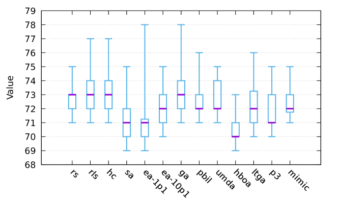
Figure 1: Fixed-budget performance of some search algorithms on the same AOM function ($n=100$, $3\cdot 10^{5}$ evaluations, 20 runs).

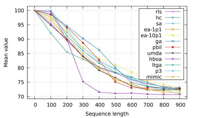
Figure 2: Mean fixed-budget performance of search algorithms on TS-AOM functions as a function of $t\in[0..900]$ ($n=100$, $3\cdot 10^{5}$ evaluations, 20 runs).

Fig. 2 shows the mean fixed-budget performance of search algorithms on TS-AOM functions as a function of sequence length $t\in[0..900]$. For each run, a random TS-AOM function has been generated. The randomness of the performance stems from the random generation of the function and the stochastic behavior of algorithms. This will also be the case for subsequent experiments. For all search algorithms, as $t$ increases, the mean value converges to the mean value observed in the general case (see Fig. 1). This is consistent with the theory of random walks on finite groups [25]. It should be noted that some results [13] only apply to general transvections, as opposed to elementary transvections used in this paper. Finite products of random transvections can be seen as random walks on $\operatorname{GL}(n,\mathbb{F}_{2})$. As $t\rightarrow\infty$, their distributions converge to the uniform distribution on $\operatorname{GL}(n,\mathbb{F}_{2})$. For large $t$, the distribution of random TS-AOM functions is close to the uniform distribution on $\mathcal{F}$, which explains the observed asymptotic behavior. For $t\in[20..200]$, hill climbing is significantly worse than other algorithms. For $t\in[200..300]$, the mean value of HBOA drops faster than that of other algorithms. For $t\in[200..460]$, the genetic algorithm outperforms other algorithms. For $t\in[500..800]$, $(10+1)$ EA outperforms other algorithms.

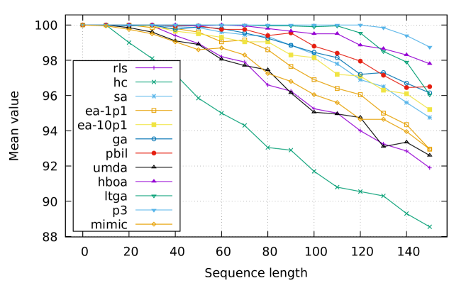
Figure 3: Mean fixed-budget performance of search algorithms on TS-AOM functions as a function of $t\in[0..150]$ ($n=100$, $3\cdot 10^{5}$ evaluations, 20 runs).

In Fig. 3, we turn our attention to TS-AOM functions with small sequence length, that is those not too far from OneMax. The plot shows how search algorithms resist an increasing number of perturbations (elementary transvections). MIMIC is the first algorithm to fail to maximize an instance (at $t=10$) whereas P3 is the last one (at $t=130$).

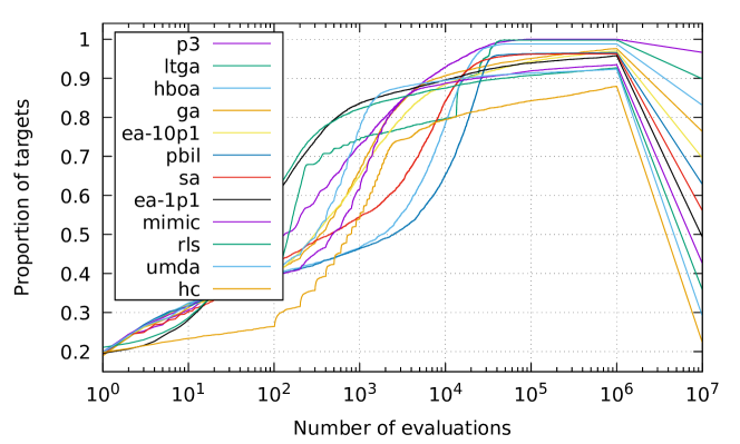
Figure 4: ECDF of search algorithms on 10 TS-AOM functions ($n=100$, $t=100$, $10^{6}$ evaluations, 20 run). Segments on the far right are helper lines to distinguish search algorithms.

Fig. 4 shows the empirical cumulative distribution functions [10] of search algorithms on the same set of 10 TS-AOM functions with $n=100$ and $t=100$.

Fig. 5 shows the mean runtime of $(1+1)$ EA on AOM functions as a function of $n$. The results suggest that the expected runtime of $(1+1)$ EA on AOM functions is exponential in $n$. Fig. 6 shows the mean runtime of $(1+1)$ EA on TS-AOM functions with $n=11$ as a function of $t$. As $t\rightarrow\infty$, the runtime converges to an asymptotic value which is the runtime observed in the general case (see Fig. 5). As already noted, this is consistent with the theory of random walks on finite groups.

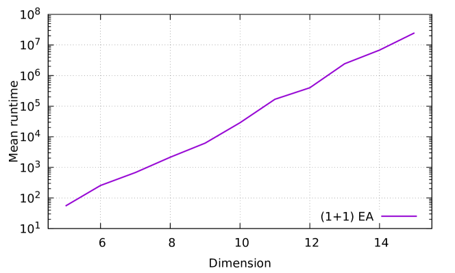
Figure 5: Mean runtime of $(1+1)$ EA on AOM functions as a function of $n$ (50 runs).

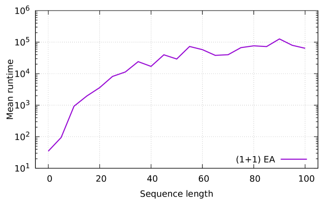
Figure 6: Mean runtime of $(1+1)$ EA on TS-AOM functions as a function of $t$ ($n=11$, 100 runs).

Fig. 7 shows the mean runtime of $(1+1)$ EA on TS-AOM functions with commuting and non commuting transvections and $n=9$ as a function of $t$. By noncommuting transvections we mean that no two consecutive transvections in the sequence commute. We acknowledge that such TS-AOM functions are negligible in the set $\mathcal{F}_{t}\setminus\mathcal{F}_{t}^{c}$. The maximum sequence length is set to $(n^{2}-1)/4=20$, which is the maximum allowed for commuting transvections. Some functions with commuting transvections are significantly harder than others. On the contrary to commuting transvections, the mean and the standard deviation of the runtime with non commuting transvections do not exhibit any peak.

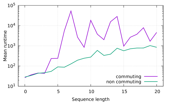
Figure 7: Mean runtime of $(1+1)$ EA on TS-AOM functions with commuting and noncommuting transvections as a function of $t$ ($n=9$, 100 runs).

Fig. 8 shows the mean runtime of $(1+1)$ EA on functions in $\mathcal{F}_{t}^{\delta}$ (unique destination) and $\mathcal{F}_{t}^{\sigma}$ (unique source) with $n=9$ as a function of $t$. The maximum sequence length is set to $n-1=8$, which is the maximum allowed for both $\mathcal{F}_{t}^{\delta}$ and $\mathcal{F}_{t}^{\sigma}$. There is a clear separation between the two classes and $\mathcal{F}_{t}^{\sigma}$ appears to contain the hardest functions.

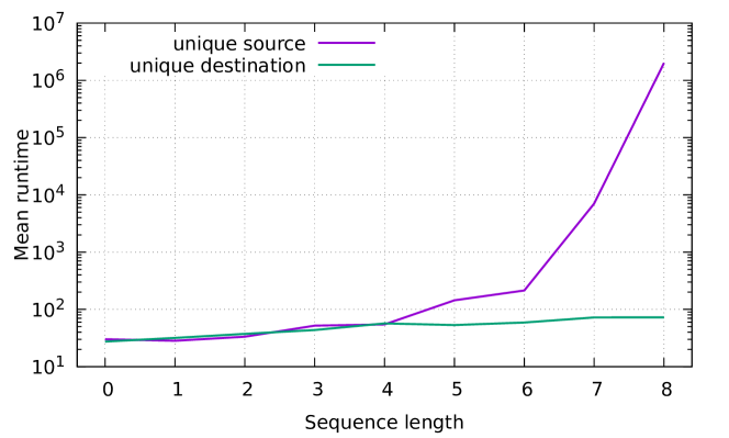
Figure 8: Mean runtime of $(1+1)$ EA on functions in classes $\mathcal{F}_{t}^{\delta}$ (unique destination) and $\mathcal{F}_{t}^{\sigma}$ (unique source) as a function of $t$ ($n=9$, 50 runs).

Fig. 9 shows the mean runtime of $(1+1)$ EA on TS-AOM functions with disjoint transvections and sequence length $\lfloor n/2\rfloor$ as a function of $n$. The results suggest that the expected runtime of $(1+1)$ EA is asymptotically slightly greater on $\mathcal{F}_{\lfloor n/2\rfloor}^{d}$ than on OneMax.

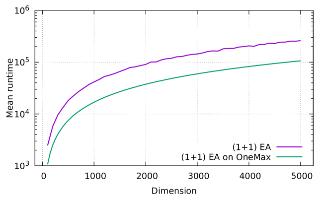
Figure 9: Mean runtime of $(1+1)$ EA on TS-AOM functions with disjoint transvections and sequence length $\lfloor n/2\rfloor$ as a function of $n$ (100 runs).

6 Conclusion

We have introduced affine OneMax functions which are test functions for search algorithms. They are defined as compositions of OneMax and invertible affine maps on bit vectors. They have a simple representation and a known maximum. Tunable complexity is achieved by expressing invertible linear maps as finite products of transvections. The complexity is controlled by the length of transvection sequences and their properties. Transvection sequence AOM functions with small sequence length are of practical interest in the benchmarking of search algorithms. We have shown by means of Fourier analysis that the black box complexity of AOM functions is upper bounded by a high degree polynomial. However, it can be as low as logarithmic for the simplest AOM functions.

Many open questions remain. The gap between the lower and upper bounds of the black box complexity in the general case is significant and should be reduced. A rigorous analysis of the runtime of $(1+1)$ EA on AOM functions would be of great interest. OneMax is one of the simplest nontrivial functions used in black box optimization. It seems legitimate to consider alternative functions to define new classes in the same way as for AOM functions. Candidate functions include pseudo-linear functions or LeadingOnes. However, since LeadingOnes is not sparse, the method presented in this paper does not apply.

References

- [1] Shumeet Baluja and Rich Caruana. Removing the genetics from the standard genetic algorithm. In Armand Prieditis and Stuart Russell, editors, Proc. of the 12th Annual Conf. on Machine Learning, pages 38–46. Morgan Kaufmann, 1995.
- [2] J. S. De Bonet, C. L. Isbell, and P. Viola. MIMIC: finding optima by estimating probability densities. In Advances in Neural Information Processing Systems, volume 9. MIT Press, Denver, 1996.
- [3] Nader H. Bshouty. Optimal algorithms for the coin weighing problem with a spring scale. In Proc. of the 22nd Annual Conf. on Learning Theory (COLT’09), 2009.
- [4] Sung-Soon Choi, Kyomin Jung, and Jeong Kim. Almost tight upper bound for finding fourier coefficients of bounded pseudo-boolean functions. Journal of Computer and System Sciences, 77:123–134, 2008.
- [5] Carola Doerr. Complexity theory for discrete black-box optimization heuristics. In Benjamin Doerr and Frank Neumann, editors, Theory of Evolutionary Computation: Recent Developments in Discrete Optimization, pages 133–212, Cham, 2020. Springer International Publishing.
- [6] Stefan Droste, Thomas Jansen, and Ingo Wegener. Upper and lower bounds for randomized search heuristics in black-box optimization. Theory of Computing Systems, 39(4):525–544, 2006.
- [7] Pál Erdős and Alfréd Rényi. On two problems of information theory. Magyar Tud. Akad. Mat. Kutató Int. Közl, 8:229–243, 1963.
- [8] David E. Goldberg. Genetic algorithms and Walsh functions: Part I, a gentle introduction. Complex systems, 3(2):129–152, 1989.
- [9] Brian W. Goldman and William F. Punch. Fast and efficient black box optimization using the parameter-less population pyramid. Evolutionary Computation, 23(3):451–479, 2015.
- [10] Nikolaus Hansen, Anne Auger, Dimo Brockhoff, Dejan Tusar, and Tea Tusar. COCO: performance assessment. CoRR, abs/1605.03560, 2016.
- [11] Robert B. Heckendorn, Soraya Rana, and Darrell Whitley. Polynomial time summary statistics for a generalization of maxsat. In Proc. of the 1st Annual Conf. on Genetic and Evolutionary Computation, volume 1, pages 281–288, 1999.
- [12] Robert B. Heckendorn, Soraya Rana, and Darrell Whitley. Test function generators as embedded landscapes. In Foundations of Genetic Algorithms, pages 183–198. Morgan Kaufmann, 1999.
- [13] Martin Hildebrand. Generating random elements in by random transvections. Journal of Algebraic Combinatorics, 1(2):133–150, 1992.
- [14] HNCO. https://github.com/courros/hnco. v0.16.
- [15] Wassily Hoeffding. Probability inequalities for sums of bounded random variables. Journal of the American Statistical Association, 58(301):13–30, 1963.
- [16] John H. Holland. Adaptation in natural and artificial systems. University of Michigan Press, Ann Arbor, 1975.
- [17] Stuart A. Kauffman. The origins of order: self-organisation and selection in evolution. Oxford University Press, 1993.
- [18] S. Kirkpatrick, C. D. Gelatt, and M. P. Vecchi. Optimization by simulated annealing. Science, 220(4598):671–680, 1983.
- [19] Eyal Kushilevitz and Yishay Mansour. Learning decision trees using the Fourier spectrum. SIAM Journal on Computing, 22(6):1331–1348, 1993.
- [20] Gunar Liepins and Michael Vose. Representational issues in genetic optimization. J. Exp. Theor. Artif. Intell., 2:101–115, 1990.
- [21] Gunar Liepins and Michael Vose. Polynomials, basis sets, and deceptiveness in genetic algorithms. Complex Systems, 5, 1991.
- [22] Heinz Mühlenbein. The equation for response to selection and its use for prediction. Evolutionary Computation, 5(3):303–346, 1997.
- [23] M. Pelikan and D. Goldberg. Hierarchical bayesian optimization algorithm. In Martin Pelikan, Kumara Sastry, and Erick CantúPaz, editors, Scalable Optimization via Probabilistic Modeling, volume 3 of Studies in Computational Intelligence, pages 63–90. Springer-Verlag Berlin Heidelberg, 2006.
- [24] Sancho Salcedo-Sanz and Carlos Bousoño-Calzón. On the application of linear transformations for genetic algorithms optimization. KES Journal, 11:89–104, 2007.
- [25] Laurent Saloff-Coste. Random walks on finite groups. In Probability on Discrete Structures, pages 263–346. Springer Berlin Heidelberg, 2004.
- [26] Christopher Schumacher, Michael Vose, and Darrell Whitley. The no free lunch and problem description length. In Proc. of the 3rd Annual Conf. on Genetic and Evolutionary Computation (GECCO’01), pages 565–570, San Francisco, CA, USA, 2001. Morgan Kaufmann Publishers Inc.
- [27] Peter F. Stadler. Towards a theory of landscapes. In Complex Systems and Binary Networks, pages 78–163. Springer Berlin Heidelberg, 1995.
- [28] Dirk Thierens. The linkage tree genetic algorithm. In Robert Schaefer, Carlos Cotta, Joanna Kołodziej, and Günter Rudolph, editors, Parallel Problem Solving from Nature, PPSN XI, pages 264–273, Berlin, Heidelberg, 2010. Springer Berlin Heidelberg.