Inverse problem of reconstruction of degenerate diffusion coefficient in a parabolic equation

Abstract

We consider the inverse problem of identification of degenerate diffusion coefficient of the form $x^{\alpha}a(x)$ in a one dimensional parabolic equation by some extra data. We first prove by energy methods the uniqueness and Lipschitz stability results for the identification of a constant coefficient $a$ and the power $\alpha$ by knowing an interior data at some time.

On the other hand, we obtain the uniqueness result for the identification of a general diffusion coefficients $a(x)$ and also the power $\alpha$ form a boundary data on one side of the space interval. The proof is based on global Carleman estimates for a hyperbolic problem and an inversion of the integral transform similar to the Laplace transform. Finally, the theoretical results are satisfactory verified by numerically experiments.

1 Introduction

In this paper we will consider several inverse problems for the following degenerate parabolic equation with two type of degeneracy in the diffusion coefficient. Mainly, weak degeneracy, with $0<\alpha<1$

$$\left\{\begin{array}[]{ll}\partial_{t}u-\partial_{x}(x^{\alpha}a(x)\partial_{x}u)=f(x,t),&(x,t)\in(0,\ell)\times(0,T),\\[2.84526pt] u(0,t)=0,\quad u(\ell,t)=0,&t\in(0,T),\\[2.84526pt] u(x,0)=u_{0}(x),&x\in(0,\ell),\end{array}\right.$$ (1)

and strong degeneracy, with $1\leq\alpha<2$

$$\left\{\begin{array}[]{ll}\partial_{t}u-\partial_{x}(x^{\alpha}a(x)\partial_{x}u)=f(x,t),&(x,t)\in(0,\ell)\times(0,T),\\[2.84526pt] (x^{\alpha}\partial_{x}u(x,t)|_{x=0}=0,\quad u(\ell,t)=0,&t\in(0,T),\\[2.84526pt] u(x,0)=u_{0}(x),&x\in(0,\ell),\end{array}\right.$$ (2)

where $T>0$, $\ell>0$, $u_{0}\in L^{2}(0,\ell)$, $u_{0}\neq 0$, $f\in L^{2}((0,\ell)\times(0,T))$ are given, $a\in C^{1}([0,\ell])$ with $0<\underline{a}\leq a(x)\leq\overline{a}<+\infty$ for all $x\in(0,\ell)$, with $\underline{a}$ and $\overline{a}$ a positive constants.

Our goal is to determine or estimate the diffusion coefficient for the considered degenerate problems. Although we can discuss more general cases, we concentrate here on the one-dimensional linear equation. The following three types of inverse problems of the identification of the unknown diffusion coefficient will be considered and analyzed.

Linear case:

given $\alpha=1$, we will deal with the inverse problem of identification of a constant coefficient, $a(x)\equiv a$, where $a$ is unknown positive constant, form given suitable internal data at some time (see Section 3.1).

Power-like case:

given $a(x)=1$, the inverse problem will be the identification of the power $\alpha\in(0,2)$ from suitable internal observations at some time (see Section 3.2).

General case:

the inverse problem of the identification of a general diffusion coefficient $x^{\alpha}a(x)$ form one boundary observation (see Section 4).

In recent years, degenerate parabolic equations have received increasing attention, in view of the important related theoretical analysis and practical applications, as for example climate science (see Sellers [36], Díaz [12], Huang [24]), populations genetics Ethier [14], vision Citti and Manfredini [9], financial mathematics Black and Scholes [5] and fluid dynamic Oleinik and Samokhin [32]. See also Cannarsa, Martinez and Vancostenoble [7] and references therein.

Inverse problems are the kind of problems known as not well-posed in the sense of Hadamard (see [16]). This means that, either a solution does not exist, or it is not unique and/or small errors in known data lead to large errors in the computation of the solution(s). In particular, the first theoretical issues that we analyze in our paper are uniqueness and stability. The main techniques used here are usual in control and parameter identification theory: tools from real and complex analysis, energy methods and Hardy’s inequality, Laplace and other similar integral transforms, and Carleman inequalities.

The literature related to inverse problems for degenerate parabolic PDEs, despite their fundamental importance and practical applications, is rather recent and scarce. For example, the inverse source problem was considered in Tort [39], Cannarsa, Tort, and Yamamoto [8], Cannarsa, Martinez and Vancostenoble [7], Deng and all [10] and Hussein and all [18], where numerical reconstruction was also considered. The inverse problem of recovering the first-order coefficient of degenerate parabolic equations is analyzed in Deng and Yang [11] and Kamynin [25]. An inverse diffusion problem was considered in [40], where a constant diffusion coefficient was recovered from mesurement of second order derivatives by means of Carleman estimates provided in Cannarsa, Tort and Yamamoto [8].

As for inverse problems of determining spatially varying coefficients such as conductivities and source terms for non-degenerate parabolic equations, we note that there has been a substantial amount of works. Here we are restricted to refer to chapters from Isakov [23], and Yamamoto [41]. See also the references therein. In particular, as for the same type of inverse problems for one-dimensional regular parabolic equations, we refer to Murayama [31], see also Pierce [33], Suzuki and Murayama [37].

On the other hand, most of the techniques that have been developed to treat non-degenerate parabolic equations cease to be applicable in the degenerate case. For instance, for strongly degenerate operators the trace of the co-normal derivate must vanish on the part of the boundary where ellipticity fails, yielding no useful measurement.

The second main issue of this paper is the reconstruction method for our inverse problems. The goal is to compute approximations of the diffusion coefficient as solutions to the inverse problems using the observation data. To our best knowledge, there are no works combining the theoretical studies on the uniqueness, stability and the numerical reconstruction of the diffusion coefficient for a degenerate parabolic equation.

An efficient technique to achieve this, as shown below, relies on a reformulation of the search of the diffusion coefficient as an extremal problem. This is classical nowadays and has been applied in a lot of situations; see for instance Lavrentiev and all  [29], Samarskii and Vabishchevich [35], and Vogel [38].

The paper is organized as follows. In Section 2, we consider the well-posedness of the direct problem (1) and (2). In Section 3.1 we prove, using the energy methods, the Lipschitz stability and the uniqueness result for the linear case corresponding to the constant coefficient $a$. Section 3.2 will be devoted to the power-like case of the identification of the power $\alpha$ in (1) and (2). Again, the Lipschitz stability and the uniqueness will be achieved by the energy methods. In Section 4 a general case of the reconstruction of the unknown general diffusion coefficient $x^{\alpha}a(x)$ will be treated by means of the Carleman estimates, obtaining the uniqueness result for both $\alpha$ and $a(x)$. Finally, in Section 5, in order to illustrate theoretical results obtained in the previous sections, we perform satisfactory numerical experiments corresponding to the considered inverse problems.

2 Preliminaries

In this section we will consider the well-posedness of the direct problem related to (1) and (2). We begin with recalling the natural functions spaces where the problem can be set. For any $\ell>0$, let us call $H=L^{2}(0,\ell)$. For $\alpha\in(0,2)$ we will consider the following function spaces:

$$H_{\alpha}^{1}(0,\ell)=\left\{\begin{array}[]{l}\{u\in H\,|\,\displaystyle\int_{0}^{\ell}x^{\alpha}|\partial_{x}u|^{2}\,dx<\infty,\,u(0)=u(\ell)=0\},\quad 0<\alpha<1,\\[11.38109pt] \{u\in H\,|\,\displaystyle\int_{0}^{\ell}x^{\alpha}|\partial_{x}u|^{2}\,dx<\infty,\,u(\ell)=0\},\quad 1\leq\alpha<2\end{array}\right.$$ (3)

and

$$H_{\alpha}^{2}(0,\ell)=\{u\in H^{1}_{\alpha}(0,\ell)\,|\,x\mapsto x^{\alpha}\partial_{x}u\in H^{1}(0,\ell)\},\quad 0<\alpha<2.$$

Remark 2.1 (Neumann boundary condition)

For $u\in H^{2}_{\alpha}(0,\ell)$ with $1\leq\alpha<2$, we have $x^{\alpha}\partial_{x}u|_{x=0}=0$. Indeed, if $x^{\alpha}\partial_{x}u(x)\to L$ when $x\to 0$, then $x^{\alpha}|\partial_{x}u(x)|^{2}\sim L^{2}/x^{\alpha}$ and, therefore $L=0$ otherwise $u\notin H^{1}_{\alpha}(0,\ell)$.

We now adapt the classical Poincaré inequality to the above weighted spaces.

Lemma 2.2 (Poincare’s inequality)

For all $\varepsilon>0$, there exists a constant $C_{p}=C_{p}(\varepsilon,\ell)>0$ such that for all $\alpha\in[0,2-\varepsilon]$, the following holds:

$$\int_{0}^{\ell}|u|^{2}\,dx\leq C_{p}\int_{0}^{\ell}x^{\alpha}|\partial_{x}u|^{2}\,dx\quad\forall\,u\in H_{\alpha}^{1}(0,\ell).$$ (4)

Proof of Lemma 2.2– Let $\ell>0$ be given. We will distinguish two cases.

1. Assume $\alpha=1$, for all $x\in(0,\ell)$, we have

   $$\begin{array}[]{lll}|u(x)|&\leq&\displaystyle\int_{x}^{\ell}|\partial_{x}u|\,dy\leq\Big{(}\int_{x}^{\ell}y|\partial_{x}u(y)|^{2}\,dy\Big{)}^{1/2}\Big{(}\int_{x}^{\ell}\dfrac{1}{y}\,dy\Big{)}^{1/2}\\[11.38109pt] &\leq&\displaystyle\Big{(}\log\frac{1}{\ell}-\log\dfrac{1}{x}\Big{)}^{1/2}\Big{(}\int_{x}^{\ell}y|\partial_{x}u(y)|^{2}\,dy\Big{)}^{1/2}.\end{array}$$

   Therefore, we obtain

   $$\int_{0}^{\ell}|u(x)|^{2}\,dx\leq\Big{(}\int_{0}^{\ell}\log\dfrac{1}{x}\,dx\Big{)}\int_{0}^{\ell}x|\partial_{x}u(x)|^{2}\,dx=\ell(1-\log\ell)\int_{0}^{\ell}x|\partial_{x}u(x)|^{2}\,dx.$$

2. Assume now that $\alpha\neq 1$. We can write

   $$\begin{array}[]{lll}|u(x)|&\leq&\left|\displaystyle\int_{x}^{\ell}y^{\alpha/2}u^{\prime}(y)\,\dfrac{dy}{y^{\alpha/2}}\right|\leq\left(\displaystyle\int_{x}^{\ell}\dfrac{dy}{y^{\alpha/2}}\right)^{1/2}\displaystyle\left(\int_{0}^{\ell}y^{\alpha}|u^{\prime}(y)|^{2}\,dy\right)^{1/2}\\[11.38109pt] &\leq&\left(\dfrac{\ell^{1-\alpha}-x^{1-\alpha}}{1-\alpha}\right)^{1/2}\displaystyle\left(\int_{0}^{\ell}y^{\alpha}|u^{\prime}(y)|^{2}\,dy\right)^{1/2}\end{array}$$

   Therefore, we obtain

   $$\begin{array}[]{lll}\displaystyle\int_{0}^{\ell}|u(x)|^{2}\,dx&=&\left(\displaystyle\int_{0}^{\ell}\dfrac{\ell^{1-\alpha}-x^{1-\alpha}}{1-\alpha}\,dx\right)\displaystyle\int_{0}^{\ell}x^{\alpha}|\partial_{x}u(x)|^{2}\,dx\\[11.38109pt] &=&\dfrac{\ell^{2-\alpha}}{2-\alpha}\displaystyle\int_{0}^{\ell}x^{\alpha}|\partial_{x}u(x)|^{2}\,dx=C_{p}\displaystyle\int_{0}^{\ell}x^{\alpha}|\partial_{x}u(x)|^{2}\,dx,\end{array}$$

   here we have used that $\alpha<2$. This ends the proof.

   $\square$

For given constants $0<\underline{a}<\overline{a}$, we assume that

$$a\in C^{1}([0,\ell]),\qquad 0<\underline{a}\leq a(x)\leq\overline{a}<+\infty\quad\forall x\in(0,\ell)$$ (5)

Problems (1) and (2) can be recast in the abstract form

$$\begin{cases}u^{\prime}(t)=Au(t)&t\geq 0\vspace{.1cm}\\ u(0)=u_{0}\end{cases}$$ (6)

by introducing the linear operator $A:D(A)\subset H\to H$ defined by

$$D(A)=H_{\alpha}^{2}(0,\ell),\qquad Au=\partial_{x}(x^{\alpha}a(x)\partial_{x}u)\quad\forall u\in D(A).$$ (7)

Observe that the degenerate coefficient $\widetilde{a}(x)=x^{\alpha}a(x)$ is of class $C^{1}([0,\ell])$ and satisfies

$$\lim_{x\to 0}\dfrac{x\widetilde{a}^{\prime}(x)}{\widetilde{a}(x)}=\lim_{x\to 0}\dfrac{x^{\alpha+1}a^{\prime}(x)+\alpha x^{\alpha}a(x)}{x^{\alpha}a(x)}=\alpha\in(0,2).$$ (8)

Therefore, we can appeal to [30] to obtain a well-posedness result for (6) as well as for the nonhomogeneous problem

$$\begin{cases}u^{\prime}(t)=Au(t)+f(t)&t\geq 0\vspace{.1cm}\\ u(0)=u_{0}\end{cases}$$ (9)

So, one can prove the following, where we recall that $D((-A)^{1/2})=H_{\alpha}^{1}(0,\ell)$ for the operator $A$ defined in (7).

Theorem 2.3

Assume (5). Then, $A$ is the infinitesimal generator of a strongly continuous semigroup of contractions, $e^{tA}$. Moreover, $e^{tA}$ is analytic. Therefore, for any $u_{0}\in H$, the solution $u(x,t)=(e^{tA}u_{0})(x)$ of problem (6) satisfies:

• $u\in C([0,\infty);H)$,

• $t\mapsto u(\cdot,t)$ is analytic as a map $(0,+\infty)\longrightarrow H$,

• $u(t)\in\bigcap_{n\geq 1}D(A^{n})$  $\forall\,t>0$.

Furthermore, if $u_{0}\in D((-A)^{1/2})$, then for any $f\in L^{2}(0,T;H)$ the mild solution

$$u(t):=e^{tA}u_{0}+\int_{0}^{t}e^{(t-s)A}f(s)ds\qquad(t\in[0,T])$$

of problem (9) belongs to $H^{1}(0,T;H)\cap C([0,T];D((-A)^{1/2}))\cap L^{2}(0,T;D(A))$ and satisfies the equation in (9) for a.e. $t\in[0,T]$.

Consequently, the equation in (1) and (2) is satisfied in classical sense on $(0,\ell)\times(0,+\infty)$, as well as boundary conditions, taking into account Remark 2.1. As for the initial condition, we recall that $u_{0}\in L^{2}(0,\ell)$ implies that $u\in C^{0}([0,+\infty);L^{2}(0,\ell))$ and $u_{0}\in H^{1}_{\alpha}(0,\ell)$ implies that $u\in C^{0}([0,+\infty);H^{1}_{\alpha}(0,\ell))$. Hereafter, we will assume solutions as smooth as required.

3 Reconstruction by energy methods

3.1 The linear case: uniqueness and Lipschitz stability

Let us consider the linear case in which $a(x)\equiv a$, where $a$ is a constant such that $0<\underline{a}\leq a\leq\overline{a}$ and $\alpha=1$. This corresponds to the problem (2) with strong degeneracy, that is written as follows:

$$\left\{\begin{array}[]{ll}\partial_{t}u-a\,\partial_{x}(x\partial_{x}u)=f(x,t),&x\in(0,\ell),\quad t\in(0,T),\\[2.84526pt] x\,\partial_{x}u(x,t)|_{x=0}=0\quad u(\ell,t)=0,&t\in(0,T),\\[2.84526pt] u(x,0)=u_{0}(x),&x\in(0,\ell).\end{array}\right.$$ (10)

In this section we will analyze the uniqueness and Lipschitz stability for the inverse problem of the identification of the constant coefficient $a$ in (10) from measurements $\partial_{t}u(x,t_{0})$ and $x\partial_{x}u(x,t_{0})$, for some $t_{0}\in(0,T]$ and for all $x\in(0,\ell)$, as is indicated in Theorem 3.1. In Section 5.1 we will perform numerical reconstructions of $a$ related to this inverse problem.

On the other hand, let us note that it is also possible to consider other observations, for example, using the boundary data $\partial_{x}u(\ell,t)$ for all $t\in(0,T)$. The related inverse problem will be the following: given $\eta=\partial_{x}u(\ell,\cdot)$, find $a$ such that the corresponding solution $u^{a}$ of (10) satisfies $\partial_{x}u(\ell,t)=\eta(t)$, for all $t\in(0,T)$. However, uniqueness and stability for this second inverse problem are, to our knowledge, open questions that we will consider in a forthcoming paper. Nonetheless, we have satisfactory numerical approaches for this second inverse problem, that we will present in the Section 5.2.

Let $u_{i}$, $i=1,2$ be the solution of (10) with $a=a_{i}$, that is to say

$$\left\{\begin{array}[]{ll}\partial_{t}u_{i}-a_{i}\,\partial_{x}(x\partial_{x}u_{i})=f(x,t),&x\in(0,\ell),\quad t\in(0,T),\\[2.84526pt] x\,\partial_{x}u_{i}(x,t)|_{x=0}=0\quad u_{i}(\ell,t)=0,&t\in(0,T),\\[2.84526pt] u_{i}(x,0)=u_{0}(x),&x\in(0,\ell).\end{array}\right.$$ (11)

The main result of this section is the following:

Theorem 3.1

Assume that $a_{1},\,a_{2}\in C^{1}([0,\ell])$, $0<\underline{a}\leq a_{1},a_{2}\leq\overline{a}<+\infty$ for all $x\in(0,\ell)$, $u_{0}\in L^{2}(0,\ell)$, $u_{0}\neq 0$ and $f\in L^{2}((0,\ell)\times(0,T))$. Let $u_{1},u_{2}$ be solutions of (11) satisfying the following hypothesis: for some $t_{0}\in(0,T]$ and $\mu>0$ such that

$$\int_{0}^{\ell}x|\partial_{x}u_{i}(x,t_{0})|^{2}\,dx\geq\mu,\quad i=1,2.$$ (12)

Then there exists a positive constant $C=C(\underline{a},\mu)$ such that

$$|a_{2}-a_{1}|\leq C\left(\int_{0}^{\ell}\big{(}|\partial_{t}u_{1}(x,t_{0})-\partial_{t}u_{2}(x,t_{0})|^{2}+x|\partial_{x}u_{2}(x,t_{0})-\partial_{x}u_{1}(x,t_{0})|^{2}\big{)}\,dx\right)^{1/2}.$$ (13)

Remark 3.2

Notice that, as we have mentioned before, we can obtain similar uniqueness result for more general equations containing zero order therms.

Remark 3.3

Recall that, since $e^{tA}$ is analytic, $u_{i}(t,\cdot)\in H_{1}^{2}(0,\ell)$ for a.e. $t>0$, $i=1,2$. Moreover, assuming in addition that $f\equiv 0$, we have the following.

1. By backward uniqueness we know that, if $u_{0}\neq 0$, then the solution $u$ of (10) satisfies

   $$\int_{0}^{\ell}x|\partial_{x}u(x,t)|^{2}\,dx>0\quad\forall\,t\in[0,T].$$ (14)

   This explains the role played by assumption (12) above.

2. Since $A$ is dissipative, we have that

   $$\int_{0}^{\ell}x|\partial_{x}u_{i}(x,t)|^{2}\,dx\geq\int_{0}^{\ell}x|\partial_{x}u_{i}(x,T)|^{2}\,dx\quad\forall\,t\in[0,T].$$

   Therefore,

   $$\mu=\min_{i=1,2}\displaystyle\int_{0}^{\ell}x|\partial_{x}u_{i}(x,T)|^{2}\,dx$$

   is a possible choice of $\mu$ for every $t_{0}\in(0,T]$.

3. Another way to construct $\mu>0$ satisfying (12) is to take $u_{0}\in D(A)$, observing that

   $$\int_{0}^{\ell}x|\partial_{x}u(t,x)|^{2}\,dx\geq\displaystyle\int_{0}^{\ell}x|\partial_{x}u_{0}(x)|^{2}\,dx-2t\displaystyle\int_{0}^{\ell}|(x\partial_{x}u_{0})_{x}|^{2}\,dx.$$

   Therefore, (12) holds with $\mu=\dfrac{1}{2}\displaystyle\int_{0}^{\ell}x|\partial_{x}u_{0}(x)|^{2}\,dx$ for all

   $$0<t_{0}<\dfrac{1}{4}\,\dfrac{\displaystyle\int_{0}^{\ell}x|\partial_{x}u_{0}(x)|^{2}\,dx}{\displaystyle\int_{0}^{\ell}|(x\partial_{x}u_{0})_{x}|^{2}\,dx}\,.$$

Proof of Theorem 3.1 – We assume that $a_{2}\geq a_{1}$ and set $w=u_{1}-u_{2}$. Then, we can write

$$\partial_{t}w-a_{1}\,\partial_{x}(x\partial_{x}w)=(a_{1}-a_{2})\partial_{x}(x\partial_{x}u_{2}).$$

Multiplying by $u_{2}$ and integrating by parts this equality, we get

$$\begin{array}[]{l}\displaystyle(a_{2}-a_{1})\int_{0}^{\ell}x|\partial_{x}u_{2}|^{2}\,dx=\displaystyle\int_{0}^{\ell}u_{2}\partial_{t}w\,dx+a_{1}\int_{0}^{\ell}x\partial_{x}w\partial_{x}u_{2}\,dx\\[11.38109pt] \leq\displaystyle\left(\int_{0}^{\ell}|u_{2}|^{2}\,dx\right)^{1/2}\left(\int_{0}^{1}|\partial_{t}w|^{2}\,dx\right)^{1/2}+a_{1}\left(\int_{0}^{\ell}x|\partial_{x}w|^{2}\,dx\right)^{1/2}\left(\int_{0}^{\ell}x|\partial_{x}u_{2}|^{2}\,dx\right)^{1/2}.\end{array}$$

So, by (4), we have

$$\begin{array}[]{l}\displaystyle|a_{2}-a_{1}|\int_{0}^{\ell}x|\partial_{x}u_{2}|^{2}\,dx\\[11.38109pt] \leq\displaystyle\left(\sqrt{C_{p}}\left(\int_{0}^{\ell}|\partial_{t}w|^{2}\,dx\right)^{1/2}+a_{1}\left(\int_{0}^{\ell}x|\partial_{x}w|^{2}\,dx\right)^{1/2}\right)\left(\int_{0}^{\ell}x|\partial_{x}u_{2}|^{2}\,dx\right)^{1/2},\end{array}$$ (15)

which in turn yields the the conclusion in view of (12) and ends the proof of this theorem. $\square$

It is clear that from the proof of this theorem we can deduce the following uniqueness result.

Corollary 3.4

Let us assume that $a_{1},\,a_{2}\geq\underline{a}>0$, $f\equiv 0$, and $u_{0}\in L^{2}(0,\ell)$, $u_{0}\neq 0$. If $u_{1},u_{2}\in C^{0}([0,T];L^{2}(0,\ell))$ are solutions of (11) such that for some $t_{0}\in(0,T]$ we have $\partial_{t}u_{1}(x,t_{0})=\partial_{t}u_{2}(x,t_{0})$ and $\partial_{x}u_{2}(x,t_{0})=\partial_{x}u_{1}(x,t_{0})$ for all $x\in(0,\ell)$, then $a_{1}=a_{2}$.

Indeed, it is enough to realize that we do not need hypothesis (12) for uniqueness, because we do not need the constant in (15) to be uniform. Therefore, form (15) and thanks to the inequality (14), we obtain uniqueness.

3.2 The power-like case: uniqueness and Lipschitz stability

In this section we will consider the inverse problem of identification of the power $\alpha$ in the degenerate parabolic problems (1) and (2), assuming for simplicity that $a(x)\equiv 1$ and $f\equiv 0$. That is to say, that we will consider the following problems: with weak degeneracy $(0\leq\alpha<1)$

$$\left\{\begin{array}[]{ll}\partial_{t}u-\partial_{x}(x^{\alpha}\partial_{x}u)=0,&(x,t)\in(0,\ell)\times(0,T),\\[2.84526pt] u(0,t)=0,\quad u(\ell,t)=0,&t\in(0,T),\\[2.84526pt] u(x,0)=u_{0}(x),&x\in(0,\ell)\end{array}\right.$$ (16)

and with strong degeneracy $(1\leq\alpha<2)$

$$\left\{\begin{array}[]{ll}\partial_{t}u-\partial_{x}(x^{\alpha}\partial_{x}u)=0,&(x,t)\in(0,\ell)\times(0,T),\\[2.84526pt] x^{\alpha}\partial_{x}u(x,t)|_{x=0}=0,\quad u(\ell,t)=0,&t\in(0,T),\\[2.84526pt] u(x,0)=u_{0}(x),&x\in(0,\ell).\end{array}\right.$$ (17)

Similarly to what we have done in the Section 3.1, we will analyze uniqueness and stability for the inverse problem of identification of the power $\alpha$ in the above problems from measurements $\partial_{t}u(x,t_{0})$ and $x\partial_{x}u(x,t_{0})$, for some $t_{0}\in(0,T]$ and for all $x\in(0,\ell)$. In Section 5.3 we will perform the numerical reconstruction of $\alpha$ for the problems (16) and (17).

As we have noted in the previous section, is also possible to consider the inverse problem of identification of the power $\alpha$ with only one boundary observation, for example $\partial_{x}u(\ell,t)$ for all $t\in(0,T)$. However, the uniqueness and stability related to this second inverse problem is, to our knowledge, an open questions. Nevertheless, we have satisfactory numerical approaches for this second inverse problem, that we will expose in the Section 5.4.

In this section, we analyze uniqueness and stability for the power $\alpha$ in (17) and (16). Let us start with a uniqueness result.

Theorem 3.5

Let assume that $0<\ell\leq 1$, $u_{0}\in L^{2}(0,\ell)$, $u_{0}\neq 0$ and $u_{i}$, $i=1,2$, be the solution of (17) (or (16)) corresponding to $\alpha_{i}$ such that for some $t_{0}\in(0,T]$ we have $\partial_{t}u_{1}(x,t_{0})=\partial_{t}u_{2}(x,t_{0})$ and $\partial_{x}u_{1}(x,t_{0})=\partial_{x}u_{2}(x,t_{0})$ for all $x\in(0,\ell)$, then $\alpha_{1}=\alpha_{2}$.

Proof of Theorem – We can assume, without loss of generality, that $\alpha_{1}<\alpha_{2}$. Setting

$$w(x,t)=u_{2}(x,t)-u_{1}(x,t),$$

we have

$$\partial_{t}w-\partial_{x}(x^{\alpha_{2}}\partial_{x}w)=\partial_{x}((x^{\alpha_{2}}-x^{\alpha_{1}})\partial_{x}u_{1}).$$ (18)

Then, multiplying this equality by $u_{1}$ and integrating by parts, we obtain

$$\int_{0}^{\ell}(x^{\alpha_{1}}-x^{\alpha_{2}})|\partial_{x}u_{1}|^{2}\,dx=\int_{0}^{\ell}(u_{1}\partial_{t}w+x^{\alpha_{2}}\partial_{x}w\,\partial_{x}u_{1})\,dx.$$ (19)

By hypothesis, we have that there exists $t_{0}\in(0,T]$ such that $\partial_{t}w(\cdot,t_{0})=\partial_{x}w(\cdot,t_{0})=0$. Then, from (19) we have

$$\int_{0}^{\ell}(x^{\alpha_{1}}-x^{\alpha_{2}})|\partial_{x}u_{1}(t_{0},x)|^{2}\,dx\leq 0.$$

Since $x^{\alpha_{1}}>x^{\alpha_{2}}$ for all $x\in(0,\ell)$, the above inequality yields

$$\partial_{x}u_{1}(\cdot,t_{0})=0\quad\text{a.e. on }(0,\ell).$$

By backward uniqueness, this implies that $u_{0}=0$ which is excluded by the hypothesis. This ends the proof. $\square$

Remark 3.6

In the above uniqueness result, the observability assumption $\partial_{x}u_{1}(\cdot,t_{0})=\partial_{x}u_{2}(\cdot,t_{0})$ can be replaced by $u_{1}(\cdot,t_{0})=u_{2}(\cdot,t_{0})$.

Theorem 3.7 (Lipschitz stability)

Let us assume that $0<\ell<1$, $0\leq\alpha_{1},\alpha_{2}\leq 2-\varepsilon$, for some $\varepsilon\in(0,2)$, and $u_{0}\in L^{2}(0,\ell)$, $u_{0}\neq 0$. Let $u_{1}$ and $u_{2}$ be the solutions of (17) (or (16)), corresponding to $\alpha_{i}(i=1,2)$, satisfying the following hypothesis: for some $t_{0}\in(0,T]$ and $\mu>0$

$$\int_{0}^{\ell}x^{\alpha_{i}}|\partial_{x}u_{i}(x,t_{0})|^{2}\,dx>\mu.$$ (20)

Then there exists a constant $C=C(\varepsilon,\ell)>0$ such that

$$|\alpha_{2}-\alpha_{1}|\leq C\left(\int_{0}^{\ell}\Big{(}|\partial_{t}(u_{1}(x,t_{0})-u_{2}(x,t_{0}))|^{2}+x^{\alpha_{1}\vee\alpha_{2}}|\partial_{x}(u_{1}(x,t_{0})-u_{2}(x,t_{0}))|^{2}\Big{)}\,dx\right)^{1/2},$$ (21)

where $\alpha_{1}\vee\alpha_{2}=\max\{\alpha_{1},\alpha_{2}\}$.

Remark 3.8

The hypothesis $0<\ell<1$ in the Theorem 3.7 is essential in the proof.

Proof of Theorem 3.7 – We assume, without loss of generality, that $\alpha_{1}<\alpha_{2}$. We notice that for $0\leq\alpha_{1}<\alpha_{2}$, we have $H_{\alpha_{1}}^{1}(0,\ell)\hookrightarrow H^{1}_{\alpha_{2}}(0,\ell)$, where the spaces $H^{1}_{\alpha_{i}}(0,\ell)$ are given by (3).

As before, setting

$$w(x,t)=u_{2}(x,t)-u_{1}(x,t),$$

we have (18) and (19). Now, we observe that

$$\int_{0}^{\ell}(x^{\alpha_{1}}-x^{\alpha_{2}})|\partial_{x}u_{1}|^{2}\,dx=\int_{0}^{\ell}(1-x^{\alpha_{2}-\alpha_{1}})x^{\alpha_{1}}|\partial_{x}u_{1}|^{2}\,dx\geq(1-\ell^{\alpha_{2}-\alpha_{1}})\int_{0}^{\ell}x^{\alpha_{1}}|\partial_{x}u_{1}|^{2}\,dx.$$

On the other hand, we have

$$1-\ell^{\alpha_{2}-\alpha_{1}}=\displaystyle\int_{\ell}^{1}\dfrac{d}{d\lambda}\lambda^{\alpha_{2}-\alpha_{1}}\,d\lambda=(\alpha_{2}-\alpha_{1})\displaystyle\int_{\ell}^{1}\lambda^{\alpha_{2}-\alpha_{1}-1}\,d\lambda\geq(\alpha_{2}-\alpha_{1})\ell(1-\ell).$$ (22)

Here, we have used that

$$\int_{\ell}^{1}\lambda^{\alpha_{2}-\alpha_{1}-1}\,d\lambda\geq\ell(1-\ell),$$

since if $\alpha_{2}-\alpha_{1}-1\leq 0$, we have $\lambda^{\alpha_{2}-\alpha_{1}-1}\geq 1>\ell$ and if $0<\alpha_{2}-\alpha_{1}-1<1$, we have $\lambda^{\alpha_{2}-\alpha_{1}-1}\geq\ell^{\alpha_{2}-\alpha_{1}-1}>\ell$.

Therefore, we conclude that

$$(\alpha_{2}-\alpha_{1})\ell(1-\ell)\displaystyle\int_{0}^{\ell}x^{\alpha_{1}}|\partial_{x}u_{1}|^{2}\,dx\leq\displaystyle\int_{0}^{\ell}(x^{\alpha_{1}}-x^{\alpha_{2}})|\partial_{x}u_{1}|^{2}\,dx.$$ (23)

Next, by Poincare’s inequality (4), for the right-hand side of (19) we have that

$$\begin{array}[]{l}\displaystyle\int_{0}^{\ell}(u_{1}\partial_{t}w+x^{\alpha_{2}}\partial_{x}w\,\partial_{x}u_{1})\,dx\\[11.38109pt] \leq\left(\displaystyle\int_{0}^{\ell}|u_{1}|^{2}\,dx\right)^{1/2}\left(\displaystyle\int_{0}^{\ell}|\partial_{t}w|^{2}\,dx\right)^{1/2}\\[11.38109pt] \phantom{+}+\left(\displaystyle\int_{0}^{\ell}x^{\alpha_{2}}|\partial_{x}u_{1}|^{2}\,dx\right)^{1/2}\left(\displaystyle\int_{0}^{\ell}x^{\alpha_{2}}|\partial_{x}w|^{2}\,dx\right)^{1/2}\\[11.38109pt] \leq\sqrt{C_{p}}\left(\displaystyle\int_{0}^{\ell}x^{\alpha_{1}}|\partial_{x}u_{1}|^{2}\,dx\right)^{1/2}\left(\displaystyle\int_{0}^{\ell}|\partial_{t}w|^{2}\,dx\right)^{1/2}\\[11.38109pt] \phantom{+}+\ell^{(\alpha_{2}-\alpha_{1})/2}\left(\displaystyle\int_{0}^{\ell}x^{\alpha_{1}}|\partial_{x}u_{1}|^{2}\,dx\right)^{1/2}\left(\displaystyle\int_{0}^{\ell}x^{\alpha_{2}}|\partial_{x}w|^{2}\,dx\right)^{1/2}.\end{array}$$ (24)

The conclusion follows from (23) and (24). This ends the proof. $\square$

4 Reconstruction by Carleman inequalities: a general case

We consider now the identification of a spatially varying diffusion coefficient $x^{\alpha}a(x)$ in a degenerate parabolic equation (1):

$$\left\{\begin{array}[]{ll}\partial_{t}u-\partial_{x}(x^{\alpha}a(x)\partial_{x}u)=0,&(x,t)\in(0,1)\times(0,T),\\[2.84526pt] u(0,t)=0,\quad u(1,t)=0,&t\in(0,T),\\[2.84526pt] u(x,0)=u_{0}(x),&x\in(0,1),\end{array}\right.$$ (25)

where we take $\ell=1$ for simplicity. We assume

$$0<\alpha<1,$$

which corresponds to the weak degeneracy. We can discuss also the case $1<\alpha<2$ but we postpone for keeping the article concise.

For suitably given initial value $u_{0}$ and coefficient $a$ which are stated below, there exists a unique solution to (25) by Theorem 2.3 in Section 2 and by $u_{a,\alpha}$, we denote the solution.

The inverse problem that we will consider in this section is to recover $a(x)$, $0<x<1$ and $\alpha\in(0,1)$ from the boundary measurements $\partial_{x}u_{a,\alpha}(1,t)$, provided that unknown $a$ and initial value $u_{0}$ belong to some admissible sets introduced below.

4.1 Uniqueness result

Henceforth, we denote by ^′ the derivative with respect to one single variable, for example, $u^{\prime}_{0}(x)=\frac{du_{0}}{dx}$, $\eta^{\prime}(t)=\frac{d\eta}{dt}$,…, since there is no fear of confusion.

For statement of our main results on the uniqueness in determining diffusion coefficients, we need to introduce admissible sets where unknown coefficients vary. Moreover, we need some regularity for the solutions to (25), which requires compatibility conditions involving unknown coefficients and initial values. Thus the descriptions of the admissible sets are concerned with both coefficients and initial values.

First we set $W^{1,1}(0,T):=\{a\in L^{1}(0,T);\,a^{\prime}\in L^{1}(0,T)\}$ and

$$\mathcal{A}_{0}:=\{(a,\alpha,u_{0})\in C^{3}([0,1])\times(0,1)\times C^{4}([0,1]);\,\,u_{0},\,(x^{\alpha}a(x)u_{0}^{\prime})^{\prime}\in W^{1,1}(0,1),$$

$$(x^{\alpha}a(x))^{1/2}u_{0}^{\prime},\,\,(x^{\alpha}a(x))^{1/2}(x^{\alpha}a(x)u_{0}^{\prime})^{\prime\prime}\in L^{2}(0,1),\,\,x^{\alpha}a(x)u_{0}^{\prime}\in H^{1}(0,1),$$

$$x^{\alpha}a(x)(x^{\alpha}a(x)u_{0}^{\prime})^{\prime\prime}\in H^{1}(0,1),$$

$$u_{0}(\xi)=0,\quad(x^{\alpha}au_{0}^{\prime})^{\prime}(\xi)=0\quad\mbox{for $\xi=0,\,1$}\}.$$ (26)

Remark 4.1

We assume $(a,\alpha,u_{0})\in\mathcal{A}_{0}$ in order to conclude the regularity for $\widetilde{u}_{a,\alpha}$ that we will introduce in Lemma 4.5.

We arbitrarily fix constants $\delta_{0}>0$, $\delta_{1}>0$, $\varepsilon_{0}>0$, $\varepsilon_{1}>0$, and a function $a_{0}\in C^{2}([0,1])$ satisfying $a_{0}>0$ on $[0,1]$. In terms of $\mathcal{A}_{0}$, we define an admissible set of coefficients $x^{\alpha}a(x)$ and initial values $u_{0}(x)$:

$$\begin{array}[]{ll}\mathcal{A}(\varepsilon_{0},\varepsilon_{1},\delta_{0},\delta_{1}):=&\{(a,\alpha,u_{0})\in\mathcal{A}_{0}:\,a\geq\delta_{0}\text{ on }[0,1],\,a(x)=a_{0}(x)\mbox{ for $1-\varepsilon_{0}\leq x\leq 1$},\\[5.69054pt] &|u_{0}^{\prime}(x)|\geq\delta_{1}\text{ for }\varepsilon_{1}\leq x\leq 1\}.\end{array}$$ (27)

By $a=a_{0}$ on $[1-\varepsilon_{0},1]$, we notice that the non-degenerate component $a(x)$ of a diffusion coefficient is assumed to be given near $x=1$, and our concerns is the determination in an interior interval inside $(0,1)$.

The main uniqueness result for the inverse problem of determining a diffusion coefficient $x^{\alpha}a(x)$ is the following:

Theorem 4.2

Let $u_{a,\alpha}$ and $u_{b,\beta}$ be the solutions of (25) corresponding to $(a,\alpha,u_{0})$, $(b,\beta,u_{0})\in\mathcal{A}(\varepsilon_{0},\varepsilon_{1},\delta_{0},\delta_{1})$, respectively. If

$$\partial_{x}u_{a,\alpha}(1,t)=\partial_{x}u_{b,\beta}(1,t),\quad 0<t<t_{0},$$ (28)

with some $t_{0}>0$, then

$$x^{\alpha}a(x)=x^{\beta}b(x),\quad\varepsilon_{1}\leq x\leq 1.$$

The constant $t_{0}>0$ can be chosen independently of $\varepsilon_{0},\varepsilon_{1},\delta_{0}$ and $\delta_{1}$.

The theorem asserts the uniqueness in determining of $x^{\alpha}a(x)$ for $\varepsilon_{1}\leq x\leq 1$ within an admissible set $\mathcal{A}(\varepsilon_{0},\varepsilon_{1},\delta_{0},\delta_{1})$ of coefficients and initial value.

The characterization of the admissible set $\mathcal{A}(\varepsilon_{0},\varepsilon_{1},\delta_{0},\delta_{1})$ is not given separately for $x^{\alpha}a(x)$ and $u_{0}(x)$. However, we can provide a subset of it as follows. We arbitrarily fix $u_{0}\in C^{4}([0,1])$ and positive constants $\varepsilon_{1},\varepsilon_{2},\delta_{1}$ such that

$$u_{0}(x)=0\quad\mbox{for $0\leq x\leq\varepsilon_{2}$},\qquad|u_{0}^{\prime}(x)|\geq\delta_{1}\quad\mbox{for $\varepsilon_{1}\leq x\leq 1$},\quad u_{0}(1)=u_{0}^{\prime\prime}(1)=0.$$ (29)

Whenever $0<\alpha<1$ and a function $a$ satisfies

$$\left\{\begin{array}[]{rl}&a\in C^{3}([0,1]),\quad a\geq\delta_{0}\text{ on }[0,1],\quad a(x)=a_{0}(x)\quad\mbox{for $1-\varepsilon_{0}\leq x\leq 1$},\\[5.69054pt] &(x^{\alpha}a)^{\prime}(1)=\alpha a(1)+a^{\prime}(1)=0,\end{array}\right.$$ (30)

we see that $(a,\alpha,u_{0})\in\mathcal{A}(\varepsilon_{0},\varepsilon_{1},\delta_{0},\delta_{1})$. Thus, (30) is a description of an admissible set of unknown coefficients, which is written independently of $u_{0}$.

Corollary 4.3

Let $u_{0}$ satisfy (29). If $(a,\alpha)$ and $(b,\beta)$ satisfy (30) and

$$\partial_{x}u_{a,\alpha}(1,t)=\partial_{x}u_{b,\beta}(1,t),\quad 0<t<t_{0}$$

with some $t_{0}>0$, then

$$x^{\alpha}a(x)=x^{\beta}b(x),\quad\varepsilon_{1}\leq x\leq 1.$$

In Theorem 4.2, we cannot identify the non-degenerate component $a(x)$ separately from the degeneracy power $\alpha$. However, under a stricter condition on an initial value $u_{0}$, we can uniquely determine both $a(x)$ and $\alpha$. More precisely, we define another admissible set $\mathcal{A}_{1}(\varepsilon_{0},\delta_{0})$ as a subset of $\mathcal{A}(\varepsilon_{0},\varepsilon_{1},\delta_{0},\delta_{1})$ by

$$\begin{array}[]{ll}\mathcal{A}_{1}(\varepsilon_{0},\delta_{0}):=&\{(a,\alpha,u_{0})\in\mathcal{A}_{0};\,a\geq\delta_{0}\text{ on }[0,1],\\[5.69054pt] &a(x)=a_{0}(x)\quad\mbox{for $1-\varepsilon_{0}\leq x\leq 1$},\quad|u_{0}^{\prime}(x)|>0\quad\text{for $0<x\leq 1$}\}.\end{array}$$ (31)

We can write

$$\mathcal{A}_{1}(\varepsilon_{0},\delta_{0})=\bigcap_{\varepsilon_{1}>0,\delta_{1}>0}\mathcal{A}(\varepsilon_{0},\varepsilon_{1},\delta_{0},\delta_{1}).$$

Then we have

Theorem 4.4

Assume that $u_{a,\alpha}$ and $u_{b,\beta}$ be the solutions of (25) corresponding to $(a,\alpha,u_{0})$, $(b,\beta,u_{0})\in\mathcal{A}_{1}(\varepsilon_{0},\delta_{0})$, respectively. If

$$\partial_{x}u_{a,\alpha}(1,t)=\partial_{x}u_{b,\beta}(1,t),\quad 0<t<t_{0},$$

with some $t_{0}\in(0,T)$, then

$$a(x)=b(x),\quad 0\leq x\leq 1\quad\text{and}\quad\alpha=\beta.$$

Proof of Theorem 4.4. The proof of Theorem 4.4 follows directly from Theorem 4.2. Indeed, let $(a,\alpha,u_{0}),(b,\beta,u_{0})\in\mathcal{A}_{1}(\varepsilon_{0},\delta_{0})$. Then, for any $\varepsilon_{1}>0$, we can choose $\delta_{1}>0$ such that $|u_{0}(x)|\geq\delta_{1}$ for $\varepsilon_{1}\leq x\leq 1$. Therefore, applying Theorem 4.2, we see that $x^{\alpha}a(x)=x^{\beta}b(x)$ for $\varepsilon_{1}\leq x\leq 1$. Here we notice that in Theorem 4.2 the constant $t_{0}>0$ is independent of $\varepsilon_{1}$ and $\delta_{1}$.

Since $\varepsilon_{1}>0$ is arbitrary and $a,b\in C([0,1])$, we obtain

$$x^{\alpha}a(x)=x^{\beta}b(x),\quad 0\leq x\leq 1.$$

Assume $\alpha>\beta$. Then $x^{\alpha-\beta}a(x)=b(x)$ for $0<x\leq 1$. Letting $x\downarrow 0$, we reach $b(0)=0$. This contradicts $b(0)\geq\delta_{0}>0$. Similarly, $\alpha<\beta$ is impossible. Hence $\alpha=\beta$, and so $a(x)=b(x)$ for $0\leq x\leq 1$. Thus Theorem 4.4 is proved. $\square$.

Our proof of Theorem 4.2 is based on Carleman estimates, and the methodology requires some positivity related to the initial value, and in our case, $|u_{0}^{\prime}(x)|$ must be positive in the interval $[\varepsilon_{1},1]$ where we want to determine coefficients. It may be practical that we formulate an inverse problem with the zero initial condition and some non-zero boundary condition. However, in that case, our proof does not work.

As is described in Section 4.2.1, the proof of Theorem 4.2 is involved with an inversion of the integral transform which is similar to the Laplace transform. Therefore, the stability rate is expected to be a quite weak, although we can try to consider stability for our inverse problem which should be conditional under some a priori boundedness condition.

On the other hand, we can consider an inverse problem for the system where $u(x,0)=u_{0}(x)$, $x\in(0,1)$ in (25) is replaced by $u(x,t_{0})=u_{0}(x)$, $x\in(0,1)$ with fixed $t_{0}>0$. In this case, we can prove conditional stability of Lipschitz or Hölder type (see Imanuvilov and Yamamoto [20], and Yamamoto [41]). We remark that in Theorem 4.2 the inverse problem corresponds to the classical initial boundary value problem.

4.2 Proof of Theorem 4.2

This section is devoted to the proof of Theorem 4.2. The proof is based on Carleman estimate and such a methodology can be found in Bukhgeim and Klibanov [6], and then Bellassoued and Yamamoto [4], Huang, Imanuvilov and Yamamoto [17], Imanuvilov and Yamamoto [20], [21], [22], and Klibanov [26]. However, the methodology itself for a parabolic equation needs data $u(\cdot,t_{0})$ at $t_{0}>0$, not $u(\cdot,0)$ for a parabolic type of equations. Therefore, we first transform our inverse problem for parabolic equation to an inverse hyperbolic problem by an integral transform in $t$ and then we establish the uniqueness for the transformed inverse hyperbolic problem. Thus, the proof of Theorem 4.2 is divided into the following three steps.

Section 4.2.1: First Step. We transform the inverse parabolic problem to an inverse hyperbolic problem.

Section 4.2.2: Second Step. We apply the method from [6] to a linearized inverse hyperbolic problem and establish the uniqueness. For a general coefficient $a(x)>0$ of the principal term, a key Carleman estimate can be proved locally only in $x$, and we have to argue starting at $x=1$ and we can prove the uniqueness in a small $x$-interval. Then, we repeat the argument for the uniqueness until the $x$-interval of the uniqueness can reach $x=\varepsilon_{1}$.

Section 4.2.3: Thirds Step. We translate the uniqueness for the linearized inverse hyperbolic problem to the original inverse parabolic problem and complete the proof of Theorem 4.2.

4.2.1 First Step: Reduction to hyperbolic problem

We introduce an integral transform called the Reznitskaya transform, and we prove Lemma 4.8 which connects the inverse parabolic problem to an inverse hyperbolic problem. For this transform, we can refer to Romanov [34]. Notice that Klibanov [26], pp. 594-595 have used the transform to prove the uniqueness for an inverse problem for non-degenerate parabolic equations. In our article, the regularity of the solution to (25) requires careful justification in applying the transform, which is made through Lemmas 4.5-4.7.

Let us first consider a system of the second order in $t$. More precisely, let $\widetilde{u}_{a,\alpha}=\widetilde{u}_{a,\alpha}(x,t)$ satisfy

$$\left\{\begin{array}[]{ll}\partial_{t}^{2}\widetilde{u}_{a,\alpha}=\partial_{x}(x^{\alpha}a(x)\partial_{x}\widetilde{u}_{a,\alpha}),&0<x<1,\quad t>0,\\[5.69054pt] \widetilde{u}_{a,\alpha}(0,t)=\widetilde{u}_{a,\alpha}(1,t)=0,&t>0,\\[5.69054pt] \widetilde{u}_{a,\alpha}(x,0)=u_{0}(x),\quad\partial_{t}\widetilde{u}_{a,\alpha}(x,0)=0,&0<x<1.\end{array}\right.$$ (32)

In view of (29) and (30), by Alabau-Boussouira, Cannarsa and Leugering [1], we can prove the following result.

Lemma 4.5

Let $(a,\alpha,u_{0})\in\mathcal{A}(\varepsilon_{0},\varepsilon_{1},\delta_{0},\delta_{1})$, $\mu\in(0,1)$ and $T>0$ be arbitrary. There exists a unique solution to (32) such that

$$\widetilde{u}_{a,\alpha}\in C^{3}([0,\infty);H^{1}(\mu,1))\cap C^{2}([0,\infty);H^{2}(\mu,1))\cap C^{1}([0,\infty);H^{3}(\mu,1))$$ (33)

and

$$\partial_{t}\partial_{x}^{2}\widetilde{u}_{a,\alpha}\in L^{\infty}((\mu,1)\times(0,T)).$$ (34)

Moreover, the following regularity properties hold:

$$\partial_{t}^{2}\widetilde{u}_{a,\alpha}\in L^{\infty}(0,\infty;L^{2}(\mu,1)),\quad\partial_{t}\widetilde{u}_{a,\alpha}\in L^{\infty}(0,\infty;H^{1}(\mu,1)),\quad\widetilde{u}_{a,\alpha}\in L^{\infty}(0,\infty;H^{2}(\mu,1))$$ (35)

and for arbitrarily given $M>0$, there exists a constant $C=C(M,\mu,T)>0$ such that

$$\|\partial_{t}\partial_{x}^{2}\widetilde{u}_{a,\alpha}\|_{L^{\infty}(\mu,1)\times(0,T))} +\sum_{k,\ell=0}^{1}\|\partial_{t}^{k}\partial_{x,t}^{\ell}\widetilde{u}_{a,\alpha}\|_{C([0,T];H^{2}(\mu,1))}$$

$$+\sum_{k=0}^{1}\|\partial_{t}^{k}\widetilde{u}_{a,\alpha}\|_{H^{2}((\mu,1)\times(0,T))}\leq C(M,\mu,T)$$

if $\|a\|_{C^{2}([0,1])}+\|u_{0}\|_{C^{4}([0,1])}\leq M$.

Proof of Lemma 4.5. The proof is an application of a usual lift-up argument of the regularity to the result given in [1]. We set

$$A_{a,\alpha}u_{0}(x):=(x^{\alpha}a(x)u_{0}^{\prime})^{\prime}=\frac{d}{dx}\left(x^{\alpha}a(x)\frac{du_{0}}{dx}(x)\right).$$

Then, $A_{a,\alpha}u_{0}$ satisfies (26) and we can write

$$\left\{\begin{array}[]{l}A_{a,\alpha}u_{0}\in W^{1,1}(0,T),\\[5.69054pt] x^{\alpha/2}\sqrt{a(x)}(A_{a,\alpha}u_{0})^{\prime}=(x^{\alpha}a(x))^{1/2}(x^{\alpha}a(x)u_{0}^{\prime})^{\prime\prime}\in L^{2}(0,1),\\[5.69054pt] A_{a,\alpha}u_{0}(0)=A_{a,\alpha}u_{0}(1)=0,\\[5.69054pt] x^{\alpha}a(x)(x^{\alpha}a(x)u_{0}^{\prime})^{\prime\prime}\in H^{1}(0,1).\end{array}\right.$$

Let us consider the following hyperbolic problem with $A_{a,\alpha}u_{0}$ as an initial condition:

$$\left\{\begin{array}[]{ll}\partial_{t}^{2}v=\partial_{x}(x^{\alpha}a(x)\partial_{x}v),&0<x<1,\,t>0,\\[5.69054pt] v(0,t)=v(1,t)=0,&t>0,\\[5.69054pt] v(x,0)=A_{a,\alpha}u_{0}(x),\quad\partial_{t}v(x,0)=0,&0<x<1.\end{array}\right.$$

By [1], there exists a unique solution $v$ to this problem which verifies

$$v\in C^{2}([0,\infty);L^{2}(0,1))\cap C^{1}([0,\infty);H^{1}(\mu,1))\cap C^{0}([0,\infty);H^{2}(\mu,1))$$

for arbitrary $\mu\in(0,1)$.

We can verify that $A_{a,\alpha}u$ satisfies (25) in the sense of distributions. The uniqueness of solution to (25) yields

$$v=A_{a,\alpha}u\in C^{1}([0,\infty);H^{1}(\mu,1)),$$

and so

$$u\in C^{1}([0,\infty);H^{3}(\mu,1)).$$

Thus the proof of Lemma 4.5 is complete. $\square$

Next, we introduce an integral transform called the Reznitskaya transform (see [34], pp. 213–215) as follows:

$$(K\eta)(t):=\int^{\infty}_{0}\eta(\tau)G(t,\tau)d\tau,\quad\eta\in L^{\infty}(0,\infty),$$ (36)

where

$$G(t,\tau)=\frac{1}{\sqrt{\pi t}}e^{-\frac{\tau^{2}}{4t}},\quad t,\tau>0.$$

We note that

$$\partial_{\tau}^{k}G(t,\cdot)\in L^{\infty}(0,\infty)\cap L^{1}(0,\infty),\quad\partial_{t}^{k}G(\cdot,\tau)\in L^{\infty}(0,\infty)\quad\mbox{for all $t,\tau>0$ and $k\in\mathds{N}$.}$$ (37)

Then, the following result can be proved.

Lemma 4.6

Let $\eta\in W^{2,\infty}(0,\infty)$ satisfy $\eta^{\prime}(0)=0$. Then

$$\frac{d}{dt}(K\eta)(t)=\left(K\frac{d^{2}\eta}{d\tau^{2}}\right)(t),\quad t>0.$$

Proof of Lemma 4.6. The proof is given in [34], pp. 213–214, and for completeness we will here present the proof. Since $\partial_{t}G(t,\tau)=\partial_{\tau}^{2}G(t,\tau)$ for $t>0$ and $\tau>0$, and $\eta\in W^{2,\infty}(0,\infty)$, we have

$$\frac{d}{dt}(K\eta)(t) =\int^{\infty}_{0}\eta(\tau)\partial_{t}G(t,\tau)d\tau=\int^{\infty}_{0}\eta(\tau)\partial_{\tau}^{2}G(t,\tau)d\tau$$

$$=\Big{[}\eta(\tau)\partial_{\tau}G(t,\tau)-\eta^{\prime}(\tau)G(t,\tau)\Big{]}^{\tau=\infty}_{\tau=0}+\int^{\infty}_{0}\eta^{\prime\prime}(\tau)G(t,\tau)d\tau,\quad t>0.$$

Using that $\eta^{\prime}(0)=0$ and $\partial_{\tau}G(t,0)=0$ for $t>0$, we obtain

$$\frac{d}{dt}(K\eta)(t)=\int^{\infty}_{0}\eta^{\prime\prime}(\tau)G(t,\tau)d\tau=\left(K\frac{d^{2}\eta}{dt^{2}}\right)(t),\quad t>0.$$

The proof of Lemma 4.6 is complete. $\square$

We will also need the following result.

Lemma 4.7

(i) Let $\widetilde{u}_{a,\alpha}$ satisfy (32) with $(a,\alpha,u_{0})\in\mathcal{A}(\varepsilon_{0},\varepsilon_{1},\delta_{0},\delta_{1})$, and let us set

$$V_{a,\alpha}(x,t):=(K\widetilde{u}_{a,\alpha}(x,\cdot))(t)=\int^{\infty}_{0}\widetilde{u}_{a,\alpha}(x,\tau)G(t,\tau)d\tau,\quad 0<x<1,\,t>0.$$ (38)

Then

$$\partial_{t}V_{a,\alpha}(x,t)=\partial_{x}(x^{\alpha}a(x)\partial_{x}V_{a,\alpha}(x,t))\quad\mbox{for almost all $x\in(0,1)$ and $t>0$}$$ (39)

and

$$\left\{\begin{array}[]{l}V_{a,\alpha}(0,t)=V_{a,\alpha}(1,t)=0,\quad t>0,\\[5.69054pt] V_{a,\alpha}(x,0)=u_{0}(x),\quad\mbox{for almost all $x\in(0,1)$}.\end{array}\right.$$ (40)

(ii) Let $u_{a,\alpha}$ be the solution to (25) where $(a,\alpha,u_{0})\in\mathcal{A}(\varepsilon_{0},\varepsilon_{1},\delta_{0},\delta_{1})$. Then

$$u_{a,\alpha}(x,t)=\int^{\infty}_{0}\widetilde{u}_{a,\alpha}(x,\tau)G(t,\tau)d\tau,\quad 0<x<1,\,t>0.$$ (41)

Proof of Lemma 4.7. Part (ii) follows readily from part (i) by the uniqueness of the solution $u_{a,\alpha}$ (see Theorem 2.3 in Section 2). Therefore, it suffices to prove part (i). Henceforth, we set

$$(g,h):=\int^{1}_{\varepsilon_{2}}g(x)h(x)\,dx,$$

with arbitrary $\varepsilon_{2}>0$. For $\theta\in C^{\infty}_{0}(\varepsilon_{2},1)$, we set

$$\widetilde{w}(t)=(\widetilde{u}_{a,\alpha}(\cdot,t),\theta)=\displaystyle\int^{1}_{\varepsilon_{2}}\widetilde{u}_{a,\alpha}(x,t)\theta(x)\,dx\quad\text{and}\quad w(t)=(V_{a,\alpha}(\cdot,t),\theta)\quad\text{for }t>0.$$

Then, the initial condition in (32) and the regularity (35) yield

$$\widetilde{w}\in W^{2,\infty}(0,\infty),\quad\partial_{t}\widetilde{w}(0)=0$$

and

$$w(t)=(V_{a,\alpha}(\cdot,t),\theta)=\int_{\varepsilon_{2}}^{1}V_{a,\alpha}(x,t)\theta(x)\,dx=\int^{\infty}_{0}\widetilde{w}(\tau)G(t,\tau)d\tau=(K\widetilde{w})(t),\quad t>0.$$

Therefore, Lemma 4.6 implies

$$\frac{dw}{dt}(t)=\frac{d}{dt}(K\widetilde{w})(t)=\left(K\frac{d^{2}\widetilde{w}}{d\tau^{2}}\right)(t)=\int^{\infty}_{0}\frac{d^{2}}{d\tau^{2}}\widetilde{w}(\tau)G(t,\tau)d\tau,$$

that is,

$$\frac{d}{dt}(V_{a,\alpha}(\cdot,t),\theta) =\int^{\infty}_{0}\frac{d^{2}}{d\tau^{2}}(\widetilde{u}_{a,\alpha}(\cdot,\tau),\theta)G(t,\tau)d\tau=\int^{\infty}_{0}\left(\int^{1}_{\varepsilon_{2}}\frac{\partial^{2}\widetilde{u}_{a,\alpha}(x,\tau)}{\partial\tau^{2}}\theta(x)dx\right)G(t,\tau)\,d\tau$$

$$=\int^{1}_{\varepsilon_{2}}\left(\int^{\infty}_{0}\frac{\partial^{2}\widetilde{u}_{a,\alpha}}{\partial\tau^{2}}(x,\tau)G(t,\tau)d\tau\right)\theta(x)\,dx$$

$$=\left(\left(K\frac{\partial^{2}\widetilde{u}_{a,\alpha}}{\partial\tau^{2}}\right)(\cdot,t),\,\theta\right).$$

Therefore,

$$\left(\frac{\partial V_{a,\alpha}}{\partial t}(\cdot,t),\theta\right)=\left(\left(K\frac{\partial^{2}\widetilde{u}_{a,\alpha}}{\partial\tau^{2}}\right),\,\theta\right)$$ (42)

for all $\theta\in C^{\infty}_{0}(\varepsilon_{2},1)$.

Recall that

$$A_{a,\alpha}w(x,t)=\partial_{x}(x^{\alpha}a(x)\partial_{x}w(x,t)),\quad 0<x<1,\,t>0.$$

By (33), (35) and (37), we can justify the exchange of the operation by $A_{a,\alpha}$ and $\int^{\infty}_{0}\cdots d\tau$ in (38), and obtain

$$A_{a,\alpha}V_{a,\alpha}(x,t)=\int^{\infty}_{0}(A_{a,\alpha}\widetilde{u}_{a,\alpha})(x,\tau)G(t,\tau)\,d\tau=K(A_{a,\alpha}\widetilde{u}_{a,\alpha})(x,t),\quad\varepsilon_{2}<x<1,\,t>0.$$

Hence, using (42) and since $\widetilde{u}_{a,\alpha}$ is the solution of (32), we have

$$\left(\frac{\partial V_{a,\alpha}}{\partial t}(\cdot,t)-A_{a,\alpha}V_{a,\alpha}(\cdot,t),\,\theta\right)=\left(K\left(\frac{\partial^{2}\widetilde{u}_{a,\alpha}}{\partial\tau^{2}}-A_{a,\alpha}\widetilde{u}_{a,\alpha}\right)(\cdot,t),\,\theta\right)=0$$

for all $\theta\in C^{\infty}_{0}(\varepsilon_{2},1)$ and $t>0$. Consequently, since $\varepsilon_{2}>0$ is arbitrary, we reach

$$\frac{\partial V_{a,\alpha}}{\partial t}(x,t)=\frac{\partial}{\partial x}\left(x^{\alpha}a(x)\frac{\partial V_{a,\alpha}}{\partial x}(x,t)\right)$$

for almost all $x\in(0,1)$ and $t>0$. Therefore, (39) holds.

Using $\widetilde{u}_{a,\alpha}(0,t)=\widetilde{u}_{a,\alpha}(1,t)=0$ for $t>0$, we obtain that the first condition in (40) is directly seen.

By the change of variables $\xi=\frac{\tau}{2\sqrt{t}}$, we have

$$V_{a,\alpha}(x,t)=\int^{\infty}_{0}\widetilde{u}_{a,\alpha}(x,\tau)G(t,\tau)d\tau=\frac{2}{\sqrt{\pi}}\int^{\infty}_{0}\widetilde{u}_{a,\alpha}(x,2\xi\sqrt{t})e^{-\xi^{2}}d\xi,\quad t>0.$$ (43)

Since $\widetilde{u}_{a,\alpha}\in C([0,\infty);C([\varepsilon_{2},1]))$, and using that $\partial_{t}\widetilde{u}_{a,\alpha}\in L^{\infty}(0,\infty;H^{1}(\varepsilon_{2},1))$ in (35), we have

$$\lim_{t\to 0}\widetilde{u}_{a,\alpha}(x,2\xi\sqrt{t})=\widetilde{u}_{a,\alpha}(x,0)$$

for almost all $x\in(\varepsilon_{2},1)$ and $\xi>0$, and by $\widetilde{u}_{a,\alpha}\in L^{\infty}(0,\infty;H^{1}(\varepsilon_{2},1))$ in (35), we apply the Lebesgue convergence theorem to (43) and obtain

$$V_{a,\alpha}(x,0)=\frac{2}{\sqrt{\pi}}\int^{\infty}_{0}\widetilde{u}_{a,\alpha}(x,0)e^{-\xi^{2}}d\xi=\widetilde{u}_{a,\alpha}(x,0)\frac{2}{\sqrt{\pi}}\int^{\infty}_{0}e^{-\xi^{2}}d\xi=u_{0}(x),$$

for almost all $x\in(\varepsilon_{2},1)$, which is the second condition in (40). Since $\varepsilon_{2}>0$ is arbitrary, the proof of Lemma 4.7 is complete. $\square$

Moreover, we prove

Lemma 4.8

Let us assume that $\partial_{x}u_{a,\alpha}(1,t)=\partial_{x}u_{b,\beta}(1,t)$ for $0<t<t_{0}$. Then,

$$\partial_{x}\widetilde{u}_{a,\alpha}(1,t)=\partial_{x}\widetilde{u}_{b,\beta}(1,t),\quad 0<t<\infty.$$

Proof of Lemma 4.8. Since $u_{a,\alpha}(x,\cdot)$ is analytic in $t>0$ with fixed $x\in[\varepsilon_{2},1]$, by Theorem 2.3 (ii) in Section 2, we see that $\partial_{x}u_{a,\alpha}(1,t)=\partial_{x}u_{b,\beta}(1,t)$ for all $t>0$. Therefore, by (41) we have

$$\int^{\infty}_{0}(\partial_{x}\widetilde{u}_{a,\alpha}-\partial_{x}\widetilde{u}_{b,\beta})(1,\tau)G(t,\tau)d\tau=0,\quad t>0.$$ (44)

On the other hand, in the definition (36) of $K$, we change the variables in the expression of $K$ by $r:=\frac{1}{4t}$ and $\tau:=\sqrt{z}$, and we see

$$(K\eta)\left(\frac{1}{4r}\right)=\sqrt{\frac{r}{\pi}}\int^{\infty}_{0}e^{-rz}\frac{\eta(\sqrt{z})}{\sqrt{z}}\,dz,\quad r>0,$$

for $\eta\in L^{\infty}(0,\infty)$.

Thus, the uniqueness of the Laplace transform implies that $\eta\equiv 0$ if $(K\eta)(t)=0$ for $t>0$ and $\eta\in L^{\infty}(0,\infty)$. Since $(\partial_{x}\widetilde{u}_{a,\alpha}-\partial_{x}\widetilde{u}_{b,\beta})(1,\cdot)\in L^{\infty}(0,\infty)$ by (35), it follows from (44) that $\partial_{x}\widetilde{u}_{a,\alpha}(1,t)=\partial_{x}\widetilde{u}_{b,\beta}(1,t)$ for $t>0$. Therefore, the proof of Lemma 4.8 is complete. $\square$

4.2.2 Second Step: Uniqueness for the linearized inverse hyperbolic problem

Here we establish the uniqueness result for the following hyperbolic inverse source problem. We recall that a sufficiently small constant $\varepsilon_{1}>0$ is given. Moreover let $p_{0}>0$ be arbitrarily given.

Given $p\in C^{2}([\varepsilon_{1},1])$ with $p\geq p_{0}>0$ on $[\varepsilon_{1},1]$, let $y=y(x,t)$ satisfy

$$\left\{\begin{array}[]{ll}\partial_{t}^{2}y=\partial_{x}(p(x)\partial_{x}y)+\partial_{x}(f(x)\partial_{x}R(x,t)),&\varepsilon_{1}<x<1,\,t>0,\\[5.69054pt] y(1,t)=0,&t>0,\\[5.69054pt] y(x,0)=\partial_{t}y(x,0)=0,&\varepsilon_{1}<x<1,\end{array}\right.$$ (45)

where $R(x,t)$ is a given function.

In what follows, we show the uniqueness for an inverse problem of determining of $f(x)$ for $\varepsilon_{1}<x<1$ by boundary data $\partial_{x}y(1,t)$ for all $t>0$.

Proposition 4.9

Let $p\in C^{2}([\varepsilon_{1},1])$ with $p>0$ on $[\varepsilon_{1},1]$ and let $f\in H^{1}(\varepsilon_{1},1)$ satisfy $f(1)=0$. We further assume that there exists a constant $r_{0}>0$ such that

$$\left\{\begin{array}[]{l}\partial_{t}R(x,0)=0,\quad|\partial_{x}R(x,0)|\geq r_{0}>0,\quad\varepsilon_{1}\leq x\leq 1,\\[5.69054pt] \partial_{t}\partial_{x}R,\,\partial_{t}\partial_{x}^{2}R\in L_{loc}^{\infty}((\varepsilon_{1},1)\times(0,\infty)),\\[5.69054pt] \partial_{x}^{2}R(\cdot,0)\in L^{\infty}(\varepsilon_{1},1).\end{array}\right.$$ (46)

If $y\in H^{2}_{loc}((\varepsilon_{1},1)\times(0,\infty))$ satisfies (45), $\partial_{t}y\in H^{2}_{loc}((\varepsilon_{1},1)\times(0,\infty))$ and

$$\partial_{x}y(1,t)=0,\quad t>0,$$

then $f(x)=0$ for $\varepsilon_{1}<x<1$.

Notice that in this proposition, as is seen by the proof, we need not assume $\partial_{x}y(1,t)=0$ for all $t>0$, but $\partial_{x}y(1,t)=0$ for $0<t<T_{*}$ with some $T_{*}>0$ which is determined by $p(x)$, is sufficient. However for our puropose we can assume $\partial_{x}y(1,t)=0$ for all $t>0$.

The rest of this subsection is devoted to the poof of Proposition 4.9.

Proof of Proposition 4.9. The methodology for the proof is based on Bukhgeim and Klibanov method from [6], and also on the arguments by Imanuvilov and Yamamoto from [21] and [22]. Recently, Huang, Imanuvilov and Yamamoto in [17] have simplified those arguments and omits the cut-off procedures. Here we apply such argument form [17]. The key idea is that we take a suitable weight function that originally takes smaller values on the boundary of a domain in $(x,t)$ where data are not given, so that the weight function can well control such unknown data and therefore the cut-off function is not necessary.

The proof will be divided into three steps.

First step of Proposition 4.9: Carleman estimates.

Henceforth, with arbitrarily chosen constants $M>0$ and $p_{0}>0$, we assume

$$p\in C^{2}([\varepsilon_{1},1]),\quad p\geq p_{0}>0\quad\text{on $[\varepsilon_{1},1]$},\quad\|p\|_{C^{2}([\varepsilon_{1},1])}\leq M.$$

Furthermore, we fix a sufficiently small constant $\gamma>0$ and a sufficiently large constant $\lambda>0$. Here and henceforth, for $M$ and $r_{0}$, we choose $\theta\in(0,1)$ sufficiently close to $1$ and sufficiently small $\delta>0$ such that

$$\varepsilon_{1}<\theta+\delta<1$$

is always satisfied.

We set

$$\psi(x,t):=(x-\theta)^{2}-\gamma t^{2},\quad\varphi(x,t)=e^{\lambda\psi(x,t)}$$

and

$$Q_{\delta}:=\{(x,t);\,-\infty<t<\infty,\quad\theta+\delta<x<1,\quad\psi(x,t)>\delta^{2}\},\quad T_{0}:=\sqrt{\frac{(1-\theta)^{2}-\delta^{2}}{\gamma}}.$$

Then, we note that $Q_{\delta}$ is bounded by a hyperbolic curve $(x-\theta)^{2}-\gamma t^{2}=\delta^{2}$ and $x=1$, and

$$\mbox{$(x,t)\in Q_{\delta}$ implies $\theta+\delta<x<1$ and $|t|<T_{0},\quad Q_{\delta}\cap\{t=0\}=(\theta+\delta,\,1)$},$$ (47)

see Figure 1.

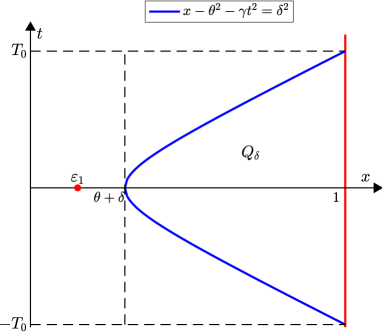
Figure 1: Set $Q_{\delta}$.

Henceforth $C,C_{0}>0$, etc. will denote generic constants which are independent of the parameter $s>0$, but can be dependent on other parameters such as $\lambda>0$. Since other parameters such as $\lambda$ are fixed, we do not specify the dependence of $C,C_{0}$, etc. on them.

We show the following result:

Lemma 4.10 (Hyperbolic Carleman estimate)

There exist constants $C>0$ and $s_{0}>0$ depending on $M$ and $r_{0}$, but independent of $s$ and the choices of $p$, such that

$$\int_{Q_{\delta}}(s|\partial_{x}y|^{2}+s|\partial_{t}y|^{2}+s^{3}|y|^{2})e^{2s\varphi}\,dxdt$$

$$\leq C\int_{Q_{\delta}}|F(x,t)|^{2}e^{2s\varphi}\,dxdt+C\int_{\partial Q_{\delta}}(s|\partial_{x}y|^{2}+s|\partial_{t}y|^{2}+s^{3}|y|^{2})e^{2s\varphi}dS$$

for all $s\geq s_{0}$ and $y\in H^{2}(Q_{\delta})$ satisfying

$$\partial_{t}^{2}y=\partial_{x}(p(x)\partial_{x}y)+F\quad\text{in }Q_{\delta}$$

with some $F\in L^{2}(Q_{\delta})$.

In particular, if $y(1,t)=\partial_{x}y(1,t)=0$ for $-T_{0}<t<T_{0}$, then

$$\int_{Q_{\delta}}(s|\partial_{x}y|^{2}+s|\partial_{t}y|^{2}+s^{3}|y|^{2})e^{2s\varphi}\,dxdt\leq C\int_{Q_{\delta}}|F(x,t)|^{2}e^{2s\varphi}\,dxdt+Cs^{3}e^{2se^{\lambda\delta^{2}}}\|y\|^{2}_{H^{2}(Q_{\delta})}$$ (48)

for all $s\geq s_{0}$ and $y\in H^{2}(Q_{\delta})$.

Proof of Lemma 4.10. This is a classical Carleman estimate: the proof can be done similarly to Theorem 4.2 in Bellassoued and Yamamoto [6] or Imanuvilov [19]. Here we omit the details of the proof. Estimate (48) can follow because $\psi(x,t)=\delta^{2}$ for $(x,t)\in\partial Q_{\delta}\setminus\{x=1\}$ and

$$\|\partial_{x}y\|_{L^{2}(\partial Q_{\delta})} +\|\partial_{t}y\|_{L^{2}(\partial Q_{\delta})}+\|y\|_{L^{2}(\partial Q_{\delta})}$$

$$\leq C(\|\partial_{x}y\|_{H^{1}(Q_{\delta})}+\|\partial_{t}y\|_{H^{1}(Q_{\delta})}+\|y\|_{H^{1}(Q_{\delta})})\leq C\|y\|_{H^{2}(Q_{\delta})}$$

by the trace theorem. $\square$

Remark 4.11

For Carleman estimates for hyperbolic equations, we usually have to assume a certain extra condition for the principal part $p(x)$ e.g., about the wave speed, and the extra condition is restrictive in higher spatial dimensions. However, the one spatial dimension case is exceptional and does not require any extra condition thanks to the smallness of the domain $Q_{\delta}$. More precisely, in the one dimensional case, such an extra condition is described as

$$\left|\frac{p^{\prime}(x)}{2p(x)}(x-\theta)\right|<1,\quad\theta+\delta\leq x\leq 1$$

(see e.g., Proposition 2.1 in Imanuvilov and Yamamoto [22]). Since $\displaystyle\max_{\theta+\delta\leq x\leq 1}|x-\theta|=1-\theta$ is sufficiently small, we see that

$$\left|\frac{p^{\prime}(x)}{2p(x)}(x-\theta)\right|\leq\frac{M}{2r_{0}}(1-\theta)<1.$$ (49)

Hence, there exists a constant $\mu_{*}(r_{0},M)>0$ such that if $0<1-\theta<\mu_{*}(r_{0},M)$, then (49) and so the Carleman estimate (48) hold.

In view of (49), the key Carleman (48) estimate holds near $x=1$ where Cauchy data are given, that is, for $\theta+\delta<x<1$. Thus, we first apply the Carleman estimate only for $\theta+\delta<x<1$ to prove that $f=0$ in $(\theta+\delta,\,1)$. This will be done in second step of the proof of Proposition 4.9. Next, we repeat the same argument by replacing $x=1$ by $x=\theta$, and this will be done in third step of the proof of Proposition 4.9.

Before proceeding to second step, we prove a Carleman estimate for a simple operator $\frac{d}{dx}$. We set

$$\varphi_{0}(x)=e^{\lambda(x-\theta)^{2}}$$

with fixed large constant $\lambda>0$.

Lemma 4.12

There exist constants $s_{0}>0$ and $C>0$ such that

$$s\int^{1}_{\theta+\delta}|f(x)|^{2}e^{2s\varphi_{0}(x)}\,dx\leq C\int_{\theta+\delta}^{1}|f^{\prime}|^{2}e^{2s\varphi_{0}}\,dx,$$

for all $s\geq s_{0}$ and all $f\in H^{1}(\theta+\delta,1)$ satisfying $f(1)=0$.

Proof of Lemma 4.12. The proof relies on the estimation of $h:=fe^{s\varphi_{0}}$ and the integration by parts, which is a conventional proof of the Carleman estimate.

We set

$$h(x):=f(x)e^{s\varphi_{0}(x)},\quad Lh(x):=e^{s\varphi_{0}(x)}\frac{d}{dx}(e^{-s\varphi_{0}(x)}h(x))=h^{\prime}(x)-s\varphi_{0}^{\prime}(x)h(x).$$

Then, integrating by parts and taking into account that $f(1)=0$, we have that there exists a positive constant $C$ such that

$$\int^{1}_{\theta+\delta}|f^{\prime}|^{2}e^{2s\varphi_{0}}\,dx =\int^{1}_{\theta+\delta}|Lh|^{2}dx=\int^{1}_{\theta+\delta}|h^{\prime}(x)-s\varphi_{0}^{\prime}(x)h(x)|^{2}\,dx$$

$$\geq-2s\int^{1}_{\theta+\delta}\varphi_{0}^{\prime}(x)h(x)h^{\prime}(x)\,dx=-s\int^{1}_{\theta+\delta}\varphi_{0}^{\prime}(x)\frac{d}{dx}h^{2}(x)\,dx$$

$$=\Big{[}s\varphi_{0}^{\prime}(x)h^{2}(x)\Big{]}^{x=\theta+\delta}_{x=1}+s\int^{1}_{\theta+\delta}\varphi_{0}^{\prime\prime}(x)h^{2}(x)\,dx$$

$$=2\lambda s\delta e^{\lambda\delta^{2}}h^{2}(\theta+\delta)+s\int^{1}_{\theta+\delta}(2\lambda\varphi_{0}(x)+4\lambda^{2}(x-\theta)^{2}\varphi_{0}(x))h^{2}(x)\,dx$$

$$\geq s\int^{1}_{\theta+\delta}2\lambda e^{\lambda(x-\theta)^{2}}h^{2}(x)\,dx\geq Cs\int^{1}_{\theta+\delta}|f|^{2}e^{2s\varphi_{0}}\,dx.$$

Thus, the proof of Lemma 4.12 is complete. $\square$

Second step of the proof of Proposition 4.9.

We take the even extension in $t$ of the solution $y$ of (45) to $(-\infty,0)$, and we denote it by the same letter:

$$y(x,t)=\left\{\begin{array}[]{ll}y(x,t),&\quad t\geq 0,\\ y(x,-t),&\quad t<0.\end{array}\right.$$

Also, for $R$, we make the even extension in $t<0$. Then, using that $y(\cdot,0)=\partial_{t}y(\cdot,0)=0$ and $\partial_{t}R(\cdot,0)=0$ on $[\varepsilon_{1},1]$ by (46), we can verify that

$$\left\{\begin{array}[]{l}\partial_{t}y,\,y\in H^{2}_{loc}((\varepsilon_{1},1)\times(-\infty,\infty)),\\[5.69054pt] \partial_{t}R,\,R\in L^{2}_{loc}(-\infty,\infty;H^{2}(\varepsilon_{1},1)),\\[5.69054pt] \partial_{t}\partial_{x}R,\,\partial_{t}\partial_{x}^{2}R\in L^{\infty}_{loc}((\varepsilon_{1},1)\times(-\infty,\infty))\end{array}\right.$$ (50)

and

$$\left\{\begin{array}[]{ll}\partial_{t}^{2}y=\partial_{x}(p(x)\partial_{x}y)+\partial_{x}(f(x)\partial_{x}R(x,t)),&\varepsilon_{1}<x<1,\,-\infty<t<\infty,\\[5.69054pt] y(1,t)=\partial_{x}y(1,t)=0,&-\infty<t<\infty,\\[5.69054pt] y(x,0)=\partial_{t}y(x,0)=0,&\varepsilon_{1}<x<1.\end{array}\right.$$ (51)

In (51), we see that $y,\partial_{t}y\in H^{2}((\varepsilon_{1},1)\times(-T,T))$ with arbitrarily given $T>0$. Setting

$$z:=\partial_{t}y\in H^{2}((\varepsilon_{1},1)\times(-T,T)),$$

and using (51), we have

$$\left\{\begin{array}[]{ll}\partial_{t}^{2}z=\partial_{x}(p(x)\partial_{x}z)+\partial_{x}(f(x)\partial_{t}\partial_{x}R(x,t)),&\varepsilon_{1}<x<1,\,-\infty<t<\infty,\\[5.69054pt] z(1,t)=\partial_{x}z(1,t)=0,&-\infty<t<\infty,\\[5.69054pt] z(x,0)=0,\quad\partial_{t}z(x,0)=\partial_{x}(f(x)\partial_{x}R(x,0)),&\varepsilon_{1}<x<1.\end{array}\right.$$ (52)

Notice that the second and the third conditions in (52) are obtained by (51) taking into account that $\partial_{t}^{2}y\in H^{1}(-T,T;L^{2}(\varepsilon_{1},1))$ and the Sobolev embedding such as $H^{1}(-T,T;L^{2}(\varepsilon_{1},1))\subset C^{0}([-T,T];L^{2}(\varepsilon_{1},1))$. Here, we also note that $\partial_{t}\partial_{x}^{2}y,\,\partial_{t}\partial_{x}^{2}R\in L^{2}(-T,T;L^{2}(\varepsilon_{1},1))$, and so $\partial_{x}^{2}y,\,\partial_{x}^{2}R\in C^{0}([-T,T];L^{2}(\varepsilon_{1},1))$ by the Sobolev embedding.

Setting now

$$M_{0}:=\|z\|_{H^{2}((\varepsilon_{1},1)\times(-T,T))}=\|\partial_{t}y\|_{H^{2}((\varepsilon_{1},1)\times(-T,T))},$$

by the regularity assumption (50) on $y$, we see that $M_{0}<\infty$.

Now, we apply the Carleman estimate (48) to (52) and we obtain that there exists a constant $C>0$, which is independent of $s>0$, such that

$$\int_{Q_{\delta}}(s|\partial_{x}z|^{2} +s|\partial_{t}z|^{2}+s^{3}|z|^{2})e^{2s\varphi}\,dxdt$$ (53)

$$\leq C\int_{Q_{\delta}}|\partial_{x}(f(x)\partial_{x}\partial_{t}R(x,t)|^{2}e^{2s\varphi}\,dxdt+Cs^{3}e^{2se^{\lambda\delta^{2}}}M_{0}^{2},$$

for all large $s>0$.

We set

$$w:=(\partial_{t}y)e^{s\varphi}=ze^{s\varphi}.$$

Then, direct calculations yield

$$\partial_{t}^{2}w=(\partial_{t}^{3}y)e^{s\varphi}+2s(\partial_{t}^{2}y)(\partial_{t}\varphi)e^{s\varphi}+(s\partial_{t}^{2}\varphi+s^{2}(\partial_{t}\varphi)^{2}))e^{s\varphi}\partial_{t}y.$$

On the other hand,

$$p\partial_{x}^{2}w=p(\partial_{x}^{2}\partial_{t}y)e^{s\varphi}+2ps(\partial_{t}\partial_{x}y)(\partial_{x}\varphi)e^{s\varphi}+p(s(\partial_{x}^{2}\varphi)+s^{2}(\partial_{x}\varphi)^{2}))e^{s\varphi}\partial_{t}y,$$

and also

$$p^{\prime}\partial_{x}w=p^{\prime}(\partial_{x}\partial_{t}y)e^{s\varphi}+sp^{\prime}(\partial_{x}\varphi)(\partial_{t}y)e^{s\varphi}.$$

Therefore, taking the derivative with respect to $t$ in (45) and multiplying by $e^{s\varphi}$, we can write

$$\partial_{t}^{2}w-\partial_{x}(p(x)\partial_{x}w)=e^{s\varphi}\partial_{x}(f(x)\partial_{x}\partial_{t}R(x,t))+P_{s}(w),$$ (54)

where the term $P_{s}(w)$ satisfies

$$\begin{array}[]{ll}|P_{s}(w)|&\leq Cs(|\partial_{t}^{2}y|+|\partial_{t}y|+|\partial_{x}\partial_{t}y|)e^{s\varphi}+Cs^{2}|\partial_{t}y|e^{s\varphi}\\[5.69054pt] &\leq C(s^{2}|w|+s|\partial_{t}w|+s|\partial_{x}w|),\qquad(x,t)\in Q_{\delta},\end{array}$$ (55)

for all large $s>0$. For the last inequality, we have used that $w=(\partial_{t}y)e^{s\varphi}$ and

$$(\partial_{t}^{2}y)e^{s\varphi}=\partial_{t}w-s(\partial_{t}\varphi)(\partial_{t}y)e^{s\varphi}=\partial_{t}w-s(\partial_{t}\varphi)w,$$

and

$$(\partial_{x}\partial_{t}y)e^{s\varphi}=\partial_{x}w-s(\partial_{x}\varphi)w,$$

which imply

$$|\partial_{t}^{2}y|e^{s\varphi}\leq|\partial_{t}w|+Cs|\partial_{t}y|e^{s\varphi}$$

and

$$|\partial_{x}\partial_{t}y|e^{s\varphi}\leq|\partial_{x}w|+Cs|\partial_{t}y|e^{s\varphi},$$

respectively.

On the other hand, we it is not difficult to see that we can write (53) in terms of $w=ze^{s\varphi}=(\partial_{t}y)e^{s\varphi}$

$$\begin{array}[]{l}\displaystyle\int_{Q_{\delta}}(s|\partial_{x}w|^{2}+s|\partial_{t}w|^{2}+s^{3}|w|^{2})\,dxdt\\[11.38109pt] \phantom{------}\leq\displaystyle C\int_{Q_{\delta}}(\partial_{x}(f(x)\partial_{x}\partial_{t}R(x,t))|^{2}e^{2s\varphi}\,dxdt+Cs^{3}e^{2se^{\lambda\delta^{2}}}M_{0}^{2},\end{array}$$ (56)

for all large $s>0$.

Multiplying (54) by $2\partial_{t}w$ and integrating over $Q_{\delta}^{-}:=Q_{\delta}\cap\{t<0\}$ (see Figure 2), we have

$$B: =2\int_{Q_{\delta}^{-}}(\partial_{t}^{2}w)\partial_{t}w\,dxdt-2\int_{Q_{\delta}^{-}}\partial_{x}(p(x)\partial_{x}w)\partial_{t}w\,dxdt$$ (57)

$$=2\int_{Q_{\delta}^{-}}(f^{\prime}(x)\partial_{t}\partial_{x}R+f\partial_{t}\partial_{x}^{2}R)e^{s\varphi}\partial_{t}w\,dxdt+2\int_{Q_{\delta}^{-}}P_{s}(w)\partial_{t}w\,dxdt.$$

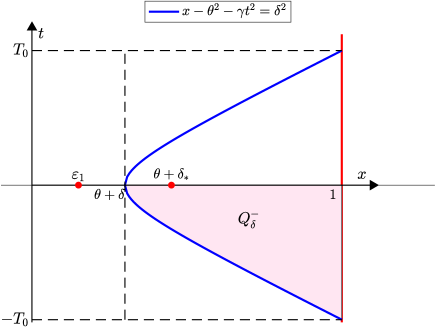
Figure 2: Set $Q_{\delta}^{-}$.

Then, integration by parts in the left hand side of (57) yields

$$B=\int_{Q_{\delta}^{-}}\partial_{t}(|\partial_{t}w|^{2})\,dxdt+2\int_{Q_{\delta}^{-}}p(x)(\partial_{x}w)(\partial_{t}\partial_{x}w)\,dxdt-2\int_{\partial Q_{\delta}^{-}}p(x)(\partial_{x}w)(\partial_{t}w)\nu_{x}\,dS.$$

Here and henceforth let $\nu=(\nu_{x},\nu_{t})$ be the unit outward normal vector to $\partial Q_{\delta}^{-}$ in the $(x,t)$-space. We have $\nu_{x}=0$ and $\nu_{t}=1$ on $t=0$. Since $w=(\partial_{t}y)e^{s\varphi}$ and $y(1,0)=0$, we have that $\partial_{t}w(1,t)=\partial_{t}((\partial_{t}y)e^{s\varphi})(1,t)=0$. Moreover, using that

$$\partial Q_{\delta}^{-}=(\partial Q_{\delta}^{-}\cap\{x=1\})\cup(\partial Q_{\delta}^{-}\cap\{x<1\})=(\partial Q_{\delta}^{-}\cap\{x=1\})\cup(\partial Q_{\delta}^{-}\cap\{\psi(x,t)=\delta^{2}\}),$$

we obtain

$$\left|-2\int_{\partial Q_{\delta}^{-}}p(\partial_{x}w)(\partial_{t}w)\nu_{x}\,dS\right|=\left|-2\int_{\partial Q_{\delta}^{-}\cap\{\psi(x,t)=\delta^{2}\}}p(\partial_{x}w)(\partial_{t}w)\nu_{x}dS\right|$$

$$\leq \left|-2\int_{\partial Q_{\delta}^{-}\cap\{\psi(x,t)=\delta^{2}\}}p(\partial_{x}\partial_{t}y+s(\partial_{x}\varphi)\partial_{t}y)(\partial_{t}^{2}y+s(\partial_{t}\varphi)\partial_{t}y)e^{2se^{\lambda\delta^{2}}}\nu_{x}dS\right|$$

$$\leq Ce^{2se^{\lambda\delta^{2}}}s^{2}\int_{\partial Q_{\delta}^{-}}(|\partial_{x}\partial_{t}y|^{2}+|\partial_{t}^{2}y|^{2}+|\partial_{t}y|^{2})\,dS$$

$$\leq Cs^{2}e^{2se^{\lambda\delta^{2}}}(\|\partial_{x}\partial_{t}y\|_{H^{1}(Q_{\delta})}^{2}+\|\partial_{t}^{2}y\|_{H^{1}(Q_{\delta})}^{2}+\|\partial_{t}y\|_{H^{1}(Q_{\delta})}^{2})\leq Cs^{2}e^{2se^{\lambda\delta^{2}}}M_{0}^{2},$$

for all large $s>0$. Hence,

$$\left|-2\int_{\partial Q_{\delta}^{-}}p(\partial_{x}w)(\partial_{t}w)\nu_{x}\,dS\right|\leq Cs^{2}e^{2se^{\lambda\delta^{2}}}M_{0}^{2}.$$ (58)

In the last inequality, we have used the trace theorem in $Q_{\delta}^{-}$.

Moreover, using that $\partial_{t}y(x,0)=0$ for $\theta+\delta<x<1$, we have

$$\partial_{x}w(x,0)=\partial_{x}(e^{s\varphi}\partial_{t}y)|_{t=0}=0,\quad\theta+\delta<x<1.$$

Hence, integration by parts yields

$$2\int_{Q_{\delta}^{-}}p(x)(\partial_{x}w)\partial_{t}\partial_{x}w\,dxdt =\int_{Q_{\delta}^{-}}p(x)\partial_{t}(|\partial_{x}w|^{2})\,dxdt$$

$$=\int^{1}_{\theta+\delta}p(x)|\partial_{x}w(x,0)|^{2}\,dx+\int_{\partial Q_{\delta}^{-}}p(x)|\partial_{x}w|^{2}\nu_{t}\,dS.$$

Since $\partial_{t}y(x,0)=0$ for $\varepsilon_{1}<x<1$ implies $\partial_{x}w(x,0)=0$ for $\theta+\delta<x<1$, similarly to (58), by integration by parts, we can estimate the above integral on $\partial Q_{\delta}^{-}$ to see

$$\left|2\int_{Q_{\delta}^{-}}p(\partial_{x}w)\partial_{t}\partial_{x}w\,dxdt\right|=\left|\int_{\partial Q_{\delta}^{-}}p|\partial_{x}w|^{2}\nu_{t}\,dS\right|\leq Cs^{2}e^{2se^{\lambda\delta^{2}}}M_{0}^{2}.$$

Furthermore, we have

$$\int_{Q_{\delta}^{-}}\partial_{t}(|\partial_{t}w|^{2})\,dxdt=\int^{1}_{\theta+\delta}|\partial_{t}w(x,0)|^{2}\,dx+\int_{\partial Q_{\delta}^{-}}|\partial_{t}w|^{2}\nu_{t}\,dS$$

$$\geq \int^{1}_{\theta+\delta}|\partial_{t}w(x,0)|^{2}\,dx-Cs^{2}e^{2se^{\lambda\delta^{2}}}M_{0}^{2}.$$

Therefore,

$$|B|\geq\int^{1}_{\theta+\delta}|\partial_{t}w(x,0)|^{2}dx-Cs^{2}e^{2se^{\lambda\delta^{2}}}M_{0}^{2}.$$ (59)

On the other hand, by (46) and (55), we can estimate the right-hand side of (57) as follows:

$$\left|2\int_{Q_{\delta}^{-}}(f^{\prime}(x)\partial_{t}\partial_{x}R+f(x)\partial_{t}\partial_{x}^{2}R)e^{s\varphi}\partial_{t}wdxdt+2\int_{Q_{\delta}^{-}}P_{s}(w)\partial_{t}wdxdt\right|$$

$$\leq C\int_{Q_{\delta}^{-}}(|f^{\prime}(x)|+|f(x)|)e^{s\varphi}|\partial_{t}w|\,dxdt+C\int_{Q_{\delta}^{-}}(s^{2}|w|+s|\partial_{x}w|+s|\partial_{t}w|)|\partial_{t}w|\,dxdt.$$

Applying the Cauchy-Schwarz inequality to the right-hand side and using

$$s^{2}|w||\partial_{t}w|=s^{\frac{3}{2}}|w|s^{\frac{1}{2}}|\partial_{t}w|\leq s^{3}|w|^{2}+s|\partial_{t}w|^{2},$$

by (56) and (46) we can obtain

$$\Big{|}\text{[the right-hand side of (\ref{eq57})]}\Big{|}$$

$$\leq C\int_{Q_{\delta}}(|f^{\prime}(x)|+|f(x)|)e^{2s\varphi}\,dxdt+C\int_{Q_{\delta}}|\partial_{x}(f\partial_{x}\partial_{t}R)|^{2}e^{2s\varphi}\,dxdt+Cs^{3}e^{2se^{\lambda\delta^{2}}}M_{0}^{2}$$

$$\leq C\int_{Q_{\delta}}(|f^{\prime}(x)|+|f(x)|)e^{2s\varphi}\,dxdt+Cs^{3}e^{2se^{\lambda\delta^{2}}}M_{0}^{2}.$$

Therefore, in view of (59), we reach

$$\int_{\theta+\delta}^{1}|\partial_{t}w(x,0)|^{2}\,dx\leq C\int_{Q_{\delta}}(|f^{\prime}(x)|^{2}+|f(x)|^{2})e^{2s\varphi(x,t)}dxdt+Cs^{3}e^{2se^{\lambda\delta^{2}}}M_{0}^{2},$$ (60)

for all large $s>0$.

Now, we recall that $T_{0}=\sqrt{\frac{(1-\theta)^{2}-\delta^{2}}{\gamma}}$ and that $w=(\partial_{t}y)e^{s\varphi}$. By (45) we have

$$\partial_{t}w(x,0) =\partial_{t}^{2}y(x,0)e^{s\varphi(x,0)}+(\partial_{t}y)(x,0)(\partial_{t}e^{s\varphi})(x,0)$$

$$=\partial_{t}^{2}y(x,0)e^{s\varphi(x,0)}=\partial_{x}(f(x)\partial_{x}R(x,0))e^{s\varphi(x,0)}.$$

Hence, (60) yields

$$\begin{array}[]{l}\displaystyle\int^{1}_{\theta+\delta}|f^{\prime}(x)\partial_{x}R(x,0)+f(x)\partial_{x}^{2}R(x,0)|^{2}e^{2s\varphi(x,0)}\,dx\\[11.38109pt] \leq C\displaystyle\int_{Q_{\delta}}(|f(x)|^{2}+|f^{\prime}(x)|^{2})e^{2s\varphi(x,t)}\,dxdt+Cs^{3}e^{2se^{\lambda\delta^{2}}}M_{0}^{2},\end{array}$$ (61)

for all large $s>0$.

Since

$$\varphi(x,t)-\varphi(x,0)=-e^{\lambda|x-\theta|^{2}}(1-e^{-\lambda\gamma t^{2}})\leq-(1-e^{-\lambda\gamma t^{2}}),$$

by (47) we obtain

$$\int_{Q_{\delta}}(|f(x)|^{2}+|f^{\prime}(x)|^{2})e^{2s\varphi(x,t)}\,dxdt\leq C\int^{T_{0}}_{-T_{0}}\left(\int^{1}_{\theta+\delta}(|f|^{2}+|f^{\prime}|^{2})e^{2s\varphi(x,0)}\,dx\right)e^{2s(\varphi(x,t)-\varphi(x,0))}\,dt$$

$$\leq C\int^{1}_{\theta+\delta}\left(\int^{T_{0}}_{-T_{0}}e^{-2s(1-e^{-\lambda\gamma t^{2}})}dt\right)(|f|^{2}+|f^{\prime}|^{2})e^{2s\varphi(x,0)}\,dx.$$

The Lebesgue convergence theorem yields

$$\int^{T_{0}}_{-T_{0}}e^{-2s(1-e^{-\lambda\gamma t^{2}})}dt=o(1)$$

as $s\to\infty$, and so

$$\int_{Q_{\delta}}|f(x)|^{2}+|f^{\prime}(x)|^{2})e^{2s\varphi(x,t)}\,dxdt=o(1)\int^{1}_{\theta+\delta}(|f(x)|^{2}+|f^{\prime}(x)|^{2})e^{2s\varphi(x,0)}\,dx.$$

Applying this in (61), we reach

$$\int^{1}_{\theta+\delta}|f^{\prime}(x)\partial_{x}R(x,0)+f(x)\partial_{x}^{2}R(x,0)|^{2}e^{2s\varphi(x,0)}\,dx$$

$$\leq o(1)\int^{1}_{\theta+\delta}(|f(x)|^{2}+|f^{\prime}(x)|^{2})e^{2s\varphi(x,0)}\,dx+Cs^{3}e^{2se^{\lambda\delta^{2}}}M_{0}^{2}$$ (62)

for all large $s>0$.

Using now that $|\partial_{x}R(x,0)|\geq r_{0}>0$ for all $x\in[\varepsilon_{1},1]$ and $\partial_{x}^{2}R(\cdot,0)\in L^{\infty}(\varepsilon_{1},1)$ by (46), we see

$$\int^{1}_{\theta+\delta}|f^{\prime}(x)\partial_{x}R(x,0)+f(x)\partial_{x}^{2}R(x,0)|^{2}e^{2s\varphi(x,0)}\,dx$$

$$\geq r_{0}^{2}\int^{1}_{\theta+\delta}|f^{\prime}(x)|^{2}e^{2s\varphi(x,0)}\,dx-C\int^{1}_{\theta+\delta}|f(x)|^{2}e^{2s\varphi(x,0)}\,dx.$$

Hence, (4.2.2) yields

$$r_{0}^{2}\int^{1}_{\theta+\delta}|f^{\prime}(x)|^{2}e^{2s\varphi(x,0)}dx-C\int^{1}_{\theta+\delta}|f(x)|^{2}e^{2s\varphi(x,0)}dx$$

$$\leq o(1)\int^{1}_{\theta+\delta}|f^{\prime}(x)|^{2}e^{2s\varphi(x,0)}dx+o(1)\int^{1}_{\theta+\delta}|f(x)|^{2}e^{2s\varphi(x,0)}dx+Cs^{3}e^{2se^{\lambda\delta^{2}}}M_{0}^{2},$$

for all large $s>0$. Absorbing the first term on the right-hand side into the left-hand side. we reach

$$\int^{1}_{\theta+\delta}|f^{\prime}(x)|^{2}e^{2s\varphi(x,0)}dx\leq C\int^{1}_{\theta+\delta}|f(x)|^{2}e^{2s\varphi(x,0)}dx\\ +Cs^{3}e^{2se^{\lambda\delta^{2}}}M_{0}^{2},$$

for all large $s>0$. Applying Lemma 4.12 to the first term on the right-hand side if this inequality, we obtain

$$C_{2}\int^{1}_{\theta+\delta}|f^{\prime}(x)|^{2}e^{2s\varphi(x,0)}dx-\frac{C}{s}\int^{1}_{\theta+\delta}|f^{\prime}(x)|^{2}e^{2s\varphi(x,0)}dx\leq Cs^{3}e^{2se^{\lambda\delta^{2}}}M_{0}^{2},$$

for all large $s>0$. Choosing $s>0$ sufficiently large, we can absorb the second term into the first term on the left-hand side, and we reach

$$C_{3}\int^{1}_{\theta+\delta}|f^{\prime}(x)|^{2}e^{2s\varphi(x,0)}dx\leq Cs^{3}e^{2se^{\lambda\delta^{2}}}M_{0}^{2},$$ (63)

for all large $s>0$.

Next, choose $\delta_{*}>\delta$ such that $\theta+\delta_{*}<1$ (see Figure 2). Then

$$\varphi(x,0)=e^{\lambda(x-\theta)^{2}}\geq e^{\lambda\delta_{*}^{2}}>e^{\lambda\delta^{2}}\quad\mbox{for $\theta+\delta_{*}\leq x\leq 1$},$$

and so (63) yields

$$C_{3}e^{2se^{\lambda\delta_{*}^{2}}}\|f^{\prime}\|^{2}_{L^{2}(\theta+\delta_{*},1)}\leq C_{3}\int^{1}_{\theta+\delta_{*}}|f^{\prime}(x)|^{2}e^{2s\varphi(x,0)}dx$$

$$\leq C_{3}\int^{1}_{\theta+\delta}|f^{\prime}(x)|^{2}e^{2s\varphi(x,0)}dx\leq Cs^{3}e^{2se^{\lambda\delta^{2}}}M_{0}^{2},$$

that is,

$$\|f^{\prime}\|^{2}_{L^{2}(\theta+\delta_{*},1)}\leq C_{4}s^{3}M_{0}^{2}\exp(-2s(e^{\lambda\delta_{*}^{2}}-e^{\lambda\delta^{2}})),$$

for all large $s>0$. By $e^{\lambda\delta_{*}^{2}}-e^{\lambda\delta^{2}}>0$, letting $s\to\infty$, we see that $f^{\prime}=0$ in $(\theta+\delta_{*},\,1)$. Since $\theta_{*}>\theta$ is arbitrary, we deduce that $f^{\prime}=0$ in $(\theta+\delta,\,1)$. Since $f(1)=0$, we see that $f=0$ in $(\theta+\delta,\,1)$.

Third step of the proof of Proposition 4.9: continuation of the uniqueness of $f$ and $y$ toward $x=\varepsilon_{1}$.

Substituting $f=0$ in $(\theta+\delta,1)$ in (51), we have

$$\left\{\begin{array}[]{rl}&\partial_{t}^{2}y=\partial_{x}(p(x)\partial_{x}y),\quad\theta+\delta<x<1,\,-\infty<t<\infty,\\ &y(1,t)=\partial_{x}y(1,t)=0,\quad-\infty<t<\infty.\end{array}\right.$$ (64)

We apply (48) to (64) and obtain

$$\int_{Q_{\delta}}s^{3}|y|^{2}e^{2s\varphi}\,dxdt\leq Cs^{3}e^{2se^{\lambda\delta^{2}}}M_{0}^{2}$$

for all large $s>0$. Hence, choosing $\delta_{*}>\delta$ again such that $\theta+\delta_{*}<1$, and using that $Q_{\delta}\supset Q_{\delta_{*}}$, we have

$$s^{3}e^{2se^{\lambda\delta_{*}^{2}}}\|y\|^{2}_{L^{2}(Q_{\delta_{*}})}\leq\int_{Q_{\delta_{*}}}s^{3}|y|^{2}e^{2s\varphi}\,dxdt\leq\int_{Q_{\delta}}s^{3}|y|^{2}e^{2s\varphi}\,dxdt\leq Cs^{3}e^{2se^{\lambda\delta^{2}}}M_{0}^{2},$$

that is,

$$\|y\|^{2}_{L^{2}(Q_{\delta_{*}})}\leq C\exp(-2s(e^{\lambda\delta_{*}^{2}}-e^{\lambda\delta^{2}}))M_{0}^{2},$$

for all large $s>0$. Letting $s\to\infty$, we obtain $y=0$ in $Q_{\delta_{*}}$. Since $\delta_{*}>\delta$ is arbitrary, we have $y=0$ in $Q_{\delta}$ as well as $f=0$ in $(\theta+\delta,1)$. Since also $\delta>0$ is arbitrary, we see that

$$\left\{\begin{array}[]{rl}&y=0\quad\mbox{in $Q_{0}:=\{(x,t);\,-\infty<t<\infty,\quad\theta<x<1,\quad\psi(x,t)>0\}$ },\\ &f=0\quad\mbox{in $(\theta,1)$}.\end{array}\right.$$

We note that

$$Q_{0}=\left\{(x,t);\,|t|<\frac{1}{\sqrt{\gamma}}(x-\theta),\,\,\theta<x<1\right\}.$$

For arbitrary $t_{0}\in\mathds{R}$, we repeat the same arguments to (64) with translated time variable $t-t_{0}$, so that

$$y=0\quad\mbox{in $\left\{(x,t);\,|t-t_{0}|<\frac{1}{\sqrt{\gamma}}(x-\theta),\,\,\theta<x<1\right\}$}.$$

Since $t_{0}\in\mathds{R}$ is arbitrary, we see that

$$y=0\quad\mbox{in $\bigcup_{t_{0}\in\mathds{R}}\left\{(x,t);\,|t-t_{0}|<\frac{1}{\sqrt{\gamma}}(x-\theta),\,\,\theta<x<1\right\}\supset(\theta,1)\times(-\infty,\infty)$}.$$

Using this with (45), we derive

$$\left\{\begin{array}[]{l}\partial_{t}^{2}y=\partial_{x}(p(x)\partial_{x}y)+\partial_{x}(f(x)\partial_{x}R(x,t)),\quad\varepsilon_{1}<x<\theta,\,-\infty<t<\infty,\\[2.84526pt] y(\theta,t)=\partial_{x}y(\theta,t)=0,\quad-\infty<t<\infty,\\[2.84526pt] y(x,0)=\partial_{t}y(x,0)=0,\quad\varepsilon_{1}<x<\theta.\end{array}\right.$$

Now, starting at $x=1$, we advance by the width $\theta$ to obtain the uniqueness from $x=1$ to $x=\theta$. In the second step of this proof, we have applied the Carleman estimate in $Q_{\delta}\subset\{x;\,1-(1-\theta)<x<1\}$ with the weight function $\psi(x,t)=(x-\theta)^{2}-\gamma t^{2}$. Now we have to consider a level set in $\{x;\,\theta-(1-\theta))<x<\theta\}$ and so we shift the level set $Q_{\delta}$ by $x\mapsto x-(\theta-1)$:

$$Q^{1}_{\delta}:=\{(x,t);\,-\infty<t<\infty,\quad\psi^{1}(x,t)>\delta^{2}\},$$

where

$$\psi^{1}(x,t):=((x-(\theta-1))-\theta)^{2}-\gamma t^{2}.$$

Since $1-\theta>0$ is sufficiently small, by Remark 4.11 we can verify the Carleman estimate from Lemma 4.10 in $Q^{1}_{\delta}$. Then we repeat the same argument fro the second step of this proof by replacing the $x$-interval $(\varepsilon_{1},1)$ by $(\varepsilon_{1},\theta)$ and we can prove

$$y(x,t)=0,\quad(x,t)\in(1-2(1-\theta),\,1-(1-\theta))\times(-\infty,\infty)$$

and

$$f(x)=0,\quad x\in(1-2(1-\theta),\,1-(1-\theta)).$$

Adjusting the weight function for the Carleman estimate and continuing this argument, we reach

$$f(x)=0,\quad x\in(1-k(1-\theta),\,1),$$

with $k\in\mathds{N}$ as long as $1-k(1-\theta)>\varepsilon_{1}$.

We choose $k_{0}\in\mathds{N}$ such that

$$1-(k_{0}+1)(1-\theta)<\varepsilon_{1}<1-k_{0}(1-\theta).$$

Then, $(1-k_{0}(1-\theta))-\varepsilon_{1}<1-\theta$ and

$$f=0\quad\mbox{in $(1-k_{0}(1-\theta),\,1)$}.$$ (65)

Since we have $1-\theta>0$ can be arbitrarily small, we can choose $\theta>0$ and $k_{0}\in\mathds{N}$ such that $1-k_{0}(1-\theta)>\varepsilon_{1}$ and $1-k_{0}(1-\theta)$ is arbitrarily close to $\varepsilon_{1}$. By the continuity of $f$, we reach $f=0$ in $(\varepsilon_{1},1)$.

Thus, the proof of Proposition 4.9 is complete. $\square$

4.2.3 Third Step: Completion of the proof of Theorem 4.2

Now we proceed to finish the proof of Theorem 4.2. Recall that we have assumed (28). Then, Lemma 4.8 yields

$$\partial_{x}\widetilde{u}_{a,\alpha}(1,t)=\partial_{x}\widetilde{u}_{b,\beta}(1,t),\quad 0<t<\infty.$$

Here $\widetilde{u}_{a,\alpha}$ and $\widetilde{u}_{b,\beta}$ are the solutions to (32) corresponding to $(a,\alpha)$ and $(b,\beta)$, respectively. Setting

$$p(x)=x^{\alpha}a(x)\quad y=\widetilde{u}_{a,\alpha}-\widetilde{u}_{b,\beta},\quad f=x^{\alpha}a(x)-x^{\beta}b(x),\quad R(x,t)=\widetilde{u}_{b,\beta}(x,t),$$

we have (45) and $\partial_{x}y(1,t)=0$ for $t>0$.

In view of Proposition 4.9, using the regularity (33)-(35) of $y$ and $R$ guaranteed by Lemma 4.5, we obtain $f=0$ in $\varepsilon_{1}<x<1$. Thus, the proof of Theorem 4.2 is complete. $\square$

5 Numerical results

In this section, we will consider numerical results for the previous inverse problems. We will carry out the reconstruction of the unknown functions $a$ and the power $\alpha$ through the resolution of some appropriate extremal problems. This strategy has been applied in some previous papers for other similar problems, see [2] and [13]. The results of the numerical tests that follow pretend to illustrate the theoretical results in the previous sections.

5.1 Numerical tests for the linear case I

In this section we present the numerical reconstruction of the constant coefficient $a$ in (10) by distributed measurements, related to the theoretical result from Theorem 3.1. More precisely, we will deal with the following inverse problem: given $t_{0}\in(0,T)$ as in (12), $u_{0}=u_{0}(x)$, $\gamma=\partial_{t}u(\cdot,t_{0})$ and $\beta=u(\cdot,t_{0})$, find $a\in\mathcal{U}^{a}_{ad}$ such that the corresponding solution $u^{a}$ of (10) satisfies the additional conditions:

$$\partial_{t}u^{a}(x,t_{0})=\gamma(x),\quad x\partial_{x}u^{a}(x,t_{0})=\beta(x),\quad\forall\,x\in(0,\ell),$$

where the admissible set $\mathcal{U}^{a}_{ad}=\{a:0<\underline{a}\leq a\leq\overline{a}\}$.

We reformulate the inverse problem as the following extremal problem: find $a\in\mathcal{U}^{a}_{ad}$ such that

$$J(a)\leq J(a^{\prime}),\quad\forall\,a^{\prime}\in\mathcal{U}^{a}_{ad}\,,$$ (66)

where the functional $J:a\in\mathcal{U}^{a}_{ad}\mapsto\mathds{R}$ is given by

$$J(a)=\dfrac{1}{2}\displaystyle\int_{0}^{\ell}|\gamma(x)-\partial_{t}u^{a}(x,t_{0})|^{2}\,dx+\dfrac{1}{2}\displaystyle\int_{0}^{\ell}|\beta(x)-x\partial_{x}u^{a}(x,t_{0})|^{2}\,dx,$$ (67)

with $u^{a}$ the solution of (10) corresponding to the unknown $a$.

We have performed several numerical tests with different values of $a$ to recover: $a>1$, $a=1$ and $a<1$. In them, we fix $T=5$, $\ell=1$ and $u_{0}(x)=0.5x^{2}(1-x)$. In the first three tests we will take, for simplicity, $f(x,t)=0$. We will denote by $a_{d}$ the desired value of $a$ that we would like to obtain and by $a_{i}$ the initial guess for the optimization algorithm. Using an optimization algorithm from Optimization Toolbox of MatLab, the fmincon function and interior-point gradient based algorithm, we have computed $a_{c}$. Our goal is to obtain $a_{c}$ as close as possible to $a_{d}$.

Test 1

Let us take $a_{i}=0.7$ as an initial guess for the minimization algorithm and $t_{0}=0.2$, that we have computed numerically such that (12) holds. The desired value to recover is $a_{d}=1.7$. After numerical resolution of the optimization problem (66), we found $a_{c}=1.7$. The numerical results can be seen in Figure 4, where the desired $a_{d}$ and computed $a_{c}$ have been represented. In Figure 4 we have plotted the evolution of the cost at each iteratios of the optimization algorithm represented by blue points. In Table 5.1 we can see the evolution of the cost when we introduce random noises in the target.

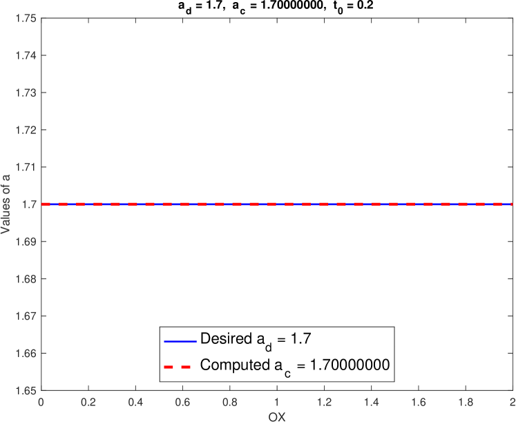
Figure 3: Test 1, $a_{d}$ solid line, $a_{c}$ dashed line.

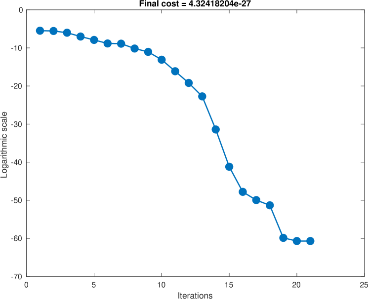
Figure 4: Test 1, the evolution of the cost.

Table 1: Cost at the best stopping and computed $a_{c}$ with random noises in the target in Test 1.

% noise	Cost	Iterations	$a_{c}$
1%	1.e-7	17	1.70451153
0.1%	1.e-8	16	1.70017891
0.01%	1.e-10	16	1.70017665
0.001%	1.e-13	15	1.70000362
0%	1.e-27	20	1.7

Figure 5: Test 1, numerical illustration of stability.

Remark 5.1 (Numerical illustration of stability)

In order to illustrate the stability of the considered inverse problem in the Test  1, we have represented in Figure 5 as points the quotients

$$K_{j}=\dfrac{|a-a^{\ast}|}{\|\gamma(x)-\gamma_{j}^{\ast}(x)\|+\|\beta(x)-\beta_{j}^{\ast}(x)\|},\quad j=1\dots,50,$$ (68)

where $\gamma(x)=\partial_{t}u^{a}(x,t_{0})$, $\beta(x)=x\partial_{x}u^{a}(x,t_{0})$ and for all $j$, $\gamma^{\ast}_{j}(x)=\gamma(x)+\varepsilon_{j}$, $\beta^{\ast}_{j}(x)=\beta(x)+\varepsilon_{j}$ with the $\varepsilon_{j}$ random perturbations in $(0,0.05)$. We can see that all the quotients $K_{j}$ are bounded.

Test 2

Let us now take $a_{i}=0.2$, $t_{0}=0.2$ and the desired value to recover $a_{d}=1$. The optimization algorithm gives $a_{c}=1$, see Figure 6. In Table 5.1 we can see the evolution of the cost when we introduce random noises in the target.

Table 2: Evolution of the cost and computed $a_{c}$ with random noises in the target in Test 2.

% noise	Cost	Iterations	$a_{c}$
1%	1.e-6	12	0.99670260
0.1%	1.e-8	13	1.00012771
0.01%	1.e-14	10	0.99995171
0.001%	1.e-13	14	0.99999488
0%	1.e-24	14	1

Figure 6: Test 2, the evolution of the cost.

Test 3

Let us take $a_{i}=0.7$ as an initial guess for the minimization algorithm, $t_{0}=0.2$ and $a_{d}=0.2$. The numerical resolution of the optimization problem gives $a_{c}=0.2$ (see Figure 7 and Table 5.1).

Table 3: Evolution of the cost and computed $a_{c}$ with random noises in the target in Test 3.

% noise	Cost	Iterations	$a_{c}$
1%	1.e-7	11	0.20046140
0.1%	1.e-13	9	0.19997676
0.01%	1.e-11	16	0.19999893
0.001%	1.e-13	14	0.20000028
0%	1.e-27	16	0.2

Figure 7: Test 3, the evolution of the cost.

Test 4

We consider a non-homogeneous problem (10) with $f(x,t)=2xt$. Let us take $a_{i}=0.7$ and $t_{0}=0.4$. The desired value is $a_{d}=1.7$. The numerical resolution of the optimization problem gives $a_{c}=1.7$. Figure 9 shows the evolution of iterations of the optimization algorithm and Figure 9 the evolution of the cost. In Table 5.1 we present the results with random noises in the target and Figure 10 representes the solution corresponding to the computed $a_{c}$.

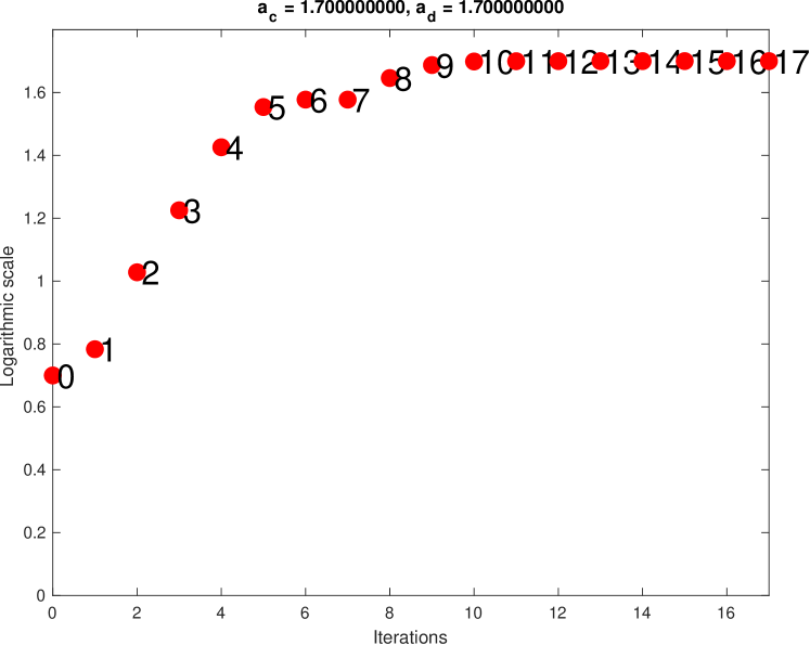
Figure 8: Test 4, iterations of the algorithm.

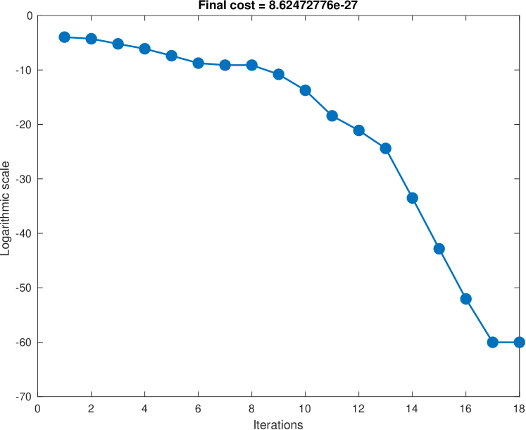
Figure 9: Test 4, the evolution of the cost.

Table 4: Cost at the best stopping and $a_{c}$ with random noises in the target in Test 4.

% noise	Cost	Iterations	$a_{c}$
1%	1.e-7	14	1.69767371
0.1%	1.e-8	15	1.69992839
0.01%	1.e-11	18	1.69997876
0.001%	1.e-12	15	1.69999972
0%	1.e-27	17	1.7

Figure 10: Test 4, computed solution $u=u(x,t)$.

5.2 Numerical tests for the linear case II

In this section we will present some numerical results for second inverse problem of identification of $a$ from one boundary observation $u_{x}(1,t)$, mentioned at the beginning of the Section 3.1. Arguing as in the previous section, we reformulate the inverse problem as an optimization problem (66), where the funcional $J:a\in\mathcal{U}^{a}_{ad}\mapsto\mathds{R}$ is now given by

$$J(a)=\dfrac{1}{2}\displaystyle\int_{0}^{T}|\eta(t)-\partial_{x}u^{a}(1,t)|^{2}\,dt,$$ (69)

where $\eta=\partial_{x}u(1,\cdot)$ is given and $u^{a}$ is the solution of (10) corresponding to the unknown $a$.

In what follows we present some numerical tests for this inverse problem. We will consider the same data as in the previous section: $T=5$, $\ell=1$, $u_{0}(x)=0.5x^{2}(1-x)$ and $f(x,t)=0$. In order to simplify the presentation, we will show just the evolution of the cost and the results with random noises.

Test 5

We take $a_{i}=0.7$ as an initial guess for the minimization algorithm. The desired value is $a_{d}=1.7$. The results of the numerical computations are presented in Table 5.2 and Figure 11.

Table 5: Evolution of the cost and computed $a_{c}$ with random noises in the target in Test 5.

% noise	Cost	Iterations	$a_{c}$
1%	1.e-6	13	1.69198034
0.1%	1.e-8	13	1.70001564
0.01%	1.e-14	10	1.70009682
0.001%	1.e-18	12	1.70000143
0%	1.e-25	18	1.7

Figure 11: Test 5, the evolution of the cost.

Test 6

Taking $a_{i}=0.2$ and $a_{d}=1$, we can see the numerical results in Figure 12 and Table 5.2.

Table 6: Evolution of the cost and computed $a_{c}$ with random noises in the target in Test 6.

% noise	Cost	Iterates	$a_{c}$
1%	1.e-6	10	0.99701925
0.1%	1.e-8	13	1.00058988
0.01%	1.e-9	16	0.99994514
0.001%	1.e-13	12	0.99999587
0%	1.e-27	13	1

Figure 12: Test 6, the evolution of the cost.

Test 7

Taking $a_{i}=0.7$ and $a_{d}=0.2$, Figure 13 and Table 5.2 show the numerical results.

Table 7: Evolution of the cost and computed $a_{c}$ with random noises in the target in Test 7.

% noise	Cost	Iterations	$a_{c}$
1%	1.e-5	15	0.20127090
0.1%	1.e-8	15	0.20020541
0.01%	1.e-9	14	0.19997384
0.001%	1.e-11	14	0.20000100
0%	1.e-28	18	0.2

Figure 13: Test 7, the evolution of the cost.

5.3 Numerical tests for the power-like case I

We will present in this section some numerical results of the reconstruction of $\alpha$ for weak and strong degenerate cases (16) and (17) from data that appear in Theorem 3.7. More precisely, given $t_{0}\in(0,T)$ as in (20), $u_{0}=u_{0}(x)$ and $\ell<1$, in order to reconstruct $\alpha$ we will solve numerically the following optimization problem: find $\alpha\in(0,2)$ such that

$$J(\alpha)\leq J(\alpha^{\prime}),\quad\forall\,\alpha^{\prime}\in(0,2),$$ (70)

where the functional $J:(0,2)\mapsto\mathds{R}$ is given by

$$J(\alpha)=\dfrac{1}{2}\displaystyle\int_{0}^{1}|\gamma(x)-\partial_{t}u^{\alpha}(x,t_{0})|^{2}\,dx+\dfrac{1}{2}\displaystyle\int_{0}^{1}|\beta(x)-x^{2}\partial_{x}u^{\alpha}(x,t_{0})|^{2}\,dx,$$

with $u^{\alpha}$ the corresponding solution of (16) or (17) assoceated to the unknown power $\alpha$.

In the numerical tests we will take $T=10$, $u_{0}=0.3x^{2}(1-x)^{2}$ and $f(x,t)=0$ and we will use the interior-point MatLab gradient free algorithm from the Optimization Toolbox.

5.3.1 Weak degeneracy I

Test 8

Let us first assume that $0<\alpha<1$, corresponding to the weak degeneracy case (16). We take $\alpha_{i}=0.8$ as an initial guess for the minimization algorithm and the desired value to recover is $\alpha_{d}=0.4$. In Figure 15 we can see the computed values of $\alpha$ at each iteration of the optimization algorithm and Figure 15 shows the evolution of the cost. In the Table 8, we present the computed values of $\alpha_{c}$ depending on the values of $\ell$ close to 1.

Table 8: Computed $\alpha_{c}$ for $\ell$ close to 1 in Test 8.

$\ell$	Cost	Iterations	$\alpha_{c}$	$\ell$	Cost	Iterations	$\alpha_{c}$
0.9	1.e-21	23	0.40000004	1.00001	1.e-19	25	0.40000010
0.99	1.e-22	27	0.4	1.0001	1.e-23	28	0.4
0.999	1.e-22	32	0.39999999	1.001	1.e-22	31	0.39999999
0.9999	1.e-21	26	0.39999999	1.01	1.e-22	22	0.4
0.99999	1.e-21	30	0.4	1.1	1.e-12	30	0.40053247
1	1.e-19	27	0.40000008	1.2	1.e-22	30	0.4

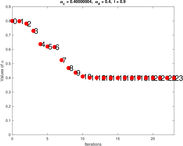
Figure 14: Test 8, identification of $\alpha$, $\ell=0.9$.

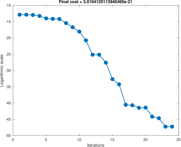
Figure 15: Test 8, current function values.

5.3.2 Strong degeneracy I

Test 9

Let us consider the strong degeneracy case with $1\leq\alpha<2$, i.e. the problem (17). We take $\alpha_{i}=1.6$ and $\alpha_{d}=1.3$. The numerical results can be seen in the Figures 17 and 17. In the Table 9, we present the computed values of $\alpha_{c}$ depending on the values of $\ell$ close to 1.

Table 9: Computed $\alpha_{c}$ for $\ell$ close to 1 in Test 9.

$\ell$	Cost	Iterations	$\alpha_{c}$	$\ell$	Cost	Iterations	$\alpha_{c}$
0.9	1.e-24	18	1.3	1.00001	1.e-22	23	1.30000001
0.99	1.e-22	24	1.30000001	1.0001	1.e-23	21	1.3
0.999	1.e-21	19	1.30000006	1.001	1.e-23	25	1.3
0.9999	1.e-23	22	1.29999999	1.01	1.e-24	32	1.3
0.99999	1.e-22	30	1.30000001	1.1	1.e-22	18	1.29999998
1	1.e-23	27	1.30000000	1.2	1.e-22	20	1.3

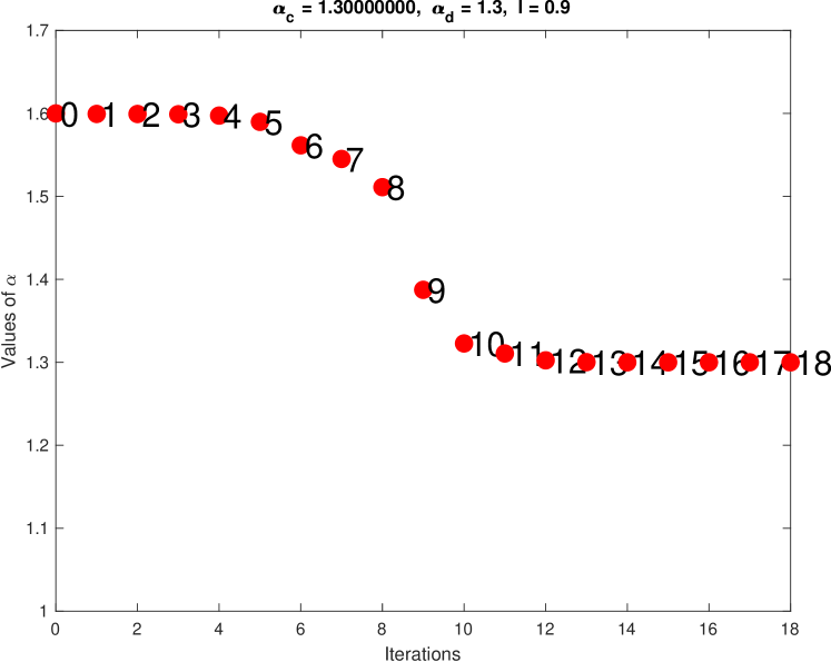
Figure 16: Test 9, identification of $\alpha$, $\ell=0.9$.

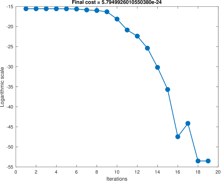
Figure 17: Test 9, current function values.

Remark 5.2

From the results of the Tests 8 and 9 we can see numerically that the hypothesis $\ell<1$ from Theorem 3.7 probably is not really needed for the reconstruction of $\alpha$. But the question whether we can eliminate this condition form this theorem remains open.

5.4 Numerical tests for the power-like case II

We will present in this section numerical results for the reconstruction of $\alpha$ from one observation of the form $\partial_{x}u(1,t)$. As before, we will analyze first weak and then strong degenerate cases. More precisely, given $\ell$, $u_{0}=u_{0}(x)$ and $\eta=\partial_{x}u(1,\cdot)$, we will solve numerically the following optimization problem (70), but wiht the functional $J:(0,2)\mapsto\mathds{R}$ given by

$$J(\alpha)=\dfrac{1}{2}\displaystyle\int_{0}^{T}|\eta(t)-\partial_{x}u^{\alpha}(1,t)|^{2}\,dt,$$

where $u^{\alpha}$ is the solution to (16) or (17) corresponding to $\alpha$.

In that follows, we will take $T=10$, $\ell=1$, $u_{0}=0.3x^{2}(1-x)^{2}$ and $f(x,t)=0$. The computations are performed using fmincon MatLab function form the Optimization Toolbox, combined with interior-point gradient algorithm.

5.4.1 Weak degeneracy II

Test 10

Let us first consider the weak degeneracy case corresponding to the problem (16) with $0<\alpha<1$. We take $\alpha_{i}=0.2$ as an initial guess for the minimization algorithm and the desired value to recover $\alpha_{d}=0.6$. The numerical results can be seen in Figures 19 and 19. Table 5.4.1 shows the computations of $\alpha_{c}$ and the cost with random noises in the target.

Figure 18: Test 10, identification of $\alpha$.

Figure 19: Test 10, current function values.

Table 10: Evolution of the cost and computed $\alpha_{c}$ with random noises in the target in Test 10.

% noise	Cost	Iterations	$\alpha_{c}$
1%	1.e-8	15	0.59689497
0.1%	1.e-10	16	0.60037182
0.01%	1.e-12	16	0.59997672
0.001%	1.e-14	18	0.59999807
0%	1.e-21	17	0.6

Figure 20: Test 10, order of convergence.

Remark 5.3 (On the order of convergence)

We can analyze the order of convergence of $\alpha_{n}$ which we obtain at each iteration $n$ of the optimization algorithm to $\alpha_{d}$. More precisely, we look for positive real numbers $C$ and $\kappa$ such that

$$|e_{n+1}|\approx C|e_{n}|^{\kappa},$$

where $e_{n}=\alpha_{n}-\alpha_{d}$. From Figure 20, we see that this approximate formula is satisfied for $\kappa=1.8$ for some finite value of $C$.

5.4.2 Strong degeneracy II

We will consider here the identification of $\alpha$ in the case $1\leq\alpha<2$ for strong degeneracy case, that is to say for the problem (17). For simplicity of the presentation, the results with random noises in the targets are not presented, because they are similar to those of the previous sections.

Test 11

Let us take $\ell=0.99$ and $\alpha_{i}=1.6$ as an initial guess for the minimization algorithm. The desired value of $\alpha$ to recover is $\alpha_{d}=1.3$. The numerical results can be seen in the Figures 24 and 24 and the computed value of $\alpha$ is $\alpha_{c}=1.3$.

Figure 21: Test 12, identification of $\alpha$.

Figure 22: Test 12, current function values.

Test 12

Let us take $\ell=1$ and $\alpha_{i}=1.6$ and $\alpha_{d}=1.3$. The numerical results can be seen in Figures 24 and 24 and the computed value is $\alpha_{c}=1.3$.

Figure 23: Test 12, identification of $\alpha$.

Figure 24: Test 12, current function values.

5.5 Numerical tests for a general case

In this section we will present numerical results of identification of a function $a=a(x)$ in (25) from $\partial_{x}u(1,t)$ in order to illustrate the theoretical part form the Section 4.

Let us take $\ell=1$, $T=5$, $\alpha=0.6$ and $u_{0}(x)=0.3x^{2}(1-x)^{2}$. In order to reconstruct $a=a(x)$, again we reformulate the corresponding inverse problem as an optimization problem: find $a\in\mathcal{A}$ such that

$$J(a)\leq J(a^{\prime}),\quad\forall\,a^{\prime}\in\mathcal{A}\,,$$ (71)

where the functional $J:\mathcal{A}\mapsto\mathds{R}$ is given by

$$J(a)=\dfrac{1}{2}\displaystyle\int_{0}^{T}|\eta(t)-\partial_{x}u^{a}(1,t)|^{2}\,dt,$$

where $u^{a}$ is the solution of (25) corresponding to $a$ and $\mathcal{A}$ is given by (27). In fact, for the numerical reconstruction we do not need to assume that $a$ is known near 1 as in (27).

In order to present some examples, in what follows we will analyze two particular cases of the coefficient $a(x)$: linear and quadratic functions. The numerical experiments will be performed using a gradient based interior-point algorithm of fmincon MatLab Optimization Toolbox.

Let us notice that we can also reconstruct numerically both $\alpha$ and $a$ from one measurement, but in order to simplify the presentations of the results, we will omit the details.

Linear function:

Let us consider $a$ of the form $a(x)=bx+c$, where $b$ and $c$ are unknown constants. The optimization problem (71) is written in this case as follows: find $b,c\in\mathcal{A}$, with $\mathcal{A}=\{(b,c):0<\underline{b}<b<\overline{b},\quad 0<\underline{c}<c<\overline{c}\}$ such that

$$J(b,c)\leq J(b^{\prime},c^{\prime}),\quad\forall\,(b^{\prime},c^{\prime})\in\mathcal{A}.$$

Test 13

Let us take $b_{i}=1$ and $c_{i}=1$ as initial guess for the optimization algorithm and desired values to recover $b_{d}=5$ and $c_{d}=1.5$. After numerical approximation of the optimization problem above we get the computed values $b_{c}=5$ and $c_{c}=1.5$. The numerical results we have obtained are in Figures 26 and 26. Table 5.5 shows the evolution of the cost during the iterations of optimization algorithm and computed $b_{c}$ and $c_{c}$ with random noises in the target. Finally, in Figure 27 the solution of (25) is represented for the computed values of the coefficients.

Figure 25: Test 13, $a_{d}$ solid line, $a_{c}$ dashed line.

Figure 26: Test 13, evolution of the cost.

Table 11: Evolution of the cost and computed $b_{c}$ and $c_{c}$ with random noises in the target in Test 13.

%	Cost	It.	$b_{c}$	$c_{c}$
1	1.e-8	29	5.02223088	1.47406114
0.1	1.e-10	29	5.00636935	1.49523326
0.01	1.e-12	29	4.99989752	1.50032299
0.001	1.e-14	29	4.99994089	1.50011971
0	1.e-25	39	5	1.5

Figure 27: Test 13, computed solution.

Quadratic function:

Let us now consider $a$ of the form $a(x)=bx^{2}+cx+h$. The optimization problem (71) is written in this case as follows: find $(b,c,h)\in\mathcal{A}$, with $\mathcal{A}=\{(b,c,h):0<\underline{b}<b<\overline{b},\quad 0<\underline{c}<c<\overline{c},\quad 0<\underline{h}<h<\overline{h}\}$ such that

$$J(b,c,h)\leq J(b^{\prime},c^{\prime},h^{\prime}),\quad\forall\,(b^{\prime},c^{\prime},h^{\prime})\in\mathcal{A}.$$

Test 14

Let us take $b_{i}=3.5$, $c_{i}=2.5$ and $h_{i}=0.5$ as initial guess for the optimization algorithm and the desired values to recover $b_{d}=4$, $c_{d}=3$ and $h_{d}=1$. The numerical results are shown in the Figures 29 and 29, and the computed values are $b_{c}=4.06562197$, $c_{c}=2.88613622$ and $h_{c}=1.04967427$. The numerical results can be seen in Figures 29 and 29. Table 5.5 shows the evolution of the cost during the iterations of optimization algorithm and computed $b_{c}$ and $c_{c}$ with random noises in the target.

Figure 28: Test 14, $a_{d}$ solid, $a_{c}$ dashed lines.

Figure 29: Test 14, evolution of the cost.

Table 12: Evolution of the cost and computed $b_{c}$ and $c_{c}$ with random noises in the target in Test 14.

%	Cost	Iterations	$b_{c}$	$c_{c}$	$h_{c}$
1%	1.e-8	41	4.05971241	2.88655292	1.09105166
0.1%	1.e-10	33	4.06806662	2.88685441	1.04274887
0.01%	1.e-12	34	4.06565361	2.88623199	1.05038351
0.001%	1.e-12	35	4.06567662	2.88615326	1.04953132
0%	1.e-12	33	4.06562197	2.88613622	1.04967427

References

- [1] F. Alabau-Boussouira, P. Cannarsa, G. Leugering, Control and stabilization of degenerate wave equations, SIAM J. Control and Optim. 55 (2017) 2052-2087.
- [2] J. Apraiz, J. Cheng, A. Doubova, E. Fernández-Cara, M. Yamamoto, Uniqueness and numerical reconstruction for inverse problems dealing wit interval size search, submitted.
- [3] R. Aster, B. Borchers, C. Thurber, Parameter estimation and inverse problems, Amsterdam, Elsevier, 2019.
- [4] M. Bellassoued, M. Yamamoto, Carleman Estimates and Applications to Inverse Problems for Hyperbolic Systems, Springer-Japan, Tokyo, 2017.
- [5] F. Black and M. Scholes, The pricing of options and corporate liabilities, J. Polit. Econ., 81 (1973), pp. 637-654.
- [6] A.L. Bukhgeim, M.V.Klibanov, Global uniqueness of class of multidimentional inverse problems, Soviet Math. Dokl. 24 (1981) 244-247.
- [7] P. Cannarsa, P. Martinez, J. Vancostenoble, Global Carleman estimates for degenerate parabolic operators with applications, Mem. Amer. Math. Soc. 239 (2016), no. 1133.
- [8] P. Cannarsa, J. Tort, M. Yamamoto, Determination of source terms in a degenerate parabolic equation, Inverse Problems 26 (2010), no. 10.
- [9] G. Citti, M. Manfredini, A degenerate parabolic equation arising in image processing, Commun. Appl. Anal., 8 (2004), pp. 125-141.
- [10] Z.-C. Deng, K. Qian, X.-B. Rao, L. Yang, G.-W. Luo, An inverse problem of identifying the source coefficient in a degenerate heat equation, Inverse Probl. Sci. Eng. 23 (2015), no. 3, 498–517.
- [11] Z.-C. Deng, L. Yang, An inverse problem of identifying the coefficient of first-order in a degenerate parabolic equation, J. Comput. Appl. Math. 235 (2011), no. 15, 4404–4417.
- [12] J. I. Díaz, ed., The Mathematics of Models for Climatology and Environment, NATO Adv. Sci. Inst. Ser. I: Global Environ. Change 48, Springer, Berlin, 1997.
- [13] A. Doubova, E. Fernández-Cara, Some geometric inverse problems for the linear wave equation, Inverse Probl. Imaging 9 (2015), no. 2, 371-393.
- [14] S.N. Ethier, A class of degenerate diffusion processes occurring in population genetics, Comm. Pure Appl. Math., 29 (1976), pp. 483-493.
- [15] S. Ji, R. Huang, On the Budyko-Sellers climate model with mushy region, J. Math. Anal. Appl. 434 (2016), no. 1, 581-598.
- [16] J. Hadamard, Sur les problèmes aux dérivées partielles et leur signification physique, Princeton University Bulletin, (1902), 49–52.
- [17] X. Huang, O.Y. Imanuvilov, M. Yamamoto, Stability for inverse source problems by Carleman estimates, Inverse Problems 36 (2020) 125006, 20 pp.
- [18] M.S. Hussein, D. Lesnic, V.L. Kamynin, A.B. Kostin, Direct and inverse source problems for degenerate parabolic equations, J. Inverse Ill-Posed Probl. 28 (2020), no. 3, 425–448.
- [19] O.Y. Imanuvilov, On Carleman estimates for hyperbolic equations, Asymptotic Anal. 32 (2002) 185-220.
- [20] O. Imanuvilov and M. Yamamoto, Lipschitz stability in inverse parabolic problems by the Carleman estimate, Inverse Problems 14 (1998) 1229-1245.
- [21] O. Imanuvilov, M. Yamamoto, Global Lipschitz stability in an inverse hyperbolic problem by interior observations, Inverse Problems 17 (2001) 717-728.
- [22] O.Y. Imanuvilov, M. Yamamoto, Determination of a coefficient in an acoustic equation with a single measurement, Inverse Problems 19 (2003) 157-171.
- [23] V. Isakov, Inverse Problems for Partial Differential Equations, Springer-Verlag, Berlin, 2006.
- [24] S. Ji, R. Huang, On the Budyko-Sellers climate model with mushy region, J. Math. Anal. Appl. 434 (2016), no. 1, 581-598.
- [25] V.L. Kamynin, Inverse problem of determining the absorption coefficient in a degenerate parabolic equation in the class of -functions, J. Math. Sci. (N.Y.) 250 (2020), no. 2, Problems in mathematical analysis. No. 105, 121–133.
- [26] M.V. Klibanov, Inverse problems and Carleman estimates, Inverse Problems 8 (1992) 575-596.
- [27] M.V. Klibanov, A. Timonov, Carleman Estimates for Coefficient Inverse Problems and Numerical Applications, VSP, Utrecht, 2004.
- [28] M. Kern, Numerical methods for inverse problems, ISTE, London; John Wiley & Sons, Inc., Hoboken, NJ, 2016.
- [29] M.M. Lavrentiev, A.V. Avdeev, M.M. Lavrentiev Jr., V.I. Priimenko, Inverse problems of mathematical physics, Inverse and Ill-posed Problems Series. VSP, Utrecht, 2003.
- [30] P. Martinez, J. Vancostenoble, Carleman estimates for one-dimensional degenerate heat equations, J. Evol. Equ. 6 (2006), no. 2, 325-362.
- [31] R. Murayama, The Gel’fand-Levitan theory and certain inverse problems for the parabolic equation, J. Fac. Sci. The Univ. Tokyo Section IA, Math. 28 (1981) 317–330.
- [32] O. A. Oleinik, V. N. Samokhin, Mathematical models in boundary layer theory, Applied Mathematics and Mathematical Computation, vol. 15, Chapman & Hall/CRC, Boca Raton, FL, 1999.
- [33] A. Pierce, Unique identification of eigenvalues and coefficients in a parabolic problem, SIAM J. Control and Optim. 17 (1979) 494–499.
- [34] V.G. Romanov, Inverse Problems of Mathematical Physics, VNU, Utrecht, 1987.
- [35] A.A. Samarskii, P.N. Vabishchevich, Numerical methods for solving inverse problems of mathematical physics, Inverse and Ill-posed Problems Series, 52. Walter de Gruyter GmbH & Co. KG, Berlin, 2007.
- [36] W. D. Sellers, A climate model based on the energy balance of the earth-atmosphere system, J. Appl. Meteor., 8 (1969), pp. 392-400.
- [37] T. Suzuki and R. Murayama, A uniqueness theorem in an identification problem for coefficients of parabolic equations, Proc. Japan Acad. Ser. A 56 (1980) 259–263.
- [38] C. R. Vogel, Computational methods for inverse problems, SIAM, Philadelphia, PA, 2002.
- [39] J. Tort, Determination of source terms in a degenerate parabolic equation from a locally distributed observation, C. R. Math. Acad. Sci. Paris 348 (2010), no. 23-24, 1287–1291.
- [40] J. Tort, An inverse diffusion problem in a degenerate parabolic equation, A special tribute to Professor Monique Madaune-Tort, 137–145, Monogr. Real Acad. Ci. Exact. Fís.-Quím. Nat. Zaragoza, 38, 2012.
- [41] M. Yamamoto, Carleman estimates for parabolic equations and applications, Inverse Problems 25 (2009) 123013.