Entropy-based Logic Explanations of Neural Networks

Entropy-based Logic Explanations of Neural Networks

Abstract

Explainable artificial intelligence has rapidly emerged since lawmakers have started requiring interpretable models for safety-critical domains. Concept-based neural networks have arisen as explainable-by-design methods as they leverage human-understandable symbols (i.e. concepts) to predict class memberships. However, most of these approaches focus on the identification of the most relevant concepts but do not provide concise, formal explanations of how such concepts are leveraged by the classifier to make predictions. In this paper, we propose a novel end-to-end differentiable approach enabling the extraction of logic explanations from neural networks using the formalism of First-Order Logic. The method relies on an entropy-based criterion which automatically identifies the most relevant concepts. We consider four different case studies to demonstrate that: (i) this entropy-based criterion enables the distillation of concise logic explanations in safety-critical domains from clinical data to computer vision; (ii) the proposed approach outperforms state-of-the-art white-box models in terms of classification accuracy and matches black box performances.

1 Introduction

The lack of transparency in the decision process of some machine learning models, such as neural networks, limits their application in many safety-critical domains (EUGDPR 2017; Goddard 2017). For this reason, explainable artificial intelligence (XAI) research has focused either on explaining black box decisions (Zilke, Loza Mencía, and Janssen 2016; Ying et al. 2019; Ciravegna et al. 2020a; Arrieta et al. 2020) or on developing machine learning models interpretable by design (Schmidt and Lipson 2009; Letham et al. 2015; Cranmer et al. 2019; Molnar 2020). However, while interpretable models engender trust in their predictions (Doshi-Velez and Kim 2017, 2018; Ahmad, Eckert, and Teredesai 2018; Rudin et al. 2021), black box models, such as neural networks, are the ones that provide state-of-the-art task performances (Battaglia et al. 2018; Devlin et al. 2018; Dosovitskiy et al. 2020; Xie et al. 2020). Research to address this imbalance is needed for the deployment of cutting-edge technologies.

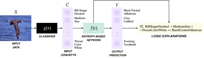
Figure 1: The proposed pipeline on one example from the CUB dataset. The neural network $f\colon C\mapsto Y$ maps concepts onto target classes and provide concise logic explanations (yellow – arguments of predicates are dropped for simplicity) of its own decision process. When the input data is non-interpretable (as pixels intensities), a classifier $g\colon X\mapsto C$ maps inputs to concepts.

Most techniques explaining black boxes focus on finding or ranking the most relevant features used by the model to make predictions (Simonyan, Vedaldi, and Zisserman 2013; Zeiler and Fergus 2014; Ribeiro, Singh, and Guestrin 2016b; Lundberg and Lee 2017; Selvaraju et al. 2017). Such feature-scoring methods are very efficient and widely used, but they cannot explain how neural networks compose such features to make predictions (Kindermans et al. 2019; Kim et al. 2018b; Alvarez-Melis and Jaakkola 2018). In addition, a key issue of most explaining methods is that explanations are given in terms of input features (e.g. pixel intensities) that do not correspond to high-level categories that humans can easily understand (Kim et al. 2018b; Su, Vargas, and Sakurai 2019). To overcome this issue, concept-based approaches have become increasingly popular as they provide explanations in terms of human-understandable categories (i.e. the concepts) rather than raw features (Kim et al. 2018b; Ghorbani et al. 2019; Koh et al. 2020; Chen, Bei, and Rudin 2020). However, fewer approaches are able to explain how such concepts are leveraged by the classifier and even fewer provide concise explanations whose validity can be assessed quantitatively (Ribeiro, Singh, and Guestrin 2016b; Guidotti et al. 2018; Das and Rad 2020).

Contributions. In this paper, we first propose an entropy-based layer (Sec. 3.1) that enables the implementation of concept-based neural networks, providing First-Order Logic explanations (Fig. 1). The proposed approach is not just a post-hoc method, but an explainable by design approach as it embeds additional constraints both in the architecture and in the learning process, to allow the emergence of simple logic explanations. This point of view is in contrast with post-hoc methods, which generally do not impose any constraint on classifiers: After the training is completed, the post-hoc method kicks in. Second, we describe how to interpret the predictions of the proposed neural model to distill logic explanations for individual observations and for a whole target class (Sec. 3.3). We demonstrate how the proposed approach provides high-quality explanations according to six quantitative metrics while matching black-box and outperforming state-of-the-art white-box models (Sec. 4) in terms of classification accuracy on four case studies (Sec. 5). Finally, we share an implementation of the entropy layer, with extensive documentation and all the experiments in the public repository: https://github.com/pietrobarbiero/entropy-lens.

2 Background

Classification is the problem of identifying a set of categories an observation belongs to. We indicate with $Y\subset\{0,1\}^{r}$ the space of binary encoded targets in a problem with $r$ categories. Concept-based classifiers $f$ are a family of machine learning models predicting class memberships from the activation scores of $k$ human-understandable categories, $f:C\mapsto Y$, where $C\subset[0,1]^{k}$ (see Fig. 1). Concept-based classifiers improve human understanding as their input and output spaces consists of interpretable symbols. When observations are represented in terms of non-interpretable input features belonging to $X\subset\mathbb{R}^{d}$ (such as pixels intensities), a “concept decoder” $g$ is used to map the input into a concept-based space, $g:X\mapsto C$ (see Fig. 1). Otherwise, they are simply rescaled from the unbounded space $\mathbb{R}^{d}$ into the unit interval $[0,1]^{k}$, such that input features can be treated as logic predicates.

In the recent literature, the most similar method related to the proposed approach is the $\psi$ network proposed by Ciravegna et al. (Ciravegna et al. 2020a, b), an end-to-end differentiable concept-based classifier explaining its own decision process. The $\psi$ network leverages the intermediate symbolic layer whose output belongs to $C$ to distill First-Order Logic formulas, representing the learned map from $C$ to $Y$. The model consists of a sequence of fully connected layers with sigmoid activations only. An $L1$-regularization and a strong pruning strategy is applied to each layer of weights in order to allow the computation of logic formulas representing the activation of each node. Such constraints, however, limit the learning capacity of the network and impair the classification accuracy, making standard white-box models, such as decision trees, more attractive.

3 Entropy-based Logic Explanations of Neural Networks

The key contribution of this paper is a novel linear layer enabling entropy-based logic explanations of neural networks (see Fig. 2 and Fig. 3). The layer input belongs to the concept space $C$ and the outcomes of the layer computations are: (i) the embeddings $h^{i}$ (as any linear layer), (ii) a truth table $\mathcal{T}^{i}$ explaining how the network leveraged concepts to make predictions for the $i$-th target class. Each class of the problem requires an independent entropy-based layer, as emphasized by the superscript $i$. For ease of reading and without loss of generality, all the following descriptions concern inference for a single observation (corresponding to the concept tuple $c\in C$) and a neural network $f^{i}$ predicting the class memberships for the $i$-th class of the problem. For multi-class problems, multiple “heads” of this layer are instantiated, with one “head” per target class (see Sec. 5), and the hidden layers of the class-specific networks could be eventually shared.

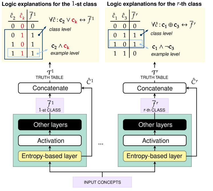
Figure 2: For each class $i$, the network leverages one “head” of the entropy-based linear layer (green) as first layer, and it provides: the class membership predictions $f^{i}$ and the truth table $\mathcal{T}^{i}$ (Eq. 6) to distill FOL explanations (yellow, top).

3.1 Entropy-based linear layer

When humans compare a set of hypotheses outlining the same outcomes, they tend to have an implicit bias towards the simplest ones as outlined in philosophy (Soklakov 2002; Rathmanner and Hutter 2011), psychology (Miller 1956; Cowan 2001), and decision making (Simon 1956, 1957, 1979). The proposed entropy-based approach encodes this inductive bias in an end-to-end differentiable model. The purpose of the entropy-based linear layer is to encourage the neural model to pick a limited subset of input concepts, allowing it to provide concise explanations of its predictions. The learnable parameters of the layer are the usual weight matrix $W$ and bias vector $b$. In the following, the forward pass is described by the operations going from Eq. 1 to Eq. 4 while the generation of the truth tables from which explanations are extracted is formalized by Eq. 5 and Eq. 6.

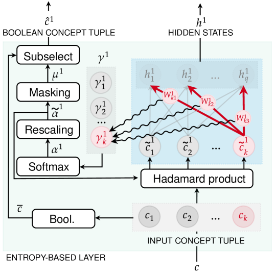
Figure 3: A detailed view on one “head” of the entropy-based linear layer for the $1$-st class, emphasizing the role of the $k$-th input concept as example: (i) the scalar $\gamma_{k}^{1}$ (Eq. 1) is computed from the set of weights connecting the $k$-th input concept to the output neurons of the entropy-based layer; (ii) the relative importance of each concept is summarized by the categorical distribution $\alpha^{1}$ (Eq. 2); (iii) rescaled relevance scores $\tilde{\alpha}^{1}$ drop irrelevant input concepts out (Eq. 3); (iv) hidden states $h^{1}$ (Eq. 4) and Boolean-like concepts $\hat{c}^{1}$ (Eq. 5) are provided as outputs of the entropy-based layer.

The relevance of each input concept can be summarized in a first approximation by a measure that depends on the values of the weights connecting such concept to the upper network. In the case of network $f^{i}$ (i.e. predicting the $i$-th class) and of the $j$-th input concept, we indicate with $W_{j}^{i}$ the vector of weights departing from the $j$-th input (see Fig. 3), and we introduce

$$\gamma^{i}_{j}=||W^{i}_{j}||_{1}\ .$$ (1)

The higher $\gamma^{i}_{j}$, the higher the relevance of the concept $j$ for the network $f^{i}$. In the limit case ($\gamma_{j}^{i}\rightarrow 0$) the model $f^{i}$ drops the $j$-th concept out. To select only few relevant concepts for each target class, concepts are set up to compete against each other. To this aim, the relative importance of each concept to the $i$-th class is summarized in the categorical distribution $\alpha^{i}$, composed of coefficients $\alpha^{i}_{j}\in[0,1]$ (with $\sum_{j}\alpha_{j}^{i}=1$), modeled by the softmax function:

$$\alpha^{i}_{j}=\frac{e^{\gamma^{i}_{j}/\tau}}{\sum_{l=1}^{k}e^{\gamma^{i}_{l}/\tau}}$$ (2)

where $\tau\in\mathbb{R}^{+}$ is a user-defined temperature parameter to tune the softmax function. For a given set of $\gamma^{i}_{j}$, when using high temperature values ($\tau\rightarrow\infty$) all concepts have nearly the same relevance. For low temperatures values ($\tau\rightarrow 0$), the probability of the most relevant concept tends to $\alpha_{j}^{i}\approx 1$, while it becomes $\alpha_{k}^{i}\approx 0,\ k\neq j$, for all other concepts. For further details on the impact of $\tau$ on the model predictions and explanations, see Appendix A.6. As the probability distribution $\alpha^{i}$ highlights the most relevant concepts, this information is directly fed back to the input, weighting concepts by the estimated importance. To avoid numerical cancellation due to values in $\alpha^{i}$ close to zero, especially when the input dimensionality is large, we replace $\alpha^{i}$ with its normalized instance $\tilde{\alpha}^{i}$, still in $[0,1]^{k}$, and each input sample $c\in C$ is modulated by this estimated importance,

$$\tilde{c}^{i}=c\odot\tilde{\alpha}^{i}\qquad\qquad\text{with}\qquad\tilde{\alpha}_{j}^{i}=\frac{\alpha_{j}^{i}}{\max_{u}\alpha_{u}^{i}},$$ (3)

where $\odot$ denotes the Hadamard (element-wise) product. The highest value in $\tilde{\alpha}^{i}$ is always $1$ (i.e. $\max_{j}\tilde{\alpha}_{j}^{i}=1$) and it corresponds to the most relevant concept. The embeddings $h^{i}$ are computed as in any linear layer by means of the affine transformation:

$$h^{i}=W^{i}\tilde{c}^{i}+b^{i}.$$ (4)

Whenever $\tilde{\alpha}_{j}^{i}\rightarrow 0$, the input $\tilde{c}_{j}^{i}\rightarrow 0$. This means that the corresponding concept tends to be dropped out and the network $f^{i}$ will learn to predict the $i$-th class without relying on the $j$-th concept.

In order to get logic explanations, the proposed linear layer generates the truth table $\mathcal{T}^{i}$ formally representing the behaviour of the neural network in terms of Boolean-like representations of the input concepts. In detail, we indicate with $\bar{c}$ the Boolean interpretation of the input tuple $c\in C$, while $\mu^{i}\in\{0,1\}^{k}$ is the binary mask associated to $\tilde{\alpha}^{i}$. To encode the inductive human bias towards simple explanations (Miller 1956; Cowan 2001; Ma, Husain, and Bays 2014), the mask $\mu^{i}$ is used to generate the binary concept tuple $\hat{c}^{i}$, dropping the least relevant concepts out of $c$,

$$\hat{c}^{i}=\xi(\bar{c},\mu^{i})\quad\text{with}\quad\mu^{i}=\mathbb{I}_{\tilde{\alpha}^{i}\geq{\color[rgb]{0,0,0}\epsilon}}\quad\text{and}\quad\bar{c}=\mathbb{I}_{c\geq{\color[rgb]{0,0,0}\epsilon}},$$ (5)

where $\mathbb{I}_{z\geq{\color[rgb]{0,0,0}\epsilon}}$ denotes the indicator function that is $1$ for all the components of vector $z$ being $\geq{\color[rgb]{0,0,0}\epsilon}$ and $0$ otherwise (considering the unbiased case, we set ${\color[rgb]{0,0,0}\epsilon}=0.5$). The function $\xi$ returns the vector with the components of $\bar{c}$ that correspond to $1$’s in $\mu^{i}$ (i.e. it sub-selects the data in $\bar{c}$). As a results, $\hat{c}^{i}$ belongs to a space $\hat{C}^{i}$ of $m_{i}$ Boolean features, with $m_{i}\textless k$ due to the effects of the subselection procedure.

The truth table $\mathcal{T}^{i}$ is a particular way of representing the behaviour of network $f^{i}$ based on the outcomes of processing multiple input samples collected in a generic dataset $\mathcal{C}$. As the truth table involves Boolean data, we denote with $\hat{\mathcal{C}}^{i}$ the set with the Boolean-like representations of the samples in $\mathcal{C}$ computed by $\xi$, Eq. 5. We also introduce $\bar{f}^{i}(c)$ as the Boolean-like representation of the network output, $\bar{f}^{i}(c)=\mathbb{I}_{f^{i}(c)\geq{\color[rgb]{0,0,0}\epsilon}}$. The truth table $\mathcal{T}^{i}$ is obtained by stacking data of $\hat{\mathcal{C}}^{i}$ into a 2D matrix $\hat{\mathbf{C}}^{i}$ (row-wise), and concatenating the result with the column vector $\bar{\mathbf{f}}^{i}$ whose elements are $\bar{f}^{i}(c)$, $c\in\mathcal{C}$, that we summarize as

$$\mathcal{T}^{i}=\Big{(}\hat{\mathbf{C}}^{i}\ \Big{|}\Big{|}\ \bar{\mathbf{f}}^{i}\Big{)}.$$ (6)

To be precise, any $\mathcal{T}^{i}$ is more like an empirical truth table than a classic one corresponding to an $n$-ary boolean function, indeed $\mathcal{T}^{i}$ can have repeated rows and missing Boolean tuple entries. However, $\mathcal{T}^{i}$ can be used to generate logic explanations in the same way, as we will explain in Sec. 3.3.

3.2 Loss function

The entropy of the probability distribution $\alpha^{i}$ (Eq. 2),

$$\mathcal{H}(\alpha^{i})=-\sum_{j=1}^{k}\alpha^{i}_{j}\log\alpha^{i}_{j}$$ (7)

is minimized when a single $\alpha^{i}_{j}$ is one, thus representing the extreme case in which only one concept matters, while it is maximum when all concepts are equally important. When $\mathcal{H}$ is jointly minimized with the usual loss function for supervised learning $L(f,y)$ (being $y$ the target labels–we used the cross-entropy in our experiments), it allows the model to find a trade off between fitting quality and a parsimonious activation of the concepts, allowing each network $f^{i}$ to predict $i$-th class memberships using few relevant concepts only. Overall, the loss function to train the network $f$ is defined as,

$$\mathcal{L}(f,y,\alpha_{1},\ldots,\alpha_{r})=L(f,y)+\lambda\sum_{i=1}^{r}\mathcal{H}(\alpha^{i}),$$ (8)

where $\lambda\textgreater 0$ is the hyperparameter used to balance the relative importance of low-entropy solutions in the loss function. Higher values of $\lambda$ lead to sparser configuration of $\alpha$, constraining the network to focus on a smaller set of concepts for each classification task (and vice versa), thus encoding the inductive human bias towards simple explanations (Miller 1956; Cowan 2001; Ma, Husain, and Bays 2014). For further details on the impact of $\lambda$ on the model predictions and explanations, see Appendix A.6. It may be pointed out that a similar regularization effect could be achieved by simply minimizing the $L_{1}$ norm over $\gamma^{i}$. However, as we observed in A.5, the $L_{1}$ loss does not sufficiently penalize the concept scores for those features which are uncorrelated with the predicted category. The Entropy loss, instead, correctly shrink to zero concept scores associated to uncorrelated features while the other remains close to one.

3.3 First-order logic explanations

Any Boolean function can be converted into a logic formula in Disjunctive Normal Form (DNF) by means of its truth-table (Mendelson 2009). Converting a truth table into a DNF formula provides an effective mechanism to extract logic rules of increasing complexity from individual observations to a whole class of samples. The following rule extraction mechanism is applied to any empirical truth table $\mathcal{T}^{i}$ for each task $i$.

FOL extraction.

Each row of the truth table $\mathcal{T}^{i}$ can be partitioned into two parts that are a tuple of binary concept activations, $\hat{q}\in\hat{C}^{i}$, and the outcome of $\bar{f}^{i}(\hat{q})\in\{0,1\}$. An example-level logic formula, consisting in a single minterm, can be trivially extracted from each row for which $\bar{f}^{i}(\hat{q})=1$, by simply connecting with the logic AND ($\wedge$) the true concepts and negated instances of the false ones. The logic formula becomes human understandable whenever concepts appearing in such a formula are replaced with human-interpretable strings that represent their name (similar consideration holds for $\bar{f}^{i}$, in what follows). For example, the following logic formula $\varphi^{i}_{t}$,

$$\varphi^{i}_{t}=\textbf{c}_{1}\wedge\ \neg\textbf{c}_{2}\wedge\ldots\wedge\textbf{c}_{m_{i}},$$ (9)

is the formula extracted from the $t$-th row of the table where, in the considered example, only the second concept is false, being $\textbf{c}_{z}$ the name of the $z$-th concept. Example-level formulas can be aggregated with the logic OR ($\vee$) to provide a class-level formula,

$$\bigvee_{t\in S_{i}}\varphi^{i}_{t},$$ (10)

being $S_{i}$ the set of rows indices of $\mathcal{T}^{i}$ for which $\bar{f}^{i}(\hat{q})=1$, i.e. it is the support of $\bar{f}^{i}$. We define with $\phi^{i}(\hat{c})$ the function that holds true whenever Eq. 10, evaluated on a given Boolean tuple $\hat{c}$, is true. Due to the aforementioned definition of support, we get the following class-level First-Order Logic (FOL) explanation for all the concept tuples,

$$\forall\hat{c}\in\hat{C}^{i}:\ \phi^{i}(\hat{c})\leftrightarrow\bar{f}^{i}(\hat{c}).$$ (11)

We note that in case of non-concept-like input features, we may still derive the FOL formula through the “concept decoder” function $g$ (see Sec. 2),

$$\forall x\in X:\ \phi^{i}\left(\xi(\overline{g(x)},\mu^{i})\right)\leftrightarrow\bar{f}^{i}\left(\xi(\overline{g(x)},\mu^{i})\right)$$ (12)

An example of the above scheme for both example and class-level explanations is depicted on top-right of Fig. 2.

Remarks.

The aggregation of many example-level explanations may increase the length and the complexity of the FOL formula being extracted for a whole class. However, existing techniques as the Quine–McCluskey algorithm can be used to get compact and simplified equivalent FOL expressions (McColl 1878; Quine 1952; McCluskey 1956). For instance, the explanation (person $\wedge$ nose) $\vee$ ($\neg$person $\wedge$ nose) can be formally simplified in nose. Moreover, the Boolean interpretation of concept tuples may generate colliding representations for different samples. For instance, the Boolean representation of the two samples $\{(0.1,0.7),(0.2,0.9)\}$ is the tuple $\bar{c}=(0,1)$ for both of them. This means that their example-level explanations match as well. However, a concept can be eventually split into multiple finer grain concepts to avoid collisions. Finally, we mention that the number of samples for which any example-level formula holds (i.e. the support of the formula) is used as a measure of the explanation importance. In practice, example-level formulas are ranked by support and iteratively aggregated to extract class-level explanations, until the aggregation improves the accuracy of the explanation over a validation set.

4 Related work

In order to provide explanations for a given black-box model, most methods focus on identifying or scoring the most relevant input features (Simonyan, Vedaldi, and Zisserman 2013; Zeiler and Fergus 2014; Ribeiro, Singh, and Guestrin 2016b, a; Lundberg and Lee 2017; Selvaraju et al. 2017). Feature scores are usually computed sample by sample (i.e. providing local explanations) analyzing the activation patterns in the hidden layers of neural networks (Simonyan, Vedaldi, and Zisserman 2013; Zeiler and Fergus 2014; Selvaraju et al. 2017) or by following a model-agnostic approach (Ribeiro, Singh, and Guestrin 2016a; Lundberg and Lee 2017). To enhance human understanding of feature scoring methods, concept-based approaches have been effectively employed for identifying common activations patterns in the last nodes of neural networks corresponding to human categories (Kim et al. 2018a; Kazhdan et al. 2020) or constraining the network to learn such concepts (Chen, Bei, and Rudin 2020; Koh et al. 2020). Either way, feature-scoring methods are not able to explain how neural networks compose features to make predictions (Kindermans et al. 2019; Kim et al. 2018b; Alvarez-Melis and Jaakkola 2018) and only a few of these approaches have been efficiently extended to provide explanations for a whole class (i.e. providing global explanations) (Simonyan, Vedaldi, and Zisserman 2013; Ribeiro, Singh, and Guestrin 2016a). By contrast, a variety of rule-based approaches have been proposed to provide concept-based explanations. Logic rules are used to explain how black boxes predict class memberships for indivudal samples (Guidotti et al. 2018; Ribeiro, Singh, and Guestrin 2018), or for a whole class (Sato and Tsukimoto 2001; Zilke, Loza Mencía, and Janssen 2016; Ciravegna et al. 2020a, b). Distilling explanations from an existing model, however, is not the only way to achieve explainability. Historically, standard machine-learning such as Logistic Regression (McKelvey and Zavoina 1975), Generalized Additive Models (Hastie and Tibshirani 1987; Lou, Caruana, and Gehrke 2012; Caruana et al. 2015) Decision Trees (Breiman et al. 1984; Quinlan 1986, 2014) and Decision Lists (Rivest 1987; Letham et al. 2015; Angelino et al. 2018) were devised to be intrinsically interpretable. However, most of them struggle in solving complex classification problems. Logistic Regression, for instance, in its vanilla definition, can only recognize linear patterns, e.g. it cannot to solve the XOR problem (Minsky and Papert 2017). Further, only Decision Trees and Decision Lists provide explanations in the from of logic rules. Considering decision trees, each path may be seen as a human comprehensible decision rule when the height of the tree is reasonably contained. Another family of concept-based XAI methods is represented by rule-mining algorithms which became popular at the end of the last century (Holte 1993; Cohen 1995). Recent research has led to powerful rule-mining approaches as Bayesian Rule Lists (BRL) (Letham et al. 2015), where a set of rules is “pre-mined” using the frequent-pattern tree mining algorithm (Han, Pei, and Yin 2000) and then the best rule set is identified with Bayesian statistics. In this paper, the proposed approach is compared with methods providing logic-based, global explanations. In particular, we selected one representative approach from different families of methods: Decision Trees (white-box machine learning), BRL (rule mining) and $\psi$ Networks (explainable neural models).

5 Experiments

The quality of the explanations and the classification performance of the proposed approach are quantitatively assessed and compared to state-of-the-art white-box models. A visual sketch of each classification problem (described in detail in Sec. 5.1) and a selection of the logic formulas found by the proposed approach is reported in Fig. 4. Six quantitative metrics are defined and used to compare the proposed approach with state-of-the-art methods. Sec. 5.2 summarizes the main findings. Further details concerning the experiments are reported in the supplemental material A.

Table 1: Classification accuracy (%). Left group, the compared white-box models. Right group, two black box models. We indicate in bold the best model in each group, with a star the best model overall.

	Entropy net	Tree	BRL	$\psi$ net	Neural Network	Random Forest
MIMIC-II	${\bf 79.05^{\star}\pm 1.35}$	$77.53\pm 1.45$	$76.40\pm 1.22$	$77.19\pm 1.64$	${\color[rgb]{0,0,0}77.81\pm 2.45}$	${\bf 78.88\pm 2.25}$
V-Dem	${\bf 94.51\pm 0.48}$	$85.61\pm 0.57$	$91.23\pm 0.75$	$89.77\pm 2.07$	${\color[rgb]{0,0,0}\bf 94.53^{\star}\pm 1.17}$	$93.08\pm 0.44$
MNIST	${\bf 99.81\pm 0.02}$	$99.75\pm 0.01$	$99.80\pm 0.02$	$99.79\pm 0.03$	${99.72\pm 0.03}$	${\bf 99.96^{\star}\pm 0.01}$
CUB	${\bf 92.95\pm 0.20}$	$81.62\pm 1.17$	$90.79\pm 0.34$	$91.92\pm 0.27$	${\bf{93.10}^{\star}\pm 0.51}$	$91.88\pm 0.36$

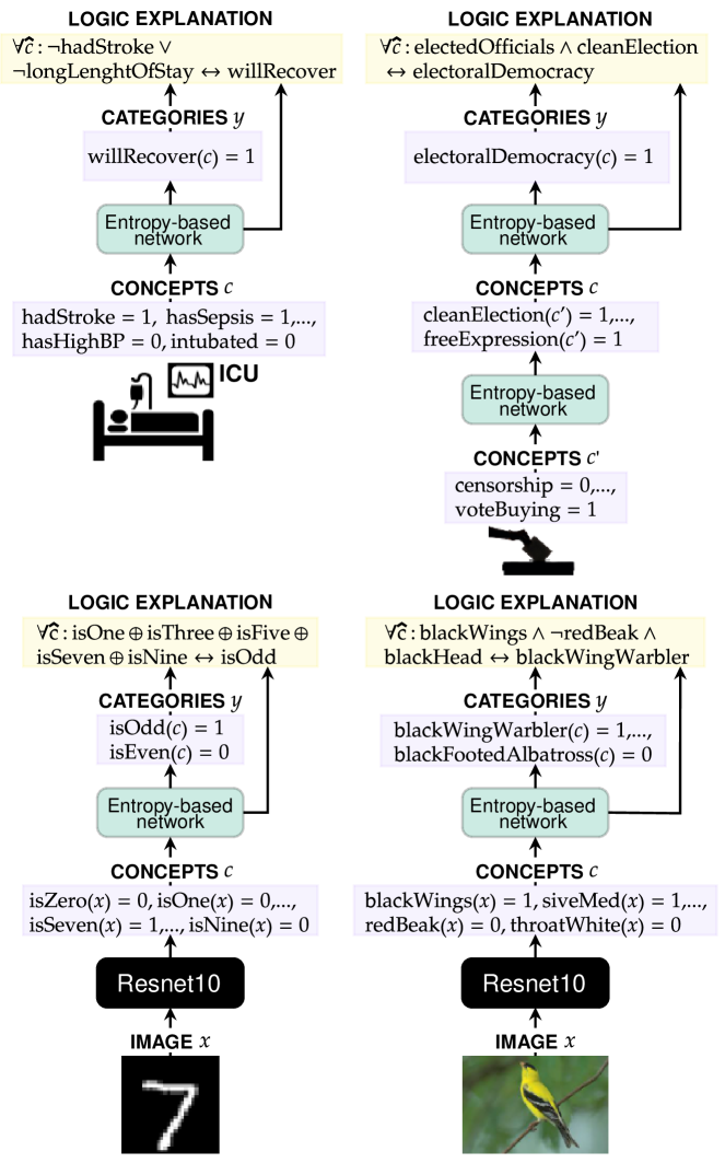
Figure 4: The four case studies show how the proposed Entropy-based networks (green) provide concise logic explanations (yellow) of their own decision process in different real-world contexts. When input features are non-interpretable, as pixel intensities, a “concept decoder” (ResNet10) maps images into concepts. Entropy-based networks then map concepts into target classes.

5.1 Classification tasks and datasets

Four classification problems ranging from computer vision to medicine are considered. Computer vision datasets (e.g. CUB) are annotated with low-level concepts (e.g. bird attributes) used to train concept bottleneck pipelines (Koh et al. 2020). In the other datasets, the input data is rescaled into a categorical space ($\mathbb{R}^{k}\rightarrow C$) suitable for concept-based networks. Please notice that this preprocessing step is performed for all white-box models considered in the experiments for a fair comparison. Further descriptions of each dataset and links to all sources are reported in Appendix A.2.
Will we recover from ICU? (MIMIC-II). The Multiparameter Intelligent Monitoring in Intensive Care II (MIMIC-II, (Saeed et al. 2011; Goldberger et al. 2000)) is a public-access intensive care unit (ICU) database consisting of 32,536 subjects (with 40,426 ICU admissions) admitted to different ICUs. The task consists in identifying recovering or dying patients after ICU admission. An end-to-end classifier $f:C\rightarrow Y$ carries out the classification task.
What kind of democracy are we living in? (V-Dem). Varieties of Democracy (V-Dem, (Pemstein et al. 2018; Coppedge et al. 2021)) dataset contains a collection of indicators of latent regime characteristics over 202 countries from 1789 to 2020. The database include $k_{1}=483$ low-level indicators $k_{2}=82$ mid-level indices. The task consists in identifying electoral democracies from non-electoral ones. We indicate with $C_{1}$, $C_{2}$ the spaces associated to the activations of the two levels of concepts. Classifiers $f_{1}$ and $f_{2}$ are trained to learn the map $C_{1}\rightarrow C_{2}\rightarrow Y$. Explanations are given for classifier $f_{2}$ in terms of concepts $c_{2}\in C_{2}$.
What does parity mean? (MNIST Even/Odd). The Modified National Institute of Standards and Technology database (MNIST, (LeCun 1998)) contains a large collection of images representing handwritten digits. The task we consider here is slightly different from the common digit-classification. Assuming $Y\subset\{0,1\}^{2}$, we are interested in determining if a digit is either odd or even, and explaining the assignment to one of these classes in terms of the digit labels (concepts in $C$). The mapping $X\rightarrow C$ is provided by a ResNet10 classifier $g$ (He et al. 2016) trained from scratch. while the classifier $f$ learn both the final mapping and the explanation as a function $C\rightarrow Y$.
What kind of bird is that? (CUB). The Caltech-UCSD Birds-200-2011 dataset (CUB, (Wah et al. 2011)) is a fine-grained classification dataset. It includes 11,788 images representing $r=200$ ($Y=\{0,1\}^{200}$) different bird species. 312 binary attributes (concepts in $C$) describe visual characteristics (color, pattern, shape) of particular parts (beak, wings, tail, etc.) for each bird image. The mapping $X\rightarrow C$ is performed with a ResNet10 model $g$ trained from scratch while the classifier $f$ learns the final function $C\rightarrow Y$.

Quantitative metrics.

Measuring the classification quality is of crucial importance for models that are going to be applied in real-world environments. On the other hand, assessing the quality of the explanations is required for a safedeployment. In contrast with other kind of explanations, logic-based formulas can be evaluated quantitatively. Given a classification problem, first a set of rules are extracted for each target category from each considered model. Each explanation is then tested on an unseen set of test samples. The results for each metric are reported in terms of mean and standard error, computed over a 5-fold cross validation (Krzywinski and Altman 2013). For each experiment and for each model model ($f:C\rightarrow Y$ mapping concepts to target categories) six quantitative metrics are measured. (i) The model accuracy measures how well the explainer identifies the target classes on unseen data (see Table 1). (ii) The explanation accuracy measures how well the extracted logic formulas identifies the target classes (Fig. 5). This metric is obtained as the average of the F1 scores computed for each class explanation. (iii) The complexity of an explanation is computed by standardizing the explanations in DNF and then by counting the number of terms of the standardized formula (Fig. 5): the longer the formula, the harder the interpretation for a human being. (iv) The fidelity of an explanation measures how well the extracted explanation matches the predictions obtained using the explainer (Table 2). (v) The rule extraction time measures the time required to obtain an explanation from scratch (see Fig. 6), computed as the sum of the time required to train the model and to extract the formula from a trained explainer. (vi) The consistency of an explanation measures the average similarity of the extracted explanations over the 5-fold cross validation runs (see Table 3), computed by counting how many times the same concepts appear in a logic formula over different iterations.

5.2 Results and discussion

Experiments show how entropy-based networks outperform state-of-the-art white box models such as BRL and decision trees and interpretable neural models such as $\psi$ networks on challenging classification tasks (Table 1). Moreover, the entropy-based regularization and the adoption of a concept-based neural network have minor affects on the classification accuracy of the explainer when compared to a standard black box neural network directly working on the input data, and a Random Forest model applied on the concepts.At the same time, the logic explanations provided by entropy-based networks are better than $\psi$ networks and almost as accurate as the rules found by decision trees and BRL, while being far more concise, as demonstrated in Fig. 5. More precisely, logic explanations generated by the proposed approach represent non-dominated solutions (Marler and Arora 2004) quantitatively measured in terms of complexity and classification error of the explanation. Furthermore, the time required to train entropy-based networks is only slightly higher with respect to Decision Trees but is lower than $\psi$ Networks and BRL by one to three orders of magnitude (Fig. 6), making it feasible for explaining also complex tasks. The fidelity (Table 2) of the formulas extracted by the entropy-based network is always higher than $90\%$ with the only exception of MIMIC. This means that almost any prediction made using the logic explanation matches the corresponding prediction made by the model, making the proposed approach very close to a white box model. The combination of these results empirically shows that our method represents a viable solution for a safe deployment of explainable cutting-edge models.

Table 2: Out-of-distribution fidelity (%)

	Entropy net	$\psi$ net
MIMIC-II	${\bf 79.11\pm 2.02}$	$51.63\pm 6.67$
V-Dem	${\bf 90.90\pm 1.23}$	$69.67\pm 10.43$
MNIST	${\bf 99.63\pm 0.00}$	$65.68\pm 5.05$
CUB	${\bf 99.86\pm 0.01}$	$77.34\pm 0.52$

Table 3: Consistency (%)

	Entropy net	Tree	BRL	$\psi$ net
MIMIC-II	$28.75$	${\bf 40.49}$	$30.48$	$27.62$
V-Dem	$46.25$	$72.00$	${\bf 73.33}$	$38.00$
MNIST	${\bf 100.00}$	$41.67$	${\bf 100.00}$	$96.00$
CUB	$35.52$	$21.47$	${\bf 42.86}$	$41.43$

The reason why the proposed approach consistently outperform $\psi$ networks across all the key metrics (i.e. classification accuracy, explanation accuracy, and fidelity) can be explained observing how entropy-based networks are far less constrained than $\psi$ networks, both in the architecture (our approach does not apply weight pruning) and in the loss function (our approach applies a regularization on the distributions $\alpha^{i}$ and not on all weight matrices). Likewise, the main reason why the proposed approach provides a higher classification accuracy with respect to BRL and decision trees may lie in the smoothness of the decision functions of neural networks which tend to generalize better than rule-based methods, as already observed by Tavares et al. (Tavares et al. 2020). For each dataset, we report in the supplemental material (Appendix A.7) a few examples of logic explanations extracted by each method, as well as in Fig. 4. We mention that the proposed approach is the only matching the logically correct ground-truth explanation for the MNIST even/odd experiment, i.e. $\forall x,\mathrm{isOdd(x)}\leftrightarrow\mathrm{isOne(x)}\oplus\mathrm{isThree(x)}\oplus\mathrm{isFive(x)}\oplus\mathrm{isSeven(x)}\oplus\mathrm{isNine(x)}$ and $\forall x,\mathrm{isEven(x)}\leftrightarrow\mathrm{isZero(x)}\oplus\mathrm{isTwo(x)}\oplus\mathrm{isfour(x)}\oplus\mathrm{isSix(x)}\oplus\mathrm{isEight(x)}$, being $\oplus$ the exclusive OR. In terms of formula consistency, we observe how BRL is the most consistent rule extractor, closely followed by the proposed approach (Table 3).

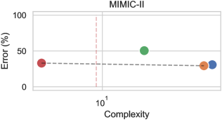
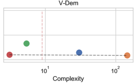
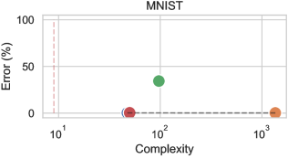
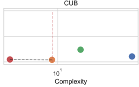
Figure 5: Non-dominated solutions (Marler and Arora 2004) (dotted black line) in terms of average explanation complexity and average explanation test error. The vertical dotted red line marks the maximum explanation complexity laypeople can handle (i.e. complexity $\approx 9$, see (Miller 1956; Cowan 2001; Ma, Husain, and Bays 2014)). Notice how the explanations provided by the Entropy-based Network are always one of the non-dominated solution.

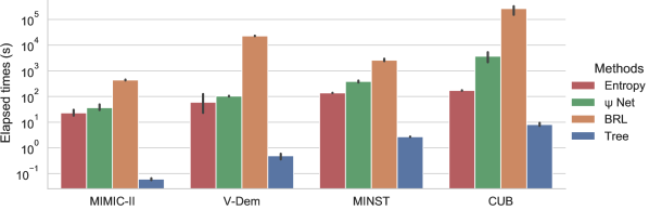
Figure 6: Time required to train models and to extract the explanations. Our model compares favorably with the competitors, with the exception of Decision Trees. BRL is by one to three order of magnitude slower than our approach.

6 Conclusions

This work contributes to a safer adoption of some of the most powerful AI technologies, allowing deep neural networks to have a greater impact on society by making them explainable-by-design, thanks to an entropy-based approach that yields FOL-based explanations. Moreover, as the proposed approach provides logic explanations for how a model arrives at a decision, it can be effectively used to reverse engineer algorithms, processes, to find vulnerabilities, or to improve system design powered by deep learning models. From a scientific perspective, formal knowledge distillation from state-of-the-art networks may enable scientific discoveries or falsification of existing theories. However, the extraction of a FOL explanation requires symbolic input and output spaces. In some contexts, such as computer vision, the use of concept-based approaches may require additional annotations and attribute labels to get a consistent symbolic layer of concepts. Recent works on automatic concept extraction may alleviate the related costs, leading to more cost-effective concept annotations (Ghorbani et al. 2019; Kazhdan et al. 2020).

Appendix A Appendix

A.1 Software

In order to make the proposed approach accessible to the whole community, we released Anonymous (Anonymous 2021), a Python package with an extensive documentation on methods and unit tests. The Python code and the scripts used for the experiments, including parameter values and documentation, is freely available under Apache 2.0 Public License from a GitHub repository.

The code library is designed with intuitive APIs requiring only a few lines of code to train and get explanations from the neural network as shown in the following code snippet 1.

⬇

1import torch_explain as te

2from torch_explain.logic import test_explanation

3from torch_explain.logic.nn import explain_class

4

5# XOR problem with additional features

6x0 = torch.zeros((4, 100))

7x = torch.tensor([

8 [0, 0, 0],

9 [0, 1, 0],

10 [1, 0, 0],

11 [1, 1, 0],

12], dtype=torch.float)

13x = torch.cat([x, x0], dim=1)

14y = torch.tensor([0, 1, 1, 0], dtype=torch.long)

15

16# network architecture

17layers = [

18 te.nn.EntropyLogicLayer(x.shape[1], 10, n_classes=2),

19 torch.nn.LeakyReLU(),

20 te.nn.LinearIndependent(10, 10, n_classes=2),

21 torch.nn.LeakyReLU(),

22 te.nn.LinearIndependent(10, 1, n_classes=2, top=True)

23]

24model = torch.nn.Sequential(*layers)

25

26# train loop

27optimizer = torch.optim.AdamW(model.parameters(), lr=0.01)

28loss_form = torch.nn.CrossEntropyLoss()

29model.train()

30for epoch in range(1001):

31 optimizer.zero_grad()

32 y_pred = model(x)

33 loss = loss_form(y_pred, y) + \

34 0.00001 * te.nn.functional.entropy_logic_loss(model)

35 loss.backward()

36 optimizer.step()

37

38# logic explanations

39y1h = one_hot(y)

40_, class_explanations, _ = explain_class(model, x, y1h, x, y1h)

Listing 1: Example on how to use the APIs to implement the proposed approach.

A.2 Dataset Description

Will we recover from ICU? (MIMIC-II).

The Multiparameter Intelligent Monitoring in Intensive Care II (MIMIC-II, (Saeed et al. 2011; Goldberger et al. 2000)) is a public-access intensive care unit (ICU) database consisting of 32,536 subjects (with 40,426 ICU admissions) admitted to different ICUs. The dataset contains detailed descriptions of a variety of clinical data classes: general, physiological, results of clinical laboratory tests, records of medications, fluid balance, and text reports of imaging studies (e.g. x-ray, CT, MRI, etc). In our experiments, we removed non-anonymous information, text-based features, time series inputs, and observations with missing data. We discretize continuous features into one-hot encoded categories. After such preprocessing step, we obtained an input space $C$ composed of $k=90$ key features. The task consists in identifying recovering or dying patients after ICU admission.

What kind of democracy are we living in? (V-Dem).

Varieties of Democracy (V-Dem, (Pemstein et al. 2018; Coppedge et al. 2021)) is a dataset containing a collection of indicators of latent regime characteristics over 202 countries from 1789 to 2020. The database include $k_{1}=483$ low-level indicators (e.g. media bias, party ban, high-court independence, etc.), $k_{2}=82$ mid-level indices (e.g. freedom of expression, freedom of association, equality before the law, etc), and 5 high-level indices of democracy principles (i.e. electoral, liberal, participatory, deliberative, and egalitarian). In the experiments a binary classification problem is considered to identify electoral democracies from non-electoral democracies. We indicate with $C_{1}$ and $C_{2}$ the spaces associated to the activations of the aforementioned two levels of concepts. Two classifiers $f_{1}$ and $f_{2}$ are trained to learn the map $C_{1}\rightarrow C_{2}\rightarrow Y$. Explanations are given for classifier $f_{2}$ in terms of concepts $c_{2}\in C_{2}$.

What does parity mean? (MNIST Even/Odd).

The Modified National Institute of Standards and Technology database (MNIST, (LeCun 1998)) contains a large collection of images representing handwritten digits. The input space $X\subset\mathbb{R}^{28\times 28}$ is composed of 28x28 pixel images while the concept space $C$ with $k=10$ is represented by the label indicator for digits from $0$ to $9$. The task we consider here is slightly different from the common digit-classification. Assuming $Y\subset\{0,1\}^{2}$, we are interested in determining if a digit is either odd or even, and explaining the assignment to one of these classes in terms of the digit labels (concepts in $C$). The mapping $X\rightarrow C$ is provided by a ResNet10 classifier $g$ (He et al. 2016) trained from scratch. while the classifier $f$ is used to learn both the final mapping and the explanation as a function $C\rightarrow Y$.

What kind of bird is that? (CUB).

The Caltech-UCSD Birds-200-2011 dataset (CUB, (Wah et al. 2011)) is a fine-grained classification dataset. It includes 11,788 images representing $r=200$ ($Y=\{0,1\}^{200}$) different bird species. 312 binary attributes describe visual characteristics (color, pattern, shape) of particular parts (beak, wings, tail, etc.) for each bird image. Attribute annotations, however, is quite noisy. For this reason, attributes are denoised by considering class-level annotations (Koh et al. 2020). In the end, a total of $108$ attributes (i.e. concepts with binary activations belonging to $C$) have been retained. The mapping $X\rightarrow C$ from images to attribute concepts is performed again with a ResNet10 model $g$ trained from scratch while the classifier $f$ learns the final function $C\rightarrow Y$.

All datasets employed are freely available (only MIMIC-II requires an online registration) and can be downloaded from the following links:
MIMIC: https://archive.physionet.org/mimic2.
V-Dem: https://www.v-dem.net/en/data/data/v-dem-dataset-v111.
MNIST: http://yann.lecun.com/exdb/mnist.
CUB: http://www.vision.caltech.edu/visipedia/CUB-200-2011.html.

A.3 Experimental details

Batch gradient-descent and the Adam optimizer with decoupled weight decay (Loshchilov and Hutter 2017) and learning rate set to $10^{-2}$ are used for the optimization of all neural models’ parameters (Entropy-based Network and $\psi$ Network). An early stopping strategy is also applied: the model with the highest accuracy on the validation set is saved and restored before evaluating the test set.

With regard to the Entropy-based Network, Tab. 4 reports the hyperparameters employed to train the network in all experiments. All Entropy-based Networks feature ReLU activations and linear fully-connected layers (except for the first layer which is the Entropy Layer). A grid search cross-validation strategy has been employed on the validation set to select hyperparameter values. The objective was to maximize at the same time both model and explanation accuracy. $\lambda$ represents the trade-off parameter in Eq. 8 while $\tau$ is the temperature of Eq. 2.

Table 4: Hyper parameters of entropy-based networks.

	$\lambda$	$\tau$	max epochs	hidden neurons
MIMIC-II	$10^{-3}$	$0.7$	200	$20$
V-Dem	$10^{-5}$	$5$	200	$20,20$
MNIST	$10^{-7}$	$5$	200	$10$
CUB	$10^{-4}$	$0.7$	500	$10$

Concerning the $\psi$ network in all experiments one network per class has been trained. They are composed of two hidden layer of 10 and 5 hidden neurons respectively. As indicated in the original paper, an $l_{1}$ weight regularization has been applied to all layers of the network. As in this work, the contribute in the overall loss of the $l_{1}$ regularization is weighted by an hyperparameter $\lambda=10^{-4}$. The maximum number of non-zero input weight (fan-in) is set to 3 in in MIMIC and V-Dem while for MNIST and CUB200 it is set to 4. In Ciravegna et al. (Ciravegna et al. 2020a), $\psi$ networks were devised to provide explanations of existing models; in this paper, however, we have shown how they can directly solve classification problems.

Decision Trees have been limited in their maximum height in all experiments to maintain the complexity of the rules at a comparable level w.r.t the other methods. More precisely the maximum height has been set to $5$ in all binary classification tasks (MIMIC-II, V-Dem, MNIST) while we allowed a maximum height of $30$ in the CUB experiment due to the high number of classes to predict (200).

BRL algorithms requires to first run the FP-growth algorithm (Han, Pei, and Yin 2000) (an enhanced version of Apriori) to mine a first set of frequent rules. The hyperparameter used by FP-growth are: the minimum support in percentage of training samples for each rule (set to $10\%$), the minimum and the maximum number of features considered by each rule (respectively set to 1 and 2). Regarding the Bayesian selection of the best rules, the number of Markov chain Monte Carlo used for inference is set to 3, while 50000 iterations maximum are allowed. At last the expected length and width of the extracted rule list is set respectively to 3 and 1. These are the default values indicated in the BRL repository. Due to the computational complexity and the high number of hyperparameters, they have not been cross validated.

The code for the experiments is implemented in Python 3, relying upon open-source libraries (Paszke et al. 2019; Pedregosa et al. 2011). All the experiments have been run on the same machine: Intel^® Core™ i7-10750H 6-Core Processor at 2.60 GHz equipped with 16 GiB RAM and NVIDIA GeForce RTX 2060 GPU.

A.4 Explainability metrics details

In the following, we report in tabular form the results concerning the explanation accuracy and the complexity of the rules (Fig. 5) and the extraction time (Fig. 6).

Table 5: Explanation’s accuracy (%) computed as the average of the F1 scores computed for each class.

	Entropy net	Tree	BRL	$\psi$ net
MIMIC-II	$66.93\pm 2.14$	$69.15\pm 2.24$	${\bf 70.59\pm 2.17}$	$49.51\pm 3.91$
V-Dem	$89.88\pm 0.50$	$85.45\pm 0.58$	${\bf 91.21\pm 0.75}$	$67.08\pm 9.68$
MNIST	$99.62\pm 0.00$	$99.74\pm 0.01$	${\bf 99.79\pm 0.02}$	$65.64\pm 5.05$
CUB	$95.24\pm 0.05$	$89.36\pm 0.92$	${\bf 96.02\pm 0.17}$	$76.10\pm 0.56$

Table 6: Complexity computed as the number of terms in each minterm of the DNF rules.

	Entropy net	Tree	BRL	$\psi$ net
MIMIC-II	${\bf 3.50\pm 0.88}$	$66.60\pm 1.45$	$57.70\pm 35.58$	$20.6\pm 5.36$
V-Dem	${\bf 3.10\pm 0.51}$	$30.20\pm 1.20$	$145.70\pm 57.93$	$5.40\pm 2.70$
MNIST	$50.00\pm 0.00$	${\bf 47.50\pm 0.72}$	$1352.30\pm 292.62$	$96.90\pm 10.01$
CUB	${\bf 3.74\pm 0.03}$	$45.92\pm 1.16$	$8.87\pm 0.11$	$15.96\pm 0.96$

Table 7: Rule extraction time (s) calculated as the time required to train the models and to extract the corresponding rules.

	Entropy net	Tree	BRL	$\psi$ net
MIMIC-II	$23.08\pm 3.53$	${\bf 0.06\pm 0.00}$	$440.24\pm 9.75$	$36.68\pm 6.10$
V-Dem	$59.90\pm 31.18$	${\bf 0.49\pm 0.07}$	$22843.21\pm 194.49$	$103.78\pm 1.65$
MNIST	$138.32\pm 0.63$	${\bf 2.72\pm 0.02}$	$2594.79\pm 177.34$	$385.57\pm 17.81$
CUB	$171.87\pm 1.95$	${\bf 8.10\pm 0.65}$	$264678.29\pm 56521.40$	$3707.29\pm 1006.54$

A.5 Entropy and L1

This section presents additional experiments on a toy dataset showing (1) the advantage of using the entropy loss function in Eq. 7 w.r.t. the L1 loss (used by e.g. the $\psi$ network) and (2) the advantage in terms of explainability provided by the Entropy Layer w.r.t. a standard linear layer. Three neural models are compared:

• model A: a standard multi-layer perceptron using linear (fully connected) layers, using an L1 regularization in the loss function.

• model B: a multi-layer perceptron using the Entropy Layer as first layer and an L1 regularization in the loss function.

• model C: a multi-layer perceptron using the Entropy Layer as first layer and the entropy loss regularization (Eq. 7) in the loss function.

The dataset used for this experiment is shown in Table 8. The training set is composed of four Boolean features $\{x_{1},x_{2},x_{3},x_{4}\}$ and four Boolean target categories $\{y,\neg y,z,\neg z\}$. The target category $y$ is the XOR of the features $x_{1}$ and $x_{2}$, i.e. $\forall x:y=1\leftrightarrow x_{1}\oplus x_{2}$. The target category $z$ is the OR of the features $x_{3}$ and $x_{4}$, i.e. $\forall x:z=1\leftrightarrow x_{3}\wedge x_{4}$. The categories $\neg y$ and $\neg z$ are the complement of the categories $y$ and $z$, respectively.

The neural networks used for these experiment are multi-layer perceptrons with 2 hidden layers of $20$ and $10$ units with ReLu activation. Batch gradient-descent and the Adam optimizer with decoupled weight decay (Loshchilov and Hutter 2017) and learning rate set to $10^{-4}$ are used for all neural models. The number of epochs is set to $18000$ to ensure complete convergence (overfitting the training set), and the regularization coefficient is set to $\lambda=10^{-4}$ for both L1 and entropy losses. For the neural model using the entropy loss (model C), the temperature is set to $\tau=0.3$.

Once the networks have been trained, we extracted from each model a summary of the concept relevance for each target category. Figure 7 shows the values of the weight matrix of the first hidden layer of the model A (not using the Entropy Layer). The L1 loss pruned some connections between input features and hidden neurons ($h_{i}$). However, it is not evident the relevance of each feature for each target class. Figure 8 shows the matrix $\tilde{\alpha}$ of the concept scores provided by the Entropy layer of the model B (trained with the L1 loss). It can be observed how the matrix $\tilde{\alpha}$ offers a much better overview of the relevance of each feature for each target category. However, the L1 loss was not sufficient to make the model learn that e.g. the category $y$ does not depend from the feature $x_{3}$ (recall that $\forall x:y=1\leftrightarrow x_{1}\oplus x_{2}$), as the score $\tilde{\alpha}_{x_{3}}^{y}\approx 0.99$. Finally, Figure 9 shows the matrix $\tilde{\alpha}$ of the concept scores provided by the Entropy layer of the model C (trained with the entropy loss in Eq. 7). The entropy loss was quite effective helping the neural network identify the most relevant input features for each task, discarding redundant input concepts. Figure 10 shows the trained Entropy Network (model C) on the toy dataset as well as the resulting logic explanations inferred from the training set matching ground-truth logic formulas.

Table 8: Toy dataset used to compare the Entropy Layer to a standard linear layer and the entropy loss to the L1 loss function.

$x_{1}$	$x_{2}$	$x_{3}$	$x_{4}$			$y$	$\neg y$	$z$	$\neg z$
0	0	0	0			0	1	0	1
0	1	0	0			1	0	0	1
1	0	0	0			1	0	0	1
1	1	0	0			0	1	0	1
0	0	0	0			0	1	0	1
0	0	0	1			0	1	1	0
0	0	1	0			0	1	1	0
0	0	1	1			0	1	1	0

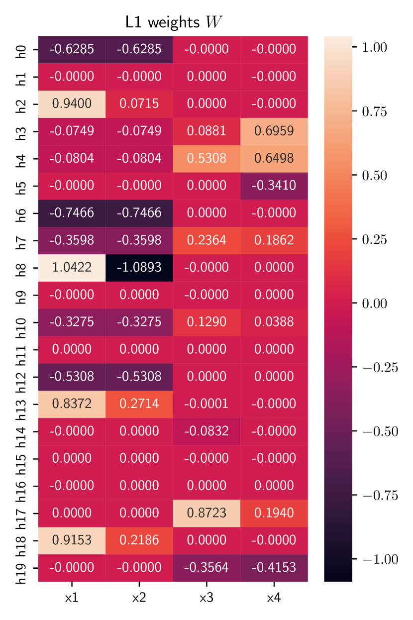
Figure 7: Concept relevance in terms of the weights $W$ of a standard linear layer (not entropy layer) used as the first layer of the network trained by minimizing the L1 loss (model A).

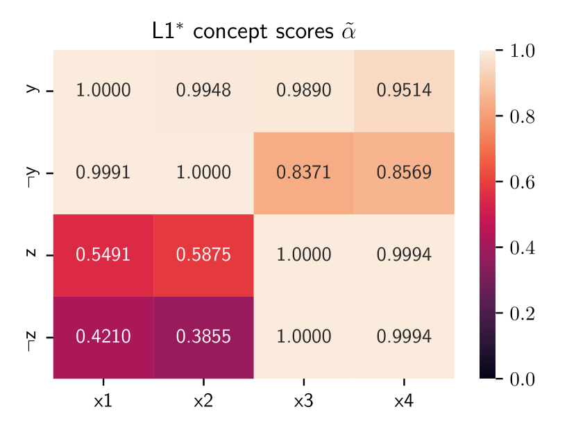
Figure 8: Concept scores $\tilde{\alpha}$ for the Entropy layer (first layer of the network) trained by minimizing the L1 loss instead of the entropy loss of Eq. 7 (model B).

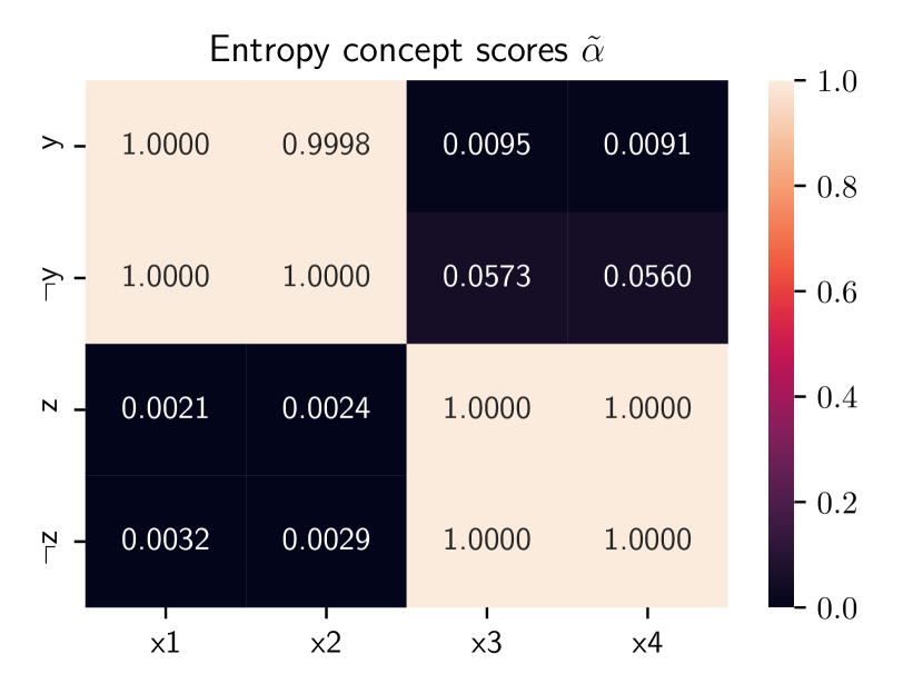
Figure 9: Concept scores $\tilde{\alpha}$ for the Entropy layer (first layer of the network) trained by minimizing the entropy loss in Eq. 7 (model C).

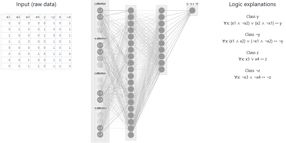
Figure 10: Visualization of the Entropy-based Network (model C) trained on the toy dataset after $18000$ epochs. The first layer of the network is the Entropy Layer. The gray-scale intensity of the input neurons represents the concept scores $\tilde{\alpha}$. The darker the input neuron, the higher the score ($\tilde{\alpha}_{i}^{j}\rightarrow 1$), the lighter the input neuron, the lower the score ($\tilde{\alpha}_{i}^{j}\rightarrow 0$).

A.6 Impact of hyperparameters on the logic explanations

We measured the impact of the hyperparameters on the quality of the explanations on the vDem dataset. Table 9 summarizes the average model accuracy, explanation accuracy, and explanation complexity obtained by running a 5-fold cross validation on the grid where $\lambda\in[10^{-3},10^{-6}]$ and $\tau\in[4,6]$ for the vDem dataset. The reported variance is the standard error of the mean. All the other parameters of the network (number of layers, number of epochs, etc…) have been set as reported in the main experimental section. Overall, the variation (within the defined grid) of the hyperparameters produced some minor effects on the quality of the explanations in terms of accuracy and complexity.

Table 9: Impact of the hyperparameters on the quality of the model and the explanations.

$(\tau,\lambda)$	Model accuracy	Explanation accuracy	Explanation complexity
$(4,10^{-6})$	$94.15\pm 0.53$	$89.68\pm 0.36$	$1.70\pm 0.20$
$(4,10^{-5})$	$94.56\pm 0.28$	$88.20\pm 1.05$	$2.50\pm 0.76$
$(4,10^{-4})$	$94.53\pm 0.42$	$87.73\pm 1.25$	$3.10\pm 0.83$
$(4,10^{-3})$	$94.62\pm 0.45$	$89.37\pm 0.73$	$2.00\pm 0.16$
$(5,10^{-6})$	$94.53\pm 0.65$	$89.91\pm 0.59$	$2.50\pm 0.50$
$(5,10^{-5})$	$94.86\pm 0.23$	$88.04\pm 1.29$	$1.60\pm 0.19$
$(5,10^{-4})$	$94.68\pm 0.48$	$88.20\pm 0.80$	$3.25\pm 0.92$
$(5,10^{-3})$	$94.53\pm 0.58$	$89.92\pm 0.39$	$2.00\pm 0.22$
$(6,10^{-6})$	$94.83\pm 0.49$	$85.53\pm 1.98$	$3.30\pm 0.64$
$(6,10^{-5})$	$94.56\pm 0.51$	$87.90\pm 0.98$	$2.70\pm 0.58$
$(6,10^{-4})$	$94.48\pm 0.73$	$87.22\pm 1.80$	$1.80\pm 0.25$
$(6,10^{-3})$	$94.05\pm 0.58$	$90.15\pm 0.68$	$2.12\pm 0.43$

A.7 Logic formulas

Table 10 reports a selection of the rule extracted by each method in all the experiments presented in the main paper. For all methods we report only the explanations of the first class for the first split of the Cross-validation. At last, for the Entropy-based method only, Tables 11, 12, 13, LABEL:tab:cub_rules resume the explanations of all classes in all experiments. For simplicity, in the following tables we dropped the universal quantifier for all formulas.

Table 10: Comparison of the formulas obtained in the first run of each experiment for all methods. We dropped the arguments in the logic predicates as well as the universal quantifiers for simplicity. Only the formula explaining the first class has been reported. Ellipses are used to truncate overly long formulas.

Dataset	Method	Formulas
MIMIC-II	Entropy	recover $\leftrightarrow$ $\neg$liver_flg $\wedge$ $\neg$stroke_flg $\wedge$ $\neg$mal_flg
	DTree	recover $\leftrightarrow$ (age_high <0.5 $\wedge$ mal_flg <0.5 $\wedge$ stroke_flg <0.5 $\wedge$ age_normal <0.5 $\wedge$ iv_day_1_normal <0.5) $\vee$ (age_high <0.5 $\wedge$ mal_flg <0.5 $\wedge$ stroke_flg <0.5 $\wedge$ age_normal <0.5 $\wedge$ iv_day_1_normal >0.5) $\vee$ (age_high <0.5 $\wedge$ …
	BRL	recover $\leftrightarrow$ (age_low $\wedge$ sofa_first_low $\wedge$ $\neg$(mal_flg $\wedge$ $\neg$weight_first_normal)) $\vee$ (age_high $\wedge$ $\neg$service_num_normal $\wedge$ $\neg$(age_low $\wedge$ sofa_first_low) $\wedge$ $\neg$(chf_flg $\wedge$ $\neg$day_icu_intime_num_high) $\wedge$ $\neg$(mal_flg $\wedge$ $\neg$weight_first_normal) $\wedge$ $\neg$(stroke_flg $\wedge$ …
	$\psi$ Net	recover $\leftrightarrow$ (iv_day_1_normal $\wedge$ $\neg$age_high $\wedge$ $\neg$hour_icu_intime_normal $\wedge$ $\neg$sofa_first_normal) $\vee$ (mal_flg $\wedge$ $\neg$age_high $\wedge$ $\neg$hour_icu_intime_normal $\wedge$ $\neg$sofa_first_normal) $\vee$ …
V-Dem	Entropy	non_electoral_democracy $\leftrightarrow$ $\neg$v2xel_frefair $\vee$ $\neg$v2x_elecoff $\vee$ $\neg$v2x_cspart $\vee$ $\neg$v2xeg_eqaccess $\vee$ $\neg$v2xeg_eqdr
	DTree	non_electoral_democracy $\leftrightarrow$ (v2xel_frefair <0.5 $\wedge$ v2xdl_delib <0.5 $\wedge$ v2x_frassoc_thick <0.5) $\vee$ (v2xel_frefair <0.5 $\wedge$ v2xdl_delib <0.5 $\wedge$ v2x_frassoc_thick >0.5 $\wedge$ v2x_freexp_altinf <0.5 $\wedge$ v2xeg_eqprotec <0.5) $\vee$ …
	BRL	non_electoral_democracy $\leftrightarrow$ $\neg$v2x_cspart $\vee$ $\neg$v2x_elecoff $\vee$ $\neg$v2x_frassoc_thick $\vee$ $\neg$v2x_freexp_altinf $\vee$ $\neg$v2xcl_rol $\vee$ ($\neg$v2x_mpi $\wedge$ $\neg$v2xel_frefair)
	$\psi$ Net	non_electoral_democracy $\leftrightarrow$ $\neg$v2xeg_eqaccess $\vee$ (v2x_egal $\wedge$ $\neg$v2x_frassoc_thick) $\vee$ (v2xeg_eqdr $\wedge$ $\neg$v2x_egal) $\vee$ (v2xel_frefair $\wedge$ $\neg$v2x_frassoc_thick) $\vee$ ($\neg$v2x_cspart $\wedge$ $\neg$v2x_suffr) $\vee$ ($\neg$v2x_frassoc_thick $\wedge$ $\neg$v2x_suffr) $\vee$ …
MNIST	Entropy	even $\leftrightarrow$ (zero $\wedge$ $\neg$one $\wedge$ $\neg$two $\wedge$ $\neg$three $\wedge$ $\neg$four $\wedge$ $\neg$five $\wedge$ $\neg$six $\wedge$ $\neg$seven $\wedge$ $\neg$eight $\wedge$ $\neg$nine) $\vee$ (two $\wedge$ $\neg$zero $\wedge$ $\neg$one $\wedge$ $\neg$three $\wedge$ $\neg$four $\wedge$ $\neg$five $\wedge$ $\neg$six $\wedge$ $\neg$seven $\wedge$ $\neg$eight $\wedge$ $\neg$nine) $\vee$ (four $\wedge$ $\neg$zero $\wedge$ …
	DTree	even $\leftrightarrow$ (one <0.54 $\wedge$ nine <1.97$\cdot 10^{-}5$ $\wedge$ three <0.00 $\wedge$ five <0.09 $\wedge$ seven <0.20) $\vee$ (one <0.54 $\wedge$ nine <1.97$\cdot 10^{-}5$ $\wedge$ three <0.00 $\wedge$ five >0.09 $\wedge$ two >0.97) $\vee$ (one <0.54 $\wedge$ nine <1.97$\cdot 10^{-}5$ $\wedge$ three >0.00 $\wedge$ two <0.99 $\wedge$ eight >1.00) $\vee$ …
	BRL	even $\leftrightarrow$ (two $\wedge$ $\neg$one $\wedge$ $\neg$seven $\wedge$ $\neg$three $\wedge$ $\neg$(seven $\wedge$ $\neg$two)) $\vee$ (four $\wedge$ $\neg$five $\wedge$ $\neg$nine $\wedge$ $\neg$seven $\wedge$ $\neg$three $\wedge$ $\neg$(seven $\wedge$ $\neg$two) $\wedge$ $\neg$(two $\wedge$ $\neg$one)) $\vee$ (four $\wedge$ $\neg$five $\wedge$ $\neg$seven $\wedge$ $\neg$three $\wedge$ $\neg$(four $\wedge$ $\neg$nine) $\wedge$ $\neg$(seven $\wedge$ …
	$\psi$ Net	even $\leftrightarrow$ (four $\wedge$ nine $\wedge$ six $\wedge$ three $\wedge$ zero $\wedge$ $\neg$eight $\wedge$ $\neg$one $\wedge$ $\neg$seven) $\vee$ (four $\wedge$ nine $\wedge$ six $\wedge$ two $\wedge$ zero $\wedge$ $\neg$eight $\wedge$ $\neg$one $\wedge$ $\neg$seven) $\vee$ (eight $\wedge$ six $\wedge$ $\neg$four $\wedge$ $\neg$nine $\wedge$ $\neg$seven $\wedge$ $\neg$three $\wedge$ $\neg$two) $\vee$ (eight $\wedge$ six $\wedge$…
CUB	Entropy	black_footed_albatross $\leftrightarrow$ has_bill_length_about_the_same_as_head $\wedge$ has_wing_pattern_solid $\wedge$ $\neg$has_upper_tail_color_grey $\wedge$ $\neg$has_belly_color_white $\wedge$ $\neg$has_wing_shape_roundedwings $\wedge$ $\neg$has_bill_color_black
	DTree	black_footed_albatross $\leftrightarrow$ (has_back_pattern_striped <0.46 $\wedge$ has_back_color_buff <0.69 $\wedge$ has_upper_tail_color_white <0.59 $\wedge$ has_under_tail_color_buff <0.82 $\wedge$ has_shape_perchinglike <0.66 $\wedge$ …
	BRL	black_footed_albatross $\leftrightarrow$ (has_back_pattern_striped $\wedge$ has_belly_color_black $\wedge$ has_bill_shape_hooked_seabird $\wedge$ $\neg$has_belly_color_white) $\vee$ (has_back_pattern_striped $\wedge$ …
	$\psi$ Net	black_footed_albatross $\leftrightarrow$ (has_bill_shape_hooked_seabird $\wedge$ $\neg$has_breast_color_white $\wedge$ $\neg$has_size_small_5__9_in $\wedge$ $\neg$has_wing_color_grey) $\vee$ (has_bill_shape_hooked_seabird $\wedge$ …

Table 11: Formulas extracted from the MIMIC-II dataset.

Formulas

recover $\leftrightarrow$ $\neg$liver_flg $\wedge$ $\neg$stroke_flg $\wedge$ $\neg$mal_flg

non_recover $\leftrightarrow$ mal_flg $\vee$ (age_HIGH $\wedge$ $\neg$iv_day_1_NORMAL)

Table 12: Formulas extracted from the V-Dem dataset.

Formulas

non_electoral_democracy $\leftrightarrow$ $\neg$v2xel_frefair $\vee$ $\neg$v2x_elecoff $\vee$ $\neg$v2x_cspart $\vee$ $\neg$v2xeg_eqaccess $\vee$ $\neg$v2xeg_eqdr

electoral_democracy $\leftrightarrow$ v2xel_frefair $\wedge$ v2x_elecoff $\wedge$ v2x_cspart

Table 13: Formulas extracted from the MNIST dataset.

Formulas

even $\leftrightarrow$ (zero $\wedge$ $\neg$one $\wedge$ $\neg$two $\wedge$ $\neg$three $\wedge$ $\neg$four $\wedge$ $\neg$five $\wedge$ $\neg$six $\wedge$ $\neg$seven $\wedge$ $\neg$eight $\wedge$ $\neg$nine) $\vee$ (two $\wedge$ $\neg$zero $\wedge$ $\neg$one $\wedge$ $\neg$three $\wedge$ $\neg$four $\wedge$ $\neg$five $\wedge$ $\neg$six $\wedge$ $\neg$seven $\wedge$ $\neg$eight $\wedge$ $\neg$nine) $\vee$ (four $\wedge$ $\neg$zero $\wedge$ $\neg$one $\wedge$ $\neg$two $\wedge$ $\neg$three $\wedge$ $\neg$five $\wedge$ $\neg$six $\wedge$ $\neg$seven $\wedge$ $\neg$eight $\wedge$ $\neg$nine) $\vee$ (six $\wedge$ $\neg$zero $\wedge$ $\neg$one $\wedge$ $\neg$two $\wedge$ $\neg$three $\wedge$ $\neg$four $\wedge$ $\neg$five $\wedge$ $\neg$seven $\wedge$ $\neg$eight $\wedge$ $\neg$nine) $\vee$ (eight $\wedge$ $\neg$zero $\wedge$ $\neg$one $\wedge$ $\neg$two $\wedge$ $\neg$three $\wedge$ $\neg$four $\wedge$ $\neg$five $\wedge$ $\neg$six $\wedge$ $\neg$seven $\wedge$ $\neg$nine)

odd $\leftrightarrow$ (one $\wedge$ $\neg$zero $\wedge$ $\neg$two $\wedge$ $\neg$three $\wedge$ $\neg$four $\wedge$ $\neg$five $\wedge$ $\neg$six $\wedge$ $\neg$seven $\wedge$ $\neg$eight $\wedge$ $\neg$nine) $\vee$ (three $\wedge$ $\neg$zero $\wedge$ $\neg$one $\wedge$ $\neg$two $\wedge$ $\neg$four $\wedge$ $\neg$five $\wedge$ $\neg$six $\wedge$ $\neg$seven $\wedge$ $\neg$eight $\wedge$ $\neg$nine) $\vee$ (five $\wedge$ $\neg$zero $\wedge$ $\neg$one $\wedge$ $\neg$two $\wedge$ $\neg$three $\wedge$ $\neg$four $\wedge$ $\neg$six $\wedge$ $\neg$seven $\wedge$ $\neg$eight $\wedge$ $\neg$nine) $\vee$ (seven $\wedge$ $\neg$zero $\wedge$ $\neg$one $\wedge$ $\neg$two $\wedge$ $\neg$three $\wedge$ $\neg$four $\wedge$ $\neg$five $\wedge$ $\neg$six $\wedge$ $\neg$eight $\wedge$ $\neg$nine) $\vee$ (nine $\wedge$ $\neg$zero $\wedge$ $\neg$one $\wedge$ $\neg$two $\wedge$ $\neg$three $\wedge$ $\neg$four $\wedge$ $\neg$five $\wedge$ $\neg$six $\wedge$ $\neg$seven $\wedge$ $\neg$eight)

Table 14: Formulas extracted from the CUB dataset.

Formulas
Black_footed_Albatross $\leftrightarrow$ has_bill_length_about_the_same_as_head $\wedge$ has_wing_pattern_solid $\wedge$ $\neg$has_upper_tail_color_grey $\wedge$ $\neg$has_belly_color_white $\wedge$ $\neg$has_wing_shape_roundedwings $\wedge$ $\neg$has_bill_color_black
Laysan_Albatross $\leftrightarrow$ has_crown_color_white $\wedge$ has_wing_pattern_solid $\wedge$ $\neg$has_under_tail_color_white
Sooty_Albatross $\leftrightarrow$ has_upper_tail_color_grey $\wedge$ has_size_medium_9__16_in $\wedge$ has_bill_color_black $\wedge$ $\neg$has_belly_color_white
Groove_billed_Ani $\leftrightarrow$ has_breast_color_black $\wedge$ has_leg_color_black $\wedge$ $\neg$has_bill_shape_allpurpose $\wedge$ $\neg$has_bill_length_about_the_same_as_head $\wedge$ $\neg$has_wing_shape_roundedwings
Crested_Auklet $\leftrightarrow$ has_nape_color_black $\wedge$ $\neg$has_eye_color_black $\wedge$ $\neg$has_belly_color_white
Least_Auklet $\leftrightarrow$ has_breast_color_black $\wedge$ has_breast_color_white $\wedge$ $\neg$has_nape_color_white $\wedge$ $\neg$has_size_small_5__9_in
Parakeet_Auklet $\leftrightarrow$ has_size_medium_9__16_in $\wedge$ has_primary_color_white $\wedge$ has_leg_color_grey
Rhinoceros_Auklet $\leftrightarrow$ has_size_medium_9__16_in $\wedge$ has_leg_color_buff
Brewer_Blackbird $\leftrightarrow$ has_breast_color_black $\wedge$ has_wing_shape_roundedwings $\wedge$ $\neg$has_bill_length_about_the_same_as_head $\wedge$ $\neg$has_shape_perchinglike
Red_winged_Blackbird $\leftrightarrow$ has_belly_color_black $\wedge$ has_wing_pattern_multicolored $\wedge$ $\neg$has_wing_color_white
Rusty_Blackbird $\leftrightarrow$ has_back_color_brown $\wedge$ has_belly_color_black $\wedge$ $\neg$has_crown_color_brown
Yellow_headed_Blackbird $\leftrightarrow$ has_forehead_color_yellow $\wedge$ has_primary_color_black
Bobolink $\leftrightarrow$ has_belly_color_black $\wedge$ $\neg$has_upper_tail_color_grey $\wedge$ $\neg$has_upper_tail_color_black
Indigo_Bunting $\leftrightarrow$ has_forehead_color_blue $\wedge$ has_back_pattern_solid $\wedge$ has_wing_pattern_multicolored
Lazuli_Bunting $\leftrightarrow$ has_leg_color_black $\wedge$ has_bill_color_grey $\wedge$ $\neg$has_under_tail_color_white
Painted_Bunting $\leftrightarrow$ has_nape_color_blue $\wedge$ has_leg_color_grey $\wedge$ has_bill_color_grey
Cardinal $\leftrightarrow$ has_forehead_color_red $\wedge$ has_wing_shape_roundedwings $\wedge$ has_wing_pattern_multicolored $\wedge$ $\neg$has_nape_color_black
Spotted_Catbird $\leftrightarrow$ has_leg_color_grey $\wedge$ $\neg$has_breast_pattern_solid $\wedge$ $\neg$has_breast_color_black $\wedge$ $\neg$has_belly_color_white $\wedge$ $\neg$has_crown_color_black
Gray_Catbird $\leftrightarrow$ has_under_tail_color_grey $\wedge$ has_belly_color_grey $\wedge$ has_crown_color_black $\wedge$ $\neg$has_primary_color_black
Yellow_breasted_Chat $\leftrightarrow$ has_primary_color_yellow $\wedge$ has_bill_color_black $\wedge$ $\neg$has_back_color_grey $\wedge$ $\neg$has_throat_color_grey $\wedge$ $\neg$has_throat_color_black $\wedge$ $\neg$has_nape_color_yellow $\wedge$ $\neg$has_belly_color_white
Eastern_Towhee $\leftrightarrow$ has_breast_color_black $\wedge$ has_nape_color_black $\wedge$ $\neg$has_belly_color_black $\wedge$ $\neg$has_tail_pattern_multicolored $\wedge$ $\neg$has_primary_color_white
Chuck_will_Widow $\leftrightarrow$ has_under_tail_color_brown $\wedge$ has_belly_color_buff $\wedge$ has_crown_color_brown $\wedge$ $\neg$has_bill_shape_allpurpose
Brandt_Cormorant $\leftrightarrow$ has_bill_shape_hooked_seabird $\wedge$ has_breast_color_black $\wedge$ $\neg$has_wing_shape_roundedwings
Red_faced_Cormorant $\leftrightarrow$ has_belly_color_black $\wedge$ $\neg$has_size_small_5__9_in $\wedge$ $\neg$has_bill_color_black
Pelagic_Cormorant $\leftrightarrow$ has_size_medium_9__16_in $\wedge$ has_leg_color_black $\wedge$ $\neg$has_bill_shape_hooked_seabird $\wedge$ $\neg$has_tail_shape_notched_tail $\wedge$ $\neg$has_belly_color_white $\wedge$ $\neg$has_wing_shape_roundedwings
Bronzed_Cowbird $\leftrightarrow$ has_belly_color_black $\wedge$ has_shape_perchinglike $\wedge$ has_wing_pattern_solid $\wedge$ $\neg$has_bill_shape_allpurpose $\wedge$ $\neg$has_underparts_color_yellow $\wedge$ $\neg$has_bill_length_about_the_same_as_head
Shiny_Cowbird $\leftrightarrow$ has_belly_color_black $\wedge$ has_shape_perchinglike $\wedge$ has_wing_pattern_solid $\wedge$ $\neg$has_wing_shape_roundedwings
Brown_Creeper $\leftrightarrow$ has_nape_color_buff $\wedge$ $\neg$has_shape_perchinglike
American_Crow $\leftrightarrow$ has_belly_color_black $\wedge$ has_shape_perchinglike $\wedge$ $\neg$has_breast_color_buff $\wedge$ $\neg$has_bill_length_shorter_than_head
Fish_Crow $\leftrightarrow$ has_bill_shape_allpurpose $\wedge$ has_bill_length_about_the_same_as_head $\wedge$ $\neg$has_under_tail_color_grey $\wedge$ $\neg$has_belly_color_white $\wedge$ $\neg$has_shape_perchinglike
Black_billed_Cuckoo $\leftrightarrow$ has_leg_color_grey $\wedge$ has_crown_color_brown
Mangrove_Cuckoo $\leftrightarrow$ has_belly_color_buff $\wedge$ has_leg_color_grey $\wedge$ $\neg$has_back_color_black
Yellow_billed_Cuckoo $\leftrightarrow$ has_shape_perchinglike $\wedge$ has_tail_pattern_solid $\wedge$ has_primary_color_white $\wedge$ $\neg$has_bill_color_black
Gray_crowned_Rosy_Finch $\leftrightarrow$ has_under_tail_color_black $\wedge$ has_crown_color_grey $\wedge$ has_wing_pattern_striped
Purple_Finch $\leftrightarrow$ has_forehead_color_red $\wedge$ $\neg$has_wing_shape_roundedwings $\wedge$ $\neg$has_belly_pattern_solid $\wedge$ $\neg$has_bill_color_black
Northern_Flicker $\leftrightarrow$ has_belly_color_black $\wedge$ has_leg_color_grey $\wedge$ $\neg$has_nape_color_black
Acadian_Flycatcher $\leftrightarrow$ has_breast_color_white $\wedge$ has_leg_color_black $\wedge$ $\neg$has_under_tail_color_white $\wedge$ $\neg$has_bill_color_black
Great_Crested_Flycatcher $\leftrightarrow$ has_tail_pattern_solid $\wedge$ has_primary_color_grey $\wedge$ has_wing_pattern_striped
Least_Flycatcher $\leftrightarrow$ has_tail_shape_notched_tail $\wedge$ has_tail_pattern_solid $\wedge$ $\neg$has_bill_shape_cone $\wedge$ $\neg$has_underparts_color_black $\wedge$ $\neg$has_back_color_brown $\wedge$ $\neg$has_breast_color_yellow $\wedge$ $\neg$has_throat_color_black $\wedge$ $\neg$has_bill_length_about_the_same_as_head $\wedge$ $\neg$has_primary_color_buff $\wedge$ $\neg$has_leg_color_black
Olive_sided_Flycatcher $\leftrightarrow$ has_belly_color_grey $\wedge$ has_belly_color_white
Scissor_tailed_Flycatcher $\leftrightarrow$ has_forehead_color_white $\wedge$ $\neg$has_under_tail_color_white $\wedge$ $\neg$has_shape_perchinglike $\wedge$ $\neg$has_tail_pattern_solid
Vermilion_Flycatcher $\leftrightarrow$ has_upper_tail_color_black $\wedge$ has_wing_shape_roundedwings $\wedge$ has_leg_color_black $\wedge$ $\neg$has_belly_color_white $\wedge$ $\neg$has_back_pattern_striped $\wedge$ $\neg$has_primary_color_black
Yellow_bellied_Flycatcher $\leftrightarrow$ has_tail_shape_notched_tail $\wedge$ has_wing_pattern_multicolored $\wedge$ $\neg$has_wing_shape_roundedwings $\wedge$ $\neg$has_primary_color_yellow $\wedge$ $\neg$has_bill_color_black
Frigatebird $\leftrightarrow$ has_underparts_color_black $\wedge$ has_underparts_color_white $\wedge$ has_head_pattern_plain $\wedge$ $\neg$has_shape_perchinglike
Northern_Fulmar $\leftrightarrow$ has_under_tail_color_white $\wedge$ has_crown_color_white $\wedge$ $\neg$has_upper_tail_color_white
Gadwall $\leftrightarrow$ has_under_tail_color_black $\wedge$ has_size_medium_9__16_in $\wedge$ has_bill_color_black $\wedge$ $\neg$has_leg_color_grey $\wedge$ $\neg$has_crown_color_black
American_Goldfinch $\leftrightarrow$ has_under_tail_color_black $\wedge$ has_back_pattern_solid $\wedge$ has_wing_pattern_multicolored $\wedge$ $\neg$has_belly_color_white $\wedge$ $\neg$has_bill_color_black
European_Goldfinch $\leftrightarrow$ has_leg_color_buff $\wedge$ has_wing_pattern_multicolored $\wedge$ $\neg$has_tail_pattern_solid
Boat_tailed_Grackle $\leftrightarrow$ has_throat_color_black $\wedge$ has_wing_shape_roundedwings $\wedge$ $\neg$has_bill_length_shorter_than_head $\wedge$ $\neg$has_size_small_5__9_in $\wedge$ $\neg$has_size_medium_9__16_in
Eared_Grebe $\leftrightarrow$ has_belly_color_grey $\wedge$ has_primary_color_black $\wedge$ $\neg$has_tail_pattern_solid
Horned_Grebe $\leftrightarrow$ has_primary_color_black $\wedge$ has_bill_color_black $\wedge$ $\neg$has_nape_color_black $\wedge$ $\neg$has_size_small_5__9_in $\wedge$ $\neg$has_belly_pattern_solid
Pied_billed_Grebe $\leftrightarrow$ has_under_tail_color_brown $\wedge$ has_size_medium_9__16_in
Western_Grebe $\leftrightarrow$ has_size_medium_9__16_in $\wedge$ has_primary_color_white $\wedge$ $\neg$has_throat_color_black $\wedge$ $\neg$has_under_tail_color_white
Blue_Grosbeak $\leftrightarrow$ has_under_tail_color_black $\wedge$ has_bill_color_grey $\wedge$ $\neg$has_tail_pattern_solid $\wedge$ $\neg$has_crown_color_black
Evening_Grosbeak $\leftrightarrow$ has_nape_color_brown $\wedge$ has_tail_pattern_solid $\wedge$ $\neg$has_nape_color_buff $\wedge$ $\neg$has_back_pattern_solid
Pine_Grosbeak $\leftrightarrow$ has_under_tail_color_grey $\wedge$ has_leg_color_black $\wedge$ has_wing_pattern_multicolored $\wedge$ $\neg$has_back_pattern_solid
Rose_breasted_Grosbeak $\leftrightarrow$ has_bill_shape_cone $\wedge$ has_wing_shape_roundedwings $\wedge$ has_primary_color_white $\wedge$ $\neg$has_nape_color_buff
Pigeon_Guillemot $\leftrightarrow$ has_underparts_color_black $\wedge$ has_size_medium_9__16_in $\wedge$ $\neg$has_leg_color_black
California_Gull $\leftrightarrow$ has_under_tail_color_black $\wedge$ has_wing_pattern_solid $\wedge$ $\neg$has_back_pattern_solid
Glaucous_winged_Gull $\leftrightarrow$ has_upper_tail_color_white $\wedge$ has_under_tail_color_grey
Heermann_Gull $\leftrightarrow$ has_nape_color_grey $\wedge$ has_crown_color_white $\wedge$ $\neg$has_shape_perchinglike
Herring_Gull $\leftrightarrow$ has_size_medium_9__16_in $\wedge$ has_primary_color_grey $\wedge$ has_wing_pattern_solid $\wedge$ $\neg$has_upper_tail_color_grey $\wedge$ $\neg$has_upper_tail_color_black
Ivory_Gull $\leftrightarrow$ has_leg_color_black $\wedge$ has_bill_color_grey $\wedge$ $\neg$has_shape_perchinglike
Ring_billed_Gull $\leftrightarrow$ has_under_tail_color_white $\wedge$ has_bill_color_black $\wedge$ $\neg$has_head_pattern_plain $\wedge$ $\neg$has_forehead_color_black $\wedge$ $\neg$has_shape_perchinglike $\wedge$ $\neg$has_wing_pattern_striped
Slaty_backed_Gull $\leftrightarrow$ has_upperparts_color_black $\wedge$ has_forehead_color_white $\wedge$ has_size_medium_9__16_in $\wedge$ $\neg$has_upper_tail_color_grey
Western_Gull $\leftrightarrow$ has_crown_color_white $\wedge$ $\neg$has_shape_perchinglike $\wedge$ $\neg$has_back_pattern_solid
Anna_Hummingbird $\leftrightarrow$ has_size_very_small_3__5_in $\wedge$ $\neg$has_breast_color_white $\wedge$ $\neg$has_wing_shape_roundedwings
Ruby_throated_Hummingbird $\leftrightarrow$ has_belly_color_white $\wedge$ has_leg_color_black $\wedge$ $\neg$has_wing_shape_roundedwings $\wedge$ $\neg$has_size_small_5__9_in $\wedge$ $\neg$has_back_pattern_solid
Rufous_Hummingbird $\leftrightarrow$ has_size_very_small_3__5_in $\wedge$ has_wing_pattern_multicolored $\wedge$ $\neg$has_shape_perchinglike
Green_Violetear $\leftrightarrow$ has_nape_color_blue $\wedge$ $\neg$has_bill_length_shorter_than_head
Long_tailed_Jaeger $\leftrightarrow$ (has_wing_color_grey $\wedge$ has_under_tail_color_black $\wedge$ $\neg$has_back_color_grey $\wedge$ $\neg$has_bill_length_shorter_than_head) $\vee$ (has_under_tail_color_black $\wedge$ $\neg$has_wing_color_black $\wedge$ $\neg$has_back_color_grey $\wedge$ $\neg$has_size_small_5__9_in $\wedge$ $\neg$has_primary_color_brown)
Pomarine_Jaeger $\leftrightarrow$ has_size_medium_9__16_in $\wedge$ has_leg_color_black $\wedge$ has_crown_color_black $\wedge$ $\neg$has_breast_color_black $\wedge$ $\neg$has_under_tail_color_white
Blue_Jay $\leftrightarrow$ has_forehead_color_blue $\wedge$ has_under_tail_color_black $\wedge$ has_leg_color_black
Florida_Jay $\leftrightarrow$ has_breast_pattern_multicolored $\wedge$ has_back_pattern_multicolored
Green_Jay $\leftrightarrow$ has_under_tail_color_yellow $\wedge$ has_leg_color_grey $\wedge$ $\neg$has_nape_color_grey $\wedge$ $\neg$has_crown_color_black
Dark_eyed_Junco $\leftrightarrow$ has_underparts_color_white $\wedge$ has_throat_color_grey
Tropical_Kingbird $\leftrightarrow$ has_forehead_color_grey $\wedge$ has_primary_color_yellow $\wedge$ has_bill_color_black $\wedge$ $\neg$has_back_pattern_multicolored
Gray_Kingbird $\leftrightarrow$ has_forehead_color_grey $\wedge$ $\neg$has_bill_length_shorter_than_head $\wedge$ $\neg$has_under_tail_color_black
Belted_Kingfisher $\leftrightarrow$ has_breast_pattern_multicolored $\wedge$ has_wing_shape_roundedwings $\wedge$ $\neg$has_back_color_black $\wedge$ $\neg$has_bill_length_shorter_than_head
Green_Kingfisher $\leftrightarrow$ has_throat_color_white $\wedge$ has_tail_pattern_solid $\wedge$ $\neg$has_breast_color_white $\wedge$ $\neg$has_belly_pattern_solid
Pied_Kingfisher $\leftrightarrow$ has_breast_color_black $\wedge$ has_wing_shape_roundedwings $\wedge$ has_leg_color_black $\wedge$ $\neg$has_wing_pattern_solid $\wedge$ $\neg$has_wing_pattern_striped $\wedge$ $\neg$has_wing_pattern_multicolored
Ringed_Kingfisher $\leftrightarrow$ has_size_small_5__9_in $\wedge$ has_primary_color_grey $\wedge$ $\neg$has_nape_color_grey $\wedge$ $\neg$has_wing_shape_roundedwings $\wedge$ $\neg$has_wing_pattern_multicolored
White_breasted_Kingfisher $\leftrightarrow$ has_crown_color_brown $\wedge$ has_wing_pattern_multicolored
Red_legged_Kittiwake $\leftrightarrow$ has_wing_color_white $\wedge$ has_bill_length_shorter_than_head $\wedge$ $\neg$has_tail_shape_notched_tail $\wedge$ $\neg$has_forehead_color_blue $\wedge$ $\neg$has_forehead_color_grey $\wedge$ $\neg$has_nape_color_brown $\wedge$ $\neg$has_back_pattern_striped $\wedge$ $\neg$has_tail_pattern_multicolored $\wedge$ $\neg$has_crown_color_black
Horned_Lark $\leftrightarrow$ has_primary_color_buff $\wedge$ $\neg$has_under_tail_color_black $\wedge$ $\neg$has_wing_shape_roundedwings $\wedge$ $\neg$has_back_pattern_solid $\wedge$ $\neg$has_wing_pattern_striped
Pacific_Loon $\leftrightarrow$ has_size_medium_9__16_in $\wedge$ has_leg_color_grey $\wedge$ $\neg$has_belly_pattern_solid
Mallard $\leftrightarrow$ has_breast_color_brown $\wedge$ has_wing_pattern_multicolored $\wedge$ $\neg$has_forehead_color_yellow
Western_Meadowlark $\leftrightarrow$ has_belly_color_yellow $\wedge$ has_leg_color_buff $\wedge$ has_bill_color_grey
Hooded_Merganser $\leftrightarrow$ has_tail_pattern_solid $\wedge$ has_bill_color_black $\wedge$ $\neg$has_eye_color_black
Red_breasted_Merganser $\leftrightarrow$ has_forehead_color_black $\wedge$ $\neg$has_belly_color_white $\wedge$ $\neg$has_belly_pattern_solid $\wedge$ $\neg$has_wing_pattern_striped
Mockingbird $\leftrightarrow$ has_forehead_color_grey $\wedge$ has_wing_shape_roundedwings $\wedge$ $\neg$has_upperparts_color_grey
Nighthawk $\leftrightarrow$ has_breast_color_brown $\wedge$ $\neg$has_underparts_color_brown $\wedge$ $\neg$has_belly_pattern_solid
Clark_Nutcracker $\leftrightarrow$ has_forehead_color_grey $\wedge$ has_leg_color_grey $\wedge$ has_wing_pattern_multicolored $\wedge$ $\neg$has_primary_color_yellow
White_breasted_Nuthatch $\leftrightarrow$ has_back_pattern_multicolored $\wedge$ has_tail_pattern_multicolored $\wedge$ $\neg$has_nape_color_white $\wedge$ $\neg$has_belly_color_yellow
Baltimore_Oriole $\leftrightarrow$ has_breast_color_yellow $\wedge$ has_under_tail_color_yellow $\wedge$ $\neg$has_wing_shape_roundedwings
Hooded_Oriole $\leftrightarrow$ has_breast_color_yellow $\wedge$ has_back_pattern_solid $\wedge$ has_tail_pattern_solid $\wedge$ has_wing_pattern_multicolored
Orchard_Oriole $\leftrightarrow$ has_leg_color_grey $\wedge$ has_crown_color_black $\wedge$ has_wing_pattern_multicolored $\wedge$ $\neg$has_under_tail_color_yellow $\wedge$ $\neg$has_belly_color_white
Scott_Oriole $\leftrightarrow$ has_under_tail_color_yellow $\wedge$ has_wing_pattern_multicolored $\wedge$ $\neg$has_back_pattern_solid $\wedge$ $\neg$has_back_pattern_multicolored
Ovenbird $\leftrightarrow$ has_breast_color_black $\wedge$ has_throat_color_white $\wedge$ has_wing_pattern_solid $\wedge$ $\neg$has_leg_color_grey
Brown_Pelican $\leftrightarrow$ has_wing_pattern_solid $\wedge$ $\neg$has_breast_pattern_solid $\wedge$ $\neg$has_back_pattern_solid $\wedge$ $\neg$has_primary_color_yellow
White_Pelican $\leftrightarrow$ has_crown_color_white $\wedge$ $\neg$has_head_pattern_plain $\wedge$ $\neg$has_under_tail_color_black $\wedge$ $\neg$has_size_medium_9__16_in $\wedge$ $\neg$has_shape_perchinglike
Western_Wood_Pewee $\leftrightarrow$ has_tail_pattern_solid $\wedge$ has_bill_color_black $\wedge$ has_crown_color_grey $\wedge$ $\neg$has_under_tail_color_grey $\wedge$ $\neg$has_wing_shape_roundedwings
Sayornis $\leftrightarrow$ has_upper_tail_color_brown $\wedge$ has_head_pattern_plain
American_Pipit $\leftrightarrow$ has_nape_color_buff $\wedge$ has_wing_shape_roundedwings $\wedge$ $\neg$has_belly_pattern_solid $\wedge$ $\neg$has_primary_color_brown
Whip_poor_Will $\leftrightarrow$ has_wing_shape_roundedwings $\wedge$ $\neg$has_belly_color_white $\wedge$ $\neg$has_shape_perchinglike $\wedge$ $\neg$has_leg_color_black $\wedge$ $\neg$has_crown_color_brown $\wedge$ $\neg$has_wing_pattern_solid
Horned_Puffin $\leftrightarrow$ has_throat_color_black $\wedge$ has_eye_color_black $\wedge$ $\neg$has_breast_color_black $\wedge$ $\neg$has_wing_shape_roundedwings $\wedge$ $\neg$has_shape_perchinglike
Common_Raven $\leftrightarrow$ has_wing_shape_roundedwings $\wedge$ has_size_medium_9__16_in $\wedge$ $\neg$has_bill_shape_hooked_seabird $\wedge$ $\neg$has_shape_perchinglike
White_necked_Raven $\leftrightarrow$ has_nape_color_white $\wedge$ $\neg$has_throat_color_white $\wedge$ $\neg$has_size_small_5__9_in
American_Redstart $\leftrightarrow$ has_underparts_color_black $\wedge$ has_wing_pattern_multicolored $\wedge$ $\neg$has_belly_color_black $\wedge$ $\neg$has_leg_color_grey $\wedge$ $\neg$has_crown_color_grey
Geococcyx $\leftrightarrow$ has_nape_color_brown $\wedge$ has_leg_color_grey $\wedge$ $\neg$has_primary_color_white
Loggerhead_Shrike $\leftrightarrow$ has_nape_color_grey $\wedge$ has_tail_pattern_multicolored $\wedge$ $\neg$has_tail_shape_notched_tail $\wedge$ $\neg$has_breast_color_yellow $\wedge$ $\neg$has_bill_length_about_the_same_as_head
Great_Grey_Shrike $\leftrightarrow$ has_forehead_color_grey $\wedge$ has_wing_shape_roundedwings $\wedge$ has_wing_pattern_multicolored $\wedge$ $\neg$has_upperparts_color_white $\wedge$ $\neg$has_back_pattern_multicolored
Baird_Sparrow $\leftrightarrow$ has_back_color_brown $\wedge$ has_tail_shape_notched_tail $\wedge$ $\neg$has_wing_shape_roundedwings
Black_throated_Sparrow $\leftrightarrow$ has_forehead_color_grey $\wedge$ has_belly_color_white $\wedge$ $\neg$has_throat_color_white $\wedge$ $\neg$has_wing_pattern_multicolored
Brewer_Sparrow $\leftrightarrow$ has_wing_shape_roundedwings $\wedge$ has_back_pattern_striped $\wedge$ has_primary_color_buff $\wedge$ $\neg$has_under_tail_color_brown $\wedge$ $\neg$has_size_very_small_3__5_in $\wedge$ $\neg$has_primary_color_brown $\wedge$ $\neg$has_crown_color_black
Chipping_Sparrow $\leftrightarrow$ has_nape_color_grey $\wedge$ has_back_pattern_striped $\wedge$ $\neg$has_upper_tail_color_buff
Clay_colored_Sparrow $\leftrightarrow$ has_throat_color_white $\wedge$ has_forehead_color_brown $\wedge$ has_primary_color_buff $\wedge$ $\neg$has_nape_color_brown
House_Sparrow $\leftrightarrow$ has_back_pattern_striped $\wedge$ has_bill_color_black $\wedge$ $\neg$has_breast_color_yellow $\wedge$ $\neg$has_forehead_color_black $\wedge$ $\neg$has_leg_color_grey
Field_Sparrow $\leftrightarrow$ has_belly_color_buff $\wedge$ has_wing_pattern_striped $\wedge$ $\neg$has_leg_color_buff
Fox_Sparrow $\leftrightarrow$ has_breast_pattern_striped $\wedge$ $\neg$has_back_pattern_solid $\wedge$ $\neg$has_wing_pattern_striped
Grasshopper_Sparrow $\leftrightarrow$ has_under_tail_color_buff $\wedge$ has_belly_color_buff $\wedge$ has_leg_color_buff
Harris_Sparrow $\leftrightarrow$ has_nape_color_buff $\wedge$ has_primary_color_white
Henslow_Sparrow $\leftrightarrow$ has_breast_color_black $\wedge$ has_leg_color_buff $\wedge$ $\neg$has_primary_color_yellow
Le_Conte_Sparrow $\leftrightarrow$ has_wing_shape_roundedwings $\wedge$ has_back_pattern_striped $\wedge$ $\neg$has_back_color_brown $\wedge$ $\neg$has_bill_color_black
Lincoln_Sparrow $\leftrightarrow$ has_size_very_small_3__5_in $\wedge$ has_wing_pattern_striped $\wedge$ $\neg$has_belly_pattern_solid $\wedge$ $\neg$has_crown_color_white
Nelson_Sharp_tailed_Sparrow $\leftrightarrow$ has_back_pattern_striped $\wedge$ $\neg$has_nape_color_buff $\wedge$ $\neg$has_size_small_5__9_in $\wedge$ $\neg$has_crown_color_black
Savannah_Sparrow $\leftrightarrow$ has_back_pattern_striped $\wedge$ $\neg$has_back_color_buff $\wedge$ $\neg$has_under_tail_color_black $\wedge$ $\neg$has_belly_pattern_solid $\wedge$ $\neg$has_leg_color_black
Seaside_Sparrow $\leftrightarrow$ has_shape_perchinglike $\wedge$ has_tail_pattern_solid $\wedge$ $\neg$has_belly_pattern_solid $\wedge$ $\neg$has_bill_color_black $\wedge$ $\neg$has_wing_pattern_solid
Song_Sparrow $\leftrightarrow$ has_nape_color_buff $\wedge$ has_back_pattern_striped $\wedge$ $\neg$has_forehead_color_black $\wedge$ $\neg$has_primary_color_buff
Tree_Sparrow $\leftrightarrow$ has_tail_shape_notched_tail $\wedge$ has_belly_color_white $\wedge$ has_back_pattern_striped $\wedge$ $\neg$has_back_color_buff $\wedge$ $\neg$has_under_tail_color_brown
Vesper_Sparrow $\leftrightarrow$ has_breast_color_white $\wedge$ has_back_pattern_striped $\wedge$ has_leg_color_buff $\wedge$ $\neg$has_under_tail_color_buff
White_crowned_Sparrow $\leftrightarrow$ has_forehead_color_black $\wedge$ has_nape_color_grey $\wedge$ $\neg$has_leg_color_buff
White_throated_Sparrow $\leftrightarrow$ has_forehead_color_yellow $\wedge$ has_primary_color_brown
Cape_Glossy_Starling $\leftrightarrow$ has_nape_color_blue $\wedge$ has_wing_pattern_solid
Bank_Swallow $\leftrightarrow$ has_bill_shape_cone $\wedge$ has_breast_color_white $\wedge$ has_bill_color_black $\wedge$ $\neg$has_forehead_color_blue $\wedge$ $\neg$has_forehead_color_black $\wedge$ $\neg$has_wing_pattern_solid
Barn_Swallow $\leftrightarrow$ has_back_pattern_solid $\wedge$ has_primary_color_black $\wedge$ has_bill_color_black $\wedge$ $\neg$has_belly_color_black $\wedge$ $\neg$has_shape_perchinglike $\wedge$ $\neg$has_leg_color_black
Cliff_Swallow $\leftrightarrow$ has_belly_color_buff $\wedge$ has_tail_pattern_solid $\wedge$ $\neg$has_back_pattern_solid
Tree_Swallow $\leftrightarrow$ has_primary_color_white $\wedge$ has_bill_color_black $\wedge$ $\neg$has_upperparts_color_black $\wedge$ $\neg$has_size_medium_9__16_in $\wedge$ $\neg$has_primary_color_brown
Scarlet_Tanager $\leftrightarrow$ has_upperparts_color_black $\wedge$ has_forehead_color_red $\wedge$ $\neg$has_bill_length_about_the_same_as_head $\wedge$ $\neg$has_under_tail_color_white
Summer_Tanager $\leftrightarrow$ has_tail_shape_notched_tail $\wedge$ has_leg_color_grey $\wedge$ $\neg$has_throat_color_white $\wedge$ $\neg$has_forehead_color_black $\wedge$ $\neg$has_primary_color_grey
Artic_Tern $\leftrightarrow$ has_head_pattern_capped $\wedge$ has_nape_color_black $\wedge$ $\neg$has_bill_shape_dagger $\wedge$ $\neg$has_upper_tail_color_black
Black_Tern $\leftrightarrow$ has_belly_color_black $\wedge$ $\neg$has_under_tail_color_black $\wedge$ $\neg$has_wing_shape_roundedwings
Caspian_Tern $\leftrightarrow$ has_head_pattern_capped $\wedge$ has_size_medium_9__16_in $\wedge$ has_wing_pattern_solid $\wedge$ $\neg$has_nape_color_black
Common_Tern $\leftrightarrow$ has_wing_color_grey $\wedge$ has_back_color_white $\wedge$ $\neg$has_forehead_color_white
Elegant_Tern $\leftrightarrow$ has_forehead_color_white $\wedge$ has_size_medium_9__16_in $\wedge$ $\neg$has_head_pattern_plain
Forsters_Tern $\leftrightarrow$ has_head_pattern_capped $\wedge$ has_nape_color_black $\wedge$ has_bill_color_black $\wedge$ $\neg$has_upper_tail_color_black
Least_Tern $\leftrightarrow$ has_forehead_color_white $\wedge$ has_crown_color_black $\wedge$ has_wing_pattern_solid
Green_tailed_Towhee $\leftrightarrow$ has_wing_shape_roundedwings $\wedge$ has_bill_color_grey $\wedge$ $\neg$has_throat_color_yellow $\wedge$ $\neg$has_nape_color_blue $\wedge$ $\neg$has_nape_color_brown
Brown_Thrasher $\leftrightarrow$ has_nape_color_brown $\wedge$ $\neg$has_forehead_color_brown $\wedge$ $\neg$has_belly_color_yellow $\wedge$ $\neg$has_leg_color_grey $\wedge$ $\neg$has_wing_pattern_striped
Sage_Thrasher $\leftrightarrow$ has_wing_pattern_striped $\wedge$ $\neg$has_eye_color_black
Black_capped_Vireo $\leftrightarrow$ has_nape_color_black $\wedge$ has_size_very_small_3__5_in $\wedge$ has_leg_color_grey
Blue_headed_Vireo $\leftrightarrow$ has_primary_color_grey $\wedge$ has_leg_color_grey $\wedge$ has_wing_pattern_striped
Philadelphia_Vireo $\leftrightarrow$ has_nape_color_grey $\wedge$ has_size_very_small_3__5_in $\wedge$ has_bill_color_grey
Red_eyed_Vireo $\leftrightarrow$ has_upperparts_color_buff $\wedge$ has_forehead_color_grey
Warbling_Vireo $\leftrightarrow$ has_nape_color_grey $\wedge$ has_size_very_small_3__5_in $\wedge$ has_primary_color_buff $\wedge$ $\neg$has_under_tail_color_buff
White_eyed_Vireo $\leftrightarrow$ has_tail_shape_notched_tail $\wedge$ has_tail_pattern_multicolored $\wedge$ $\neg$has_upperparts_color_black
Yellow_throated_Vireo $\leftrightarrow$ has_nape_color_yellow $\wedge$ has_belly_color_white
Bay_breasted_Warbler $\leftrightarrow$ has_wing_shape_roundedwings $\wedge$ has_back_pattern_striped $\wedge$ has_leg_color_grey
Black_and_white_Warbler $\leftrightarrow$ has_size_very_small_3__5_in $\wedge$ has_wing_pattern_striped $\wedge$ $\neg$has_primary_color_buff
Black_throated_Blue_Warbler $\leftrightarrow$ has_primary_color_black $\wedge$ has_wing_pattern_multicolored $\wedge$ $\neg$has_breast_color_yellow $\wedge$ $\neg$has_under_tail_color_black
Blue_winged_Warbler $\leftrightarrow$ has_back_color_grey $\wedge$ $\neg$has_nape_color_grey $\wedge$ $\neg$has_back_pattern_striped $\wedge$ $\neg$has_primary_color_grey $\wedge$ $\neg$has_crown_color_black
Canada_Warbler $\leftrightarrow$ has_under_tail_color_grey $\wedge$ has_nape_color_grey $\wedge$ has_belly_color_yellow $\wedge$ $\neg$has_back_pattern_multicolored $\wedge$ $\neg$has_primary_color_grey
Cape_May_Warbler $\leftrightarrow$ has_back_pattern_striped $\wedge$ has_bill_color_black $\wedge$ $\neg$has_belly_color_white $\wedge$ $\neg$has_belly_pattern_solid
Cerulean_Warbler $\leftrightarrow$ has_nape_color_blue $\wedge$ has_size_very_small_3__5_in $\wedge$ has_shape_perchinglike
Chestnut_sided_Warbler $\leftrightarrow$ has_underparts_color_white $\wedge$ has_upper_tail_color_grey $\wedge$ $\neg$has_wing_color_white $\wedge$ $\neg$has_bill_length_about_the_same_as_head $\wedge$ $\neg$has_belly_color_grey $\wedge$ $\neg$has_back_pattern_solid $\wedge$ $\neg$has_primary_color_yellow
Golden_winged_Warbler $\leftrightarrow$ has_forehead_color_yellow $\wedge$ has_wing_pattern_multicolored $\wedge$ $\neg$has_primary_color_yellow
Hooded_Warbler $\leftrightarrow$ has_forehead_color_yellow $\wedge$ has_primary_color_yellow $\wedge$ has_leg_color_buff $\wedge$ has_crown_color_black
Kentucky_Warbler $\leftrightarrow$ has_size_small_5__9_in $\wedge$ has_primary_color_yellow $\wedge$ has_leg_color_buff $\wedge$ has_crown_color_black
Magnolia_Warbler $\leftrightarrow$ has_forehead_color_grey $\wedge$ has_primary_color_black
Mourning_Warbler $\leftrightarrow$ has_forehead_color_grey $\wedge$ has_leg_color_buff
Myrtle_Warbler $\leftrightarrow$ has_leg_color_black $\wedge$ has_wing_pattern_striped $\wedge$ $\neg$has_tail_pattern_solid
Nashville_Warbler $\leftrightarrow$ has_under_tail_color_yellow $\wedge$ has_back_pattern_multicolored $\wedge$ $\neg$has_crown_color_black
Orange_crowned_Warbler $\leftrightarrow$ has_bill_shape_allpurpose $\wedge$ has_tail_pattern_multicolored $\wedge$ $\neg$has_breast_color_yellow $\wedge$ $\neg$has_primary_color_white $\wedge$ $\neg$has_crown_color_grey $\wedge$ $\neg$has_crown_color_black
Palm_Warbler $\leftrightarrow$ has_primary_color_yellow $\wedge$ has_wing_pattern_striped $\wedge$ $\neg$has_belly_color_yellow
Pine_Warbler $\leftrightarrow$ has_forehead_color_yellow $\wedge$ has_under_tail_color_grey $\wedge$ has_bill_color_grey
Prairie_Warbler $\leftrightarrow$ has_size_very_small_3__5_in $\wedge$ has_crown_color_yellow
Prothonotary_Warbler $\leftrightarrow$ has_under_tail_color_black $\wedge$ has_tail_pattern_solid $\wedge$ has_leg_color_grey $\wedge$ $\neg$has_upperparts_color_black
Swainson_Warbler $\leftrightarrow$ has_tail_shape_notched_tail $\wedge$ has_bill_length_about_the_same_as_head $\wedge$ $\neg$has_nape_color_grey $\wedge$ $\neg$has_primary_color_black
Tennessee_Warbler $\leftrightarrow$ has_upper_tail_color_grey $\wedge$ has_primary_color_yellow $\wedge$ $\neg$has_breast_color_yellow
Wilson_Warbler $\leftrightarrow$ has_under_tail_color_yellow $\wedge$ has_crown_color_black $\wedge$ $\neg$has_leg_color_grey
Worm_eating_Warbler $\leftrightarrow$ has_crown_color_yellow $\wedge$ $\neg$has_primary_color_yellow $\wedge$ $\neg$has_bill_color_black
Yellow_Warbler $\leftrightarrow$ has_under_tail_color_yellow $\wedge$ has_wing_pattern_striped
Northern_Waterthrush $\leftrightarrow$ has_size_small_5__9_in $\wedge$ has_tail_pattern_solid $\wedge$ has_leg_color_buff $\wedge$ $\neg$has_breast_color_yellow $\wedge$ $\neg$has_primary_color_grey
Louisiana_Waterthrush $\leftrightarrow$ has_breast_pattern_striped $\wedge$ has_wing_pattern_solid $\wedge$ $\neg$has_nape_color_brown
Bohemian_Waxwing $\leftrightarrow$ has_upper_tail_color_grey $\wedge$ has_wing_pattern_multicolored $\wedge$ $\neg$has_under_tail_color_grey
Cedar_Waxwing $\leftrightarrow$ has_nape_color_buff $\wedge$ has_wing_pattern_multicolored
American_Three_toed_Woodpecker $\leftrightarrow$ has_under_tail_color_white $\wedge$ has_tail_pattern_solid $\wedge$ has_leg_color_grey
Pileated_Woodpecker $\leftrightarrow$ has_nape_color_white $\wedge$ has_leg_color_grey $\wedge$ $\neg$has_primary_color_white
Red_bellied_Woodpecker $\leftrightarrow$ has_forehead_color_red $\wedge$ has_wing_pattern_striped
Red_cockaded_Woodpecker $\leftrightarrow$ has_head_pattern_capped $\wedge$ has_belly_color_black
Red_headed_Woodpecker $\leftrightarrow$ has_forehead_color_red $\wedge$ has_back_pattern_solid $\wedge$ has_wing_pattern_multicolored
Downy_Woodpecker $\leftrightarrow$ has_under_tail_color_white $\wedge$ has_back_pattern_multicolored $\wedge$ $\neg$has_wing_pattern_multicolored
Bewick_Wren $\leftrightarrow$ has_under_tail_color_brown $\wedge$ has_under_tail_color_black
Cactus_Wren $\leftrightarrow$ has_nape_color_white $\wedge$ $\neg$has_belly_color_white $\wedge$ $\neg$has_back_pattern_solid
Carolina_Wren $\leftrightarrow$ has_breast_color_buff $\wedge$ has_bill_color_grey $\wedge$ $\neg$has_leg_color_grey
House_Wren $\leftrightarrow$ has_breast_color_buff $\wedge$ $\neg$has_forehead_color_black $\wedge$ $\neg$has_wing_shape_roundedwings $\wedge$ $\neg$has_leg_color_black $\wedge$ $\neg$has_wing_pattern_solid
Marsh_Wren $\leftrightarrow$ has_nape_color_buff $\wedge$ has_belly_color_white $\wedge$ has_belly_color_buff
Rock_Wren $\leftrightarrow$ has_under_tail_color_buff $\wedge$ has_size_very_small_3__5_in $\wedge$ $\neg$has_crown_color_brown
Winter_Wren $\leftrightarrow$ has_breast_pattern_solid $\wedge$ has_breast_color_buff $\wedge$ $\neg$has_belly_pattern_solid
Common_Yellowthroat $\leftrightarrow$ has_forehead_color_black $\wedge$ has_under_tail_color_yellow $\wedge$ $\neg$has_crown_color_black

References

- Ahmad, Eckert, and Teredesai (2018) Ahmad, M. A.; Eckert, C.; and Teredesai, A. 2018. Interpretable machine learning in healthcare. In Proceedings of the 2018 ACM international conference on bioinformatics, computational biology, and health informatics, 559–560.
- Alvarez-Melis and Jaakkola (2018) Alvarez-Melis, D.; and Jaakkola, T. S. 2018. Towards robust interpretability with self-explaining neural networks. arXiv preprint arXiv:1806.07538.
- Angelino et al. (2018) Angelino, E.; Larus-Stone, N.; Alabi, D.; Seltzer, M.; and Rudin, C. 2018. Learning Certifiably Optimal Rule Lists for Categorical Data. arXiv:1704.01701.
- Anonymous (2021) Anonymous. 2021. Anonymous.
- Arrieta et al. (2020) Arrieta, A. B.; Díaz-Rodríguez, N.; Del Ser, J.; Bennetot, A.; Tabik, S.; Barbado, A.; García, S.; Gil-López, S.; Molina, D.; Benjamins, R.; et al. 2020. Explainable Artificial Intelligence (XAI): Concepts, taxonomies, opportunities and challenges toward responsible AI. Information Fusion, 58: 82–115.
- Battaglia et al. (2018) Battaglia, P. W.; Hamrick, J. B.; Bapst, V.; Sanchez-Gonzalez, A.; Zambaldi, V.; Malinowski, M.; Tacchetti, A.; Raposo, D.; Santoro, A.; Faulkner, R.; et al. 2018. Relational inductive biases, deep learning, and graph networks. arXiv preprint arXiv:1806.01261.
- Breiman et al. (1984) Breiman, L.; Friedman, J.; Stone, C. J.; and Olshen, R. A. 1984. Classification and regression trees. CRC press.
- Caruana et al. (2015) Caruana, R.; Lou, Y.; Gehrke, J.; Koch, P.; Sturm, M.; and Elhadad, N. 2015. Intelligible models for healthcare: Predicting pneumonia risk and hospital 30-day readmission. In Proceedings of the 21th ACM SIGKDD international conference on knowledge discovery and data mining, 1721–1730.
- Chen, Bei, and Rudin (2020) Chen, Z.; Bei, Y.; and Rudin, C. 2020. Concept whitening for interpretable image recognition. Nature Machine Intelligence, 2(12): 772–782.
- Ciravegna et al. (2020a) Ciravegna, G.; Giannini, F.; Gori, M.; Maggini, M.; and Melacci, S. 2020a. Human-driven FOL explanations of deep learning. In Twenty-Ninth International Joint Conference on Artificial Intelligence and Seventeenth Pacific Rim International Conference on Artificial Intelligence IJCAI-PRICAI-20, 2234–2240. International Joint Conferences on Artificial Intelligence Organization.
- Ciravegna et al. (2020b) Ciravegna, G.; Giannini, F.; Melacci, S.; Maggini, M.; and Gori, M. 2020b. A Constraint-Based Approach to Learning and Explanation. In AAAI, 3658–3665.
- Cohen (1995) Cohen, W. W. 1995. Fast effective rule induction. In Machine learning proceedings 1995, 115–123. Elsevier.
- Coppedge et al. (2021) Coppedge, M.; Gerring, J.; Knutsen, C. H.; Lindberg, S. I.; Teorell, J.; Altman, D.; Bernhard, M.; Cornell, A.; Fish, M. S.; Gastaldi, L.; et al. 2021. V-Dem Codebook v11.
- Cowan (2001) Cowan, N. 2001. The magical number 4 in short-term memory: A reconsideration of mental storage capacity. Behavioral and brain sciences, 24(1): 87–114.
- Cranmer et al. (2019) Cranmer, M. D.; Xu, R.; Battaglia, P.; and Ho, S. 2019. Learning symbolic physics with graph networks. arXiv preprint arXiv:1909.05862.
- Das and Rad (2020) Das, A.; and Rad, P. 2020. Opportunities and challenges in explainable artificial intelligence (xai): A survey. arXiv preprint arXiv:2006.11371.
- Devlin et al. (2018) Devlin, J.; Chang, M.-W.; Lee, K.; and Toutanova, K. 2018. Bert: Pre-training of deep bidirectional transformers for language understanding. arXiv preprint arXiv:1810.04805.
- Doshi-Velez and Kim (2017) Doshi-Velez, F.; and Kim, B. 2017. Towards a rigorous science of interpretable machine learning. arXiv preprint arXiv:1702.08608.
- Doshi-Velez and Kim (2018) Doshi-Velez, F.; and Kim, B. 2018. Considerations for evaluation and generalization in interpretable machine learning. In Explainable and interpretable models in computer vision and machine learning, 3–17. Springer.
- Dosovitskiy et al. (2020) Dosovitskiy, A.; Beyer, L.; Kolesnikov, A.; Weissenborn, D.; Zhai, X.; Unterthiner, T.; Dehghani, M.; Minderer, M.; Heigold, G.; Gelly, S.; et al. 2020. An image is worth 16x16 words: Transformers for image recognition at scale. arXiv preprint arXiv:2010.11929.
- EUGDPR (2017) EUGDPR. 2017. GDPR. General data protection regulation.
- Ghorbani et al. (2019) Ghorbani, A.; Wexler, J.; Zou, J.; and Kim, B. 2019. Towards automatic concept-based explanations. arXiv preprint arXiv:1902.03129.
- Goddard (2017) Goddard, M. 2017. The EU General Data Protection Regulation (GDPR): European regulation that has a global impact. International Journal of Market Research, 59(6): 703–705.
- Goldberger et al. (2000) Goldberger, A. L.; Amaral, L. A.; Glass, L.; Hausdorff, J. M.; Ivanov, P. C.; Mark, R. G.; Mietus, J. E.; Moody, G. B.; Peng, C.-K.; and Stanley, H. E. 2000. PhysioBank, PhysioToolkit, and PhysioNet: components of a new research resource for complex physiologic signals. circulation, 101(23): e215–e220.
- Guidotti et al. (2018) Guidotti, R.; Monreale, A.; Ruggieri, S.; Pedreschi, D.; Turini, F.; and Giannotti, F. 2018. Local rule-based explanations of black box decision systems. arXiv preprint arXiv:1805.10820.
- Han, Pei, and Yin (2000) Han, J.; Pei, J.; and Yin, Y. 2000. Mining frequent patterns without candidate generation. ACM sigmod record, 29(2): 1–12.
- Hastie and Tibshirani (1987) Hastie, T.; and Tibshirani, R. 1987. Generalized additive models: some applications. Journal of the American Statistical Association, 82(398): 371–386.
- He et al. (2016) He, K.; Zhang, X.; Ren, S.; and Sun, J. 2016. Deep residual learning for image recognition. In Proceedings of the IEEE conference on computer vision and pattern recognition, 770–778.
- Holte (1993) Holte, R. C. 1993. Very simple classification rules perform well on most commonly used datasets. Machine learning, 11(1): 63–90.
- Kazhdan et al. (2020) Kazhdan, D.; Dimanov, B.; Jamnik, M.; Liò, P.; and Weller, A. 2020. Now You See Me (CME): Concept-based Model Extraction. arXiv preprint arXiv:2010.13233.
- Kim et al. (2018a) Kim, B.; Gilmer, J.; Wattenberg, M.; and Viégas, F. 2018a. Tcav: Relative concept importance testing with linear concept activation vectors.
- Kim et al. (2018b) Kim, B.; Wattenberg, M.; Gilmer, J.; Cai, C.; Wexler, J.; Viegas, F.; et al. 2018b. Interpretability beyond feature attribution: Quantitative testing with concept activation vectors (tcav). In International conference on machine learning, 2668–2677. PMLR.
- Kindermans et al. (2019) Kindermans, P.-J.; Hooker, S.; Adebayo, J.; Alber, M.; Schütt, K. T.; Dähne, S.; Erhan, D.; and Kim, B. 2019. The (un) reliability of saliency methods. In Explainable AI: Interpreting, Explaining and Visualizing Deep Learning, 267–280. Springer.
- Koh et al. (2020) Koh, P. W.; Nguyen, T.; Tang, Y. S.; Mussmann, S.; Pierson, E.; Kim, B.; and Liang, P. 2020. Concept bottleneck models. In International Conference on Machine Learning, 5338–5348. PMLR.
- Krzywinski and Altman (2013) Krzywinski, M.; and Altman, N. 2013. Error bars: the meaning of error bars is often misinterpreted, as is the statistical significance of their overlap. Nature methods, 10(10): 921–923.
- LeCun (1998) LeCun, Y. 1998. The MNIST database of handwritten digits. http://yann. lecun. com/exdb/mnist/.
- Letham et al. (2015) Letham, B.; Rudin, C.; McCormick, T. H.; Madigan, D.; et al. 2015. Interpretable classifiers using rules and bayesian analysis: Building a better stroke prediction model. Annals of Applied Statistics, 9(3): 1350–1371.
- Loshchilov and Hutter (2017) Loshchilov, I.; and Hutter, F. 2017. Decoupled weight decay regularization. arXiv preprint arXiv:1711.05101.
- Lou, Caruana, and Gehrke (2012) Lou, Y.; Caruana, R.; and Gehrke, J. 2012. Intelligible models for classification and regression. In Proceedings of the 18th ACM SIGKDD international conference on Knowledge discovery and data mining, 150–158.
- Lundberg and Lee (2017) Lundberg, S.; and Lee, S.-I. 2017. A unified approach to interpreting model predictions. arXiv preprint arXiv:1705.07874.
- Ma, Husain, and Bays (2014) Ma, W. J.; Husain, M.; and Bays, P. M. 2014. Changing concepts of working memory. Nature neuroscience, 17(3): 347.
- Marler and Arora (2004) Marler, R. T.; and Arora, J. S. 2004. Survey of multi-objective optimization methods for engineering. Structural and multidisciplinary optimization, 26(6): 369–395.
- McCluskey (1956) McCluskey, E. J. 1956. Minimization of Boolean functions. The Bell System Technical Journal, 35(6): 1417–1444.
- McColl (1878) McColl, H. 1878. The calculus of equivalent statements (third paper). Proceedings of the London Mathematical Society, 1(1): 16–28.
- McKelvey and Zavoina (1975) McKelvey, R. D.; and Zavoina, W. 1975. A statistical model for the analysis of ordinal level dependent variables. Journal of Mathematical Sociology, 4(1): 103–120.
- Mendelson (2009) Mendelson, E. 2009. Introduction to mathematical logic. CRC press.
- Miller (1956) Miller, G. A. 1956. The magical number seven, plus or minus two: Some limits on our capacity for processing information. Psychological review, 63: 81–97.
- Minsky and Papert (2017) Minsky, M.; and Papert, S. A. 2017. Perceptrons: An introduction to computational geometry. MIT press.
- Molnar (2020) Molnar, C. 2020. Interpretable machine learning. Lulu. com.
- Paszke et al. (2019) Paszke, A.; Gross, S.; Massa, F.; Lerer, A.; Bradbury, J.; Chanan, G.; Killeen, T.; Lin, Z.; Gimelshein, N.; Antiga, L.; et al. 2019. Pytorch: An imperative style, high-performance deep learning library. arXiv preprint arXiv:1912.01703.
- Pedregosa et al. (2011) Pedregosa, F.; Varoquaux, G.; Gramfort, A.; Michel, V.; Thirion, B.; Grisel, O.; Blondel, M.; Prettenhofer, P.; Weiss, R.; Dubourg, V.; et al. 2011. Scikit-learn: Machine learning in Python. the Journal of machine Learning research, 12: 2825–2830.
- Pemstein et al. (2018) Pemstein, D.; Marquardt, K. L.; Tzelgov, E.; Wang, Y.-t.; Krusell, J.; and Miri, F. 2018. The V-Dem measurement model: latent variable analysis for cross-national and cross-temporal expert-coded data. V-Dem Working Paper, 21.
- Quine (1952) Quine, W. V. 1952. The problem of simplifying truth functions. The American mathematical monthly, 59(8): 521–531.
- Quinlan (1986) Quinlan, J. R. 1986. Induction of decision trees. Machine learning, 1(1): 81–106.
- Quinlan (2014) Quinlan, J. R. 2014. C4. 5: programs for machine learning. Elsevier.
- Rathmanner and Hutter (2011) Rathmanner, S.; and Hutter, M. 2011. A philosophical treatise of universal induction. Entropy, 13(6): 1076–1136.
- Ribeiro, Singh, and Guestrin (2016a) Ribeiro, M. T.; Singh, S.; and Guestrin, C. 2016a. ” Why should i trust you?” Explaining the predictions of any classifier. In Proceedings of the 22nd ACM SIGKDD international conference on knowledge discovery and data mining, 1135–1144.
- Ribeiro, Singh, and Guestrin (2016b) Ribeiro, M. T.; Singh, S.; and Guestrin, C. 2016b. Model-agnostic interpretability of machine learning. arXiv preprint arXiv:1606.05386.
- Ribeiro, Singh, and Guestrin (2018) Ribeiro, M. T.; Singh, S.; and Guestrin, C. 2018. Anchors: High-precision model-agnostic explanations. In Proceedings of the AAAI Conference on Artificial Intelligence, volume 32.
- Rivest (1987) Rivest, R. L. 1987. Learning decision lists. Machine learning, 2(3): 229–246.
- Rudin et al. (2021) Rudin, C.; Chen, C.; Chen, Z.; Huang, H.; Semenova, L.; and Zhong, C. 2021. Interpretable machine learning: Fundamental principles and 10 grand challenges. arXiv preprint arXiv:2103.11251.
- Saeed et al. (2011) Saeed, M.; Villarroel, M.; Reisner, A. T.; Clifford, G.; Lehman, L.-W.; Moody, G.; Heldt, T.; Kyaw, T. H.; Moody, B.; and Mark, R. G. 2011. Multiparameter Intelligent Monitoring in Intensive Care II (MIMIC-II): a public-access intensive care unit database. Critical care medicine, 39(5): 952.
- Sato and Tsukimoto (2001) Sato, M.; and Tsukimoto, H. 2001. Rule extraction from neural networks via decision tree induction. In IJCNN’01. International Joint Conference on Neural Networks. Proceedings (Cat. No. 01CH37222), volume 3, 1870–1875. IEEE.
- Schmidt and Lipson (2009) Schmidt, M.; and Lipson, H. 2009. Distilling free-form natural laws from experimental data. science, 324(5923): 81–85.
- Selvaraju et al. (2017) Selvaraju, R. R.; Cogswell, M.; Das, A.; Vedantam, R.; Parikh, D.; and Batra, D. 2017. Grad-cam: Visual explanations from deep networks via gradient-based localization. In Proceedings of the IEEE international conference on computer vision, 618–626.
- Simon (1956) Simon, H. A. 1956. Rational choice and the structure of the environment. Psychological review, 63(2): 129.
- Simon (1957) Simon, H. A. 1957. Models of man; social and rational. New York: John Wiley and Sons, Inc.
- Simon (1979) Simon, H. A. 1979. Rational decision making in business organizations. The American economic review, 69(4): 493–513.
- Simonyan, Vedaldi, and Zisserman (2013) Simonyan, K.; Vedaldi, A.; and Zisserman, A. 2013. Deep inside convolutional networks: Visualising image classification models and saliency maps. arXiv preprint arXiv:1312.6034.
- Soklakov (2002) Soklakov, A. N. 2002. Occam’s razor as a formal basis for a physical theory. Foundations of Physics Letters, 15(2): 107–135.
- Su, Vargas, and Sakurai (2019) Su, J.; Vargas, D. V.; and Sakurai, K. 2019. One pixel attack for fooling deep neural networks. IEEE Transactions on Evolutionary Computation, 23(5): 828–841.
- Tavares et al. (2020) Tavares, A. R.; Avelar, P.; Flach, J. M.; Nicolau, M.; Lamb, L. C.; and Vardi, M. 2020. Understanding boolean function learnability on deep neural networks. arXiv preprint arXiv:2009.05908.
- Wah et al. (2011) Wah, C.; Branson, S.; Welinder, P.; Perona, P.; and Belongie, S. 2011. The Caltech-UCSD Birds-200-2011 Dataset. Technical Report CNS-TR-2011-001, California Institute of Technology.
- Xie et al. (2020) Xie, Q.; Luong, M.-T.; Hovy, E.; and Le, Q. V. 2020. Self-training with noisy student improves imagenet classification. In Proceedings of the IEEE/CVF Conference on Computer Vision and Pattern Recognition, 10687–10698.
- Ying et al. (2019) Ying, R.; Bourgeois, D.; You, J.; Zitnik, M.; and Leskovec, J. 2019. Gnnexplainer: Generating explanations for graph neural networks. Advances in neural information processing systems, 32: 9240.
- Zeiler and Fergus (2014) Zeiler, M. D.; and Fergus, R. 2014. Visualizing and understanding convolutional networks. In European conference on computer vision, 818–833. Springer.
- Zilke, Loza Mencía, and Janssen (2016) Zilke, J. R.; Loza Mencía, E.; and Janssen, F. 2016. DeepRED – Rule Extraction from Deep Neural Networks. In Calders, T.; Ceci, M.; and Malerba, D., eds., Discovery Science, 457–473. Cham: Springer International Publishing. ISBN 978-3-319-46307-0”.