Zero-Cost Operation Scoring in Differentiable Architecture Search

Abstract

We formalize and analyze a fundamental component of differentiable neural architecture search (NAS): local “operation scoring” at each operation choice. We view existing operation scoring functions as inexact proxies for accuracy, and we find that they perform poorly when analyzed empirically on NAS benchmarks. From this perspective, we introduce a novel perturbation-based zero-cost operation scoring (Zero-Cost-PT) approach, which utilizes zero-cost proxies that were recently studied in multi-trial NAS but degrade significantly on larger search spaces, typical for differentiable NAS. We conduct a thorough empirical evaluation on a number of NAS benchmarks and large search spaces, from NAS-Bench-201, NAS-Bench-1Shot1, NAS-Bench-Macro, to DARTS-like and MobileNet-like spaces, showing significant improvements in both search time and accuracy. On the ImageNet classification task on the DARTS search space, our approach improved accuracy compared to the best current training-free methods (TE-NAS) while being over $10\times$ faster (total searching time 25 minutes on a single GPU), and observed significantly better transferability on architectures searched on the CIFAR-10 dataset with an accuracy increase of 1.8 pp. Our code is available at: https://github.com/zerocostptnas/zerocost˙operation˙score.

1 Introduction

One of the biggest problems in neural architecture search (NAS) is the computational cost – even training a single deep network can require enormous computational resources, and many NAS methods need to train tens, if not hundreds, of networks in order to converge to a good architecture (Real et al. 2019; Luo et al. 2018; Dudziak et al. 2020). A related problem concerns search space size—a larger NAS search space would typically contain better architectures but requires a longer searching time (Real et al. 2019). Differentiable architecture search (DARTS) was first proposed to tackle those challenges, showcasing promising results when searching for a network in a set of over $10^{18}$ possible variations (Liu, Simonyan, and Yang 2019). Unfortunately, DARTS has significant robustness issues, as demonstrated through many recent works (Zela et al. 2020; Shu, Wang, and Cai 2020; Yu et al. 2020). It also requires a careful selection of hyperparameters, making it somewhat difficult to adapt to a new task. Recently, (Wang et al. 2021) showed that operation selection in DARTS based on the magnitude of architectural parameters ($\alpha$) is fundamentally wrong and will always simply select skip connections over other more meaningful operations. They proposed an alternative operation selection method based on perturbation, where the importance of an operation is determined by the decrease of the supernet’s validation accuracy when it is removed. Then the most important operations are selected by exhaustively comparing them with other alternatives on each single edge of the supernet until the final architecture is found.

In a parallel line of work that aims to speed up NAS, proxies are often used instead of training accuracy to quickly obtain an indication of performance without expensive full training for each searched model. Conventional proxies typically consist of a reduced form of training with fewer epochs, less data or a smaller DNN architecture (Zhou et al. 2020). Most recently, zero-cost proxies, which are extreme types of NAS proxies that do not require any training, have gained interest and are shown to empirically outperform conventional training-based proxies and deliver outstanding results on common NAS benchmarks (Abdelfattah et al. 2021; Mellor et al. 2021). However, their efficient usage on a large search space, typical for differentiable NAS, has been shown to be more challenging and thus remains an open problem (Mellor et al. 2021).

The objective of our paper is to shed some light onto the implicit proxies that are used for operation scoring in differentiable NAS, and to discover new proxies in this setting that have the potential of improving both search speed and quality. We decompose differentiable NAS into its two constituent parts: (1) supernet training and (2) operation scoring. We focus on the second component and formalize the concept of “operation scoring” that happens during local operation selection at each edge in a supernet. Through this lens, we are able to empirically compare the efficacy of existing differentiable NAS operation scoring functions. We find that existing methods act as a proxy for accuracy and perform poorly on NAS benchmarks. Consequently, we propose new operation scoring functions based on zero-cost proxies that outperform existing methods on both search speed and accuracy. Our main contributions are:

• Formalize operation scoring in differentiable NAS and perform a first-of-its-kind analysis of the implicit proxies that are present in existing methods.

• Propose, evaluate and compare perturbation-based zero-cost operation scoring (Zero-Cost-PT) for differentiable NAS building upon recent work on training-free NAS proxies.

• Perform a thorough empirical evaluation of Zero-Cost-PT in multiple search spaces and datasets, including DARTS, DARTS subspaces S1-S4, MobileNet-like space, and 3 popular NAS benchmarks: NAS-Bench-201, NAS-Bench-1shot1 and NAS-Bench-Macro.

2 Related work

Classic NAS and Proxies. Zoph & Lee were among the first to propose an automated method to search neural network architectures, using a reinforcement learning agent to maximize rewards coming from training different models (Zoph and Le 2017). Since then, a number of alternative approaches have been proposed in order to reduce the significant cost introduced by training each proposed model. In general, reduced training can be found in many NAS works (Pham et al. 2018; Zhou et al. 2020), and different proxies have been proposed, e.g. searching for a model on a smaller dataset and then transferring the architecture to the larger target dataset (Real et al. 2019; Mehrotra et al. 2021), or incorporating a predictor into the search process (Wei et al. 2020; Dudziak et al. 2020; Wu et al. 2021; Wen et al. 2019).

Zero-cost Proxies. Recently, zero-cost proxies (Mellor et al. 2021; Abdelfattah et al. 2021) for NAS emerged from pruning-at-initialisation literature (Tanaka et al. 2020; Wang, Zhang, and Grosse 2020; Lee, Ajanthan, and Torr 2019; Turner et al. 2020). Such proxies can be formulated as architecture scoring functions $S(A)$ that evaluate the “saliency” of a given architecture $A$ in achieving accuracy at initialization without the expensive training process. In this paper, we adopt the recently proposed zero-cost proxies (Abdelfattah et al. 2021; Mellor et al. 2021), namely grad_norm, snip, grasp, synflow, fisher and nwot. Those metrics either aggregate the saliency of model parameters to compute the score of an architecture (Abdelfattah et al. 2021), or use the overlapping of activations between different samples within a minibatch of data as a performance indicator (Mellor et al. 2021). In a similar vein, (Chen, Gong, and Wang 2021) proposed the use of training-free scoring for operations based on the neural tangent kernel (Jacot, Gabriel, and Hongler 2021) and number of linear regions; operations with the lowest score are pruned from the supernet iteratively until a subnetwork is found.

Differentiable NAS and Operation Perturbation. Liu et al. first proposed to search for a neural network’s architecture by parameterizing it with continuous values (called architectural parameters $\alpha$) in a differentiable way. Their method constructs a supernet, i.e., a superposition of all networks in the search space, and optimizes the architectural parameters ($\alpha$) together with supernet weights ($w$). The final architecture is extracted from the supernet by preserving operations with the largest $\alpha$. Despite the significant reduction in searching time, the stability and generalizability of DARTS have been challenged, e.g., it may produce trivial models dominated by skip connections (Zela et al. 2020). SDARTS (Chen and Hsieh 2020) proposed to overcome such issues by smoothing the loss landscape, while SGAS (Li et al. 2020) considered a greedy algorithm to select and prune operations sequentially. The recent DARTS-PT (Wang et al. 2021) proposed a perturbation-based operation selection strategy, showing promising results on DARTS space. In DARTS-PT operations are no longer selected by optimizing architectural parameters ($\alpha$), but via a scoring function evaluating the impact on a supernet’s validation accuracy when they are removed.

3 Rethinking Operation Scoring

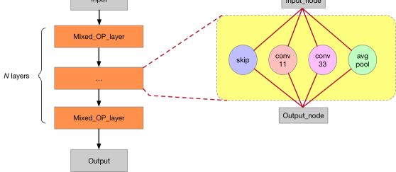
In the context of differentiable NAS, a supernet would contain multiple candidate operations on each edge as shown in Figure 1. Operation scoring functions assign a score to rank operations and select the best one. In this section, we empirically quantify the effectiveness of existing operation scoring methods in differentiable NAS, with a specific focus on DARTS (Liu, Simonyan, and Yang 2019) and the recently-proposed DARTS-PT (Wang et al. 2021). Concretely, we view these scoring functions as proxies for final subnetwork accuracies and we evaluate them on that basis to quantify how well these functions perform. We challenge many assumptions made in previous work and show that we can outperform existing methods with lightweight alternatives.

3.1 Operation Scoring Preliminaries

Figure 1: Visualization of perturbation and discretization of an edge in a supernet. Middle: a supernet is composed of three edges $\{e^{(i)}\}_{i=1,2,3}$, each consisting of three possible operations $\{o^{(i)}\}_{i=1,2,3}$ which are applied in parallel to the same input. Left: edge $e^{(2)}$ is perturbed by removing $o^{(1)}$ from the set of candidate operations assigned to this edge. Right: the same edge $e^{(2)}$ is discretized with operation $o^{(1)}$ by removing all other candidate operations leaving $o^{(1)}$ as the only choice left.

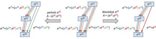
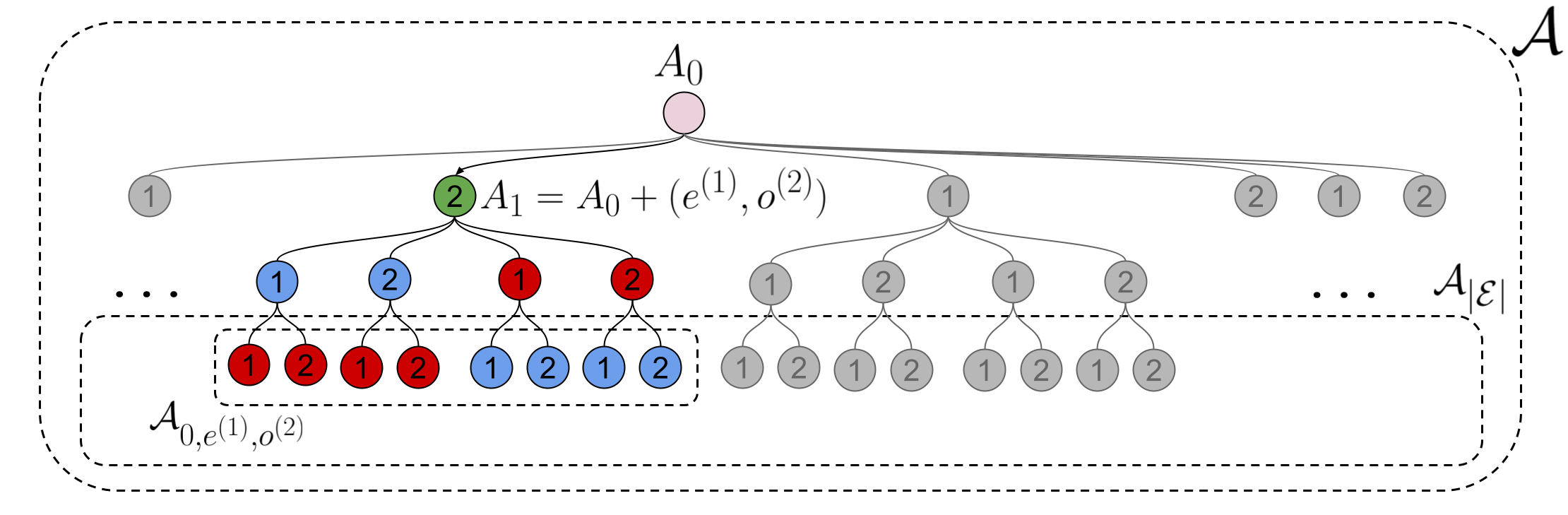
For a supernet $A$ we want to be able to start discretizing edges in order to derive a subnetwork. When discretizing we replace an edge composed of multiple candidate operations and their respective (optional) architectural parameters $\alpha$ with only one operation selected from the candidates. We will denote the process of discretization of an edge $e$ with operation $o$, given a model $A$, as: $A+(e,o)$. Analogously, the perturbation of a supernet $A$ by removing an operation $o$ from an edge $e$ will be denoted as $A-(e,o)$. Figure 1 illustrates discretization and perturbation. Furthermore, we will use $\mathcal{A}$, $\mathcal{E}$ and $\mathcal{O}$ to refer to the set of all possible network architectures, edges in the supernet and candidate operations, respectively. More details about notation can be found in Appendix A.1.

NAS can then be performed by iterative discretization of edges in the supernet, yielding in the process a sequence of partially discretized architectures: $A_{0},A_{1},...,A_{|\mathcal{E}|}$, where $A_{0}$ is the original supernet, $A_{|\mathcal{E}|}$ is the final fully-discretized subnetwork (result of NAS), and $A_{t}$ is $A_{t-1}$ after discretizing a next edge, i.e., $A_{t}=A_{t-1}+(e_{t},o_{t})$ where $t$ is an iteration counter. The problem of finding the sequence of $(e_{t},o_{t})$ that maximizes the performance of the resulting network $A_{|\mathcal{E}|}$ has an optimal substructure and can be reduced to the problem of finding the optimal policy $\pi:\mathcal{A}\times\mathcal{E}\rightarrow\mathcal{O}$ that is used to decide on an operation to assign to an edge at each iteration, given current model (state). This policy function is defined by means of an analogous scoring function $f:\mathcal{A}\times\mathcal{E}\times\mathcal{O}\rightarrow\mathbb{R}$, that assigns scores to the possible values of the policy function, and then taking $\operatorname*{arg\,max}$ or $\operatorname*{arg\,min}$ over $f$, depending on the type of scores produced by $f$.

We begin by defining the optimal scoring function that we will later use to assess the quality of different empirical approaches. For a given partially-discretized model $A_{t}$, let us denote the set of all possible fully-discretized networks that can be obtained from $A_{t}$ after a next edge $e$ is discretized with an operation $o$ as $\mathcal{A}_{t,e,o}$. Our optimal scoring function can then be defined as:

$$\pi_{\text{best-acc}}(A_{t},e)=\operatorname*{arg\,max}_{o\in\mathcal{O}_{e}}\max_{A_{|\mathcal{E}|}\in\mathcal{A}_{t,e,o}}V^{*}(A_{|\mathcal{E}|})$$ (1)

where $V^{*}$ is the validation accuracy of a network after converged (we will use $V$ to denote validation accuracy without training), and $\mathcal{O}_{e}\subseteq\mathcal{O}$ is the subset of candidate operations that are considered for edge $e$. It is easy to see that this policy meets Bellman’s principle of optimality (Bellman 1957) – the definition follows directly from it and therefore is the optimal solution to our problem. However, it might be more practical to consider the expected achievable accuracy when an operation is selected, instead of the best. Therefore we define the function $\pi_{\text{avg-acc}}$:

$$\pi_{\text{avg-acc}}(A_{t},e)=\operatorname*{arg\,max}_{o\in\mathcal{O}_{e}}\mathop{\mathbb{E}}_{A_{|\mathcal{E}|}\in\mathcal{A}_{t,e,o}}V^{*}(A_{|\mathcal{E}|})$$ (2)

In practice, we are unable to use either $\pi_{\text{best-acc}}$ or $\pi_{\text{avg-acc}}$ since we would need to have the final validation accuracy $V^{*}$ of all the networks in the search space. Here we consider the following practical alternatives from DARTS (Liu, Simonyan, and Yang 2019) and the recent DARTS-PT (Wang et al. 2021):

$$\pi_{\text{darts}}(A_{t},e) =\operatorname*{arg\,max}_{o\in\mathcal{O}_{e}}\alpha_{e,o}$$ (3)

$$\pi_{\text{disc-acc}}(A_{t},e) =\operatorname*{arg\,max}_{o\in\mathcal{O}_{e}}V^{*}(A_{t}+(e,o))$$ (4)

$$\pi_{\text{darts-pt}}(A_{t},e) =\operatorname*{arg\,min}_{o\in\mathcal{O}_{e}}V(A_{t}-(e,o))$$ (5)

where $\alpha_{e,o}$ is the architectural parameter assigned to operation $o$ on edge $e$ as presented in DARTS (Liu, Simonyan, and Yang 2019). $\pi_{\text{disc-acc}}$ uses accuracy of a supernet after an operation $o$ is assigned to an edge $e$ – this is referred to as “discretization accuracy” in DARTS-PT and is assumed to be a good operation scoring function (Wang et al. 2021), it could approximate $f_{\text{avg-acc}}$. $\pi_{\text{darts-pt}}$ is the perturbation-based approach used by DARTS-PT – it is presented as a practical and lightweight alternative to $\pi_{\text{disc-acc}}$ (Wang et al. 2021).

Zero-Cost Operation Scoring. We argue that the scoring functions 3-5 are merely proxies for the best achievable accuracy (Eq. 1). As such, we see an opportunity to use a new class of training-free proxies that are very fast to compute and have been shown to work well within multi-trial NAS, albeit not in differentiable NAS, nor within large search spaces. We present the following scoring functions that use a zero-cost proxy $S$ instead of validation accuracy when discretizing an edge or perturbing an operation. Note that the supernet is randomly-initialized and untrained.

$$\pi_{\text{disc-zc}}(A_{t},e) =\operatorname*{arg\,max}_{o\in\mathcal{O}_{e}}S(A_{t}+(e,o))$$ (6)

$$\pi_{\text{zc-pt}}(A_{t},e) =\operatorname*{arg\,min}_{o\in\mathcal{O}_{e}}S(A_{t}-(e,o))$$ (7)

In the rest of this paper, we consider the following proxies that have been proposed in recent zero-cost NAS literature: grad_norm (Abdelfattah et al. 2021), snip (Lee, Ajanthan, and Torr 2019), grasp (Wang, Zhang, and Grosse 2020), synflow (Tanaka et al. 2020), fisher (Theis et al. 2018), zen_score (Lin et al. 2021), tenas (Chen, Gong, and Wang 2021) and nwot (Mellor et al. 2021). Detailed metrics descriptions are included in Appendix A.2. Note that in most existing work (Abdelfattah et al. 2021; Mellor et al. 2021), zero-cost metrics are not used to score operations but to select architectures based on their end-to-end scores, their effectiveness on operation selection remains to discover, and we are going to show that building operation scoring function and algorithm upon on them is trivial, while TE-NAS (Chen, Gong, and Wang 2021) also uses them to score operations. However, as opposed to selecting the optimal operations (via either discretization or perturbation), the tenas metric is used to iteratively prune the weakest operations from a supernet (Chen, Gong, and Wang 2021).

3.2 Empirical Analysis on Operation Scoring

In this subsection, we investigate the performance of different operation scoring methods. Because we want to compare with the optimal best-acc and avg-acc, we conduct experiments on two popular NAS benchmarks: NAS-Bench-201 (Dong and Yang 2020) and NAS-Bench-1Shot1 (Zela, Siems, and Hutter 2020). In the following, we discuss our findings using NAS-Bench-201, while results on NAS-Bench-1Shot1 can be found in Appendix A.10. We conduct our investigation in two settings, initial and progressive. The first setting compares operation scoring functions while making their first decision (iteration 0) during NAS. The second, progressive, setting takes into account retraining of a partially discretized supernet $A_{t}$ and a subsequent rescoring of operations, that might occur between iterations of different algorithms that we consider like darts-pt (Wang et al. 2021).

Figure 2: Left: Rank correlation coefficient between different operation scoring metrics at the first iteration of NAS. Right: Rank correlation coefficient of different operation scoring functions vs. best-acc when invoked iteratively for each edge. In iteration $i$, only edge $i$ is discretized then all scores for all operations on the remaining edges is computed and correlated against best-acc.

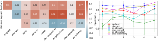
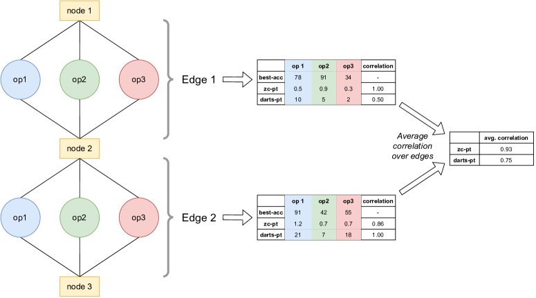
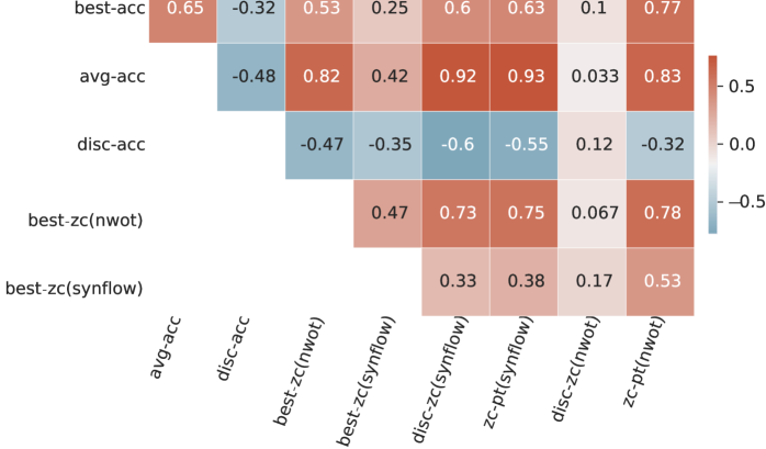
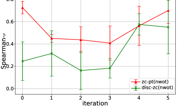
Initial Operation Scoring. For the supernet $A_{0}$ we compute the operation scores for all operations on all edges, at the first iteration (iteration 0) of NAS, that is, $f(A_{0},e,o)\,\,\forall\,\,e\in\mathcal{E},\,\,o\in\mathcal{O}_{e}$. In our first experiment, we collect the scores produced by different scoring methods, per operation, per edge, then compute the Spearman rank correlation for operations on each edge, and finally average the rank correlation coefficient over all edges (details of our experiments and illustrative examples are provided in Appendix A.3). The resulting averaged rank correlation is indicative of how well an operation scoring method would do when making the first discretization decision, relative to a perfect “oracle” search. We plot the rank correlation coefficients in Figure 2, showing many surprising findings. First, the original darts $\alpha$ score is weakly and inversely correlated with the oracle scores, further supporting arguments in prior work that this is not an effective operation scoring method. Second, disc-acc is inversely correlated to best-acc. This refutes the claim in the DARTS-PT paper that disc-acc is a reasonable operation score (Wang et al. 2021) – these findings are aligned with prior work that has already shown that the supernet accuracy is unrelated to the final subnetwork accuracy (Li et al. 2020). Third, the darts-pt score does not track disc-acc, in fact, it is inversely-correlated to it as well, meaning that the darts-pt score is not a good approximation of disc-acc. However, darts-pt is weakly correlated to the “oracle” best-acc and avg-acc scores which supports (empirically) why it works well. Fourth, tenas (Chen, Gong, and Wang 2021), which also utilizes training-free operation scoring, performs fairly well, with Spearman-$\rho=$0.44, but still falls short of the performance of the two zc-pt variants ($\rho=$0.77 and 0.63). Finally, our zc-pt, when using either synflow or nwot metric, is strongly correlated with both the best-acc and avg-acc metrics, indicating that there could be huge promise when using this scoring function within NAS. Note that disc-zc, in particular when using nwot metric, is only weakly correlated with the oracle scores, suggesting that perturbation is a more robust scoring paradigm than discretization. We provide more analysis on disc-zc vs. later, and compare NAS results when using either scoring method in Appendix A.6.

In Table 1, we show the discovered NAS-Bench-201 architecture when applying the seven scoring functions (Eq. (1) – (7)) for operation selection on all edges. As expected, best-acc chooses the best subnetwork, while avg-acc selects a very good model but not the best one, likely due to the large variance of accuracies in NAS-Bench-201. zc-pt(nwot) selected one of the top models in NAS-Bench-201 as expected from the strong correlation with the oracle best-acc function; while tenas selected a good model, in the top 15% of the NAS-Bench-201 dataset, commensurate with the average correlation shown in Figure 2. The remaining operation scoring functions failed to produce a good model in this experiment, suggesting that these metrics do not make a good initial choice of operations at iteration 0 of differentiable NAS. A similar analysis of NAS-Bench-1shot1 search space can be found in Appendix A.10. We provide a more detailed look into the failures of certain scoring methods below.

Table 1: Model selected based on maximizing each operation strength independently.

	best-acc	avg-acc	disc-acc	darts-pt
Avg. Error1 [%]	5.63	6.24	13.55	19.43
Rank in NAS-Bench-201	1	166	12,744	13,770
	zc-pt(nwot)	disc-zc(nwot)	darts	tenas
Avg. Error1 [%]	5.81	22.96	45.7	7.19
Rank in NAS-Bench-201	14	14,274	15,231	1,817

• Computed as the average of all available seeds for the selected model in NAS-Bench-201 CIFAR-10 dataset.

Analysis of the darts-pt and disc-acc scoring. As mentioned before, our zc-pt operation scoring function outperforms both darts-pt and disc-acc, despite the latter methods relying directly on accuracy. This may sound counter-intuitive, but it becomes clearer if we note that the accuracy used by these methods (supernet accuracy) is not directly relevant to the NAS objective (subnet accuracy). Regarding darts-pt, we argue that the unrolled estimation performed by a supernet, as described by (Wang et al. 2021), might lead to the observed preference towards selecting skip connections (see Table A12). This is because under this hypothesis, convolutional operations on an edge perform only refinement of the input, while most of the information is carried directly from the input through a skip connection. Therefore, it can be expected that removal of the skip connection should have much severe effects on the supernet’s performance. More information can be found in Appendix A.3.

Regarding disc-acc, we perform an additional case study of how the supernet’s accuracy changes after discretizing an edge with different operations, as a function of training epochs. The experiment details are in Appendix A.3. From the results we can see that as retraining progresses, lighter operations (none in particular) converge much faster than heavy, but potentially more meaningful, operations like conv_1x1. What is more, even after sufficiently long training, all choices converge to roughly the same point. We argue that this is caused by the fact that in the early NAS iterations the supernet is heavily overparamtrized, which hinders our ability to faithfully measure each operation’s contribution based simply on the accuracy of the supernet.

Analysis of the zc-pt and disc-zc scoring. We further perform detailed experiments on comparing both pertubation and discretization policies, especially when using nwot zero-cost metric. Specifically, we create a toy model that allows us to observe how disc-zc(nwot) and zc-pt(nwot) behave in a simplified setting, as we vary the model’s depth. We observe that while both approaches behave similarly when a network is shallow, as we increase its depth disc-zc quickly degrades and becomes biased towards selecting skip connection, which is not the case for zc-pt. This suggests that nwot might in fact prefer shallower networks – however, unlike discretization, perturbation paradigm does not introduce the ability to reduce the supernet’s depth (as long as each edge includes at least two meaningful operations among their candidates), which seems to robustify nwot significantly. More detailed can be found in Appendix A.4.

While the above signals some major weaknesses of different proxies used in differentiable NAS, when used to perform initial scoring of operations, it’s worthwhile to further analyze them in the progressive setting which would show what happens in later NAS iterations.

Progressive Operation Scoring. Until now, we have only investigated the performance of operation scoring functions in the first iteration of NAS. This approach is relevant for methods like DARTS, where operation scoring function $f$ does not depend on $A_{t}$ in any way (only $A_{0}$), but is not truly representative of other methods that work iteratively. Because of that, we extend our analysis to investigate what happens in later iterations of NAS. To do that, we calculate the correlation of scoring functions in the progressive setting by performing the following steps: (1) score operations on all undiscretized edges, (2) discretize edge $i$, (3) retrain for 5 epochs (darts-pt and disc-acc only), (4) increment $i$ and repeat from step 1 until all edges are discretized. At each iteration $i$, we calculate the scores for the operations on all remaining undiscretized edges and compute their Spearman-$\rho$ rank correlation coefficients with respect to best-acc. This is plotted in Figure 2, averaged over 4 seeds.

Our results confirm many of our initial (iteration-0) analysis. zc-pt(nwot) continues to be the best operation scoring function, and darts-pt is the second-best, improving in correlation from 0.4 to 0.6 between the first and last iterations, indeed showing that retraining and/or progressive discretization helps. However, disc-acc continues to be unrepresentative of operation strength even when used in the iterative setting. This is not what we expected, especially in the very last iteration when disc-acc is supposed to match a subnetwork exactly. As Figure 2 shows, the variance in the last iteration is quite large – we believe this happens because we do not train to convergence every time we discretize an edge, and instead we only train for 5 epochs. Our progressive analysis provided further empirical evidence that supernet discretization accuracy should not be used as a proxy for subnetwork accuracy, contradicting (Wang et al. 2021). However, we have confirmed that darts-pt does in fact improve when retraining is performed between NAS iterations, but could still be improved upon with zc-pt – it performed exceptionally well as a proxy for accuracy and has the potential to make differentiable NAS both much faster and of higher accuracy.

4 Zero-Cost-PT Neural Architecture Search

Based on our analysis of operation scoring, in this section, we propose a NAS algorithm called Zero-Cost-PT using zero-cost perturbation and perform ablation studies to find the best set of heuristics for our NAS methodology, including: edge discretization order, number of search and validation iterations, and the choice of the zero-cost metric.

4.1 Architecture Search with Zero-cost Proxies

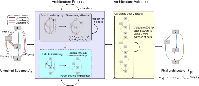
Our algorithm contains two stages: architecture proposal and validation. It begins with an untrained supernet $A_{0}$ which contains a set of edges $\mathcal{E}$, the number of proposal iterations $\mathtt{N}$, and the number of validation iterations $\mathtt{V}$. In each proposal iteration $i$, we discretize the supernet $A_{0}$ based on our proposed zero-cost-based perturbation function $f_{\text{zc-pt}}$ that achieved promising results in the previous section. After all edges have been discretized, the final architecture is added to the set of candidates and we begin the process again for $i+1$ starting with the original $A_{0}$. After $\mathtt{N}$ candidate architectures have been constructed, the validation stage begins. We score the candidate architectures again using a selected zero-cost metric (the same which is used in $f_{\text{zc-pt}}$), but this time computing their end-to-end score rather than using the perturbation paradigm. We calculate the zero-cost metric for each subnetwork using $\mathtt{V}$ different minibatches of data. The final architecture is the one that achieves the best total score during the validation stage. The full algorithm is outlined as Algorithm 1 in Appendix A.5 and the flowchart of our algorithms is in Figure 3 . Our algorithm contains four main hyperparameters: $\mathtt{N}$, $\mathtt{V}$, ordering of edges to follow when discretizing, and the zero-cost metric to use ($S$). In the following we present detailed ablations to decide on the best possible configuration of these.

Figure 3: Flowchart of the proposed Zero-Cost-PT algorithm.

Table 2: Comparison in test error (%) with SOTA perturbation-based and zero-cost NAS on NAS-Bench-201 (Best in red, 2nd best in blue. Same for all following tables).

Method	CIFAR-10	CIFAR-100	ImageNet-16
Zero-Cost-PT${}_{\texttt{random}}$ with different proxies (Section 4.2)
tenas (Chen, Gong, and Wang 2021)	70.07±39.87	83.04±31.93	90.57±17.21
fisher (Theis et al. 2018)	10.64±1.27	38.48±1.96	82.85±12.63
grad_norm (Abdelfattah et al. 2021)	10.55±1.11	38.43±2.10	80.71±12.10
grasp (Wang, Zhang, and Grosse 2020)	9.81±3.42	36.52±6.33	64.27±8.82
snip (Lee, Ajanthan, and Torr 2019)	8.32±2.02	34.00±4.03	65.35±11.04
zen_score1 (Lin et al. 2021)	6.24±0.00	28.89±0.00	58.56±0.00
synflow1 (Tanaka et al. 2020)	6.24±0.00	28.89±0.00	58.56±0.00
nwot (Mellor et al. 2021)	5.97±0.17	27.47±0.28	53.82±0.77
Baselines and SOTA approaches (Section 5.1)
Random	13.39±13.28	39.17±12.58	66.87±9.66
DARTS	45.70±0.00	84.39±0.00	83.68±0.00
DARTS-PT 1	11.89±0.00	45.72±6.26	69.60±4.40
DARTS-PT (fix $\alpha$) 1, 2	6.20±0.00	34.03±2.24	61.36±1.91
NASWOT(synflow) 3	6.54±0.62	29.53±2.13	58.22±4.18
NASWOT(nwot) 3	7.04±0.80	29.97±1.16	55.57±2.07
TE-NAS	6.10±0.47	28.76±0.56	57.62±0.46
Zero-Cost-Disc(nwot (Mellor et al. 2021))	6.22±0.84	28.18±2.01	55.14±1.77

• Only 1 model was selected across all 4 seeds in both cases.

• Results on CIFAR-10 taken from (Wang et al. 2021). Results on other datasets computed using official code in (Wang et al. 2021) across 4 seeds.

• Using N=1000 for both proxies and averaged over 500 runs as in (Mellor et al. 2021).

4.2 Ablation Study

We conduct ablations of the proposed Zero-Cost-PT approach on NAS-Bench-201 (Dong and Yang 2020). More results on additional NAS search spaces and benchmarks are reported later in Section 5 and Appendix A.7. NAS-Bench-201 constructed a unified cell-based search space, where each architecture has been trained on three different datasets, CIFAR-10, CIFAR-100 and ImageNet-16-120. In our experiments, we take a randomly initialised supernet for this search space and apply our Zero-Cost-PT algorithm to search for architectures without any training. We search with four random seeds (0, 1, 2, 3) and report the average and standard deviation of test errors of the obtained architectures. All searches are performed on CIFAR-10, and obtained architectures are then additionally evaluated on the other two datasets.

Different Zero-cost Metrics. Since our focus is to understand how existing zero-cost metrics can be successfully applied to a large-space NAS, we begin our investigation by analysis how different metrics behave when used in the proposed combination with perturbation-based search. It is also worth noting that our formulation and analysis are general and can be extended to new zero-cost proxies that may emerge in the future. For now we only consider random edge discretization order (Zero-Cost-PT${}_{\texttt{random}}$), and more details on edge discretization order will be presented later. Table 2 compares the average test errors of architectures selected by different proxies on NAS-Bench-201. We see that nwot, synflow and zen_score perform considerably better across the three datasets than the others, where nwot offers around 0.27% improvement over synflow. On the other hand, we notice tenas fails in this case, as the metric was designed for pruning operations rather than selecting them (more details are discussed in Appendix A.6). Other than that, even the naive grad_norm outperforms the state-of-the-art DARTS-PT on this benchmark. This confirms it is the appropriate combination of zero-cost metrics and perturbation-based NAS paradigms as in Zero-Cost-PT that could become promising proxies to the actual trained accuracy. We also observed that the ranking of those metrics are quite stable on the three datasets (descending order in terms of error as in Table 2), indicating that architectures discovered by our Zero-Cost-PT have good transferability. In particular nwot consistently performs best, reducing test errors on all datasets by a considerable margin.

Figure 4: (left) Accuracy vs. score of architectures discovered on CIFAR-10 by Zero-Cost-PT with different $\mathtt{N}$. (right) Accuracy distribution of discovered architectures with different $\mathtt{N}$ and $\mathtt{V}$.

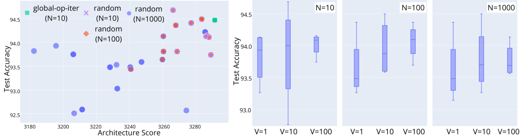
Architecture Proposal vs. Validation. We then study the impact of different architecture proposal iterations $\mathtt{N}$ and validation iterations $\mathtt{V}$ when Zero-Cost-PT uses nwot metric and random edge discretization order. Intuitively, larger $\mathtt{N}$ leads to more architecture candidates being found, while $\mathtt{V}$ indicates the amount of data used to rank the search candidates. As shown in Figure 4, we see larger $\mathtt{N}$ does lead to more architectures discovered, but not proportional to the value of $\mathtt{N}$ on NAS-Bench-201 space. For $\mathtt{N}$=100 we discover 27.8 distinct architectures on average, but when increased to $\mathtt{N}$=1000 the number only roughly doubles. We also see that even with $\mathtt{N}$=10, Zero-Cost-PT${}_{\texttt{random}}$ can already discover top models in the space, demonstrating desirable balance between search quality and efficiency. On the other hand, as shown in Figure 4, larger $\mathtt{V}$ tends to reduce the performance variance, especially for smaller $\mathtt{N}$. This is also expected as more validation iterations could stabilise the ranking of selected architecture candidates, helping Zero-Cost-PT to retain the most promising ones with a manageable overhead of $\mathtt{V}$ mini-batches.

To further justify our finding on NAS-Bench-201, we performed similar ablations on DARTS-CNN space. We study the impact of different architecture proposal iterations N and validation iterations V when Zero-Cost-PT uses random as the search order and nwot metric. The further experiment details are in Appendix A.7

We first consider an extreme case, setting architecture proposal iteration N=1, where Zero-Cost-PT only proposes one architecture candidate (with random edge discretization order), and with no validation stage performed. And then, in order to maximize the performance of our method, we balance exploration (higher N + random edge order) and exploitation (higher V) in the searching and validation phases respectively.

Admittedly, the interplay between those two phases is crucial for our method. To further showcase how the validation phase complements the searching phase, we run additional ablations on the DARTS CNN space with N=10 and V={1,10,100}, the results are shown in Table 3. The results are consistent with what is shown in the NAS-Bench-201: higher V produces better results on average but does not affect the best case that much (the best model is still upper-bounded by what was found with N=1).

Table 3: Ablation overview, the performance of Zero-Cost-PT${}_{\texttt{random}}$ with N={1, 10}, V={0, 1, 10, 100}, nwot metric on DARTS CNN space.

[]       N       V       Test Error(%)       Avg.       Best       1       0       2.81_±0.29       2.43       10       1       2.93_±0.14       2.65       10       2.88_±0.14       2.65       100       2.64_±0.16       2.43

Edge Discretization Order. Finally, we investigate how different edge discretization orders may impact the performance of our Zero-Cost-PT approach, when the best performing nwot metric, $\mathtt{N}$=10 and $\mathtt{V}$=100 are used. We consider the following edge discretization orders:

• fixed: discretizes the edges in a fixed order, where our experiments discretize from the input towards the output;

• random: discretizes the edges in a random order;

• global-op-iter: iteratively evaluates $S(A-(e,o))$ for all operations on all edges in $\mathcal{E}$, selects the edge $e$ containing the operation $o^{\ast}$ with globally best score. Discretizes $e$ with $o^{\ast}$, then repeats to decide on the next edge (re-evaluating scores) until all edges have been discretized;

• global-edge-iter: similar to the above but iteratively selects edge $e$ from $\mathcal{E}$ based on the average score of all operations on each edge;

• global-op-once: only evaluates $S(A-(e,o))$ for all operations once to obtain a ranking order of the operations and decide the edge order upfront based on it, then starts following the algorithm as usual, calculating scores of operations at each edge iteratively;

• global-edge-once: similar to the above but uses the average score of operations on edges to obtain the edge discretization order.

Table 4: Comparison with s SOTA differentiable NAS methods on the DARTS CNN search space (CIFAR-10).

Method	Error [%]		Params	Cost
	Avg.	Best	[M]	[GPU-days]
DARTS (Liu, Simonyan, and Yang 2019)	3.00±0.14	-	3.3	0.4
SDARTS-RS (Chen and Hsieh 2020)	2.67±0.03	-	3.4	0.4
SGAS (Li et al. 2020)	2.66±0.24	-	3.7	0.25
DARTS-PT (Wang et al. 2021)	2.61±0.08	2.48	3.0	0.8
DARTS-PT${}_{+\texttt{none}}$1	2.73±0.13	2.67	3.2	0.8
TE-NAS (Chen, Gong, and Wang 2021)	2.63±0.064	-	3.8	0.05
max-param-random	2.94±0.098	2.83	5.14	-
NASWOT(2500)	2.99±0.22	2.66	-	0.018
NASWOT(20000)	2.73±0.09	2.58	-	0.083
NASWOT(50000)	2.72±0.09	2.52	-	0.208
Zero-Cost-EVO	2.94±0.14	2.72	-	0.018
Zero-Cost-PT${}_{\texttt{synflow}}$	3.88±0.56	3.38	5.1	-
Zero-Cost-PT${}_{\texttt{zen\_score}}$	3.06±0.31	2.68	2.9	-
Zero-Cost-PT${}_{\texttt{random}}$	2.64±0.16	2.43	4.7	0.018
Zero-Cost-PT${}_{\texttt{global-op-iter}}$	2.62±0.09	2.49	4.6	0.17

• Results obtained by re-enabling none operation in DARTS-PT (Wang et al. 2021).

Table. 5 shows the performance of and # of perturbations required by our Zero-Cost-PT approach when using different edge discretization order, under nwot metric, with $\mathtt{N}=10$ and $\mathtt{V}=100$.

We observe that global-op-iter consistently performs best across all three datasets since it iteratively explores the search space of remaining operations while greedily selecting the current best. On the other hand, we see that the performance of global-op-once is inferior since it determines the order of perturbation by assessing the importance of operations once and for all at the beginning, which may not be appropriate as discretization continues. We observe similar behaviour in global-edge-iter and global-edge-once, both of which use the average importance of operations on edges to decide search order, leading to suboptimal performance. It is also worth pointing out that fixed performs relatively well comparing to the other variants, offering comparable performance with random. This shows that Zero-Cost-PT is generally robust to the edge discretization order. In the following experiments, we use Zero-Cost-PT with random order with a moderate setting in architecture proposal iterations ($\mathtt{N}$=10) to balance exploration and exploitation during the search, while maintaining efficiency.

Table 5: Test error (%) of Zero-Cost-PT when using different search orders on NAS-Bench-201.

Search Order1	# of Perturbations2	C10	C100	ImageNet-16
fixed	$|\mathcal{O}||\mathcal{E}|$	5.98±0.50	27.60±1.63	54.23±0.93
global-op-iter	$\frac{1}{2}|\mathcal{O}||\mathcal{E}|(|\mathcal{E}|+1)$	5.69±0.19	26.80±0.51	53.64±0.40
global-op-once	$2|\mathcal{O}||\mathcal{E}|-|\mathcal{O}|$	6.30±0.57	28.96±1.66	55.04±1.47
global-edge-iter	$\frac{1}{2}|\mathcal{O}||\mathcal{E}|(|\mathcal{E}|+1)$	6.23±0.45	28.42±0.59	54.39±0.47
global-edge-once	$2|\mathcal{O}||\mathcal{E}|-|\mathcal{O}|$	6.30±0.57	28.96±1.66	55.04±1.47
random	$|\mathcal{O}||\mathcal{E}|$	5.97±0.17	27.47±0.28	53.82±0.77

• All methods use nwot metric, $\mathtt{N}$=10 search iterations and $\mathtt{V}$=100 validation iteration.

• Number of perturbations per search iteration.

5 Results

Table 6: Comparison with SOTA differentiable NAS methods on the DARTS CNN search space (ImageNet).

Method	Error [%]		Params	Cost
	Top-1	Top-5	[M]	[GPU-days]
DARTS (Liu, Simonyan, and Yang 2019)	26.7	8.7	4.7	0.4
SDARTS-RS (Chen and Hsieh 2020)	25.6	8.2	-	0.4
DARTS-PT (Wang et al. 2021)	25.5	8.0	4.6	0.8
PC-DARTS (Xu et al. 2020)	25.1	7.8	5.3	0.1
SGAS (Li et al. 2020)	24.1	7.3	5.4	0.25
TE-NAS(C10) (Chen, Gong, and Wang 2021)	26.2	8.3	6.3	0.05
TE-NAS (Chen, Gong, and Wang 2021)	24.5	7.5	5.4	0.17
Zero-Cost-PT1 (best)	24.4	7.5	6.3	0.018
Zero-Cost-PT1 (4 seeds)	24.6±0.13	7.6±0.09	6.3	0.018

• We use the same training pipeline from DARTS (Liu, Simonyan, and Yang 2019).

In this section, we perform extensive empirical comparisons of Zero-Cost-PT with the state-of-the-art differentiable and zero-cost NAS algorithms on a number of search spaces. Due to space limit, in the following, we present results on NAS-Bench-201 (Dong and Yang 2020), DARTS CNN space (Liu, Simonyan, and Yang 2019) and the practical large search space MobileNet-like space. Results on NAS-Bench-1shot1 (Zela, Siems, and Hutter 2020), NAS-Bench-Macro (Su et al. 2021) and the four DARTS subspaces S1-S4 (Zela et al. 2020), together with detailed experimental settings and more baselines are in Appendix A.9 A.10, A.11, A.12, .

5.1 Tabular NAS Benchmarks

Table 2 shows the average test error (%) of the competing approaches and our Zero-Cost-PT on the three datasets in NAS-Bench-201. Here we include the naive random search and original DARTS as baselines, and compare our approach with the recent zero-cost NAS algorithm NASWOT (Mellor et al. 2021), TE-NAS (Chen, Gong, and Wang 2021), as well as the perturbation-based NAS approaches DARTS-PT and DARTS-PT (fix $\alpha$) (Wang et al. 2021). As in all competing approaches, we perform a search on CIFAR-10 and evaluate the final model on all three datasets. We see that on all datasets, our Zero-Cost-PT (with nwot) consistently offers superior performance, especially on CIFAR-100 and ImageNet-16. On the other hand, the best existing perturbation-based algorithm, DARTS-PT (fix $\alpha$), fails on those two datasets, producing suboptimal results with small improvements compared to random search, suggesting that architectures discovered by DARTS-PT might not transfer well to other datasets. TE-NAS is second best on CIFAR but as we show in the later section, performance deteriorates on larger datasets like ImageNet.

We compare the performance of Zero-Cost-DISC and our proposed Zero-Cost-PT on NAS-Bench-201 (Dong and Yang 2020), as shown in Table 2. We see that discretization (Zero-Cost-DISC) results in inferior performance compared to the proposed perturbation-based approach (Zero-Cost-PT) on all datasets, confirming our previous analysis on their correlations with the oracle metric.

5.2 DARTS CNN Search Space

We use the same settings as in DARTS-PT (Wang et al. 2021), but instead of pre-training the supernet and fine-tuning it after each perturbation, we take an untrained supernet and directly perform our algorithm as in Section 4.1. Additional details, baselines, ablations and discovered architectures can be found in Appendix A.7, A.9, and A.13.

Results on CIFAR-10. As shown in Table 4 the proposed Zero-Cost-PT approaches can achieve a much better average test error than the DARTS and are comparable to its newer variants SDARTS-RS (Chen and Hsieh 2020) and SGAS (Li et al. 2020) at a much lower searching cost (especially when using random edge ordering). There is a significant search cost reduction compared to DARTS-PT. While DARTS-PT needs to perform retraining between iterations, Zero-Cost-PT only evaluates the score of the perturbed supernet with zero-cost proxies ($S_{\texttt{nwot}}$), requiring less than a minibatch of data. Note that here the cost of Zero-Cost-PT reported in Table 4 is for $\mathtt{N}$=10 ( random edge discretization order), and thus a single proposal iteration only takes about a few minutes to run. The global-op-iter variant offers better performance with lower variance compared to random but incurs slightly heavier computation.

Different Zero-cost Searching Approaches.

We additionally compare our Zero-Cost-PT to several alternative ways of performing zero-cost NAS, to further show its efficiency in utilising zero-cost proxies and assert its efficiency as a searching methodology.

We start with the simplest baseline of maximizing number of parameters – this is based on the observation that our method tends to select slightly larger models than some of the baselines in Table 4 and Table 6. We include details in the Appendix A.7 and summarize our finding here. Overall, the test error (%) of this baseline is 2.93_±0.23 (avg.) and 2.78 (min), vs. our 2.64_±0.16 (avg.) and 2.43 (min). This confirms that simply selecting models with maximum FLOPs/Params is not an appropriate searching methodology in general, and that our methods performs more meanigngful architecture selection than simply maximising model size.

In Section 5.1, we compared our method to sampling-based zero-cost NAS in Table 2 (see NASWOT lines). Our results are empirically better on all three datasets. Additionally, our method computes the operation score per edge in a supernet, whereas the sampling-based approach computes the end-to-end network score. The relationship between the number of subnetworks and the number of operations is exponential. Therefore, we anticipate having to sample exponentially many networks in sample-based NASWOT (Mellor et al. 2021) compared to our proposed Zero-Cost-PT.

In order to extend the comparison between zero-cost NAS (NASWOT) and our Zero-Cost-PT to the DARTS CNN search space, we have conducted further experiments similar to NASWOT on NAS-Bench-201, the details of these experiments can be found in Appendix A.7 and the results are presented in Table 4. In summary, for a similar time budget to ours (25 min), the average performance of the baseline is actually closer to the random search (3.29_±0.15) (Liu, Simonyan, and Yang 2019) than to our method, with significant variance.

In addition to the random sampling baseline presented above, here we further extend our study by performing an evolution-based search for a model maximizing the nwot metric (instead of sampling randomly as above) which is then trained. We denote this baseline as Zero-Cost-EVO. We allow a similar search budget (2500 sample size, $\sim$25min on a single 2080ti GPU), and follow the same settings as in our experiments (searching with 4 random seeds, each of the discovered models is trained with 4 random seeds). The results are shown in Table 4. We can see that when given a similar search budget, the evolution-based search performs significantly worse than our Zero-Cost-PT (avg. of 2.94 vs. 2.64), confirming the efficacy of the proposed NAS algorithm.

Results on ImageNet. Table 6 shows the ImageNet classification accuracy for architectures searched on CIFAR-10. Our Zero-Cost-PT${}_{\texttt{random}}$ algorithm is able to find architectures with a comparable accuracy much faster than previous work, further reinforcing its efficacy in this setting. While TE-NAS results on CIFAR-10 were very close to Zero-Cost-PT, a much larger difference is observed on ImageNet with an accuracy drop of 1.8 pp and a search time that is $\sim$2.5$\times$ slower than Zero-Cost-PT.

5.3 MobileNet-like Search Space

It is well known that most of the existing NAS algorithms designed for MobileNet-like perform constrained NAS. However, our method has not been designed for such a context. To the best of our knowledge, the necessity to consider both scores of operations and their potential contribution to the sum of #FLOPS/Params of the final model would result in a potentially NP-hard problem. Therefore, we do not enforce such constraints at this point, as it is less relevant to the proposed approach.

Results on ImageNet. Table 7 shows the performance (error %) of the architectures discovered by the proposed Zero-Cost-PT algorithm on ImageNet, using a MobileNet-like search space from ProxylessNAS (Cai, Zhu, and Han 2019), we, therefore, compare only to results using the same setting. We see that compared to the existing train-based approaches, our approach allows for finding even better models, but also larger ones, much faster (at least $190\times$ speed up). Please note, that because our method performs unconstrained NAS, unlike existing baselines, the results should not be interpreted as being objectively better. Instead, we simply use them as reference points to put our results in perspective – the goal was to show that our method works well in this type of search space and the results support this claim; as expected, more accurate models, but with a larger footprint, can be found faster compared to the constrained baselines.

Table 7: Comparison on MobileNet search space (ImageNet)

[] Architecture Error [%] Params Cost Top-1. Top-5 [M] [GPU-days] MobileNet-V3(1.0)(Howard et al. 2019) 24.8 - 5.3 288 GreedyNAS (You et al. 2020) 25.1 - 3.8 7.6 SPOS (Guo et al. 2019) 25.3 - - 12.4 ProxylessNAS (GPU) (Cai, Zhu, and Han 2019) 24.9 7.5 7.1 8.3 Zero-Cost-PT(best) 23.6 6.8 8.0 0.041 Zero-Cost-PT(avg) 23.8_±0.08 6.93_±0.09 8.1 0.041

6 Conclusion

In this paper, we formalized the implicit operation scoring proxies that are present within differentiable NAS algorithms to both analyze existing methods and propose new ones. We showed that lightweight operation scoring methods based on zero-cost proxies empirically outperform existing operation scoring functions. We also found that perturbation is more effective than discretization when scoring an operation, leading to our lightweight NAS algorithm, Zero-Cost-PT. Our approach outperforms the best available differentiable architecture search in terms of searching time and accuracy even in very large search spaces.

Appendix A Appendix

A.1 Additional Details on Notations

All sets are denoted with stylised capital letters using latex’s mathcal font. Letters denoting elements of different sets use the same letters as the sets, e.g. $e\in\mathcal{E}$, $A\in\mathcal{A}$, etc. For any element, we use subscript for indexing iterations of the discretization process – e.g., $A_{0}$ is a network architecture at the beginning of iteration 0, $e_{2}$ is an edge that is being investigated in iteration 2, etc. To identify different elements in any other context we use superscript, e.g. $e^{(1)}$ might denote the first edge in a supernet, which might be different from $e_{1}$ which denotes the edge that is first going to be dicretized following a relevant discretization order.

To better understand meaning of each used symbol, consider a hypothetical supernet with 3 edges – $e^{(1)},e^{(2)},e^{(3)}$ – repented by different colors (green, blue and red, respectively) and 2 candidate operations – $o^{(1)},o^{(2)}$ – represented by different numbers (1 and 2). Figure A1 visualises the entire space related to the decision process that is happening in order to perform NAS in this setting, including the first discretization step $A_{1}=A_{0}+(e_{0},o_{0})$, where $e_{0}=e^{(1)},o_{0}=o^{(2)}$, and the related set of all achievable fully-discretized models $\mathcal{A}_{0,e_{0},o_{0}}$ – a concept central to our definition of the optimal scoring function.

Figure A1: Visualisation of the searching tree related to a hypothetical supernetwork with 3 nodes (represented by different colors) and 2 candidate operations (represented by different numbers). The root node of the tree represents a full supernetwork. Each descendant node represents a non-unique network architecture obtained by discretizing an edge identified by the color of the node, with an operations encoded by a number in the node, given an architecture represented by a parent node. $\mathcal{A}$ is the set of all possible architectures, including the supernet $A_{0}$, partially-discretized networks like $A_{1}$ and fully-discretized networks. The set of all fully-discretized networks is additionally denoted as $\mathcal{A}_{|\mathcal{E}|}$, and the set of all fully-discretized networks that are achievable after operation $o^{(2)}$ is assigned to edge $e^{(1)}$, given $A_{0}$, is labeled as $\mathcal{A}_{0,e^{(1)},o^{(2)}}$. The arrow from $A_{0}$ to $A_{1}$ represents a possible first step during the discretization process which closes all grayed-out configurations. While performing NAS, at each tree level we need to decide which edge to follow; this is achieved by assigning scores to all/some of the edges that we are willing to consider in each iteration using different scoring functions which are the main focus of our analysis in Section 3.

A.2 More on Zero-Cost Proxies

This section provides more details on the zero-cost proxies considered in our analysis (Section 3), ablation study (Section 4) and experiments (Section 5).

grad_norm (Abdelfattah et al. 2021), which is a simple proxy that sums the Euclidean norm of the gradients after a single minibatch of training data.

snip (Lee, Ajanthan, and Torr 2019), which approximates the change in loss when a specific parameter is removed:

$$\mathtt{snip}:\mathcal{S}_{p}(\theta)=\left\lvert\frac{\partial\mathcal{L}}{\partial\theta}\odot\theta\right\rvert,\,\,\,\,\,\,\,\,\$$ (8)

grasp, which approximates the change in gradient norm (instead of loss) when a parameter is pruned in their grasp objective:

$$\mathtt{grasp}:\mathcal{S}_{p}(\theta)=-(H\frac{\partial\mathcal{L}}{\partial\theta})\odot\theta,\,\,\,\,\,\,\,\,\$$ (9)

synflow, which generalized the above two so-called synaptic saliency scores and proposed a modified version which avoids layer collapse when performing parameter pruning:

$$\mathtt{synflow}:\mathcal{S}_{p}(\theta)=\frac{\partial\mathcal{L}}{\partial\theta}\odot\theta$$ (10)

where $\mathcal{L}$ is the loss function of a neural network with parameters $\theta$, $H$ is the Hessian, $\mathcal{S}_{p}$ is the per-parameter saliency and $\odot$ is the Hadamard product.

nwot (Mellor et al. 2021), which scores an untrained network by examining the the overlap of activations between data points:

$$s=\log|\mathbf{K}_{H}|,\;\;\;\mathbf{K}_{H}=\begin{pmatrix}N_{A}-d_{H}(\mathbf{c}_{1},\mathbf{c}_{1})&\cdots&N_{A}-d_{H}(\mathbf{c}_{1},\mathbf{c}_{N})\\ \vdots&\ddots&\vdots\\ N_{A}-d_{H}(\mathbf{c}_{N},\mathbf{c}_{1})&\cdots&N_{A}-d_{H}(\mathbf{c}_{N},\mathbf{c}_{N})\end{pmatrix}$$ (11)

where $N_{A}$ is the number of rectified linear unites, and $d_{H}(\mathbf{c}_{1},\mathbf{c}_{1})$ is the Hamming distance between two binary codes, induced by the untrained network at two inputs.

tenas (Chen, Gong, and Wang 2021), which uses the spectrum of the neural tangent kernel (NTK) $\kappa_{\mathcal{N}}$ and the number of linear regions in the input space $\hat{R}_{\mathcal{N}}$ to rank architectures, which are defined as

$$\kappa_{\mathcal{N}}=\frac{\lambda_{0}}{\lambda_{m}},\;\;\;\hat{R}_{\mathcal{N}}\simeq\mathop{{}\mathbb{E}}_{\theta}R_{\mathcal{N},\theta}$$ (12)

where $\lambda_{0}$, $\lambda_{m}$ are the eigenvalues of the NTK.

zen_score (Lin et al. 2021), which is a re-scaled version of $\Phi$-score (by the product of BN layers’ variance statistics), measuring the expressivity of a neural network by its expected Gaussian complexity:

$$\Phi(f)=\log\mathop{{}\mathbb{E}}_{\boldsymbol{x},\theta}\|\nabla_{\boldsymbol{x}}f(\boldsymbol{x}|\boldsymbol{\theta})\|_{F}$$ (13)

where $f(\cdot)$ is a vanilla neural network.

A.3 More on Operation Scoring

This section provides more experimental details and examples of our analysis of the operation scoring functions introduced in Section 3.

Detailed Scoring Methodology

As discussed in Section 3.2, our analysis on the on the initial operation scoring aims to investigate how well an operation scoring method can perform when making the first discrietization decision, with respect to the perfect search (the best-acc approach). Here “the first discrietization decision” is made at the first iteration (iteration 0) of a progressive operation selection algorithm, and in our experiment we compute the score for all operations on an edge and later average across all edges to account for random selection of the first edge. Concretely, we compute the score per operation across all edges, then compute the Spearman rank correlation for operations on each edge. After that, we average the rank correlation coefficient over all edges.

Consider the example shown in Figure A2. Suppose we have a supernet with just two edges as in Figure A2. In this case, an operation scoring function should pick just one operation per edge. For a given operation scoring function, we compute the scores for each operation on each edge. Then for each edge, we compute the rank correlation of the oracle scores (best-acc or avg-acc) against the scores from the other operation scoring function (e.g. zc-pt or darts-pt). We then average their correlation coefficient across all edges in a supernet to get an average correlation for each operation scoring function. The resulting average rank correlation is indicative of how well a given operation scoring function (starting with a random edge) would do when making the first discretization decision, relative to the oracle search.

Figure A2: An example showing how correlations of different proxies are computed in our analysis on initial operation scoring in Section 3.2

Experimental Details

Here, we provide some additional experimental details for the data presented in Section 3. The following list describes how we compute each operation score.

• best-acc: To get the score for an operation $o$ on a specific edge $e$, we find the maximum test accuracy of all NAS-Bench-201 architectures with $(o,e)$.

• avg-acc: Same as best-acc but we average all NAS-Bench-201 architecture test accuracies instead of finding the maximum.

• disc-acc: We discretize one edge $e$ by selecting an operation $o$, then we train for 5 epochs and record the supernet accuracy – this is used as the score for $(o,e)$.

• darts-pt: We perturb one edge with one operation $A-(e,o)$ and record the validation accuracy. For perturbation-based scoring functions, we multiply the score by $-1$ before computing correlations.

• disc-zc: We discretize one edge $e$ by selecting an operation $o$ and then compute the zero-cost metric.

• zc-pt: We perturb one edge with one operation $A-(e,o)$ and compute the zero-cost metric. For perturbation-based scoring functions, we multiply the score by $-1$ before computing correlations.

• darts: We record the value of the architecture parameters $\alpha$ after 60 epochs of training the supernet.

• tenas: We perturb one edge with one operation $A-(e,o)$ and compute the $\kappa_{\mathcal{N}}$ and the $\hat{R}_{\mathcal{N}}$ (number of linear regions). Then we rank $\kappa_{\mathcal{N}}$ ascendingly and descendingly rank the $\hat{R}_{\mathcal{N}}$. At last, we add those two ranks together to get the final ranks of the operations. We multiply the score by $-1$ before computing correlations.

Detailed Operation Scores

Table A12 (at the end of this Appendix) shows all operation scores at iteration 0. This data was used to compute Spearman-$\rho$ in Figure 2. Note that we compute Spearman-$\rho$ per edge and average over all edges – this summarizes how well each score tracks our “oracle” best-acc score.

Additional Analysis on darts-pt and disc-acc

Darts-pt makes an implicit assumption that changes of accuracy (either due to perturbation or due to discretization followed by fine-tuning) observed in the context of a supernet $A_{t}$ are representative of changes of accuracy in the context of network $A_{|\mathcal{E}|}$. However, especially when $t<|\mathcal{E}|$, these two networks are in fact very different and there is no reason to take this assumption for granted - even though $A_{|\mathcal{E}|}$ can be derived from $A_{t}$ (in general, many networks can be obtained from each other with relatively simple transformations but that does not mean that the same architectural transformations will be beneficial for them).

To be even more specific, let us consider disc-acc and darts-pt separately, as they perform scoring slightly differently and hence suffer from slightly different things. (In the case of darts-pt we will directly rely on the analysis presented in Proposition 1 in the original paper so please refer there for background and details.)

darts-pt begins by training a full supernet - our claim is that this results in an undesired bias as the changes in accuracy of a supernet might not be relevant in the context of a subnet. To justify this claim we begin by quoting implication of Proposition 1 from the DARTS-PT paper (Wang et al. 2021) saying that “in a well-optimized supernet, $x_{c}$ will naturally be closer to $m^{*}$ than $o_{e}(x_{e})$”, where $x_{c}$ is output of a skip-connection component of a mixup operation in a supernet, $o_{e}$ is convolutional operation in the same mixup operation and $m^{*}$ is the optimal feature map for the mixup operation. DARTS-PT uses this to show that because of that magnitude of $\alpha_{skip}$ will be larger and hence selection based on magnitude is biased. However, paradoxically, the solution they proposed suffers from a very similar issue (although maybe in a slightly more indirect way).

Specifically, if we assume that is the optimal output of the mixup operation and the skip connection component is closer to than any convolutional component then it is also expected that perturbing an edge by removing the skip connection will result in the largest deviation from . Consequently, we can expect that the larger the deviation from the optimal output the larger the drop in accuracy, resulting in selection biased towards selecting skip connections. This behaviour is exactly what we observe on NAS-Bench-201 where in the first iteration of NAS darts-pt tends to assign significantly larger scores to skip connections than any other operation (see Table A12). Please note that this analysis does not consider later iterations, so it is still possible that DARTS-PT as a whole works well due to improved performance in later iterations, but at least in early iterations it should be biased towards selecting skip connections (and empirically we can see that the results are actually quite similar to standard darts).

On the other hand, disc-acc considers performance of a supernet after an edge is discretized, thus (locally) avoiding usage of a mixup operation. However, we also observe similar biased behaviour at the early stage of training, i.e., assigning large scores to skip or none operations. We conducted additional experiments on NAS-Bench-201 (iteration 0), following the same setting as DARTS-PT. We first train the full supernet, and then discretize skip, none and conv_1x1 on edge 1 respectively, while keeping other edges unchanged (with mixed operations). We train these three partially discretized supernets for 50 epochs and record validation accuracy. Fig. A3 plots the validation accuracy of the three resulting partially discretized supernets.

Figure A3: Validation accuracy of three partially discretized supernets at iteration 0 trained on NAS-Bench-201, with none, skip and conv_1x1 operation selected on edge 1 respectively.

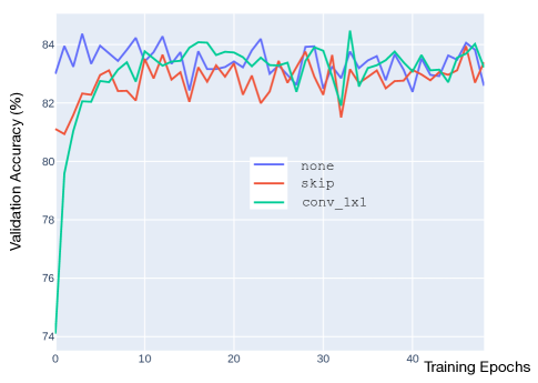
As we can see, at the early stage of training, the supernets with none or skip operations selected have much higher accuracy than that of conv_1x1, this is due to the well-known difficulties in training full supernets (see e.g. TE-NAS (Chen, Gong, and Wang 2021) 3.2.1) Note that although DARTS-PT defines discretization accuracy as the accuracy after convergence, its algorithm only trains for 5 epochs due to the cost (we mention this in Appendix A.3.2). In that case, disc-acc would very likely make wrong decisions as to which operation to choose. On the other hand, as training continues, the ranking of these three operations computed by disc-acc (discretization accuracy) is still unstable, which may again lead to suboptimal decisions. As mentioned above, such bias towards skip or none in early iterations would result in inferior performance, e.g. weaker correlation with the oracle, as we demonstrated in the paper.

A.4 Additional Analysis on zc-pt vs. disc-zc

As shown in Section 3.2, the proposed zc-pt operation scoring function, when using either synflow or nwot metrics, demonstrates strong correlations with the oracle best-acc and avg-acc metrics. However, we also observe that disc-zc, in particular when nwot metric is used, is only weakly or inversely correlated with the oracle. This suggests that perturbation is more robust than discretization, when combined with the zero-cost metric nwot. In this section, we attempt to explain this observation with further analysis.

As discussed in Section 3.1, our scoring functions disc-zc and zc-pt use a zero-cost proxy $S$ instead of validation accuracy when discretizing an edge or perturbing an operation. As shown by (Abdelfattah et al. 2021; Mellor et al. 2021), the zero-cost score of a final architecture $S(A_{|\mathcal{E}|})$ correlates to the model accuracy after full training $V^{*}(A_{|\mathcal{E}|})$, subject to certain levels of fidelity. In that sense, during iterative NAS process like the one in our work, a well performing zero-cost operation scoring function should lead to models $A_{|\mathcal{E}|}$ with high zero-cost scores $S(A_{|\mathcal{E}|})$, which have better chances to achieve high accuracy. To assess the capability of different zero-cost scoring functions in tracking the final architecture score $S(A_{|\mathcal{E}|})$, here we define another oracle score function $\pi_{\text{best-zc}}$:

$$\pi_{\text{best-zc}}(A_{t},e)=\operatorname*{arg\,max}_{o\in\mathcal{O}_{e}}\max_{A_{|\mathcal{E}|}\in\mathcal{A}_{t,e,o}}S(A_{|\mathcal{E}|})$$ (14)

which is the best achievable zero-cost score of all possible architectures under metric $S$ with $(o,e)$ being selected. Fig. 4(a) shows the correlation of different scoring functions at iteration 0 evaluated on NAS-Bench-201. First, we see that synflow metric, when combined with both discretization (disc-zc(synflow)) and perturbation (zc-pt(synflow)) paradigms, correlates well with best-acc and best-zc. On the other hand, for nwot metric, there is a big discrepancy between the two paradigms. Specifically, while zc-pt(nwot) shows the strongest overall performance in tracking both best-acc and best-zc its counterpart, disc-zc(nwot), does not correlates well with neither, further confirming our findings in Section 3.2. Similarly in the progressive setting, as shown in Fig. 4(a), disc-zc(nwot) is weakly/inversely correlated with best-zc(nwot), explaining its inferior NAS performance (more details shown later by the Zero-Cost-DISC baseline in Appendix A.6). Similar analysis on NAS-Bench-1Shot1 (Zela, Siems, and Hutter 2020) can be found in Appendix A.10.

(a)

(b)

Figure A4: (a) Spearman’s rank correlation coefficient of different zero-cost operation scoring metrics with the oracle metrics at the first iteration of NAS. (b) Rank correlation coefficient of disc-zc(nwot) and zc-pt(nwot) vs. best-zc(nwot) when invoked iteratively for each edge.

Figure A5: A simplified supernetowrk with $N$ layers of mixed operations: {skip, conv_1x1, conv_3x3, avg_pooling}.

Figure A6: Rank correlation coefficient of disc-zc(nwot) and zc-pt(nwot) vs. best-zc(nwot) (at iteration 0) with supernetworks of different number of layers $N$.

Table A1: Number of times different operations were selected by disc-zc(nwot), zc-pt(nwot) and best-zc(nwot) at iteration 0 in NAS-Bench-201.

	disc-zc(nwot)	zc-pt(nwot)	best-zc(nwot)
none	0	0	0
skip	5	1	1
conv_1x1	1	2	4
conv_3x3	0	3	1
avg_pooling	0	0	0

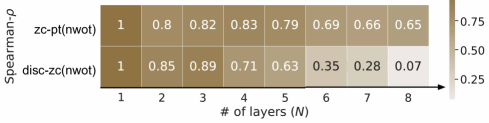
To further investigate the different behaviour of disc-zc(nwot) and zc-pt(nwot), let us consider a simplified supernetwork as in Fig. A5. The supernetwork has a chain structure of $N$ layers of mixed operations, with four candidate operations: {skip, conv_1x1, conv_3x3, avg_pooling}. We vary the number of layers $N$ and calculate Spearman’s rank correlation coefficient of disc-zc(nwot) and zc-pt(nwot) vs. best-zc(nwot) at iteration 0 (note that here we compute the scores for all operations on an edge and then average across all edges, as explained later in Appendix A.3).

Figure A6 shows the trend of the ranking correlation coefficient of different approaches as supernet depth $N$ increases. It is straightforward to see that in the simplest case when $N$ = 1, all three approaches make the same decision. As $N$ increases, zc-pt(nwot) keeps tracking best-zc(nwot) well, while on the other hand, disc-zc(nwot) performs particularly bad. For instance, with the $N$ = 8 layer supernet, disc-zc(nwot) only weakly/inversely correlates with best-zc(nwot) (rank correlation coefficient 0.07), while zc-pt(nwot) remains strongly correlated (rank correlation coefficient 0.65).

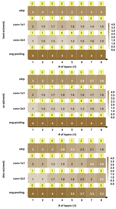
We further plot the average rank of each candidate operation determined by best-zc(nwot), disc-zc(nwot) and zc-pt(nwot) for supernets with different $N$, and the numbers of a particular operation being selected by different approaches when making the decision at iteration 0 (highlighted in yellow) in Figure A7. Clearly, we notice that as $N$ increases disc-zc(nwot) tends to erroneously favour the skip operation, e.g. for the $N$ = 8 layer supernet, in 5 out of 8 times disc-zc(nwot) chose skip as the best operation. This is also evidenced by the the increase of the average rank of skip determined by disc-zc(nwot), resulting in the other operations such as conv_1x1 and conv_3x3 being muted in the NAS process. On the other hand, we see that zc-pt(nwot) does not suffer from this problem, where the selection of operations is well aligned with the oracle best-zc(nwot).

Table A2: Distribution of operations in the 10 final architectures (N = 10 in our Zero-Cost-PT algorithm) generated by disc-zc(nwot) and zc-pt(nwot), compared with the best 10 architectures in the NAS-Bench-201 space.

	Top 10	disc-zc(nwot)	zc-pt(nwot)
none	0	1	0
skip	12	26	9
conv_1x1	12	14	20
conv_3x3	36	19	31
avg_pooling	0	0	0

With the above analysis on a simplified supernetwork, we assume that it could be the overwhelming selection of skip operation that causes the inferior performance of disc-zc(nwot). Although the mechanism underpinning this observation is different, this also aligns with the well-known robustness issues of DARTS (Zela et al. 2020; Shu, Wang, and Cai 2020; Yu et al. 2020; Wang et al. 2021). We observe similar behaviour of disc-zc(nwot) in NAS-Bench-201 (Dong and Yang 2020) space. As shown in Table A1, at iteration 0, disc-zc(nwot) selected skip operation 5 times. Note that the cell search space of NAS-Bench-201 has 6 edges in total, which means at the first iteration of NAS, disc-zc(nwot) is very likely to choose skip operation to discretize an edge. On the other hand, we see both zc-pt(nwot) and best-zc(nwot) select skip operation for 1 time, which is reasonable.x

We also took a closer look at the final architectures selected by disc-zc(nwot) and zc-pt(nwot) (using N=10 architectural proposal iterations as used in our main paper). As shown in Table A2, the 10 architectures selected by disc-zc(nwot) contain 26 skip operation in total, while zc-pt(nwot) only selected 12. We also see that with the top 10 architectures, i.e. the 10 models with the highest validation accuracy in the entire space contains 12 skip, which is very similar to our zc-pt(nwot). For completeness we provide the list of the 10 architecture selected by disc-zc(nwot) below, where we can clearly see skip operations dominating other choices:

⬇

1[{"id": "0", "genotype": "|nor_conv_3x3~0|+|skip_connect~0|nor_conv_3x3~1|+|skip_connect~0|nor_conv_1x1~1|skip_connect~2|"},

2{"id": "1", "genotype": "|nor_conv_3x3~0|+|skip_connect~0|nor_conv_3x3~1|+|skip_connect~0|nor_conv_3x3~1|skip_connect~2|"},

3{"id": "2", "genotype": "|nor_conv_3x3~0|+|skip_connect~0|nor_conv_3x3~1|+|nor_conv_3x3~0|nor_conv_3x3~1|skip_connect~2|"},

4{"id": "3", "genotype": "|nor_conv_3x3~0|+|skip_connect~0|nor_conv_3x3~1|+|skip_connect~0|nor_conv_1x1~1|skip_connect~2|"},

5{"id": "4", "genotype": "|nor_conv_3x3~0|+|skip_connect~0|nor_conv_1x1~1|+|skip_connect~0|nor_conv_3x3~1|skip_connect~2|"},

6{"id": "5", "genotype": "|skip_connect~0|+|nor_conv_1x1~0|nor_conv_1x1~1|+|nor_conv_3x3~0|skip_connect~1|nor_conv_1x1~2|"},

7{"id": "6", "genotype": "|skip_connect~0|+|nor_conv_3x3~0|nor_conv_1x1~1|+|skip_connect~0|skip_connect~1|nor_conv_1x1~2|"},

8{"id": "7", "genotype": "|nor_conv_3x3~0|+|skip_connect~0|nor_conv_1x1~1|+|skip_connect~0|nor_conv_1x1~1|none~2|"},

9{"id": "8", "genotype": "|skip_connect~0|+|nor_conv_3x3~0|nor_conv_3x3~1|+|skip_connect~0|skip_connect~1|nor_conv_1x1~2|"},

10{"id": "9", "genotype": "|skip_connect~0|+|nor_conv_1x1~0|nor_conv_1x1~1|+|nor_conv_3x3~0|skip_connect~1|nor_conv_1x1~2|"}]

We conduct similar analysis on NAS-Bench-1Shot1 (Zela, Siems, and Hutter 2020) space which does not contain skip in the candidate operation set later in Appendix A.10, and the results further confirm our analysis with the above simplified supernetwork and NAS-Bench-201.

It is also worth pointing out that while the aforementioned observations suggest significant limitations of using discretization paradigm together with the nwot metric, the exact mechanism causing those issues remains an open question. In this work we focus on designing a robust zero-cost operation scoring method (zc-pt) and developing a lightweight but effective NAS algorithm (Zero-Cost-PT) based on that, while we leave the investigation of why other approaches might not work well as future work. We include more discussion on the limitations of our work in Appendix A.14.

Figure A7: Average rank of operations computed by best-zc(nwot) (Top), zc-pt(nwot) (Middle) and disc-zc(nwot) (Bottom) with supernetworks of different number of layers $N$. The number of times where each operation is selected at iteration 0 ($N$ possible edges to discretize in total) are highlighted in yellow boxes above.

A.5 Detailed Zero-Cost-PT Algorithm

Algorithm 1 presents the proposed Zero-Cost-PT algorithm introduced in Section 4.1. It has two stages: searching and validation, where we first iteratively discretize the supernet $A_{0}$ based on zero-cost-based perturbation function $f_{\text{zc-pt}}$ (line 1 - 16), and then in the second stage we use the a zero-cost metric (the same which is used in $f_{\text{zc-pt}}$) to score the candidate architectures (line 17 - 20), and select the one with the highest end-to-end score. In particular for DARTS CNN search space, our Zero-Cost-PT algorithm has an additional topology selection step (line 8 - 14), where for each node in architecture we only retain the top two incoming edges based on the zc-pt score – this is similar to the vanilla DARTS algorithm (Liu, Simonyan, and Yang 2019). For NAS-Bench-201 space our algorithm skips this topology selection step.

Input : An untrained supernetwork $A_{0}$ with set of edges $\mathcal{E}$ and set of nodes $\mathcal{N}$, # of architecture proposal iterations $\mathtt{N}$, # of validation iterations $\mathtt{V}$

Result: A selected architecture $A^{\ast}_{|\mathcal{E}|}$

1 // Stage 1: Architecture Proposal

2 $\mathcal{C}=\varnothing$

3 for $i=1:\mathtt{N}$  do

4       for $t=1:|\mathcal{E}|$  do

5             Select next edge $e_{t}$ using the chosen discretization ordering

6            $o_{t}=\pi_{\text{zc-pt}}(A_{t-1},e_{t})$

7             $A_{t}=A_{t-1}+(e_{t},o_{t})$

8       end for

9      

10      while $|\mathcal{N}|>0$ do // prune the edges of the obtained architecture $A_{|\mathcal{E}|}$

11             Randomly select a node $n\in\mathcal{N}$

12            forall Input edge $e$ to node $n$ do

13                   Evaluate the zc-pt score of the architecture $A_{|\mathcal{E}|}$ when $e$ is removed

14             end forall

15            

16            Retain only edges $e_{n}^{(1)\ast}$, $e_{n}^{(2)\ast}$ with the 1st and 2nd best zc-pt score, and remove $n$ from $\mathcal{N}$

17       end while

18      Add $A_{|\mathcal{E}|}$ to the set of candidate architectures $\mathcal{C}$

19      

20 end for

21

22// Stage 2: Architecture Validation

23for $j=1:\mathtt{V}$  do

24       Calculate $S^{(j)}(A)$ for each $A\in\mathcal{C}$ using a random mini-batch data;

25 end for

26

27Select the best architecture $A^{\ast}_{|\mathcal{E}|}=\operatorname*{arg\,max}_{A\in\mathcal{C}}\sum_{j=1:\mathtt{V}}S^{(j)}(A)$;

Algorithm 1 Zero-Cost Perturbation-based Architecture Search (Zero-Cost-PT)

A.6 Additional Details on NAS-Bench-201 ablations

More Zero-Cost Metrics

We also include the detailed results of using tenas metric (with multiple search seeds) with our Zero-Cost-PT in Table A3. For reproducibility, the discovered architectures are listed below:

⬇

1arch_0=|none~0|+|nor_conv_3x3~0|avg_pool_3x3~1|+|none~0|nor_conv_3x3~1|none~2|

2arch_1=|avg_pool_3x3~0|+|nor_conv_1x1~0|nor_conv_1x1~1|+|none~0|nor_conv_1x1~1|skip_connect~2|

3arch_2=|nor_conv_1x1~0|+|none~0|none~1|+|none~0|none~1|nor_conv_3x3~2|

4arch_3=|skip_connect~0|+|nor_conv_1x1~0|nor_conv_3x3~1|+|none~0|none~1|none~2|

Table A3: Test error (%) of Zero-Cost-PT when using tenas metric on NAS-Bench-201.

Search Seed	C10	C100	ImageNet-16
0	90.00	99.00	99.17
1	10.27	35.14	64.75
2	90.00	99.00	99.17
3	90.00	99.00	99.17
Avg	70.07±39.87	83.04±31.93	90.57±17.21
Best	10.27	35.14	64.75

We see that the tenas metric performs badly in this case, which is consistent with our findings reported in Sec. 3 where the tenas metric achieves lower correlation than synflow or nwot. We also find that the architectures discovered by tenas metric are dominated by the none operations as shown above, resulting in its inferior performance (also see the detailed scores obtained by tenas metric at iteration 0 in Table A12. This shows that as a metric designed to prune operations, tenas fails to work well with iterative discretization (aiming to select the optimal operations), further confirming our argument that it is not a simple task to design a robust zero-cost NAS methodology.

Zero-Cost-DISC Baseline

In Section. 3, we propose two zero-cost operation scoring methods disc-zc and zc-pt (corresponding to policies $\pi_{\text{disc-zc}}$ and $\pi_{\text{zc-pt}}$), and study their correlation with an oracle metric best-acc on NAS-Bench-201 (Dong and Yang 2020). We also provide more in-depth analysis on the two metrics in the above Appendix A.4, and present more results in NAS-Bench-1Shot1 (Zela, Siems, and Hutter 2020) in Appendix A.10.

Table A4: Comparison in test error (%) between zero-cost perturbation-based and discretization-based NAS on NAS-Bench-201.

Method1	CIFAR-10	CIFAR-100	ImageNet-16
Zero-Cost-DISC	6.22±0.84	28.18±2.01	55.14±1.77
Zero-Cost-PT	5.97±0.17	27.47±0.28	53.82±0.77

• We use the same hyperparameter settings as reported in the main paper: N=10, V=100, nwot zero-cost metric and random edge discretization order.

We find that discretization is generally a weaker scoring paradigm than perturbation (especially when nwot is used), as shown by their correlations with respect to the oracle score best-acc and best-zc. To further evaluate the end-to-end NAS performance of discretization vs. perturbation with zero-cost metrics, we consider a baseline named Zero-Cost-DISC, which discretizes the supernet based on $\pi_{\text{disc-zc}}$ instead of $\pi_{\text{zc-pt}}$. Here for simplicity, we only consider nwot metric, and details on how disc-zc computes the operation scores can be found in Appendix A.3. We compare the performance of Zero-Cost-DISC and our proposed Zero-Cost-PT on NAS-Bench-201 (Dong and Yang 2020), as shown in Table A4. We see that discretization (Zero-Cost-DISC) results in inferior performance compared to the proposed perturbation-based approach (Zero-Cost-PT) on all datasets, confirming our previous analysis on their correlations with the oracle metric.

A.7 Additional Ablation Study and Baseline on DARTS CNN Space

Architecture Proposal vs. Validation

Table A5: Detailed performance of Zero-Cost-PT${}_{\texttt{random}}$ with N=1, V=0, nwot metric on DARTS CNN space.

[] S. seed ¹ Test Error (%) Training seed ² Avg. Best 0 1 2 3 0 2.72 2.55 2.83 2.71 1 3.25 3.26 3.28 3.20 2 2.59 2.84 2.59 2.79 3 2.43 2.77 2.52 2.66 2.81_±0.29 2.43

• Random seeds for searching the architectures.

• Random seeds for training the selected architectures.

We conducted an ablation study of our Zero-Cost-PT algorithm on NAS-Bench-201 (Dong and Yang 2020) in Section 4, aiming to decide the best possible configuration of the main hyperparameters of our algorithm: architecture proposal iterations N, validation iterations V, ordering of edges to follow when discretizing, and the zero-cost metric to use. In the following, we present additional ablations on the much larger DARTS CNN space.

We first study the impact of different architecture proposal iterations N and validation iterations V when Zero-Cost-PT uses random as the search order and nwot metric.

As detailed in Algorithm 1, Zero-Cost-PT${}_{\texttt{random}}$ firstly proposes N candidate architectures using the proposed zero-cost perturbation paradigm, which are then evaluated in a lightweight manner during the validation phase to come up with a single outcome of a search. It extends the existing zero-cost NAS approach such as NASWOT (Mellor et al. 2021) by including more sophisticated architecture selection phase based on the combination of zero-cost metrics and perturbations.

We first consider an extreme case, setting architecture proposal iteration N=1, where Zero-Cost-PT only proposes one architecture candidate (with random edge discretization order), and with no validation stage performed. The detailed results are shown in Table A5. As can be seen, the average performance is affected quite significantly. However, the best model still happens to be on-par with our main results. This suggests what has already been mentioned in our main paper, that the searching phase alone tends to “find” many different architectures depending on, broadly speaking, random seed, and this randomness is especially visible in the case of random edge ordering (Figure 4). While the high variance might seem undesired at first, we empirically observe that the higher exploration resulting from it is beneficial for finding some very good models, e.g., global-op-iter discretization order tends to be less sensitive to random seed as it takes away one degree of randomness (edge order), producing more stable results on average, but at the same time limiting its ability to maximize the performance of the best model found (Table 4). In order to maximize the performance of our method, we balance exploration (higher N + random edge order) and exploitation (higher V) in the searching and validation phases respectively.

Admittedly, the interplay between those two phases is crucial for our method. To further showcase how the validation phase complements the searching phase, we run additional ablations on the DARTS CNN space with N=10 and V={1,10,100}, the results are shown in Table A6. The results are consistent with what is shown in the main paper: higher V produces better results on average but does not affect the best case that much (the best model is still upper-bounded by what was found with N=1).

Table A6: Detailed performance of Zero-Cost-PT${}_{\texttt{random}}$ with N=10, V={1, 10, 100}, nwot metric on DARTS CNN space.

[] V S. seed ¹ Test Error (%) Training seed ² Avg. Best 0 1 2 3 1 0 3.08 3.16 3.06 2.96 1 2.74 2.91 2.92 2.92 2 2.96 3.10 3.06 2.90 3 2.86 2.85 2.85 2.65 2.93_±0.14 2.65 10 0 3.08 3.16 3.06 2.96 1 2.74 2.91 2.92 2.87 2 2.77 2.71 2.65 2.76 3 2.83 3.00 2.82 2.87 2.88_±0.14 2.65 100 0 2.86 2.97 2.77 2.82 1 2.51 2.47 2.56 2.43 2 2.74 2.73 2.54 2.62 3 2.43 2.77 2.52 2.64 2.64_±0.16 2.43

• Random seeds for searching the architectures.

• Random seeds for training the selected architectures.

Different Zero-Cost Metrics

Table A7: Test error (%) of Zero-Cost-PT${}_{\texttt{random}}$ when using different zero-cost metrics.

Metric	Average Error	Best Error
synflow1 (Tanaka et al. 2020)	3.88±0.56	3.38
zen_score (Lin et al. 2021)	3.06±0.31	2.68
nwot (Mellor et al. 2021)	2.64±0.16	2.43

• Only 1 model was selected across all 4 random seeds.

We also conducted experiments on DARTS CNN space using different zero-cost metrics with our Zero-Cost-PT algorithm, under the setting of N=10, V=100, and random edge order. In particular, in addition to the nwot metric, we choose the next two best performing metrics, synflow (Tanaka et al. 2020) and zen_score (Lin et al. 2021). We perform search with 4 random seeds, and each discovered model is trained using 4 random seeds respectively. The results are presented in Table A7.

We see that the results are consistent with our analysis on the tabular benchmarks, where nwot outperforms both synflow and zen_score in terms of average and best error by a large margin. In particular, similar to what we observed in NAS-Bench-201, in this case synflow also discovers the same architecture across 4 random seeds, which selects the operation with the most parameters (sep_conv_5x5):

⬇

1Genotype(normal=[["sep_conv_5x5", 0], ["sep_conv_5x5", 1], ["sep_conv_5x5", 1], ["sep_conv_5x5", 2], ["sep_conv_5x5", 2], ["sep_conv_5x5", 3], ["sep_conv_5x5", 3], ["sep_conv_5x5", 4]], normal_concat=[2, 3, 4, 5], reduce=[["sep_conv_5x5", 0], ["sep_conv_5x5", 1], ["sep_conv_5x5", 1], ["sep_conv_5x5", 2], ["sep_conv_5x5", 2], ["sep_conv_5x5", 3], ["sep_conv_5x5", 3], ["sep_conv_5x5", 4]], reduce_concat=range(2, 6))

Maximum-param Baseline

Table A8: Randomly selected architectures with only operation sep_conv_5x5 on DARTS CNN space.

[] S. seed ¹ Test Error(%) Training seed ² Avg. Best 0 1 2 3 0 3.07 2.93 2.89 2.85 2.94_±0.30 2.85 1 2.92 2.93 3.17 3.05 3.02_±0.20 2.92 2 2.98 2.97 2.93 2.90 2.95_±0.06 2.95 3 2.87 2.83 3.02 2.78 2.88_±0.18 2.78

• Random seeds for searching the architectures.

• Random seeds for training the selected architectures.

We create a baseline approach that trains 4 random models with separable convolution 5x5 (the most expensive operation in the DARTS search space) selected everywhere and random connections between layers. The evaluation methodology follows all other experiments, i.e. we have 4 searched models trained 4 times with different training seeds, and we report the average and minimum error.

We also show that the results on simple search spaces like NAS-Bench-201 (NB201), this maximum-param baseline may perform relatively better, e.g. it can find the model with test accuracy of 93.76% (165th position in the ranking), but our method can still do better, discovering the 33rd best model in the search space (test accuracy 94.03%).

In summary, on both NB201 and DARTS space, the proposed combination of the perturbation paradigm with zero-shot proxies does better than the naive usage of the proxies presented in (Abdelfattah et al. 2021; Mellor et al. 2021), as shown in Tables 2, 4, 6. Note that we are better than the plain perturbation-based baseline (Wang et al. 2021) and recent zero-cost NAS (Chen, Gong, and Wang 2021) on NB201 (Table 2), and comparable/better on DARTS and derived subspaces (Table 4 and 6), while being much cheaper to run.

The structures of models are provided as Genotype objects below for reproducibility.

⬇

1random_max_0 = Genotype(normal=[["sep_conv_5x5", 0], ["sep_conv_5x5", 1], ["sep_conv_5x5", 0], ["sep_conv_5x5", 1], ["sep_conv_5x5", 0], ["sep_conv_5x5", 3], ["sep_conv_5x5", 1], ["sep_conv_5x5", 4]], normal_concat=range(2, 6), reduce=[["sep_conv_5x5", 0], ["sep_conv_5x5", 1], ["sep_conv_5x5", 0], ["sep_conv_5x5", 1], ["sep_conv_5x5", 0], ["sep_conv_5x5", 1], ["sep_conv_5x5", 0], ["sep_conv_5x5", 1]], reduce_concat=range(2, 6))

2random_max_1 = Genotype(normal=[["sep_conv_5x5", 0], ["sep_conv_5x5", 1], ["sep_conv_5x5", 0], ["sep_conv_5x5", 2], ["sep_conv_5x5", 0], ["sep_conv_5x5", 2], ["sep_conv_5x5", 1], ["sep_conv_5x5", 4]], normal_concat=range(2, 6), reduce=[["sep_conv_5x5", 0], ["sep_conv_5x5", 1], ["sep_conv_5x5", 0], ["sep_conv_5x5", 1], ["sep_conv_5x5", 0], ["sep_conv_5x5", 1], ["sep_conv_5x5", 0], ["sep_conv_5x5", 1]], reduce_concat=range(2, 6))

3random_max_2 = Genotype(normal=[["sep_conv_5x5", 0], ["sep_conv_5x5", 1], ["sep_conv_5x5", 0], ["sep_conv_5x5", 2], ["sep_conv_5x5", 0], ["sep_conv_5x5", 3], ["sep_conv_5x5", 1], ["sep_conv_5x5", 4]], normal_concat=range(2, 6), reduce=[["sep_conv_5x5", 0], ["sep_conv_5x5", 1], ["sep_conv_5x5", 0], ["sep_conv_5x5", 1], ["sep_conv_5x5", 0], ["sep_conv_5x5", 1], ["sep_conv_5x5", 0], ["sep_conv_5x5", 1]], reduce_concat=range(2, 6))

4random_max_3 = Genotype(normal=[["sep_conv_5x5", 0], ["sep_conv_5x5", 1], ["sep_conv_5x5", 0], ["sep_conv_5x5", 1], ["sep_conv_5x5", 0], ["sep_conv_5x5", 2], ["sep_conv_5x5", 1], ["sep_conv_5x5", 4]], normal_concat=range(2, 6), reduce=[["sep_conv_5x5", 0], ["sep_conv_5x5", 1], ["sep_conv_5x5", 0], ["sep_conv_5x5", 1], ["sep_conv_5x5", 0], ["sep_conv_5x5", 1], ["sep_conv_5x5", 0], ["sep_conv_5x5", 1]], reduce_concat=range(2, 6))

Random Sample Baseline(NASWOT)

In Section 5.1, we compared our method to sampling-based zero-cost NAS in Table 2 (see NASWOT lines). Our results are empirically better on all three datasets. Additionally, our method computes the operation score per edge in a supernet, whereas the sampling-based approach computes the end-to-end network score. The relationship between the number of subnetworks and the number of operations is exponential. Therefore, we anticipate having to sample exponentially many networks in sample-based NASWOT (Mellor et al. 2021) compared to our proposed Zero-Cost-PT.

In order to extend the comparison between zero-cost NAS (NASWOT) and our zero-cost PT to the DARTS CNN search space, we have conducted further experiments, in which we allow NASWOT to sample and score random models from the DARTS search space for a specified amount of samples (2500, 20000, 50000, corresponding to roughly 25min, 2h, and 5h on a single 2080Ti GPU) and the best model, according to the nwot metric, is selected as the result of a search. For each of the three sampling budgets, we run the entire process 4 times using different searching seeds (0-3), thus resulting in 3$\times$4 = 12 final architectures (9 unique ones are selected). Each of the final architectures was then trained 4 times using different training seeds (0-3).

As expected, both the average and best performance of the sample-based zero-cost search increases with more samples. However, the results are visibly behind our proposed method, even for the most expensive searches (5 hours). In addition, we see that increasing the search budget from 2 hours to 5 hours does not result in proportional gains in accuracy, compared to 25min, suggesting diminishing returns. We hypothesize it is related to the mentioned fact that the number of architectures grows exponentially, so we’d need to sample significantly more networks before the probability of hitting a good one increases noticeably. In fact, we find that when increasing the search budget from 20000 to 50000 samples in our experiments, the baseline only gets better results in one out of 4 cases (searching seeds), and in one it actually made the results worse. This further suggests diminishing returns.

A.8 Experiments on DARTS subspaces (S1-S4)

Description of DARTS subspace (S1-S4)

RobustDARTS introduced four different DARTS subspaces to evaluate the robustness of the original DARTS algorithm (Zela et al. 2020). In our work, we validate the robustness of Zero-Cost-PT against some of the more recent algorithms using the same subspaces originally proposed in the RobustDARTS paper (Section A.8). The search spaces are defined as follows:

• in S1 each edge of a supernet consists only of the two candidate operations having the highest magnitude of $\alpha$ in the vanilla DARTS (these operations can be different for different edges);

• S2 only considers two operations: skip_connect and sep_conv_3x3;

• similarly, S3 consists of three operations: none, skip_connect and sep_conv_3x3;

• finally, S4 again considers just two operations: noise and sep_conv_3x3, where noise operation generates random Gaussian noise $\mathcal{N}(0,1)$ in every forwards pass that is independent of the input.

Results on DARTS subspaces (S1 - S4)

It is well known that DARTS could generate trivial architectures with degenerative performance in certain cases. (Zela et al. 2020) have designed various special search spaces for DARTS to investigate its failure cases on them. As in DARTS-PT, we consider spaces S1-S4 to validate the robustness of Zero-Cost-PT in a controlled environment (detailed specifications can be found in Appendix A.8). As shown in Table A9, our approach consistently outperforms the original DARTS, the state-of-the-art DARTS-PT and DARTS-PT(fix $\alpha$) across S1 to S3 on both datasets CIFAR-10 and CIFAR-100, while on SVHN it offers competitive performance comparing the competing algorithms (best in S1, second best in space S2/S3 with .08/.02% gap). This confirms that our Zero-Cost-PT is robust in finding good performing architectures in spaces where DARTS typically fails, e.g. it has been shown (Wang et al. 2021) that in S2 DARTS tends to produce trivial architectures saturated with skip connections. On the other hand, we observe that Zero-Cost-PT doesn’t perform well in search space S4, struggling with operation noise, which simply outputs a random Gaussian noise $\mathcal{N}(0,1)$ regardless of the input. This is expected as score $S(A_{t}-(e,o))$ can be completely random if $o$ = noise. However, since noise operation is not useful in NAS, we are satisfied with the robustness of Zero-Cost-PT.

Table A9: Comparison in test error (%) with state-of-the-art perturbation-based NAS on DARTS spaces S1-S4.

Space	DARTS1	DARTS-PT1		Zero-Cost-PT2
	Best	Best	Best (fix $\alpha$)	Avg.	Best
CIFAR-10
S1	3.84	3.5	2.86	2.75±0.28	2.55
S2	4.85	2.79	2.59	2.49±0.05	2.45
S3	3.34	2.49	2.52	2.47±0.09	2.40
S4	7.20	2.64	2.58	5.23±0.76	4.69
CIFAR-100
S1	29.64	24.48	24.4	22.05±0.29	21.84
S2	26.05	23.16	23.3	20.97±0.50	20.61
S3	28.9	22.03	21.94	21.02±0.57	20.61
S4	22.85	20.80	20.66	25.70±0.01	25.69
SVHN
S1	4.58	2.62	2.39	2.37±0.06	2.33
S2	3.53	2.53	2.32	2.40±0.05	2.36
S3	3.41	2.42	2.32	2.34±0.05	2.30
S4	3.05	2.42	2.39	2.83±0.06	2.79

• Results taken from (Wang et al. 2021).

• Results obtained using random seeds 0 and 2.

A.9 NAS Experimental Details

All searches were run multiple times with different searching seeds (usually 0, 1, 2 and 3). Additionally, each found architecture was trained multiple times using different training seeds – for DARTS the same set of seeds was used for training and searching, for NAS-Bench-201 (NB201) training seeds were taken from the dataset (777, 888 and 999, based on their availability in the dataset). Therefore, for each experiment, we got a total of searching_seeds $\times$ training_seeds accuracy values. Whenever average performance is reported, it is averaged across all obtained results. Similarly, the best values were selected by taking the best single result from the searching and training seeds.

Experimental Details – NAS-Bench-201

Searching was performed using 4 different seeds (0, 1, 2, and 3) to initialise a supernet. Whenever we had to perform training of a supernet during the searching phase (Section 3), we used the same hyperparameters as the original DARTS-PT code used. When searching using our Zero-Cost-PT we used a batch size of 256, N=10, V=100 and S=nwot, unless mentioned otherwise (e.g., during ablation studies). Inputs for calculating zero-cost scores came from the training dataloader(s), as defined for relevant datasets in the original DARTS-PT code (including augmentation). For zero-cost proxies that require a loss function, standard cross-entropy was used. For any searching method, after an algorithm had identified a final subnetwork, we extracted the final architecture and queried the NB201 dataset to obtain test accuracy – one value for each training seed available in the dataset.

All experiments concerning operation scoring (Sections 3 and A.3) used averaged accuracy of models from NB201 for simplicity.

We did not search for architectures targeting CIFAR-100 or ImageNet-16 directly – whenever we report results for these datasets, we used the same architecture found using CIFAR-10.

Experimental Details – DARTS

DARTS experiments follow a similar methodology to NB201. Each algorithm was run with 4 different initialisation seeds for a supernet (0, 1, 2 and 3). When running Zero-Cost-PT, we used the following hyperparameters: the batch size of 64, N=10, V=100 and $S$=nwot. Inputs and the loss function for zero-cost metrics were defined analogically to NB201. We did not run any baseline method on the DARTS search space (all results were taken from the literature), so we did not have to perform any train a supernet. After an algorithm had identified a final subnetwork, we then trained it 4 times using different initialisation seeds again (0, 1, 2 and 3). When training subnetworks, we used a setting aligned with the previous work (Liu, Simonyan, and Yang 2019; Wang et al. 2021).

Unlike NB201, whenever different datasets were considered, (Section A.8) architectures were searched on each relevant dataset directly.

For CIFAR-10 experiments, we trained models using a heavy configuration with init_channels = $36$ and layers = $20$. Models found on CIFAR-100 and SVHN were trained using a mobile setting with init_channels = $16$ and layers = $8$. Both choices follow the previous work (Zela et al. 2020; Wang et al. 2021).

A.10 Additional Experiments on NAS-Bench-1shot1

Figure A8: Spearman’s rank correlation coefficient of different operation scoring metrics with each other at the first iteration of NAS evaluated on NAS-Bench-1Shot1 benchmark.

Figure A9: Rank correlation coefficient of disc-zc(nwot) and zc-pt(nwot) vs. best-zc(nwot) when invoked iteratively for each edge on NAS-Bench-1Shot1 benchmark.

Table A10: Comparison in validation and test error (%) of DARTS (Liu, Simonyan, and Yang 2019) and our Zero-Cost-PT on NAS-Bench-1Shot1 (Zela, Siems, and Hutter 2020) benchmark.

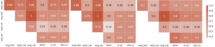
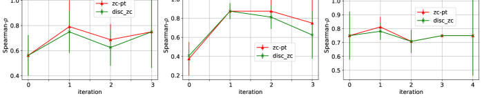
[] Method Space Val Error [%] Test Error [%] Avg. Best Avg. Best DARTS 1 6.11_±0.01 5.90 6.67_±0.08 6.44 Zero-Cost-PT 5.86_±0.05 5.15 6.47_±0.64 5.61 DARTS 2 6.34_±0.05 5.71 6.68_±0.36 6.24 Zero-Cost-PT 5.89_±0.04 5.29 6.65_±0.360 6.15 DARTS 3 6.15_±0.02 5.90 6.64_±0.12 6.5 Zero-Cost-PT 5.90_±0.03 5.31 6.45_±0.31 5.84

In addition to experiments on NAS-Bench-201 (Dong and Yang 2020), we perform additional experiments on NAS-Bench-1shot1 (Zela, Siems, and Hutter 2020) to further evaluate the performance of our Zero-Cost-PT algorithm on relevant NAS benchmarks. When searching using Zero-Cost-PT we used batch size of 256, N=10, V=100 and S=nwot. We first extend our correlation analysis from Section 3 (in particular, the initial operation scoring as in Section 3.2). We compare to DARTS as it is already available in the NB1shot1 codebase . As in Figure A8, the results show that DARTS is surprisingly well-correlated to both best and avg accuracy, in some cases (only in Space 3) even better than our proposed zc-pt. We believe that this is because the search space does not contain skip connections and overall is rather unusual compared to others used with differentiable NAS, so it is possible that it constitutes an edge-case where DARTS performs relatively well. Due to the exact reason, we observe that the performance of disc-zc and zc-pt in tracking the oracle best-zc is very similar, as shown in Figure A9, further confirming our hypothesis about degrading effects of skip connections on disc-zc performance, presented in Appendix A.4.

Table A10 shows the end-to-end NAS results. We can see that our Zero-Cost-PT consistently achieves better performance than DARTS in all 3 spaces, and is able to find better models (best-case scenarios). This confirms our analysis and evaluation presented in the main paper, that Zero-Cost-PT could offer strong NAS performance on various search spaces. We would like to notice that unlike DARTS or NAS-Bench-201, NAS-Bench-1shot1 supernet contains architectural parameters associated with entire connections between cells ($\alpha$ and $\gamma$ in the paper (Zela, Siems, and Hutter 2020)), additionally to the standard ones associated with candidate operations in a single layer ($\beta$ in the paper). What it means for our method is that for those parameters we no longer perturb a single edge of a supernet but rather the entire path, making the setting for our algorithm noticeably different. Further extending our method from operation scoring to path scoring is a very relevant goal for future work.

A.11 Additional Experiments on NAS-Bench-Macro

To further verify the robustness of our Zero-Cost-PT method, we conduct additional experiments on a different type of tabular NAS benchmark, NAS-Bench-Macro (Su et al. 2021). Unlike NAS-Bench-201 (Dong and Yang 2020) and NAS-Bench-1Shot1 (Zela, Siems, and Hutter 2020), NAS-Bench-Macro is a NAS benchmark on macro search space, where candidate blocks are selected during NAS process instead of operations. It consists of 6561 networks with their test accuracies, parameters and FLOPs on CIFAR-10 dataset.

Experimental setting

We follow the same settings as in (Su et al. 2021). The NAS-Bench-Macro search space contains 8 searching layers, each of which has the following 3 candidate blocks:

• Identity: identity connection (encoded as ‘0’);

• MB3_K3: MobileNetV2 block with kernel size 3 and expansion ratio 3 (encoded as ‘1’);

• MB6_K5: MobileNetV2 block with kernel size 5 and expansion ratio 6 (encoded as ‘2’).

The total size of the search space is therefore $3^{8}=6561$, containing 3969 unique architectures. We adopt the same input dimension 32, and run our Zero-Cost-PT NAS algorithm with 4 different random seeds (0, 1, 2, 3) as in all other experiments. We query the discovered architectures and obtain their accuracies, parameters and FLOPs from the benchmark. When searching using Zero-Cost-PT we used batch size of 256, N=10, V=100 and S=nwot (same as in experiments on other tabular NAS benchmarks).

Table A11: Comparison of MCT-NAS (Su et al. 2021) and our Zero-Cost-PT on NAS-Bench-Macro benchmark.

[] Methods Avg. Error [%] Params [M] FLOPs [M] Rank Search Cost ² MCT-NAS ¹ 6.87_±0.253 2.0 85.2 1/6561 0.68 Zero-Cost-PT 7.05_±0.077 2.9 105.7 9/6561 0.05

• Results taken from (Su et al. 2021).

• Averaged over 3 random seeds (used in training) as reported in (Su et al. 2021).

• In GPU hours. Cost for MCT-NAS (Su et al. 2021) is estimated by measuring wall clock time of i) a single epoch supernet training and ii) a single forward pass on validation set with a 2080Ti GPU. No information on search cost is reported on CIFAR-10 in the paper, and the NAS code is not available.

Results

Table A11 compares the NAS results of our Zero-Cost-PT approach and the MCT-NAS algorithm reported on NAS-Bench-Macro (Su et al. 2021). We see that Zero-Cost-PT is able to discover a good architecture (ranked the 9th in all 6561 models), with much less search cost comparing to MCT-NAS reported in NAS-Bench-Macro (Su et al. 2021). Since MCT-NAS did not report search cost on CIFAR-10 dataset, nor release search code, we estimate the cost of MCT-NAS by running i) a single epoch for supernet training, and ii) a single forward pass on validation set with a 2080Ti GPU. We then calculate the total cost according to Algorithm 1 in  (Su et al. 2021) (with 120 epoch of supernet training, 50 search numbers and 256 batch size).

In particular, during search our Zero-Cost-PT selects the same architecture across all 4 seeds (0, 1, 2, 3), which assigns MB6_K5 at every candidate block. Note that the top-1 architecture discovered by MCT-NAS (Su et al. 2021) also tends to choose many MB6_K5 block, with an Identity block selected on the last layer. It is also worth pointing out that in NAS-Bench-Macro benchmark, architectures are only trained for 50 epochs, which may change with further training.

A.12 Experimental Settings on MobileNet-like Search Space

We adopt the same settings as in (Cai, Zhu, and Han 2019) and construct a supernet with 21 choice blocks, and each block has the following 7 alternative operations:

• 3$\times$2 = 6 MobileNet blocks, with 3 different kernel sizes {3, 5, 7} and 2 expansion ratio {3, 6}).

• skip connection.

We follow the previous work (Cai, Zhu, and Han 2019) on this space and search directly on ImageNet dataset (Deng et al. 2009), with input_size = 224. We use 3 different random seeds (0-2) to perform architectures search, and train the discovered final models (3 models searched and trained in total). We use batch-size = 1024 and training was performed on 8 NVIDIA V100 GPUs for 300 epochs, with initial learning rate set to 0.5. We use colour-jitters, random horizontal flip and random crop for data augmentation, set label_smooth = 0.1. All other training setting is identical to ProxylessNAS (Cai, Zhu, and Han 2019).

A.13 Discovered Architectures

Figures A10 and A11 present cells found by our Zero-Cost-PT on the DARTS CNN search space (Section 5.2) when using global-op-iter and random discretization orders, respectively (see Section 4 for the definition of the two discretization orders). Figures A13 through A24 show cells discovered on the four DARTS subspaces and the three relevant datasets (Sections A.8 and A.8). Figure A25 shows architectures found by our Zero-Cost-PT approach on MobileNet-like search space.

A.14 Societal Impact and Limitations

In this paper we study operation scoring in the differentiable NAS context. We propose, evaluate and compare perturbation-based zero-cost operation scoring methods for differentiable NAS building upon recent work on training-free NAS proxies, leading to a lightweight NAS algorithm, Zero-Cost-PT. Our approach outperforms the best available differentiable architecture search in terms of searching time and accuracy even in very large search spaces. As our approach can significantly reduce searching time of NAS, especially for large search spaces, a potential negative societal impact is that GPU time needed to evaluate (training fully) the large number of discovered architectures can be substantial.

One limitation of this work is that our analysis and ablations on operation scoring (Sections 3 and 4) is primarily conducted on tabular NAS benchmarks. Although the superior NAS performance of our Zero-Cost-PT on various larger search spaces indicates that the insights gained from our analysis can indeed transfer to other spaces, we didn’t perform the same analysis on large search spaces such as DARTS due to the prohibitive cost, i.e. computing the correlations with oracle scoring methods will require the full training of all $10^{18}$ models, which is clearly not feasible.

In addition, the proposed approaches and analysis are primarily quantitative and empirical, and in this paper we did not try to provide theoretical explanations to questions revolving around the common problem of explaining why zero-cost proxies work well, or what makes a good zero-cost proxy, or how to select a reasonable zero-cost metric for a specific task. We think that those questions are of great interest to the whole community working on zero-cost proxies in NAS. However, we find them extremely difficult to answer fully at this stage. One of the reasons is simply the fact that those zero-cost proxies work under very different principles, and hence would require different approaches to be analysed – if we strive for an answer that is well-grounded in theory, it will likely be different for proxies like synflow that utilize synaptic-flow and nwot that counts linear regions. At the same time, if we want a theoretically-grounded, analytical answer to those questions, we would need to understand in depth what properties are crucial for those zero-cost proxies to achieve high correlation with post-training accuracy. This naturally involves problems of analysing the (stochastic) training process, its generalization capabilities etc., which are all hard problems and areas of active research in modern ML. Therefore, admittedly in the scope of this paper we do not have conclusive and qualitative answers to those questions.

However, in this paper we show that we can approach the problems from a quantitative perspective. In particular, the investigation in our paper provides one possible way to select (empirically) a reasonable zero-cost metric for a specific context, i.e., we could first conduct quantitative correlation analysis and ablation studies on available tabular NAS benchmarks, and then use the obtained insights (e.g., which metric/hyper-parameters to use) on the actual problem space. We demonstrate that even without qualitative analysis we can still design a robust and sound methodology by following a meticulous and systematic design process with clearly (and correctly) defined quantitative objectives, like those proposed in Section 3. Our hope is that our results will be of interest to parts of the research community and will spur further research into low-cost NAS approaches.

(a) Normal cell

(b) Reduction cell

Figure A10: Cells found by Zero-Cost-PT (global-op-iter discretization order) on the DARTS search space using CIFAR-10.

(a) Normal cell

(b) Reduction cell

Figure A11: Cells found by Zero-Cost-PT (random discretization order) on the DARTS search space using CIFAR-10.

(a) Normal cell

(b) Reduction cell

Figure A12: Cells found by Zero-Cost-PT (random discretization order) on the DARTS search space using ImageNet.

(a) Normal cell

(b) Reduction cell

Figure A13: Cells found by Zero-Cost-PT (random discretization order) on the DARTS-S1 space using CIFAR-10.

(a) Normal cell

(b) Reduction cell

Figure A14: Cells found by Zero-Cost-PT (random discretization order) on the DARTS-S2 space using CIFAR-10.

(a) Normal cell

(b) Reduction cell

Figure A15: Cells found by Zero-Cost-PT (random discretization order) on the DARTS-S3 space using CIFAR-10.

(a) Normal cell

(b) Reduction cell

Figure A16: Cells found by Zero-Cost-PT (random discretization order) on the DARTS-S4 space using CIFAR-10.

(a) Normal cell

(b) Reduction cell

Figure A17: Cells found by Zero-Cost-PT (random discretization order) on the DARTS-S1 space using CIFAR-100.

(a) Normal cell

(b) Reduction cell

Figure A18: Cells found by Zero-Cost-PT (random discretization order) on the DARTS-S2 space using CIFAR-100.

(a) Normal cell

(b) Reduction cell

Figure A19: Cells found by Zero-Cost-PT (random discretization order) on the DARTS-S3 space using CIFAR-100.

(a) Normal cell

(b) Reduction cell

Figure A20: Cells found by Zero-Cost-PT (random discretization order) on the DARTS-S4 space using CIFAR-100.

(a) Normal cell

(b) Reduction cell

Figure A21: Cells found by Zero-Cost-PT (random discretization order) on the DARTS-S1 space using SVHN.

(a) Normal cell

(b) Reduction cell

Figure A22: Cells found by Zero-Cost-PT (random discretization order) on the DARTS-S2 space using SVHN.

(a) Normal cell

(b) Reduction cell

Figure A23: Cells found by Zero-Cost-PT (random discretization order) on the DARTS-S3 space using SVHN.

(a) Normal cell

(b) Reduction cell

Figure A24: Cells found by Zero-Cost-PT (random discretization order) on the DARTS-S4 space using SVHN.

Figure A25: Discovered Architectures in MobileNet-like Search Space

Table A12: Raw values of operation scoring functions at iteration 0 to reproduce Figure 2.

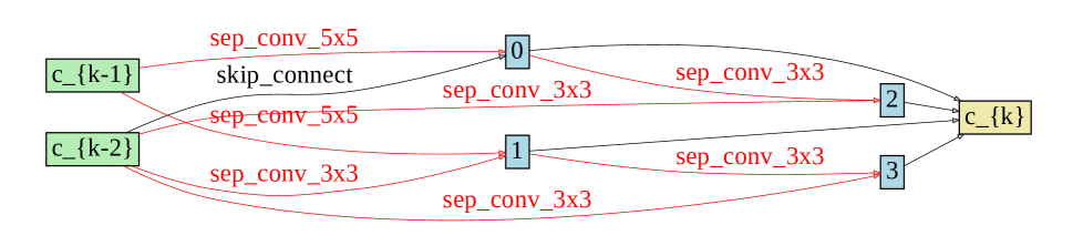
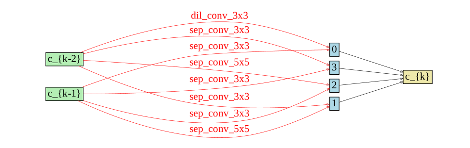
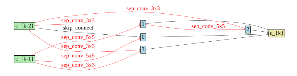
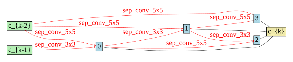
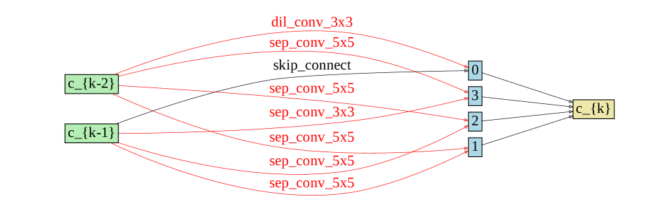
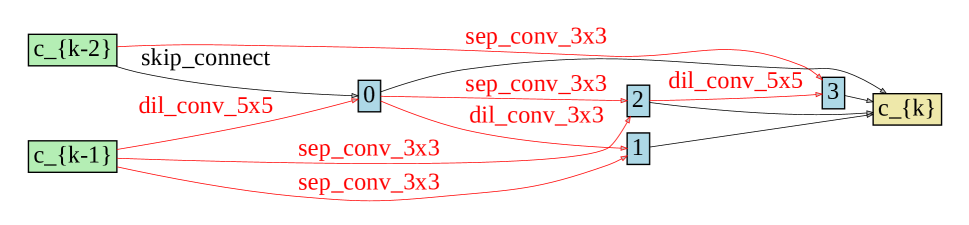
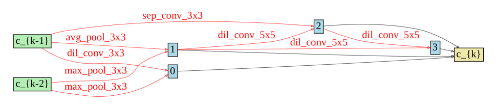
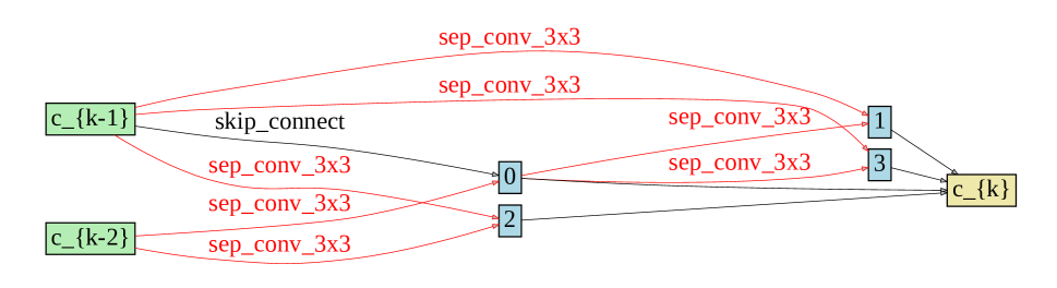
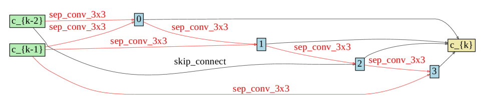
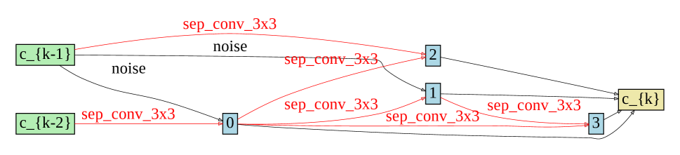
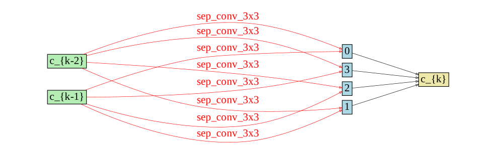
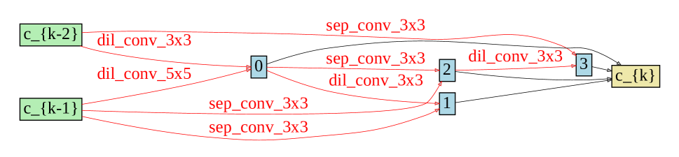
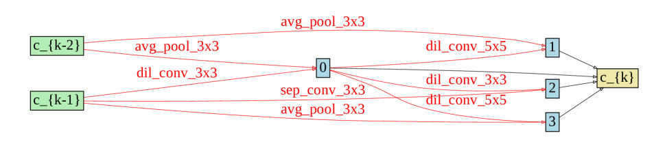
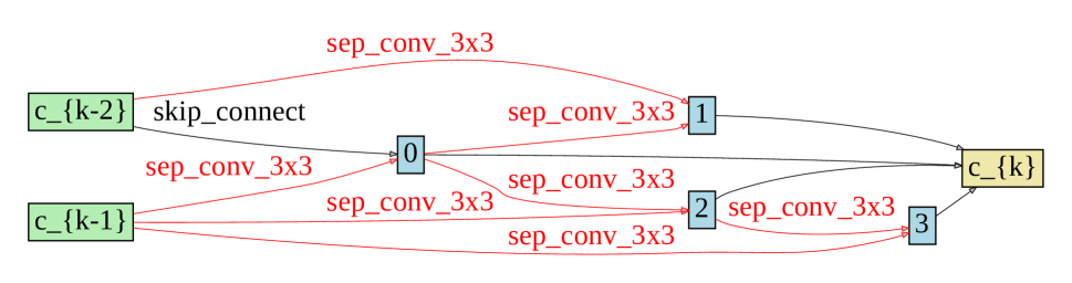
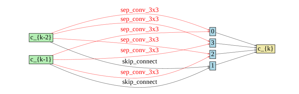
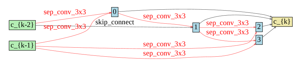
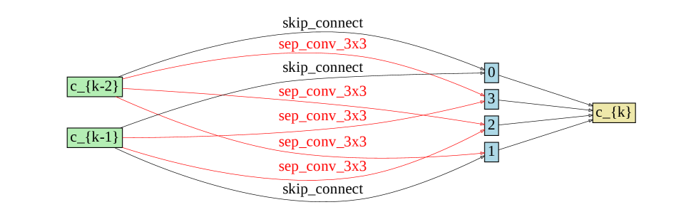
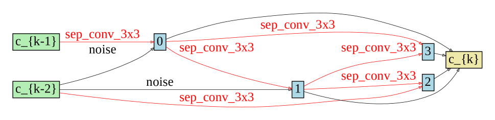
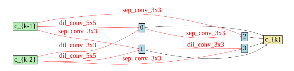
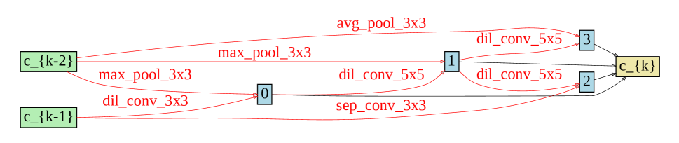
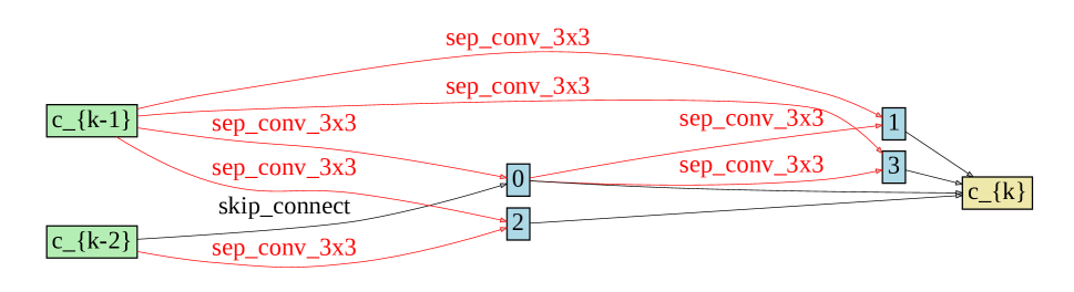
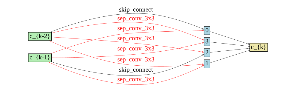
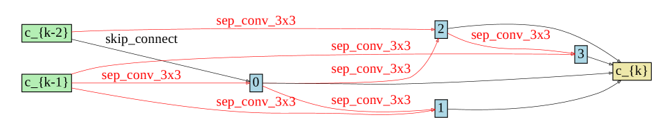
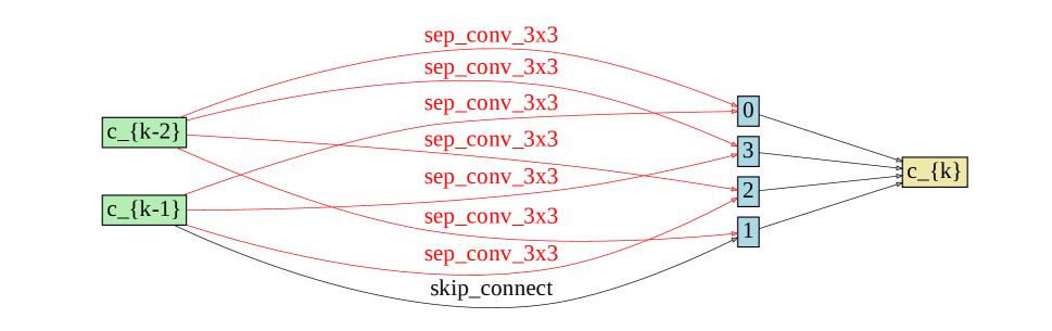
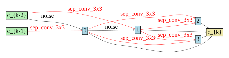
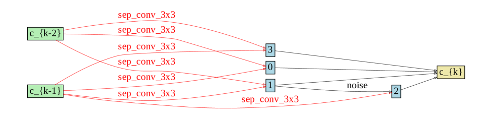
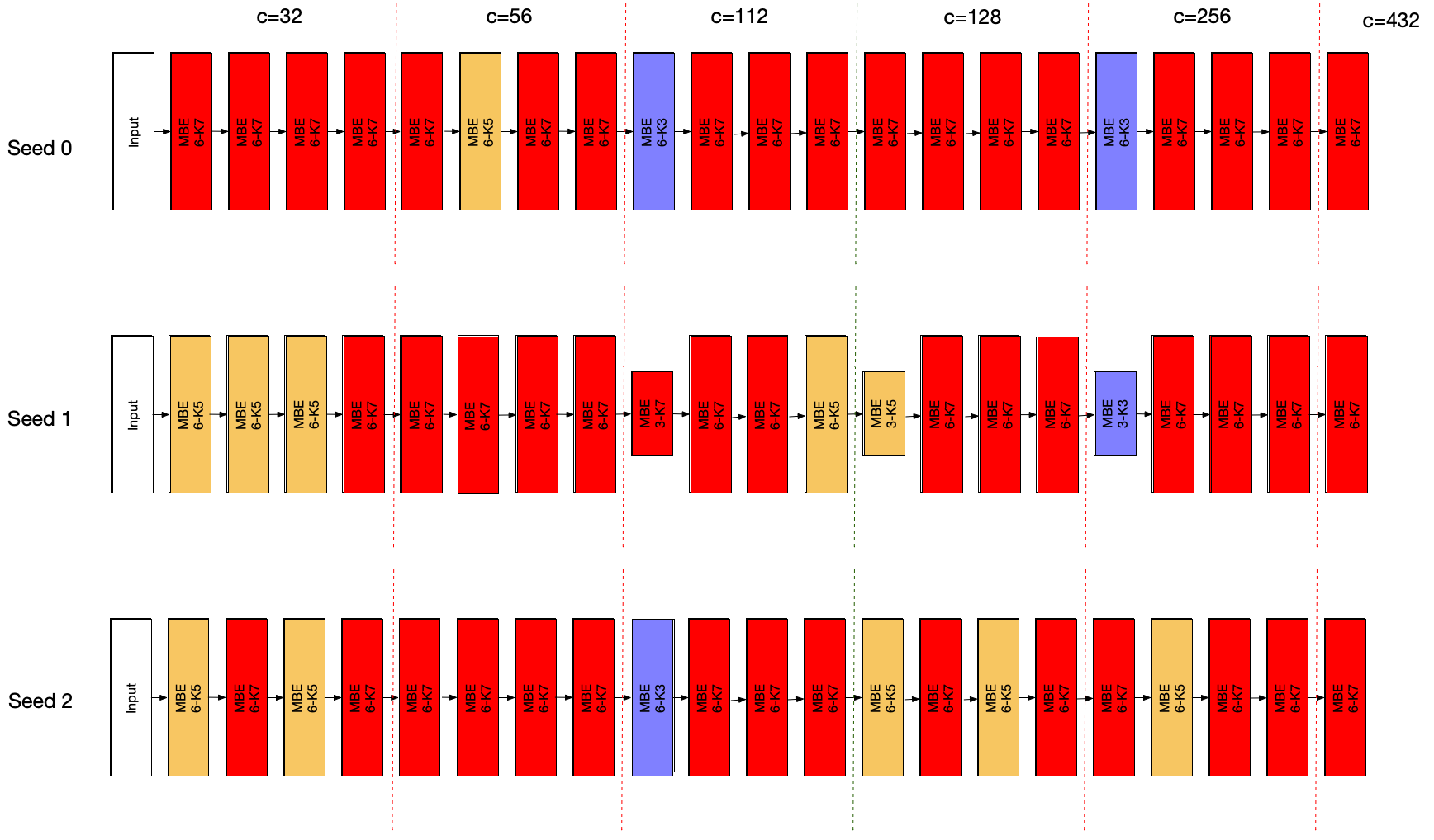
	$edge\backslash op$	none	skip_connect	nor_conv_1x1	nor_conv_3x3	avg_pool_3x3
best-acc	0	94.15	94.18	94.44	94.68	93.86
	1	94.24	94.16	94.49	94.68	94.09
	2	94.25	94.43	94.49	94.68	94.19
	3	94.16	94.68	94.03	94.04	93.85
	4	94.29	94.18	94.56	94.68	94.23
	5	94.05	94.16	94.68	94.56	94.1
avg-acc	0	77.36	81.02	83.81	86.38	87.32
	1	80.03	83.11	85.23	85.99	81.52
	2	82.9	82.44	84.05	84.49	81.98
	3	74.02	85.17	87.3	88.28	81.38
	4	80.14	83.05	85.09	85.7	81.89
	5	77.61	83.43	86.18	86.95	81.74
disc-acc	0	83.27	82.24	65.0	71.76	54.31
	1	84.94	83.23	73.23	76.77	83.45
	2	83.87	83.73	77.33	76.83	83.25
	3	65.77	84.44	75.82	78.68	62.7
	4	83.57	82.03	75.02	76.09	82.56
	5	83.95	82.45	66.69	71.36	80.31
darts-pt1	0	-85.43	-17.02	-78.13	-59.09	-85.34
	1	-85.52	-36.1	-84.39	-80.95	-85.49
	2	-85.51	-80.29	-81.86	-77.68	-85.32
	3	-85.49	-9.86	-81.79	-59.18	-85.48
	4	-85.45	-51.15	-78.84	-64.64	-85.14
	5	-85.54	-32.43	-81.04	-72.75	-85.51
disc-zc	0	3331.01	3445.49	3366.88	3437.55	3423.18
	1	3429.07	3435.75	3407.87	3434.58	3421.44
	2	3428.8	3423.36	3440.93	3437.29	3416.89
	3	3408.99	3464.05	3359.89	3382.18	3431.81
	4	3433.99	3435.57	3424.47	3431.14	3423.15
	5	3434.42	3437.66	3418.57	3397.52	3424.17
zc-pt1	0	-3455.23	-3449.9	-3449.54	-3441.82	-3461.18
	1	-3452.15	-3448.7	-3441.81	-3440.65	-3453.74
	2	-3446.52	-3447.61	-3435.46	-3436.4	-3449.28
	3	-3453.81	-3435.99	-3444.04	-3445.6	-3447.07
	4	-3451.06	-3449.8	-3442.63	-3441.13	-3453.31
	5	-3450.97	-3448.21	-3440.8	-3443.24	-3452.99
darts	0	0.14	0.48	0.13	0.18	0.07
	1	0.12	0.55	0.11	0.12	0.09
	2	0.24	0.33	0.15	0.17	0.11
	3	0.06	0.65	0.08	0.13	0.07
	4	0.12	0.48	0.13	0.17	0.1
	5	0.16	0.49	0.12	0.14	0.09
tenas	0	-38.5	-48.0	-31.0	-6.0	-37.5
	1	-7.0	-55.0	-10.0	-15.0	-39.0
	2	-31.5	-10.0	-30.0	-16.5	-36.5
	3	-34.0	-44.0	-53.5	-23.0	-30.0
	4	-32.0	-32.5	-36.5	-32.0	-52.0
	5	-38.5	-16.0	-20.0	-17.0	-27.5

• Lower is better so we add a negative sign to *-pt scores.

References

- Abdelfattah et al. (2021) Abdelfattah, M. S.; Mehrotra, A.; Dudziak, Ł.; and Lane, N. D. 2021. Zero-Cost Proxies for Lightweight NAS. In International Conference on Learning Representations (ICLR).
- Bellman (1957) Bellman, R. 1957. Dynamic Programming. Dover Publications. ISBN 9780486428093.
- Cai, Zhu, and Han (2019) Cai, H.; Zhu, L.; and Han, S. 2019. ProxylessNAS: Direct Neural Architecture Search on Target Task and Hardware. In International Conference on Learning Representations (ICLR).
- Chen, Gong, and Wang (2021) Chen, W.; Gong, X.; and Wang, Z. 2021. Neural Architecture Search on ImageNet in Four GPU Hours: A Theoretically Inspired Perspective. In International Conference on Learning Representations.
- Chen and Hsieh (2020) Chen, X.; and Hsieh, C.-J. 2020. Stabilizing differentiable architecture search via perturbation-based regularization. In International Conference on Machine Learning (ICML), 1554–1565. PMLR.
- Deng et al. (2009) Deng, J.; Dong, W.; Socher, R.; Li, L.-J.; Li, K.; and Fei-Fei, L. 2009. ImageNet: A Large-Scale Hierarchical Image Database. In Proceedings of the IEEE/CVF Conference on Computer Vision and Pattern Recognition (CVPR).
- Dong and Yang (2020) Dong, X.; and Yang, Y. 2020. NAS-Bench-201: Extending the Scope of Reproducible Neural Architecture Search. In International Conference on Learning Representations (ICLR).
- Dudziak et al. (2020) Dudziak, Ł.; Chau, T.; Abdelfattah, M. S.; Lee, R.; Kim, H.; and Lane, N. D. 2020. BRP-NAS: Prediction-based NAS using GCNs. In Neural Information Processing Systems (NeurIPS).
- Guo et al. (2019) Guo, Z.; Zhang, X.; Mu, H.; Heng, W.; Liu, Z.; Wei, Y.; and Sun, J. 2019. Single Path One-Shot Neural Architecture Search with Uniform Sampling.
- Howard et al. (2019) Howard, A.; Sandler, M.; Chu, G.; Chen, L.-C.; Chen, B.; Tan, M.; Wang, W.; Zhu, Y.; Pang, R.; Vasudevan, V.; Le, Q. V.; and Adam, H. 2019. Searching for MobileNetV3.
- Jacot, Gabriel, and Hongler (2021) Jacot, A.; Gabriel, F.; and Hongler, C. 2021. Neural Tangent Kernel: Convergence and Generalization in Neural Networks (Invited Paper). In Proceedings of the 53rd Annual ACM SIGACT Symposium on Theory of Computing, STOC 2021, 6. New York, NY, USA: Association for Computing Machinery. ISBN 9781450380539.
- Lee, Ajanthan, and Torr (2019) Lee, N.; Ajanthan, T.; and Torr, P. H. 2019. SNIP: Single-shot network pruning based on connection sensitivity. In International Conference on Learning Representations (ICLR).
- Li et al. (2020) Li, G.; Qian, G.; Delgadillo, I. C.; Muller, M.; Thabet, A.; and Ghanem, B. 2020. SGAS: Sequential greedy architecture search. In Proceedings of the IEEE/CVF Conference on Computer Vision and Pattern Recognition (CVPR), 1620–1630.
- Lin et al. (2021) Lin, M.; Wang, P.; Sun, Z.; Chen, H.; Sun, X.; Qian, Q.; Li, H.; and Jin, R. 2021. Zen-NAS: A Zero-Shot NAS for High-Performance Deep Image Recognition. In 2021 IEEE/CVF International Conference on Computer Vision, ICCV 2021.
- Liu, Simonyan, and Yang (2019) Liu, H.; Simonyan, K.; and Yang, Y. 2019. DARTS: Differentiable Architecture Search. In International Conference on Learning Representations (ICLR).
- Luo et al. (2018) Luo, R.; Tian, F.; Qin, T.; Chen, E.; and Liu, T.-Y. 2018. Neural Architecture Optimization. In Proceedings of the 32nd International Conference on Neural Information Processing Systems, NIPS’18, 7827–7838. Red Hook, NY, USA: Curran Associates Inc.
- Mehrotra et al. (2021) Mehrotra, A.; Ramos, A. G.; Bhattacharya, S.; Łukasz Dudziak; Vipperla, R.; Chau, T.; Abdelfattah, M. S.; Ishtiaq, S.; and Lane, N. D. 2021. NAS-Bench-ASR: Reproducible Neural Architecture Search for Speech Recognition. In International Conference on Learning Representations (ICLR).
- Mellor et al. (2021) Mellor, J.; Turner, J.; Storkey, A.; and Crowley, E. J. 2021. Neural Architecture Search without Training. In International Conference on Machine Learning (ICML).
- Pearlmutter (1993) Pearlmutter, B. A. 1993. Fast Exact Multiplication by the Hessian. Neural Computation.
- Pham et al. (2018) Pham, H.; Guan, M.; Zoph, B.; Le, Q.; and Dean, J. 2018. Efficient Neural Architecture Search via Parameters Sharing. In International Conference on Machine Learning (ICML), 4095–4104.
- Real et al. (2019) Real, E.; Aggarwal, A.; Huang, Y.; and Le, Q. V. 2019. Regularized Evolution for Image Classifier Architecture Search. In AAAI Conference on Artificial Intelligence (AAAI).
- Shu, Wang, and Cai (2020) Shu, Y.; Wang, W.; and Cai, S. 2020. Understanding Architectures Learnt by Cell-based Neural Architecture Search. In International Conference on Learning Representations.
- Su et al. (2021) Su, X.; Huang, T.; Li, Y.; You, S.; Wang, F.; Qian, C.; Zhang, C.; and Xu, C. 2021. Prioritized Architecture Sampling with Monto-Carlo Tree Search. In Proceedings of the IEEE/CVF Conference on Computer Vision and Pattern Recognition, 10968–10977.
- Tanaka et al. (2020) Tanaka, H.; Kunin, D.; Yamins, D. L. K.; and Ganguli, S. 2020. Pruning neural networks without any data by iteratively conserving synaptic flow. In Neural Information Processing Systems (NeurIPS).
- Theis et al. (2018) Theis, L.; Korshunova, I.; Tejani, A.; and Huszár, F. 2018. Faster gaze prediction with dense networks and Fisher pruning. ArXiv:1801.05787.
- Turner et al. (2020) Turner, J.; Crowley, E. J.; O’Boyle, M.; Storkey, A.; and Gray, G. 2020. BlockSwap: Fisher-guided Block Substitution for Network Compression on a Budget. In International Conference on Learning Representations (ICLR).
- Wang, Zhang, and Grosse (2020) Wang, C.; Zhang, G.; and Grosse, R. 2020. Picking Winning Tickets Before Training by Preserving Gradient Flow. In International Conference on Learning Representations (ICLR).
- Wang et al. (2021) Wang, R.; Cheng, M.; Chen, X.; Tang, X.; and Hsieh, C.-J. 2021. Rethinking Architecture Selection in Differentiable NAS. In International Conference on Learning Representations (ICLR).
- Wei et al. (2020) Wei, C.; Niu, C.; Tang, Y.; and min Liang, J. 2020. NPENAS: Neural Predictor Guided Evolution for Neural Architecture Search. arXiv:2003.12857.
- Wen et al. (2019) Wen, W.; Liu, H.; Li, H.; Chen, Y.; Bender, G.; and Kindermans, P.-J. 2019. Neural Predictor for Neural Architecture Search. arXiv:1912.00848.
- Wu et al. (2021) Wu, J.; Dai, X.; Chen, D.; Chen, Y.; Liu, M.; Yu, Y.; Wang, Z.; Liu, Z.; Chen, M.; and Yuan, L. 2021. Weak NAS Predictors Are All You Need. arXiv:2102.10490.
- Xu et al. (2020) Xu, Y.; Xie, L.; Zhang, X.; Chen, X.; Qi, G.-J.; Tian, Q.; and Xiong, H. 2020. PC-DARTS: Partial Channel Connections for Memory-Efficient Architecture Search. In International Conference on Learning Representations.
- You et al. (2020) You, S.; Huang, T.; Yang, M.; Wang, F.; Qian, C.; and Zhang, C. 2020. GreedyNAS: Towards Fast One-Shot NAS with Greedy Supernet.
- Yu et al. (2020) Yu, K.; Sciuto, C.; Jaggi, M.; and Claudiu Musat, M. S. 2020. Evaluating The Search Phase of Neural Architecture Search. In International Conference on Learning Representations.
- Zela et al. (2020) Zela, A.; Elsken, T.; Saikia, T.; Marrakchi, Y.; Brox, T.; and Hutter, F. 2020. Understanding and robustifying differentiable architecture search. In International Conference on Learning Representations (ICLR), volume 3, 7.
- Zela, Siems, and Hutter (2020) Zela, A.; Siems, J.; and Hutter, F. 2020. Nas-bench-1shot1: Benchmarking and dissecting one-shot neural architecture search. arXiv preprint arXiv:2001.10422.
- Zhou et al. (2020) Zhou, D.; Zhou, X.; Zhang, W.; Loy, C. C.; Yi, S.; Zhang, X.; and Ouyang, W. 2020. EcoNAS: Finding Proxies for Economical Neural Architecture Search. In Proceedings of the IEEE/CVF Conference on Computer Vision and Pattern Recognition (CVPR).
- Zoph and Le (2017) Zoph, B.; and Le, Q. V. 2017. Neural Architecture Search with Reinforcement Learning. In International Conference on Learning Representations (ICLR).