Joint Client Scheduling and Resource Allocation under Channel Uncertainty in Federated Learning

Abstract

The performance of federated learning (FL) over wireless networks depend on the reliability of the client-server connectivity and clients’ local computation capabilities. In this article we investigate the problem of client scheduling and resource block (RB) allocation to enhance the performance of model training using FL, over a pre-defined training duration under imperfect channel state information (CSI) and limited local computing resources. First, we analytically derive the gap between the training losses of FL with clients scheduling and a centralized training method for a given training duration. Then, we formulate the gap of the training loss minimization over client scheduling and RB allocation as a stochastic optimization problem and solve it using Lyapunov optimization. A Gaussian process regression-based channel prediction method is leveraged to learn and track the wireless channel, in which, the clients’ CSI predictions and computing power are incorporated into the scheduling decision. Using an extensive set of simulations, we validate the robustness of the proposed method under both perfect and imperfect CSI over an array of diverse data distributions. Results show that the proposed method reduces the gap of the training accuracy loss by up to $40.7\,\%$ compared to state-of-the-art client scheduling and RB allocation methods.

I Introduction

The staggering growth of data generated at the edge of wireless networks sparked a huge interest in machine learning (ML) at the network edge, coined edge ML [3]. In edge ML, training data is unevenly distributed over a large number of devices, and every device has a tiny fraction of the data. One of the most popular model training methods in edge ML is federated learning (FL) [4, 5]. The goal of FL is to train a high-quality centralized model in a decentralized manner, based on local model training and client-server communication while training data remains private [4, 6, 3]. Recently, FL over wireless networks gained much attention in communication and networking with applications spanning a wide range of domains and verticals ranging from vehicular communication to ,blockchain and healthcare [6, 5, 7]. The performance of FL highly depends on the communication and link connectivity in addition to the model size and the number of clients engaged in training. The quality of the trained model (inference accuracy) also depends on the training data distributions over devices which generally is non-independent and identically distributed (IID) [8, 9]. Hence, the impact of training data distribution in terms of balanced-unbalancedness and IID versus non-IID ness on model training is analyzed in few works [5, 10, 11]. In [10], the authors have analyzed the effect of non-IID data distribution through numerical simulations for a visual classification task. Likewise in [11], authors have empirically analyzed the impact of non-IID data distribution on the performance of FL.

Except a handful of works [12, 13, 14, 15, 4, 16, 17], the vast majority of the existing literature assumes ideal client-server communication conditions, overlooking channel dynamics and uncertainties. In [12], communication overhead is reduced by using the lazily aggregate gradients (LAG) based on reusing outdated gradient updates. Due to the limitations in communication resources, scheduling the most informative clients is one possible solution [13, 14, 17]. In [13] authors propose a client-scheduling algorithm for FL to maximize the number of scheduled clients assuming that communication and computation delays are less than a predefined threshold but, the impact of client scheduling was not studied. In [14], the authors study the impact of conventional scheduling policies (e.g., random, round robin, and proportional fairness) on the accuracy of FL over wireless networks relying on known channel statistics. In [15], the training loss of FL is minimized by joint power allocation and client scheduling. A probabilistic scheduling framework is proposed in [18], seeking the optimal trade-off between channel quality and importance of model update considering the impact of channel uncertainty in scheduling. Moreover, the impact of dynamic channel conditions on FL is analyzed only in few works [14, 4, 19]. In [4], authors propose over-the-air computation-based approach leveraging the ideas of [20] to speed-up the global model aggregation utilizing the superposition property of a wireless multiple-access channels with scheduling and beamforming. In addition to channel prediction, clients’ computing power are utilized for their local models updates. Stochastic gradient decent (SGD) is widely used for updating their local models, in which the computation is executed sample by sample [21]. In [19], the authors proposed the compressed analog distributed stochastic gradient descent (CA-DSGD) method, which is shown to be robust against imperfect channel state information (CSI) at the devices. While interestingly the communication aspects in FL such as optimal client scheduling and resource allocation in the absence of perfect CSI along with the limitations in processing power for SGD-based local computations are neglected in all these aforementioned works.

Acquiring CSI through pilot sequence exchanges introduces an additional signaling overhead that scales with the number of devices. There are a handful of works dealing with wireless channel uncertainties [22, 23]. Authors in [22] demonstrated the importance of reliable fading prediction for adaptive transmission in wireless communication systems. Channel prediction via fully connected recurrent neural networks are proposed in [23]. Among channel prediction methods, Gaussian process regression (GPR) is a light weight online technique where the objective is to approximate a function with a non-parametric Bayesian approach under the presence of nonlinear and unknown relationships between variables [24, 25]. A Gaussian process (GP) is a stochastic process with a collection of random variables indexed by time or space. Any subset of these random variables forms multidimensional joint Gaussian distributions, in which GP can be completely described by their mean and covariance matrices. motivationgaussianThe foundation of the GPR-approach is Bayesian inference, where a priori model is chosen and updated with observed experimental data [24]. In the literature, GPR is used for a wide array of practical applications including communication systems [26, 27, 28]. In [26] GPR is used to estimate Rayleigh channel. In [27], a problem of localization in a cellular network is investigated with GPR-based possition predictions. In [28], GPR is used to predict the channel quality index (CQI) to reduce CQI signaling overhead. In our prior works, [1, 2], GPR-based channel prediction is used to derive a client scheduling and resource block (RB) allocation policy under imperfect channel conditions assuming unlimited computational power availability per client. Investigating the performance of FL under clients’ limited computation power under both IID and non-IID data distributions remains an unsolved problem.

The main contributions of this work over [1, 2] are the derivation of a joint client scheduling and RB allocation policy for FL under communication and computation power limitations and a comprehensive analysis of the performance of model training as a function of (i) system model parameters, (ii) available computation and communication resources, (iii) non-IID data distribution over the clients in terms of the heterogeneity of dataset sizes and available classes. In this work, we consider a set of clients that communicate with a server over wireless links to train a neural network (NN) model within a predefined training duration. First, we derive an analytical expression for the loss of accuracy in FL with scheduling compared to a centralized training method. In order to reduce the signaling overhead in pilot transmission for channel estimation, we consider the communication scenario with imperfect CSI and we leverage GPR to learn and track the wireless channel while quantifying the information on the unexplored CSI over the network. To do so, we formulate the client scheduling and RB allocation problem as a trade-off between optimal client scheduling, RB allocation, and CSI exploration under both communication and computation resource constraints. noveltypageDue to the stochastic nature of the aforementioned problem, we resort to the dual-plus-penalty (DPP) technique from the Lyapunov optimization framework to recast the problem into a set of linear problems that are solved at each time slot [29]. In this view, we present the joint client scheduling and RB allocation algorithm that simultaneously explore and predict CSI to improve the accuracy of FL over wireless links. With an extensive set of simulations we validate the proposed methods over an array of IID and non-IID data distributions capturing the heterogeneity in dataset sizes and available classes. In addition, we compare the feasibility of the proposed methods in terms of fairness of the trained global model and accuracy. Simulation results show that the proposed method achieves up to $40.7\,\%$ reduction in the loss of accuracy compared to the state-of-the-art client scheduling and RB allocation methods.

The rest of this paper is structured as follows. Section II presents the system model and formulates the problem of model training over wireless links under imperfect CSI. In Section III, the problem is first recast in terms of the loss of accuracy due to client scheduling compared to a centralized training method. Subsequently, GPR-based CSI prediction is proposed followed by the derivation of Lyapunov optimization-based client scheduling and RB allocation policies under both perfect and imperfect CSI. Section IV numerically evaluates the proposed scheduling policies over state-of-the-art client scheduling techniques. Finally, conclusions are drawn in Section V.

II System Model and Problem Formulation

Consider a system consisting of a set $\mathcal{K}$ of $K$ clients that communicate with a parameter server (PS) over wireless links. Therein, the $k$-th client has a private dataset $\mathcal{\mathcal{D}}_{k}$ of size $D_{k}$, which is a partition of the global dataset $\mathcal{\mathcal{D}}$ of size $D=\sum_{k}D_{k}$. For communication with the server for local model updating, a set $\mathcal{B}$ of $B(\leq K$) RBs is shared among those clients.

II-A Scheduling, resource block allocation, and channel estimation

Let $s_{k}(t)\in\{0,1\}$ be an indicator where $s_{k}(t)=1$ indicates that the client $k$ is scheduled by the PS for uplink communication at time $t$ and $s_{k}(t)=0$, otherwise. Multiple clients are simultaneously scheduled by allocating each at most with one RB. Hence, we define the RB allocation vector $\boldsymbol{\lambda}_{k}(t)=[\lambda_{k,b}(t)]_{\forall b\in\mathcal{B}}$ for client $k$ with $\lambda_{k,b}(t)=1$ when RB $b$ is allocated to client $k$ at time $t$, and $\lambda_{k,b}(t)=0$, otherwise. The client scheduling and RB allocation are constrained as follows:

$$s_{k}(t)\leq\mathbf{1}^{\dagger}\boldsymbol{\lambda}_{k}(t)\leq 1\quad\forall k,t,$$ (1)

where $\mathbf{1}^{\dagger}$ is the transpose of the all-one vector. The rate at which the $k$-th client communicates in the uplink with the PS at time $t$ is given by,

$$r_{k}(t)=\textstyle\sum_{b\in\mathcal{B}}\lambda_{k,b}(t)\log_{2}\big{(}1+\frac{p|h_{k,b}(t)|^{2}}{I_{k,b}(t)+N_{0}}\big{)},$$ (2)

where $p$ is a fixed transmit power of client $k$, $h_{k,b}(t)$ is the channel between client $k$ and the PS over RB $b$ at time $t$, $I_{k,b}(t)$ represents the uplink interference on client $k$ imposed by other clients over RB $b$, and $N_{0}$ is the noise power spectral density. Note that, a successful communication between a scheduled client and the server within a channel coherence time is defined by satisfying a target minimum rate. In this regard, a rate constraint is imposed on the RB allocation in terms of a target signal to interference plus noise ratio (SINR) $\gamma_{0}$ as follows:

$$\lambda_{k,b}(t)\leq\mathbb{I}\big{(}\hat{\gamma}_{k,b}(t)\geq\gamma_{0}\big{)}\quad\forall k,b,t,$$ (3)

where $\hat{\gamma}_{k,b}(t)=\frac{p|h_{k,b}(t)|^{2}}{I_{k,b}(t)+N_{0}}$ and the indicator $\mathbb{I}(\hat{\gamma}\geq\gamma_{0})=1$ only if $\hat{\gamma}\geq\gamma_{0}$.

II-B Computational power consumption and computational time

Most of the clients in wireless systems are mobile devices operated by power-limited energy sources, with limited computational capabilities. As demonstrated in [30] the dynamic power consumption $P_{\text{c}}$ of a processor with clock frequency of $\omega$ is proportional to the product of $V^{2}\omega$. Here, $V$ is the supply voltage of the computing, which is approximately linearly proportional to $\omega$ [31]. Motivated by [30] and [31], in this work, we adopt the model $P_{\text{c}}\propto\omega^{3}$ to capture the computational power consumption per client. Due to the concurrent tasks handled by the clients in addition to local model training, the dynamics of the available computing power $P_{\text{c}}$ at a client is modeled as a Poison arrival process [32]. Therefore, we assume that the computing power $P_{\text{c}}^{k}(t)$ of client $k$ at time $t$ follows an independent and identically distributed exponential distribution with mean $\mu_{\text{c}}$. As a result, the minimum computational time required for client $k$ is given by,

$$\tau_{\text{c},{k}}(t)=\frac{\mu_{\text{c}}D_{k}M_{k}}{\sqrt[3]{P_{\text{c}}^{k}(t)}/b},$$ (4)

where $M_{k}$ is the number of SGD iterations computed over $D_{k}$. The constants $\mu_{\text{c}}$ and $b$ are the number of clock cycles required to process a single sample and power utilized per number of computation cycles, respectively. To avoid unnecessary delays in the overall training that are caused by clients’ local computations, we impose a constraint on the computational time, with threshold $\tau_{0}$ over the scheduled clients as follows:

$$s_{k}(t)\leq\mathbb{I}(\tau_{\text{min},{k}}(t)\leq\tau_{0})\quad\forall k,t.$$ (5)

II-C Model training using FL

The goal in FL is to minimize a regularized loss function $F(\boldsymbol{w},\mathcal{\mathcal{D}})=\frac{1}{D}\sum_{\boldsymbol{\boldsymbol{x}}_{i}\in\mathcal{\mathcal{D}}}f(\boldsymbol{\boldsymbol{x}}_{i}^{\dagger}\boldsymbol{w})+\xi\varrho(\boldsymbol{w})$, which is parametrized by a weight vector $\boldsymbol{w}$ (referred as the model) over the global dataset within a predefined communication duration $T$. Here, $f(\cdot)$ captures a loss of either regression or classification task, $\varrho(\cdot)$ is a regularization function such as Tikhonov, $\boldsymbol{\boldsymbol{x}}_{i}$ is the input vector, and $\xi(>0)$ is the regularization coefficient. It is assumed that, clients do not share their data and instead, compute their models over the local datasets.

For distributed model training in FL, clients share their local models that are computed by solving $F(\boldsymbol{w},\mathcal{\mathcal{D}})$ over their local datasets using SGD using the PS, which in return does model averaging and shares the global model with all the clients.

Under imperfect CSI, prior to transmission the channels need to be estimated via sampling. Instead of performing channel measurements beforehand the inferred channels between clients and the PS over each RB are as $\hat{h}(t)=J\big{(}t,\{\tau,h(\tau)\}_{\tau\in\mathcal{N}(t)}\big{)}$ using past $N$ channel observations. channelpredictclaimUnder channel prediction, $h_{k,b}(t)=\hat{h}_{k,b}(t)$ is used as signal to interference plus noise ratio (SINR) in (2) and (3). The choice of small $N$ ensures low computation complexity of the inference task. Here, the set $\mathcal{N}(t)$ consists of $N$ most recent time instances satisfying $s(\tau)=1$ and $\tau<t$. With $\lambda_{k,b}(t)=1$, the channel $h_{k,b}(t)$ is sampled and used as an observation for the future, i.e., the RB allocation and channel sampling are carried out simultaneously. In this regard, we define the information on the channel between client $k$ and the server at time $t$ as $\boldsymbol{j}_{k}(t)=[j_{k,b}(t)]_{b\in\mathcal{B}}$. For accurate CSI predictions, it is essential to acquire as much information about the CSI over the network [33]. This is done by exploring new information by maximizing $\sum_{k}\boldsymbol{j}_{k}^{\dagger}(t)\boldsymbol{\lambda}_{k}(t)$ at each time $t$ while minimizing the loss $F(\boldsymbol{w},\mathcal{\mathcal{D}})$.

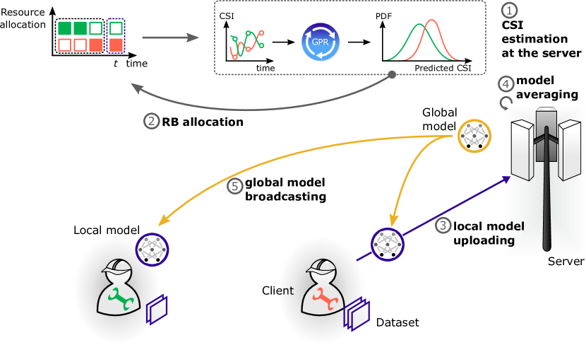
Figure 1: FL with client scheduling under limited wireless resources and imperfect CSI.

Therefore, the empirical loss minimization problem over the training duration is formally defined as follows:

$$\underset{\boldsymbol{w}(t),\boldsymbol{s}(t),\boldsymbol{\Lambda}(t),\forall t}{\text{minimize}} F\big{(}\boldsymbol{w}(T),\mathcal{D}\big{)}-\textstyle\frac{\varphi}{T}\sum_{k,t}\boldsymbol{j}_{k}^{\dagger}(t)\boldsymbol{\lambda}_{k}(t),$$ (6a)

subject to00 $$\eqref{eq:scheduleresource}\text{-}\eqref{eq:allocationindicator},\eqref{computationaltime},$$ (6b)

$$\boldsymbol{A}\boldsymbol{\Lambda}^{\dagger}(t)\preceq\mathbf{1}\quad\forall t,$$ (6c)

$$\mathbf{1}^{\dagger}\boldsymbol{s}(t)\leq B\quad\forall t,$$ (6d)

$$\boldsymbol{s}(t)\in\{0,1\}^{K},\boldsymbol{\lambda}_{k}(t)\in\{0,1\}^{b}\quad\forall t,$$ (6e)

$$\boldsymbol{w}_{k}(t)={\operatorname*{argmin}_{\boldsymbol{w}^{\prime}}F(\boldsymbol{w}^{\prime}|\boldsymbol{w}(t-1),\mathcal{D}_{k}})\quad\forall k,t$$ (6f)

$$\textstyle\boldsymbol{w}(t)=\sum_{k}\frac{D_{k}}{D}s_{k}(t)\boldsymbol{w}_{k}(t)\quad\forall t,$$ (6g)

where $\boldsymbol{\Lambda}^{\dagger}(t)=[\boldsymbol{\lambda}_{k}^{\dagger}(t)]_{k\in\mathcal{K}}$, $\varphi(>0)$ controls the impact of the CSI exploration, and $\boldsymbol{A}$ is a $B\times K$ all-one matrix. The orthogonal channel allocation in (6c) ensures collision-free client uplink transmission with $I_{k,b}(t)=0$ and constraint (6d) defines the maximum allowable clients to be scheduled. The SGD based local model calculation at client $k$ is defined in (6f). gammathresholdThe choice of SINR target $\gamma_{0}$ in (3) ensures that local models are uploaded within a single coherence time interval.

III Optimal client-Scheduling and RB Allocation Policy via Lyapunov Optimization

The optimization problem (6) is coupled over all clients hence, in what follows, we elaborate on the decoupling of (6) over clients and the server, and derive the optimal client scheduling and RB allocation policy.

III-A Decoupling loss function of (6) via dual formulation

Let us consider an ideal unconstrained scenario where the server gathers all the data samples and trains a global model in a centralized manner. Let $F_{0}=\min_{\boldsymbol{w}}F(\boldsymbol{w},\mathcal{D})$ be the minimum loss under centralized training. By the end of the training duration $T$, we define the gap between the proposed FL under communication constraints and centralized training as $\varepsilon(T)=F\big{(}\boldsymbol{w}(T),\mathcal{D}\big{)}-F_{0}$. In other words, $\varepsilon(T)$ is the accuracy loss of FL with scheduling compared to centralized training. Since $F_{0}$ is independent of the optimization variables in (6a), replacing $F(\boldsymbol{w},\mathcal{D})$ by $\varepsilon(T)$ does not affect optimality under the same set of constraints.

theequationTo analyse the loss of FL with scheduling, we consider the dual function of (6a) with the dual variable $\boldsymbol{\theta}=[\theta_{1},\ldots,\theta_{D}]$, $\boldsymbol{X}=[\boldsymbol{X}_{k}]_{k\in\mathcal{K}}$ with $\boldsymbol{X}_{k}=[\boldsymbol{x}_{i}]_{i=1}^{D_{k}}$, and $\boldsymbol{z}=\boldsymbol{X}^{T}\boldsymbol{w}$ as follows:

$$\psi(\boldsymbol{\theta}) =\min_{\boldsymbol{w},\boldsymbol{z}}\Big{(}\textstyle\sum_{\boldsymbol{\boldsymbol{x}}_{i}\in\mathcal{D}}\frac{1}{D}f_{i}(\boldsymbol{\boldsymbol{x}}_{i}^{T}\boldsymbol{w})+\xi\varrho(\boldsymbol{w})+\frac{\boldsymbol{\theta}^{T}(\boldsymbol{z}-\boldsymbol{X}^{T}\boldsymbol{w})}{D}\Big{)}$$ (7a)

$$\textstyle\stackrel{{\scriptstyle a}}{{=}}\frac{1}{D}\underset{\boldsymbol{w}}{\inf}\big{\{}D\xi\varrho(\boldsymbol{w})-\boldsymbol{\theta}^{T}\boldsymbol{X}^{T}\boldsymbol{w}\big{\}}$$

$$\qquad\qquad+\textstyle\sum_{i=1}^{D}\underset{z_{i}}{\inf}\big{\{}-\theta_{i}z_{i}-f_{i}(z_{i})\big{\}}$$ (7b)

$$\stackrel{{\scriptstyle b}}{{=}}\xi\underset{\boldsymbol{w}}{\sup}\big{\{}\boldsymbol{w}^{T}\boldsymbol{v}-\varrho(\boldsymbol{w})\big{\}}+$$

$$\qquad\qquad\textstyle\sum_{k=1}^{K}\sum_{i=1}^{D_{k}}\underset{z_{i}}{\sup}\big{\{}f_{i}(z_{i})+\theta_{i}z_{i}\big{\}}$$ (7c)

$$\textstyle\stackrel{{\scriptstyle c}}{{=}}-\underbrace{\textstyle\sum_{k=1}^{K}\sum_{i=1}^{D_{k}}\frac{1}{D}f_{i}^{*}(-\theta_{i})}_{\#1}-\underbrace{\xi\varrho^{*}(\boldsymbol{v})}_{\#2}.$$ (7d)

Here, step (a) rearranges the terms, (b) converts the infimum operations to supremum while substituting $\boldsymbol{v}={\boldsymbol{X}\boldsymbol{\theta}}/{\xi D}$, and (c) uses the definition of conjugate function $f_{i}^{*}(-\theta_{i})=\textstyle\underset{z_{i}}{\inf}\{-\theta_{i}z_{i}-f_{i}(z_{i})\}$ and $\varrho^{*}(\boldsymbol{v})=\underset{\boldsymbol{w}}{\sup}\{\boldsymbol{w}^{T}\boldsymbol{v}-\varrho(\boldsymbol{w})\}$ [34]. With the dual formulation, the relation between the primal and dual variables is $\boldsymbol{w}=\nabla\varrho^{*}(\boldsymbol{v})$ [14]. Based on the dual formulation, the loss FL with scheduling is $\varepsilon(T)=\psi_{0}-\psi\big{(}\boldsymbol{\theta}(T)\big{)}$ where $\psi_{0}$ is the maximum dual function value obtained from the centralized method.

Note that the first term of (7d) decouples per client and thus, can be computed locally. In contrast, the second term in (7d) cannot be decoupled per client. To compute $\varrho^{*}(\boldsymbol{v})$, first, each client $k$ locally computes $\Delta\boldsymbol{v}_{k}(t)=\frac{1}{\xi D}\boldsymbol{X}_{k}\Delta\boldsymbol{\theta}_{k}(t)$ at time $t$. Here, $\Delta\boldsymbol{\theta}_{k}(t)$ is the change in the dual variable $\boldsymbol{\theta}_{k}(t)$ for client $k$ at time $t$ given as below,

$$\Delta\boldsymbol{\theta}_{k}(t)\approx\textstyle\operatorname*{argmax}_{\boldsymbol{\delta}\in\mathbb{R}^{D_{k}}}\Big{(}-\frac{1}{D}\mathbf{1}^{\dagger}[f_{i}^{*}(-\boldsymbol{\theta}_{k}(t)-\boldsymbol{\delta})]_{i=1}^{D_{k}}\textstyle\\ -\frac{\xi}{K}\varrho^{*}\big{(}\boldsymbol{v}(t)\big{)}\textstyle-\frac{1}{D}\boldsymbol{\delta}^{\dagger}\boldsymbol{X}_{k}\varrho^{*}\big{(}\boldsymbol{v}(t)\big{)}-\frac{\eta/\xi}{2D^{2}}\|\boldsymbol{X}_{k}\boldsymbol{\delta}\|^{2}\Big{)},$$ (8)

where $\eta$ depends on the partitioning of $\mathcal{D}$ [35]. It is worth noting that $\Delta\boldsymbol{\theta}_{k}(t)$ in (8) is computed based on the previous global value $\boldsymbol{v}(t)$ received by the server. Then, the scheduled clients upload $\Delta\boldsymbol{v}_{k}(t)$ to the server. Following the dual formulation, the model aggregation and update in (6g) at the server is modified as follows:

$$\boldsymbol{v}(t+1)\coloneqq\textstyle\boldsymbol{v}(t)+\sum_{k\in\mathcal{K}}s_{k}(t)\Delta\boldsymbol{v}_{k}(t).$$ (9)

Using (9), the server computes the coupled term $\varrho^{*}\big{(}\boldsymbol{v}(t+1)\big{)}$ in (7d).

It is worth noting that from the $t$-th update, $\Delta\boldsymbol{\theta}_{k}(t)$ in (8) maximizes $\Delta\psi\big{(}\boldsymbol{\theta}_{k}(t)\big{)}$, which is the change in the dual function $\psi\big{(}\boldsymbol{\theta}(t)\big{)}$ corresponding to client $k$. Let $\boldsymbol{\theta}^{\star}_{k}(t)$ be the local optimal dual variable at time $t$, in which $\Delta\psi\big{(}\boldsymbol{\theta}^{\star}_{k}(t)\big{)}\geq\Delta\psi\big{(}\boldsymbol{\theta}_{k}(t)\big{)}$ is held. Then for a given accuracy $\beta_{k}(t)\in(0,1)$ of local SGD updates, the following condition is satisfied:

$$\textstyle\frac{\Delta\psi_{k}\big{(}\Delta\boldsymbol{\theta}^{\star}_{k}(t)\big{)}-\Delta\psi_{k}\big{(}\Delta\boldsymbol{\theta}_{k}(t)\big{)}}{\Delta\psi_{k}\big{(}\Delta\boldsymbol{\theta}_{k}(t)\big{)}-\Delta\psi_{k}(0)}\leq\beta_{k}(t),$$ (10)

where $\Delta\psi_{k}(0)$ is the change in $\psi$ with a null update from the $k$-th client. For simplicity, we assume that $\beta_{k,t}=\beta$ for all $k\in\mathcal{K}$ and $t$, hereinafter. With (10), the gap between FL with scheduling and the centralized method is bounded as shown in Theorem 1:

Theorem 1.

The upper bound of $\varepsilon(T)$ after $T$ communication rounds is given by,

$$\varepsilon(T)\leq D\Big{(}1-(1-\beta)\textstyle\operatorname*{\sum\sum}_{t\leq T}^{k\leq K}\frac{D_{k}}{TD}s_{k}(t)\Big{)}^{T}.$$

Proof:

See Appendix -A. ∎

This yields that the minimization of $\varepsilon(T)$ can be achieved by minimizing its upper bound defined in Theorem 1. Henceforth, the equivalent form of (6) is given as follows:

$$\underset{[\Delta\boldsymbol{\theta}_{k}(t)]_{k},\boldsymbol{s}(t),\boldsymbol{\Lambda}(t),\forall t}{\text{minimize}} D\Big{(}1-(1-\beta)\textstyle\sum_{t,k}\frac{D_{k}}{TD}s_{k}(t)\Big{)}^{T}$$

$$\qquad\qquad-\frac{\varphi}{T}\sum_{k,t}\boldsymbol{j}_{k}^{\dagger}(t)\boldsymbol{\lambda}_{k}(t),$$ (11a)

subject to 000 $$\eqref{cns:model_constraints}\text{-}\eqref{cns:boolean},\eqref{eq:delta_theta},\eqref{model_update_new}.$$ (11b)

III-B GPR-based information metric $J(\cdot)$ for unexplored CSI

For CSI prediction, we use GPR with a Gaussian kernel function to estimate the nonlinear relation of $J(\cdot)$ with a GP prior. For a finite data set $\{t_{n},h(t_{n})\}_{n\in\mathcal{N}}$, the aforementioned GP becomes a multi-dimensional Gaussian distribution, with zero mean and covariance $\boldsymbol{C}=[c(t_{m},t_{n})]_{m,n\in\mathcal{N}}$ given by,

$$c(t_{m},t_{n})=\textstyle\exp\Big{(}-\frac{1}{\zeta_{1}}\sin^{2}\big{(}\frac{\pi}{\zeta_{2}}(t_{m}-t_{n})\big{)}\Big{)},$$ (12)

where $\zeta_{1}$ and $\zeta_{2}$ are the length and period hyper-parameters, respectively [36]. Henceforth, the CSI prediction at time $t$ and its uncertainty/variance is given by [37],

$$\hat{h}(t)=c^{\dagger}(t)\boldsymbol{C}^{-1}[h(t_{n})]_{n\in\mathcal{N}},$$ (13)

$$\Upsilon(t)=c(t,t)-c^{\dagger}(t)\boldsymbol{C}^{-1}c(t),$$ (14)

where $c(t)=[c(t,t_{n})]_{n\in\mathcal{N}}$. The client and RB dependence is omitted in the discussion above for notation simplicity. gprmotivation The uncertainty measure $\Upsilon(.)$ of the predicted channel $\hat{h}$ calculated using GPR framework is used as $j(.)$ in (6a) which in turn allowing to exploring and sampling channels with high uncertainty towards improving the prediction accuracy. Finally, it is worth nothing that under perfect CSI $\hat{h}(t)=h(t)$ and $j(t)=0$.

III-C Joint client scheduling and RB allocation

Due to the time average objective in (11a), the problem (11) gives rise to a stochastic optimization problem defined over $t=\{1,\ldots,T\}$. Therefore, we resort to the drift plus penalty (DPP) technique from Lyapunov optimization framework to derive the optimal scheduling policy [29]. Therein, the Lyapunov framework allows us to transform the original stochastic optimization problem into a series of optimizations problems that are solved at each time $t$, as discussed next.

First, we denote $u(t)=(1-\beta)\sum_{k}s_{k}(t)D_{k}/D$ and define its time average $\bar{u}=\sum_{t\leq T}u(t)/T$. Then, we introduce auxiliary variables $\nu(t)$ and $l(t)$ with time average lower bounds $\bar{\nu}\leq\bar{u}$ and $\bar{l}\leq\frac{1}{T}\sum_{k,t}\boldsymbol{j}_{k}^{\dagger}(t)\boldsymbol{\lambda}_{k}(t)\leq l_{0}$, respectively. To track the time average lower bounds, we introduce virtual queues $q(t)$ and $g(t)$ with the following dynamics [29, 38, 39]:

$$q(t+1)=\max\big{(}0,q(t)+\nu(t)-u(t)\big{)},$$ (15a)

$$g(t+1)=\max\big{(}0,g(t)+l(t)-\sum_{k}\boldsymbol{j}_{k}^{\dagger}(t)\boldsymbol{\lambda}_{k}(t)\big{)}.$$ (15b)

Therefore, $\eqref{eq:modified_problem}$ can be recast as follows:

$$\underset{\begin{subarray}{c}[\Delta\boldsymbol{\theta}_{k}(t)]_{k},\boldsymbol{s}(t),\boldsymbol{\Lambda}(t),\nu(t),l(t)\forall t\end{subarray}}{\text{minimize}} D(1-\bar{\nu})^{T}-\varphi\bar{l},$$ (16a)

subject to 00 $$\eqref{cns:all_modified},\eqref{eq:queue},$$ (16b)

$$0\leq\nu(t)\leq 1-\beta\quad\forall t,$$ (16c)

$$0\leq l(t)\leq l_{0}\quad\forall t,$$ (16d)

$$\textstyle u(t)=\sum_{k}\frac{(1-\beta)D_{k}}{D}s_{k}(t)\quad\forall t.$$ (16e)

The quadratic Lyapunov function of $(q(t),g(t))$ is $L(t)={\big{(}q(t)^{2}+g(t)^{2}\big{)}}/{2}$. Given $\big{(}q(t),g(t)\big{)}$, the expected conditional Lyapunov one slot drift at time $t$ is $\Delta L=\mathbb{E}[L(t+1)-L(t)|q(t),g(t)]$. Weighted by a trade-off parameter $\phi(\geq 0)$, we add a penalty term to penalize a deviation from the optimal solution to obtain the Lyapunov DPP [29],

$$\phi\big{(}\frac{\partial}{\partial\nu}[(1-{\nu})^{T}D]_{\nu=\tilde{\nu}(t)}\mathbb{E}[\nu(t)|q(t)]-\varphi\mathbb{E}[l(t)|g(t)]\big{)}=\\ -\phi\Big{(}DT\big{(}1-\tilde{\nu}(t)\big{)}^{T-1}\mathbb{E}[\nu(t)|q(t)]+\varphi\mathbb{E}[l(t)|g(t)]\Big{)},$$ (17)

Here, $\tilde{\nu}(t)=\frac{1}{t}\sum_{\tau=1}^{t}\nu(\tau)$ and $\tilde{l}(t)=\frac{1}{t}\sum_{\tau=1}^{t}l(\tau)$ are the running time averages of the auxiliary variables at time $t$.

Theorem 2.

The upper bound of the Lyapunov DPP is given by,

$$\Delta L-\phi\Big{(}DT\big{(}1-\tilde{\nu}(t)\big{)}^{T-1}\mathbb{E}[\nu(t)|q(t)]+\varphi\mathbb{E}[l(t)|g(t)]\Big{)}\leq\\ \textstyle\mathbb{E}[q(t)\big{(}\nu(t)-u(t)\big{)}+g(t)\big{(}l(t)-\sum_{k}\boldsymbol{j}_{k}^{\dagger}(t)\boldsymbol{\lambda}_{k}(t)\big{)}+L_{0}\\ -\phi\Big{(}DT\big{(}1-\tilde{\nu}(t)\big{)}^{T-1}\nu(t)+\varphi l(t)\Big{)}|q(t),g(t)],$$ (18)

Proof:

See Appendix -B. ∎

The motivation behind deriving the Lyapunov DPP is that minimizing the upper bound of the expected conditional Lyapunov DPP at each iteration $t$ with a predefined $\phi$ yields the tradeoff between the virtual queue stability and the optimality of the solution for (16) [29]. In this regard, the stochastic optimization problem of (16) is solved via minimizing the upper bound in (18) at each time $t$ as follows:

$$\underset{\boldsymbol{s}(t),\boldsymbol{\Lambda}(t),\nu(t),l(t)}{\text{maximize}}\hphantom{0} \textstyle\sum_{k}\big{(}\frac{q(t)(1-\beta)D_{k}}{D}s_{k}(t)+g(t)\boldsymbol{j}_{k}^{\dagger}(t)\boldsymbol{\lambda}_{k}(t)\big{)}-$$

$$\qquad\chi(t)\nu(t)-\big{(}g(t)-\phi\varphi\big{)}l(t),$$ (19a)

subject to $$\eqref{cns:model_constraints}\text{-}\eqref{cns:RB_availability},\eqref{cns:aux_var},\eqref{cns:auxX_var},$$ (19b)

$${\boldsymbol{s}(t)\in\{0,1\}^{K},\boldsymbol{\lambda}_{k}(t)\in\{0,1\}^{b}\quad\forall t},$$ (19c)

where $\chi(t)=q(t)-\phi DT\big{(}1-\tilde{\nu}(t)\big{)}^{T-1}$ and the variables $\Delta\boldsymbol{\theta}_{k}(t)$ with constraints (8) and (9) are decoupled from (19). By relaxing the integer (more specifically, boolean) variables in (19c) as linear variables, the objective and constraints become affine, in which, (19) is recast as a linear program (LP) as follows:

$$\underset{\boldsymbol{s}(t),\boldsymbol{\Lambda}(t),\nu(t),l(t)}{\text{maximize}}\hphantom{0} \textstyle\sum_{k}\big{(}\frac{q(t)(1-\beta)D_{k}}{D}s_{k}(t)+g(t)\boldsymbol{j}_{k}^{\dagger}(t)\boldsymbol{\lambda}_{k}(t)\big{)}-$$

$$\qquad\chi(t)\nu(t)-\big{(}g(t)-\phi\varphi\big{)}l(t),$$ (20a)

subject to $$\eqref{cns:model_constraints}\text{-}\eqref{cns:RB_availability},\eqref{cns:aux_var},\eqref{cns:auxX_var},$$ (20b)

$$\mathbf{0}\preceq\boldsymbol{s}(t),\boldsymbol{\lambda}_{k}(t)\preceq\mathbf{1}.$$ (20c)

Due to the independence, the optimal auxiliary variables are derived by decoupling (16a), (16c), and (16d) as follows:

$$\nu^{\star}(t)=\begin{cases}1-\beta&\text{if}\leavevmode\nobreak\ \chi(t)\geq 0,\\ 0&\text{otherwise},\end{cases}\quad l^{\star}(t)=\begin{cases}l_{0}&\text{if}\leavevmode\nobreak\ g(t)\geq\phi\varphi,\\ 0&\text{otherwise}.\end{cases}$$ (21)

Theorem 3.

theoremipm The optimal scheduling $\boldsymbol{s}^{\star}(t)$ and RB allocation variables $\boldsymbol{\Lambda}^{\star}(t)$ are found using an interior point method (IPM).

Proof:

See Appendix -C. ∎

The joint client scheduling and RB allocation is summarized in Algorithm 1 and the iterative procedure is illustrated in Fig. 2.

Algorithm 1 Joint Client Scheduling and RB Allocation

0:  $\mathcal{D},\gamma_{0},\beta,p,B,\xi$

0:  $\boldsymbol{s}^{\star}(t),\boldsymbol{\Lambda}^{\star}(t)$ for all $t$

1:  $q(0)=g(0)=0$, $\nu(0)=l(0)=0$, $\boldsymbol{v}(0)=\mathbf{0}$

2:  for $t=1$ to $T$ do

3:     Each client update PS with computing power state information (CPSI)

4:     Each client computes $\Delta\boldsymbol{\theta}_{k}(t)$ using (8)

5:     Channel prediction using GPR with (13)

6:     Calculate $\nu^{\star}(t)$ and $l^{\star}(t)$ using (21)

7:     Derive $\boldsymbol{s}^{\star}(t)$ and $\boldsymbol{\Lambda}^{\star}(t)$ by solving (20) using an IPM

8:     Local model state information (MSI) $(\Delta\boldsymbol{v}_{k}(t),\Delta\boldsymbol{\theta}_{k}(t))$ uploading to the server

9:     Update $\tilde{\nu}(t)$, $q(t)$ via (15), $\boldsymbol{v}(t)$ and $\boldsymbol{\theta}(t)$ with (9)

10:     Global model $\boldsymbol{v}(t)$ broadcasting

11:     $t\to t+1$

12:  end for

First, all clients compute their local models using local SGD iterations with available computation power and upload the models to the PS. Parallelly, at the PS, the channels are predicted using GPR based on prior CSI samples and clients are scheduled following the scheduling policy shown in Algorithm 1. Scheduled clients upload their local models to the PS, then at the PS the received models are averaged out to obtain a new global model and broadcast back to all $K$ clients. In this setting, by sampling the scheduled clients, the PS gets additional information on the CSI. In the example presented in Fig. 2, the dashed arrows correspond to non-scheduled clients due to the lack of computational resources and/or poor channel conditions. This strategy allows the proposed scheduling method to avoid unnecessary computation and communication delays.

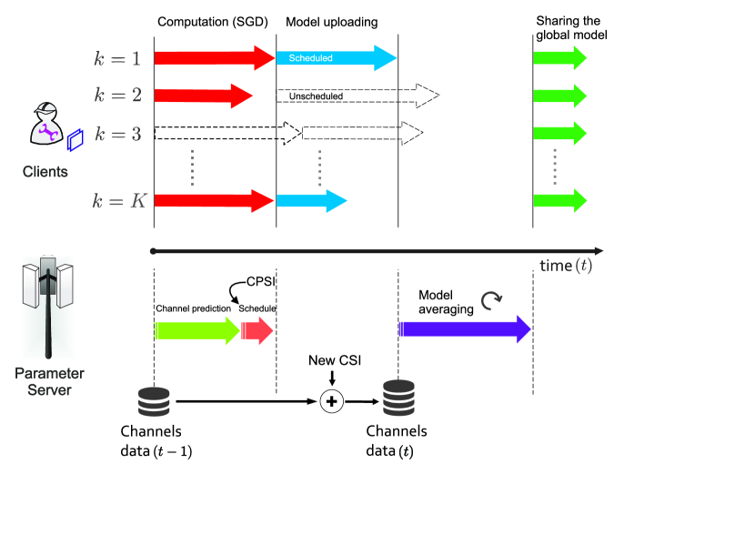
Figure 2: Illustration of the flow of the operation per client and PS over the iterative training process.

III-D Convergence, optimality, and complexity of the proposed solution

WholetextproofConvergenceTowards solving (6a), the main objective (6a) is decoupled over clients and server using a dual formulation. Then, the upper bound of $\varepsilon(T)$, which is the accuracy loss using scheduling compared to a centralized training, is derived in Theorem 1, in which, solving (11) is equivalent to solving (6). It is worth noting that minimizing $\varepsilon(T)$, guarantees convergence to the minimum training loss, which is achieved as $T\to\infty$ [14, Appendix B]. In (11), the minimization of the analytical expression of $\varepsilon(T)$ with a finite $T$ boils down to a stochastic optimization problem with a nonlinear time average objective. The stochastic optimization problem (11) is decoupled into a sequence of optimization problems (19) that are solved at each time iteration $t$ using the Lyapunov DPP technique with guaranteed convergence [40, Section 4]. Following Remark 1, the solution of (20) yields the optimality of (19) ensuring that the convergence guarantees are held under the Lypunov DPP method. proofOptimalitySince the optimal solution of (20) is optimal for (19), the optimality of the proposed solution depends on the recasted problem (16) that relies on the Lypunov DPP technique. Moreover, the optimality of the Lyapunov DPP-based solution is in the order of $\mathcal{O}(\frac{1}{\varphi})$ [40, Section 7.4].

Finally, proofComplexitythe complexity of Algorithm 1 depends on the complexity of the IPM used to solve the LP. Specifically, the complexity of the proposed solution at each iteration is given by the computational complexity of solving the LP which is in the order of $\mathcal{O}(n^{3}L)$ [41] with $n=(D+B+1)K+2$ variables, each of which is represented by a $L$-bits code.

IV Simulation Results

TABLE I: Simulation parameters

Parameter	Value
Number of clients ($K$)	$10$
Number of RB ($B$)	$6$
Local model solving optimality ($\beta$)	$0.7$
Transmit Power (in Watts) ($p$)	$1$
Model training and scheduling
Training duration ($T$)	$100$
Number of local SGD iterations ($M$)	$10$
Learning rate ($\eta$)	$0.2$
Regularizer parameter ($\xi$)	$1$
Lyapunov trade-off parameter ($\phi$)	$1$
Tradeoff weight ($\varphi$)	$1$
SINR threshold ($\gamma_{0}$)	$1.2$
Computation time threshold ($\tau_{0}$)	$1.2$
Channel prediction (GPR)
length parameter ($\zeta_{1}$)	$2$
period parameter ($\zeta_{2}$)	$5$
Number of past observations ($N$)	$20$

In this section, we evaluate the proposed client scheduling method and RB allocation using MNIST and CIFAR-10 datasets assuming $f(\cdot)$ and $\varrho(\cdot)$ as the cross entropy loss function and Tikhonov regularizer, respectively. A subset of the MNIST dataset with 6000 samples consisting of equal sizes of ten classes of 0-9 digits are distributed over $K=10$ clients, whereas for CIFAR-10 data samples are from ten different categories but following the same data distribution. In addition, the wireless channel follows a correlated Rayleigh distribution [42] with mean to noise ratio equal to $\gamma_{0}$. For perfect CSI, a single RB is dedicated for channel estimation. The remaining parameters are presented in Table I.

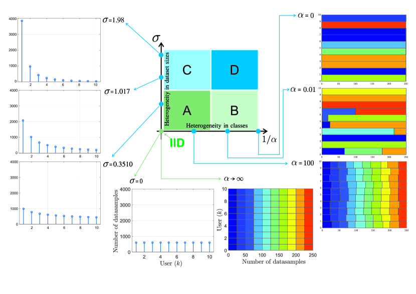
Figure 3: From IID datasets to non-IID datasets under different choices of Zipf parameter $(\sigma)$ and Dirichlet parameter $(\alpha)$. The performance of the proposed algorithms are evaluated under the choices highlighted with the four regions A, B, C, and D.

For IID datasets, training data is partitioned into $K$ subsets of equal sizes with each consisting of equal number of samples from all $10$ classes, which are randomly distributed over the $K$ clients. The impact of the non-IID on the performance is studied for i) heterogeneous dataset sizes: clients having training datasets with different number of samples and ii) heterogeneous class availability: clients’ datasets contain different number of samples per class. The dataset size heterogeneity is modeled by partitioning the training dataset over clients using the Zipf distribution, in which, the dataset of client $k$ is composed of $D_{k}=Dk^{-\sigma}/\sum_{\varkappa\in\mathcal{K}}\varkappa^{-\sigma}$ number of samples [43]. Here, the Zipf’s parameter $\sigma=0$ yields uniform/homogeneous data distribution over clients (600 samples per client), whereas increasing $\sigma$ results in heterogeneous dataset sizes among clients as shown in Fig. 3. To control the heterogeneity in class availability over clients, we adopt the Dirichelet distribution, which is parameterized by a concentration parameter $\alpha\in(0,\infty]$ to distribute data samples from each class among clients [44]. With $\alpha=0$, each client’s dataset consists of samples from a single class in which increasing alpha yields datasets with training data from several classes but the majority of data is from few classes. As $\alpha\to\infty$, each client receives a dataset with samples drawn uniformly from all classes as illustrated in Fig. 3.

Throughout the discussion, centralized training refers to training that takes place at the PS with access to the entire dataset. In addition, how well the global model generalizes for individual clients is termed as “generalization” in this discussion. Training data samples are distributed among clients except in centralized training. In the proposed approach data samples are drawn from ten classes of handwritten digits. We compare several proposed RB allocation and client scheduling policies as well as other baseline methods. Under perfect CSI, two variants of the proposed methods named quantity-aware scheduling QAW and quantity-unaware scheduling QUNAW are compared, whose difference stems from either accounting or neglecting the local dataset size in model updates during scheduling. Under imperfect CSI, GPR-based channel prediction is combined together with QAW yielding the QAW-GPR method. For comparison, we adopt two baselines: a random scheduling technique RANDOM and a proportional fair PF method where fairness is expressed in terms of successful model uploading. In addition, we use the vanilla FL method [6] without RB constraints, denoted as IDEAL hereinafter. All proposed scheduling policies as well as baseline methods are summarized in Table II.

TABLE II: Proposed Algorithms and benchmark algorithm

	Model	Description
{ 91.2 cm[ Proposed Methods ]	QAW-GPR	PS uses dataset sizes to prioritize clients and GPR-based CSI predictions for scheduling.
	QAW	PS uses pilot-based CSI estimation and dataset sizes to prioritize clients.
	QUNAW	PS uses pilot-based CSI estimation without accounting dataset size of clients.
{ 4.21.2 cm[ Baselines ]	RANDOM	Clients are scheduled randomly.
	PF	Clients are scheduled with fairness in terms of successful model uploading.
{ 3.81.2 cm[ Ideal setup ]	IDEAL	All clients are scheduled assuming no communication or computation constraints.

IV-A Loss of accuracy

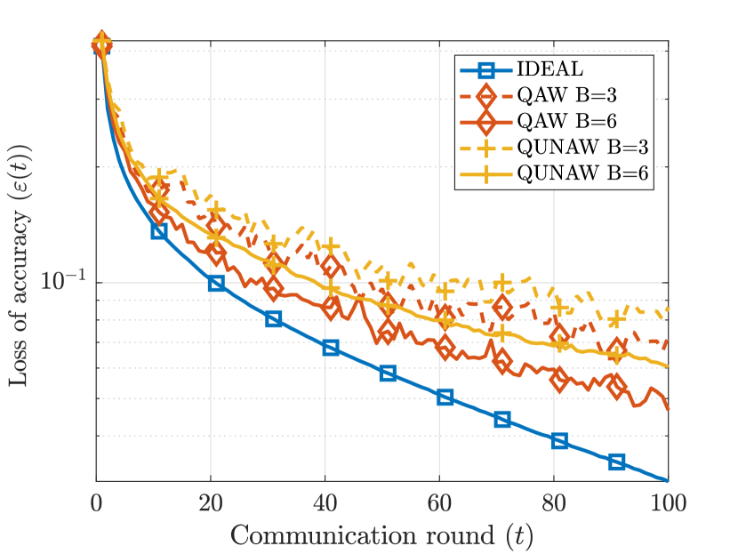
(a) FL with perfect CSI and $B=\{3,6\}$.

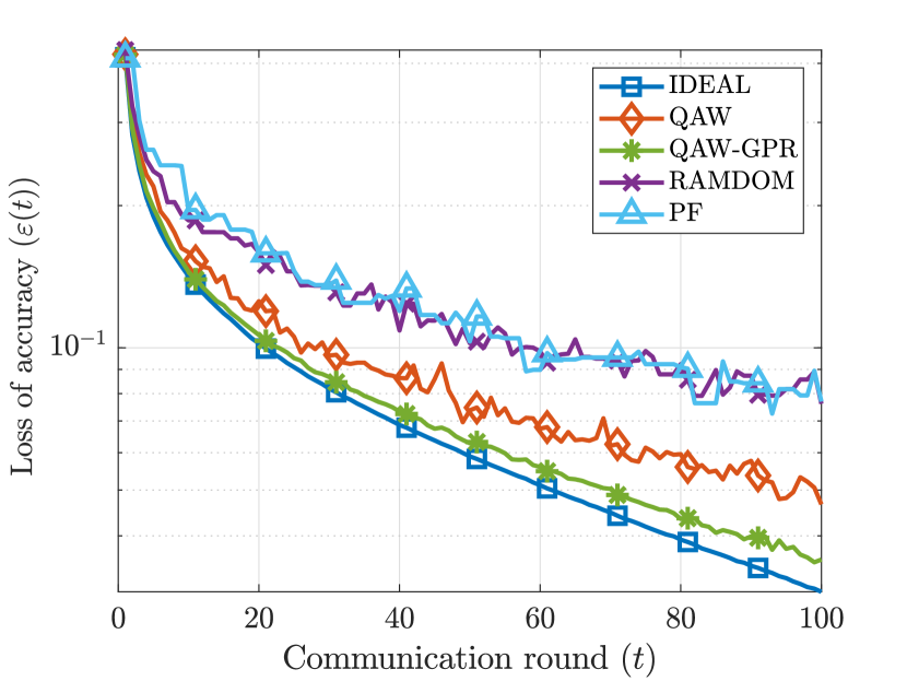
(b) FL with imperfect CSI and $B=6$.

Figure 4: Comparison of the loss of accuracy in all FL methods for each model aggregation round vs. centralized training, Zipf parameter $\sigma=1.017$ and $\alpha\to\infty$(region C of Fig. 3).

Fig. 4 compares the loss of accuracy in all FL methods at each model aggregation round with respect to the centralized model training. Here, we have considered the unbalanced dataset distribution ($\sigma=1.017$) among clients to analyze the impact of dataset size in scheduling. It can be noted that IDEAL has the lowest loss of accuracy $\varepsilon(100)=0.03$ due to the absence of both communication and computation constraints. Under perfect CSI, Fig. 4(a) plots QAW and QUNAW for two different RB values $B\in\{3,6\}$. With a 2$\times$ increase in RB s, the gain of the gap in loss in both QAW and QUNAW is almost the same. For $B=6$, Fig. 4(a) shows that the QAW reduces the gap in loss by $22.8\,\%$ compared to QUNAW. The reason for that is that QAW cleverly schedules clients with higher data samples compared to QUNAW when the dataset distribution among clients is unbalanced. Under imperfect CSI, QAW-GPR, PF, and RANDOM are compared in Fig. 4(b) alongside IDEAL and QAW. While RANDOM and PF show a poor performance, QAW-GPR outperforms QAW by reducing the gap in loss by $23.6\,\%$. The main reason for this improvement is that QAW needs to sacrifice some of its RB s for channel measurements while CSI prediction in QAW-GPR leverages all RB s.

IV-B Impact of system parameters

Fig. 5 shows the impact of the available communication resources (RB s) on the performance of the trained models $F(\boldsymbol{w}(100),\mathcal{\mathcal{D}})$. Without computing and communication constraints, IDEAL shows the lowest loss while RANDOM and PF exhibit the highest losses due to client scheduling with limited RB s. On the other hand the proposed methods QAW-GPR, performs better than QAW and QUNAW for $B\leq 10$ thanks to additional RB s when CSI measurements are missing. Beyond $B=10$, the available number of RB s exceeds $K$, and thus, channel sampling in QAW-GPR is limited to at most $K$ samples. Hence, increasing $B$ beyond $K=10$ results in increased number of under-sampled RB s yielding high uncertainty in GPR and poor CSI predictions. Inaccurate CSI prediction leads to scheduling clients with weak channels (stragglers), which consequently provides a loss of performance in QAW-GPR.

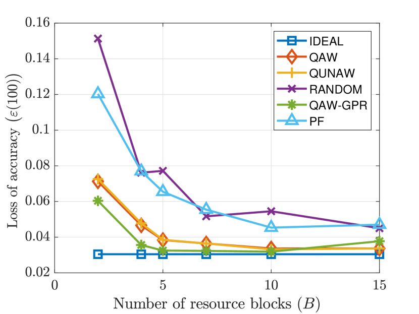
Figure 5: Impact of the available RB s on the gap of loss $\varepsilon(100)$ for $K=10$ clients for $\sigma=0$ and $\alpha\to\infty$ dataset distribution (region A of Fig. 3).

The impact of the number of clients ($K$) in the system with fixed RB s ($B=5$) on the trained models performance and under different training policies is shown in Fig. 6. It can be noted that all methods exhibit higher losses when increasing $K$ due to: i) local training with fewer data samples ($2500/K$) which deteriorates in the non-IID regime, ii) the limited fraction of clients ($5/K$) that are scheduled at once (except for the IDEAL method). The choice of equal number of samples per clients (balanced data sets with $\sigma=0$) results highlights that QAW and QUNAW exhibit identical performance as shown in Fig. 6. Under limited resources, QAW-GPR outperforms all other proposed methods and baselines by reaping the benefits of additional RB s for GPR-based channel prediction. The baseline methods PF and RANDOM are oblivious to both CSI and training performance, giving rise to higher losses compared to the proposed methods.

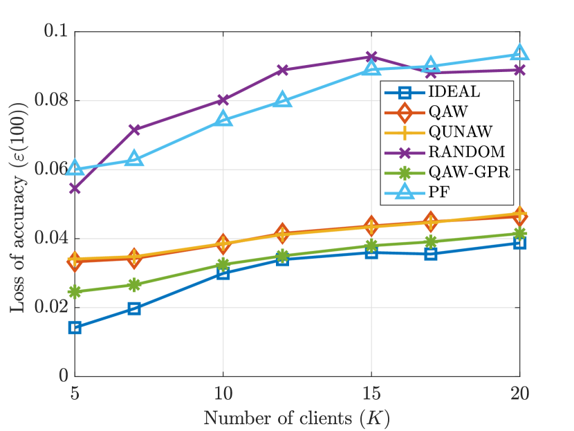
Figure 6: Impact of the number of clients on the gap of accuracy loss $\varepsilon(100)$ for $B=5$ RB s for $\sigma=0$ and $\alpha\to\infty$ dataset distribution (region A of Fig. 3).

Fig. 7 analyzes the performance as the network scales uniformly with the number of RB s and users, i.e., $K=B$. Under ideal conditions, the loss in performance when increasing $K$ shown in Fig. 7 follows the same reasoning presented under Fig. 6. The GPR-based CSI prediction allows QAW-GPR to allocate all RB s for client scheduling yielding the best performance out of the proposed and baseline methods. It is also shown that the worst performance among all methods except IDEAL is at $K=B=2$, owing to the dynamics of CSI leading to scheduling stragglers over limited RB s. With increasing $K$ and $B$, the number of possibilities that clients can be successfully scheduled increases, leading to improved performance in all baseline and proposed methods. In contrast to the baseline methods, the proposed methods optimize client scheduling to reduce the loss of accuracy, achieving closer performance to IDEAL with increasing K and B. However, beyond $K=B=5$, the performance loss due to smaller local datasets outweighs the performance gains coming from an increasing number of scheduled clients, and thus, all three proposed methods follow the trend of IDEAL as illustrated in Fig. 7. Compared to the PF baseline with $K=B=15$, QAW-GPR shows a reduction in the loss of accuracy by $20\,\%$.

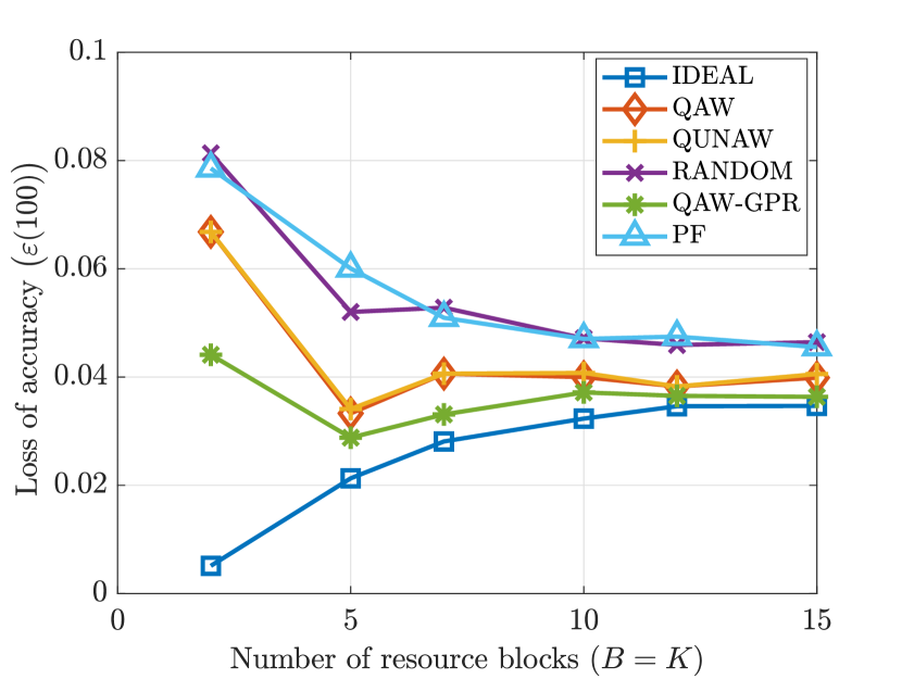
Figure 7: The analysis of the loss of accuracy $\varepsilon(100)$ as the system scales with fixed clients to RB s ratio, (i.e., $B=K$), with $\sigma=0$ and $\alpha\to\infty$ dataset distribution (region A of Fig. 3).

IV-C Impact of dataset distribution

Fig. 8 plots the impact of data distribution in terms of balanced-unbalancedness in terms of training sample size per client on the loss of accuracy $\varepsilon(100)$. Here, the $x$-axis represents the local dataset size of the client having the lowest number of training data, i.e., the dataset size of the 10th client $D_{10}$ as per the Zipf distribution with $\alpha\to\infty$. With balanced datasets, all clients equally contribute to model training, hence scheduling a fraction of the clients results in a significant loss in performance. In contrast, differences in dataset sizes reflect the importance of clients with large datasets. Therefore, scheduling important clients yields lower gaps in performance, even for methods that are oblivious to dataset sizes but fairly schedule all clients, as shown in Fig. 8. Among the proposed methods, QAW-GPR outperforms the others thanks to using additional RB s with the absence of CSI measurement. Compared to the baselines PF and QAW, QAW-GPR shows a reduction of loss of accuracy by $76.3\,\%$, for the highest skewed data distribution ($D_{10}=40$). In contrast, QUNAW yields higher losses compared to QAW, QAW-GPR when training data is unevenly distributed among clients. As an example, the reduction of the loss of accuracy in QAW at $D_{10}=40$ is $25.72\,\%$ compared to $40.7\,\%$ for QUNAW. The reason behind these lower losses is that client scheduling takes into account the training dataset size. For $D_{10}=600$, due to the equal dataset sizes per client, the accuracy loss provided by QAW and QUNAW are identical. Therein, both QAW and QUNAW exhibit about $43.6\,\%$ reduction in accuracy loss compared to RANDOM.

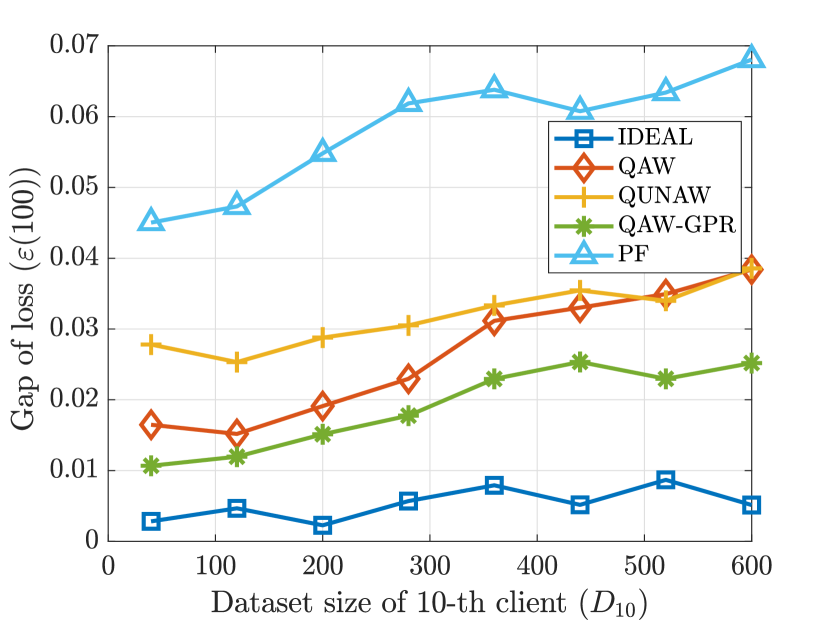
Figure 8: Impact of dataset distribution balanced-unbalancedness on the loss of accuracy $\varepsilon(100)$ for $B=5$, $K=10$, with $\alpha\to\infty$.

Next in Fig. 9, we analyze the impact of non-IID data in terms of the available number of training data from all classes on the accuracy of the trained model. Here, we compare the performance of the proposed methods with the baselines for several choices of $\alpha$ with $D_{k}=250$ for all $k\in\mathcal{K}$ (i.e., $\sigma=0$). Fig. 3 shows the class distribution over clients for different choices of $\alpha$ with equal dataset size $D_{k}=250$. Fig. 9 illustrates that the training performance degrades as the samples data distribution becomes class wise heterogeneous. For instance from the IID case ($\alpha=0$) to the case with $\alpha\to\infty$ case, QAW achieves a loss of accuracy reduction by $86.5\,\%$ compared to $\alpha=0$. However, QAW, QAW-GPR and QUNAW perform better than RANDOM and PF. Finally, it can be noticed that from $\alpha=0.01$ to $\alpha=10$ the gap in terms of accuracy loss performance of the trained model increases rapidly for all methods. Beyond those points, changes are small comparably to the inner points.

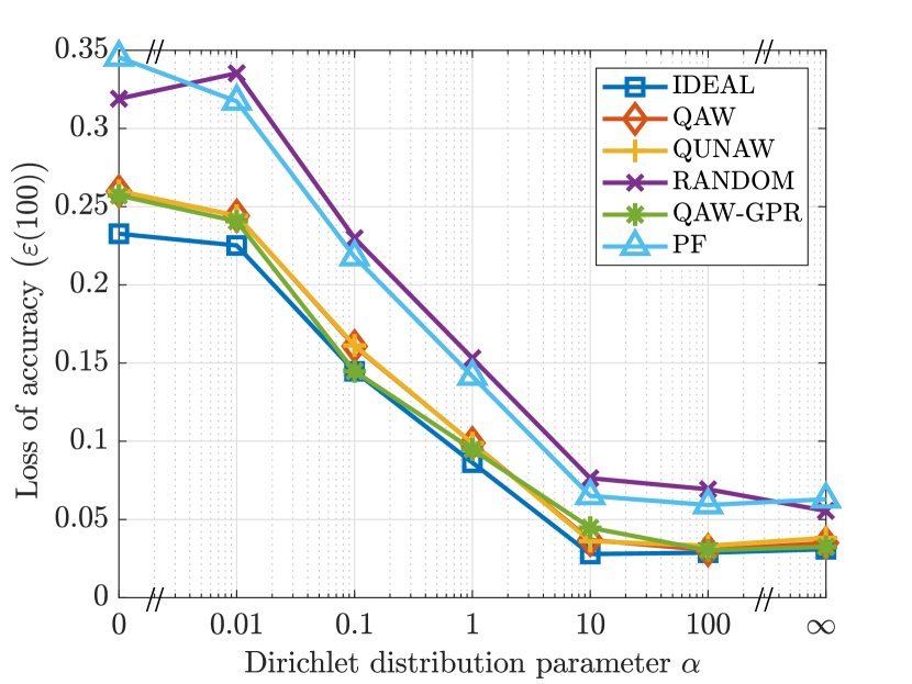
Figure 9: Impact of the class-wise data heterogeneity on the loss of accuracy with $\sigma=0$.

IV-D Impact of computing resources

The impact of the limitations in computation resources in model training and client scheduling is analyzed in Fig. 10. Since allocating RB s to stragglers results in poor RB utilization, we define the RB utilization metric as the percentage of RB s used for a successful model upload over the allocated RB s. Then we compare two variants of QAW with and without considering the computation constraint (5) referred to as CAW (original QAW in the previous discussions) and CUAW, respectively. It is worth highlighting that the computation threshold is inversely proportional to the average computing power availability as per (4), i.e. lower $\tau_{0}$ corresponds to higher $\varepsilon(t)$ and vice versa. Fig. 10 indicates that the use of CPSI for client scheduling in CAW reduces the number of scheduled computation stragglers resulting in a lower accuracy loss, in addition to higher RB utilization over CUAW. Overall, CAW with QAW scheduling performs better than CUAW with QAW scheduling. For instance, compared to CUAW, CAW achieves $11.6\,\%$ reduction in loss of accuracy with $\tau_{0}=0.6$ which increases to $43.1\,\%$ with $\tau_{0}=1.4$. When $\tau_{0}$ is small, the number of stragglers increases leading to poor performance for both CAW and CUAW. It is worth nothing that considering CPSI in the scheduling, CAW achieves at least $18.2\,\%$ increase in RB utilization in addition to the loss of accuracy reduction by at least $11.6\,\%$.

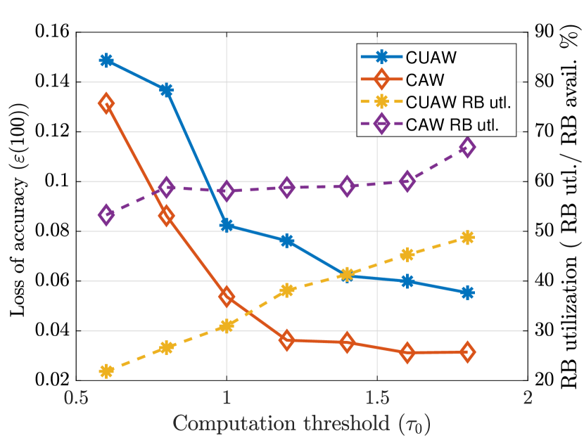
Figure 10: Impact of CPSI for QAW scheduling

The impact of local SGD iterations under limited computing power availability is analyzed in Fig. 11. Due to the assumption of unlimited computing power availability, IDEAL performs well with the increasing local SGD iterations. Similarly, gradual reductions in the loss of accuracy for both QAW and PF can be seen as $M$ increases from two to eight. However, further increasing $M$ results in longer delays for some clients in local computing under limited processing power as per (4). Such computation stragglers do not contribute to the training in both PF (drops out due to the computation constraint) and QAW (not scheduled). Hence, increasing local SGD iterations beyond $M=8$ results in fewer clients to contribute for the training, in which, increased losses of accuracy with QAW and PF are observed as shown in Fig. 11.

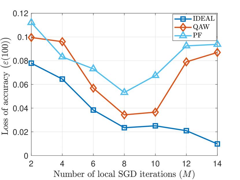
Figure 11: Impact of number of local SGD iterations for loss of accuracy $\varepsilon(100)$

IV-E Fairness

Fig.12 indicates how well the global model generalizes for individual clients. Therein, the global model is used at the client side for inference, and the per client histogram of model accuracy is presented. It can be seen that, the global model in IDEAL generalizes well over the clients yielding the highest accuracy on average $(96.8\,\%)$ over all clients and the lowest variance with $5.6$. With QAW-GPR, $96.1\,\%$ average accuracy and variance of $7.8$ is observed. It is also seen that QAW and QUNAW have almost equal means ($95.2\,\%$) and variances of $15.2$ and $16.3$, respectively. Scheduling clients with a larger dataset in QAW provides a lower variance in accuracy compared to QUNAW. Although RANDOM and PF are CSI-agnostic, they yield an average accuracy of $93.4\,\%$ and $94.1\,\%$ respectively with the highest variance of $18.2$ and $17.6$. This indicates that client scheduling without any insight on datasize distribution and CSI fails to provide high training accuracy or fairness under communication constraints.

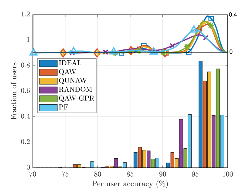
Figure 12: Fairness comparison of the training accuracy among clients, Zipf parameter $\sigma=1.071$ and $\alpha\to\infty$ (region C of Fig. 3).

Finally, Fig. 13 compares the generalization performance of one of the proposed methods, QAW, for CIFAR-10 dataset instead of MNIST under both IID and non-IID data. In contrast to MNIST, CIFAR-10 consists of color images of physical objects from ten distinct classes [45]. For training, we adopt a 3-layer convolutional neural network (CNN) with $K=10$ clients training over $T=1000$ iterations. A total of $2500$ data samples are distributed over the clients under four settings corresponding to the four regions in Fig. 3: i) IID data with $\alpha\to\infty$ and $\sigma=0$ in region A, ii) equal dataset sizes $(\alpha=0)$ under heterogeneous class availability $(\alpha=0)$ in region B, iii) homogeneous class availability $(\alpha\to\infty)$ with heterogeneous dataset sizes $(\sigma=1.017)$ in region C, and iv) heterogeneity in both $(\sigma=1.017)$ and $(\alpha=0)$ under region D. Fig. 13(a) indicates that the training performance with CIFAR-10 dataset significantly suffers from non-IID data under IDEAL communication and computation conditions. Interestingly, the proposed QAW yields identical performance than IDEAL under balanced datasets disregarding the identicalness of the data. However, with unbalanced datasets, the training performance of QAW is degraded as illustrated in Fig. 13(b). The underlying reason is that the unbalanced datasets induce non-IID data at each client, and scheduling fewer clients is insufficient to obtain higher training performance.

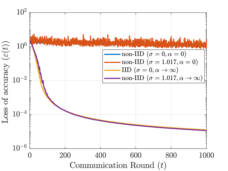
(a) IDEAL scheduling

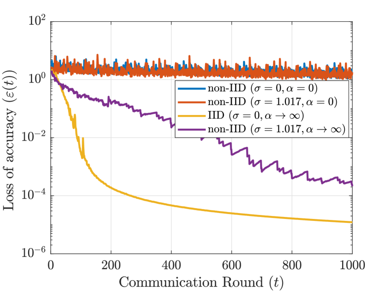
(b) QAW scheduling

Figure 13: Performance comparison of the proposed QAW scheduling approach on CIFAR-10 trained with CNN vs. the IDEAL scheduling scheme.

V Conclusion

In this work, FL over wireless networks with limited computational and communication resources, and under imperfect CSI is investigated. To achieve a training performance close to a centralized training setting, a novel client scheduling and RB allocation policy leveraging GPR-based channel prediction is proposed. Through extensive sets of simulations the benefits of FL using the proposed client scheduling and RB allocation policy are validated and analyzed in terms of (i) system parameters, model performance and computation resource limitations (number of RB s, number of clients) and (ii) heterogeneity of data distribution over clients (balanced-unbalanced, IID and non-IID). Results show that the proposed methods reduce the gap of the accuracy by up to $40.7\,\%$ compared to state-of-the-art client scheduling and RB allocation methods.

-A Proof of Theorem 1

After $t$ and $t+1$ communication rounds, the expected increment in the dual function of (6a) is,

$$\mathbb{E}[\psi(\boldsymbol{\theta}(t+1))-\psi(\boldsymbol{\theta}(t))] \geq\mathbb{E}[\psi(\boldsymbol{\theta}(t+1))]-\mathbb{E}[\psi(\boldsymbol{\theta}(t))].$$

This inequality holds since the expectations of difference is greater than the difference of the expectations of a convex function. By adding and subtracting the optimal dual function value to the R.H.S. :

$$\mathbb{E}[\psi(\boldsymbol{\theta}(t+1))-\psi(\boldsymbol{\theta}(t))]\geq\mathbb{E}[\psi(\boldsymbol{\theta}^{\star})]-\mathbb{E}[\psi(\boldsymbol{\theta}(t))]\\ \qquad\qquad\qquad\qquad\qquad\qquad\qquad+\mathbb{E}[\psi(\boldsymbol{\theta}(t+1))]-\mathbb{E}[\psi(\boldsymbol{\theta}^{\star})]\\ =\textstyle\sum_{k=1}^{K}\Delta\psi(\Delta\boldsymbol{\theta}_{k}^{\star}(t))-\mathbb{E}[\psi(\boldsymbol{\theta}(t))]+\textstyle\sum_{k=1}^{K}\Delta\psi(\Delta\boldsymbol{\theta}_{k}(t))\\ -\textstyle\sum_{k=1}^{K}\Delta\psi(\Delta\boldsymbol{\theta}_{k}^{\star}(t)).$$ (22)

From (10) and following definition $\mathbb{E}[\psi(\boldsymbol{\theta}(t))]=\textstyle\sum_{i=0}^{K}\Delta\psi(0)$,

$$\quad\mathbb{E}[\psi(\boldsymbol{\theta}(t+1))-\psi(\boldsymbol{\theta}(t))]$$

$$\geq\textstyle\sum_{k=1}^{K}\Delta\psi(\Delta\boldsymbol{\theta}_{k}^{\star}(t))-\mathbb{E}[\psi(\boldsymbol{\theta}(t))]$$

$$\hskip 85.35826pt-\beta\big{\{}\textstyle\sum_{k=1}^{K}\Delta\psi(\Delta\boldsymbol{\theta}_{k}^{\star}(t))-\mathbb{E}[\psi(\boldsymbol{\theta}(t))]\big{\}}$$

$$=(1-\beta)\big{\{}\textstyle\sum_{k=1}^{K}\Delta\psi(\Delta\boldsymbol{\theta}_{k}^{\star}(t))-\mathbb{E}[\psi(\boldsymbol{\theta}(t))]\big{\}}.$$

However by selecting subset of users per iteration and repeating up to only $t$ number of communication iterations the bound is lower bounded as below,

$$\mathbb{E}[\psi(\boldsymbol{\theta}(t+1))-\psi(\boldsymbol{\theta}(t))]$$

$$\geq(1-\beta)\big{\{}\textstyle\sum_{k=1}^{K}\Delta\psi(\Delta\boldsymbol{\theta}_{k}^{\star}(t))-\mathbb{E}[\psi(\boldsymbol{\theta}(t))]\big{\}}$$

$$\geq(1-\beta)\big{(}\textstyle\sum_{\tau=1}^{t}\textstyle\sum_{i=1}^{K}\frac{D_{k}}{tD}s_{k}(t)\big{)}\big{\{}\sum_{k=1}^{K}\Delta\psi(\Delta\boldsymbol{\theta}_{k}^{\star}(t))$$

$$\hskip 182.09746pt-\mathbb{E}[\psi(\boldsymbol{\theta}(t))]\big{\}}$$

Now, following [14, Appendix B], $\{\sum_{k=1}^{K}\Delta\psi(\Delta\boldsymbol{\theta}_{k}^{\star}(t))-\mathbb{E}[\psi(\boldsymbol{\theta}(t))]\}\geq\bar{s}\big{\{}\psi(\boldsymbol{\theta}^{\star})-\mathbb{E}[\psi(\boldsymbol{\theta}(t))]\big{\}}$, where $\bar{s}\in(0,1)$, we can have,

$$\varepsilon(T) =\mathbb{E}[\psi(\boldsymbol{\theta}^{\star})-\psi(\boldsymbol{\theta}(T+1))]$$

$$=\mathbb{E}[\psi(\boldsymbol{\theta}^{\star})-\psi(\boldsymbol{\theta}(T))]-\mathbb{E}[\psi(\boldsymbol{\theta}(T+1))-\psi(\boldsymbol{\theta}(T))]$$

$$\leq\mathbb{E}[\psi(\boldsymbol{\theta}^{\star})-\psi(\boldsymbol{\theta}(T))]-$$

$$\quad(1-\beta)\big{(}\textstyle\sum_{\tau=1}^{t}\sum_{i=1}^{K}\frac{D_{k}}{TD}s_{k}(t)\big{)}\big{\{}\psi(\boldsymbol{\theta}^{\star})-\mathbb{E}[\psi(\boldsymbol{\theta}(T))]\big{\}}$$

$$=\big{(}1-(1-\beta)\textstyle\sum_{\tau=1}^{T}\sum_{i=1}^{K}\frac{D_{k}}{TD}s_{k}(t)\big{)}\big{\{}\psi(\boldsymbol{\theta}^{\star})$$

$$\hskip 170.71652pt-\mathbb{E}[\psi(\boldsymbol{\theta}(T))]\big{\}}$$

$$\leq\big{(}1-(1-\beta)\textstyle\sum_{\tau=1}^{T}\sum_{i=1}^{K}\frac{D_{k}}{TD}s_{k}(t)\big{)}^{T}\big{\{}\psi(\boldsymbol{\theta}^{\star})$$

$$\hskip 170.71652pt-\mathbb{E}[\psi(\boldsymbol{\theta}(0))]\big{\}}$$

In [46], it is proved that $\big{\{}\psi(\boldsymbol{\theta}^{\star})-\mathbb{E}[\psi(\boldsymbol{\theta}(0))]\big{\}}<D$. Following that,

$$\varepsilon(T) \leq\bigg{(}1-(1-\beta)\sum_{\tau=1}^{T}\sum_{i=1}^{K}\frac{D_{k}}{TD}s_{k}(t)\bigg{)}^{T}D.$$

-B Proof of Theorem 2

Using the inequality $\max(0,x)^{2}\leq x^{2}$, on (15) we have,

$$\frac{q^{2}(t+1)}{2}\leq\frac{q^{2}(t)}{2}+\frac{\big{(}\nu(t)-u(t)\big{)}^{2}}{2}+q(t)\big{(}\nu(t)-u(t)\big{)},$$ (23a)

$$\frac{g^{2}(t+1)}{2}\leq\frac{g^{2}(t)}{2}+\frac{\big{(}l(t)-\sum_{k}\boldsymbol{j}_{k}^{\dagger}(t)\boldsymbol{\lambda}_{k}(t)\big{)}^{2}}{2}+g(t)\big{(}l(t)$$

$$-\textstyle\sum_{k}\boldsymbol{j}_{k}^{\dagger}(t)\boldsymbol{\lambda}_{k}(t)\big{)}.$$ (23b)

With $L(t)={\big{(}q(t)^{2}+g(t)^{2}\big{)}}/{2}$, one slot drift $\Delta L$ can be expressed as follows:

$$\Delta L\leq\mathbb{E}[q(t)\big{(}\nu(t)-u(t)\big{)}+g(t)\big{(}l(t)-\sum_{k}\boldsymbol{j}_{k}^{\dagger}(t)\boldsymbol{\lambda}_{k}(t)\big{)}\\ +\big{(}\nu(t)-u(t)\big{)}^{2}/2+\big{(}l(t)-\textstyle\sum_{k}\boldsymbol{j}_{k}^{\dagger}(t)\boldsymbol{\lambda}_{k}(t)\big{)}^{2}/2|q(t),g(t)].$$ (24)

$L_{0}$ is a uniform bound on $\big{(}\nu(t)-u(t)\big{)}^{2}/2+\big{(}l(t)-\sum_{k}\boldsymbol{j}_{k}^{\dagger}(t)\boldsymbol{\lambda}_{k}(t)\big{)}^{2}/2$ for all $t$, thus (24) can be expressed as follows:

$$\Delta L\leq\mathbb{E}[q(t)\big{(}\nu(t)-u(t)\big{)}+g(t)\big{(}l(t)-\textstyle\sum_{k}\boldsymbol{j}_{k}^{\dagger}(t)\boldsymbol{\lambda}_{k}(t)\big{)}+\\ \hskip 142.26378ptL_{0}|q(t),g(t)].$$ (25)

Adding penalty term (17), upper bound of DPP can be expressed as,

$$\Delta L-\phi\Big{(}DT\big{(}1-\tilde{\nu}(t)\big{)}^{T-1}\mathbb{E}[\nu(t)|q(t)]+\varphi\mathbb{E}[l(t)|g(t)]\Big{)}\leq\\ \textstyle\mathbb{E}[q(t)\big{(}\nu(t)-u(t)\big{)}+g(t)\big{(}l(t)-\sum_{k}\boldsymbol{j}_{k}^{\dagger}(t)\boldsymbol{\lambda}_{k}(t)\big{)}+L_{0}\\ -\phi\Big{(}DT\big{(}1-\tilde{\nu}(t)\big{)}^{T-1}\nu(t)+\varphi l(t)\Big{)}|q(t),g(t)],$$ (26)

-C Proof of Theorem 3

proofipm Let $\Theta_{k}=\frac{q(t)(1-\beta)D_{k}}{D}$, $\Omega_{k,b}=g(t)j_{k,b}(t)$, and $\mathcal{B}^{\prime}$ and $\mathcal{K}^{\prime}$ be the sets of allocated resource blocks and scheduled clients respectively.

Consider a scenario with non-integer solutions at optimality, i.e., $\lambda^{\star}_{k,b}\in(0,1]$ for $b\in\mathcal{B}^{\prime}$ and $s^{\star}_{k}\in(0,1]$ for $k\in\mathcal{K}^{\prime}$. Note that for all $b\in\mathcal{B}^{\prime}$, $\Omega_{k,b}=\Phi$ for some $\Phi(\geq 0)$ is held ($\because$ if $\Omega_{k,b^{\prime}}>\Phi$ for some $b^{\prime}\in\mathcal{B}^{\prime}$, then optimality holds only when $\lambda_{k,b^{\prime}}=1$ and $\lambda_{k,b}=0$ for all $b\notin\mathcal{B}^{\prime}\setminus\{b^{\prime}\}$). Moreover, optimality satisfies $\mathbf{1}^{\dagger}\boldsymbol{\lambda}_{k}=1$. With the constraint (1), this yields $\sum_{b\in\mathcal{B}}\Omega_{k,b}\lambda_{k,b}=\sum_{b\in\mathcal{B^{\prime}}}\Phi\lambda_{k,b}=\Phi$. Hence, assigning $\lambda_{k,b^{\prime}}=1$ for any $b^{\prime}\in\mathcal{B}^{\prime}$ with $\lambda_{k,b^{\prime\prime}}=0$ for all $b^{\prime\prime}\notin\mathcal{B}^{\prime}\setminus\{b^{\prime}\}$ satisfies all constraints while resulting in the same optimal value, i.e., $\mathbf{1}^{\dagger}\boldsymbol{\lambda}_{k}=\Phi$. Hence, it can be noted that a solution with non-integer $\boldsymbol{\lambda}_{k}^{\star}$ is not unique and there exists a corresponding integer solution for $\boldsymbol{\lambda}_{k}^{\star}$ [claim A].

Substituting the above result in (1) yields $s_{k}\leq 1$ and hence, (1) and (20c) overlap. Following the same argument as for $\boldsymbol{\lambda}_{k}^{\star}$, it can be shown that there exists an integer solution for $s_{k}^{\star}$ that yields the same optimal value as with $s_{k}^{\star}\in(0,1]$ for $k\in\mathcal{K}^{\prime}$ [claim B].

Based on the claims A and B, it can be noted that any non-integer optimal solution is not unique, and there exists at least one integer solution for $\boldsymbol{S}^{\star}$ and $\boldsymbol{\Lambda}^{\star}$. Hence, by solving (20) using IPM and then selecting integer values for $\boldsymbol{S}^{\star}$ and $\boldsymbol{\Lambda}^{\star}$, the optimal solution of (19) is obtained.

Madhusanka Manimel Wadu received his B.Sc. (Hons) degree in Electrical and Electronics Engineering from the University of Peradeniya, Sri Lanka, in 2015 and M.Sc. degree in wireless communication engineering from the University of Oulu, Finland by the end of 2019. He was a research assistant (part-time) at the University of Oulu, Finland from 2018 to 2019 and he has almost three years of industry exposure in Sri Lanka. He is currently a Ph.D. student at the University of Oulu, Finland. His research interests include artificial intelligence (AI), machine learning improvements in the perspective of communication, and wireless channel predictions.

Sumudu Samarakoon (S’08, M’18) received the B.Sc. degree (honors) in electronic and telecommunication engineering from the University of Moratuwa, Moratuwa, Sri Lanka, in 2009, the M.Eng. degree from the Asian Institute of Technology, Khlong Nueng, Thailand, in 2011, and the Ph.D. degree in communication engineering from the University of Oulu, Oulu, Finland, in 2017. He is currently a Docent (Adjunct Professor) with the Centre for Wireless Communications, University of Oulu. His main research interests are in heterogeneous networks, small cells, radio resource management, machine learning at wireless edge, and game theory. Dr. Samarakoon received the Best Paper Award at the European Wireless Conference, Excellence Awards for innovators and the outstanding doctoral student in the Radio Technology Unit, CWC, University of Oulu, in 2016. He is also a Guest Editor of Telecom (MDPI) special issue on “millimeter wave communications and networking in 5G and beyond.”

Dr Mehdi Bennis is an Associate Professor at the Centre for Wireless Communications, University of Oulu, Finland, Academy of Finland Research Fellow and head of the intelligent connectivity and networks/systems group (ICON). His main research interests are in radio resource management, heterogeneous networks, game theory and distributed machine learning in 5G networks and beyond. He has published more than 200 research papers in international conferences, journals and book chapters. He has been the recipient of several prestigious awards including the 2015 Fred W. Ellersick Prize from the IEEE Communications Society, the 2016 Best Tutorial Prize from the IEEE Communications Society, the 2017 EURASIP Best paper Award for the Journal of Wireless Communications and Networks, the all-University of Oulu award for research, the 2019 IEEE ComSoc Radio Communications Committee Early Achievement Award and the 2020 Clarviate Highly Cited Researcher by the Web of Science. Dr Bennis is an editor of IEEE TCOM and Specialty Chief Editor for Data Science for Communications in the Frontiers in Communications and Networks journal. Dr Bennis is an IEEE Fellow.

References

- [1] M. M. Wadu, S. Samarakoon, and M. Bennis, “Federated learning under channel uncertainty: Joint client scheduling and resource allocation,” in 2020 IEEE Wireless Communications and Networking Conference (WCNC), pp. 1–6, 2020.
- [2] M. D. W. M. Wadu, “Communication-efficient scheduling policy for federated learning under channel uncertainty,” JULTIKA, University of Oulu: http://urn.fi/URN:NBN:fi:oulu-201912213414, 2019.
- [3] J. Park, S. Samarakoon, M. Bennis, and M. Debbah, “Wireless network intelligence at the edge,” Proceedings of the IEEE, vol. 107, pp. 2204–2239, Nov. 2019.
- [4] K. Yang, T. Jiang, Y. Shi, and Z. Ding, “Federated learning via over-the-air computation,” IEEE Transactions on Wireless Communications, vol. 19, no. 3, pp. 2022–2035, 2020.
- [5] P. Kairouz, H. B. McMahan, B. Avent, A. Bellet, M. Bennis, A. N. Bhagoji, K. Bonawitz, Z. Charles, G. Cormode, R. Cummings, et al., “Advances and open problems in federated learning,” 2019.
- [6] J. Konečnỳ, H. B. McMahan, D. Ramage, and P. Richtárik, “Federated optimization: Distributed machine learning for on-device intelligence,” arXiv preprint arXiv:1610.02527, 2016.
- [7] H. Kim, J. Park, M. Bennis, and S.-L. Kim, “Blockchained on-device federated learning,” IEEE Communications Letters, vol. 24, no. 6, pp. 1279–1283, 2019.
- [8] N. Görnitz, A. Porbadnigk, A. Binder, C. Sannelli, M. Braun, K.-R. Müller, and M. Kloft, “Learning and evaluation in presence of non-iid label noise,” in Artificial Intelligence and Statistics, pp. 293–302, 2014.
- [9] J. L. Balcázar, R. Gavalda, and H. T. Siegelmann, “Computational power of neural networks: A characterization in terms of kolmogorov complexity,” IEEE Transactions on Information Theory, vol. 43, no. 4, pp. 1175–1183, 1997.
- [10] T.-M. H. Hsu, H. Qi, and M. Brown, “Measuring the effects of non-identical data distribution for federated visual classification,” arXiv preprint arXiv:1909.06335, 2019.
- [11] Y. Zhao, M. Li, L. Lai, N. Suda, D. Civin, and V. Chandra, “Federated learning with non-iid data,” arXiv preprint arXiv:1806.00582, 2018.
- [12] T. Chen, G. Giannakis, T. Sun, and W. Yin, “LAG: Lazily aggregated gradient for communication-efficient distributed learning,” in Advances in Neural Information Processing Systems, pp. 5050–5060, 2018.
- [13] T. Nishio and R. Yonetani, “Client selection for federated learning with heterogeneous resources in mobile edge,” in 2019 IEEE International Conference on Communications (ICC), (Shanghai, China), pp. 1–7, IEEE, May 2019.
- [14] H. H. Yang, Z. Liu, T. Q. Quek, and H. V. Poor, “Scheduling policies for federated learning in wireless networks,” IEEE Transactions on Communications, vol. 68, no. 1, pp. 317–333, 2019.
- [15] M. Chen, Z. Yang, W. Saad, C. Yin, H. V. Poor, and S. Cui, “A joint learning and communications framework for federated learning over wireless networks,” arXiv preprint arXiv:1909.07972, 2019.
- [16] Y. Sun, S. Zhou, and D. Gündüz, “Energy-aware analog aggregation for federated learning with redundant data,” in ICC 2020-2020 IEEE International Conference on Communications (ICC), pp. 1–7, IEEE, 2020.
- [17] M. M. Amiri, D. Gunduz, S. R. Kulkarni, and H. V. Poor, “Update aware device scheduling for federated learning at the wireless edge,” arXiv preprint arXiv:2001.10402, 2020.
- [18] J. Ren, Y. He, D. Wen, G. Yu, K. Huang, and D. Guo, “Scheduling in cellular federated edge learning with importance and channel awareness,” arXiv preprint arXiv:2004.00490, 2020.
- [19] M. M. Amiri and D. Gündüz, “Federated learning over wireless fading channels,” IEEE Transactions on Wireless Communications, vol. 19, no. 5, pp. 3546–3557, 2020.
- [20] B. Nazer and M. Gastpar, “Computation over multiple-access channels,” IEEE Transactions on Information Theory, vol. 53, no. 10, pp. 3498–3516, 2007.
- [21] L. Bottou, “Large-scale machine learning with stochastic gradient descent,” in Proceedings of COMPSTAT’2010, pp. 177–186, Springer, 2010.
- [22] A. Duel-Hallen, “Fading channel prediction for mobile radio adaptive transmission systems,” Proceedings of the IEEE, vol. 95, no. 12, pp. 2299–2313, 2007.
- [23] W. Liu, L.-L. Yang, and L. Hanzo, “Recurrent neural network based narrowband channel prediction,” in 2006 IEEE 63rd Vehicular Technology Conference, vol. 5, pp. 2173–2177, IEEE, 2006.
- [24] M. Karaca, O. Ercetin, and T. Alpcan, “Entropy-based active learning for wireless scheduling with incomplete channel feedback,” Computer Networks, vol. 104, pp. 43–54, 2016.
- [25] M. Osborne and S. J. Roberts, “Gaussian processes for prediction,” Tech. Rep. PARG-07–01, 2007.
- [26] F. Pérez-Cruz, S. Van Vaerenbergh, J. J. Murillo-Fuentes, M. Lázaro-Gredilla, and I. Santamaria, “Gaussian processes for nonlinear signal processing: An overview of recent advances,” IEEE Signal Processing Magazine, vol. 30, no. 4, pp. 40–50, 2013.
- [27] A. Schwaighofer, M. Grigoras, V. Tresp, and C. Hoffmann, “Gpps: A gaussian process positioning system for cellular networks,” Advances in Neural Information Processing Systems, vol. 16, pp. 579–586, 2003.
- [28] A. Chiumento, M. Bennis, C. Desset, L. Van der Perre, and S. Pollin, “Adaptive csi and feedback estimation in lte and beyond: a gaussian process regression approach,” EURASIP Journal on Wireless Communications and Networking, vol. 2015, no. 1, p. 168, 2015.
- [29] M. J. Neely, “Stochastic network optimization with application to communication and queueing systems,” Synthesis Lectures on Communication Networks, vol. 3, no. 1, pp. 1–211, 2010.
- [30] W. Yuan and K. Nahrstedt, “Energy-efficient cpu scheduling for multimedia applications,” ACM Transactions on Computer Systems (TOCS), vol. 24, no. 3, pp. 292–331, 2006.
- [31] K. De Vogeleer, G. Memmi, P. Jouvelot, and F. Coelho, “The energy/frequency convexity rule: Modeling and experimental validation on mobile devices,” in International Conference on Parallel Processing and Applied Mathematics, pp. 793–803, Springer, 2013.
- [32] I. T. Castro, L. Landesa, and A. Serna, “Modeling the energy harvested by an rf energy harvesting system using gamma processes,” Mathematical Problems in Engineering, vol. 2019, 2019.
- [33] M. Karaca, T. Alpcan, and O. Ercetin, “Smart scheduling and feedback allocation over non-stationary wireless channels,” in 2012 IEEE International Conference on Communications (ICC), (Ottawa, Canada), pp. 6586–6590, IEEE, June 2012.
- [34] S. Boyd, S. P. Boyd, and L. Vandenberghe, Convex optimization. Cambridge university press, 2004.
- [35] J. Hiriart-Urruty and C. Lemaréchal, Fundamentals of Convex Analysis. Grundlehren Text Editions, Springer Berlin Heidelberg, 2004.
- [36] E. P. Xing, Advanced Gaussian Processes. 10-708: Probabilistic Graphical Models, University in Pittsburgh, Pennsylvania: Carnegie Mellon School of Computer Science, Feb. 2015.
- [37] F. Pérez-Cruz, S. V. Vaerenbergh, J. J. Murillo-Fuentes, M. Lázaro-Gredilla, and I. Santamaría, “Gaussian processes for nonlinear signal processing: An overview of recent advances,” IEEE Signal Processing Magazine, vol. 30, pp. 40–50, July 2013.
- [38] D. Bethanabhotla, G. Caire, and M. J. Neely, “Adaptive video streaming for wireless networks with multiple users and helpers,” IEEE Transactions on Communications, vol. 63, no. 1, pp. 268–285, 2014.
- [39] Y. Mao, J. Zhang, and K. B. Letaief, “A lyapunov optimization approach for green cellular networks with hybrid energy supplies,” IEEE Journal on Selected Areas in Communications, vol. 33, no. 12, pp. 2463–2477, 2015.
- [40] M. J. Neely, “Stability and probability 1 convergence for queueing networks via lyapunov optimization,” Journal of Applied Mathematics, vol. 2012, 2012.
- [41] P. Gritzmann and V. Klee, “On the complexity of some basic problems in computational convexity: I. containment problems,” Discrete Mathematics, vol. 136, no. 1-3, pp. 129–174, 1994.
- [42] T. S. Rappaport, Wireless communications: principles and practice, vol. 2. 1996.
- [43] I. Moreno-Sánchez, F. Font-Clos, and Á. Corral, “Large-scale analysis of zipf’s law in english texts,” PloS one, vol. 11, no. 1, p. e0147073, 2016.
- [44] J. Pitman and M. Yor, “The two-parameter poisson-dirichlet distribution derived from a stable subordinator,” The Annals of Probability, pp. 855–900, 1997.
- [45] A. Krizhevsky, G. Hinton, et al., “Learning multiple layers of features from tiny images,” 2009.
- [46] V. Smith, S. Forte, C. Ma, M. Takac, M. I. Jordan, and M. Jaggi, “CoCoA: A general framework for communication-efficient distributed optimization,” arXiv preprint arXiv:1611.02189, 2016.