Learngene: From Open-World to Your Learning Task

Abstract

Although deep learning has made significant progress on fixed large-scale datasets, it typically encounters challenges regarding improperly detecting unknown/unseen classes in the open-world scenario, over-parametrized, and overfitting small samples. Since biological systems can overcome the above difficulties very well, individuals inherit an innate gene from collective creatures that have evolved over hundreds of millions of years and then learn new skills through few examples. Inspired by this, we propose a practical collective-individual paradigm where an evolution (expandable) network is trained on sequential tasks and then recognize unknown classes in real-world. Moreover, the learngene, i.e., the gene for learning initialization rules of the target model, is proposed to inherit the meta-knowledge from the collective model and reconstruct a lightweight individual model on the target task. Particularly, a novel criterion is proposed to discover learngene in the collective model, according to the gradient information. Finally, the individual model is trained only with few samples on the target learning tasks. We demonstrate the effectiveness of our approach in an extensive empirical study and theoretical analysis.

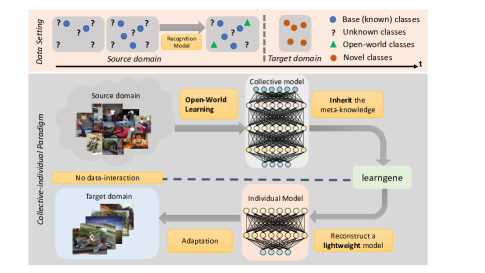
Figure 1: Approach Overview: Top row: The collective model is trained on continual learning tasks composed of base classes (as blue circles), and then recognize unknown classes (denoted by ‘?’) as open-world classes (green triangles, not belong to base classes), which are added to the training data incrementally. Finally, the individual model that inherits the meta-knowledge from the collective model adapts to the target tasks based on novel classes. Bottom row: The expandable collective model continuously deals with continual learning tasks and then recognize open-world classes. The lightweight individual model is initialized and reconstructed with learngene. The individual model adapts quickly to the target learning task even in the absence of the source data (no data-interaction).

Introduction

Over the past decade, deep learning has made significant progress on a fixed large-scale dataset or in a closed-world, where only the instances seen during training are presented to them. However, a network, trained in a specific task, is incapable of recognizing unknown/unseen classes due to domain shift (Ben-David et al. 2007) and category shift (Xu et al. 2018). Consequently, static and dedicated neural networks cannot resolve incrementally learning the unknown/unseen classes (Fei, Wang, and Liu 2016; Xu et al. 2019) without retraining from scratch and without catastrophic forgetting (French 1999), which is exactly what open-world learning (Bendale and Boult 2015; Shu, Xu, and Liu 2018) wants to solve. In addition, neural networks are typically over-parametrized (Han, Mao, and Dally 2016) and easily overfitting few samples (Wang et al. 2020).

There are currently some learning paradigms that can solve some of the above problems, such as continual learning (Hadsell et al. 2020), transfer learning (Perkins, Salomon et al. 1992) and meta-learning (Hospedales et al. 2020). Although continual learning can alleviate catastrophic forgetting by training on sequential tasks, the traditional continual learning cannot be reproduced in few samples. Many algorithms deal with category shift in transfer learning, which can reuse the model for the new task. In addition, meta-learning aims to design the model for learning prior knowledge of model parameters, so that new knowledge can be learned well from few samples. However, transfer learning comes across the dilemma of limited tasks, because it only focuses on the source tasks that transfer knowledge to the target tasks. Nevertheless, transfer learning and meta-learning perform inferior on the open-world tasks, as we discuss in Related Work section

Consequently, the above learning mechanisms are all limited. When we recall the learning process of biology, most of the behaviors of animals are congenital, not entirely through acquired learning. Besides, a recent neuroscience commentary, “What artificial neural networks (ANNs) can learn from animal brains” (Zador 2019) provides a critique of how rapid learning is currently implemented in ANNs. The innate knowledge comes from the universal genes (Zador 2019) of collective creatures that are constantly evolving. Afterwards, genes with certain rules flow to instantiated individuals, which enables them to learn very rapidly. Inspired by this, this paper is strongly motivated towards these goals of innate knowledge and learning. Specifically, the enlightenment for ANNs is that it is possible to design the expandable neural network (collective model) in the outer loop to train sequential tasks in the open-world, and then discover the critical modules through a judgment criterion of gradient information. The critical modules named learngene inherit meta-knowledge from the collective model. The lightweight network (individual model) is initialized and reconstructed from learngene. Finally, the individual model is retrained with few samples and adapt quickly to the novel classes without data- interaction of the collective model.

To verify this premise, we turn to training and analysis of expandable neural networks. As shown in Figure 1, we leverage the basic convolutional neural network (CNN) to set up the collective model, which automatically expands the network with different sequence tasks of base classes. The pretrained collective model recognizes unknown classes as open-world classes or base classes and incrementally adds them to training set. Afterwards, we propose the judgement criterion that the last/top $k$ network layers cover the meta-knowledge according to the changes of each layer of network parameters over time. Therefore, the $topk$ layers of the model are selected as the base modules of learngene. In other words, our paradigm replaces data-interaction with model interaction, thereby protecting the privacy of data. Besides, we employ the elastic weight consolidation (EWC) (Kirkpatrick et al. 2017) loss to retain the innate generalization ability as much as possible. Finally, through adjoining a small feature layer in front of the base module and thinner fully connected layers in the back, the individual model evaluates the learning ability on the target data of novel classes.

Contributions. (1) We propose a novel collective-individual paradigm, which is applicable for the practical scenario of continual open-world classification to reduce the sample and capacity cost of institutions or individuals without data-interaction. (2) To realize the collective-individual paradigm, we present learngene that inherits the meta-knowledge from the collective model and reconstructs a lightweight model for the target task. (3) We propose an effective criterion that can discover the learngene in the collective model, according to gradient information. (4) We demonstrate the effectiveness of our approach in an extensive empirical study and theoretical analysis.

Problem Setup

In this section, we describe the collective-individual paradigm and learngene that inherits the meta-knowledge from the collective model in the open-world and reconstructs a lightweight individual model for the target task.

Preliminaries

Notation. Let $\mathcal{X}$ and $\mathcal{Y}$ be a sample space and a label space, respectively. We refer to a pair of $\mathcal{Z}:=\mathcal{X}\times\mathcal{Y}$. In addition, let $\mathcal{H}=\{h:\mathcal{X}\rightarrow\mathcal{Y}\}$ be a hypothesis space and $\ell:\mathcal{Y}\times\mathcal{Y}\rightarrow\mathbb{R}^{+}$ represents a loss function. At any time $t$, we consider the set of known base classes as $\mathcal{C}^{t}=\{1,2,..,\mathrm{N}\}$ for the collective model. In order to realistically model the dynamics of the real-world case, we also assume that there exists a set of open-world classes $\mathcal{U}=\{\mathrm{N}+1,\ldots\}$, which could be encountered during inference. In addition, novel classes $\mathcal{N}=\{1,\ldots,K\}$ are different from previous classes, sampling for the reconstructed individual model.

Performance Measure. The fundamental purpose of the collective-individual model is to maximize the performance on the target task of novel classes. Therefore, a standard procedure is to empirically estimate by empirical risk estimator, i.e., $\widehat{er}(h):=\frac{1}{n}\sum_{j=1}^{n}\ell(h,\mathcal{N})$, where $n$ is number of the target tasks and $h$ is the individual model.

Table 1: Comparison of different task settings of collective-individual paradigm.

Task setting	No data-interaction	Open-world	Inheriting model to reconstruct lightweight model	Few samples adaptation
Transfer learning	$\surd$	$\times$	$\times$	$\times$
Continual learning	$\times$	$\surd$	$\times$	$\times$
Few-shot learning	$\surd$	$\times$	$\times$	$\surd$
Collective-individual paradigm	$\surd$	$\surd$	$\surd$	$\surd$

The Collective-individual Paradigm

Definition 1:

(collective-individual paradigm) The collective model can discriminate a test instance belonging to the known $\mathrm{N}$ classes, and also recognize an unknown or unseen instance by classifying it as an open-world or base class. Afterwards, the collective model incrementally adds $\mathrm{M}$ new classes and updates itself to produce a predicted model $\mathcal{M}_{\mathrm{N+M}}$ without retraining from scratch on the whole dataset. The known class set is updated $\mathcal{C}_{t+1}=\mathcal{C}_{t}+\{\mathrm{N+1},\ldots,\mathrm{N+M}\}$. In the collective-individual paradigm, a factory manufactures the collective model with base classes and open-world classes. The micro-institution or user trains the individual model initialized from learngene on the target learning task of novel classes.

Definition 2:

(Learngene) We formally define learngene as a rule $\phi$ for initializing the target model, inspired by (Zador 2019). Here we use gradient optimization rules to inherit important modules and parameters from the collective model and initialize the individual model.

Our paradigm has the following characteristics: i) No data-interaction: The individual model adapts to the target task in the absence of the source data, thereby protecting the privacy of data. Specifically, we allow category shift between the collective model and the individual model; ii) Open-world: The collective model adjusts scale to adapt to new tasks continuously and adds the unknown/unseen classes incrementally. The model preserves knowledge of previous tasks, i.e., factories or platforms produce large-scale model; iii) Inheriting model to reconstruct lightweight model: Inherit important modules and parameters from the collective model and initialize individual model; iv) few samples adaptation: Micro-institutions or users could train the individual model only with few samples on target learning tasks. We distinguish between the collective and individual model by adding a subscript col or idu to each notation introduced above (e.g., $\theta_{\mathrm{col}},\mathcal{D}^{idu}$).

Related Work

Transfer Learning

Methods such as (Huang et al. 2006; Sugiyama et al. 2008; Sun et al. 2011; Shen et al. 2018; Lee et al. 2019; Duan et al. 2009; Zhuang et al. 2009; Evgeniou, Micchelli, and Pontil 2005), which focus on transferring the knowledge across domains, aim at improving the performance of target learners in target domains. Compared with traditional transfer learning setting, our paradigm is not limited to static data, and has the ability to continuously recognize unknown/new classes. Moreover, continual domain adaptation (Zhao and Hoi 2010; Liu et al. 2020; Bitarafan, Baghshah, and Gheisari 2016; Wang, He, and Katabi 2020; Mancini et al. 2019a) enables the learner to adapt to continually evolving target domains without forgetting. However, this renders them impractical when deployed to the client because of model redundancy, while our method has no such restriction. Although meta domain adaptation (Balaji, Sankaranarayanan, and Chellappa 2018; Li et al. 2018; Sun et al. 2019) uses a lightweight model, it cannot continually learn new claases in an open-world environment.

Meta Learning

There is a three-way taxonomy across optimization-based methods (Finn, Abbeel, and Levine 2017; Shu et al. 2019), model-based methods (Ravi and Larochelle 2017; Santoro et al. 2016), and metric-based methods (Koch, Zemel, and Salakhutdinov 2015; Vinyals et al. 2016; Sung et al. 2018; Snell, Swersky, and Zemel 2017) in the meta-learning. They intend to design models as prior knowledge of learning model parameters that can learn new skills or adapt to new domain rapidly with few training examples. However, these approaches conventionally assumed that these tasks should be used together in batches, also called as few-shot learning, which are unable to train on sequential tasks. Although meta continual learning (Yao et al. 2020; Gidaris and Komodakis 2018; Jerfel et al. 2019; Javed and White 2019; Gupta, Yadav, and Paull 2020) can solve the sequential task problem by recording the efficiency task buffer, it still cannot prevent data-interaction. The collective-individual paradigm may not be referred to as meta-learning, but it may harness meta-learning across learning tasks, referred to as learning to learn. Thus, we set up some comparative experiments in the Experimental Results section.

Continual Learning

Continual learning (Parisi et al. 2019; De Lange et al. 2019; Kirkpatrick et al. 2017; Shin et al. 2017; Rusu et al. 2016; Rebuffi et al. 2017; Yoon et al. 2018; Xu and Zhu 2018) is also referred to as lifelong learning (Chen and Liu 2018; Aljundi, Chakravarty, and Tuytelaars 2017; Chaudhry et al. 2019), which aims to continually learn over time by accommodating new knowledge while retaining previously learned experiences. However, when data sharing is restricted due to its proprietary or privacy issues, this reliance on the coexistence of source data and target data is very impractical. Open-world learning (OWL, a.k.a. open world recognition or classification) (Bendale and Boult 2015; Mancini et al. 2019b; Shu, Xu, and Liu 2018) can be broadly defined as learning a model that can perform its intended task and then incrementally learn the new things. Furthermore, we solve the problem of transferring the meta-knowledge learned in the open-world to a practical lightweight model without data-interaction. Accordingly, a comparison of collective-individual paradigm with several different settings is provided in Table 3.

To sum up, our formulation of the collective-individual paradigm is different from prior arts. Not only can it recognize unknown/unseen classes in the open-world, but it can also adapt to new specific tasks by reconstructing and initializing a lightweight model based on few data of novel classes.

Methodology

Open-world Expandable/Collective Model

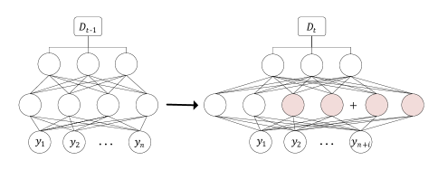
Figure 2: Expand the collective model. Left: The network trained on the $\mathcal{D}_{t-1}$. Right: The new task $\mathcal{D}_{t}$ contains $i$ new classes. When training on $\mathcal{D}_{t}$, copy the model modules in the red part and splice them together. The collective model supports deepening and widening operations.

Model Expansion

We presume that the model has a sequence of $T$ tasks, where the training data coming in at time $t$ is $D_{t}=\left\{\boldsymbol{x}_{i},y_{i}\right\}_{i=1}^{N_{t}}$. The tasks may contain new categories. Here we deliberate that each task is multi-class classification. When deepening the network, it arbitrarily duplicates the network of the previous layer to the following layer. Similarly, when the network is widened, a replica of the current layer can be randomly picked and then spliced together. Figure  2 describe the expanding process of the collective model. The network at all times before $t$ is trained on the data of $\mathcal{D}_{1},\ldots,\mathcal{D}_{t-1}$. When dealing with $D_{t}$, the network capacity demands to be increased to hold more knowledge of new tasks. Subsequently, network parameters are relevant to $\mathcal{D}_{1},\ldots,\mathcal{D}_{t}$. We train the network with the subsequent objective function:

$$\operatorname{minimize}_{\boldsymbol{W}_{F}^{t}}\mathcal{L}\left(\boldsymbol{W}_{F}^{t};\boldsymbol{W}_{F}^{t-1},\mathcal{D}_{t}\right),t=1,\ldots,T,$$ (1)

where $\mathcal{L}$ is a task-specific loss function(e.g., cross-entropy error function), $\boldsymbol{W}_{F}^{t}$ is the added parameter for task $t$, and $\boldsymbol{W}_{F}^{t-1}$ is the set of parameters copyed from the network at task $t-1$. We optimize the hyperparameters of the collective model by gradient descent.

Open-world Recognition

The collective model $\mathcal{M}_{\mathrm{N}}$ is trained on the tasks sampled from the base classes $\hat{\mathbf{Y}}^{\text{close }}$. More importantly, the collective model $\mathcal{M}_{\mathrm{N}}$ not only can discriminate a test instance belonging to the known $\mathrm{N}$ classes, but also recognize an unknown or unseen class instance by classifying it as an unknown. The unknown instance set $U$ can then be forwarded to a human user who can identify $\mathrm{M}$ new classes of interest (among a potentially large number of unknowns) and provide their training examples. The collective model incrementally adds $\mathrm{M}$ open-world classes and updates itself to generate a renewed model $\mathcal{M}_{\mathrm{N+M}}$, instead of learning from scratch on the full dataset. The known class set is also updated $C_{t+1}=C_{t}+\{\mathrm{N+1},...,\mathrm{N+M}\}$. This cycle continues over the life of the collective model, where it adaptively shapes itself with new knowledge. For an unknown instance, we use the following formula to calculate its open-world probability:

$$\hat{\mathbf{P}}=1-\max\frac{exp(f(x,y_{i};\theta_{col}))}{\sum_{j=1}^{N}exp(f(x,y_{j};\theta_{col}))}.$$ (2)

Based on $\hat{\mathbf{Y}}^{\text{close }}$ and $\hat{\mathbf{P}}$ , open-world pseudo label $\hat{\mathbf{Y}}^{\text{open }}$ is given as:

$$\hat{\mathbf{Y}}^{\text{open }}=\{\begin{array}[]{cl}C_{\text{open }}&\hat{\mathbf{P}}>\lambda_{\text{open }}\\ \hat{\mathbf{Y}}^{\text{close }}&\hat{\mathbf{P}}\leqslant\lambda_{\text{open }}\end{array}.$$ (3)

where $C_{open}$ denotes the open-world class, and $\lambda_{open}$ is the threshold to determine open-world instance. Therefore, the collective model is supposed to recognize a unknown or unseen class as well as incrementally adds it.

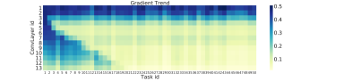
Figure 3: Gradient trends. The collective model handles 50 sequential tasks sampling from ImageNet. It shows the proportion of the large gradient from each model layer according to the judgment criterion. The gradient of each layer in the collective model trained with the open-world tasks reflects the number of parameter changes. The deeper network parameter changes tend to be stable with the task order, which is judged as the expected learngene.

Inheriting Learngene that Represents Meta-knowledge

In collective-individual paradigm, the primary challenge is to tackle how to determine the learngene by exploiting judgement criterion during training and the memorization effect of deep neural networks. Accordingly, learngene should have the ability to confirm critical modules and parameters across the tasks. Following this intuition, we design the criterion.

Judgement Criterion

For the optimization of the objective function $\mathcal{L}(\boldsymbol{W};\mathcal{D})$, the optimality will be achieved at $\boldsymbol{W}$ when $\nabla\mathcal{L}(\boldsymbol{W};\mathcal{D})=\mathbf{0}$ (Boyd, Boyd, and Vandenberghe 2004; Bubeck 2014). However, modern neural networks are complex and over-parameterized, which makes $\nabla\mathcal{L}(\boldsymbol{W};\mathcal{D})$ extremely high-dimensional. Optimality is difficult to judge effectively. To solve this problem, we use a more intuitive interpretation of the judgement criterion in this paper, so that optimization can be associated with a scalar. Every layer of our designed network is related to the data of $\mathcal{D}_{1},\ldots,\mathcal{D}_{t}$. Therefore, we analyze the gradient changes in the scalable neural network from the perspective of sequential tasks. Consider a parameter in one layer of the neural network, denoted by $\mathrm{w}_{i}\in\boldsymbol{W}$, its gradient is $\nabla\mathcal{L}\left(\mathrm{w}_{i};\mathcal{D}_{t}\right)$. Specifically, if we let

$$g_{i,t}=\left|\nabla\mathcal{L}\left(\mathrm{w}_{i};\mathcal{D}_{t}\right)\right|,i\in[m],t=1,\ldots$$ (4)

where $m$ represents the number of parameter in a certain layer. In this way, the judgement can be checked by exploiting the scalar $g_{i,t}$.

Inherting Learngene

We have shown that the optimization of the objective function can be related to a scalar $g_{i,t}$. There are three possible scenarios in open-world classification: (1) The parameters hardly change with the sequential task training, $g_{i,t}$ is always close to 0. (2) The parameters change drastically with the training of the sequence task, and $g_{i,t}$ is always large. (3) The gradient changes drastically and then stabilizes, that is, $g_{i,t}$ has a tendency to decrease and approach 0. Therefore, the judgement criterion is denoted by $\rho$, i.e.,

$$\rho=\frac{1}{m}\sum_{i=1}^{m}\Phi\left(g_{i,t}>\sigma\right),$$ (5)

where $\Phi$ return 1 if $g_{i,t}$ exceeds the threshold $\sigma$, and 0 otherwise. $\rho$ represents the proportion of the large gradient of a certain convolutional layer. If the value of $\rho$ is from large to steadily small, the network layer is viewed as candidate learngene, as it corresponds to the third scenario. As shown by Figure 3, the parameter changes of deeper network layers tend to be stable with the task order, which are judged as the expected learngene. Furthermore, We hypothesize that, the top layer is more inclined to learn the semantic-level information among tasks, i.e., meta-knowledge, after training numerous tasks in time series. On the contrary, the parameters of the front(bottom) layers change drastically, which corresponds to the second scenario. Because the bottom layers are sensitive to category shift and specific tasks.

Although the collective model is expandable, the individual model that inherits learngene does not need a enormous network to adapt to the target tasks with few samples. Specifically, with the judgement criterion, we reuse the $topk$ layers of the network, i.e., the deepest $k$ layers as the critical task-agnostic modules and parameters. Subsequently, the learngene is connected to the lightweight network layers for reconstructing the individual model.

Adapt Novel Classes with Few Samples

Algorithm 1 Adapt from the Collective Model

  Input: feature layers $F_{col}$ in the collective model, lightweight feature layers $F_{ind}$ in the individual model, classifier $C$ in the individual model, number of samples $\eta$ $F_{l}\leftarrow$ pick $topk$ layers in $F_{col}$individual model $\mathcal{M}$ $\leftarrow$ $\text{RECONSTRUCT}(F_{ind},F_{l},C)$parameter $\theta_{\mathcal{M}}$ of the model $\mathcal{M}$, weight factor $\lambda$

  for $i=1,\ldots,n$ do

     while $\mathcal{L}_{rec}+{\lambda}\mathcal{L}_{ret}$ has not converged do

        $(X_{c},Y_{c})\leftarrow$ batch sampled from $Q_{i}$

        $\widehat{Y}_{c}\leftarrow\mathcal{M}\left(X_{c}\right)$

        compute $\mathcal{L}_{rec}$ using Eq.  6

        $X_{p}$ batch sampled from $Q_{i}$

        for $x_{p}$ in $X_{p}$ do

           $\mathbf{L}\leftarrow$ $log\left[\sigma\left(\mathcal{M}(x_{p})\right)\right]$

           fisher matrix $F_{x}$ $\leftarrow\frac{\partial\mathbf{L}}{\partial x_{p}}$

        end for

        Compute $\mathcal{L}_{ret}$ using Eq.  8

        update $\theta_{\mathcal{M}}$ by minimizing Eq.  9

     end while

  end for

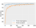
(a) Performance comparison on CIFAR100

(b) Performance comparison on ImageNet100

(c) Effect of number of samples on CIFAR100.

(d) Effect of number of samples on ImageNet100.

Figure 4: Comparison with learning from scratch. Figure (a) and (b) reveal that the individual model reconstructed by learngene reached a result close to convergence with averaged over 5 and 10 runs, and it is consistently higher than the one learned from scratch. Figure (c) and (d) show that the individual model requires far fewer samples to achieve fixed accuracy and perform much better with fewer samples than learning from scratch.

Due to the meta-knowledge of learngene from the collective model, the individual model greatly reduces the number of training samples. The adaptation contains two processes (see Algorithm 1): reconstruct and retain.

Reconstruct

The stage of adaptation allows the model to effectively respond to specific tasks of novel classes and reconstruct individual model based on learngene. We reuse the $topk$ modules and parameters of the collective model, which are connected to the smaller network layers. Therefore, the loss function of reconstruction is formulated as follows:

$$\mathcal{L}_{rec}=L_{\mathrm{ce}}(f(x;\theta_{ind}),\mathcal{Y}),$$ (6)

where $L_{\mathrm{ce}}$ is cross entropy loss.

Retain

The stage of inherting learngene decides to retain knowledge from the collective model. Retaining information of learngene can help the individual model to pass the early stage smoothly. At the same time, it is obligatory to maintain a certain degree of flexibility to adapt the network to new tasks. (Zador 2019) also emphasizes a similar balance between innate knowledge and acquired learning. Consequently, we regularize reused learngene to suppress the update of the parameters. Fisher information (Kirkpatrick et al. 2017) roughly measures the sensitivity of the model output distribution to small changes in parameters. For the supervised learning model $p_{\theta}\left(y|x\right)$, the fisher information matrix for a specific input $x$ is defined as follows:

$$F_{x}=\mathbb{E}_{p_{\theta}(y\mid x)}\left[\nabla_{\theta}\log p_{\theta}(y\mid x)\nabla_{\theta}\log p_{\theta}(y\mid x)^{\top}\right].$$ (7)

Therefore, using Fisher information as a secondary penalty, it penalizes the change of parameter distribution (measured by KL divergence). Limiting the slight changes in network parameters leads to the actual functional changes of the model also small. Given the fisher information matrix, the loss function of retaining $\mathcal{L}_{ret}$ is defined as

$$\mathcal{L}_{ret}=\sum_{i=n-k+1}^{n}\frac{1}{2}\left(F_{i}\left(\theta_{i}-\theta_{A,i}^{*}\right)^{2}\right).$$ (8)

$k$ means that only the $topk$ network layers are suppressed in the individual model, which is learngene inherited from the collective model. Finally, the loss function of the individual model is

$$\mathcal{L}=\mathcal{L}_{rec}+{\lambda}\mathcal{L}_{ret},$$ (9)

where $\lambda$ is the weighting parameter to trade-off between reconstruction and retaining.

Theoretical Analysis

Here, we present the theoretical analysis for transfering representation from collective model and get the following bound based on PAC-Bayesian (Pentina and Lampert 2014)
Theorem 1. For the prior $P$, we choose a Gaussian with zero mean and variance $\sigma I_{k}$. The posterior $Q$, is a shifted Gaussian with variance $\sigma I_{k}$ and mean $w_{Q}$ in the same subspace. The following bound holds for $t$ tasks

$$er(h)-\widehat{er}(h)<\frac{c_{2}}{2\sigma t\sqrt{\bar{m}}}+\mathit{c_{1}},$$ (10)

where $c_{1}$ and $c_{2}$ are all constants. $\bar{m}=\frac{1}{n}\sum_{i=1}^{n}{m_{i}}$ is the mean of the sample sizes. By inherting meta-knowledge from the collective model, we condition the individual model to satisfy Eq. 10, which is considered promising for target learning tasks. Since we use learngene to transfer representation from the collective model and initialize the individual model, the convergence rate of generalization error is bound. Note that, with increasing number of labeled target instances (increasing $\bar{m}$), the first term in Eq. 10 decreases. It explains that fewer samples are needed in the individual model to achieve better performance. In our formulation, this is achieved by enforcing $L_{rec}$, which can be regarded as a way to self-supervise the individual model.

Experiments

Experimental setting

Datasets. 1) CIFAR100. This dataset consists of 60, 000 images of 100 generic object classes (Krizhevsky, Hinton et al. 2009). The collective model uses 60 classes as base classes, 16 classes as open-world classes, and the remaining 20 classes as novel classes, to ensure no data-interaction between the two models. Five classes are randomly sampled for each continual learning task. 2) ImageNet100. This dataset has 14,197,122 images of 21841 labels (Russakovsky et al. 2014). Since the full ImageNet dataset is very large, we sub-sample 100 classes and conduct all experiments on this subset. Similarly, ImageNet100 is also divided into three parts and resizes 84 × 84 for each class.

Basic network. 1) Collective model. For experiments on the CIFAR100 and Imagenet100 datasets, we use thirteen convolutional layers as base network. The task data used by the collective model is inputted in chronological order. 2) Individual model. Considering the individual model is lightweight, we utilize seven convolutional layers, which the last three convolutional layers are inherited from the collective model. This individual model is adapted separately to target tasks of novel classes.

Hyperparameters. We set the learning rate to 0.001 and 0.005 when training the collective model and individual model, respectively. We fix all batch size to 32 and sample size in estimating fisher information to 128. $\lambda_{out}$ is 0.9587 for CIFAR100 and 0.9733 for Imagenet100 to achieve the best performance.

Experimental results and analysis

Evaluation on benchmark datasets. We report results on CIFAR100 and ImageNet100 datasets in Figure  4 (a) and (b). Learning curves in Figure  4 (a) show that the individual model is the fastest to adapt to new tasks in 10 epochs, averaging five target tasks. By contrast, Learning from scratch requires 40 epochs to converge. We also find that the individual model substantially outperforms the alternative approaches most of the time, confirming the useful knowledge inherited from the collective model. We hypothesize that, the learngene improve in efficiency over the course of learning as they see tasks previously. Besides, learngene has the ability to pay attention to meta-knowledge among tasks and generalize to novel classes. On the contrary, learning from scratch does not learn quickly compared to the individual model because there is no effective initialization rules.

Effect of number of training samples. We evaluate the effectiveness of the individual model from the perspective of samples. The results on CIFAR100 and ImageNet100 datasets are reported in Figure  4 (c) and (d). As shown in Figure  4 (c), the individual model only fits 25 samples to achieve 60% performance after 10 epochs. By contrast, Learning from scratch is overfitting such a small sample, and the gap is very obvious, where it attains at least 20% lower average accuracy. In addition, in abundant samples, the individual model has always performed better than learning from scratch. On the other hand, compared with learning from scratch, the individual model saves 2/3 of the sample and fine-tuning to 60% accuracy after 10 epochs. Furthermore, when the effect reaches 70% average accuracy, the individual model saves 100 samples for each class and extremely reduces the training samples for model. Therefore, it is possible to deploy the model to the personal user terminal.

Table 2: Multi-class classification accuracies on CIFAR100 and ImageNet100 with data of open-world classes.

Method	CIFAR100	ImageNet100
MAML	34.07$\pm$0.63	36.51$\pm$1.01
first-order MAML	25.40$\pm$0.50	32.82$\pm$0.65
PROTONET	33.20$\pm$0.48	36.26$\pm$0.32
PROTO-MAML	39.09$\pm$0.35	32.57$\pm$1.28
MATCHINGNET	34.99$\pm$0.34	37.79$\pm$0.39
Fine-tuning	38.72$\pm$1.13	40.72$\pm$1.36
Fine-tuning++	38.83$\pm$1.51	37.08$\pm$1.04
DEEPEMD	39.85$\pm$0.41	40.21$\pm$0.82
Ours	45.88$\pm$2.99	42.40$\pm$2.35

Open-world and novel classes with few samples. As aforementioned in the related work, we also conduct a comparative experiment on the data of open-world and novel classes. Tables 2 and 3 show the performance of our model from learngene against the few-shot learning algorithm with architectures of seven convolutional layers. Values represent average five classification accuracies obtained from the data of novel classes in 30 epochs and tested directly on the data of open-world classes. In order to ensure a fair comparison, we reset the capacity of the architectures of eight representative methods ((Finn, Abbeel, and Levine 2017; Nichol, Achiam, and Schulman 2018; Snell, Swersky, and Zemel 2017; Triantafillou et al. 2020; Vinyals et al. 2016; Zhang et al. 2020), two fine-tuning methods of (Chen et al. 2019)) to match ours on the data of novel classes. Our method can recognize unknown/unseen classes in the open-world scenario and incrementally add them. Still, the few-shot learning algorithm (trained on 20-shot) does not have this ability and can only directly test the open-world classes. As shown in the table 2, the collective model shows competitive results with open-world classes, achieving the best performance for all sample settings. For example, the individual model improves on average of a relative 6.03% wrt DeepEMD (the second-best method) with the data of open-world classes on CIFAR100. Despite its simplicity, table 3 shows that our proposed method achieves an average accuracy that, on CIFAR100 and ImageNet100 with data of novel classes, is superior to state of the art with the same architectures.

Table 3: Multi-class classification accuracies on CIFAR100 and ImageNet100 with data of novel classes.

	CIFAR100, 5way		ImageNet100, 5way
Method	10-shot	20-shot	10-shot	20-shot
MAML	51.70$\pm$1.75	62.36$\pm$2.88	48.62$\pm$3.10	57.62$\pm$2.42
first-order MAML	50.13$\pm$3.73	60.00$\pm$3.31	43.38$\pm$2.47	51.87$\pm$1.96
PROTONET	56.40$\pm$2.88	61.02$\pm$3.18	49.91$\pm$3.36	58.62$\pm$2.45
PROTO-MAML	53.11$\pm$1.25	59.57$\pm$1.34	45.14$\pm$2.52	53.57$\pm$1.34
MATCHINGNET	56.71$\pm$4.48	60.98$\pm$3.09	51.82$\pm$2.58	59.78$\pm$2.94
Fine-tuning	48.98$\pm$3.86	60.89$\pm$3.77	51.11$\pm$3.36	60.71$\pm$2.32
Fine-tuning++	52.67$\pm$4.02	61.20$\pm$3.29	40.80$\pm$2.92	51.78$\pm$2.81
DEEPEMD	58.03$\pm$1.85	63.69$\pm$2.05	50.93$\pm$2.78	59.69$\pm$2.47
Ours($\lambda=1000$)	58.86$\pm$3.12	64.24$\pm$1.89	52.96$\pm$4.84	60.86$\pm$4.48
Ours($\lambda=5000$)	58.21$\pm$2.58	63.74$\pm$2.46	52.53$\pm$4.74	59.76$\pm$5.41

Discussion

Evolution process of collective model. Intuitively, the collective model evolves (expands) (Stearns and Hoekstra 2000) on sequential tasks, and then the individual model reconstructed from learngene performs better over time. Inspired by this, we design an experiment to reconstruct multiple individual models with learngene, which is obtained from collective model trained along chronological order. The results (see Figure  6(a)) demonstrate that the individual model tends to perform better as the collective model continues to evolve (expand), since it alleviates catastrophic forgetting in the collective model and generate better meta-knowledge or semantic information. In the next subsection, we use visualization to explain this process.

Figure 5: Visualization for the collective model on unknown/unseen ImageNet samples. This figure analyzes that the collective model pays more attention the important position of the sample with sequential tasks training. For example, the first row reveals that the collective model gradually focuses on the harmonica in the lower right corner, when facial features and one hand interfere. Since the second and third rows of scenes are very similar, the model ultimately focuses on a similar semantic, such as the terrier.

Why is learngene needed? We further discuss the interpretability of learngene through visualization (Selvaraju et al. 2017), derived from the output of top convolutional layer in the collective model. We use the other classes in ImageNet to visualize in the training process of the collective model. Since the collective model is continuously trained, Figure  5 shows that the model pays more attention to the position of the similar semantic information for the unseen classes. Therefore, learngene inherited from the collective model also has the ability to aid the individual model in quickly distinguishing the unseen categories, which also explains why unknown instances can be recognized.

(a) Evolution (Expansion) of the collective model

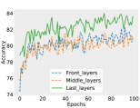
(b) Evaluation on judgement criterion

Figure 6: Figure (a) reveals that the performance of the individual model continually improves, as the collective model is trained on sequence tasks. Figure (b) further verifies the rationality of judgement criterion for obtaining learngene.

Evaluation on judgement criterion. In order to further confirm the learngene proposed by our judgement criterion, we design a network with the same capacity for each layer. The network is also trained on sequence tasks. Thereafter, we squeeze the front, middle and top three areas of the network to reconstruct the individual model. Figure  6(b) shows that the individual model inheriting learngene from the top position of the network is stable and finally 2% accuracy higher than other locations. Accordingly, since the top network layers can better capture semantic information or meta-knowledge between tasks, the individual model reconstructed by learngene can adapt to the target tasks more quickly and has better generalization performance.

Conclusion

In this paper, we propose a practical collective-individual paradigm. Furthermore, we introduce the learngene that inherits the meta-knowledge from the collective model in the open-world scenario and reconstructs a new lightweight model for the target task. We use a novel and effective criterion to discover learngene based on gradient information. Through extensive empirical evaluation and theoretical analysis, we demonstrate the effectiveness of our approach. As future work, networks of different structures (e.g. Resnet (He et al. 2016)) and automatically inherit learngene as the initialization rule of the target task are worth exploration.

References

- Aljundi, Chakravarty, and Tuytelaars (2017) Aljundi, R.; Chakravarty, P.; and Tuytelaars, T. 2017. Expert Gate: Lifelong Learning with a Network of Experts. In CVPR, 7120–7129. IEEE Computer Society.
- Balaji, Sankaranarayanan, and Chellappa (2018) Balaji, Y.; Sankaranarayanan, S.; and Chellappa, R. 2018. MetaReg: Towards Domain Generalization using Meta-Regularization. In NeurIPS, 1006–1016.
- Ben-David et al. (2007) Ben-David, S.; Blitzer, J.; Crammer, K.; Pereira, F.; et al. 2007. Analysis of representations for domain adaptation. In NeurIPS, 19: 137.
- Bendale and Boult (2015) Bendale, A.; and Boult, T. E. 2015. Towards Open World Recognition. In CVPR, 1893–1902. IEEE Computer Society.
- Bitarafan, Baghshah, and Gheisari (2016) Bitarafan, A.; Baghshah, M. S.; and Gheisari, M. 2016. Incremental Evolving Domain Adaptation. IEEE Trans. Knowl. Data Eng., 28(8): 2128–2141.
- Boyd, Boyd, and Vandenberghe (2004) Boyd, S.; Boyd, S. P.; and Vandenberghe, L. 2004. Convex optimization. Cambridge university press.
- Bubeck (2014) Bubeck, S. 2014. Convex optimization: Algorithms and complexity. arXiv preprint arXiv:1405.4980.
- Chaudhry et al. (2019) Chaudhry, A.; Ranzato, M.; Rohrbach, M.; and Elhoseiny, M. 2019. Efficient Lifelong Learning with A-GEM. In ICLR.
- Chen et al. (2019) Chen, W.; Liu, Y.; Kira, Z.; Wang, Y. F.; and Huang, J. 2019. A Closer Look at Few-shot Classification. In ICLR.
- Chen and Liu (2018) Chen, Z.; and Liu, B. 2018. Lifelong Machine Learning, Second Edition. Synthesis Lectures on Artificial Intelligence and Machine Learning. Morgan & Claypool Publishers.
- De Lange et al. (2019) De Lange, M.; Aljundi, R.; Masana, M.; Parisot, S.; Jia, X.; Leonardis, A.; Slabaugh, G.; and Tuytelaars, T. 2019. A continual learning survey: Defying forgetting in classification tasks. arXiv preprint arXiv:1909.08383.
- Duan et al. (2009) Duan, L.; Tsang, I. W.; Xu, D.; and Chua, T.-S. 2009. Domain adaptation from multiple sources via auxiliary classifiers. In ICML, 289–296.
- Evgeniou, Micchelli, and Pontil (2005) Evgeniou, T.; Micchelli, C. A.; and Pontil, M. 2005. Learning multiple tasks with kernel methods. Journal of machine learning research, 6(Apr): 615–637.
- Fei, Wang, and Liu (2016) Fei, G.; Wang, S.; and Liu, B. 2016. Learning Cumulatively to Become More Knowledgeable. In Proceedings of the 22nd ACM SIGKDD International Conference on Knowledge Discovery and Data Mining, San Francisco, CA, USA, August 13-17, 2016, 1565–1574. ACM.
- Finn, Abbeel, and Levine (2017) Finn, C.; Abbeel, P.; and Levine, S. 2017. Model-Agnostic Meta-Learning for Fast Adaptation of Deep Networks. In ICML, volume 70 of Proceedings of Machine Learning Research, 1126–1135. PMLR.
- French (1999) French, R. M. 1999. Catastrophic forgetting in connectionist networks. Trends in cognitive sciences, 3(4): 128–135.
- Gidaris and Komodakis (2018) Gidaris, S.; and Komodakis, N. 2018. Dynamic few-shot visual learning without forgetting. In CVPR, 4367–4375.
- Gupta, Yadav, and Paull (2020) Gupta, G.; Yadav, K.; and Paull, L. 2020. Look-ahead Meta Learning for Continual Learning. In NeurIPS.
- Hadsell et al. (2020) Hadsell, R.; Rao, D.; Rusu, A. A.; and Pascanu, R. 2020. Embracing Change: Continual Learning in Deep Neural Networks. Trends in Cognitive Sciences, 24(12): 1028–1040.
- Han, Mao, and Dally (2016) Han, S.; Mao, H.; and Dally, W. J. 2016. Deep Compression: Compressing Deep Neural Network with Pruning, Trained Quantization and Huffman Coding. In ICLR.
- He et al. (2016) He, K.; Zhang, X.; Ren, S.; and Sun, J. 2016. Deep Residual Learning for Image Recognition. In CVPR, 770–778. IEEE Computer Society.
- Hospedales et al. (2020) Hospedales, T. M.; Antoniou, A.; Micaelli, P.; and Storkey, A. J. 2020. Meta-Learning in Neural Networks: A Survey. CoRR, abs/2004.05439.
- Huang et al. (2006) Huang, J.; Gretton, A.; Borgwardt, K.; Schölkopf, B.; and Smola, A. 2006. Correcting sample selection bias by unlabeled data. In NeurIPS, 19: 601–608.
- Javed and White (2019) Javed, K.; and White, M. 2019. Meta-Learning Representations for Continual Learning. In NeurIPS, 1818–1828.
- Jerfel et al. (2019) Jerfel, G.; Grant, E.; Griffiths, T.; and Heller, K. A. 2019. Reconciling meta-learning and continual learning with online mixtures of tasks. In NeurIPS, 9119–9130.
- Kirkpatrick et al. (2017) Kirkpatrick, J.; Pascanu, R.; Rabinowitz, N.; Veness, J.; Desjardins, G.; Rusu, A. A.; Milan, K.; Quan, J.; Ramalho, T.; Grabska-Barwinska, A.; et al. 2017. Overcoming catastrophic forgetting in neural networks. Proceedings of the national academy of sciences, 114(13): 3521–3526.
- Koch, Zemel, and Salakhutdinov (2015) Koch, G.; Zemel, R.; and Salakhutdinov, R. 2015. Siamese neural networks for one-shot image recognition. In ICML deep learning workshop, volume 2. Lille.
- Krizhevsky, Hinton et al. (2009) Krizhevsky, A.; Hinton, G.; et al. 2009. Learning multiple layers of features from tiny images.
- Lee et al. (2019) Lee, C.-Y.; Batra, T.; Baig, M. H.; and Ulbricht, D. 2019. Sliced wasserstein discrepancy for unsupervised domain adaptation. In CVPR, 10285–10295.
- Li et al. (2018) Li, D.; Yang, Y.; Song, Y.; and Hospedales, T. M. 2018. Learning to Generalize: Meta-Learning for Domain Generalization. In AAAI, 3490–3497. AAAI Press.
- Liu et al. (2020) Liu, H.; Long, M.; Wang, J.; and Wang, Y. 2020. Learning to Adapt to Evolving Domains. In NeurIPS.
- Mancini et al. (2019a) Mancini, M.; Bulò, S. R.; Caputo, B.; and Ricci, E. 2019a. AdaGraph: Unifying Predictive and Continuous Domain Adaptation Through Graphs. In CVPR, 6568–6577. Computer Vision Foundation / IEEE.
- Mancini et al. (2019b) Mancini, M.; Karaoguz, H.; Ricci, E.; Jensfelt, P.; and Caputo, B. 2019b. Knowledge is Never Enough: Towards Web Aided Deep Open World Recognition. In ICRA, 9537–9543. IEEE.
- Nichol, Achiam, and Schulman (2018) Nichol, A.; Achiam, J.; and Schulman, J. 2018. On First-Order Meta-Learning Algorithms. CoRR, abs/1803.02999.
- Parisi et al. (2019) Parisi, G. I.; Kemker, R.; Part, J. L.; Kanan, C.; and Wermter, S. 2019. Continual lifelong learning with neural networks: A review. Neural Networks, 113: 54–71.
- Pentina and Lampert (2014) Pentina, A.; and Lampert, C. H. 2014. A PAC-Bayesian bound for Lifelong Learning. In ICML, volume 32 of JMLR Workshop and Conference Proceedings, 991–999.
- Perkins, Salomon et al. (1992) Perkins, D. N.; Salomon, G.; et al. 1992. Transfer of learning. International encyclopedia of education, 2: 6452–6457.
- Ravi and Larochelle (2017) Ravi, S.; and Larochelle, H. 2017. Optimization as a Model for Few-Shot Learning. In ICLR.
- Rebuffi et al. (2017) Rebuffi, S.-A.; Kolesnikov, A.; Sperl, G.; and Lampert, C. H. 2017. icarl: Incremental classifier and representation learning. In CVPR, 2001–2010.
- Russakovsky et al. (2014) Russakovsky, O.; Deng, J.; Su, H.; Krause, J.; Satheesh, S.; Ma, S.; Huang, Z.; Karpathy, A.; Khosla, A.; Bernstein, M. S.; Berg, A. C.; and Li, F. 2014. ImageNet Large Scale Visual Recognition Challenge. CoRR, abs/1409.0575.
- Rusu et al. (2016) Rusu, A. A.; Rabinowitz, N. C.; Desjardins, G.; Soyer, H.; Kirkpatrick, J.; Kavukcuoglu, K.; Pascanu, R.; and Hadsell, R. 2016. Progressive neural networks. arXiv preprint arXiv:1606.04671.
- Santoro et al. (2016) Santoro, A.; Bartunov, S.; Botvinick, M.; Wierstra, D.; and Lillicrap, T. 2016. Meta-learning with memory-augmented neural networks. In ICML, 1842–1850.
- Selvaraju et al. (2017) Selvaraju, R. R.; Cogswell, M.; Das, A.; Vedantam, R.; Parikh, D.; and Batra, D. 2017. Grad-CAM: Visual Explanations from Deep Networks via Gradient-Based Localization. In ICCV, 618–626. IEEE Computer Society.
- Shen et al. (2018) Shen, J.; Qu, Y.; Zhang, W.; and Yu, Y. 2018. Wasserstein Distance Guided Representation Learning for Domain Adaptation. In AAAI.
- Shin et al. (2017) Shin, H.; Lee, J. K.; Kim, J.; and Kim, J. 2017. Continual Learning with Deep Generative Replay. In NeurIPS, 2990–2999.
- Shu et al. (2019) Shu, J.; Xie, Q.; Yi, L.; Zhao, Q.; Zhou, S.; Xu, Z.; and Meng, D. 2019. Meta-Weight-Net: Learning an Explicit Mapping For Sample Weighting. In NeurIPS, 1917–1928.
- Shu, Xu, and Liu (2018) Shu, L.; Xu, H.; and Liu, B. 2018. Unseen Class Discovery in Open-world Classification. CoRR, abs/1801.05609.
- Snell, Swersky, and Zemel (2017) Snell, J.; Swersky, K.; and Zemel, R. 2017. Prototypical networks for few-shot learning. In NeurIPS, 4077–4087.
- Stearns and Hoekstra (2000) Stearns, S. C.; and Hoekstra, R. F. 2000. Evolution, an introduction. Oxford University Press.
- Sugiyama et al. (2008) Sugiyama, M.; Suzuki, T.; Nakajima, S.; Kashima, H.; von Bünau, P.; and Kawanabe, M. 2008. Direct importance estimation for covariate shift adaptation. Annals of the Institute of Statistical Mathematics, 60(4): 699–746.
- Sun et al. (2011) Sun, Q.; Chattopadhyay, R.; Panchanathan, S.; and Ye, J. 2011. A two-stage weighting framework for multi-source domain adaptation. In NeurIPS, 24: 505–513.
- Sun et al. (2019) Sun, Q.; Liu, Y.; Chua, T.-S.; and Schiele, B. 2019. Meta-Transfer Learning for Few-Shot Learning. 2019 IEEE/CVF Conference on Computer Vision and Pattern Recognition (CVPR), 403–412.
- Sung et al. (2018) Sung, F.; Yang, Y.; Zhang, L.; Xiang, T.; Torr, P. H.; and Hospedales, T. M. 2018. Learning to compare: Relation network for few-shot learning. In CVPR, 1199–1208.
- Triantafillou et al. (2020) Triantafillou, E.; Zhu, T.; Dumoulin, V.; Lamblin, P.; Evci, U.; Xu, K.; Goroshin, R.; Gelada, C.; Swersky, K.; Manzagol, P.-A.; and Larochelle, H. 2020. Meta-Dataset: A Dataset of Datasets for Learning to Learn from Few Examples. In International Conference on Learning Representations.
- Vinyals et al. (2016) Vinyals, O.; Blundell, C.; Lillicrap, T.; Wierstra, D.; et al. 2016. Matching networks for one shot learning. In NeurIPS, 29: 3630–3638.
- Wang, He, and Katabi (2020) Wang, H.; He, H.; and Katabi, D. 2020. Continuously Indexed Domain Adaptation. In ICML, volume 119 of Proceedings of Machine Learning Research, 9898–9907. PMLR.
- Wang et al. (2020) Wang, Y.; Yao, Q.; Kwok, J. T.; and Ni, L. M. 2020. Generalizing from a few examples: A survey on few-shot learning. ACM Computing Surveys (CSUR), 53(3): 1–34.
- Xu et al. (2019) Xu, H.; Liu, B.; Shu, L.; and Yu, P. S. 2019. Open-world Learning and Application to Product Classification. In In WWW, 3413–3419. ACM.
- Xu and Zhu (2018) Xu, J.; and Zhu, Z. 2018. Reinforced Continual Learning. In Bengio, S.; Wallach, H.; Larochelle, H.; Grauman, K.; Cesa-Bianchi, N.; and Garnett, R., eds., Advances in Neural Information Processing Systems, volume 31. Curran Associates, Inc.
- Xu et al. (2018) Xu, R.; Chen, Z.; Zuo, W.; Yan, J.; and Lin, L. 2018. Deep cocktail network: Multi-source unsupervised domain adaptation with category shift. In CVPR, 3964–3973.
- Yao et al. (2020) Yao, H.; Zhou, Y.; Mahdavi, M.; Li, Z.; Socher, R.; and Xiong, C. 2020. Online Structured Meta-learning. In NeurIPS.
- Yoon et al. (2018) Yoon, J.; Yang, E.; Lee, J.; and Hwang, S. J. 2018. Lifelong Learning with Dynamically Expandable Networks. In ICLR.
- Zador (2019) Zador, A. M. 2019. A critique of pure learning and what artificial neural networks can learn from animal brains. Nature communications, 10(1): 1–7.
- Zhang et al. (2020) Zhang, C.; Cai, Y.; Lin, G.; and Shen, C. 2020. DeepEMD: Few-Shot Image Classification With Differentiable Earth Mover’s Distance and Structured Classifiers. 2020 IEEE/CVF Conference on Computer Vision and Pattern Recognition (CVPR), 12200–12210.
- Zhao and Hoi (2010) Zhao, P.; and Hoi, S. C. H. 2010. OTL: A Framework of Online Transfer Learning. In ICML, 1231–1238. Omnipress.
- Zhuang et al. (2009) Zhuang, F.; Luo, P.; Xiong, H.; Xiong, Y.; He, Q.; and Shi, Z. 2009. Cross-domain learning from multiple sources: A consensus regularization perspective. In TKDE, 22(12): 1664–1678.