A decreasing scaling transition scheme from Adam to SGD

Abstract

Adaptive gradient algorithm (AdaGrad) and its variants, such as RMSProp, Adam, AMSGrad, etc, have been widely used in deep learning. Although these algorithms are faster in the early phase of training, their generalization performance is often not as good as stochastic gradient descent (SGD). Hence, a trade-off method of transforming Adam to SGD after a certain iteration to gain the merits of both algorithms is theoretically and practically significant. To that end, we propose a decreasing scaling transition scheme to achieve a smooth and stable transition from Adam to SGD, which is called DSTAdam. The convergence of the proposed DSTAdam is also proved in an online convex setting. Finally, the effectiveness of the DSTAdam is verified on the CIFAR-10/100 datasets. Our implementation is available at: https://github.com/kunzeng/DSTAdam.

1 Introduction

Deep neural networks (DNN) have achieved great success in many fields, such as computer vision[1], natural language translation[2], medical treatment[3] and transportation[4]. Many popular neural network models have been proposed, such as fully connected neural network[5], LeNet[6], LSTM[7], ResNet[8], DensNet[9], etc. During the training of these models, the optimization algorithms always play a significant role. One of the most dominant algorithms is stochastic gradient descent (SGD) [10] with a simple mathematical form and low computational complexity. However, SGD only depends on the current stochastic gradient and is not stable enough in the training process. Polyak et al.[11] added a momentum term into SGD and employed a constant learning rate to scale the gradient in all directions. Duchi et al.[12] proposed an adaptive gradient (AdaGrad) algorithm with the second moment as the adaptive learning rate. Furthermore, there are many variants of AdaGrad, such as RMSProp[13], AdaDelta[14] and Adam [15]. Adam is a combination of AdaGrad and RMSProp, which has been widely used into various deep neural networks. Reddi et al.[16] found that Adam could not converge for a convex optimization problem, and proposed AMSGrad to make up for this deficiency.

Another methodology is to transform Adam to SGD in the later stages of training [17, 18, 19, 20, 21], which can have the advantages of rapid convergence of Adam and good generalization of SGD. In particular, we would like to point out that Keskar et al.[17] manually switched Adam to SGD after a certain moment in the training process, which satisfies the conditions $\displaystyle k>1$ and $\displaystyle\left|{{\lambda_{k}}/\left({1-\beta_{2}^{k}}\right)-{\gamma_{k}}}\right|<\varepsilon$. However, it is difficult to obtain the optimal transition moment for the “hard” transition in practice. Luo et al.[18] investigated the extreme learning rates of Adam and proposed an adaptive gradient algorithm with two dynamic bound functions (named AdaBound) to achieve a smooth transition from Adam to SGD. However, AdaBound is data-independent on the chosen bound functions and may hurt the generalization performanc[20]. Therefore, how to achieve a better transition from Adam to SGD still needs more and further investigation.

In this paper, we firstly introduce a general transition framework and propose a decreasing scaling scheme to achieve a smooth and stable transition from Adam to SGD. Through the scaling, the adaptability of Adam is retained to some extent during the transition process. In the training stage of SGD, we employ linear decreasing learning rate instead of a constant learning rate to obtain better experimental results. Furthermore, we prove that DSTAdam has a regret bound $\displaystyle\mathcal{O}({\sqrt{T}})$ in the online convex setting. Experimental results show that the proposed DSTAdam has faster convergence speed and better generalization performance.

2 Preliminaries

Notation. For $\displaystyle x\in{\mathbb{R}^{d}}$, we use $\displaystyle{x_{i}}$ to denote the $\displaystyle i$-th component of vector $\displaystyle x$. $\displaystyle{\left\|x\right\|_{2}}$ and $\displaystyle{\left\|x\right\|_{\infty}}$ respectively denote the $\displaystyle{l_{2}}$-norm and $\displaystyle{l_{\infty}}$-norm of $\displaystyle x$. For any two vectors $\displaystyle x,y\in{\mathbb{R}^{d}}$, $\displaystyle\left\langle{x,y}\right\rangle$ signifies the inner product. $\displaystyle xy$ and $\displaystyle x/y$ denote element-wise product and element-wise division respectively. $\displaystyle\mathcal{S}_{+}^{d}$ means the set of all positive definite $\displaystyle d\times d$ matrices. For a vector $\displaystyle a\in\mathbb{R}^{d}$ and a positive definite matrix $\displaystyle M\in\mathbb{R}^{d\times d}$, we use $\displaystyle a/M$ to denote $\displaystyle M^{-1}a$ and $\displaystyle\sqrt{M}$ to denote $\displaystyle M^{1/2}$. The projection operation $\displaystyle\Pi_{\mathcal{F},M}(y)$ for $\displaystyle M\in\mathcal{S}_{+}^{d}$ is defined as $\displaystyle\arg\min_{x\in\mathcal{F}}\left\|M^{1/2}(x-y)\right\|$ for $\displaystyle y\in\mathbb{R}^{d}$. The set $\displaystyle\{1,2,\cdots,T\}$ is denoted as $\displaystyle[T]$ .

Algorithm 1 Generic framework of transition methods

Input: $\displaystyle\theta_{1}\in\mathcal{F}$, step size $\displaystyle\{\eta_{t}\}_{t=1}^{T}$, sequence of functions $\displaystyle\{\phi_{t},\psi_{t}\}_{t=1}^{T}$, bound functions $\displaystyle\eta_{l}$ and $\displaystyle\eta_{u}$.

1:for $\displaystyle t=1$ to $\displaystyle T$ do

2:     Generate a stochastic gradient $\displaystyle{g_{t}}=\nabla{f_{t}}({\theta_{t}})$

3:     $\displaystyle m_{t}=\phi_{t}\left(g_{1},\ldots,g_{t}\right)\text{\ }and\ v_{t}=\psi_{t}\left(g_{1},\ldots,g_{t}\right)$

4:     $\displaystyle{\eta_{t}}=\text{Clip}\left({\alpha/\sqrt{{v_{t}}},{\eta_{l}}\left(t\right),{\eta_{u}}\left(t\right)}\right)$

5:     $\displaystyle\theta_{t+1}=\Pi_{\mathcal{F},\operatorname{diag}\left(\eta_{t}^{-1}\right)}\left(\theta_{t}-\eta_{t}m_{t}\right)$

6:end for

Optimization problem. In the online learning framework [22], the sequence of convex loss function is defined as $\displaystyle{f_{1}}\left({{\theta_{1}}}\right),{f_{2}}\left({{\theta_{2}}}\right),...,{f_{T}}\left({{\theta_{T}}}\right)$, where $\displaystyle{\theta_{t}}$ is the parameter that needs to be optimized. Then, the regret of the problem is defined as the sum of the difference between each iteration loss and the optimal loss [23], that is

$$R(T)=\sum\limits_{t=1}^{T}{\left({{f_{t}}({\theta_{t}})-{f_{t}}\left({{\theta^{*}}}\right)}\right)},$$ (1)

where $\displaystyle{\theta^{*}}=\arg\min_{\theta\in\mathcal{F}}\sum\nolimits_{t=1}^{T}{f_{t}}(\theta)$. Throughout this paper, we assume that the feasible set $\displaystyle\mathcal{F}$ has bounded diameter $\displaystyle{D_{\infty}}$ such that $\displaystyle\left\|{x-y}\right\|\leq{D_{\infty}}$, $\displaystyle\forall x,y\in\mathcal{F}$.

A generic overview of transition methods. Following the clipping operation of [18], we now provide a generic framework of transition methods in Algorithm 1, which encapsulates many popular transition methods so that we can better understand the differences between different transition methods. In Algorithm 1, $\displaystyle\phi_{t}$ and $\displaystyle\psi_{t}$ denote the ”averaging” functions which have not been specified, $\displaystyle\eta_{l}(t)$ and $\displaystyle\eta_{u}(t)$ denote the lower and upper bound functions. Based on such a framework, we have listed most of the existing bound functions in Table 1.

Table 1: Some bound functions

$\displaystyle\eta_{l}(t)$	$\displaystyle\eta_{u}(t)$	References
$\displaystyle\alpha^{*}$	$\displaystyle\alpha^{*}$	[17]
$\displaystyle\alpha^{*}\left(1-\frac{1}{\left(1-\beta_{2}\right)t+1}\right)$	$\displaystyle\alpha^{*}\left(1+\frac{1}{\left(1-\beta_{2}\right)t}\right)$	[18, 19]
$\displaystyle\alpha^{*}$	$\displaystyle\alpha^{*}+\frac{\left|m_{t}\right|}{\max\left\{\left|m_{t}\right|\right\}\cdot(\gamma t)}$	[20]
$\displaystyle\alpha^{*}\cdot\frac{t}{T}$	$\displaystyle\alpha^{*}+\frac{1}{\left(1-\beta_{2}\right)\cdot t}-\frac{1}{\left(1-\beta_{2}\right)\cdot T}$	[21]

From Table 1, we can see that most of the existing transition methods from adaptive gradient descent to stochastic gradient descent are improvement on the lower and upper bound functions of clipping operation, but there are few studies on such transition operation.

3 DSTAdam algorithm

In this section, we propose a new transition method from Adam to SGD. For the SGD algorithm, we make use of linear decreasing learning rate to accelerate the training speed in the early stage and stabilize the convergence in the later stage. A scaling function $\displaystyle\rho_{t}$ is introduced to gradually scale the adaptive learning rate to the linear decreasing learning rate, which retains the adaptability of Adam to a certain extent, and achieves a smooth and stable transition from Adam to SGD. The specific algorithm is described in Algorithm 2.

Algorithm 2 Decreasing Scaling Transition from Adam to SGD (DSTAdam) Algorithm

Input: $\displaystyle\theta_{1}\in\mathcal{F}$, initial step size $\displaystyle\alpha$, $\displaystyle r_{l}$, $\displaystyle r_{u}$, $\displaystyle\{{\rho_{t}}\}$, $\displaystyle\{{\beta_{1t}}\}$ and $\displaystyle\{{\beta_{2t}}\}$.
Initialize: $\displaystyle m_{0}=0,v_{0}=0.$

1:for $\displaystyle t=1$ to $\displaystyle T$ do

2:     $\displaystyle{g_{t}}=\nabla{f_{t}}({\theta_{t}})$

3:     $\displaystyle{m_{t}}={\beta_{1t}}{m_{t-1}}+(1-{\beta_{1t}}){g_{t}}$

4:     $\displaystyle{v_{t}}={\beta_{2t}}{v_{t-1}}+(1-{\beta_{2t}})g_{t}^{2}$

5:     $\displaystyle{r_{t}}=\left({r_{u}-r_{l}}\right)(1-t/T)+r_{l}$

6:     $\displaystyle{\hat{\eta}_{t}}=\rho_{t}\left({\alpha/\sqrt{{v_{t}}}-{r_{t}}}\right)+{r_{t}}$ and $\displaystyle\eta_{t}=\hat{\eta}_{t}/\sqrt{t}$

7:     $\displaystyle\theta_{t+1}=\Pi_{\mathcal{F},\operatorname{diag}\left(\eta_{t}^{-1}\right)}\left(\theta_{t}-\eta_{t}m_{t}\right)$

8:end for

For the sake of clarity, we omit the bias correction operations of the first and second moments in DSTAdam. Following the hyperparameter setting of Adam [15], the hyperparameters of DSTAdam are taken as $\displaystyle\alpha=0.001$, $\displaystyle{\beta_{1t}}=0.9$ and $\displaystyle{\beta_{2t}}=0.999$. In a similar manner as [18], we set $\displaystyle\eta_{t}=\hat{\eta}_{t}/\sqrt{t}$ for theoretical analysis, but $\displaystyle\eta_{t}=\hat{\eta}_{t}$ is more effective in practice.

Remark 3.1

It should be noted that the transition steps 5-6 of Algorithm 2 is more smooth and stable through the scaling operation instead of the clipping operation. This technology effectively reduces the dependence of AdaBound on the bound functions and restores the element-to-element operation of the effective learning rates. The schematic diagrams of the learning rates distribution of the training process of Adam, AdaBound and DSTAdam for ResNet-18 on CIFAR-10 are shown in Fig. 1, where the $\displaystyle x$-axis is scaled by log function and the $\displaystyle y$-axis denotes the number of iterations. We can see that $\displaystyle i$) the learning rates of Adam are widely distributed, and there are a lot of extreme learning rates in the later stage of training, $\displaystyle ii$) the learning rates of the AdaBound quickly shrink to a small interval after a few iterations due to the clipping operation of two bound functions of AdaBound, and $\displaystyle iii$) the learning rates of the DSTAdam are similar to that of Adam in the early stage of training, and its learning rates gradually transform to a small range with the number of iterations. In contrast to Adam and AdaBound, the transition process of DSTAdam eliminates extreme learning rates while retaining its adaptability to a certain extent.

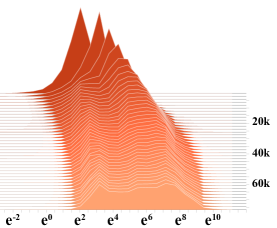
(a) Learning rates of Adam.

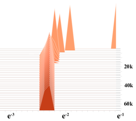
(b) Learning rates of AdaBound.

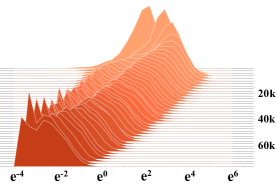
(c) Learning rates of DSTAdam.

Figure 1: The schematic diagrams of the learning rates distribution of the Adam, AdaBound and DSTAdam

4 Convergence Analysis of DSTAdam

Under the similar conditions as [15, 18, 16, 24], we obtain the following convergence theorem for the DSTAdam, and its proof is given in the Appendix A.

Theorem 4.1

Let $\displaystyle\left\{{{\theta_{t}}}\right\}$ and $\displaystyle\left\{{{\eta_{t}}}\right\}$ be the sequence generated by DSTAdam, $\displaystyle{\rho_{t}}\leq\rho$, $\displaystyle\rho\in\left({0,1}\right)$, $\displaystyle\eta_{t}=\hat{\eta}_{t}/\sqrt{t}$, $\displaystyle r_{l}\leq r_{u}$, $\displaystyle{\beta_{1t}}\leq{\beta_{1}}$ for all $\displaystyle t\in\left[T\right]$, $\displaystyle{\beta_{1}}\in\left[{0,1}\right)$. Assume that $\displaystyle\left\|x-y\right\|_{\infty}\leq D_{\infty}$, $\displaystyle\forall x,y\in\mathcal{F}$ and $\displaystyle\left\|\nabla f_{t}(\theta)\right\|_{\infty}\leq G_{\infty}$, $\displaystyle\forall t\in\left[T\right]$ and $\displaystyle\forall\theta\in\mathcal{F}$. Furthermore, let $\displaystyle\left\{\beta_{2t}\right\}$ be such that the following conditions are satisfied:

$$\textbf{(C1). }\sqrt{t\sum_{j=1}^{t}\prod_{k=1}^{t-j}\beta_{2(t-k+1)}\left(1-\beta_{2j}\right)g_{j,i}^{2}}\geq\frac{1}{\zeta}\sqrt{\sum_{j=1}^{t}g_{j,i}^{2}}\text{ for some }\frac{1}{\zeta}>0\text{ and all }t\in[T],j\in[d].$$

$$\textbf{(C2). }\sqrt{t}\hat{\eta}_{t,i}^{-1}\geq\sqrt{t-1}\hat{\eta}_{t-1,i}^{-1}\text{ for all }t\in\{2,\ldots,T\}\text{ and }i\in[d].$$

Then, we have the following bound on the regret

$$R(T)\leq \frac{\sqrt{T}D_{\infty}^{2}}{2\left(1-\beta_{1}\right)}\sum_{i=1}^{d}\hat{\eta}_{T,i}^{-1}+\frac{D_{\infty}^{2}}{2\left(1-\beta_{1}\right)}\sum_{t=1}^{T}\sum_{i=1}^{d}\frac{\beta_{1t}\sqrt{t}}{\hat{\eta}_{t,i}}$$

$$+\frac{2\alpha\rho\zeta}{\left(1-\beta_{1}\right)^{3}}\sum_{i=1}^{d}\left\|g_{1:T,i}\right\|_{2}+\frac{r_{u}\sqrt{1+\log T}}{\left(1-\beta_{1}\right)^{3}}\sum_{i=1}^{d}\left\|g_{1:T,i}^{2}\right\|_{2}.$$

The following two results fall immediate consequences of the theorem 4.1

Corollary 4.1

Suppose that $\displaystyle{\beta_{1t}}={\beta_{1}}{\lambda^{t-1}}$ with $\displaystyle\lambda\in\left({0,1}\right)$ in Theorem 4.1, then we have

$$R(T)\leq \frac{\sqrt{T}D_{\infty}^{2}}{2\left(1-\beta_{1}\right)}\sum_{i=1}^{d}\hat{\eta}_{T,i}^{-1}+\frac{dD_{\infty}^{2}}{2r_{l}(1-\rho)(1-\lambda)^{2}\left(1-\beta_{1}\right)}$$

$$+\frac{2\alpha\rho\zeta}{\left(1-\beta_{1}\right)^{3}}\sum_{i=1}^{d}\left\|g_{1:T,i}\right\|_{2}+\frac{r_{u}\sqrt{1+\log T}}{\left(1-\beta_{1}\right)^{3}}\sum_{i=1}^{d}\left\|g_{1:T,i}^{2}\right\|_{2}.$$

Corollary 4.2

Suppose that $\displaystyle{\beta_{1t}}={\beta_{1}}/t$ in Theorem 4.1, then we have

$$R(T)\leq \frac{\sqrt{T}D_{\infty}^{2}}{2\left(1-\beta_{1}\right)}\sum_{i=1}^{d}\hat{\eta}_{T,i}^{-1}+\frac{dD_{\infty}^{2}\sqrt{T}}{r_{l}(1-\rho)\left(1-\beta_{1}\right)}$$

$$+\frac{2\alpha\rho\zeta}{\left(1-\beta_{1}\right)^{3}}\sum_{i=1}^{d}\left\|g_{1:T,i}\right\|_{2}+\frac{r_{u}\sqrt{1+\log T}}{\left(1-\beta_{1}\right)^{3}}\sum_{i=1}^{d}\left\|g_{1:T,i}^{2}\right\|_{2}.$$

Remark 4.1

Note that $\displaystyle\hat{\eta}_{T,i}^{-1}\leq\frac{1}{r_{l}(1-\rho)}$ in (A.15), $\displaystyle{{{\left\|{{g_{1:T,i}}}\right\|}_{2}}}\leq\sqrt{T}{G_{\infty}}$ and $\displaystyle{{{\left\|{g_{1:T,i}^{2}}\right\|}_{2}}}\leq\sqrt{T}G_{\infty}^{2}$, we can show DSTAdam has $\displaystyle{\mathcal{O}}(\sqrt{T})$ regret bound for two momentum decay cases of $\displaystyle{\beta_{1t}}={\beta_{1}}{\lambda^{t-1}}$ with $\displaystyle\lambda\in\left({0,1}\right)$ and $\displaystyle{\beta_{1t}}={\beta_{1}}/t$.

5 Experiments

In this section, we use ResNet-18 [8] to empirically study the performance of DSTAdam on the CIFAR datasets [25] compared with other optimizers, including SGD with momentum(SGDM), Adam and AdaBound. In particular, the scaling function in DSTAdam is recommended to be an exponential decay function $\displaystyle\rho_{t}=\rho^{t}$, $\displaystyle\rho\in(0,1)$ in this experiment. The same random seed is set in each experiment for a fair comparison. The computational setup and hyperparameter setting are given in in the Table 2 and Table 3.

Table 2: Computational setup

OS	CentOS 8.3	Dataset storage location	OS File system
Processor-CPU	Intel Core i7-6500U	CPU-Memory	$\displaystyle 32.0\mathrm{~{}GB}$
Processor-GPU	Quadro P600	GPU-Memory	$\displaystyle 2.0\mathrm{~{}GB}$
Programming language	Python $\displaystyle 3.7.10$	Development framework	Pytorch $\displaystyle 1.7.0$

Table 3: The hyperparameter setting for ResNet-18 on CIFAR-10/100

	Epoch	$\displaystyle\operatorname{LR}$	$\displaystyle\beta_{1t}$	$\displaystyle\beta_{2t}$	Batch Size	$\displaystyle\alpha^{*}$	$\displaystyle\rho$	$\displaystyle r_{u}$	$\displaystyle r_{l}$
SGDM	200	$\displaystyle 0.1$	$\displaystyle 0.9$	$\displaystyle-$	128	$\displaystyle-$	$\displaystyle-$	$\displaystyle-$	$\displaystyle-$
Adam	200	$\displaystyle 0.001$	$\displaystyle 0.9$	$\displaystyle 0.999$	128	$\displaystyle-$	$\displaystyle-$	$\displaystyle-$	$\displaystyle-$
AdaBound	200	$\displaystyle 0.001$	$\displaystyle 0.9$	$\displaystyle 0.999$	128	$\displaystyle 0.1$	$\displaystyle-$	$\displaystyle-$	$\displaystyle-$
DSTAdam	200	$\displaystyle 0.001$	$\displaystyle 0.9$	$\displaystyle 0.999$	128	$\displaystyle-$	$\displaystyle 0.999764$	$\displaystyle 5$	$\displaystyle 0.005$

Hyperparameter tuning. The common hyperparameter values of Adam, AdaBound and DSTAdam follow from the default hyperparameters of Adam. We perform a grid search to select the hyperparameters $\displaystyle r_{u}\in\left\{0.1,0.5,1,5,10\right\}$, $\displaystyle r_{l}\in\left\{0.001,0.005,0.01,0.1\right\}$. In this experiment, we recommend taking $\displaystyle r_{u}=5$ and $\displaystyle r_{l}=0.005$ for CIFAR-10 and CIFAR-100 datasets. Next, we provide an empirical formula for choosing the transition factor $\displaystyle\rho$, that is $\displaystyle{\rho^{T}}=10^{-8}$, where $\displaystyle T$ is number of iterations. In our experiments, the training sample size is 50000, the batch size is 128, and the number of epochs is 200, then $\displaystyle T=78200$ and $\displaystyle\rho\approx 0.999764$.

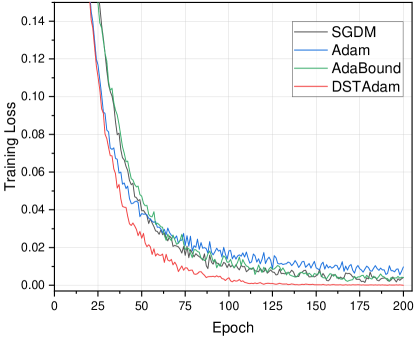
(a) Training loss

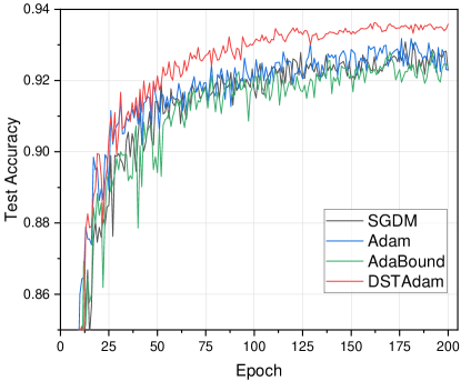
(b) Test accuracy

Figure 2: Training loss and test accuracy for ResNet-18 on CIFAR-10.

Results on CIFAR-10 dataset. We firstly test the performance of the proposed DSTAdam on the CIFAR-10 dataset, which consists of 60,000 32$\displaystyle\times$32 RGB color images drawn from 10 categories. Each category contains 5,000 training samples and 1,000 test samples. The training loss and the test accuracy of the four methods versus the number of epochs are plotted in Figure 2. From subfigure 2(a), we see that DSTAdam has faster convergence speed and lower steady-state loss than other algorithms. Figure 2(b) shows that the test accuracy of DSTAdam is also better than other algorithms, with an improvement of about 1% at the end of training. In addition, the loss and accuracy curves of DSTAdam are more smooth and stable, which reflect the effect of the decreasing scaling transition.

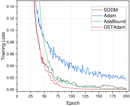
(a) Training loss

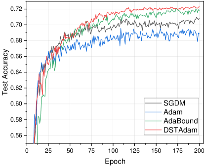
(b) Test accuracy

Figure 3: Training loss and test accuracy for ResNet-18 on CIFAR-100.

Results on CIFAR-100 dataset. We next perform experiments on the CIFAR-100 dataset, which contains 60,000 32$\displaystyle\times$32 color images in 100 classes. Each class has 500 training images and 100 test images. We plot the training loss and test accuracy of different methods with the same initialization in Figure 3. From the results, we observe that DSTAdam decreases the training loss faster and smoother than other methods, followed by SGDM and AdaBound, and that Adam is the slowest after the 50th epoch. For the test part, we find that DSTAdam performs slightly better than AdaBound but outperforms SGDM and Adam.

6 Conclusion

In this paper, we have presented a new transition method called DSTAdam, which achieves a smooth and stable transition from Adam to SGD through scaling operation instead of clipping operation. Our work extends the research which focus from the bound functions of the AdaBound to the transition operation, provideing a new perspective to understand AdaBound. Moreover, we have established the $\displaystyle\mathcal{O}({\sqrt{T}})$ regret bound of the proposed DSTAdam in the online convex setting. Finally, numerical experiments verify the effectiveness of DSTAdam on the CIFAR-10/100 datasets. The example results fully show that DSTAdam has fast convergence speed and good generalization performance, which reflect the advantages of Adam and SGD.

Appendices

Appendix A Proof of Theorem 4.1

We firstly provide the following lemmas for the proof of Theorem 4.1.

Lemma A.1

[16, 26] Let $\displaystyle a_{i}\geq 0,i=1,2\cdots,n$. Then

$$\sum\limits_{i=1}^{n}{\frac{{{a_{i}}}}{{\sqrt{\sum\limits_{j=1}^{i}{{a_{j}}}}}}}\leq 2\sqrt{\sum\limits_{i=1}^{n}{{a_{i}}}}.$$ (A.1)

Lemma A.2

[16, 27] For any $\displaystyle Q\in\mathcal{S}_{+}^{d}$ and convex feasible set $\displaystyle\mathcal{F}\subset\mathbb{R}^{d}$, suppose $\displaystyle u_{1}=\mathop{\arg\min}_{x\in\mathcal{F}}\left\|Q^{1/2}\left(x-z_{1}\right)\right\|$ and $\displaystyle u_{2}=\mathop{\arg\min}_{x\in\mathcal{F}}\left\|Q^{1/2}\left(x-z_{2}\right)\right\|$, then $\displaystyle\left\|{{Q^{1/2}}\left({{u_{1}}-{u_{2}}}\right)}\right\|\leq\left\|{{Q^{1/2}}\left({{z_{1}}-{z_{2}}}\right)}\right\|$.

Lemma A.3

Suppose that the conditions and parameter setting in Theorem 4.1 are satisfied, then we have

$$\sum\limits_{t=1}^{T}{\frac{1}{{\sqrt{t}}}{{\left\|{\hat{\eta}_{t}^{1/2}{m_{t}}}\right\|}^{2}}}\leq\frac{{2\alpha\rho\zeta}}{{{{\left({1-{\beta_{1}}}\right)}^{2}}}}\sum\limits_{i=1}^{d}{{{\left\|{{g_{1:T,i}}}\right\|}_{2}}}+\frac{{{r_{u}}\sqrt{1+\log T}}}{{{{\left({1-{\beta_{1}}}\right)}^{2}}}}\sum\limits_{i=1}^{d}{{{\left\|{g_{1:T,i}^{2}}\right\|}_{2}}}.$$

Proof 1

Recall the step 6 in Algorithm 2, we firstly have

$$\begin{split}\sum\limits_{t=1}^{T}{\frac{1}{{\sqrt{t}}}{{\left\|{\hat{\eta}_{t}^{1/2}{m_{t}}}\right\|}^{2}}}&=\sum\limits_{t=1}^{T-1}{\frac{1}{{\sqrt{t}}}{{\left\|{\hat{\eta}_{t}^{1/2}{m_{t}}}\right\|}^{2}}}+\frac{1}{{\sqrt{T}}}\sum\limits_{i=1}^{d}{m_{T,i}^{2}{{\hat{\eta}}_{T,i}}}\\ &=\sum\limits_{t=1}^{T-1}{\frac{1}{{\sqrt{t}}}{{\left\|{\hat{\eta}_{t}^{1/2}{m_{t}}}\right\|}^{2}}}+\frac{1}{{\sqrt{T}}}\sum\limits_{i=1}^{d}{m_{T,i}^{2}\left({\left({\frac{\alpha}{\sqrt{v_{T,i}}}-{r_{T}}}\right){\rho_{T}}+{r_{T}}}\right)}\\ &\leq\sum\limits_{t=1}^{T-1}{\frac{1}{{\sqrt{t}}}{{\left\|{\hat{\eta}_{t}^{1/2}{m_{t}}}\right\|}^{2}}}+\frac{1}{{\sqrt{T}}}\sum\limits_{i=1}^{d}{m_{T,i}^{2}\left(\frac{\alpha{\rho_{T}}}{\sqrt{v_{T,i}}}+{r_{T}}\right)}.\end{split}$$ (A.2)

Furthermore, the second term in the right-hand side (RHS) of the above equality can be estimated as follows

$$\begin{split}&\frac{1}{{\sqrt{T}}}\sum\limits_{i=1}^{d}m_{T,i}^{2}\left(\frac{\alpha{\rho_{T}}}{\sqrt{v_{T,i}}}+{r_{T}}\right)\\ &\leq\frac{1}{{\sqrt{T}}}\sum\limits_{i=1}^{d}{{{\left({\sum\limits_{j=1}^{T}{\prod\limits_{k=1}^{T-j}{{\beta_{1({T-k+1})}}}}}\right)\left({\sum\limits_{j=1}^{T}{\prod\limits_{k=1}^{T-j}{{\beta_{1({T-k+1})}}g_{j,i}^{2}}}}\right)}\left(\frac{\alpha{\rho_{T}}}{\sqrt{v_{T,i}}}+{r_{T}}\right)}}\\ &\leq\frac{1}{{\sqrt{T}}}\sum\limits_{i=1}^{d}{{\left({\sum\limits_{j=1}^{T}{\beta_{1}^{T-j}}}\right)\left({\sum\limits_{j=1}^{T}{\beta_{1}^{T-j}g_{j,i}^{2}}}\right)\left(\frac{\alpha{\rho_{T}}}{\sqrt{v_{T,i}}}+{r_{T}}\right)}}\\ &\leq\frac{\alpha{\rho_{T}}}{(1-\beta_{1}){\sqrt{T}}}\sum\limits_{i=1}^{d}{{\left({\sum\limits_{j=1}^{T}{\beta_{1}^{T-j}g_{j,i}^{2}}}\right)\frac{1}{\sqrt{v_{T,i}}}}}+\frac{{r_{T}}}{(1-\beta_{1}){\sqrt{T}}}\sum\limits_{i=1}^{d}{{\left({\sum\limits_{j=1}^{T}{\beta_{1}^{T-j}g_{j,i}^{2}}}\right)}}.\end{split}$$ (A.3)

By condition (C1) in Theorem 4.1, the first term in the RHS of the above inequality can be further simplified as

$$\begin{split}\frac{\alpha{\rho_{T}}}{(1-\beta_{1}){\sqrt{T}}}\sum\limits_{i=1}^{d}{{\left({\sum\limits_{j=1}^{T}{\beta_{1}^{T-j}g_{j,i}^{2}}}\right)\frac{1}{\sqrt{v_{T,i}}}}}&\leq\frac{\alpha{\rho_{T}}}{(1-\beta_{1})}\sum\limits_{i=1}^{d}{{\left({\sum\limits_{j=1}^{T}{\beta_{1}^{T-j}g_{j,i}^{2}}}\right)}}{\frac{1}{\frac{1}{\zeta}{\sqrt{\sum\limits_{j=1}^{T}{g_{j,i}^{2}}}}}}\\ &\leq\frac{{\alpha{\rho_{T}}\zeta}}{{\left({1-{\beta_{1}}}\right)}}\sum\limits_{i=1}^{d}{{\sum\limits_{j=1}^{T}{\frac{{\beta_{1}^{T-j}g_{j,i}^{2}}}{{\sqrt{\sum\limits_{k=1}^{j}{g_{k,i}^{2}}}}}}}}.\end{split}$$ (A.4)

Combining the above estimates, we arrive at

$$\begin{split}\sum\limits_{t=1}^{T}{\frac{1}{{\sqrt{t}}}{{\left\|{\hat{\eta}_{t}^{1/2}{m_{t}}}\right\|}^{2}}}&\leq\sum\limits_{t=1}^{T-1}{\frac{1}{{\sqrt{t}}}{{\left\|{\hat{\eta}_{t}^{1/2}{m_{t}}}\right\|}^{2}}}\\ &\quad+\frac{{\alpha{\rho_{T}}\zeta}}{{\left({1-{\beta_{1}}}\right)}}\sum\limits_{i=1}^{d}{{\sum\limits_{j=1}^{T}{\frac{{\beta_{1}^{T-j}g_{j,i}^{2}}}{{\sqrt{\sum\limits_{k=1}^{j}{g_{k,i}^{2}}}}}}}}+\frac{{{r_{T}}}}{{\left({1-{\beta_{1}}}\right)\sqrt{T}}}\sum\limits_{i=1}^{d}{\sum\limits_{j=1}^{T}{\beta_{1}^{T-j}g_{j,i}^{2}}}.\end{split}$$ (A.5)

By the principle of mathematical induction and the double-sum trick, we have

$$\begin{split}\sum\limits_{t=1}^{T}{\frac{1}{{\sqrt{t}}}{{\left\|{\hat{\eta}_{t}^{1/2}{m_{t}}}\right\|}^{2}}}&\leq\sum\limits_{t=1}^{T}{\frac{{\alpha{\rho_{t}}\zeta}}{{\left({1-{\beta_{1}}}\right)}}\sum\limits_{i=1}^{d}{{\sum\limits_{j=1}^{t}{\frac{{\beta_{1}^{t-j}g_{j,i}^{2}}}{{\sqrt{\sum\limits_{k=1}^{j}{g_{k,i}^{2}}}}}}}}}+\sum\limits_{t=1}^{T}{\frac{{{r_{t}}}}{{\left({1-{\beta_{1}}}\right)\sqrt{t}}}\sum\limits_{i=1}^{d}{\sum\limits_{j=1}^{t}{\beta_{1}^{t-j}g_{j,i}^{2}}}}\\ &\leq\frac{{\alpha\rho\zeta}}{{\left({1-{\beta_{1}}}\right)}}\sum\limits_{i=1}^{d}{\sum\limits_{t=1}^{T}{\sum\limits_{j=1}^{t}{\frac{{\beta_{1}^{t-j}g_{j,i}^{2}}}{{\sqrt{\sum\limits_{k=1}^{j}{g_{k,i}^{2}}}}}}}}+\frac{{{r_{u}}}}{{\left({1-{\beta_{1}}}\right)}}\sum\limits_{i=1}^{d}{\sum\limits_{t=1}^{T}{\frac{{\rm{1}}}{{\sqrt{t}}}}\sum\limits_{j=1}^{t}{\beta_{1}^{t-j}}g_{j,i}^{2}}\\ &=\frac{{\alpha\rho\zeta}}{{\left({1-{\beta_{1}}}\right)}}\sum\limits_{i=1}^{d}{\sum\limits_{t=1}^{T}{\frac{{g_{t,i}^{2}}}{{\sqrt{\sum\limits_{k=1}^{t}{g_{k,i}^{2}}}}}\sum\limits_{j=t}^{T}{\beta_{1}^{j-t}}}}+\frac{{{r_{u}}}}{{\left({1-{\beta_{1}}}\right)}}\sum\limits_{i=1}^{d}{\sum\limits_{t=1}^{T}{g_{t,i}^{2}}\sum\limits_{j=t}^{T}{\frac{{\beta_{1}^{j-t}}}{{\sqrt{j}}}}}\\ &\leq\frac{{\alpha\rho\zeta}}{{{{\left({1-{\beta_{1}}}\right)}^{2}}}}\sum\limits_{i=1}^{d}{\sum\limits_{t=1}^{T}{\frac{{g_{t,i}^{2}}}{{\sqrt{\sum\limits_{k=1}^{t}{g_{k,i}^{2}}}}}}}+\frac{{{r_{u}}}}{{\left({1-{\beta_{1}}}\right)^{2}}}\sum\limits_{i=1}^{d}{\sum\limits_{t=1}^{T}\frac{g_{t,i}^{2}}{{\sqrt{t}}}}.\end{split}$$ (A.6)

Upon applying Lemma A.1 and using Cauchy-Schwarz inequality, we obtain

$$\begin{split}\sum\limits_{t=1}^{T}{\frac{1}{{\sqrt{t}}}{{\left\|{\hat{\eta}_{t}^{1/2}{m_{t}}}\right\|}^{2}}}&\leq\frac{{\alpha\rho\zeta}}{{{{\left({1-{\beta_{1}}}\right)}^{2}}}}\sum\limits_{i=1}^{d}{2\sqrt{\sum\limits_{t=1}^{T}{g_{t,i}^{2}}}}+\frac{{{r_{u}}}}{{{{\left({1-{\beta_{1}}}\right)}^{2}}}}\sum\limits_{i=1}^{d}{{{\left\|{g_{1:T,i}^{2}}\right\|}_{2}}\sqrt{\sum\limits_{t=1}^{T}{\frac{1}{t}}}}\\ &\leq\frac{{2\alpha\rho\zeta}}{{{{\left({1-{\beta_{1}}}\right)}^{2}}}}\sum\limits_{i=1}^{d}{{{\left\|{{g_{1:T,i}}}\right\|}_{2}}}+\frac{{{r_{u}}\sqrt{1+\log T}}}{{{{\left({1-{\beta_{1}}}\right)}^{2}}}}\sum\limits_{i=1}^{d}{{{\left\|{g_{1:T,i}^{2}}\right\|}_{2}}}.\end{split}$$ (A.7)

Now we are ready to prove Theorem 4.1.

Proof of Theorem 1. By the definition of projection, we have

$$\begin{split}{\theta_{t+1}}={\Pi_{{\rm{{\cal F}}},{\hat{\eta}_{t}^{-1}}}}\left({{\theta_{t}}-\frac{1}{{\sqrt{t}}}{{\hat{\eta}}_{t}}{m_{t}}}\right)=\mathop{\mathop{\arg\min}}\limits_{\theta\in{\rm{{\cal F}}}}\left\|{\hat{\eta}_{t}^{-1/2}\left({\theta-\left({{\theta_{t}}-\frac{1}{{\sqrt{t}}}{{\hat{\eta}}_{t}}{m_{t}}}\right)}\right)}\right\|.\end{split}$$ (A.8)

Note that $\displaystyle\Pi_{\mathcal{F},\hat{\eta}_{t}^{-1}}\left({\theta^{*}}\right)={\theta^{*}}$ for all $\displaystyle\theta^{*}\in\mathcal{F}$. Using Lemma A.2 with $\displaystyle{u_{1}}={\theta_{t+1}}$ and $\displaystyle{u_{2}}={\theta^{*}}$, we have

$$\begin{split}{\left\|{\hat{\eta}_{t}^{-1/2}\left({{\theta_{t+1}}-{\theta^{*}}}\right)}\right\|^{2}}&\leq{\left\|{\hat{\eta}_{t}^{-1/2}\left({{\theta_{t}}-\frac{1}{{\sqrt{t}}}{{\hat{\eta}}_{t}}{m_{t}}-{\theta^{*}}}\right)}\right\|^{2}}\\ &={\left\|{\hat{\eta}_{t}^{-1/2}\left({{\theta_{t}}-{\theta^{*}}}\right)}\right\|^{2}}+\frac{1}{t}{\left\|{\hat{\eta}_{t}^{1/2}{m_{t}}}\right\|^{2}}-\frac{2}{{\sqrt{t}}}\left\langle{{\beta_{1t}}{m_{t-1}}+\left({1-{\beta_{1t}}}\right){g_{t}},{\theta_{t}}-{\theta^{*}}}\right\rangle.\end{split}$$ (A.9)

Rearranging the terms in the above inequality, we have

$$\begin{split}&\left\langle g_{t},\theta_{t}-\theta^{*}\right\rangle\\ &\leq\frac{\sqrt{t}}{2\left(1-\beta_{1t}\right)}\left[\left\|\hat{\eta}_{t}^{-1/2}\left(\theta_{t}-\theta^{*}\right)\right\|^{2}-\left\|\hat{\eta}_{t}^{-1/2}\left(\theta_{t+1}-\theta^{*}\right)\right\|^{2}\right]\\ &\quad+\frac{1}{2\sqrt{t}\left(1-\beta_{1t}\right)}\left\|\hat{\eta}_{t}^{1/2}m_{t}\right\|^{2}-\frac{\beta_{1t}}{\left(1-\beta_{1t}\right)}\left\langle m_{t-1},\theta_{t}-\theta^{*}\right\rangle\\ &\leq\frac{\sqrt{t}}{2\left(1-\beta_{1t}\right)}\left[\left\|\hat{\eta}_{t}^{-1/2}\left(\theta_{t}-\theta^{*}\right)\right\|^{2}-\left\|\hat{\eta}_{t}^{-1/2}\left(\theta_{t+1}-\theta^{*}\right)\right\|^{2}\right]+\frac{1}{2\sqrt{t}\left(1-\beta_{1t}\right)}\left\|\hat{\eta}_{t}^{1/2}m_{t}\right\|^{2}\\ &\quad+\frac{\beta_{1t}\sqrt{t}}{2\left(1-\beta_{1t}\right)}\left\|\hat{\eta}_{t}^{-1/2}\left(\theta_{t}-\theta^{*}\right)\right\|^{2}+\frac{\beta_{1t}}{2\sqrt{t}\left(1-\beta_{1t}\right)}\left\|\hat{\eta}_{t}^{1/2}m_{t-1}\right\|^{2},\end{split}$$ (A.10)

where the last inequality follows from a basic inequality $\displaystyle xy\leq\frac{\kappa x^{2}}{2}+\frac{y^{2}}{2\kappa},\kappa>0$. By the convexity of function $\displaystyle{f_{t}}$ and the above inequality, we arrive at

$$\begin{split}&\sum\limits_{t=1}^{T}{\left({{f_{t}}\left({{\theta_{t}}}\right)-{f_{t}}\left({{\theta^{*}}}\right)}\right)}\leq\sum\limits_{t=1}^{T}\left\langle g_{t},\theta_{t}-\theta^{*}\right\rangle\\ &\leq\sum\limits_{t=1}^{T}{\frac{{\sqrt{t}}}{{2\left({1-{\beta_{1}}}\right)}}\left[{{{\|{\hat{\eta}_{t}^{-1/2}\left({{\theta_{t}}-{\theta^{*}}}\right)}\|}^{2}}\!-\!{{\|{\hat{\eta}_{t}^{-1/2}\left({{\theta_{t+1}}-{\theta^{*}}}\right)}\|}^{2}}}\right]}\!+\!\sum\limits_{t=1}^{T}{\frac{{{\beta_{1t}}\sqrt{t}}}{{2\left({1-{\beta_{1t}}}\right)}}{{\left\|{\hat{\eta}_{t}^{-1/2}\left({{\theta_{t}}-{\theta^{*}}}\right)}\right\|}^{2}}}\\ &\quad+\sum\limits_{t=1}^{T}{\frac{1}{{2\sqrt{t}\left({1-{\beta_{1}}}\right)}}{{\left\|{\hat{\eta}_{t}^{1/2}{m_{t}}}\right\|}^{2}}}+\sum\limits_{t=1}^{T-1}{\frac{{{\beta_{1}}}}{{2\sqrt{t+1}\left({1-{\beta_{1}}}\right)}}{{\left\|{\hat{\eta}_{t+1}^{1/2}{m_{t}}}\right\|}^{2}}}.\end{split}$$ (A.11)

By the conditions (C2) and $\displaystyle\left\|x-y\right\|_{\infty}\leq D_{\infty}$, $\displaystyle\forall x,y\in\mathcal{F}$. Then, the first term in the RHS of (A.11) can be estimated as

$$\begin{split}&\sum_{t=1}^{T}\frac{\sqrt{t}}{2\left(1-\beta_{1t}\right)}\left[\left\|\hat{\eta}_{t}^{-1/2}\left(\theta_{t}-\theta^{*}\right)\right\|^{2}-\left\|\hat{\eta}_{t}^{-1/2}\left(\theta_{t+1}-\theta^{*}\right)\right\|^{2}\right]\\ &\leq\frac{\left\|\hat{\eta}_{1}^{-1/2}\left(\theta_{1}-\theta^{*}\right)\right\|}{2\left(1-\beta_{1}\right)}+\sum_{t=2}^{T}\frac{\sqrt{t}}{2\left(1-\beta_{1t}\right)}\left[\left\|\hat{\eta}^{-1/2}\left(\theta_{t}-\theta^{*}\right)\right\|^{2}-\left\|\hat{\eta}_{t-1}^{-1/2}\left(\theta_{t}-\theta^{*}\right)\right\|^{2}\right]\\ &\leq\frac{\left\|\hat{\eta}_{1}^{-1/2}\right\|}{2\left(1-\beta_{1}\right)}D_{\infty}^{2}+\frac{1}{2\left(1-\beta_{1}\right)}\sum_{t=2}^{T}\left(\sqrt{t}\left\|\hat{\eta}_{t}^{-1/2}D_{\infty}\right\|^{2}-\sqrt{t-1}\left\|\hat{\eta}_{t-1}^{-1/2}D_{\infty}\right\|^{2}\right)\\ &=\frac{\sqrt{T}D_{\infty}^{2}\left\|\hat{\eta}_{T}^{-1/2}\right\|^{2}}{2\left(1-\beta_{1}\right)}.\end{split}$$ (A.12)

By condition (C2) in Theorem 4.1, the last term in the RHS of (A.11) can be simplified as

$$\begin{split}\sum\limits_{t=1}^{T-1}{\frac{{{\beta_{1}}}}{{2\sqrt{t+1}\left({1-{\beta_{1}}}\right)}}{{\left\|{\hat{\eta}_{t+1}^{1/2}{m_{t}}}\right\|}^{2}}}\leq\sum\limits_{t=1}^{T}{\frac{1}{{2\sqrt{t}\left({1-{\beta_{1}}}\right)}}{{\left\|{\hat{\eta}_{t}^{1/2}{m_{t}}}\right\|}^{2}}}.\end{split}$$ (A.13)

Summarizing the above estimates and applying Lemma A.3, we obtain

$$\begin{split}\sum\limits_{t=1}^{T}{\left({{f_{t}}\left({{\theta_{t}}}\right)-{f_{t}}\left({{\theta^{*}}}\right)}\right)}&\leq\frac{\sqrt{T}D_{\infty}^{2}\left\|\hat{\eta}_{T}^{-1/2}\right\|^{2}}{2\left(1-\beta_{1}\right)}+\sum\limits_{t=1}^{T}{\frac{{{\beta_{1t}}\sqrt{t}}}{{2\left({1-{\beta_{1t}}}\right)}}{{\left\|{\hat{\eta}_{t}^{-1/2}\left({{\theta_{t}}-{\theta^{*}}}\right)}\right\|}^{2}}}\\ &\quad+\frac{{2\alpha\rho\zeta}}{{{{\left({1-{\beta_{1}}}\right)}^{3}}}}\sum\limits_{i=1}^{d}{{{\left\|{{g_{1:T,i}}}\right\|}_{2}}}+\frac{{{r_{u}}\sqrt{1+\log T}}}{{{{\left({1-{\beta_{1}}}\right)}^{3}}}}\sum\limits_{i=1}^{d}{{{\left\|{g_{1:T,i}^{2}}\right\|}_{2}}}\\ &\leq\frac{\sqrt{T}D_{\infty}^{2}}{2\left(1-\beta_{1}\right)}\sum_{i=1}^{d}\hat{\eta}_{T,i}^{-1}+\frac{D_{\infty}^{2}}{2\left(1-\beta_{1}\right)}\sum_{t=1}^{T}\sum_{i=1}^{d}\frac{\beta_{1t}\sqrt{t}}{\hat{\eta}_{t,i}}\\ &\quad+\frac{2\alpha\rho\zeta}{\left(1-\beta_{1}\right)^{3}}\sum_{i=1}^{d}\left\|g_{1:T,i}\right\|_{2}+\frac{r_{u}\sqrt{1+\log T}}{\left(1-\beta_{1}\right)^{3}}\sum_{i=1}^{d}\left\|g_{1:T,i}^{2}\right\|_{2}.\end{split}$$ (A.14)

We proceed to prove Corollary 4.1 and Corollary 4.2 from Theorem 4.1.

Proof of Corollary 1. Recall the step 6 in Algorithm 2, we have

$$\begin{split}\hat{\eta}_{t,i}^{-1}&=\left(\rho_{t}\left(\frac{\alpha}{\sqrt{v_{t,i}}}-r_{t}\right)+r_{t}\right)^{-1}\\ &=\frac{1}{\frac{\alpha\rho_{t}}{\sqrt{v_{t,i}}}-r_{t}\rho_{t}+r_{t}}\\ &\leq\frac{1}{r_{t}-r_{t}\rho_{t}}\\ &\leq\frac{1}{r_{l}(1-\rho)}.\end{split}$$ (A.15)

Since $\displaystyle{\beta_{1t}}={\beta_{1}}{\lambda^{t-1}}$, it follows that

$$\begin{split}\sum_{t=1}^{T}\sum_{i=1}^{d}\frac{\beta_{1t}\sqrt{t}}{\hat{\eta}_{t,i}}&\leq\frac{\beta_{1}d}{r_{l}(1-\rho)}\sum_{t=1}^{T}\lambda^{t-1}\sqrt{t}\\ &\leq\frac{d}{r_{l}(1-\rho)}\sum_{t=1}^{T}\lambda^{t-1}t\\ &=\frac{d}{r_{l}(1-\rho)}\left(\frac{1-\lambda^{T}}{(1-\lambda)^{2}}-\frac{\lambda^{T}T}{(1-\lambda)}\right)\\ &\leq\frac{d}{r_{l}(1-\rho)(1-\lambda)^{2}}.\end{split}$$ (A.16)

Based on the result in Theorem 4.1, we obtain

$$\begin{split}R(T)&\leq\frac{\sqrt{T}D_{\infty}^{2}}{2\left(1-\beta_{1}\right)}\sum_{i=1}^{d}\hat{\eta}_{T,i}^{-1}+\frac{dD_{\infty}^{2}}{2r_{l}(1-\rho)(1-\lambda)^{2}\left(1-\beta_{1}\right)}\\ &\quad+\frac{2\alpha\rho\zeta}{\left(1-\beta_{1}\right)^{3}}\sum_{i=1}^{d}\left\|g_{1:T,i}\right\|_{2}+\frac{r_{u}\sqrt{1+\log T}}{\left(1-\beta_{1}\right)^{3}}\sum_{i=1}^{d}\left\|g_{1:T,i}^{2}\right\|_{2}.\end{split}$$ (A.17)

Proof of Corollary 2. Since $\displaystyle{\beta_{1t}}={\beta_{1}}/t$, it follows that

$$\begin{split}\sum_{t=1}^{T}\sum_{i=1}^{d}\frac{\beta_{1t}\sqrt{t}}{\hat{\eta}_{t,i}}&\leq\frac{\beta_{1}d}{r_{l}(1-\rho)}\sum_{t=1}^{T}\frac{\sqrt{t}}{t}\\ &\leq\frac{d}{r_{l}(1-\rho)}\sum_{t=1}^{T}2(\sqrt{t}-\sqrt{t-1})\\ &\leq\frac{2d\sqrt{T}}{r_{l}(1-\rho)}.\end{split}$$ (A.18)

Based on the result in Theorem 4.1, we obtain

$$\begin{split}R(T)&\leq\frac{\sqrt{T}D_{\infty}^{2}}{2\left(1-\beta_{1}\right)}\sum_{i=1}^{d}\hat{\eta}_{T,i}^{-1}+\frac{dD_{\infty}^{2}\sqrt{T}}{r_{l}(1-\rho)\left(1-\beta_{1}\right)}\\ &\quad+\frac{2\alpha\rho\zeta}{\left(1-\beta_{1}\right)^{3}}\sum_{i=1}^{d}\left\|g_{1:T,i}\right\|_{2}+\frac{r_{u}\sqrt{1+\log T}}{\left(1-\beta_{1}\right)^{3}}\sum_{i=1}^{d}\left\|g_{1:T,i}^{2}\right\|_{2}.\end{split}$$ (A.19)

References

- Krizhevsky et al. [2012] A. Krizhevsky, I. Sutskever, G. E. Hinton, Imagenet classification with deep convolutional neural networks, in: Advances in Neural Information Processing Systems, 2012, pp. 1097–1105.
- Wu et al. [2016] Y. Wu, M. Schuster, Z. Chen, Q. V. Le, M. Norouzi, W. Macherey, M. Krikun, Y. Cao, Q. Gao, K. Macherey, et al., Google’s neural machine translation system: Bridging the gap between human and machine translation, arXiv preprint arXiv:1609.08144 (2016).
- Azghadi et al. [2020] M. R. Azghadi, C. Lammie, J. K. Eshraghian, M. Payvand, E. Donati, B. Linares-Barranco, G. Indiveri, Hardware implementation of deep network accelerators towards healthcare and biomedical applications, IEEE Transactions on Biomedical Circuits and Systems 14 (2020) 1138–1159.
- Kato et al. [2016] N. Kato, Z. M. Fadlullah, B. Mao, F. Tang, O. Akashi, T. Inoue, K. Mizutani, The deep learning vision for heterogeneous network traffic control: Proposal, challenges, and future perspective, IEEE wireless communications 24 (2016) 146–153.
- Rumelhart et al. [1986] D. E. Rumelhart, G. E. Hinton, R. J. Williams, Learning representations by back-propagating errors, Nature 323 (1986) 533–536.
- LeCun et al. [1989] Y. LeCun, B. Boser, J. Denker, D. Henderson, R. Howard, W. Hubbard, L. Jackel, Handwritten digit recognition with a back-propagation network, in: Advances in neural information processing systems, 1989, p. 396–404.
- Hochreiter and Schmidhuber [1997] S. Hochreiter, J. Schmidhuber, Long short-term memory, Neural computation 9 (1997) 1735–1780.
- He et al. [2016] K. He, X. Zhang, S. Ren, J. Sun, Deep residual learning for image recognition, in: Proceedings of the IEEE conference on computer vision and pattern recognition, 2016, pp. 770–778.
- Huang et al. [2017] G. Huang, Z. Liu, L. Van Der Maaten, K. Q. Weinberger, Densely connected convolutional networks, in: Proceedings of the IEEE conference on computer vision and pattern recognition, 2017, pp. 4700–4708.
- Robbins and Monro [1951] H. Robbins, S. Monro, A stochastic approximation method, Annals of Mathematical Statistics 22 (1951) 400–407.
- Polyak [1964] B. T. Polyak, Some methods of speeding up the convergence of iteration methods, Ussr computational mathematics and mathematical physics 4 (1964) 1–17.
- Duchi et al. [2011] J. Duchi, E. Hazan, Y. Singer, Adaptive subgradient methods for online learning and stochastic optimization, Journal of machine learning research 12 (2011) 2121–2159.
- Hinton et al. [2012] G. Hinton, N. Srivastava, K. Swersky, T. Tieleman, A. Mohamed, Coursera: Neural networks for machine learning, Lecture 9c: Using noise as a regularizer (2012).
- Zeiler [2012] M. D. Zeiler, Adadelta: An adaptive learning rate method, arXiv preprint arXiv:1212.5701 (2012).
- Kingma and Ba [2015] D. P. Kingma, J. Ba, Adam: A method for stochastic optimization, in: 3rd International Conference on Learning Representations, 2015.
- Reddi et al. [2018] S. J. Reddi, S. Kale, S. Kumar, On the convergence of Adam and beyond, in: 6th International Conference on Learning Representations, 2018.
- Keskar and Socher [2017] N. S. Keskar, R. Socher, Improving generalization performance by switching from Adam to SGD, arXiv preprint arXiv:1712.07628 (2017).
- Luo et al. [2019] L. Luo, Y. Xiong, Y. Liu, X. Sun, Adaptive gradient methods with dynamic bound of learning rate, in: 7th International Conference on Learning Representations, 2019.
- Liang et al. [2020] D. Liang, F. Ma, W. Li, New gradient-weighted adaptive gradient methods with dynamic constraints, IEEE Access 8 (2020) 110929–110942.
- Yang and Cai [2021] L. Yang, D. Cai, AdaDB: An adaptive gradient method with data-dependent bound, Neurocomputing 419 (2021) 183–189.
- Lu et al. [2020] Z. Lu, M. Lu, Y. Liang, A distributed neural network training method based on hybrid gradient computing, Scalable Computing: Practice and Experience 21 (2020) 323–336.
- Zinkevich [2003] M. Zinkevich, Online convex programming and generalized infinitesimal gradient ascent, in: Proceedings of the 20th international conference on machine learning, 2003, pp. 928–936.
- Zhou et al. [2019] Z. Zhou, Q. Zhang, G. Lu, H. Wang, W. Zhang, Y. Yu, AdaShift: Decorrelation and convergence of adaptive learning rate methods, in: 7th International Conference on Learning Representations, 2019.
- Bock et al. [2018] S. Bock, J. Goppold, M. Weiß, An improvement of the convergence proof of the ADAM-optimizer, arXiv preprint arXiv:1804.10587 (2018).
- Krizhevsky and Hinton [2009] A. Krizhevsky, G. Hinton, Learning multiple layers of features from tiny images, Master’s thesis, Department of Computer Science, University of Toronto (2009).
- Auer et al. [2002] P. Auer, N. Cesa-Bianchi, C. Gentile, Adaptive and self-confident on-line learning algorithms, Journal of Computer & System Sciences 64 (2002) 48–75.
- Mcmahan and Streeter [2010] H. B. Mcmahan, M. Streeter, Adaptive bound optimization for online convex optimization, Computer Science 7 (2010) 163–71.