Singularity of energy measures on a class of inhomogeneous Sierpinski gaskets

Abstract.

We study energy measures of canonical Dirichlet forms on inhomogeneous Sierpinski gaskets. We prove that the energy measures and suitable reference measures are mutually singular under mild assumptions.

This study was supported by JSPS KAKENHI Grant Numbers JP19H00643 and JP19K21833.

1 Introduction

Energy measures associated with regular Dirichlet forms are fundamental concepts in stochastic analysis and related fields. For example, the intrinsic metric is defined by using energy measures and appears in Gaussian estimates of the transition probabilities. Energy measures are also crucial for describing the conditions for sub-Gaussian behaviors of transition densities. The energy measures are expected to be singular with respect to (canonical) underlying measures for canonical Dirichlet forms on self-similar fractals, which has been confirmed in many cases [13, 4, 9, 10]. Recently, such a singularity was proved under full off-diagonal sub-Gaussian estimates of the transition densities [11].

In this paper, we study a class of inhomogeneous Sierpinski gaskets as examples that have not yet been covered in the previous studies: they do not necessarily have strict self-similar structures or nice sub-Gaussian estimates. We show that the singularity of the energy measures still holds under mild assumptions. The strategy of our proof is based on quantitative estimates of probability measures on shift spaces, the techniques of which were used in [9, 10]. We expect this study to lead to further progress in stochastic analysis of complicated spaces of this kind.

This paper is organized as follows: In Section 2, we introduce a class of inhomogeneous Sierpinski gaskets and canonical Dirichlet forms defined on them, and state the main results. In Sections 3 and 4, we provide preliminary lemmas and prove the theorems. In Section 5, we make some concluding remarks.

2 Framework and statement of theorems

We begin by recalling $2$-dimensional level-$\nu$ Sierpinski gaskets $\mathrm{SG}(\nu)$ for $\nu\geq 2$. Let $N(\nu)=\nu(\nu+1)/2$. Let $\tilde{K}$ be an equilateral triangle in ${\mathbb{R}}^{2}$ including the interior. Let $K_{i}^{(\nu)}\subset\tilde{K}$, $i=1,2,\dots,N(\nu)$, be equilateral triangles including the interior that are obtained by dividing the sides of $\tilde{K}$ in $\nu$, joining these points, and removing all the downward-pointing triangles, as in Figure 1.

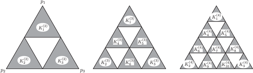
Figure 1: $K_{i}^{(\nu)}$, the image of $\tilde{K}$ by the contractive affine map $\psi_{i}^{(\nu)}$ $(\nu=2,3,4)$.

Let $\psi_{i}^{(\nu)}$, $i=1,2,\dots,N(\nu)$, be the contractive affine map from $\tilde{K}$ onto $K_{i}^{(\nu)}$ of type $\psi_{i}^{(\nu)}(z)=\nu^{-1}z+\alpha_{i}^{(\nu)}$ for some $\alpha_{i}^{(\nu)}\in{\mathbb{R}}^{2}$. Then, the $2$-dimensional level-$\nu$ Sierpinski gasket $\mathrm{SG}(\nu)$ is defined as a unique non-empty compact subset $K$ in $\tilde{K}$ such that

$$K=\bigcup_{i=1}^{N(\nu)}\psi_{i}^{(\nu)}(K).$$

Let $S_{0}=\{1,2,3\}$, and let $V_{0}=\{p_{1},p_{2},p_{3}\}$ be the set of all vertices of $\tilde{K}$. In the definition of $\mathrm{SG}(\nu)$, the labeling of $K_{i}^{(\nu)}$ does not matter. For later convenience, we assign $K_{i}^{(\nu)}$ for $i\in S_{0}$ to the triangle that contains $p_{i}$. As a result, $\psi_{i}^{(\nu)}$ has a fixed point $p_{i}$.

For a general non-empty set $X$, denote by $l(X)$ the set of all real-valued functions on $X$. When $X$ is finite, the inner product $(\cdot,\cdot)$ on $l(X)$ is defined by

$$(x,y)=\sum_{p\in X}x(p)y(p),\quad x,y\in l(X).$$

We regard $l(X)$ as the $L^{2}$-space on $X$ equipped with the counting measure. Then, the $L^{2}$-inner product is identical with $(\cdot,\cdot)$. The induced norm is denoted by $|\mathrel{\cdot}|$.

A symmetric linear operator $D=(D_{p,q})_{p,q\in V_{0}}$ on $l(V_{0})$ is defined as

$$D_{p,q}=\begin{cases}-2&\text{if }p=q,\\ 1&\text{otherwise}.\end{cases}$$

Let

$$Q(x,y):=(-Dx,y)=-\sum_{p,q\in V_{0}}D_{p,q}x(q)y(p)$$

for $x,y\in l(V_{0})$. More explicitly,

$$Q(x,y) =(x(p_{1})-x(p_{2}))(y(p_{1})-y(p_{2}))+(x(p_{2})-x(p_{3}))(y(p_{2})-y(p_{3}))$$

$$\quad+(x(p_{3})-x(p_{1}))(y(p_{3})-y(p_{1})).$$

This is a Dirichlet form on $l(V_{0})$. To simplify the notation, we sometimes write $Q(x)$ for $Q(x,x)$.

Let

$$V_{1}^{(\nu)}=\bigcup_{i=1}^{N(\nu)}\psi_{i}^{(\nu)}(V_{0}).$$

Let $r^{(\nu)}>0$ and $Q^{(\nu)}$ be a symmetric bilinear form on $V_{1}^{(\nu)}$ that is defined by

$$Q^{(\nu)}(x,y)=\sum_{i=1}^{N(\nu)}\frac{1}{r^{(\nu)}}Q(x\circ\psi_{i}^{(\nu)}|_{V_{0}},y\circ\psi_{i}^{(\nu)}|_{V_{0}}),\quad x,y\in l(V_{1}^{(\nu)}).$$

Then, there exists a unique $r^{(\nu)}>0$ such that, for every $x\in l(V_{0})$,

$$Q(x,x)=\inf\bigl{\{}Q^{(\nu)}(y,y)\bigm{|}y\in l(V_{1}^{(\nu)})\text{ and }y|_{V_{0}}=x\bigr{\}}.$$ (2.1)

Hereafter, we fix such $r^{(\nu)}$. For example, $r^{(2)}=3/5$, $r^{(3)}=7/15$, and $r^{(4)}=41/103$, which are confirmed by the concrete calculation.

For each $x\in l(V_{0})$, there exists a unique $y\in l(V_{1})$ that attains the infimum in (2.1). For $i=1,2,\dots,N(\nu)$, the map $l(V_{0})\ni x\mapsto y\circ\psi_{i}^{(\nu)}|_{V_{0}}\in l(V_{0})$ is linear, which is denoted by $A_{i}^{(\nu)}$. Then, it holds that

$$Q(x,x)=\sum_{i=1}^{N(\nu)}\frac{1}{r^{(\nu)}}Q(A_{i}^{(\nu)}x,A_{i}^{(\nu)}x),\quad x\in l(V_{0}).$$ (2.2)

We can construct a Dirichlet form on $\mathrm{SG}(\nu)$ by using such data, but we omit the explanation because we discuss it in more general situations soon.

For reference, we give a quantitative estimate of $r^{(\nu)}$. definition

Lemma 2.1

$1/\nu<r^{(\nu)}<N(\nu)/\nu^{2}$.

Proof 2.2

This kind of inequality should be well-known (see, e.g., [2, Theorem 1]), and see the proof of [11, Proposition 5.3] (and also [1, Proposition 6.30]) for the second inequality. For the first inequality, let

$$\alpha=\inf\{Q(z,z)\mid z\in l(V_{0}),\ z(p_{1})=1,\ z(p_{2})=0\}>0.$$ (2.3)

Then, for general $z\in l(V_{0})$,

$$Q(z,z)\geq(z(p_{1})-z(p_{2}))^{2}\alpha$$ (2.4)

by considering $(z-z(p_{2}))/(z(p_{1})-z(p_{2}))$.

The infimum of (2.3) is attained by $x\in l(V_{0})$ given by $x(p_{1})=1$, $x(p_{2})=0$, $x(p_{3})=1/2$ (and $\alpha=3/2$). Take $y\in l(V_{1}^{(\nu)})$ attaining the infimum of (2.1). Let $I\subset\{1,2,\dots,N(\nu)\}$ be a $\nu$-points set such that, for each $i\in I$, the intersection of $\psi_{i}^{(\nu)}(V_{0})$ and the segment connecting $p_{1}$ and $p_{2}$ is a two-points set, say $\{\check{p}_{i},\hat{p}_{i}\}$. Note that $3\notin I$, and $y$ is not constant on $\psi_{3}^{(\nu)}(V_{0})$, which is confirmed by applying the maximum principle (see, e.g., [12, Proposition 2.1.7]) to the graph whose vertices are all points of $V_{1}^{(\nu)}$ included in the triangle with $p_{1}$, $p_{3}$ and the middle point of $p_{1}$ and $p_{2}$ as the three vertices. Therefore,

$$\alpha =Q^{(\nu)}(y,y)$$

$$>\sum_{i\in I}\frac{1}{r^{(\nu)}}Q(y\circ\psi_{i}^{(\nu)}|_{V_{0}},y\circ\psi_{i}^{(\nu)}|_{V_{0}})$$

$$\geq\frac{1}{r^{(\nu)}}\sum_{i\in I}(y(\check{p}_{i})-y(\hat{p}_{i}))^{2}\alpha\quad\text{(from \eqref{eq:lower})}$$

$$\geq\frac{\alpha}{r^{(\nu)}}\Biggl{(}\sum_{i\in I}(y(\check{p}_{i})-y(\hat{p}_{i}))\Biggr{)}^{2}\Biggl{(}\sum_{i\in I}1\Biggr{)}^{-1}$$

$$=\frac{\alpha}{r^{(\nu)}}\cdot 1\cdot\nu^{-1}.$$

Thus, $1/\nu<r^{(\nu)}$.

See also [8] for the asymptotic behavior of $r^{(\nu)}$ as $\nu\to\infty$.

We now introduce $2$-dimensional inhomogeneous Sierpinski gaskets. We fix a non-empty finite subset $T$ of $\{\nu\in{\mathbb{N}}\mid\nu\geq 2\}$. For each $\nu\in T$, let $S^{(\nu)}$ denote the set of the letters $i^{\nu}$ for $i=1,2,\dots,N(\nu)$. We set $S=\bigcup_{\nu\in T}S^{(\nu)}$ and $\Sigma=S^{\mathbb{N}}$. For example, if $T=\{2,3\}$, then

$$S^{(2)} =\{1^{2},2^{2},3^{2}\},\quad S^{(3)}=\{1^{3},2^{3},3^{3},4^{3},5^{3},6^{3}\},$$

and $S=S^{(2)}\cup S^{(3)}$ has nine elements. (Note that $i^{\nu}$ does not mean $\underbrace{ii\cdots i}_{\nu}$, the $\nu$-letter word consisting of only $i$, in this paper.)

For each $v\in S$, a shift operator $\sigma_{v}\colon\Sigma\to\Sigma$ is defined by $\sigma_{v}(\omega_{1}\omega_{2}\cdots)=v\omega_{1}\omega_{2}\cdots$. Let $W_{0}=\{\emptyset\}$ and $W_{m}=S^{m}$ for $m\in{\mathbb{N}}$, and define $W_{\leq n}=\bigcup_{m=0}^{n}W_{m}$ and $W_{*}=\bigcup_{m\in{\mathbb{Z}}_{+}}W_{m}$. Here, ${\mathbb{Z}}_{+}:={\mathbb{N}}\cup\{0\}$. For $w\in W_{m}$, $|w|$ represents $m$ and is called the length of $w$. For $w=w_{1}\cdots w_{m}\in W_{m}$ and $w^{\prime}=w^{\prime}_{1}\cdots w^{\prime}_{n}\in W_{n}$, $ww^{\prime}\in W_{m+n}$ denotes $w_{1}\cdots w_{m}w^{\prime}_{1}\cdots w^{\prime}_{n}$. Also, $\sigma_{w}\colon\Sigma\to\Sigma$ is defined as $\sigma_{w}=\sigma_{w_{1}}\circ\cdots\circ\sigma_{w_{m}}$, and let $\Sigma_{w}=\sigma_{w}(\Sigma)$. For $k\leq m$, $[w]_{k}$ denotes $w_{1}\cdots w_{k}\in W_{k}$. Similarly, for $\omega=\omega_{1}\omega_{2}\cdots\in\Sigma$ and $n\in{\mathbb{N}}$, let $[\omega]_{n}$ denote $\omega_{1}\cdots\omega_{n}\in W_{n}$. By convention, $\sigma_{\emptyset}\colon\Sigma\to\Sigma$ is the identity map, $[w]_{0}:=\emptyset\in W_{0}$ for $w\in W_{*}$, and $[\omega]_{0}:=\emptyset\in W_{0}$ for $\omega\in\Sigma$.

For $i^{\nu}\in S$, we define $\psi_{i^{\nu}}:=\psi_{i}^{(\nu)}$ and $A_{i^{\nu}}:=A_{i}^{(\nu)}$. For $w=w_{1}w_{2}\cdots w_{m}\in W_{m}$, $\psi_{w}$ denotes $\psi_{w_{1}}\circ\psi_{w_{2}}\circ\dots\circ\psi_{w_{m}}$ and $A_{w}$ denotes $A_{w_{m}}\cdots A_{w_{2}}A_{w_{1}}$. Here, $\psi_{\emptyset}$ and $A_{\emptyset}$ are the identity maps by definition. For $\omega\in\Sigma$, $\bigcap_{m\in{\mathbb{Z}}_{+}}\psi_{[\omega]_{m}}(\tilde{K})$ is a one-point set $\{p\}$. The map $\Sigma\ni\omega\mapsto p\in\tilde{K}$ is denoted by $\pi$. The relation $\psi_{v}\circ\pi=\pi\circ\sigma_{v}$ holds for $v\in S$.

Now, we fix $L=\{L_{w}\}_{w\in W_{*}}\in T^{W_{*}}$. That is, we assign each $w\in W_{*}$ to $L_{w}\in T$. We set $\tilde{W}_{0}=\{\emptyset\}$ and

$$\tilde{W}_{m}=\bigcup_{w\in\tilde{W}_{m-1}}\bigl{\{}wv\bigm{|}v\in S^{(L_{w})}\bigr{\}}$$

for $m\in{\mathbb{N}}$, inductively. Define $\tilde{W}_{*}=\bigcup_{m\in{\mathbb{Z}}_{+}}\tilde{W}_{m}\subset W_{*}$, $\tilde{\Sigma}=\{\omega\in\Sigma\mid[\omega]_{m}\in\tilde{W}_{m}\text{ for all }m\in{\mathbb{Z}}_{+}\}$ and $G(L)=\pi(\tilde{\Sigma})$. It holds that

$$G(L)=\bigcap_{m\in{\mathbb{Z}}_{+}}\bigcup_{w\in\tilde{W}_{m}}\psi_{w}(\tilde{K}).$$

We call $G(L)$ an inhomogeneous Sierpinski gasket generated by $L$. See Figure 2 for a few examples. We equip $G(L)$ with the relative topology of ${\mathbb{R}}^{2}$.

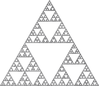
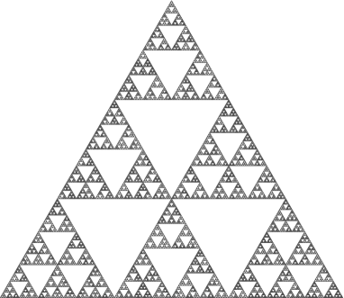
Figure 2: Examples of inhomogeneous Sierpinski gaskets $(T=\{2,3\})$.

If $L_{w}=\nu$ for all $w\in W_{*}$, then $G(L)$ is nothing but $\mathrm{SG}(\nu)$.

For $m\in{\mathbb{N}}$, let

$$V_{m}=\bigcup_{w\in\tilde{W}_{m}}\psi_{w}(V_{0}),$$

and let $V_{*}=\bigcup_{m\in{\mathbb{Z}}_{+}}V_{m}$. The closure of $V_{*}$ is equal to $G(L)$.

Next, we define reference measures on $G(L)$. Let

$${\mathcal{A}}^{(\nu)}=\Biggl{\{}q=\{q_{v}\}_{v\in S^{(\nu)}}\Biggm{|}q_{v}>0\text{ for all $v\in S^{(\nu)}$ and }\sum_{v\in S^{(\nu)}}q_{v}=1\Biggr{\}}$$

and

$${\mathcal{A}}=\Bigl{\{}q=\{q_{v}\}_{v\in S}\Bigm{|}\text{for each $\nu\in T$, }\{q_{v}\}_{v\in S^{(\nu)}}\in{\mathcal{A}}^{(\nu)}\Bigr{\}}.$$

For $q\in{\mathcal{A}}$, there exists a unique Borel probability measure $\lambda_{q}$ on $\Sigma$ such that

$$\lambda_{q}(\Sigma_{w})=\begin{cases}q_{w_{1}}\cdots q_{w_{m}}&\text{if }w=w_{1}\cdots w_{m}\in\tilde{W}_{m},\\ 0&\text{if }w\notin\tilde{W}_{*}.\end{cases}$$

We note that

$$\lambda_{q}(\Sigma\setminus\tilde{\Sigma})=\lim_{m\to\infty}\lambda_{q}\Biggl{(}\Sigma\setminus\bigcup_{w\in\tilde{W}_{m}}\Sigma_{w}\Biggr{)}=0.$$

In what follows, $q_{w}$ denotes $q_{w_{1}}\cdots q_{w_{m}}$ for $w=w_{1}\cdots w_{m}\in W_{m}$. By definition, $q_{\emptyset}=1$. The Borel probability measure $\mu_{q}$ on $G(L)$ is defined by $\mu_{q}=(\pi|_{\tilde{\Sigma}})_{*}\lambda_{q}$, that is, the image measure of $\lambda_{q}$ by $\pi|_{\tilde{\Sigma}}\colon\tilde{\Sigma}\to G(L)$. It is easy to see that $\mu_{q}$ has full support and does not charge any one points. When $T=\{\nu\}$, $\mu_{q}$ is a self-similar measure on $G(L)=\mathrm{SG}(\nu)$.

We next construct a Dirichlet form on $G(L)$. Let $r_{i^{\nu}}=r^{(\nu)}$ for $i^{\nu}\in S$, and $r_{w}=r_{w_{1}}\cdots r_{w_{m}}$ for $w=w_{1}\cdots w_{m}\in W_{m}$. By definition, $r_{\emptyset}=1$. For $m\in{\mathbb{Z}}_{+}$, let

$${\mathcal{E}}^{(m)}(x,y)=\sum_{w\in\tilde{W}_{m}}\frac{1}{r_{w}}Q(x\circ\psi_{w}|_{V_{0}},y\circ\psi_{w}|_{V_{0}}),\quad x,y\in l(V_{m}).$$

From (2.1) and (2.2), it holds that for every $m\in{\mathbb{Z}}_{+}$ and $x\in l(V_{m})$,

$${\mathcal{E}}^{(m)}(x,x)=\inf\{{\mathcal{E}}^{(m+1)}(y,y)\mid y\in l(V_{m+1})\text{ and }y|_{V_{m}}=x\}.$$

Thus, for any $x\in l(V_{*})$, the sequence $\{{\mathcal{E}}^{(m)}(x|_{V_{m}},x|_{V_{m}})\}_{m=0}^{\infty}$ is non-decreasing. We define

$${\mathcal{F}} =\left\{f\in C(G(L))\;\middle|\;\lim_{m\to\infty}{\mathcal{E}}^{(m)}(f|_{V_{m}},f|_{V_{m}})<\infty\right\},$$

$${\mathcal{E}}(f,g) =\lim_{m\to\infty}{\mathcal{E}}^{(m)}(f|_{V_{m}},g|_{V_{m}}),\quad f,g\in{\mathcal{F}},$$

where $C(G(L))$ denotes the set of all real-valued continuous functions on $G(L)$. Then, $({\mathcal{E}},{\mathcal{F}})$ is a resistance form and also a strongly local regular Dirichlet form on $L^{2}(G(L),\mu_{q})$ for any $q\in{\mathcal{A}}$ (see [7] and [12, Chapter 2]). Here, $C(G(L))$ is regarded as a subspace of $L^{2}(G(L),\mu_{q})$. We equip ${\mathcal{F}}$ with the inner product $(f,g)_{\mathcal{F}}:={\mathcal{E}}(f,g)+\int_{G(L)}fg\,d\mu_{q}$ as usual.

The energy measure $\mu_{\langle f\rangle}$ of $f\in{\mathcal{F}}$ is a finite Borel measure on $G(L)$, which is characterized by

$$\int_{G(L)}g\,d\mu_{\langle f\rangle}=2{\mathcal{E}}(f,fg)-{\mathcal{E}}(f^{2},g),\quad g\in{\mathcal{F}}.$$

By letting $g\equiv 1$, the total mass of $\mu_{\langle f\rangle}$ is $2{\mathcal{E}}(f,f)$. Another expression of $\mu_{\langle f\rangle}$ is discussed in Section 3.

We introduce the following conditions for $q=\{q_{v}\}_{v\in S}\in{\mathcal{A}}$ to describe our main theorem.

1. $q_{i^{\nu}}\neq r^{(\nu)}$ for all $i\in S_{0}$ and $\nu\in T$.

2. For each $l_{0},l_{1}\in{\mathbb{N}}$, there exists $l_{2}\in{\mathbb{N}}$ such that the following ($\star$) holds for $\mu_{q}$-a.e. $\omega\in\Sigma$:

   • there exist infinitely many $k\in{\mathbb{Z}}_{+}$ such that, for every $i,j\in S_{0}$,

     $$[\omega]_{k}i^{\nu_{k+1}}\cdots i^{\nu_{k+l_{0}}}j^{\nu_{k+l_{0}+1}}\cdots j^{\nu_{k+l_{0}+l_{1}}}j^{\nu_{k+l_{0}+l_{1}+1}}\cdots j^{\nu_{k+l_{0}+l_{1}+l_{2}}}$$

     $$\in\tilde{W}_{k+l_{0}+l_{1}+l_{2}}$$ (2.5)

     implies that

     $$\{\nu_{m}\in T\mid k+l_{0}+1\leq m\leq k+l_{0}+l_{1}\}$$

     $$\subset\{\nu_{m}\in T\mid k+l_{0}+l_{1}+1\leq m\leq k+l_{0}+l_{1}+l_{2}\}.$$ (2.6)

Remark 2.3

1. Condition ($\star$) is meaningful only for $\omega\in\tilde{\Sigma}$.

2. For $\omega\in\tilde{\Sigma}$, $k\in{\mathbb{Z}}_{+}$, and $i,j\in S_{0}$, the elements $\nu_{k+1},\nu_{k+2},\dots,\nu_{k+l_{0}+l_{1}+l_{2}}\in T$ so that (2.5) holds are uniquely determined. Indeed, $\nu_{k+1}=L_{[\omega]_{k}}$, $\nu_{k+2}=L_{[\omega]_{k}i^{\nu_{k+1}}}$, $\nu_{k+3}=L_{[\omega]_{k}i^{\nu_{k+1}}i^{\nu_{k+2}}}$, and so on.

3. A simple sufficient condition for (2.6) is

   $$\{\nu_{m}\mid k+l_{0}+l_{1}+1\leq m\leq k+l_{0}+l_{1}+l_{2}\}=T.$$ (2.7)

Theorem 2.4

Let $q\in{\mathcal{A}}$. Suppose that Condition (A) or (B) holds. Then, $\mu_{\langle f\rangle}$ and $\mu_{q}$ are mutually singular for every $f\in{\mathcal{F}}$.

We provide some typical examples.

Example 2.5

Let $\nu\in T$ and define $L=\{L_{w}\}_{w\in W_{*}}$ by $L_{w}=\nu$ for all $w\in W_{*}$. Then, $G(L)$ is equal to $\mathrm{SG}(\nu)$. In this case, Condition ($\star$) is trivially satisfied for all $\omega\in\tilde{\Sigma}$ by letting $l_{2}=1$ because both sides of (2.6) are equal to $\{\nu\}$. Thus, by Theorem 2.4, $\mu_{\langle f\rangle}\perp\mu_{q}$ for every $f\in{\mathcal{F}}$ and $q\in{\mathcal{A}}$. This singularity has been proved in [10] already.

Example 2.6

Take any sequence $\{\tau_{m}\}_{m\in{\mathbb{Z}}_{+}}\in T^{{\mathbb{Z}}_{+}}$ and let $L_{w}=\tau_{|w|}$ for $w\in W_{*}$. The set $G(L)$ associated with $L=\{L_{w}\}_{w\in W_{*}}$ has been studied in, e.g., [6, 3, 11], and called a scale irregular Sierpinski gasket.

1. Let $q=\{q_{w}\}_{w\in S}\in{\mathcal{A}}$ be given by $q_{v}=N(\nu)^{-1}$ for $v\in S^{(\nu)}$. The associated measure $\mu_{q}$ is regarded as a uniform measure on $G(L)$. Since $N(\nu)^{-1}<\nu^{-1}$, Condition (A) holds from Lemma 2.1. Therefore, $\mu_{\langle f\rangle}\perp\mu_{q}$ for any $f\in{\mathcal{F}}$ from Theorem 2.4. This case was discussed in [11, Section 5].

2. 1. Suppose that there exists $l_{2}\in{\mathbb{N}}$ such that $\{\tau_{k+1},\tau_{k+2},\dots,\tau_{k+l_{2}}\}=T$ for infinitely many $k\in{\mathbb{Z}}_{+}$. Then, Condition ($\star$) is satisfied for all $\omega\in\tilde{\Sigma}$, in view of (2.7).

   2. Suppose that for each $l\in{\mathbb{N}}$ there exists $k\in{\mathbb{Z}}_{+}$ such that $\tau_{k+1}=\tau_{k+2}=\dots=\tau_{k+l}$. Then, Condition ($\star$) with $l_{2}=1$ is satisfied for all $\omega\in\tilde{\Sigma}$ and $l_{0},l_{1}\in{\mathbb{N}}$, but (2.7) may fail to hold for any $l_{2}$.

   In either case, $\mu_{\langle f\rangle}\perp\mu_{q}$ for any $f\in{\mathcal{F}}$ and any $q\in{\mathcal{A}}$ from Theorem 2.4.

Example 2.7

Let $\rho$ be a probability measure on $T$ with full support. We take a family of $T$-valued i.i.d. random variables $\{L_{w}(\cdot)\}_{w\in W_{*}}$ with distribution $\rho$ that are defined on some probability space $(\hat{\Omega},\hat{\mathcal{B}},\hat{P})$. For each $\hat{\omega}\in\hat{\Omega}$, we can define an inhomogeneous Sierpinski gasket $G(L(\hat{\omega}))$ associated with $L(\hat{\omega}):=\{L_{w}(\hat{\omega})\}_{w\in W_{*}}$. This is called a random recursive Sierpinski gasket [7]. Then, the following holds.

Theorem 2.8

For $\hat{P}$-a.s. $\hat{\omega}$, $G(L(\hat{\omega}))$ satisfies Condition (B) for all $q\in{\mathcal{A}}$. That is, for $\hat{P}$-a.s. $\hat{\omega}$, the Dirichlet form on $G(L(\hat{\omega}))$ can apply Theorem 2.4 for all $q\in{\mathcal{A}}$ to conclude that the energy measures and $\mu_{q}$ are mutually singular for all $q\in{\mathcal{A}}$.

Theorems 2.4 and 2.8 are proved in Section 4.

3 Preliminary lemmas

In this section, we provide the necessary concepts and lemmas for proving Theorem 2.4. We fix $L=\{L_{w}\}_{w\in W_{*}}\in T^{W_{*}}$ and $q\in{\mathcal{A}}$ and retain the notation used in the previous section.

For $w\in\tilde{W}_{*}$, let $K_{w}$ denote $\pi(\Sigma_{w}\cap\tilde{\Sigma})\,({}=\psi_{w}(\tilde{K})\cap G(L))$.

Let $m\in{\mathbb{Z}}_{+}$ and $x\in l(V_{m})$. There exists a unique $h\in{\mathcal{F}}$ that attains

$$\inf\{{\mathcal{E}}(f,f)\mid f\in{\mathcal{F}}\text{ and }f|_{V_{m}}=x\}.$$

We call such $h$ a piecewise harmonic (more precisely, an $m$-harmonic) function. When $m=0$, $h$ is called a harmonic function and is denoted by $\iota(x)$.

Lemma 3.1

For $f\in{\mathcal{F}}$ and $m\in{\mathbb{Z}}_{+}$, let $f_{m}$ be an $m$-harmonic function such that $f_{m}=f$ on $V_{m}$. Then, $f_{m}$ converges to $f$ in ${\mathcal{F}}$ as $m\to\infty$. In particular, the totality of piecewise harmonic functions is dense in ${\mathcal{F}}$.

Proof 3.2

The proof is standard. From the maximum principle (see, e.g., [12, Lemma 2.2.3]),

$$\min_{K_{w}}f\leq\min_{\psi_{w}(V_{0})}f=\min_{K_{w}}f_{m}\leq\max_{K_{w}}f_{m}=\max_{\psi_{w}(V_{0})}f\leq\max_{K_{w}}f$$

for any $w\in\tilde{W}_{m}$. Therefore, $f_{m}$ converges to $f$ uniformly on $G(L)$, in particular, in $L^{2}(G(L),\mu_{q})$ as $m\to\infty$. Because $\{f_{m}\}_{m\in{\mathbb{Z}}_{+}}$ is bounded in ${\mathcal{F}}$, it converges to $f$ weakly in ${\mathcal{F}}$. Because $\lim_{m\to\infty}(f_{m},f_{m})_{\mathcal{F}}=(f,f)_{\mathcal{F}}$, $f_{m}$ actually converges to $f$ strongly in ${\mathcal{F}}$.

Let $v\in W_{*}$. We define $L^{[v]}=\{L_{w}^{[v]}\}_{w\in W_{*}}\in T^{W_{*}}$ by $L_{w}^{[v]}=L_{vw}$. Then, we can define a strongly local regular Dirichlet form $({\mathcal{E}}^{[v]},{\mathcal{F}}^{[v]})$ on $L^{2}(G(L^{[v]}),\mu_{q}^{[v]})$, where $\mu_{q}^{[v]}$ is defined in the same way as $\mu_{q}$ with $L$ replaced by $L^{[v]}$. The energy measure of $f\in{\mathcal{F}}^{[v]}$ is denoted by $\mu_{\langle f\rangle}^{[v]}$. The following lemma is proved in a straightforward manner by going back to the above definition.

Lemma 3.3

1. Let $f\in{\mathcal{F}}$ and $m\in{\mathbb{N}}$. For each $v\in\tilde{W}_{m}$, $f^{[v]}:=f\circ\psi_{v}|_{G(L^{[v]})}$ belongs to ${\mathcal{F}}^{[v]}$. Moreover, it holds that

   $${\mathcal{E}}(f,f)=\sum_{v\in\tilde{W}_{m}}\frac{1}{r_{v}}{\mathcal{E}}^{[v]}(f^{[v]},f^{[v]})$$ (3.1)

   and

   $$\mu_{\langle f\rangle}=\sum_{v\in\tilde{W}_{m}}\frac{1}{r_{v}}(\psi_{v}|_{G(L^{[v]})})_{*}\mu_{\langle f^{[v]}\rangle}^{[v]}.$$ (3.2)

   If $f$ is an $m$-harmonic function, then $f^{[v]}$ is a harmonic function with respect to $({\mathcal{E}}^{[v]},{\mathcal{F}}^{[v]})$.

2. It holds that

   $$\mu_{q}=\sum_{v\in\tilde{W}_{m}}{q_{v}}(\psi_{v}|_{G(L^{[v]})})_{*}\mu_{q}^{[v]}.$$ (3.3)

By applying (3.1) with ${\mathcal{E}}$ replaced by ${\mathcal{E}}^{[\xi]}$ for $\xi\in\tilde{W}_{*}$ to $f=\iota(x)$ for $x\in l(V_{0})$, we obtain the following identity as a special case:

$$r_{\xi}^{-1}Q(A_{\xi}x)=\sum_{\zeta\in W_{m};\ \xi\zeta\in\tilde{W}_{*}}r_{\xi\zeta}^{-1}Q(A_{\xi\zeta}x),\quad m\in{\mathbb{Z}}_{+}.$$ (3.4)

Let $f\in{\mathcal{F}}$. For each $m\in{\mathbb{Z}}_{+}$, let $\lambda_{\langle f\rangle}^{(m)}$ be a measure on $W_{m}$ defined as

$$\lambda_{\langle f\rangle}^{(m)}(C)=2\sum_{v\in C\cap\tilde{W}_{m}}r_{v}^{-1}{\mathcal{E}}^{[v]}(f^{[v]},f^{[v]}),\quad C\subset W_{m}.$$

Then, we can verify that $\{\lambda_{\langle f\rangle}^{(m)}\}_{m\in{\mathbb{Z}}_{+}}$ are consistent in the sense that $\lambda_{\langle f\rangle}^{(m)}(C)=\lambda_{\langle f\rangle}^{(m+1)}(C\times S)$. By the Kolmogorov extension theorem, there exists a unique Borel measure $\lambda_{\langle f\rangle}$ on $\Sigma$ such that

$$\lambda_{\langle f\rangle}(\Sigma_{C})=\lambda_{\langle f\rangle}^{(m)}(C)\quad\text{for any }m\in{\mathbb{Z}}_{+},\ C\subset W_{m},$$

where $\Sigma_{C}=\bigcup_{v\in C}\Sigma_{v}$. It is easy to see that $\lambda_{\langle f\rangle}(\Sigma\setminus\tilde{\Sigma})=0$.

In particular, if $f=\iota(x)$ for $x\in l(V_{0})$, we have

$$\lambda_{\langle\iota(x)\rangle}(\Sigma_{C})=2\sum_{v\in C\cap\tilde{W}_{m}}r_{v}^{-1}Q(A_{v}x),\quad C\subset W_{m}.$$ (3.5)

For simplicity, we write $\lambda_{\langle x\rangle}$ for $\lambda_{\langle\iota(x)\rangle}$.

Lemma 3.4

For $f\in{\mathcal{F}}$, $(\pi|_{\tilde{\Sigma}})_{*}\lambda_{\langle f\rangle}=\mu_{\langle f\rangle}$.

Proof 3.5

This lemma is proved in [9, Lemma 4.1] when $T$ is a one-point set. In the general case, it suffices to modify the proof line by line by using Lemma 3.3 as a substitution of the self-similar property. We provide a proof here for the reader’s convenience.

We define a set function $\chi_{m}$ for $m\in{\mathbb{Z}}_{+}$ by

$$\chi_{m}(A)=\sum_{v\in\tilde{W}_{m}}\frac{1}{r_{v}}\mu_{\langle f^{[v]}\rangle}^{[v]}(\pi(\sigma_{v}^{-1}(A)))$$

for a $\sigma$-compact subset $A$ of $\tilde{\Sigma}$.

Let $B$ be a closed subset of $G(L)$. For $v\in\tilde{W}_{m}$,

$$(\psi_{v}|_{G(L^{[v]})})^{-1}(B) =\pi\bigl{(}(\pi|_{\tilde{\Sigma}})^{-1}((\psi_{v}|_{G(L^{[v]})})^{-1}(B))\bigr{)}$$

$$=\pi\bigl{(}\sigma_{v}^{-1}((\pi|_{\tilde{\Sigma}})^{-1}(B))\bigr{)}.$$

Therefore, $\mu_{\langle f\rangle}(B)=\chi_{m}\bigl{(}(\pi|_{\tilde{\Sigma}})^{-1}(B)\bigr{)}$ from (3.2).

For $C\subset\tilde{W}_{m}$,

$$\lambda_{\langle f\rangle}(\Sigma_{C}) =\lambda_{\langle f\rangle}^{(m)}(C)$$

$$=2\sum_{v\in C}r_{v}^{-1}{\mathcal{E}}^{[v]}(f^{[v]},f^{[v]})$$

$$=\sum_{v\in\tilde{W}_{m}}r_{v}^{-1}\mu_{\langle f^{[v]}\rangle}^{[v]}\bigl{(}\pi(\sigma_{v}^{-1}(\Sigma_{C}))\bigr{)}$$

$$=\chi_{m}(\Sigma_{C}).$$

Here, in the third equality, we used the identity

$$\pi(\sigma_{v}^{-1}(\Sigma_{C}))=\begin{cases}G(L^{[v]})&\text{if }v\in C,\\ \emptyset&\text{otherwise}.\end{cases}$$

Let $F$ be a closed subset of $G(L)$. Then, $(\pi|_{\tilde{\Sigma}})^{-1}(F)$ is also closed in $\tilde{\Sigma}$. For $m\in{\mathbb{Z}}_{+}$, let $C_{m}=\bigl{\{}w\in\tilde{W}_{m}\bigm{|}\Sigma_{w}\cap(\pi|_{\tilde{\Sigma}})^{-1}(F)\neq\emptyset\bigr{\}}$. Then, $\{\Sigma_{C_{m}}\}_{m=0}^{\infty}$ is decreasing in $m$ and $\bigcap_{m\in{\mathbb{Z}}_{+}}\Sigma_{C_{m}}=(\pi|_{\tilde{\Sigma}})^{-1}(F)$. By using the monotonicity of $\chi_{m}$,

$$\mu_{\langle f\rangle}(F)=\chi_{m}\bigl{(}(\pi|_{\tilde{\Sigma}})^{-1}(F)\bigr{)}\leq\chi_{m}(\Sigma_{C_{m}})=\lambda_{\langle f\rangle}(\Sigma_{C_{m}}).$$

Letting $m\to\infty$, we have $\mu_{\langle f\rangle}(F)\leq\lambda_{\langle f\rangle}(F)$.

The inner regularity of $\mu_{\langle f\rangle}$ and $\lambda_{\langle f\rangle}$ implies that $\mu_{\langle f\rangle}(B)\leq\lambda_{\langle f\rangle}(B)$ for all Borel sets $B$. Because the total measures of $\mu_{\langle f\rangle}$ and $\lambda_{\langle f\rangle}$ are the same, we also have the reverse inequality by considering $G(L)\setminus B$ in place of $B$.

Let $i\in S_{0}$ and $\nu\in T$. From [12, Proposition A.1.1 and Theorem A.1.2], both $1$ and $r^{(\nu)}$ are simple eigenvalues of $A_{i}^{(\nu)}$, and the modulus of another eigenvalue $s^{(\nu)}$ of $A_{i}^{(\nu)}$ is less than $r^{(\nu)}$. In our situation, the eigenvectors are explicitly described: the eigenvectors of eigenvalues $1$, $r^{(\nu)}$, $s^{(\nu)}$ are constant multiples of

$$\mathbf{1}:=\begin{pmatrix}1\\ 1\\ 1\end{pmatrix},\quad\tilde{v}_{1}:=\begin{pmatrix}0\\ 1\\ 1\end{pmatrix},\quad y_{1}:=\begin{pmatrix}0\\ 1\\ -1\end{pmatrix}\quad\text{for }A_{1}^{(\nu)},$$

$$\mathbf{1},\phantom{{}:=\begin{pmatrix}1\\ 1\\ 1\end{pmatrix}{}}\quad\tilde{v}_{2}:=\begin{pmatrix}1\\ 0\\ 1\end{pmatrix},\quad y_{2}:=\begin{pmatrix}-1\\ 0\\ 1\end{pmatrix}\quad\text{for }A_{2}^{(\nu)},$$

$$\mathbf{1},\phantom{{}:=\begin{pmatrix}1\\ 1\\ 1\end{pmatrix}{}}\quad\tilde{v}_{3}:=\begin{pmatrix}1\\ 1\\ 0\end{pmatrix},\quad y_{3}:=\begin{pmatrix}1\\ -1\\ 0\end{pmatrix}\quad\text{for }A_{3}^{(\nu)},$$

respectively. Here, we identify $x\in l(V_{0})$ with $\begin{pmatrix}x(p_{1})\\ x(p_{2})\\ x(p_{3})\end{pmatrix}$. It is crucial for subsequent arguments that the eigenvectors of eigenvalue $r^{(\nu)}$ are independent of $\nu$.

Let $\tilde{l}(V_{0})$ be the set of all $x\in l(V_{0})$ such that $\sum_{p\in V_{0}}x(p)=0$. The orthogonal linear space of $\tilde{l}(V_{0})$ in $l(V_{0})$ is one-dimensional and spanned by $\mathbf{1}$. The function $\tilde{l}(V_{0})\ni x\mapsto Q(x,x)^{1/2}\in{\mathbb{R}}$ defines a norm on $\tilde{l}(V_{0})$. Let $P$ denote the orthogonal projection from $l(V_{0})$ onto $\tilde{l}(V_{0})$. For each $i\in S_{0}$, $u_{i}\in l(V_{0})$ denotes the column vector $(D_{p,p_{i}})_{p\in V_{0}}$.

Lemma 3.6 (see, e.g., [10, Lemma 5] and [12, Lemma A.1.4])

For each $i\in S_{0}$ and $\nu\in T$, $u_{i}$ is an eigenvector of ${\,}^{t}\!A_{i}^{(\nu)}$ with respect to the eigenvalue $r^{(\nu)}$. Moreover, $u_{i}\in\tilde{l}(V_{0})$.

We also note that $(u_{i},\mathbf{1})=(u_{i},y_{i})=0$. We take $v_{i}\in l(V_{0})$ such that $v_{i}$ is a constant multiple of $\tilde{v}_{i}$ and $(u_{i},v_{i})=1$.

Lemma 3.7

Let $i\in S_{0}$, $x\in l(V_{0})$, and $\boldsymbol{\nu}=\{\nu_{k}\}_{k\in{\mathbb{N}}}\in T^{\mathbb{N}}$. Then, it holds that

$$\lim_{n\to\infty}r_{i^{\nu_{1}}i^{\nu_{2}}\cdots i^{\nu_{n}}}^{-1}PA_{i^{\nu_{1}}i^{\nu_{2}}\cdots i^{\nu_{n}}}x=(u_{i},x)Pv_{i}$$ (3.6)

and

$$\lim_{n\to\infty}r_{i^{\nu_{1}}i^{\nu_{2}}\cdots i^{\nu_{n}}}^{-2}Q(A_{i^{\nu_{1}}i^{\nu_{2}}\cdots i^{\nu_{n}}}x)=(u_{i},x)^{2}Q(v_{i}).$$ (3.7)

Moreover, these convergences are uniform in $i\in S_{0}$, $x\in{\mathcal{C}}$, and $\boldsymbol{\nu}\in T^{\mathbb{N}}$, where ${\mathcal{C}}$ is the inverse image of an arbitrary compact set of $l(V_{0})$ by $P$.

Proof 3.8

Note that $PA_{i^{\nu_{1}}i^{\nu_{2}}\cdots i^{\nu_{n}}}\mathbf{1}=0$ and $r_{i^{\nu_{1}}i^{\nu_{2}}\cdots i^{\nu_{n}}}^{-1}A_{i^{\nu_{1}}i^{\nu_{2}}\cdots i^{\nu_{n}}}v_{i}=v_{i}$ for all $n$. Moreover, $|r_{i^{\nu_{1}}i^{\nu_{2}}\cdots i^{\nu_{n}}}^{-1}A_{i^{\nu_{1}}i^{\nu_{2}}\cdots i^{\nu_{n}}}y_{i}|\leq\theta^{n}|y_{i}|$, where $\theta=\max_{\nu\in T}|s^{(\nu)}/r^{(\nu)}|\in[0,1)$.

For $x\in l(V_{0})$ in general, we can decompose $x$ into $x=x_{1}\mathbf{1}+x_{2}v_{i}+x_{3}y_{i}$. By taking the inner product with $u_{i}$ on both sides, $(u_{i},x)=x_{2}(u_{i},v_{i})=x_{2}$. Therefore, (3.6) holds, and (3.7) follows immediately from (3.6). The uniformity of the convergences is evident from the argument above.

Although the next lemma can be confirmed by concrete calculation, we provide a proof that is applicable to more general situations.

Lemma 3.9

The following hold.

1. For every $i,j\in S_{0}$, $Q(v_{i},v_{i})=Q(v_{j},v_{j})>0$. For $j\in S_{0}$ and $i,i^{\prime}\in S_{0}\setminus\{j\}$, $(Dv_{j})(p_{i})=(Dv_{j})(p_{i^{\prime}})$.

2. For every $i,j\in S_{0}$, $(u_{i},v_{j})\neq 0$.

3. There exists $\delta_{0}>0$ such that, for each $i\in S_{0}$, there exists some $i^{\prime}\in S_{0}$ satisfying

   $$\bigl{|}|(Dv_{i})(p_{i})|-|(Dv_{i})(p_{i^{\prime}})|\bigr{|}\geq\delta_{0}.$$ (3.8)

Proof 3.10

1. This is proved in [10, Lemma 10] in more-general situations.

2. Note that $(u_{j},v_{j})=1$. From (1), $(u_{i},v_{j})=(Dv_{j})(p_{i})$ is independent of $i\in S_{0}\setminus\{j\}$. Moreover, $0=(Dv_{j},\mathbf{1})=\sum_{i\in S_{0}}(u_{i},v_{j})$. Therefore, $(u_{i},v_{j})=-1/(\#S_{0}-1)=-1/2$ for $i\in S_{0}\setminus\{j\}$.

3. From the proof of (2), we can take $\delta_{0}=1/2$.

The following are simple estimates used in the proofs of Lemma 4.1 and Theorem 2.4.

Lemma 3.11

Let $s,t>0$ and $a>0$. If $\left|\log(t/s)\right|\geq a$, then

$$|t-s|\geq(1-e^{-a})\max\{s,t\}.$$

Proof 3.12

We may assume that $s\leq t$. Then, $t/s\geq e^{a}$, which implies $t-s\geq t-te^{-a}=t(1-e^{-a})$.

Lemma 3.13

Let $d\in{\mathbb{N}}$ and

$${\mathcal{P}}_{d}=\left\{a=(a_{1},\dots,a_{d})\in{\mathbb{R}}^{d}\;\middle|\;a_{k}\geq 0\text{ for all $k=1,\dots,d$, and }\sum_{k=1}^{d}a_{k}=1\right\}.$$

For $a=(a_{1},\dots,a_{d}),\ b=(b_{1},\dots,b_{d})\in{\mathcal{P}}_{d}$, it holds that

$$\sum_{k=1}^{d}\sqrt{a_{k}b_{k}}\leq 1-\frac{|a-b|_{{\mathbb{R}}^{d}}^{2}}{8}.$$

Proof 3.14

Since all $a_{k}$ and $b_{k}$ are dominated by $1$,

$$\sqrt{a_{k}b_{k}} =\frac{a_{k}+b_{k}}{2}-\frac{(a_{k}-b_{k})^{2}}{2(\sqrt{a_{k}}+\sqrt{b_{k}})^{2}}$$

$$\leq\frac{a_{k}+b_{k}}{2}-\frac{(a_{k}-b_{k})^{2}}{8}.$$

Taking the sum with respect to $k$ on both sides, we arrive at the conclusion.

At the end of this section, we introduce a general sufficient condition for singularity of two measures. For $z\in{\mathbb{R}}$, let

$$z^{\oplus}=\begin{cases}1/z&(z\neq 0)\\ 0&(z=0).\end{cases}$$

Theorem 3.15

Let $(\Omega,{\mathcal{B}},\{{\mathcal{B}}_{n}\}_{n\in{\mathbb{Z}}_{+}})$ be a measurable space equipped with a filtration such that ${\mathcal{B}}=\bigvee_{n\in{\mathbb{Z}}_{+}}{\mathcal{B}}_{n}$. Let $P_{1}$ and $P_{2}$ be two probability measures on $(\Omega,{\mathcal{B}})$. Suppose that, for each $n\in{\mathbb{Z}}_{+}$, $P_{2}|_{{\mathcal{B}}_{n}}$ is absolutely continuous with respect to $P_{1}|_{{\mathcal{B}}_{n}}$. Let $z_{n}$ be the Radon–Nikodym derivative $d(P_{2}|_{{\mathcal{B}}_{n}})/d(P_{1}|_{{\mathcal{B}}_{n}})$ for $n\in{\mathbb{Z}}_{+}$ and $\alpha_{n}=z_{n}z_{n-2}^{\oplus}$ for $n\geq 2$. If

$$\sum_{n=2}^{\infty}\left(1-{\mathbb{E}}^{P_{1}}[\sqrt{\alpha_{n}}\mid{\mathcal{B}}_{n-2}]\right)=\infty\quad P_{1}\text{-a.s.}$$ (3.9)

holds, then $P_{1}$ and $P_{2}$ are mutually singular. Here, ${\mathbb{E}}^{P_{1}}[{}\mathrel{\cdot}|{\mathcal{B}}_{n-2}]$ denotes the conditional expectation for $P_{1}$ given ${\mathcal{B}}_{n-2}$.

Proof 3.16

We modify the proof of [9, Theorem 4.1]. By [14, Theorem VII.6.1], $z_{\infty}:=\lim_{n\to\infty}z_{n}$ exists $(P_{1}+P_{2})$-a.e. and

$$P_{2}(A)=\int_{A}z_{\infty}\,dP_{1}+P_{2}(A\cap\{z_{\infty}=\infty\}),\quad A\in{\mathcal{B}}.$$ (3.10)

Moreover, $P_{1}$ and $P_{2}({}\cdot{}\mathrel{\cap}\{z_{\infty}=\infty\})$ are mutually singular.

Let

$$Z_{1} =\left\{\sum_{k=1}^{\infty}\bigl{(}1-{\mathbb{E}}^{P_{1}}[\sqrt{\alpha_{2k}}\mid{\mathcal{B}}_{2(k-1)}]\bigr{)}=\infty\right\},$$

$$Z_{2} =\left\{\sum_{k=1}^{\infty}\bigl{(}1-{\mathbb{E}}^{P_{1}}[\sqrt{\alpha_{2k+1}}\mid{\mathcal{B}}_{2(k-1)+1}]\bigr{)}=\infty\right\}.$$

From (3.9), $P_{1}(Z_{1}\cup Z_{2})=1$. Considering the two filtrations $\{{\mathcal{B}}_{2k}\}_{k\in{\mathbb{Z}}_{+}}$ and $\{{\mathcal{B}}_{2k+1}\}_{k\in{\mathbb{Z}}_{+}}$ and following the proof of [14, Theorem VII.6.4], we have $\{z_{\infty}=\infty\}=Z_{1}=Z_{2}$ up to $P_{2}$-null sets. Therefore, $z_{\infty}=\infty$ $P_{2}$-a.e. on $Z_{1}\cup Z_{2}$. Applying (3.10) to $A=\Omega\setminus(Z_{1}\cup Z_{2})$, which is a $P_{1}$-null set, we have $P_{2}(A)=P_{2}(A\cap\{z_{\infty}=\infty\})$, that is, $z_{\infty}=\infty$ $P_{2}$-a.e. on $A$. Thus, $P_{2}(z_{\infty}=\infty)=1$ and we conclude that $P_{1}$ and $P_{2}$ are mutually singular.

4 Proof of the main results

We introduce some notation. Let ${\mathcal{K}}$ be a closed set of $l(V_{0})$ that is defined as

$${\mathcal{K}}=\{x\in l(V_{0})\mid 2Q(x,x)=1\}.$$

For $l_{0}\in{\mathbb{Z}}_{+}$ and $l_{1},l_{2}\in{\mathbb{N}}$, let

$$L(l_{0},l_{1},l_{2})=\left\{\boldsymbol{\nu}=\{\nu_{k}\}_{k=1}^{\infty}\in T^{\mathbb{N}}\;\middle|\;\begin{array}[]{l}\{\nu_{k}\mid l_{0}+1\leq k\leq l_{0}+l_{1}\}\\ \subset\{\nu_{k}\mid l_{0}+l_{1}+1\leq k\leq l_{0}+l_{1}+l_{2}\}\end{array}\right\}.$$

We define several constants as follows:

$$\beta_{1} :=\min\{|(u_{i},v_{j})|\mid i,j\in S_{0}\}=\min\{|(Dv_{i})(p)|\mid i\in S_{0},\ p\in V_{0}\},$$

$$\beta_{2} :=\min\left\{\left|\log(r_{v}/q_{v})\right|\mid v\in S,\ r_{v}\neq q_{v}\right\}>0,$$

$$\beta_{3} :=\min\{q_{v}\mid v\in S\}>0,$$

$$\beta_{4} :=\min\{r^{(\nu)}\mid\nu\in T\}>0,$$

$$\beta_{5} :=2Q(v_{i},v_{i})>0\quad(i\in S_{0}).$$

By Lemma 3.9(2), $\beta_{1}>0$. In the definition of $\beta_{2}$, $\min\emptyset=1$ by convention. By Lemma 3.9(1), $\beta_{5}$ is independent of the choice of $i$.

We fix $q\in{\mathcal{A}}$. The following is a key lemma for proving Theorem 2.4.

Lemma 4.1

1. There exist $N\in{\mathbb{N}}$ and $N^{\prime}\in{\mathbb{N}}$ such that, for any $l\in{\mathbb{N}}$, there exists $\gamma>0$ satisfying the following. For all $\boldsymbol{\nu}=\{\nu_{k}\}_{k=1}^{\infty}\in L(N,N^{\prime},l)$ and $x\in{\mathcal{K}}$, there exist

   $$i =i(x)\in S_{0},$$

   $$j =j(x,\nu_{1},\nu_{2},\dots,\nu_{N})\in S_{0},$$

   $$m =m(l,x,\nu_{1},\nu_{2},\dots,\nu_{N+N^{\prime}+l})\in\{N^{\prime},N^{\prime}+1,\dots,N^{\prime}+l\}$$

   such that

   $$|2r_{\xi}^{-1}Q(A_{\xi}x)-q_{\xi}|\geq\gamma$$

   with $\xi=i^{\nu_{1}}\cdots i^{\nu_{N}}j^{\nu_{N+1}}\cdots j^{\nu_{N+m}}$. Here, “$j=j(x,\nu_{1},\nu_{2},\dots,\nu_{N})$” means that “$j$ depends only on $x,\nu_{1},\nu_{2},\dots,\nu_{N}$,” and so on.

2. If Condition (A) holds, then the claim of item (1) holds with “$\boldsymbol{\nu}=\{\nu_{k}\}_{k=1}^{\infty}\in L(N,N^{\prime},l)$” replaced by “$\boldsymbol{\nu}=\{\nu_{k}\}_{k=1}^{\infty}\in T^{\mathbb{N}}$.”

Proof 4.2

(1) Let $\varphi$ be a continuous function on $l(V_{0})$ that is defined as

$$\varphi(x)=\sum_{i\in S_{0}}(u_{i},x)^{2}.$$

Since the range of $\varphi$ on ${\mathcal{K}}$ is equal to that on a compact set $P({\mathcal{K}})$, $\varphi$ attains a minimum on ${\mathcal{K}}$, say $\beta_{6}$. Let $x\in{\mathcal{K}}$. Because

$$0<Q(x,x)=(-Dx,x)=-\sum_{i\in S_{0}}(u_{i},x)x(p_{i}),$$

$(u_{i},x)\neq 0$ for some $i\in S_{0}$. This implies that $\varphi(x)>0$. (In fact, we can confirm that $\varphi(x)\equiv 3/2$.) Thus, $\beta_{6}>0$. Define $\delta^{\prime}=\beta_{6}/\#S_{0}=\beta_{6}/3$ and ${\mathcal{K}}_{i}=\{x\in{\mathcal{K}}\mid(u_{i},x)^{2}\geq\delta^{\prime}\}$ for $i\in S_{0}$. It holds that ${\mathcal{K}}=\bigcup_{i\in S_{0}}{\mathcal{K}}_{i}$.

We fix $x\in{\mathcal{K}}$. There exists $i\in S_{0}$ such that $x\in{\mathcal{K}}_{i}$. From Lemma 3.9(3), there exists $i^{\prime}\in S_{0}$ such that (3.8) holds. By keeping in mind that $(Dv_{i})(p_{i})=1$, it follows that

$$\bigl{|}(Dv_{i})(p_{i})^{2}-(Dv_{i})(p_{i^{\prime}})^{2}\bigr{|} =\bigl{|}1+|(Dv_{i})(p_{i^{\prime}})|\bigr{|}\,\bigl{|}|(Dv_{i})(p_{i})|-|(Dv_{i})(p_{i^{\prime}})|\bigr{|}$$

$$\geq\delta_{0}.$$ (4.1)

Let $\boldsymbol{\nu}=\{\nu_{k}\}_{k\in{\mathbb{N}}}\in T^{\mathbb{N}}$ and define $x_{n}=r_{i^{\nu_{1}}\cdots i^{\nu_{n}}}^{-1}A_{i^{\nu_{1}}\cdots i^{\nu_{n}}}x$ for $n\in{\mathbb{N}}$. From Lemma 3.6,

$$(u_{i},x_{n})=(r_{i^{\nu_{1}}\cdots i^{\nu_{n}}}^{-1}{}^{t}\!A_{i^{\nu_{1}}\cdots i^{\nu_{n}}}u_{i},x)=(u_{i},x).$$ (4.2)

Let $\delta_{1}=\sqrt{\delta^{\prime}}\beta_{1}/2$ and $\delta_{2}=\delta^{\prime}\delta_{0}/3$. By Lemma 3.7, there exists $N\in{\mathbb{N}}$ independent of the choice of $x$, $i$, and $\boldsymbol{\nu}$ such that, for all $p\in V_{0}$,

$$\bigl{|}|(Dx_{N})(p)|-|(u_{i},x)(Dv_{i})(p)|\bigr{|} \leq\delta_{1}$$ (4.3)

and

$$\bigl{|}(Dx_{N})(p)^{2}-(u_{i},x)^{2}(Dv_{i})(p)^{2}\bigr{|} \leq\delta_{2}.$$ (4.4)

From (4.2) and (4.3), for any $j\in S_{0}$,

$$|(u_{j},x_{N})| =|(Dx_{N})(p_{j})|$$

$$\geq|(u_{i},x)(Dv_{i})(p_{j})|-\delta_{1}$$

$$\geq\sqrt{\delta^{\prime}}\beta_{1}-\delta_{1}=\delta_{1}.$$

By Lemma 3.7,

$$\lim_{m\to\infty}r_{j^{\nu_{N+1}}\cdots j^{\nu_{N+m}}}^{-2}Q(A_{j^{\nu_{N+1}}\cdots j^{\nu_{N+m}}}x_{N}) =(u_{j},x_{N})^{2}Q(v_{j})$$

$$\geq\delta_{1}^{2}\beta_{5}/2>0.$$

This convergence is uniform in $x$, $i$, $j$, and $\boldsymbol{\nu}$ because $Px_{N}$ belongs to some compact set of ${\mathcal{K}}$ that is independent of them. We take $\delta_{3}=\beta_{5}\delta_{2}/2$. Then, there exists $N^{\prime}\in{\mathbb{N}}$ independent of $x$, $i$, $j$, and $\boldsymbol{\nu}$ such that, for every $n\geq N^{\prime}$,

$$\bigl{|}r_{j^{\nu_{N+1}}\cdots j^{\nu_{N+n}}}^{-2}Q(A_{j^{\nu_{N+1}}\cdots j^{\nu_{N+n}}}x_{N})-(u_{j},x_{N})^{2}Q(v_{j})\bigr{|}\leq\delta_{3}/4$$ (4.5)

and

$$\left|\log\frac{r_{j^{\nu_{N+1}}\cdots j^{\nu_{N+n-1}}}^{-2}Q(A_{j^{\nu_{N+1}}\cdots j^{\nu_{N+n-1}}}x_{N})}{r_{j^{\nu_{N+1}}\cdots j^{\nu_{N+n}}}^{-2}Q(A_{j^{\nu_{N+1}}\cdots j^{\nu_{N+n}}}x_{N})}\right|\leq\frac{\beta_{2}}{2}.$$ (4.6)

From (4.1) and (4.4),

$$\delta^{\prime}\delta_{0} \leq(u_{i},x)^{2}\bigl{|}(Dv_{i})(p_{i})^{2}-(Dv_{i})(p_{i^{\prime}})^{2}\bigr{|}$$

$$\leq\bigl{|}(u_{i},x)^{2}(Dv_{i})(p_{i})^{2}-(Dx_{N})(p_{i})^{2}\bigr{|}+\bigl{|}(Dx_{N})(p_{i})^{2}-(Dx_{N})(p_{i^{\prime}})^{2}\bigr{|}$$

$$\quad+\bigl{|}(Dx_{N})(p_{i^{\prime}})^{2}-(u_{i},x)^{2}(Dv_{i})(p_{i^{\prime}})^{2}\bigr{|}$$

$$\leq 2\delta_{2}+\bigl{|}(Dx_{N})(p_{i})^{2}-(Dx_{N})(p_{i^{\prime}})^{2}\bigr{|},$$

which implies that

$$\bigl{|}(Dx_{N})(p_{i})^{2}-(Dx_{N})(p_{i^{\prime}})^{2}\bigr{|}\geq\delta^{\prime}\delta_{0}-2\delta_{2}=\delta_{2}.$$

From the identity $(Dx_{N})(p_{j})=(u_{j},x_{N})$ $(j\in S_{0})$, we have

$$2\delta_{3} =\beta_{5}\delta_{2}$$

$$\leq\beta_{5}\bigl{|}(u_{i},x_{N})^{2}-(u_{i^{\prime}},x_{N})^{2}\bigr{|}$$

$$\leq\bigl{|}2Q(v_{i})(u_{i},x_{N})^{2}-q_{w}/r_{w}\bigr{|}+\bigl{|}2Q(v_{i^{\prime}})(u_{i^{\prime}},x_{N})^{2}-q_{w}/r_{w}\bigr{|},$$

where we choose $w=i^{\nu_{1}}\cdots i^{\nu_{N}}\in W_{N}$. Then, for either $j=i$ or $i^{\prime}$,

$$\bigl{|}2Q(v_{j})(u_{j},x_{N})^{2}-q_{w}/r_{w}\bigr{|}\geq\delta_{3}.$$ (4.7)

We fix such $j$. Take any $l\in{\mathbb{N}}$ and suppose $\boldsymbol{\nu}\in L(N,N^{\prime},l)$. There are two possibilities:

1. There exists some $k\in\{N^{\prime}+1,\dots,N^{\prime}+l\}$ such that $r_{j^{\nu_{N+k}}}\neq q_{j^{\nu_{N+k}}}$.

2. $r_{j^{\nu_{N+k}}}=q_{j^{\nu_{N+k}}}$ for all $k\in\{N^{\prime}+1,\dots,N^{\prime}+l\}$.

Suppose Case I). Let $w^{\prime}=j^{\nu_{N+1}}\cdots j^{\nu_{N+k-1}}\in W_{k-1}$. From (4.6) with $n=k$,

$$\frac{\beta_{2}}{2} \geq\left|\log\left(r_{j^{\nu_{N+k}}}^{2}\times\frac{Q(A_{j^{\nu_{N+1}}\cdots j^{\nu_{N+k-1}}}x_{N})}{Q(A_{j^{\nu_{N+1}}\cdots j^{\nu_{N+k}}}x_{N})}\right)\right|$$

$$=\left|\log\left(\frac{r_{j^{\nu_{N+k}}}}{q_{j^{\nu_{N+k}}}}\frac{2r_{ww^{\prime}}^{-1}Q(A_{ww^{\prime}}x)}{q_{ww^{\prime}}}\frac{q_{ww^{\prime}j^{\nu_{N+k}}}}{2r_{ww^{\prime}j^{\nu_{N+k}}}^{-1}Q(A_{ww^{\prime}j^{\nu_{N+k}}}x)}\right)\right|$$

$$\geq\beta_{2}-\left|\log\frac{2r_{ww^{\prime}}^{-1}Q(A_{ww^{\prime}}x)}{q_{ww^{\prime}}}\right|-\left|\log\frac{q_{ww^{\prime}j^{\nu_{N+k}}}}{2r_{ww^{\prime}j^{\nu_{N+k}}}^{-1}Q(A_{ww^{\prime}j^{\nu_{N+k}}}x)}\right|.$$

Therefore, either

$$\left|\log\frac{2r_{ww^{\prime}}^{-1}Q(A_{ww^{\prime}}x)}{q_{ww^{\prime}}}\right|\geq\frac{\beta_{2}}{4}\quad\text{or}\quad\left|\log\frac{q_{ww^{\prime}j^{\nu_{N+k}}}}{2r_{ww^{\prime}j^{\nu_{N+k}}}^{-1}Q(A_{ww^{\prime}j^{\nu_{N+k}}}x)}\right|\geq\frac{\beta_{2}}{4}$$

holds. Since $q_{ww^{\prime}}\geq q_{ww^{\prime}j^{\nu_{N+k}}}\geq\beta_{3}^{N+N^{\prime}+l}$, Lemma 3.11 implies that either

$$|2r_{ww^{\prime}}^{-1}Q(A_{ww^{\prime}}x)-q_{ww^{\prime}}|\geq(1-e^{-\beta_{2}/4})\beta_{3}^{N+N^{\prime}+l}$$ (4.8)

or

$$|2r_{ww^{\prime}j^{\nu_{N+k}}}^{-1}Q(A_{ww^{\prime}j^{\nu_{N+k}}}x)-q_{ww^{\prime}j^{\nu_{N+k}}}|\geq(1-e^{-\beta_{2}/4})\beta_{3}^{N+N^{\prime}+l}$$ (4.9)

holds.

Next, suppose Case II). Since $\boldsymbol{\nu}\in L(N,N^{\prime},l)$, $r_{j^{\nu_{N+k}}}=q_{j^{\nu_{N+k}}}$ for all $k\in\{1,\dots,N^{\prime}\}$. Let $\hat{w}=j^{\nu_{N+1}}\cdots j^{\nu_{N+N^{\prime}}}\in W_{N^{\prime}}$. Note that $q_{\hat{w}}=r_{\hat{w}}$. From (4.7) and (4.5),

$$\delta_{3} \leq|2Q(v_{j})(u_{j},x_{N})^{2}-q_{w}/r_{w}|$$

$$\leq|2Q(v_{j})(u_{j},x_{N})^{2}-2r_{\hat{w}}^{-2}Q(A_{\hat{w}}x_{N})|+|2r_{\hat{w}}^{-2}Q(A_{\hat{w}}x_{N})-q_{w\hat{w}}/r_{w\hat{w}}|$$

$$\leq\delta_{3}/2+\beta_{4}^{-(N+N^{\prime})}|2r_{w\hat{w}}^{-1}Q(A_{w\hat{w}}x)-q_{w\hat{w}}|.$$

Therefore,

$$|2r_{w\hat{w}}^{-1}Q(A_{w\hat{w}}x)-q_{w\hat{w}}|\geq\delta_{3}\beta_{4}^{N+N^{\prime}}/2.$$

In conclusion, it suffices to take

$$m=\begin{cases}k-1&\text{if \eqref{eq:I1} holds in Case I),}\\ k&\text{if \eqref{eq:I1} fails to hold in Case I),}\\ N^{\prime}&\text{in Case II)}\end{cases}$$

and

$$\gamma=\min\bigl{\{}(1-e^{-\beta_{2}/4})\beta_{3}^{N+N^{\prime}+l},\,\delta_{3}\beta_{4}^{N+N^{\prime}}/2\bigr{\}}.$$

(2) In the proof of (1), the condition that $\boldsymbol{\nu}\in L(N,N^{\prime},l)$ is used only in the discussion of Case II). Under Condition (A), Case II) never happens. Therefore, the arguments are valid for all $\boldsymbol{\nu}\in T^{\mathbb{N}}$.

Proof 4.3 (of Theorem 2.4)

Let $N$ and $N^{\prime}$ be natural numbers that are provided in Lemma 4.1. Under Condition (B), take $l_{2}\in{\mathbb{N}}$ associated with $l_{0}=N$ and $l_{1}=N^{\prime}$ in (B). Under Condition (A), take $l_{2}=1$.

Let $M=N+N^{\prime}+l_{2}$. For $n\in{\mathbb{Z}}_{+}$, let ${\mathcal{B}}_{n}$ denote the $\sigma$-field on $\Sigma$ that is generated by $\{\Sigma_{w}\mid w\in W_{Mn}\}$. Then, $\bigvee_{n=0}^{\infty}{\mathcal{B}}_{n}$ is equal to the Borel $\sigma$-field on $\Sigma$.

Take $x\in{\mathcal{K}}$. We first prove that $\lambda_{\langle x\rangle}$ and $\lambda_{q}$ are mutually singular. For each $n\in{\mathbb{Z}}_{+}$, $\lambda_{\langle x\rangle}|_{{\mathcal{B}}_{n}}$ is absolutely continuous with respect to $\lambda_{q}|_{{\mathcal{B}}_{n}}$. Indeed, if $\lambda_{q}(\Sigma_{w})=0$ for $w\in W_{Mn}$, then $w\notin\tilde{W}_{Mn}$, which implies $\lambda_{\langle x\rangle}(\Sigma_{w})=0$. Let $z_{n}$ denote the Radon–Nikodym derivative $d(\lambda_{\langle x\rangle}|_{{\mathcal{B}}_{n}})/d(\lambda_{q}|_{{\mathcal{B}}_{n}})$.

Under Condition (B), take $\omega=\omega_{1}\omega_{2}\cdots\in\tilde{\Sigma}$ such that Condition ($\star$) is satisfied, and let $k\in{\mathbb{Z}}_{+}$ in ($\star$). Under Condition (A), take $\omega\in\tilde{\Sigma}$ and $k\in{\mathbb{Z}}_{+}$ arbitrarily.

There exists a unique natural number $n\geq 2$ such that $M(n-2)\leq k<M(n-1)$. Let $w:=[\omega]_{M(n-2)}\in\tilde{W}_{M(n-2)}$ and $\xi\in W_{2M}$. Using (3.5), we have

$$z_{n-2}=\frac{\lambda_{\langle x\rangle}(\Sigma_{w})}{\lambda_{q}(\Sigma_{w})}=\frac{2r_{w}^{-1}Q(A_{w}x)}{q_{w}}\quad\text{on $\Sigma_{w}$}$$

and

$$z_{n}=\begin{cases}\dfrac{2r_{w\xi}^{-1}Q(A_{w\xi}x)}{q_{w\xi}}&\text{if }w\xi\in\tilde{W}_{Mn}\\ 0&\text{if }w\xi\notin\tilde{W}_{Mn}\end{cases}\quad\text{on $\Sigma_{w\xi}$}.$$

Then, on $\Sigma_{w\xi}$,

$$\alpha_{n}:=z_{n}z_{n-2}^{\oplus}=\begin{cases}\dfrac{Q(A_{w\xi}x)Q(A_{w}x)^{\oplus}}{q_{\xi}r_{\xi}}&\text{if }w\xi\in\tilde{W}_{Mn},\\ 0&\text{if }w\xi\notin\tilde{W}_{Mn}.\end{cases}$$

If $Q(A_{w}x)=0$, then $\alpha_{n}=0$ on $\Sigma_{w}$, which implies that

$$1-{\mathbb{E}}^{\lambda_{q}}[\sqrt{\alpha_{n}}\mid{\mathcal{B}}_{n-2}](\omega)=1.$$ (4.10)

Suppose that $Q(A_{w}x)\neq 0$. Let $x^{\prime}=A_{w}x\big{/}\sqrt{2Q(A_{w}x)}\in{\mathcal{K}}$. Then,

$${\mathbb{E}}^{\lambda_{q}}[\sqrt{\alpha_{n}}\mid{\mathcal{B}}_{n-2}](\omega) =\sum_{\xi\in W_{2M};\ w\xi\in\tilde{W}_{Mn}}\frac{q_{w\xi}}{q_{w}}\sqrt{\frac{Q(A_{w\xi}x)}{q_{\xi}r_{\xi}Q(A_{w}x)}}$$

$$=\sum_{\xi\in W_{2M};\ w\xi\in\tilde{W}_{Mn}}\sqrt{q_{\xi}\times 2r_{\xi}^{-1}Q(A_{\xi}x^{\prime})}$$

$$\leq 1-\frac{1}{8}\sum_{\xi\in W_{2M};\ w\xi\in\tilde{W}_{Mn}}\bigl{(}q_{\xi}-2r_{\xi}^{-1}Q(A_{\xi}x^{\prime})\bigr{)}^{2}.$$ (4.11)

Here, the last inequality follows from Lemma 3.13.

Take $\gamma>0$ in Lemma 4.1 associated with $l=l_{2}$. Let

$$w^{\prime}=\omega_{M(n-2)+1}\omega_{M(n-2)+2}\cdots\omega_{k}\in W_{k-M(n-2)}\quad\text{($w^{\prime}=\emptyset$ if $k=M(n-2)$)}$$

and $\gamma^{\prime}=\min\{\gamma,\beta_{3}^{M}\}$. Note that $q_{w^{\prime}}\geq\beta_{3}^{M}\geq\gamma^{\prime}$. We consider the following two cases:

1. $|q_{w^{\prime}}-2r_{w^{\prime}}^{-1}Q(A_{w^{\prime}}x^{\prime})|\geq\gamma\gamma^{\prime}/3$;

2. $|q_{w^{\prime}}-2r_{w^{\prime}}^{-1}Q(A_{w^{\prime}}x^{\prime})|<\gamma\gamma^{\prime}/3$.

Suppose Case i). Letting $I=\{\zeta\in W_{Mn-k}\mid ww^{\prime}\zeta\in\tilde{W}_{Mn}\}$, we have

$$\smashoperator[l]{\sum_{\xi\in W_{2M};\ w\xi\in\tilde{W}_{Mn}}^{}}\bigl{(}q_{\xi}-2r_{\xi}^{-1}Q(A_{\xi}x^{\prime})\bigr{)}^{2}$$

$$\geq\sum_{\zeta\in I}\bigl{(}q_{w^{\prime}\zeta}-2r_{w^{\prime}\zeta}^{-1}Q(A_{w^{\prime}\zeta}x^{\prime})\bigr{)}^{2}$$

$$\geq\Biggl{\{}\sum_{\zeta\in I}\bigl{(}q_{w^{\prime}\zeta}-2r_{w^{\prime}\zeta}^{-1}Q(A_{w^{\prime}\zeta}x^{\prime})\bigr{)}\Biggr{\}}^{2}\Biggl{(}\sum_{\zeta\in I}1\Biggr{)}^{-1}$$

$$=\left(q_{w^{\prime}}-2r_{w^{\prime}}^{-1}Q(A_{w^{\prime}}x^{\prime})\right)^{2}\left(\#I\right)^{-1}\qquad\text{(from \eqref{eq:Q})}$$

$$\geq(\gamma\gamma^{\prime}/3)^{2}(\#S)^{-2M}.$$

Next, suppose Case ii). We have

$$2r_{w^{\prime}}^{-1}Q(A_{w^{\prime}}x^{\prime}) >q_{w^{\prime}}-\gamma\gamma^{\prime}/3$$

$$\geq\gamma^{\prime}-\gamma^{\prime}/3=2\gamma^{\prime}/3.$$ (4.12)

In particular, $Q(A_{w^{\prime}}x^{\prime})\neq 0$. Let $x^{\prime\prime}=A_{w^{\prime}}x^{\prime}\big{/}\sqrt{2Q(A_{w^{\prime}}x^{\prime})}\in{\mathcal{K}}$. We make several choices in order as follows:

• Take $i\in S_{0}$ associated with $x^{\prime\prime}\in{\mathcal{K}}$ in Lemma 4.1.

• Take $\nu_{k+1},\nu_{k+2},\dots,\nu_{k+N}\in T$ such that $ww^{\prime}i^{\nu_{k+1}}i^{\nu_{k+2}}\cdots i^{\nu_{k+N}}\in\tilde{W}_{k+N}$; these are uniquely determined.

• Take $j\in S_{0}$ associated with $x^{\prime\prime}\in{\mathcal{K}}$, $i\in S_{0}$, and $\{\nu_{k+s}\}_{s=1}^{N}$ in Lemma 4.1.

• Take a unique sequence $\{\nu_{s}\}_{s=k+N+1}^{\infty}\subset T$ such that

  $$ww^{\prime}i^{\nu_{k+1}}i^{\nu_{k+2}}\cdots i^{\nu_{k+N}}j^{\nu_{k+N+1}}j^{\nu_{k+N+2}}\cdots j^{\nu_{k+N+t}}\in W_{k+N+t}$$

  for every $t\in{\mathbb{N}}$.

• Take $m\in\{N^{\prime},N^{\prime}+1,\dots,N^{\prime}+l_{2}\}$ associated with $x^{\prime\prime}\in{\mathcal{K}}$, $i\in S_{0}$, $j\in S_{0}$, and $\{\nu_{k+s}\}_{s=1}^{\infty}$ in Lemma 4.1.

Note that $\{\nu_{k+s}\}_{s=1}^{\infty}\in L(N,N^{\prime},l_{2})$ under Condition (B).

Let

$$\eta=i^{\nu_{k+1}}i^{\nu_{k+2}}\cdots i^{\nu_{k+N}}j^{\nu_{k+N+1}}j^{\nu_{k+N+2}}\cdots j^{\nu_{k+N+m}}\in W_{N+m}.$$

Then, letting $J=\{\eta^{\prime}\in W_{Mn-k-N-m}\mid ww^{\prime}\eta\eta^{\prime}\in\tilde{W}_{Mn}\}$, we have

$$\smashoperator[l]{\sum_{\xi\in W_{2M};\ w\xi\in\tilde{W}_{Mn}}^{}}\bigl{(}q_{\xi}-2r_{\xi}^{-1}Q(A_{\xi}x^{\prime})\bigr{)}^{2}$$

$$\geq\sum_{\eta^{\prime}\in J}\bigl{(}q_{w^{\prime}\eta\eta^{\prime}}-2r_{w^{\prime}\eta\eta^{\prime}}^{-1}Q(A_{w^{\prime}\eta\eta^{\prime}}x^{\prime})\bigr{)}^{2}$$

$$\geq\Biggl{\{}\sum_{\eta^{\prime}\in J}\bigl{(}q_{w^{\prime}\eta\eta^{\prime}}-2r_{w^{\prime}\eta\eta^{\prime}}^{-1}Q(A_{w^{\prime}\eta\eta^{\prime}}x^{\prime})\bigr{)}\Biggr{\}}^{2}\Biggl{(}\sum_{\eta^{\prime}\in J}1\Biggr{)}^{-1}$$

$$=\bigl{(}q_{w^{\prime}\eta}-2r_{w^{\prime}\eta}^{-1}Q(A_{w^{\prime}\eta}x^{\prime})\bigr{)}^{2}\left(\#J\right)^{-1}\qquad\text{(from \eqref{eq:Q})}$$

$$\geq\bigl{(}q_{w^{\prime}\eta}-2r_{w^{\prime}\eta}^{-1}Q(A_{w^{\prime}\eta}x^{\prime})\bigr{)}^{2}(\#S)^{-2M}.$$

Moreover,

$$\bigl{|}q_{w^{\prime}\eta}-2r_{w^{\prime}\eta}^{-1}Q(A_{w^{\prime}\eta}x^{\prime})\bigr{|}$$

$$=\left|q_{w^{\prime}\eta}-2r_{\eta}^{-1}Q(A_{\eta}x^{\prime\prime})\cdot 2r_{w^{\prime}}^{-1}Q(A_{w^{\prime}}x^{\prime})\right|$$

$$\geq 2r_{w^{\prime}}^{-1}Q(A_{w^{\prime}}x^{\prime})\left|q_{\eta}-2r_{\eta}^{-1}Q(A_{\eta}x^{\prime\prime})\right|-\left|q_{w^{\prime}}-2r_{w^{\prime}}^{-1}Q(A_{w^{\prime}}x^{\prime})\right|q_{\eta}$$

$$\geq\frac{2\gamma^{\prime}}{3}\cdot\gamma-\frac{\gamma\gamma^{\prime}}{3}\cdot 1=\gamma\gamma^{\prime}/3.$$

Here, in the last inequality, we used (4.12) and Lemma 4.1.

Therefore, in both Case i) and Case ii),

$$\sum_{\xi\in W_{2M};\ w\xi\in\tilde{W}_{Mn}}\bigl{(}q_{\xi}-2r_{\xi}^{-1}Q(A_{\xi}x^{\prime})\bigr{)}^{2}\geq(\gamma\gamma^{\prime}/3)^{2}(\#S)^{-2M}.$$ (4.13)

By combining (4.11) with (4.13),

$$1-{\mathbb{E}}^{\lambda_{q}}[\sqrt{\alpha_{n}}\mid{\mathcal{B}}_{n-2}](\omega)\geq{(\gamma\gamma^{\prime})^{2}(\#S)^{-2M}}/{72}.$$ (4.14)

For $\lambda_{q}$-a.s. $\omega$, there are infinitely many $n$ that satisfy (4.10) or (4.14); therefore,

$$\sum_{n=2}^{\infty}\left(1-{\mathbb{E}}^{\lambda_{q}}[\sqrt{\alpha_{n}}\mid{\mathcal{B}}_{n-2}]\right)=\infty\quad\lambda_{q}\text{-a.s.}$$

From Theorem 3.15, we conclude that $\lambda_{\langle x\rangle}\perp\lambda_{q}$.

Take a $\sigma$-compact set $B$ of $\Sigma$ such that $\lambda_{\langle x\rangle}(B)=1$ and $\lambda_{q}(B)=0$. Recall that

$$V_{*}\setminus V_{0}=\left\{x\in G(L)\;\middle|\;\#(\pi|_{\tilde{\Sigma}})^{-1}(\{x\})>1\right\}$$

and $\mu_{q}(V_{*}\setminus V_{0})=0$. Let $B^{\prime}=(\pi|_{\tilde{\Sigma}})^{-1}(V_{*}\setminus V_{0})\cup B$. Because $(\pi|_{\tilde{\Sigma}})^{-1}(\pi(B^{\prime}))=B^{\prime}$, from Lemma 3.4

$$\mu_{q}(\pi(B^{\prime}))=\lambda_{q}\bigl{(}(\pi|_{\tilde{\Sigma}})^{-1}(\pi(B^{\prime}))\bigr{)}=\lambda_{q}(B^{\prime})=0$$

and

$$\mu_{\langle\iota(x)\rangle}(\pi(B^{\prime}))=\lambda_{\langle x\rangle}\bigl{(}(\pi|_{\tilde{\Sigma}})^{-1}(\pi(B^{\prime}))\bigr{)}=\lambda_{\langle x\rangle}(B^{\prime})\geq\lambda_{\langle x\rangle}(B)=1.$$

Therefore, $\mu_{\langle\iota(x)\rangle}\perp\mu_{q}$. We have now proved that $\mu_{\langle h\rangle}\perp\mu_{q}$ for all harmonic functions $h$.

Next, let $f$ be an arbitrary $m$-piecewise harmonic function. For $v\in\tilde{W}_{m}$, we apply the above result to the Dirichlet form $({\mathcal{E}}^{[v]},{\mathcal{F}}^{[v]})$ on $L^{2}(G(L^{[v]}),\mu_{q}^{[v]})$ and $f^{[v]}:=f\circ\psi_{v}|_{G(L^{[v]})}$ to conclude that $\mu_{\langle f^{[v]}\rangle}^{[v]}\perp\mu_{q}^{[v]}$. Take a $\sigma$-compact subset $B_{v}$ of $G(L^{[v]})$ such that $\mu_{\langle f^{[v]}\rangle}^{[v]}(G(L^{[v]})\setminus B_{v})=0$ and $\mu_{q}^{[v]}(B_{v})=0$. Let

$$B=\bigcup_{v\in\tilde{W}_{m}}\psi_{v}(B_{v})\quad\text{and}\quad\hat{B}=B\setminus(V_{*}\setminus V_{0}).$$

From Lemma 3.3 and the property $\mu_{q}(V_{*}\setminus V_{0})=0$, we have

$$\mu_{\langle f\rangle}(B) \geq\sum_{v\in\tilde{W}_{m}}\frac{1}{r_{v}}\mu_{\langle f^{[v]}\rangle}^{[v]}(B_{v})=\sum_{v\in\tilde{W}_{m}}\frac{2}{r_{v}}{\mathcal{E}}^{[v]}(f^{[v]},f^{[v]})$$

$$=2{\mathcal{E}}(f,f)=\mu_{\langle f\rangle}(G(L))$$

and

$$\mu_{q}(B)=\mu_{q}(\hat{B})\leq\sum_{v\in\tilde{W}_{m}}q_{v}\mu_{q}^{[v]}(B_{v})=0.$$

Therefore, $\mu_{\langle f\rangle}\perp\mu_{q}$.

For $f\in{\mathcal{F}}$ in general, we can take a sequence $\{f_{n}\}_{n=1}^{\infty}$ of piecewise harmonic functions that converges to $f$ in ${\mathcal{F}}$ from Lemma 3.1. For each $n\in{\mathbb{N}}$, take a Borel set $B_{n}$ of $G(L)$ such that $\mu_{q}(B_{n})=0$ and $\mu_{\langle f_{n}\rangle}(G(L)\setminus B_{n})=0$. Let $B=\bigcup_{n=1}^{\infty}B_{n}$. From a general inequality

$$\left|\sqrt{\mu_{\langle g\rangle}(C)}-\sqrt{\mu_{\langle g^{\prime}\rangle}(C)}\right|\leq\sqrt{\mu_{\langle g-g^{\prime}\rangle}(C)}$$

for $g,g^{\prime}\in{\mathcal{F}}$ and a Borel set $C$ of $G(L)$ (see, e.g., [5, p. 111]), we obtain

$$\mu_{\langle f\rangle}(G(L)\setminus B)=\lim_{n\to\infty}\mu_{\langle f_{n}\rangle}(G(L)\setminus B)=0,$$

while $\mu_{q}(B)=0$. Therefore, $\mu_{\langle f\rangle}\perp\mu_{q}$.

Lastly, we prove Theorem 2.8.

Proof 4.4 (of Theorem 2.8)

Since the assertion obviously holds when $\#T=1$, we may assume that $\#T\geq 2$.

Let $q=\{q_{v}\}_{v\in S}\in{\mathcal{A}}$. Take $l_{0},l_{1}\in{\mathbb{N}}$ arbitrarily and let $l_{2}=\#T$. For $\hat{\omega}\in\hat{\Omega}$, $\tilde{W}_{n}(\hat{\omega})$ $(n\in{\mathbb{Z}}_{+})$ and $\mu_{q}^{(\hat{\omega})}$ denote the set $\tilde{W}_{n}$ and the measure $\mu_{q}$ associated with $L(\hat{\omega})$, respectively. We define a probability measure ${\mathbb{P}}$ on $(\Sigma\times\hat{\Omega},{\mathcal{B}}(\Sigma)\otimes\hat{\mathcal{B}})$ by

$${\mathbb{P}}(A)=\int_{\hat{\Omega}}\mu_{q}^{(\hat{\omega})}(A_{\hat{\omega}})\,\hat{P}(d\hat{\omega}),\quad A\in{\mathcal{B}}(\Sigma)\otimes\hat{\mathcal{B}},$$

where ${\mathcal{B}}(\Sigma)$ denotes the Borel $\sigma$-field on $\Sigma$ and $A_{\hat{\omega}}=\{\omega\in\Sigma\mid(\omega,\hat{\omega})\in A\}$. More specifically, if $A$ is expressed as $A=\Sigma_{w}\times B$ for $w=w_{1}w_{2}\cdots w_{m}\in W_{m}$ and $B=\{\hat{\omega}\in\hat{\Omega}\mid L_{v}(\hat{\omega})=\tau_{v}\text{ for all }v\in W_{\leq n}\}$ for given $m,n\in{\mathbb{Z}}_{+}$ with $m-1\leq n$ and $\{\tau_{v}\}_{v\in W_{\leq n}}\in T^{W_{\leq n}}$, then

$${\mathbb{P}}(A) =\int_{B}\mu_{q}^{(\hat{\omega})}(\Sigma_{w})\,\hat{P}(d\hat{\omega})=\int_{B}q_{w}\mathbf{1}_{\tilde{W}_{m}(\hat{\omega})}(w)\,\hat{P}(d\hat{\omega})$$

$$=\begin{cases}\displaystyle q_{w}\prod_{v\in W_{\leq n}}\rho(\{\tau_{v}\})&\text{if $w_{k}\in S^{(\tau_{[w]_{k-1}})}$ for all $k=1,2,\dots,m$,}\\ 0&\text{otherwise}.\end{cases}$$

For $k\in{\mathbb{Z}}_{+}$, let $\tilde{U}(k)$ denote the set of all elements $(w,\hat{\omega})\in W_{k}\times\hat{\Omega}$ such that the following hold:

1. $w\in\tilde{W}_{k}(\hat{\omega})$;

2. for any $i,j\in S_{0}$, if we take $\nu_{k+1},\nu_{k+2},\dots,\nu_{k+l_{0}+l_{1}+l_{2}}\in T$ such that

   $$wi^{\nu_{k+1}}i^{\nu_{k+2}}\cdots i^{\nu_{k+l_{0}}}j^{\nu_{k+l_{0}+1}}j^{\nu_{k+l_{0}+2}}\cdots j^{\nu_{k+l_{0}+l_{1}+l_{2}}}\in\tilde{W}_{k+l_{0}+l_{1}+l_{2}}(\hat{\omega}),$$

   then $\{\nu_{k+l_{0}+l_{1}+1},\nu_{k+l_{0}+l_{1}+2},\dots,\nu_{k+l_{0}+l_{1}+l_{2}}\}=T$.

Define

$$U(k) =\bigl{\{}(\omega,\hat{\omega})\in\Sigma\times\hat{\Omega}\bigm{|}([\omega]_{k},\hat{\omega})\in\tilde{U}(k)\bigr{\}}$$

and

$$U_{\hat{\omega}}(k) =\{\omega\in\Sigma\mid(\omega,\hat{\omega})\in U(k)\},\quad\hat{\omega}\in\hat{\Omega}.$$

Then,

$${\mathbb{P}}(U(k)) =\int_{\hat{\Omega}}\sum_{w\in W_{k}}q_{w}\mathbf{1}_{\tilde{U}(k)}(w,\hat{\omega})\,\hat{P}(d\hat{\omega})$$

$$=\sum_{w\in W_{k}}q_{w}\hat{P}\bigl{(}\{\hat{\omega}\in\hat{\Omega}\mid w\in\tilde{W}_{k}(\hat{\omega})\}\bigr{)}\Biggl{(}l_{2}!\prod_{\nu\in T}\rho(\{\nu\})\Biggr{)}^{\#(S_{0}\times S_{0})}$$

$$=p\sum_{\nu_{1},\dots,\nu_{k}\in T}\sum_{\begin{subarray}{c}w_{j}\in S^{(\nu_{j})};\\ j=1,\dots,k\end{subarray}}\prod_{m=1}^{k}q_{w_{m}}\prod_{m=1}^{k}\rho(\{\nu_{m}\})$$

$$\qquad\textstyle\bigl{(}p:=\bigl{(}l_{2}!\prod_{\nu\in T}\rho(\{\nu\})\bigr{)}^{9}\in(0,1)\bigr{)}$$

$$=p\Biggl{(}\sum_{\nu\in T}\sum_{v\in S^{(\nu)}}q_{v}\rho(\{\nu\})\Biggr{)}^{k}$$

$$=p.$$

In a similar way, we can confirm that $\{U((l_{0}+l_{1}+l_{2})n)\}_{n\in{\mathbb{Z}}_{+}}$ are independent with respect to ${\mathbb{P}}$.

For $0\leq M<N$, we define

$$F_{M,N} =\bigcap_{n=M+1}^{N}\bigl{(}(\Sigma\times\hat{\Omega})\setminus U((l_{0}+l_{1}+l_{2})n)\bigr{)},$$

$$F_{M,N,\hat{\omega}} =\{\omega\in\Sigma\mid(\omega,\hat{\omega})\in F_{M,N}\},\quad F_{M,\hat{\omega}}=\bigcap_{N=M+1}^{\infty}F_{M,N,\hat{\omega}}\quad(\hat{\omega}\in\hat{\Omega}),$$

$$G_{M,N} =\bigl{\{}\hat{\omega}\in\hat{\Omega}\bigm{|}\mu_{q}^{(\hat{\omega})}(F_{M,N,\hat{\omega}})\geq(1-p)^{N/2}\bigr{\}},\quad G_{M}=\limsup_{N\to\infty}G_{M,N}.$$

Then,

$$\hat{P}(G_{M,N}) \leq(1-p)^{-N/2}\int_{\hat{\Omega}}\mu_{q}^{(\hat{\omega})}(F_{M,N,\hat{\omega}})\,\hat{P}(d\hat{\omega})$$

$$=(1-p)^{-N/2}{\mathbb{P}}(F_{M,N})$$

$$=(1-p)^{-N/2}(1-p)^{N-M}$$

$$=(1-p)^{(N/2)-M}.$$

From the Borel–Cantelli lemma, $\hat{P}(G_{M})=0$. Let

$${\mathcal{U}}_{q}=\bigl{\{}q^{\prime}=\{q^{\prime}_{v}\}_{v\in S}\in{\mathcal{A}}\bigm{|}q^{\prime}_{v}/q_{v}<(1-p)^{-1/(4(l_{0}+l_{1}+l_{2}))}\text{ for all }v\in S\bigr{\}},$$

which is an open neighborhood of $q$ in ${\mathcal{A}}$. By letting ${\mathcal{F}}_{n}=\sigma(\{\Sigma_{w}\mid w\in W_{(l_{0}+l_{1}+l_{2})n}\})$ for $n\in{\mathbb{Z}}_{+}$, we have

$$\frac{d\bigl{(}\mu_{q^{\prime}}^{(\hat{\omega})}|_{{\mathcal{F}}_{n}}\bigr{)}}{d\bigl{(}\mu_{q}^{(\hat{\omega})}|_{{\mathcal{F}}_{n}}\bigr{)}}\leq(1-p)^{-n/4}\quad\mu_{q}^{(\hat{\omega})}\text{-a.e.}$$

for all $q^{\prime}\in{\mathcal{U}}_{q}$ and $\hat{\omega}\in\hat{\Omega}$. Suppose that $q^{\prime}\in{\mathcal{U}}_{q}$ and $\hat{\omega}\notin G_{M}$. For sufficiently large $N\in{\mathbb{N}}$, $\hat{\omega}\notin G_{M,N}$. Because $F_{M,N,\hat{\omega}}$ belongs to ${\mathcal{F}}_{N}$, we have

$$\mu_{q^{\prime}}^{(\hat{\omega})}(F_{M,N,\hat{\omega}})\leq(1-p)^{-N/4}\mu_{q}^{(\hat{\omega})}(F_{M,N,\hat{\omega}})\leq(1-p)^{N/4}$$

for large $N$, which implies $\mu_{q^{\prime}}^{(\hat{\omega})}(F_{M,\hat{\omega}})=0$. Let $G(q)$ denote $\bigcup_{M\in{\mathbb{Z}}_{+}}G_{M}$. (Here, we specify the dependency of $q$.) This is a $\hat{P}$-null set. If $\hat{\omega}\notin G(q)$, then$\mu_{q^{\prime}}^{(\hat{\omega})}\bigl{(}\bigcup_{M\in{\mathbb{Z}}_{+}}F_{M,\hat{\omega}}\bigr{)}=0$ for $q^{\prime}\in{\mathcal{U}}_{q}$, which means that

$$\mu_{q^{\prime}}^{(\hat{\omega})}\Bigl{(}\limsup_{n\to\infty}U_{\hat{\omega}}((l_{0}+l_{1}+l_{2})n)\Bigr{)}=1,\quad q^{\prime}\in{\mathcal{U}}_{q}.$$

Because ${\mathcal{A}}$ is $\sigma$-compact, we can take a countable subset $\{q_{\alpha}\mid\alpha\in{\mathbb{N}}\}$ of ${\mathcal{A}}$ such that $\bigcup_{\alpha\in{\mathbb{N}}}{\mathcal{U}}_{q_{\alpha}}={\mathcal{A}}$. Let ${\mathcal{N}}=\bigcup_{\alpha\in{\mathbb{N}}}G(q_{\alpha})$. Then, $\hat{P}({\mathcal{N}})=0$ and for $\hat{\omega}\in\hat{\Omega}\setminus{\mathcal{N}}$,

$$\mu_{q}^{(\hat{\omega})}\Bigl{(}\limsup_{k\to\infty}U_{\hat{\omega}}(k)\Bigr{)}=1,\quad q\in{\mathcal{A}}.$$

This implies that, for $\hat{\omega}\in\hat{\Omega}\setminus{\mathcal{N}}$, $(\star)$ holds with (2.6) replaced by (2.7) for $l_{2}=\#T$.

5 Concluding remarks

We make some remarks about the main results.

1. The arguments in this paper are valid for some other inhomogeneous fractals. For example, we can obtain similar results for higher-dimensional inhomogeneous Sierpinski gaskets. A crucial property required here is that the eigenfunctions of $A_{i}^{(\nu)}$ ($i\in S_{0}$) associated with the eigenvalues $r^{(\nu)}$ do not depend on $\nu$.

2. Since Condition (B) in Theorem 2.4 is a rather technical constraint, we focus on arguments that are valid more generally and we do not try to make the assumption as weak as possible by relying on concrete structures of fractals under consideration. Indeed, in Lemma 3.9(3), the part “there exists some $i^{\prime}\in S_{0}$” can be strengthened to “any $i^{\prime}\in S_{0}\setminus\{i\}$.” As a result, in Condition ($\star$), the part “for every $i,j\in S_{0}$” can be weakened to “for every $i\in S_{0}$, for $j=i$ and for some other $j\in S_{0}$.”

3. We reason that Theorem 2.4 holds true without assuming Condition (A) or (B) in practice.

References

[1] M. T. Barlow, Diffusions on fractals, Lectures on probability theory and statistics (Saint-Flour, 1995), 1–121, Lecture Notes in Math. 1690, Springer, Berlin, 1998.
[2] M. T. Barlow, Which values of the volume growth and escape time exponent are possible for a graph?, Rev. Mat. Iberoamericana 20 (2004), 1–31.
[3] M. T. Barlow and B. M. Hambly, Transition density estimates for Brownian motion on scale irregular Sierpinski gaskets, Ann. Inst. H. Poincaré Probab. Statist. 33 (1997), 531–557.
[4]O. Ben-Bassat, R. S. Strichartz and A. Teplyaev, What is not in the domain of the Laplacian on Sierpinski gasket type fractals, J. Funct. Anal. 166 (1999), 197–217.
[5]M. Fukushima, Y. Oshima and M. Takeda, Dirichlet forms and symmetric Markov processes, second revised and extended ed., De Gruyter Studies in Mathematics 19, Walter de Gruyter, 2011.
[6]B. M. Hambly, Brownian motion on a homogeneous random fractal, Probab. Theory Relat. Fields 94 (1992), 1–38.
[7]B. M. Hambly, Brownian motion on a random recursive Sierpinski gasket, Ann. Probab. 25 (1997), 1059–1102.
[8] B. M. Hambly and T. Kumagai, Asymptotics for the spectral and walk dimension as fractals approach Euclidean space, Fractals 10 (2002), 403–412.
[9]M. Hino, On singularity of energy measures on self-similar sets, Probab. Theory Relat. Fields 132 (2005), 265–290.
[10]M. Hino and K. Nakahara, On singularity of energy measures on self-similar sets II, Bull. London Math. Soc. 38 (2006), 1019–1032.
[11]N. Kajino and M. Murugan, On singularity of energy measures for symmetric diffusions with full off-diagonal heat kernel estimates, Ann. Probab. 48 (2020), 2920–2951.
[12]J. Kigami, Analysis on fractals, Cambridge Tracts in Mathematics 143, Cambridge University Press, 2001.
[13] S. Kusuoka, Dirichlet forms on fractals and products of random matrices, Publ. Res. Inst. Math. Sci. 25 (1989), 659–680.
[14]A. N. Shiryaev, Probability, second ed., Graduate Texts in Mathematics 95, Springer–Verlag, 1996.