SKIing on Simplices: Kernel Interpolation on the Permutohedral Lattice for Scalable Gaussian Processes

Appendix for
SKIing on Simplices: Kernel Interpolation on the Permutohedral Lattice for Scalable Gaussian Processes

Abstract

State-of-the-art methods for scalable Gaussian processes use iterative algorithms, requiring fast matrix vector multiplies (MVMs) with the covariance kernel. The Structured Kernel Interpolation (SKI) framework accelerates these MVMs by performing efficient MVMs on a grid and interpolating back to the original space. In this work, we develop a connection between SKI and the permutohedral lattice used for high-dimensional fast bilateral filtering. Using a sparse simplicial grid instead of a dense rectangular one, we can perform GP inference exponentially faster in the dimension than SKI. Our approach, Simplex-GP, enables scaling SKI to high dimensions, while maintaining strong predictive performance. We additionally provide a CUDA implementation of Simplex-GP, which enables significant GPU acceleration of MVM based inference.

1 Introduction

Gaussian processes (GPs) are widely used where uncertainty is critical to the task at hand (Deisenroth et al., 2013; Frazier, 2018; Balandat et al., 2019). At the same time, datasets in machine learning applications are growing in not only size but also dimensionality (Deng et al., 2009; Brown et al., 2020). To address the cubic complexity of exact inference with GPs, past works have proposed a myriad of approximation methods (Snelson & Ghahramani, 2007; Titsias, 2009; Hensman et al., 2013, 2015b, 2015a; Salimbeni & Deisenroth, 2017; Izmailov et al., 2018; Gardner et al., 2018a; Liu et al., 2020). Structured Kernel Interpolation (SKI), proposed by Wilson & Nickisch (2015), is particularly effective on large datasets (Wilson et al., 2015).

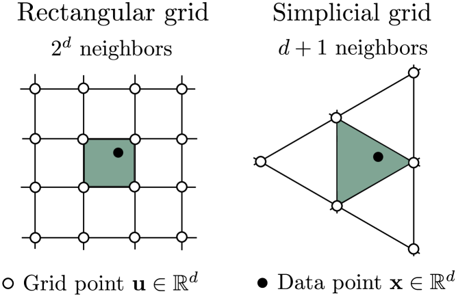
Figure 1: Comparison of the number of grid points required in SKI (Wilson & Nickisch, 2015) against our method. SKI requires exponentially more number of grid points due to its dense lattice construction. Simplex-GP on the other hand can get away with only a sparse set of points on the permutohedral lattice.

SKI tiles the data space with a dense rectangular grid of inducing points. By interpolating kernels to the grid, and exploiting structure in the matrices, SKI greatly reduces the computational cost of inference to be only linear in the dataset size and sub-quadratic in the number of grid points. The powerful grid structure of SKI, however, is also its downfall in high dimensional settings, since SKI requires at least $2^{d}$ grid points for a $d$-dimensional dataset. Thus, SKI requires time and memory exponential in the dataset dimensionality, making it unsuitable for datasets with more than $\sim 5$ dimensions. Building on SKI, Gardner et al. (2018b) proposed SKIP, which reuses a one-dimensional grid across all dimensions and builds up low rank approximations to the covariance matrices, reducing inference time to be linear in $n$ as well as $d$. However, even with these improvements, SKIP is limited to $d\sim 10$ to $30$ for large datasets since the method uses memory equivalent to storing $\sim 20\cdot d$ copies of the training dataset, and the low rank approximation can sometimes be limiting.

Dimensionality is not a challenge in GP inference alone. In image filtering, a broad class of non-linear edge-preserving filters including the bilateral filter, non-local means, and other related filters have found growing importance (Aurich & Weule, 1995; Tomasi & Manduchi, 1998; Paris & Durand, 2006). Such filters map a set of vector values ${\{{\bm{\mathbf{y}}}_{i}\}\subseteq\mathbb{R}^{n}}$ (typically the pixel values in an image) to ${\{{\bm{\mathbf{y}}}^{\prime}_{i}\}\subseteq\mathbb{R}^{n}}$ where each ${\bm{\mathbf{y}}}^{\prime}_{i}$ is a Gaussian weighted linear combination of vectors at locations ${\{{\bm{\mathbf{x}}}_{i}\}_{i=1}^{n}\subseteq\mathbb{R}^{d}}$:

$${\bm{\mathbf{y}}}_{i}^{\prime}=\sum_{j=1}^{n}e^{-\left\lVert{\bm{\mathbf{x}}}_{j}-{\bm{\mathbf{x}}}_{i}\right\rVert^{2}}{\bm{\mathbf{y}}}_{j}\leavevmode\nobreak\ ,$$ (1)

which can be rewritten as a matrix-vector product involving a matrix with entries ${(K_{{\bm{\mathbf{X}}},{\bm{\mathbf{X}}}})_{ij}=e^{-\left\lVert{\bm{\mathbf{x}}}_{j}-{\bm{\mathbf{x}}}_{i}\right\rVert^{2}}}$.

The naive implementation is computationally expensive to be run on images, and to remedy this, many fast approximations have been developed including the popular permotohedral lattice (Adams et al., 2010), enabling real time filtering rates on images and in fairly high dimensions.

In these seemingly disparate fields of GP inference and high-dimensional Gaussian filtering, we find complementary strengths. On one hand, GP inference is made scalable by structure-exploiting algebra through the SKI framework, but is limited by the exponential scaling in dimension. On the other hand, high-dimensional Gaussian filtering relies on a similar sparse linear combination of the neighborhood, and makes scaling with respect to dimension favorable by embedding points onto the permutohedral lattice. Our work combines these strengths into an inference algorithm for Gaussian processes by computing 1 over the permutohedral lattice using matrix-vector multiplications.

Inspired by the connection between image filtering and kernel methods, we develop Simplex-GP, an interpolation-based scalable Gaussian process approximation method that leverages advances in high-dimensional image filtering. Instead of using a dense cubic grid as in SKI, we employ a sparse simplicial lattice. In the SKI framework, observations must be interpolated to their neighbors in the lattice. Crucially, while each data point in the cubic lattice has $2^{d}$ neighbors, each point in a simplicial lattice has only $d+1$ neighbors, as illustrated in Figure 1. This fact allows us to use exponentially fewer inducing points than in SKI, and perform GP inference in time $\mathcal{O}\left(d^{2}(n+m)\right)$ and $\mathcal{O}\left(dm\right)$ memory where $m$ is the number of inducing points.

Our key contributions are summarized below:

• Drawing parallels between image filtering and Gaussian process inference, we develop a novel kernel interpolation scheme using the permutohedral lattice (Adams et al., 2010). Our method can perform GP inference in $\mathcal{O}\left(n\cdot d^{2}\right)$ time, exponentially faster than SKI which requires $\mathcal{O}\left(n\cdot 2^{d}\right)$ time, for a set of $n$ $d$-dimensional inputs.

• To allow optimization of the marginal likelihood with respect to kernel hyperparameters using off-the-shelf automatic differentiation-based optimizers (Paszke et al., 2019), we show how gradients can also be efficiently formulated as filtering operations on the lattice alone.

• We extend the permutohedral lattice to include filtering with respect to general stationary kernels such as the Matérn kernel (Rasmussen & Williams, 2005).

• We provide efficient CPU and CUDA accelerated implementations of permutohedral lattice filtering at u.perhapsbay.es/simplex-gp-code. Our implementations are compatible with GPyTorch (Gardner et al., 2018a), making them amenable for easy use with other numerical methods.

In summary, our method Simplex-GP provides a scalable extension to the SKI framework, which alleviates both the low-dimensional limitations of KISS-GP (Wilson & Nickisch, 2015), and high-memory requirements of SKIP (Gardner et al., 2018b), by instead packing the inputs into a more efficient lattice. This is followed by significant performance gains over SKIP, reducing the performance gap to exact Gaussian processes.

2 Gaussian Processes

By expressing priors over functions, GPs allow us to build flexible non-parametric function approximators that can learn structure in data through covariance functions (Rasmussen & Williams, 2005). In a typical regression setting, for a dataset $\mathcal{D}$ of size $n$, we model the relationship between inputs (predictors) ${{\bm{\mathbf{X}}}=\left[{\bm{\mathbf{x}}}_{1},{\bm{\mathbf{x}}}_{2},\dots,{\bm{\mathbf{x}}}_{n}\right]\in\mathbb{R}^{n\times d}}$ and corresponding outputs ${{\bm{\mathbf{y}}}=\left[y({\bm{\mathbf{x}}}_{1}),y({\bm{\mathbf{x}}}_{2}),\dots,y({\bm{\mathbf{x}}}_{n})\right]^{\top}\in\mathbb{R}^{n}}$ using a Gaussian process prior, ${{\bm{\mathbf{f}}}=\left[f({\bm{\mathbf{x}}}_{1}),f({\bm{\mathbf{x}}}_{2}),\dots,f({\bm{\mathbf{x}}}_{n})\right]^{\top}\sim\mathcal{GP}\left({\bm{\mathbf{\mu}}}_{{\bm{\mathbf{X}}}},K_{{\bm{\mathbf{X}}},{\bm{\mathbf{X}}}}\right)}$, determined by a mean vector ${({\bm{\mathbf{\mu}}}_{{\bm{\mathbf{X}}}})_{i}={\bm{\mathbf{\mu}}}({\bm{\mathbf{x}}}_{i})}$ and a covariance matrix ${(K_{{\bm{\mathbf{X}}},{\bm{\mathbf{X}}}})_{ij}=k_{\theta}({\bm{\mathbf{x}}}_{i},{\bm{\mathbf{x}}}_{j})}$. The kernel function $k_{\theta}$ is parametrized by $\theta$. The observation likelihood is assumed to be input-independent Gaussian additive noise, i.e. ${y({\bm{\mathbf{x}}})\mid f({\bm{\mathbf{x}}})\sim\mathcal{N}\left(f({\bm{\mathbf{x}}}),\sigma^{2}\right)}$ with variance $\sigma^{2}$.

In maximum likelihood inference, we compute the posterior over functions ${p(f\mid\mathcal{D},\theta,\sigma^{2})}$ using parameters ${\{\theta,\sigma^{2}\}}$ that maximize the marginal $\log$-likelihood ${\log{p({\bm{\mathbf{y}}}\mid{\bm{\mathbf{X}}})}}$. For the chosen prior and likelihood pair, the predictive distribution at $n_{\star}$ test inputs is a multivariate Gaussian $\mathcal{N}\left(\mathbb{E}\left[{\bm{\mathbf{f}}}_{\star}\right],\mathrm{cov}\left({\bm{\mathbf{f}}}_{\star}\right)\right)$ where,

$$\mathbb{E}\left[{\bm{\mathbf{f}}}_{\star}\right]= \leavevmode\nobreak\ {\bm{\mathbf{\mu}}}_{{\bm{\mathbf{X}}}_{\star}}+K_{{\bm{\mathbf{X}}}_{\star},{\bm{\mathbf{X}}}}\left[K_{{\bm{\mathbf{X}}},{\bm{\mathbf{X}}}}+\sigma^{2}{\bm{\mathbf{I}}}\right]^{-1}{\bm{\mathbf{y}}},$$ (2)

$$\begin{split}\mathrm{cov}\left({\bm{\mathbf{f}}}_{\star}\right)=&\leavevmode\nobreak\ K_{{\bm{\mathbf{X}}}_{\star},{\bm{\mathbf{X}}}_{\star}}-\\ &\leavevmode\nobreak\ K_{{\bm{\mathbf{X}}}_{\star},{\bm{\mathbf{X}}}}\left[K_{{\bm{\mathbf{X}}},{\bm{\mathbf{X}}}}+\sigma^{2}{\bm{\mathbf{I}}}\right]^{-1}K_{{\bm{\mathbf{X}}},{\bm{\mathbf{X}}}_{\star}}.\end{split}$$ (3)

The marginal $\log$-likelihood (MLL) is given by,

$$\begin{split}\log{p({\bm{\mathbf{y}}}\mid{\bm{\mathbf{X}}})}\propto&-\tfrac{1}{2}{\bm{\mathbf{y}}}^{\top}\left(K_{{\bm{\mathbf{X}}},{\bm{\mathbf{X}}}}+\sigma^{2}{\bm{\mathbf{I}}}\right)^{-1}{\bm{\mathbf{y}}}\\ &-\tfrac{1}{2}\log{\left\lvert K_{{\bm{\mathbf{X}}},{\bm{\mathbf{X}}}}+\sigma^{2}{\bm{\mathbf{I}}}\right\rvert}.\end{split}$$ (4)

Owing to inverse and determinant computations in 2, 3 and 4, naive inference takes $\mathcal{O}\left(n^{3}\right)$ compute and $\mathcal{O}\left(n^{2}\right)$ storage, which is prohibitively expensive for large $n$. Modern state-of-the-art and scalable implementations of GP regression (Gardner et al., 2018a; Matthews et al., 2017), however, rely on Krylov subspace methods like conjugate gradients (CG) (Golub & Loan, 1996); more recently, Wang et al. (2019) demonstrated that exact Gaussian processes can be scaled to more than a million input data using such methods. These methods depend only on Matrix Vector Multiplications (MVMs): ${\mathbf{v}\mapsto K_{{\bm{\mathbf{X}}},{\bm{\mathbf{X}}}}\mathbf{v}}$ rather than computing the elements of $K_{{\bm{\mathbf{X}}},{\bm{\mathbf{X}}}}$ itself. The complexity of one inference step is reduced to $\mathcal{O}\left(pn^{2}\right)$ for $p$ CG iterations, where typically ${p\ll n}$ suffices in practice.

Alternatively, inducing point methods (Candela & Rasmussen, 2005; Titsias, 2009; Hensman et al., 2013, 2015b) have been introduced as a scalable approximation to exact GPs. A set of $m$ inducing points or pseudo-inputs are introduced as parameters, with usual GP inference built on top of these points. One-step inference costs only $\mathcal{O}\left(m^{2}n+m^{3}\right)$ compute and $\mathcal{O}\left(m^{2}+mn\right)$ storage, but the cross-covariance term corresponding to the $m^{2}n$ factor can still be costly, limiting $m\ll n$.

2.1 Structured Kernel Interpolation

Wilson & Nickisch (2015) show that using Structured Kernel Interpolation (SKI) to introduce algebraic structure, we can use extremely high number of inducing points, irrespective of the nature of the input space. Using simple sparse interpolation schemes (e.g. inverse distance weighting or spline interpolation), one can accelerate the computations required for computing the covariance matrices via KISS-GP (Wilson & Nickisch, 2015; Wilson et al., 2015).

Given a set of $m$ inducing points ${{\bm{\mathbf{U}}}=[{\bm{\mathbf{u}}}_{1},{\bm{\mathbf{u}}}_{2},\dots,{\bm{\mathbf{u}}}_{m}]}$, Wilson & Nickisch (2015) propose a general approximation to the cross-covariance kernel matrix ${K_{{\bm{\mathbf{X}}},{\bm{\mathbf{U}}}}\in\mathbb{R}^{n\times m}}$ as ${\widetilde{K}_{{\bm{\mathbf{X}}},{\bm{\mathbf{U}}}}=W_{\bm{\mathbf{X}}}K_{{\bm{\mathbf{U}}},{\bm{\mathbf{U}}}}}$, where ${W_{\bm{\mathbf{X}}}\in\mathbb{R}^{n\times m}}$ describe the interpolation weights. Subsequently, one can plug this into the subset of regressors (SoR) (Silverman, 1985; Candela & Rasmussen, 2005) formulation, and prior covariance is approximated by 5.

$$K_{{\bm{\mathbf{X}}},{\bm{\mathbf{X}}}}\approx W_{\bm{\mathbf{X}}}K_{{\bm{\mathbf{U}}},{\bm{\mathbf{U}}}}W_{\bm{\mathbf{X}}}^{\top}\triangleq\widetilde{K}_{{\bm{\mathbf{X}}},{\bm{\mathbf{X}}}}\leavevmode\nobreak\ .$$ (5)

The SKI framework now allows one to posit efficient structures for the inducing points irrespective of the nature of the input points, such that the matrix $K_{{\bm{\mathbf{U}}},{\bm{\mathbf{U}}}}$ inherits efficient computation. For instance, placing the inducing points on a rectilinear grid allows one to exploit Toeplitz or Kronecker algebra (Wilson & Nickisch, 2015). Further, by using local interpolations (e.g. inverse distance weighting, or spline interpolation in Wilson & Nickisch (2015)) instead of global GP interpolations, the sparsity induced in the weights matrix $W_{\bm{\mathbf{X}}}$ greatly improves scalability by allowing $m\gg n$. The inference proceeds by plugging ${\widetilde{K}_{{\bm{\mathbf{X}}},{\bm{\mathbf{X}}}}+\sigma^{2}{\bm{\mathbf{I}}}}$ into a conjugate gradients and an eigenvalue solver for $\log$-determinant computations. This method, termed as KISS-GP, is also amenable to general Krylov subspace methods (Golub & Loan, 1996; Gardner et al., 2018a).

When exploiting Toeplitz structure in the inducing points, KISS-GP requires $\mathcal{O}\left(n2^{d}+m\log{m}\right)$ compute and $\mathcal{O}\left(n+m\right)$ storage. When exploiting Kronecker structure in the inducing points, KISS-GP requires $\mathcal{O}\left(n2^{d}+dm^{1+1/d}\right)$ compute and $\mathcal{O}\left(n+dm^{2/d}\right)$ storage. The number of inducing points $m$, however, grow exponentially in number with the dimension, as a consequence of being embedded in a rectangular grid, limiting the application to small dimensions. Within the SKI framework, Gardner et al. (2018b) instead propose SKIP, which provides an efficient application of MVMs to stationary kernels that can be decomposed as Hadamard products across dimensions. Low rank approximations in SKIP, however, can reduce performance.

Our work lies within the SKI framework, and provides a scalable approach which alleviates both the low-dimensional limitations of KISS-GP (Wilson et al., 2015), and high-memory requirements of SKIP (Gardner et al., 2018b), by instead packing the inputs into a more efficient lattice, while performing significantly better on our benchmark datasets.

3 Bilateral Filtering

Gaussian processes aside, bilateral filtering is a popular method in the image processing community (Aurich & Weule, 1995; Tomasi & Manduchi, 1998). The Gaussian blur filter is a common tool in signal processing, computer vision, computational photography, and elsewhere for smoothing out noise, irregularities, and unwanted high frequency information. In the image domain especially, signals have hard discontinuities such as those caused by occlusion. Special edge-preserving filters have been developed to smooth signals while preserving meaningful edges and boundaries, the most popular of which is the bilateral filter (Paris & Durand, 2006).

Extending the Gaussian blur, the bilateral filter is a nonlinear filter that is Gaussian in both spatial distance and the RGB difference in intensity. Mathematically, the blurred pixels have the value

$${\bm{\mathbf{v}}}^{\prime}_{i}=\sum_{i}\left(e^{-\left\lVert{\bm{\mathbf{p}}}_{i}-{\bm{\mathbf{p}}}_{j}\right\rVert^{2}/2\sigma_{p}^{2}-\left\lVert{\bm{\mathbf{v}}}_{i}-{\bm{\mathbf{v}}}_{j}\right\rVert^{2}/2\sigma_{v}^{2}}\right){\bm{\mathbf{v}}}_{j}\leavevmode\nobreak\ ,$$ (6)

where ${\bm{\mathbf{v}}}_{i}\in\mathbb{R}^{3}$ is a vector of the RGB pixel intensities for a given pixel index $i$ and ${\bm{\mathbf{p}}}_{i}\in\mathbb{Z}^{2}$ is the horizontal and vertical coordinates of the pixel on the grid.

The bilateral filter has proven effective in many low level image tasks such as haze removal (Zhu et al., 2015), contrast adjustment, detail enhancement (Fattal et al., 2007), image matting, depth upsampling (Barron & Poole, 2016), and even semantic segmentation (Krähenbühl & Koltun, 2011). A variant of the bilateral filter known as the joint bilateral filter allows for blurring of an image ${\bm{\mathbf{v}}}$ while respecting the edges in a second reference image ${\bm{\mathbf{u}}}$, and in general concatenating ${{\bm{\mathbf{x}}}:=\mathrm{Concat}({\bm{\mathbf{p}}}/\sigma_{p},{\bm{\mathbf{u}}}/\sigma_{u})}$ we can write the operation more abstractly as 1.

A major challenge with bilateral filtering is the $\mathcal{O}\left(n^{2}\right)$ computation cost which is extremely costly for images. Various approaches have been proposed in the literature to accelerate the computation such as the Fast Gauss Transform (Greengard & Strain, 1991), Gaussian KD-tree (Adams et al., 2009), Guided Filter (He et al., 2010), and the permutohedral lattice (Adams et al., 2010). Due its favorable $O(nd^{2})$ scaling and the generality of the method, the permutohedral lattice has been the method of choice for downstream applications (Krähenbühl & Koltun, 2011; Kiefel et al., 2014; Su et al., 2018).

3.1 GP Inference with the RBF Kernel is Equivalent to Bilateral Filtering

Efficient inference in Gaussian processes depends directly on having an efficient way to perform matrix vector multiplications using the kernel matrix $K_{{\bm{\mathbf{X}}},{\bm{\mathbf{X}}}}$. For RBF kernels, after normalizing by lengthscale $x_{i}\mapsto x_{i}/\ell$, this matrix is precisely the same as the one that defines bilateral filtering, ${k({\bm{\mathbf{x}}}_{i},{\bm{\mathbf{x}}}_{j})=e^{-\tfrac{1}{2}\left\lVert{\bm{\mathbf{x}}}_{j}-{\bm{\mathbf{x}}}_{i}\right\rVert^{2}}}$. In both cases, these vectors can lie off the grid because of the color intensity in bilateral filter and naturally ungridded data for GPs. In this general framing, methods that are used to accelerate image filtering, can also be used to accelerate GP inference (and vice- versa).

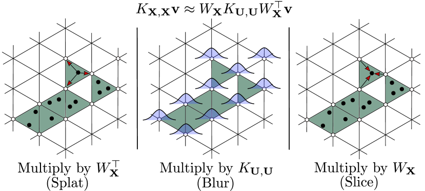
Figure 2: Filtering using the permutohedral lattice involves three stages - Splat, Blur, and Slice. The usual convolutions required for Blur are wrapped by a projection onto the lattice via barycentric interpolation (Splat), and finally resampling the lattice at input locations for the filtering output (Slice). This is equivalent to the SKI decomposition, but with a different grid.

The SKI and the permutohedral lattice filtering, despite arising from separate communities, are in fact closely related. In the SKI decomposition, ${K_{{\bm{\mathbf{X}}},{\bm{\mathbf{X}}}}\approx W_{\bm{\mathbf{X}}}K_{{\bm{\mathbf{U}}},{\bm{\mathbf{U}}}}W_{\bm{\mathbf{X}}}^{\top}}$ the linear operations ${\bm{\mathbf{v}}}\mapsto W_{\bm{\mathbf{X}}}^{\top}{\bm{\mathbf{v}}}$, ${\bm{\mathbf{w}}}\mapsto K_{{\bm{\mathbf{U}}},{\bm{\mathbf{U}}}}{\bm{\mathbf{w}}}$ and ${\bm{\mathbf{v}}}^{\prime}\mapsto W_{\bm{\mathbf{X}}}{\bm{\mathbf{v}}}^{\prime}$ map precisely to the Splat, Blur, and Slice stages respectively of filtering with the permutohedral lattice (Adams et al., 2010). Splat interpolates the values onto the lattice points, Blur applies the filter on the lattice, and Slice interpolates back to the original locations. SKI uses linear interpolation to a cubic lattice, whereas the permutohedral filtering uses barycentric interpolation to a simplicial lattice. While SKI stores values densely in the lattice with dense arrays, the permutohedral lattice stores values sparsely using a hash table. With SKI, the cubic lattice ${K_{{\bm{\mathbf{U}}},{\bm{\mathbf{U}}}}=K_{{\bm{\mathbf{U}}}_{1},{\bm{\mathbf{U}}}_{1}}\otimes\cdots\otimes K_{{\bm{\mathbf{U}}}_{d},{\bm{\mathbf{U}}}_{d}}}$ induces Kronecker structure to enable efficient computation, whereas with the permutohedral lattice the computation splits over the (non- orthogonal) lattice directions. We visualize this correspondence in Figure 2, and review permutohedral lattice filtering in the context of kernel interpolation.

3.2 Permutohedral Lattice

Grids have been used in the past not just for scalable GPs but also bilateral filtering (Chen et al., 2007). An important distinction from prior approaches, Adams et al. (2010) discovered that the key to avoiding the curse of dimensionality is in using a simplicial lattice rather than a cubic one, which they term a permutohedral lattice.

The permutohedral lattice is a higher-dimensional generalization of the hexagonal lattice built from triangles in $\mathbb{R}^{2}$ to simplices in $\mathbb{R}^{d}$. Each of these simplicies are the same, and can best understood as permutations of a canonical simplex, with vertices ${{\bm{\mathbf{s}}}_{0},{\bm{\mathbf{s}}}_{1},\dots,{\bm{\mathbf{s}}}_{d}}$ given by,

$${\bm{\mathbf{s}}}_{k}=[\leavevmode\nobreak\ \underbrace{k,\dots,k}_{d+1-k},\underbrace{k-(d+1),\dots,k-(d+1)}_{k}\leavevmode\nobreak\ ]\leavevmode\nobreak\ .$$ (7)

These vertices form a basis of a $d$ dimensional hyperplane $H_{d}$. See Baek et al. (2012) for a detailed exposition on the theoretical properties of the permutohedral lattice. Following the terminology in Adams et al. (2010), filtering using the permutohedral lattice involves three operations – Splat, Blur, and Slice. In essence, the filtering is carried out by the Blur operation. The Splat and Slice operations provide the mapping of the position vectors, between the input space and the lattice embedding space. Figure 2 illustrates operations on the permutohedral lattice for two-dimensional inputs.

Splat

The input vectors ${\bm{\mathbf{x}}}$ are first embedded into the subspace defined by $H_{d}$. While the linear map can be constructed directly using the basis defined by 7, one can more efficiently compute the embedding in linear time, i.e. $\mathcal{O}\left(d\right)$, by instead using a more efficient triangular basis, which we denote by ${\bm{\mathbf{E}}}$.

Surrounding the embedded point, one can find the enclosing simplex and its vertices by a rounding algorithm and comparison to a canonical simplex in a total $\mathcal{O}\left(d^{2}\right)$ time (Conway & Sloane, 1988). These vertices serve as the inducing points for Simplex-GP to which the value $v$ is projected.

Given the bounding vertices ${\bm{\mathbf{s}}}_{k}$ of the given point inside the simplex (of which there are only $d+1$ rather than $2^{d}$ for a cubic lattice), barycentric interpolation weights $w_{k}$ are computed based on the proximity to each of the vertices $\left\lVert{\bm{\mathbf{x}}}-{\bm{\mathbf{s}}}_{k}\right\rVert$. These weights are the $d+1$ nonzero values in the matrix in each row $W_{\bm{\mathbf{x}}}$ of $W_{\bm{\mathbf{X}}}$, giving it the sparse structure similar to the interpolation matrix in KISS-GP. These inducing point vertices are stored in a hash table along with the splatted values $W_{\bm{\mathbf{X}}}^{\top}{\bm{\mathbf{v}}}$. Unlike KISS-GP, the lattice vertices (inducing points) which do not border any point ${\bm{\mathbf{x}}}$ are not computed or stored.

The amortized hash-table lookup compute is then $\mathcal{O}\left(d\right)$. For a total of $m$ hashtable entries corresponding to the generated lattice points (inducing points), the total storage needed is $\mathcal{O}\left(md\right)$, where $m$ itself is loosely upper- bounded by $\mathcal{O}\left(nd\right)$. We empirically demonstrate the significant storage gains due to embedding into the permutohedral lattice. Each input ${\bm{\mathbf{x}}}$ is now represented as a barycentric interpolation of the lattice points ${\bm{\mathbf{u}}}$ in the enclosing simplex.

Blur

Having constructed the lattice, the Blur operation is simply a convolution with the neighbors in the lattice using an appropriately-sized stencil across each direction in the lattice sequentially ($d+1$ in total). There are $\mathcal{O}\left(d\right)$ neighbors to lookup, and each lookup in the hashtable requires $\mathcal{O}\left(d\right)$ time. Therefore, each blur step can be completed in $\mathcal{O}\left(d^{2}\right)$ time. As an example, a Gaussian blur can be implemented by convolving with the binomial stencil ${\left[.5,1,.5\right]}$ across each direction in the lattice. In Section 4.1, we describe a general approach to build stencils for any stationary kernel in Gaussian processes. We note however that in principle lattice points could be added to the hash table in the blurring along one axis that could affect the subsequent blur steps along the other directions; however, like (Adams et al., 2010) we ignore this second order effect and keep the number of inducing points fixed during the filtering operation.

Slice

The Slice operation resamples the values back at the input location using barycentric interpolation weights as before (the transpose of the sparse matrix $W_{X}^{\top}$). By caching the barycentric weights for each generated lattice point during splatting, we can avoid any redundant computations, and recover the values in $\mathcal{O}\left(d\right)$ time. A complete scan over all the inputs will therefore take $\mathcal{O}\left(nd\right)$.

In summary, the entire algorithm for filtering using the permutohedral lattice requires $\mathcal{O}\left(d^{2}(n+m)\right)$ compute, and $\mathcal{O}\left(dm\right)$ storage.

4 Simplex Gaussian Processes

We have established in Section 3.1 that bilateral filtering, and RBF kernel MVMs in GP inference are fundamentally the same. Section 3.2 describes an accelerated approach to high-dimensional Gaussian filtering. Consequently, our proposed inference method, named Simplex Gaussian processes (Simplex-GPs), effectively leverage this connection by replacing the exact MVMs with accelerated bilateral filtering using the permutohedral lattice. In summary, the SKI decomposition 5, and the corresponding bilateral filtering stages are annotated in 8. The computational complexity of inference in Simplex-GPs is listed alongside other GP inference methods in Table 1.

$$K_{{\bm{\mathbf{X}}},{\bm{\mathbf{X}}}}\approx\underbrace{W_{{\bm{\mathbf{X}}}}}_{\mathrm{Slice}}\underbrace{K_{{\bm{\mathbf{U}}},{\bm{\mathbf{U}}}}}_{\mathrm{Blur}}\underbrace{W_{{\bm{\mathbf{X}}}}^{\top}}_{\mathrm{Splat}}\leavevmode\nobreak\ .$$ (8)

Notably, in this decomposition, only the blur matrix $K_{{\bm{\mathbf{U}}},{\bm{\mathbf{U}}}}$ depends on the choice of the stationary kernel used to model the Gaussian process prior. The Splat $W_{{\bm{\mathbf{X}}}}^{\top}$ and Slice $W_{{\bm{\mathbf{X}}}}$ matrices remain the same.

Without further changes, the bilateral filtering on the permutohedral lattice is only equivalent to a MVM with RBF kernel. However, we may wish to use other stationary kernels with GP inference. Stationary kernels that depend only on the difference between the points, ${\tau=\lvert{\bm{\mathbf{u}}}_{i}-{\bm{\mathbf{u}}}_{j}\rvert}$, which includes a broad class of kernels, including the RBF kernel and the Matérn kernel (Rasmussen & Williams, 2005). To adapt our method to another stationary kernel like, we simply have to compute an appropriate stencil of coefficients to build a discrete approximation of the non-Gaussian kernel $k(\tau)$. We now develop this approximation.

Table 1: Time complexities for MVM used during Gaussian process inference. $n$ is the number of inputs, $m$ is the number of inducing points, and $r$ is the rank used in the SKIP approximation (typically between $20$ and $100$).

Method Time Complexity of one MVM Exact $\mathcal{O}\left(n^{2}\right)$ KISS-GP (Kronecker) $\mathcal{O}\left(n2^{d}\right)$ SKIP $\mathcal{O}\left(rnd\right)$ Simplex-GP $\mathcal{O}\left(nd^{2}\right)$

4.1 Discretizing Generic Stationary Kernels

We can compute the discretized stencil coefficients by evaluating the kernel along the lattice points. Let ${\bm{\mathbf{x}}}^{\prime}$ be $i$ points apart from ${\bm{\mathbf{x}}}$ along a given lattice direction ${\bm{\mathbf{s}}}_{k}$ such that ${{\bm{\mathbf{x}}}^{\prime}={\bm{\mathbf{x}}}+i{\bm{\mathbf{s}}}_{k}}$. For a stationary kernel $k$, we then have $k({\bm{\mathbf{x}}},{\bm{\mathbf{x}}}^{\prime})=k(\left\lVert{\bm{\mathbf{x}}}-{\bm{\mathbf{x}}}^{\prime}\right\rVert^{2})=k(is)$ where ${s:=\left\lVert{\bm{\mathbf{s}}}_{k}\right\rVert}$ is the size of the lattice spacing. We can approximate $k({\bm{\mathbf{x}}},\cdot)$ by only considering the points ${\bm{\mathbf{x}}}^{\prime}$ that lie within $i$ spaces apart with $i=-r,...,r$. We can then choose $r$ based on how quickly the tails of $k$ decay in order to reach a desired error threshold. Even with a fixed number of evenly spaced points at which to evaluate the kernel, there is an additional free parameter $s$, corresponding to the spacing between points, which we must determine in order to maximize the accuracy of our stencil for $k$.

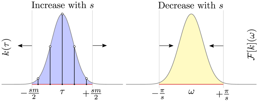
Figure 3: Increasing the coverage in the spatial domain $\tau$ (left), reduces the coverage in Fourier domain $\omega$ (right), monotonically due to aliasing. Finding a good spacing $s$ for the discretization amounts to balancing the coverage defined by 9. Each vertical stick in the spatial domain covers a region $[-s/2,s/2]$ around itself.

When choosing this spacing, we must balance the coverage of the underlying kernel function in both the spatial and frequency domains (Birchfield, 2016). For a fixed number of points, increasing the spacing will cover a larger fraction of the kernel function in the spatial domain, but a reduce coverage of the function in the Fourier domain due to aliasing. Given $m=2r+1$ discretization points with $r\geq 0$, our stencil in the spatial domain covers the interval $[-sm/2,sm/2]$. Since the points are spaced $s$ apart, the Nyquist frequency is ${f_{\text{ny}}=1/(2s)}$ or ${\omega_{\text{ny}}=2\pi f_{\text{ny}}=\pi/s}$ in radians. Therefore, matching coverage of $k$ in both domains requires that

$$\frac{\int_{-sm/2}^{sm/2}k(\tau)d\tau}{\int_{-\infty}^{\infty}k(\tau)d\tau}=\frac{\int_{-\pi/s}^{\pi/s}\mathcal{F}[k](\omega)d\omega}{\int_{-\infty}^{\infty}\mathcal{F}[k](\omega)d\omega}\leavevmode\nobreak\ .$$ (9)

Since both $k(\tau)$ and $\mathcal{F}[k](\omega)$ are strictly positive, the left-hand-side increases monotonically with $s$ while the right-hand-side decreases monotonically with $s$. Therefore, the intersection can be found with binary search. The value of $s$ at this intersection is then the optimal spacing for kernel $k$ given $m=2r+1$ discretization points according to our coverage criterion. Although the Fourier transforms of most stationary kernels are known analytically, we use the discrete FFT and numerical integration in our procedure to allow us to quickly adapt our method to new stationary kernels.

4.2 Efficient Gradients Using the Permutohedral Lattice

To perform maximum likelihood GP inference, we must optimize the marginal $\log$-likelihood given in 4 through gradient-based optimization. By relying on the BBMM method proposed in Gardner et al. (2018a), we need only a black-box function to compute kernel matrix MVMs and the derivative of the black-box function MVMs with respect to the kernel inputs. To remain computationally efficient, we must have efficient routines for both the MVM and its derivative. Here we show how to use the permutohedral lattice to also approximate the derivative of our MVM with respect to the input points.

Given a stationary kernel ${k:\mathbb{R}^{d}\times\mathbb{R}^{d}\to\mathbb{R}}$, vectors ${\{{\bm{\mathbf{v}}}_{i}\}\subseteq\mathbb{R}^{n}}$ and ${\{{\bm{\mathbf{x}}}_{i}\}\subseteq\mathbb{R}^{d}}$, we have that,

$${\bm{\mathbf{u}}}_{i} :=\sum_{j}k(\mathbf{x}_{i},\mathbf{x}_{j}){\bm{\mathbf{v}}}_{j}=\sum_{j}k(d_{ij}^{2}){\bm{\mathbf{v}}}_{j}\leavevmode\nobreak\ ,$$ (10)

where $d_{ij}^{2}=\left\lVert{\bm{\mathbf{x}}}_{i}-{\bm{\mathbf{x}}}_{j}\right\rVert^{2}$.

The Jacobian vector products for this operation are: ${\frac{\partial L}{\partial\mathbf{x}_{n}}=\sum_{i,j}\frac{\partial L}{\partial{\bm{\mathbf{u}}}_{i}}\frac{\partial k(d^{2}_{ij})}{\partial\mathbf{x}_{n}}{\bm{\mathbf{v}}}_{j}}$. Noting that ${\frac{\partial d^{2}_{ij}}{\partial\mathbf{x}_{n}}=2(\mathbf{x}_{i}-\mathbf{x}_{j})(\delta_{in}-\delta_{jn})}$ where $\delta$ is the Kronecker delta, we can rewrite the gradients as:

$$\frac{\partial L}{\partial\mathbf{x}_{n}}=2\sum_{i,j}\frac{\partial L}{\partial{\bm{\mathbf{u}}}_{i}}k^{\prime}(d^{2}_{ij})(\mathbf{x}_{i}-\mathbf{x}_{j})(\delta_{in}-\delta_{jn})\leavevmode\nobreak\ ,$$ (11)

where $k^{\prime}$ is the derivative with respect to $d^{2}$. As pointed out in Krähenbühl & Koltun (2011), even with the Gaussian filter $k^{\prime}=k$, the computation does not seem to admit an implementation in terms of lattice filtering with the kernel. However, by splitting up the terms we can rewrite the sum as a lattice filtering of the gradients and outputs using the $k^{\prime}$ kernel where either the input our output of the filter is elementwise multiplied by $\mathbf{x}$. Abbreviating ${k_{ij}^{\prime}:=k^{\prime}(d^{2}_{ij})}$ and ${{\bm{\mathbf{g}}}_{i}:=\frac{\partial L}{\partial{\bm{\mathbf{u}}}_{i}}}$, we have

$$\begin{split}\frac{\partial L}{\partial\mathbf{x}_{n}}=2\sum_{j}\big{[}{\bm{\mathbf{v}}}_{n}k_{nj}^{\prime}\mathbf{x}_{j}{\bm{\mathbf{g}}}_{j}-v_{n}\mathbf{x}_{n}k_{nj}^{\prime}{\bm{\mathbf{g}}}_{j}\\ +{\bm{\mathbf{g}}}_{n}k_{nj}^{\prime}\mathbf{x}_{j}{\bm{\mathbf{v}}}_{j}-{\bm{\mathbf{g}}}_{n}\mathbf{x}_{n}k_{nj}^{\prime}{\bm{\mathbf{v}}}_{j}\big{]}.\end{split}$$ (12)

Using the automatic method for determining the filter stencil, we can then evaluate this expression using a single lattice filtering call with the kernel $k^{\prime}$ on the input,

$$V=\mathrm{Concat}([\mathbf{x}\odot{\bm{\mathbf{g}}},-{\bm{\mathbf{g}}},\mathbf{x}\odot{\bm{\mathbf{v}}},-{\bm{\mathbf{v}}}])\leavevmode\nobreak\ ,$$ (13)

where $\odot$ is elementwise multiplication. This way of rewriting the gradients allows us reuse our filtering implementation to compute the gradients of our MVMs efficiently.

5 Experiments

Table 2: Standardized test root mean square error (RMSE) on various large-scale UCI regression datasets, averaged over 3 trials with two standard deviations. We use a $512$ inducing points for SGPR, and $100$ per dimension for SKIP. We were not able to run SKIP on our Titan RTX GPU (24GB) for the Houseelectric dataset, which we denote by Out of Memory (OOM). Numbers for Exact GP are taken from Wang et al. (2019). Best performing scalable GP methods are shown in bold.

Test RMSE Test NLL Dataset Exact GP SGPR SKIP Simplex-GP Exact GP SGPR SKIP Simplex-GP Houseelectric $0.054\pm 0.000$ $\mathbf{0.067}\pm 0.002$ OOM $0.079\pm 0.002$ $-0.207\pm 0.001$ $\mathbf{-1.242}\pm 0.057$ OOM $0.756\pm 0.075$ Precipitation $0.937\pm 0.000$ $1.033\pm 0.004$ $1.032\pm 0.001$ $\mathbf{0.939}\pm 0.001$ $\mathrm{-}$ $1.437\pm 0.006$ $1.451\pm 0.001$ $\mathbf{1.397}\pm 0.001$ Keggdirected $0.083\pm 0.001$ $0.380\pm 0.018$ $0.487\pm 0.005$ $\mathbf{0.095}\pm 0.002$ $-0.838\pm 0.031$ $0.985\pm 0.007$ $0.996\pm 0.013$ $\mathbf{0.797}\pm 0.031$ Protein $0.511\pm 0.009$ $0.579\pm 0.003$ $0.817\pm 0.012$ $\mathbf{0.571}\pm 0.003$ $0.960\pm 0.003$ $\mathbf{0.982}\pm 0.059$ $1.213\pm 0.020$ $1.406\pm 0.048$ Elevators $0.399\pm 0.011$ $\mathbf{0.356}\pm 0.006$ $0.447\pm 0.037$ $0.510\pm 0.018$ $0.626\pm 0.043$ $1.031\pm 0.230$ $\mathbf{0.869}\pm 0.074$ $1.600\pm 0.020$

In our experiments, we establish that (i) our proposed discretization scheme to approximate a continuous stationary kernel has low error, (ii) leveraging the permutohedral lattice allows us to operate on large scale datasets with over a million data points without demanding significant runtime and memory requirements unlike other methods, and (iii) our method closes the performance gap of SKI methods relative to exact Gaussian processes at a significantly lower computational cost. All code to reproduce results is available at u.perhapsbay.es/simplex-gp-code. All hyper-parameters are documented in Appendix A.

We note that comparisons to KISS-GP are not possible with our evaluation datasets as due to KISS-GP’s exponential scaling with dimension. Within the SKI framework, however, our method Simplex-GP provides a scalable alternative for KISS-GP to dimensions much larger than originally possible, and outperform SKIP in test root mean squared error by a significant margin. Furthermore, on large scale datasets ($n\sim 10^{6}$), we observe that MVMs using the permutohedral lattice are 10x faster than exact MVMs computed with the highly efficient KeOps library (Charlier et al., 2020), and the asymptotics suggest even greater gains on yet larger datasets.

5.1 Evaluating Discretization Error

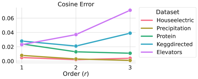
Figure 4: For different sizes of the blur stencil denoted by order $r$, we show the MVM error for the resultant vector $\hat{{\bm{\mathbf{z}}}}$ with Simplex-GPs, as compared to ${\bm{\mathbf{z}}}$ computed with exact GPs using KeOps. We compute the cosine error between the vectors as $1-\frac{\langle{\bm{\mathbf{z}}},\hat{{\bm{\mathbf{z}}}}\rangle}{\left\lVert{\bm{\mathbf{z}}}\right\rVert\left\lVert\hat{{\bm{\mathbf{z}}}}\right\rVert}$. Low values indicate that the two vectors are closely aligned. Importantly, increasing the order of the blur stencil does not always reduce the error, because the truncation in the blur step affects the approximation.

The fundamental unit of computation in Simplex-GP is a matrix-vector multiplication (MVM). It is not feasible to store the complete covariance matrix for many of the large scale datasets we consider. MVMs, however, only require the storage of the resultant vector, and therefore has nimble memory requirements. Consequently, instead of comparing dense covariance matrices between exact GPs and Simplex-GPs on the benchmark datasets, we compute the cosine error of the resultant vector with respect to results from exact GPs via KeOps (Charlier et al., 2020). Figure 4 shows the errors achieved for different sizes of the blur stencil, denoted by order $r$ in Section 4.1.

5.2 Computational Gains from Lattice Sparsity

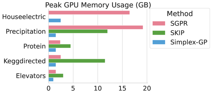
Figure 5: Owing to the significant gains in the number of lattice points generate as reported by Table 3, we see that the approximate peak GPU memory usage of our proposed approximation is significantly lower, allowing operations on large-scale datasets. We were unable to fit the Houselectric dataset with SKIP on one Titan RTX GPU (24GB).

One of the significant advantages of using the permutohedral lattice instead of the Caretesian grid to embed our training inputs is that we can leverage the gains from the efficient packing afforded by the lattice. The permutohedral lattice provably provides the best covering density up to dimension $5$, and is the best known lattice packing up to dimension $20$ (Conway & Sloane, 1988; Baek et al., 2012).

Table 3: Embedding a set of $n$ $d$-dimensional inputs onto a permutohedral lattice generates $m$ lattice points with ${m\leq L:=n\times(d+1)}$ in the worst case. We quantify the sparsity for various UCI regression benchmark datasets as the ratio of lattice points generated to the maximum possible, $m/L$. We observe a significantly fewer number of lattice points generated for our benchmark datasets.

Dataset $n$ $d$ $m$ $m/L$ Houseelectric 2,049,280 11 1,000,190 $0.04$ Precipitation 628,474 3 480 $0.003$ Keggdirected 48,827 20 122,755 $0.12$ Protein 45,730 9 14,715 $0.03$ Elevators 16,599 17 204,761 $0.69$

As noted earlier, each input embedded into the permutohedral lattice can generate at most $d+1$ neighbors. We insert each generated lattice point into a hashtable. Table 3 shows the total number of such lattice points generated on each of standardized benchmark datasets, and compute the ratio to the worst-case scenario, such that a ratio of $1$ corresponds to having generated $L=n\times(d+1)$ lattice points. By storing and manipulating only a sparse lattice, instead of one where all the interior points in the convex hull of the data are generated, the gains from the sparse structure are actually much more than just $m/L$, and exponentially better both in the dimension and the chosen lengthscale.

We observe that the ratios for all datasets are significantly lower than $1$. A ratio closer to one indicates that the input dataset has extremely high variance. Learning in such a scenario would be significantly challenging for any method. As a consequence, we are able to keep the memory usage considerably low, as reported in Figure 5. Figure 6 shows significant speedups for large scale datasets.

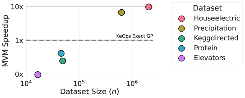
Figure 6: We compare the speed of our Simplex-GP MVMs at order $r=1$ on all benchmark datasets against exact MVMs with KeOps (Charlier et al., 2020), both using one Titan RTX GPU. We achieve up to 10x speedups for large datasets with over $10^{5}$ data points.

5.3 Performance on Benchmark Datasets

We focus on Gaussian process regression, and work with datasets from the UCI repository (Dua & Graff, 2017), which either have large number of training samples, or have a large dimension, to demonstrate the advantages of Simplex-GP.

The data is randomly split into a $4/9\mathrm{-}2/9\mathrm{-}3/9$ train-validation-test split. All datasets are standardized using the training data to have zero mean and unit variance. We report the standardized root mean squared error (RMSE) and the marginal $\log$-likelihood over the test set, with a standard deviation over 3 independent runs. All methods are trained using a learning rate of 0.1 with the Adam optimizer in GPyTorch (Gardner et al., 2018a). As noted in Gardner et al. (2018a), we set the CG error tolerance to $1.0$ during training, but use a lower CG tolerance of $0.01$ during evaluation, which does not significantly hurt performance.

For SGPR (Titsias, 2009), we use the typical value of $m=512$ inducing points, as reported in literature. For SKIP (Gardner et al., 2018b), we use a total of $m=100$ inducing points per dimension, which is significantly larger than originally reported. We were, however, not able to fit inference with SKIP on a single GPU device, even for small values of $m$.

Table 2 reports the standardized test RMSE and the corresponding negative $\log$-likelihoods for our benchmark datasets from the UCI repository. We are able to significantly outperform SKIP (Gardner et al., 2018b), which is one of the more scalable methods within the SKI framework (Wilson et al., 2015). Further, on most datasets, we are able to match or outperform the approximate inducing point method SGPR (Titsias, 2009).

Finally, in Appendix C, we compare the lengthscales learned by Simplex-GPs to those learned by exact GPs (with KeOps) for all our benchmark datasets, noting that the performance of Simplex-GPs is not simply a coincidental artifact of optimization, but provides qualitatively similar automatic relevance determination (ARD).

5.4 Practical Considerations

The Simplex-GP makes use of iterative methods such as conjugate gradients (CG). Conjugate gradients are highly effective for scalable Gaussian processes (Gardner et al., 2018a), but are also sensitive to design decisions and prone to numerical instability. Here we provide guidance to help practitioners seamlessly deploy the Simplex-GP in their own applications. We note many of these considerations are not specific to the Simplex-GP and have broad relevance to CG based GPs.

Conjugate gradients (CG) enable the solution to a rank-$n$ linear system in $p\ll n$ iterations up to machine precision (and exact when $p=n$). In practice, we run CG up to a prescribed error tolerance, or some maximum prescribed value of $p$, whichever is achieved earlier. Using low tolerance or high $p$ can add a significant runtime cost. Wang et al. (2019) recommend that an error tolerance of $10^{-2}$ provides a reasonable trade-off between training time and performance, although this recommendation mostly holds for good RMSE performance rather than good test likelihood. Moreover, this relatively high tolerance can lead to unstable training such that the MLL may not always improve monotonically. We illustrate this pathology in Figure 7 (Appendix B). In addition, early truncations due to a small value of $p$ can introduce bias (Potapczynski et al., 2021). To avoid adverse impact of these pathologies, we rely on early stopping, i.e. we use the RMSE on a held-out validation set to select the best model as a result of the MLL optimization.

Table 4: We compare training runtime on a single epoch of Simplex-GPs with different error tolerance values for conjugate gradients, and observe that the Russian Roulette estimator for randomized CG truncations (RR-CG) (Potapczynski et al., 2021) is able to sustain a much better runtime. This allows us to stabilize training, without compromising the speedup gains from Simplex-GPs by a significant margin. The approximate runtime ranges below represent a the time taken by a single epoch during training in seconds.

Dataset CG $(10^{-2})$ CG $(10^{-4})$ RR-CG $(10^{-8})$ Houseelectric 450-600 2000-4000 950-1200 Precipitation 15-20 20-40 30-40 Keggdirected 40-50 320-340 75-100 Protein 8-10 40-60 15-20 Elevators 18-20 25-30 20-25

For Simplex-GPs, we find that while these numerical instabilities can be alleviated by reducing the CG tolerance to $10^{-4}$ (see Figure 7, Appendix B), there is a significant training slowdown (Table 4). In recent work Potapczynski et al. (2021) propose randomized truncations for bias-free conjugate gradients, termed RR-CG, to remedy these challenges with using CG based inference. In Table 4, we find that RR-CG is useful in avoiding the pathologies while maintaining an acceptable runtime.

The computational gains from Simplex-GPs are a consequence of exploiting the geometry of the data. A proxy for the potential gains in the MVMs is the sparsity ratio of the lattice as in Table 3. Qualitatively, we expect especially large acceleration in datasets where data overlap or large lengthscales lead to a smaller fraction of inducing points $m/L$ over the maximum possible. In general, we expect Simplex-GPs to be especially valuable on large training sets (more than $10^{5}$ points), with moderate input dimensionality (between about $3$ and $20$ dimensional inputs).

6 Conclusion

Our work demonstrates the benefits of cross-pollinating concepts in image filtering with Gaussian process inference. By leveraging the permutohedral lattice for accelerated filtering, we are able to alleviate the curse of dimensionality in Structured Kernel Interpolation. While Simplex-GP results in an asymptotic speedup over standard inference, the runtime constants are large, meaning that this speedup is mostly realized for large datasets. We hope that the promising results here can spur on future work, helping to further broaden the applicability of Simplex-GPs, to higher dimensional problems and a greater range of datasets.

Appendix A Hyperparameters

Table 5 documents all the hyperparameters used for training Simplex-GPs. All kernels use automatic relevance determination (ARD). We find that higher values of $r$ (e.g. $2$ or $3$) do not meaningfully improve the test RMSE performance, but significantly increase the training time.

Table 5: We document all the settings and hyperparameters involved in training Simplex-GPs.

Hyperparameter Value(s) Max. Epochs $100$ Optimizer $\mathrm{Adam}$ Learning Rate $0.1$ CG Train Tolerance $1.0$ CG Eval/Test Tolerance $0.01$ Max. CG Iterations $500$ CG Pre-conditioner Rank $100$ Max. Lanczos Iterations $100$ Kernel Family { $\mathrm{Mat\acute{e}rn}$-3/2, $\mathrm{RBF}$ } Blur Stencil Order ($r$) 1 Min. Likelihood Noise ($\sigma^{2}$) { $10^{-4}$, $10^{-1}$ }

Appendix B Visualizing Training Instabilities

We visualize the training instabilities that arise as a consequence of using a high CG tolerance value. As noted in Section 5.4, we follow the recommendation of Wang et al. (2019), and use a CG tolerance of $1.0$ during training and $0.01$ during validation and test. We find that the train MLL does not improve monotonically, due to lack of CG convergence, often owing to early truncation. This leads to undesirable behavior in the test RMSE as visualized in Figure 7(a).

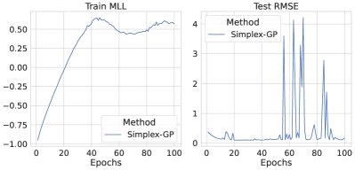
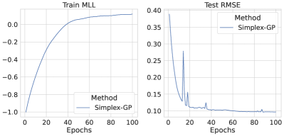
(a)	(b)

Figure 7: We visualize the pathology discussed in Section 5.4, when using conjugate gradients (CG) on the keggdirected dataset. We observe similar behavior for other datasets too. (a) Using a high CG error tolerance of $1.0$ during training leads to non-monotonic improvements in the train marginal $\log$-likelihood (MLL) due to convergence issues in CG. More significantly, this makes the test RMSE curves look unstable. (b) By simply reducing the CG error tolerance to $10^{-4}$, we are able to stabilize these curves, behaving more favorably.

As addressed in Section 5.4, a more stable training run is achieved by simply reducing the tolerance to $10^{-4}$, as visualized in Figure 7(b). But this leads to a significant slowdown, defeating the computational gains from Simplex-GPs. Therefore, this remains a noteworthy design decision for practical usage.

Appendix C Comparing Learned Lengthscales with Exact GPs

When comparing the results from the Simplex-GP approximation to exact GPs via KeOps (Charlier et al., 2020), we find that the learned lengthscales for the $\mathrm{Mat\acute{e}rn}$-3/2 ARD kernel agree qualitatively, i.e. the relevance determined by Simplex-GPs corresponds to the relevance determined by KeOps too. In many cases, these agree quantitatively too. This is visualized in Figure 8. The learned scale factors for the kernels are often different, partially accounting for the difference in the magnitude of lengthscales.

This hints that the approximations constructed by Simplex-GPs are meaningful in practice, and similar in quality to exact GPs, than the performance just being coincidental artifact of optimization.

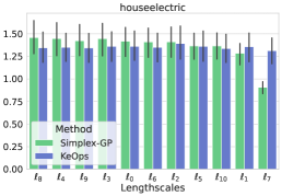
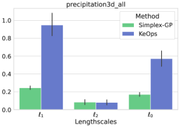
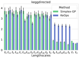
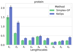
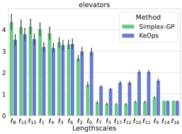
Figure 8: For all our benchmark UCI datasets, when comparing the lengthscales between those learned by Simplex-GPs, and those learned by exact GPs using KeOps, we find that the learned values agree in terms of determined relevance. The label $\ell_{d}$ refers to the lengthscale learned for dimension $d$.

References

- Adams et al. (2009) Adams, A., Gelfand, N., Dolson, J., and Levoy, M. Gaussian kd-trees for fast high-dimensional filtering. In ACM SIGGRAPH 2009 papers. 2009.
- Adams et al. (2010) Adams, A., Baek, J., and Davis, M. A. Fast high‐dimensional filtering using the permutohedral lattice. Computer Graphics Forum, 2010.
- Aurich & Weule (1995) Aurich, V. and Weule, J. Non-linear gaussian filters performing edge preserving diffusion. In DAGM-Symposium, 1995.
- Baek et al. (2012) Baek, J., Adams, A., and Dolson, J. Lattice-based high-dimensional gaussian filtering and the permutohedral lattice. Journal of Mathematical Imaging and Vision, 2012.
- Balandat et al. (2019) Balandat, M., Karrer, B., Jiang, D. R., Daulton, S., Letham, B., Wilson, A., and Bakshy, E. Botorch: Programmable bayesian optimization in pytorch. ArXiv, 2019.
- Barron & Poole (2016) Barron, J. T. and Poole, B. The fast bilateral solver. In European Conference on Computer Vision. Springer, 2016.
- Birchfield (2016) Birchfield, S. Image filtering. In Image Processing and Analysis, chapter 3. 2016.
- Brown et al. (2020) Brown, T. B., Mann, B., Ryder, N., Subbiah, M., Kaplan, J., Dhariwal, P., Neelakantan, A., Shyam, P., Sastry, G., Askell, A., Agarwal, S., Herbert-Voss, A., Krueger, G., Henighan, T., Child, R., Ramesh, A., Ziegler, D. M., Wu, J., Winter, C., Hesse, C., Chen, M., Sigler, E., Litwin, M., Gray, S., Chess, B., Clark, J., Berner, C., McCandlish, S., Radford, A., Sutskever, I., and Amodei, D. Language models are few-shot learners. In Advances in Neural Information Processing Systems 33: Annual Conference on Neural Information Processing Systems 2020, NeurIPS 2020, December 6-12, 2020, virtual, 2020.
- Candela & Rasmussen (2005) Candela, J. Q. and Rasmussen, C. A unifying view of sparse approximate gaussian process regression. J. Mach. Learn. Res., 2005.
- Charlier et al. (2020) Charlier, B., Feydy, J., Glaunès, J. A., Collin, F.-D., and Durif, G. Kernel operations on the GPU, with autodiff, without memory overflows. arXiv preprint arXiv:2004.11127, 2020.
- Chen et al. (2007) Chen, J., Paris, S., and Durand, F. Real-time edge-aware image processing with the bilateral grid. ACM Transactions on Graphics (TOG), (3), 2007.
- Conway & Sloane (1988) Conway, J. H. and Sloane, N. Sphere packings, lattices and groups. In Grundlehren der mathematischen Wissenschaften, 1988.
- Deisenroth et al. (2013) Deisenroth, M., Neumann, G., and Peters, J. A survey on policy search for robotics. Found. Trends Robotics, 2013.
- Deng et al. (2009) Deng, J., Dong, W., Socher, R., Li, L., Li, K., and Li, F. Imagenet: A large-scale hierarchical image database. In 2009 IEEE Computer Society Conference on Computer Vision and Pattern Recognition (CVPR 2009), 20-25 June 2009, Miami, Florida, USA, 2009.
- Dua & Graff (2017) Dua, D. and Graff, C. UCI machine learning repository, 2017.
- Fattal et al. (2007) Fattal, R., Agrawala, M., and Rusinkiewicz, S. Multiscale shape and detail enhancement from multi-light image collections. ACM Trans. Graph., (3), 2007.
- Frazier (2018) Frazier, P. A tutorial on bayesian optimization. ArXiv, 2018.
- Gardner et al. (2018a) Gardner, J. R., Pleiss, G., Weinberger, K. Q., Bindel, D., and Wilson, A. G. Gpytorch: Blackbox matrix-matrix gaussian process inference with GPU acceleration. In Advances in Neural Information Processing Systems 31: Annual Conference on Neural Information Processing Systems 2018, NeurIPS 2018, December 3-8, 2018, Montréal, Canada, 2018a.
- Gardner et al. (2018b) Gardner, J. R., Pleiss, G., Wu, R., Weinberger, K. Q., and Wilson, A. G. Product kernel interpolation for scalable gaussian processes. In International Conference on Artificial Intelligence and Statistics, AISTATS 2018, 9-11 April 2018, Playa Blanca, Lanzarote, Canary Islands, Spain, Proceedings of Machine Learning Research, 2018b.
- Golub & Loan (1996) Golub, G. and Loan, C. Matrix computations (3rd ed.). In Johns Hopkins Press, 1996.
- Greengard & Strain (1991) Greengard, L. and Strain, J. The fast gauss transform. SIAM Journal on Scientific and Statistical Computing, (1), 1991.
- He et al. (2010) He, K., Sun, J., and Tang, X. Guided image filtering. In European conference on computer vision. Springer, 2010.
- Hensman et al. (2013) Hensman, J., Fusi, N., and Lawrence, N. D. Gaussian processes for big data. In Proceedings of the Twenty-Ninth Conference on Uncertainty in Artificial Intelligence, UAI 2013, Bellevue, WA, USA, August 11-15, 2013, 2013.
- Hensman et al. (2015a) Hensman, J., de G. Matthews, A. G., Filippone, M., and Ghahramani, Z. MCMC for variationally sparse gaussian processes. In Advances in Neural Information Processing Systems 28: Annual Conference on Neural Information Processing Systems 2015, December 7-12, 2015, Montreal, Quebec, Canada, 2015a.
- Hensman et al. (2015b) Hensman, J., de G. Matthews, A. G., and Ghahramani, Z. Scalable variational gaussian process classification. In Proceedings of the Eighteenth International Conference on Artificial Intelligence and Statistics, AISTATS 2015, San Diego, California, USA, May 9-12, 2015, JMLR Workshop and Conference Proceedings, 2015b.
- Izmailov et al. (2018) Izmailov, P., Novikov, A., and Kropotov, D. Scalable gaussian processes with billions of inducing inputs via tensor train decomposition. In International Conference on Artificial Intelligence and Statistics, AISTATS 2018, 9-11 April 2018, Playa Blanca, Lanzarote, Canary Islands, Spain, Proceedings of Machine Learning Research, 2018.
- Kiefel et al. (2014) Kiefel, M., Jampani, V., and Gehler, P. V. Permutohedral lattice cnns. arXiv preprint arXiv:1412.6618, 2014.
- Krähenbühl & Koltun (2011) Krähenbühl, P. and Koltun, V. Efficient inference in fully connected crfs with gaussian edge potentials. In Advances in Neural Information Processing Systems 24: 25th Annual Conference on Neural Information Processing Systems 2011. Proceedings of a meeting held 12-14 December 2011, Granada, Spain, 2011.
- Liu et al. (2020) Liu, H., Ong, Y., Shen, X., and Cai, J. When gaussian process meets big data: A review of scalable gps. IEEE Transactions on Neural Networks and Learning Systems, 2020.
- Matthews et al. (2017) Matthews, A., van der Wilk, M., Nickson, T., Fujii, K., Boukouvalas, A., León-Villagrá, P., Ghahramani, Z., and Hensman, J. Gpflow: A gaussian process library using tensorflow. J. Mach. Learn. Res., 2017.
- Paris & Durand (2006) Paris, S. and Durand, F. A fast approximation of the bilateral filter using a signal processing approach. In ECCV, 2006.
- Paszke et al. (2019) Paszke, A., Gross, S., Massa, F., Lerer, A., Bradbury, J., Chanan, G., Killeen, T., Lin, Z., Gimelshein, N., Antiga, L., Desmaison, A., Köpf, A., Yang, E., DeVito, Z., Raison, M., Tejani, A., Chilamkurthy, S., Steiner, B., Fang, L., Bai, J., and Chintala, S. Pytorch: An imperative style, high-performance deep learning library. In Advances in Neural Information Processing Systems 32: Annual Conference on Neural Information Processing Systems 2019, NeurIPS 2019, December 8-14, 2019, Vancouver, BC, Canada, 2019.
- Potapczynski et al. (2021) Potapczynski, A., Wu, L., Biderman, D., Pleiss, G., and Cunningham, J. P. Bias-free scalable gaussian processes via randomized truncations. CoRR, abs/2102.06695, 2021.
- Rasmussen & Williams (2005) Rasmussen, C. E. and Williams, C. K. I. Gaussian Processes for Machine Learning (Adaptive Computation and Machine Learning). 2005.
- Salimbeni & Deisenroth (2017) Salimbeni, H. and Deisenroth, M. P. Doubly stochastic variational inference for deep gaussian processes. In Advances in Neural Information Processing Systems 30: Annual Conference on Neural Information Processing Systems 2017, December 4-9, 2017, Long Beach, CA, USA, 2017.
- Silverman (1985) Silverman, B. Some aspects of the spline smoothing approach to non‐parametric regression curve fitting. Journal of the royal statistical society series b-methodological, 1985.
- Snelson & Ghahramani (2007) Snelson, E. and Ghahramani, Z. Local and global sparse gaussian process approximations. In AISTATS, 2007.
- Su et al. (2018) Su, H., Jampani, V., Sun, D., Maji, S., Kalogerakis, E., Yang, M., and Kautz, J. Splatnet: Sparse lattice networks for point cloud processing. In 2018 IEEE Conference on Computer Vision and Pattern Recognition, CVPR 2018, Salt Lake City, UT, USA, June 18-22, 2018, 2018.
- Titsias (2009) Titsias, M. K. Variational learning of inducing variables in sparse gaussian processes. In AISTATS, 2009.
- Tomasi & Manduchi (1998) Tomasi, C. and Manduchi, R. Bilateral filtering for gray and color images. Sixth International Conference on Computer Vision (IEEE Cat. No.98CH36271), 1998.
- Wang et al. (2019) Wang, K. A., Pleiss, G., Gardner, J. R., Tyree, S., Weinberger, K. Q., and Wilson, A. G. Exact gaussian processes on a million data points. In Advances in Neural Information Processing Systems 32: Annual Conference on Neural Information Processing Systems 2019, NeurIPS 2019, December 8-14, 2019, Vancouver, BC, Canada, 2019.
- Wilson et al. (2015) Wilson, A., Dann, C., and Nickisch, H. Thoughts on massively scalable gaussian processes. ArXiv, 2015.
- Wilson & Nickisch (2015) Wilson, A. G. and Nickisch, H. Kernel interpolation for scalable structured gaussian processes (KISS-GP). In Proceedings of the 32nd International Conference on Machine Learning, ICML 2015, Lille, France, 6-11 July 2015, JMLR Workshop and Conference Proceedings, 2015.
- Zhu et al. (2015) Zhu, Q., Mai, J., and Shao, L. A fast single image haze removal algorithm using color attenuation prior. IEEE transactions on image processing, (11), 2015.