Doubly Non-Central Beta Matrix Factorization for DNA Methylation Data

Abstract

We present a new non-negative matrix factorization model for $(0,1)$ bounded-support data based on the doubly non-central beta (DNCB) distribution, a generalization of the beta distribution. The expressiveness of the DNCB distribution is particularly useful for modeling DNA methylation datasets, which are typically highly dispersed and multi-modal; however, the model structure is sufficiently general that it can be adapted to many other domains where latent representations of $(0,1)$ bounded-support data are of interest. Although the DNCB distribution lacks a closed-form conjugate prior, several augmentations let us derive an efficient posterior inference algorithm composed entirely of analytic updates. Our model improves out-of-sample predictive performance on both real and synthetic DNA methylation datasets over state-of-the-art methods in bioinformatics. In addition, our model yields meaningful latent representations that accord with existing biological knowledge.

1 Introduction

DNA methylation is a mechanism by which epigenetic changes to DNA can modify the transcription of nearby genes. These epigenetic changes can activate oncogenes or inactivate tumor suppressors to drive the onset of cancer and other diseases [Laird, 2010]. Discovering novel subtypes of cancer that share underlying patterns of DNA methylation is of interest to scientists, who seek to better understand the role of DNA methylation in cancer development, and to clinicians, who seek to refine existing cancer treatment strategies. To achieve this goal, computational biologists routinely apply dimensionality reduction methods to DNA methylation datasets in order to discover latent representations that are both scientifically interesting and clinically useful.

A DNA methylation dataset typically consists of an $N\times M$ sample-by-gene matrix of bounded-support data $\mathcal{B}\in(0,1)^{N\times M}$, where the number of samples $N$ is often far exceeded by the number of genes $M$. A single element of this matrix $\beta_{ij}\in(0,1)$ represents the degree of methylation for regions of the genome near gene $j$ in sample $i$.

The most commonly used dimensionality reduction methods are principal component analysis (PCA) [Teschendorff et al., 2007] and non-negative matrix factorization (NMF) [Zhuang et al., 2012]. These methods are based on Gaussian assumptions that are inappropriate for $(0,1)$ bounded-support data. As a result, they fit DNA methylation datasets worse than methods that are based on more appropriate probabilistic assumptions [Ma et al., 2014].

The few existing non-Gaussian dimensionality reduction methods for DNA methylation datasets almost all assume that the elements of a sample-by-gene matrix are beta-distributed. Indeed, this assumption is so standard in bioinformatics that the elements are typically referred to as “beta values” [Kuan et al., 2010]. Of these existing methods, the most expressive is beta-gamma non-negative matrix factorization (BG-NMF), a non-negative matrix factorization model with a beta likelihood [Ma et al., 2014].

Although the beta distribution is a natural choice for modeling data with bounded support between 0 and 1, it is a challenging distribution with which to build probabilistic models due its lack of a closed-form conjugate prior [Fink, 1997]. In general, there are few tractable and modular motifs for deriving posterior inference algorithms for models that assume a beta likelihood. Models that do not make overly simplistic assumptions tend to be accompanied by posterior inference algorithms that are highly tailored to their specific structures, making them difficult to modify or extend. Moreover, these inference algorithms typically rely on approximations that hamper precise quantification of uncertainty, which is of particular interest in biomedical settings where datasets are often small and properly calibrated decisions are critical.

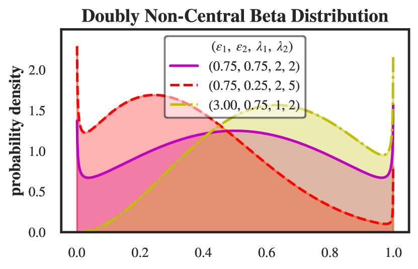
Figure 1: The DNCB distribution can take multi-modal shapes when $\epsilon_{1}<1$ or $\epsilon_{2}<1$. This expressiveness is particularly useful when modeling DNA methylation datasets, which are typically highly dispersed and multi-modal. The DNCB distribution can also look like the standard beta (see fig. 8 of the appendix).

In this paper, we therefore introduce a new non-negative matrix factorization model for $(0,1)$ bounded-support data based on the doubly non-central beta (DNCB) distribution [Ongaro and Orsi, 2015]. The DNCB distribution is a four-parameter generalization of the beta distribution that can take a more flexible set of shapes over the $(0,1)$ interval, including those that are multi-modal (see fig. 1). Although our model was developed specifically for DNA methylation datasets, the model structure is sufficiently general that it can be adapted to many other domains where latent representations of $(0,1)$ bounded-support data are of interest.

The property of the DNCB distribution that makes it particularly useful for building probabilistic models is that it can be augmented in terms of a pair of Poisson-distributed auxiliary variables. With this augmentation, we can build tractable dimensionality reduction methods for $(0,1)$ bounded-support data based on Poisson factorization models, which are well studied and easy to build on [Titsias, 2007, Cemgil, 2009, Zhou et al., 2012, Gopalan et al., 2012, Paisley et al., 2015].

We develop an accompanying Gibbs sampler by appealing to special relationships between the beta, gamma, and Poisson distributions to obtain analytic updates that involve the Bessel distribution [Yuan and Kalbfleisch, 2000]. Our Gibbs sampler is asymptotically guaranteed to sample from the exact posterior distribution and it is general to any Poisson factorization model for which analytic updates already exist.

We compare our model’s out-of-sample predictive performance to that of state-of-the-art methods in bioinformatics. We find that our model performs significantly better than NMF, which assumes a Gaussian likelihood, and BG-NMF, which assumes a beta likelihood, for real DNA methylation datasets. We also use a biologically motivated synthetic data generator [de Souza et al., 2020] to create synthetic datasets that enable us to study our model’s suitability for $(0,1)$ bounded-support data that may arise in other domains.

Finally, we explore our model’s ability to discover meaningful latent representations by applying our model to a microarray dataset composed of samples from six different cancer types. We demonstrate that the resulting representations accord with existing epigenetic knowledge about the gene pathways that play major roles in the six different cancer types.

Contributions and roadmap.

To summarize, in this paper, we make three main contributions, outlined below:

1. A new non-negative matrix factorization model for data with bounded support between 0 and 1 based on the doubly non-central beta (DNCB) distribution (section 2).

2. An auxiliary variable scheme, involving several augmentations, that lets us develop an efficient Gibbs sampler composed entirely of analytic updates (section 4).

3. A study of our model’s out-of-sample predictive performance on real and synthetic DNA methylation datasets (section 5), and a case study demonstrating that the model also yields meaningful latent representations that accord with existing biological knowledge (section 6).

2 DNCB matrix factorization

Here, we present doubly non-central beta matrix factorization (DNCB-MF), a new model that assumes each element $\beta_{ij}\in(0,1)$ in a sample-by-gene matrix is drawn as follows:

$$\beta_{ij} \sim\textrm{DNCB}\left(\epsilon_{0}^{{(1)}},\epsilon_{0}^{{(2)}},\lambda_{ij}^{{(1)}},\lambda_{ij}^{{(2)}}\right),$$ (1)

where $\epsilon_{0}^{{(1)}}$ and $\epsilon_{0}^{{(2)}}$ are shared across all $i$ and $j$ and $\lambda_{ij}^{{(1)}}$ and $\lambda_{ij}^{{(2)}}$ are linear functions of low-rank latent factors—i.e.,

$$\lambda_{ij}^{{(1)}}=\sum_{k=1}^{K}\theta_{ik}^{{(1)}}\phi_{kj} \;\;\;\;\textrm{and}\;\;\;\;\lambda_{ij}^{{(2)}}=\sum_{k=1}^{K}\theta_{ik}^{{(2)}}\phi_{kj}.$$ (2)

DNCB-MF is one instance of a class of models for $(0,1)$ bounded-support data that factorize the “non-centrality” parameters of the DNCB distribution, as defined below.

Definition 1.

The doubly non-central beta (DNCB) distribution is continuous over the support $\beta\in(0,1)$ and defined by “shape” parameters $\epsilon_{1},\epsilon_{2}>0$, “non-centrality” parameters $\lambda_{1},\lambda_{2}\geq 0$, and the following probability density function:

$$\textrm{DNCB}\,(\beta\,;\,\epsilon_{1},\epsilon_{2},\lambda_{1},\lambda_{2})$$

$$\hskip 6.00006pt=\text{Beta}\left(\beta;\,\epsilon_{1},\epsilon_{2}\right)\,e^{-\lambda_{\bullet}}\,\Psi_{2}\big{[}\epsilon_{\bullet};\epsilon_{1},\epsilon_{2};\,\lambda_{1}\beta,\,\lambda_{2}(1\!-\!\beta)\big{]},$$

where $\lambda_{\bullet}=\lambda_{1}+\lambda_{2}$, $\epsilon_{\bullet}=\epsilon_{1}+\epsilon_{2}$, and $\Psi_{2}[\cdot;\cdot,\cdot;\cdot,\cdot]$ denotes Humbert’s confluent hypergeometric function [Srivastava and Karlsson, 1985, Ongaro and Orsi, 2015].

The key property of the DNCB distribution that makes it particularly useful for building probabilistic models is that it can be augmented in terms of a pair of Poisson-distributed auxiliary variables, as defined below.

Definition 2.

A random variable $\beta\!\sim\!\textrm{DNCB}(\epsilon_{1},\epsilon_{2},\lambda_{1},\lambda_{2})$ can be drawn from a standard beta distribution conditioned on two Poisson-distributed auxiliary variables as follows:

$$y_{1}\sim\textrm{Pois}\left(\lambda_{1}\right) \;\;\;\;\textrm{and}\;\;\;\;y_{2}\sim\textrm{Pois}\left(\lambda_{2}\right),$$ (3)

$$(\beta\,|\,y_{1},y_{2}) \sim\textrm{Beta}\left(\epsilon_{1}\!+\!y_{1},\,\epsilon_{2}\!+\!y_{2}\right).$$ (4)

Under the Poisson-randomized representation in definition 2, we can combine eqs. 1 and 2 to express DNCB-MF as

$$y_{ij}^{{(r)}}\!\sim\!\textrm{Pois}\Big{(}\sum_{k=1}^{K}\theta_{ik}^{{(r)}}\phi_{kj}\Big{)}\;\textrm{ for }r\in\{1,2\},$$ (5)

$$\beta_{ij}\sim\textrm{Beta}\left(\epsilon_{0}^{{(1)}}\!+\!y_{ij}^{{(1)}},\,\epsilon_{0}^{{(2)}}\!+\!y_{ij}^{{(2)}}\right),$$ (6)

which connects Poisson factorization to a beta likelihood.

To complete the model, we place gamma priors over the factors, as is standard for Poisson factorization models:

$$\theta_{ik}^{{(1)}},\theta_{ik}^{{(2)}} \sim\textrm{Gam}(a_{0},b_{0}),$$ (7)

$$\phi_{kj} \sim\textrm{Gam}(e_{0},f_{0}).$$ (8)

Interpretation of the auxiliary counts.

Intuitively, the Poisson-distributed auxiliary variables $y_{ij}^{{(1)}}$ and $y_{ij}^{{(2)}}$ perturb the conditional distribution of $\beta_{ij}$ away from a shared background distribution, $\textrm{Beta}\big{(}\epsilon_{0}^{{(1)}},\epsilon_{0}^{{(2)}}\big{)}$. If $y_{ij}^{{(1)}}>y_{ij}^{{(2)}}$, the distribution shifts toward values closer to 0; conversely, if $y_{ij}^{{(2)}}>y_{ij}^{{(1)}}$, the distribution shifts toward 1. Moreover, as the overall magnitude of $y_{ij}^{{(\bullet)}}=y_{ij}^{{(1)}}\!+\!y_{ij}^{{(2)}}$ increases, the distribution concentrates around its mean which equals

$$\mathbb{E}[\beta_{ij}\,|\,y_{ij}^{{(1)}},y_{ij}^{{(2)}}]=\tfrac{\epsilon_{0}^{{(1)}}+y_{ij}^{{(1)}}}{\epsilon_{0}^{{(\bullet)}}+y_{ij}^{{(\bullet)}}}.$$ (9)

The effect of the non-centrality parameters (i.e., the means of the Poisson-distributed auxiliary variables) on the DNCB marginal distribution of $\beta_{ij}$ can be explained similarly. Because $\mathbb{E}[y_{ij}^{{(r)}}]=\lambda_{ij}^{{(r)}}$ for $r\in\{1,2\}$, a large $\lambda_{ij}^{{(1)}}$, relative to $\lambda_{ij}^{{(2)}}$, shifts the density toward 0, while a large $\lambda_{ij}^{{(\bullet)}}=\lambda_{ij}^{{(1)}}+\lambda_{ij}^{{(2)}}$ concentrates the distribution around its mean, whose functional form is in appendix A.

Interpretation of the latent factors.

The latent factor $\phi_{kj}$ represents how relevant gene $j$ is in latent component $k$. The largest elements of the vector $\boldsymbol{\phi}_{k}\in\mathbb{R}_{+}^{M}$ can therefore be interpreted as representing a “pathway” of genes that exhibit correlated patterns of methylation. The latent factors $\theta_{ik}^{{(1)}}$ and $\theta_{ik}^{{(2)}}$ represent how methylated or unmethylated, respectively, the genes in pathway $k$ are in sample $i$. As $\theta_{ik}^{{(1)}}$ increases, relative to $\theta_{ik}^{{(2)}}$, the rate of $y_{ij}^{{(1)}}$ increases, relative to the rate of $y_{ij}^{{(2)}}$, and the distribution of $\beta_{ij}$ shifts toward 0. A convenient way to jointly summarize $\theta_{ik}^{{(1)}}$ and $\theta_{ik}^{{(2)}}$ is

$$\rho_{ik}=\frac{\theta_{ik}^{{(1)}}}{\theta_{ik}^{{(1)}}+\theta_{ik}^{{(2)}}},$$ (10)

where $\rho_{ik}\gg 0.5$ means pathway $k$ is hypermethylated in sample $i$ and $\rho_{ik}\ll 0.5$ means pathway $k$ is hypomethylated in sample $i$. The vector $\boldsymbol{\rho}_{i}\in(0,1)^{K}$ can also be interpreted as an embedding of sample $i$. We show these embeddings can be used to guide exploratory analyses in section 5.

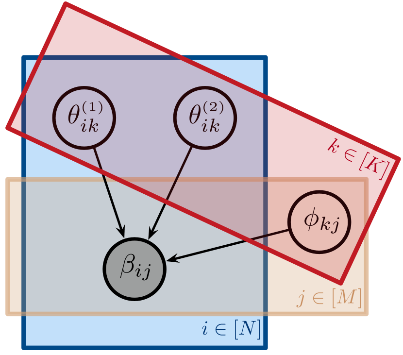
(a) The graphical model for BG-NMF [Ma et al., 2015] and for the form of DNCB-MF given in eq. 1, where all of the auxiliary variables have been marginalized out. 

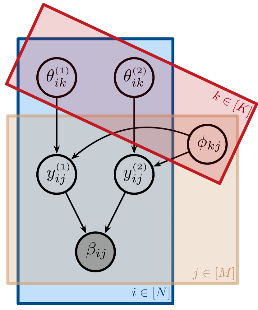
(b) The Poisson-randomized beta form of DNCB-MF given in eqs. 5 and 6. The data’s dependence on the factors flows through the auxiliary variables $y_{ij}^{{(1)}}$ and $y_{ij}^{{(2)}}$. 

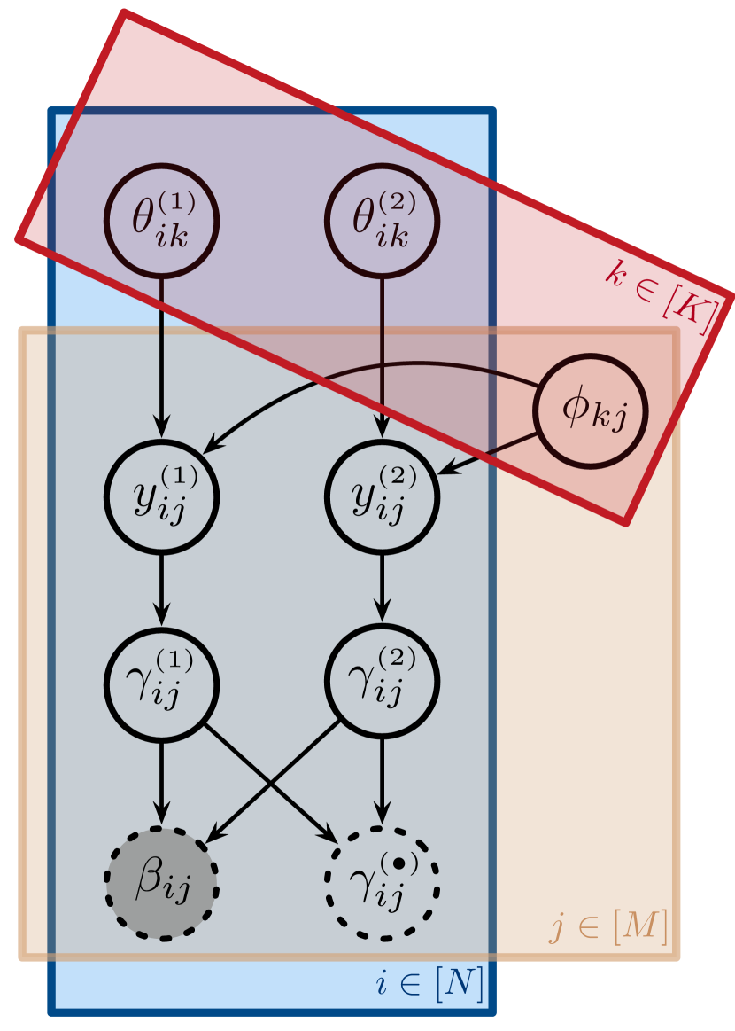
(c) The fully augmented form of DNCB-MF given in eqs. 14 and 15, where $\beta_{ij}$ is determined by $\gamma_{ij}^{{(1)}}$ and $\gamma_{ij}^{{(2)}}$. This form is particularly useful for posterior inference. 

Figure 2: A graphical comparison of related generative processes. All hyperparameters (including $\epsilon_{0}^{{(1)}}$ and $\epsilon_{0}^{{(2)}}$ for DNCB-MF) are omitted for ease of comparison. The plate notation represents exchangeability across the specified indices. Shaded nodes are observed variables; unshaded nodes are latent variables. Solid edges denote random variables; dotted edges denote deterministic variables. 

3 Related work

In this section, we briefly review the most closely related dimensionality reduction methods, with an emphasis on the methods that are commonly used for DNA methylation datasets. We draw connections to our model as appropriate.

PCA and NMF. Non-negative matrix factorization (NMF) [Lee and Seung, 1999] factorizes an $N\times M$ matrix into two non-negative latent factor matrices $\Theta\in\mathbbm{R}_{+}^{N\times K}$ and $\Phi\in\mathbbm{R}_{+}^{K\times M}$. This is typically achieved by minimizing the Frobenius norm of the reconstruction error subject to a non-negativity constraint on the latent factor matrices as:

$$\Theta^{*},\Phi^{*}\in\underset{\Theta,\Phi}{\textrm{argmin}}\,\lVert\mathcal{B}-\Theta\Phi\rVert_{\textrm{F}}\;\;\textrm{ s.t. }\;\;\Theta,\Phi\geq 0.$$ (11)

When fit using this Frobenius loss, NMF can be viewed as performing maximum likelihood estimation (MLE) in a Gaussian model that is truncated so that $\beta_{ij}\in\mathbbm{R}_{+}$:

$$\beta_{ij}\sim\textrm{TruncNorm}(\sum_{k=1}^{K}\theta_{ik}\phi_{kj},\,\sigma_{0}).$$ (12)

Principal component analysis (PCA) involves a similar optimization but without the non-negativity constraint on the latent factor matrices. PCA can be viewed as performing MLE in a standard (i.e., non-truncated) Gaussian model.

Both PCA and NMF are commonly used in bioinformatics and have been used for DNA methylation datasets, where NMF perform betters due to its non-negativity constraint [Teschendorff et al., 2007, Zhuang et al., 2012]. In addition, NMF is often preferred because of the “parts-based” interpretation of its non-negative latent factors.

Non-Gaussian mixture models. Several non-Gaussian clustering methods and mixture models have been developed specifically for DNA methylation datasets; see Ma et al. [2014] for a survey. Some of these models, like the recursive-partitioning beta mixture model of Houseman et al. [2008], assume a beta likelihood. Although these models make probabilistic assumptions that are appropriate for $(0,1)$ bounded-support data, they yield less expressive latent representations than admixture models such as NMF.

BG-NMF. Our model is most closely related to beta-gamma non-negative matrix factorization (BG-NMF), which was developed by Ma et al. [2015] specifically for DNA methylation datasets. BG-NMF is the first (and, to our knowledge, only) matrix factorization model to assume a beta likelihood. Specifically, it assumes that each element $\beta_{ij}\in(0,1)$ in a sample-by-gene matrix is drawn as follows:

$$\beta_{ij} \sim\textrm{Beta}\left(\alpha_{ij}^{{(1)}},\alpha_{ij}^{{(2)}}\right),$$ (13)

where the two “shape” parameters $\alpha_{ij}^{{(1)}}$ and $\alpha_{ij}^{{(2)}}$ are defined to be the same linear functions of low-rank latent factors as those given in eq. 2. BG-NMF also places the same gamma priors over these factors as those given in eqs. 7 and 8.

We provide a graphical comparison of BG-NMF and DNCB-MF in fig. 2. DNCB-MF and BG-NMF both factorize a sample-by-gene matrix into three non-negative latent factor matrices; however, DNCB-MF factorizes the non-centrality parameters of the DNCB distribution, while BG-NMF factorizes the shape parameters of the beta distribution.

Deriving an efficient and modular posterior inference algorithm for BG-NMF is hampered by the lack of a closed-form conjugate prior for the beta distribution. Ma et al. [2015] propose a variational inference algorithm that maximizes nested lower bounds on the model evidence. Their derivation is sophisticated, but highly tailored to the specific structure of the model, which makes the model difficult to modify or extend. Moreover, the quality of this algorithm’s approximation to the posterior distribution is not well understood. For biomedical settings, in which precise quantification of uncertainty is often necessary, the lack of an efficient MCMC algorithm therefore limits BG-NMF’s applicability.

4 Posterior Inference

Given an $N\times M$ sample-by-gene matrix of bounded-support data $\mathcal{B}\in(0,1)^{N\times M}$, the goal is to approximate the posterior distribution over the latent factor matrices $P(\Theta^{{(1)}},\Theta^{{(2)}},\Phi\,|\,\mathcal{B})$. Like the beta distribution, the DNCB distribution lacks a closed-form conjugate prior; however, it admits several augmentations that let us exploit special relationships between the beta, gamma, and Poisson distributions to derive an auxiliary-variable Gibbs sampler whose stationary distribution is the exact posterior. Moreover, this Gibbs sampler is composed entirely of closed-form complete conditionals that can be sampled from efficiently.

Below, we introduce auxiliary variables that augment DNCB-MF to create conditionally conjugate links to the latent factors. Specifically, we work within the Poisson-randomized beta form of the model given in eqs. 5 and 6, which links $\beta_{ij}$ to a pair of Poisson-distributed auxiliary variables $y_{ij}^{{(r)}}\sim\textrm{Pois}(\lambda_{ij}^{{(r)}})$ for $r\in\{1,2\}$, whose rates $\lambda_{ij}^{{(r)}}$ are factorized into the latent factors. Conditioned on these auxiliary variables, the updates for the latent factors follow from gamma–Poisson matrix factorization [Cemgil, 2009].

In light of this, the only thing that is needed is to derive an efficient Gibbs sampler is a way to sample the Poisson-distributed auxiliary variables from their complete conditionals. Our approach relies on further augmenting the conditional likelihood using the following definition.

Definition 3.

A beta random variable $\beta\!\sim\!\textrm{Beta}(\alpha_{1},\alpha_{2})$ can be simulated as $\beta\!=\!\tfrac{\gamma_{1}}{\gamma_{1}\!+\!\gamma_{2}}$, where $\gamma_{r}\!\sim\!\textrm{Gam}\left(\alpha_{r},c\right)$ for $r\in\{1,2\}$ are independent gamma variables with rate $c\!>\!0$.

We can represent the conditional likelihood in eq. 6 as

$$\gamma_{ij}^{{(r)}} \sim\textrm{Gam}\left(\epsilon_{0}^{{(r)}}\!+\!y_{ij}^{{(r)}},1\right)\;\;\text{ for }r\in\{1,2\},$$ (14)

$$\gamma_{ij}^{{(\bullet)}}=\gamma_{ij}^{{(1)}}+\gamma_{ij}^{{(2)}}\;\;\;\textrm{and}\;\;\;\beta_{ij}=\frac{\gamma_{ij}^{{(1)}}}{\gamma_{ij}^{{(\bullet)}}},$$ (15)

which corresponds to the fully augmented form of DNCB-MF shown in fig. 2(c). This form of our model is particularly useful for posterior inference. Indeed, our Gibbs sampler iterates between sampling $y_{ij}^{{(r)}}$ given $\gamma_{ij}^{{(r)}}$ and vice versa.

Sampling $\gamma_{ij}^{{(1)}}$ and $\gamma_{ij}^{{(2)}}$

Because the gamma-distributed auxiliary variables have a deterministic relationship with $\beta_{ij}$, we can sample them from their complete conditional by first sampling their sum $\gamma_{ij}^{{(\bullet)}}$ from its complete conditional and then calculating

$$\gamma_{ij}^{{(1)}}=\beta\gamma_{ij}^{{(\bullet)}}\;\;\;\textrm{and}\;\;\;\gamma_{ij}^{{(2)}}=(1-\beta)\gamma_{ij}^{{(\bullet)}}.$$ (16)

To derive the complete conditional of $\gamma_{ij}^{{(\bullet)}}$, we appeal to the following unique property of gamma-distributed variables.

Definition 4.

For any pair of independent positive random variables $X_{1}$ and $X_{2}$, their sum $X_{\bullet}\!=\!X_{1}+X_{2}$ and their proportion $\tilde{X}\!=\!X_{1}\,/\,(X_{1}+X_{2})$ are marginally independent—that is, $P(X_{\bullet},\tilde{X})\!=\!P(X_{\bullet})\,P(\tilde{X})$—if and only if $X_{1}$ and $X_{2}$ are both gamma-distributed [Lukacs, 1955].

The complete conditional of $\gamma_{ij}^{{(\bullet)}}$ is therefore independent of $\beta_{ij}$ and equal to its distribution under the prior. Because $\gamma_{ij}^{{(\bullet)}}$ is defined as the sum of two gamma-distributed random variables, its complete conditional (and prior) is as follows:

$$\gamma_{ij}^{{(\bullet)}}\sim\textrm{Gam}\left(\epsilon_{0}^{{(\bullet)}}+y_{ij}^{{(\bullet)}},1\right).$$ (17)

Collectively, eqs. 17 and 16 provide an efficient way to sample $\gamma_{ij}^{{(1)}}$ and $\gamma_{ij}^{{(2)}}$ from their complete conditional.

Sampling $y_{ij}^{{(1)}}$ and $y_{ij}^{{(2)}}$

Conditioning on $\gamma_{ij}^{{(1)}}$ and $\gamma_{ij}^{{(2)}}$ renders the Poisson-distributed auxiliary variables $y_{ij}^{{(1)}}$ and $y_{ij}^{{(2)}}$ independent under their complete conditional. Moreover, as shown by the following proposition, their complete conditionals have a closed form.

Definition 5.

If $\gamma\sim\textrm{Gam}(\epsilon\!+\!y,c)$ and $y\sim\textrm{Pois}\left(\lambda\right)$, then the posterior of $y$ is Bessel [Yuan and Kalbfleisch, 2000]:

$$P(y\,|\,\gamma,\epsilon,c,\lambda)=\textrm{Bess}\left(y;\epsilon\!-\!1,\,2\sqrt{c\gamma\lambda}\right),$$ (18)

where the Bessel distribution is defined as

$$\textrm{Bess}\left(y;v,a\right)=\frac{(\tfrac{a}{2})^{2y+v}}{y!\,\Gamma(y+v+1)\,I_{v}(a)}$$ (19)

and where $I_{v}(a)$ is the first type modified Bessel function.

Using this definition, the complete conditional for $y_{ij}^{{(r)}}$ is

$$(y_{ij}^{{(r)}}|-)\sim\textrm{Bess}\left(\epsilon_{0}^{{(r)}}\!-\!1,\,2\sqrt{\gamma_{ij}^{{(r)}}\lambda_{ij}^{{(r)}}}\right).$$ (20)

Devroye [2002] gives methods for efficiently sampling from the Bessel distribution. Although it is still relatively unknown, the Bessel distribution has gained attention in a few recent papers [Zhou et al., 2015, Schein et al., 2019b, a].

Sampling $\theta_{ik}^{{(1)}},\theta_{ik}^{{(2)}},\phi_{kj}$

Conditioned on $y_{ij}^{{(1)}}$ and $y_{ij}^{{(2)}}$, the updates for the latent factors $\theta_{ik}^{{(1)}},\theta_{ik}^{{(2)}},\phi_{kj}$ follow from gamma–Poisson matrix factorization. We provide these updates in appendix B, along with a complete summary of our entire Gibbs sampler.

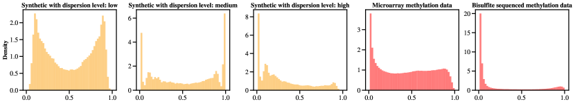
Figure 3: Histograms of the synthetic (yellow) and real (red) datasets. The synthetic datasets were created using Epiclomal with three levels of dispersion. As dispersion increases, values are pushed to the extremes. The high-dispersion data (middle) is most similar to the real data. 

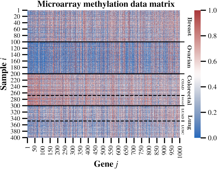
Figure 4: Heatmap of the microarray dataset. Only the first 1,000 (of $M\!=\!$ 5,000) genes are shown. Bright red values are well above 0.5 and indicate that a gene is methylated; blue indicates that a gene is unmethylated. The four (known) cancer types (100 samples from each) are annotated; they clearly display differentiated methylation. 

5 Out-of-Sample Prediction

In this section, we present a study of our model’s out-of-sample predictive performance on both real and synthetic DNA methylation datasets. We compare our model’s performance to that of state-of-the-art models in bioinformatics.

5.1 Datasets

Microarray data.

We used the Cancer Genome Atlas (TCGA) [Tomczak et al., 2015] to compile a dataset of 400 cancer samples whose methylation level at about 27,000 genes was profiled using Illumina 450K BeadChip microarrays. We selected the samples so that there were 100 samples each from four etiologically distinct cancer types: breast, ovarian, colorectal, and lung cancer. The colorectal and lung cancer samples further divide into two subtypes. Although the goal of dimensionality reduction is usually to discover novel subtypes, checking a model’s ability to discover known subtypes can be a way to assess its utility. Microarray data comes processed into “beta values” [Kuan et al., 2010]; we did not process the data any further. Following Ma et al. [2014], we selected the 5,000 genes with the highest variance across the samples to obtain a $400\times 5,000$ sample-by-gene matrix. A heatmap of this matrix is shown in fig. 4.

Bisulfite sequenced methylation data.

We downloaded the dataset studied by Sheffield et al. [2017]. This dataset consists of 156 Ewing sarcoma cancer samples and 32 healthy samples ($N\!=\!188$), whose methylation was profiled using bisulfite sequencing (bi-seq). Bi-seq data consists of binary “reads” of methylation at many loci per gene. We processed this data into “beta values” by first counting all the methylated-mapped reads $d_{ij}$ and non-methylated reads $u_{ij}$ for all loci within a given gene $j$ and then calculating $\beta_{ij}=\frac{s_{0}+d_{ij}}{2s_{0}+d_{ij}+u_{ij}}$ with the smoothing term set to $s_{0}\!=\!0.1$. As with the microarray data, we selected the 5,000 genes with the highest variance to obtain a $188\times 5,000$ matrix.

Synthetic data. To study our model’s suitability for $(0,1)$ bounded-support data that may arise in other domains, we created synthetic datasets using the Epiclomal synthetic data generator [de Souza et al., 2020]. Epiclomal simulates single-cell methylation data. To create “bulk” data, similar to the microarray or bi-seq data, we generated and aggregated 100 cells for every sample $i$ for $N=100$ samples at $M=500$ genes. We varied the Epiclomal parameters to generate datasets with three different levels of dispersion—low, medium, and high—where increasing dispersion pushes values toward the extremes of 0 and 1. For each level of dispersion, we generated three datasets, all with the “true” number of components set to $K^{\star}\!=\!10$. We provide a comparison of the synthetic and real datasets’ histograms in fig. 3.

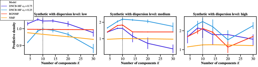
Figure 5: Out-of-sample predictive performance for the synthetic datasets. We generated datasets with three levels of dispersion—low (left), medium (middle), and high (right)—where increasing dispersion pushes values to the extremes of 0 and 1. For each level of dispersion, we generated three datasets; for each dataset, we created three train–test splits by generating three binary masks. For all models with all values of $K$, we used three different random initializations for each dataset and mask combination. For each value of $K$, we plot $\textrm{PPD}^{\frac{1}{|\mathcal{M}|}}$, where $|\mathcal{M}|$ is the number of held-out values, averaged across the initialization, dataset, and mask combinations; error bars indicate 95% confidence intervals. For all three levels of dispersion, most models’ performance peaks at the true number of components $K\!=\!K^{\star}\!=\!10$. NMF always performs worse than BG-NMF; BG-NMF is almost always “sandwiched” between DNCB-MF with $\epsilon_{0}\!=\!0.25$ and DNCB-MF with $\epsilon_{0}\!=\!0.75$ (or vice versa). For the low-dispersion datasets, DNCB-MF with $\epsilon_{0}\!=\!0.75$ performs the best, while DNCB-MF with $\epsilon_{0}\!=\!0.25$ performs worse than than BG-NMF. For the medium- and high-dispersion datasets, DNCB-MF with $\epsilon_{0}=0.25$ performs the best. Intuitively, this makes sense: as the DNCB shape parameters get smaller, the density concentrates at the extremes (see fig. 1). 

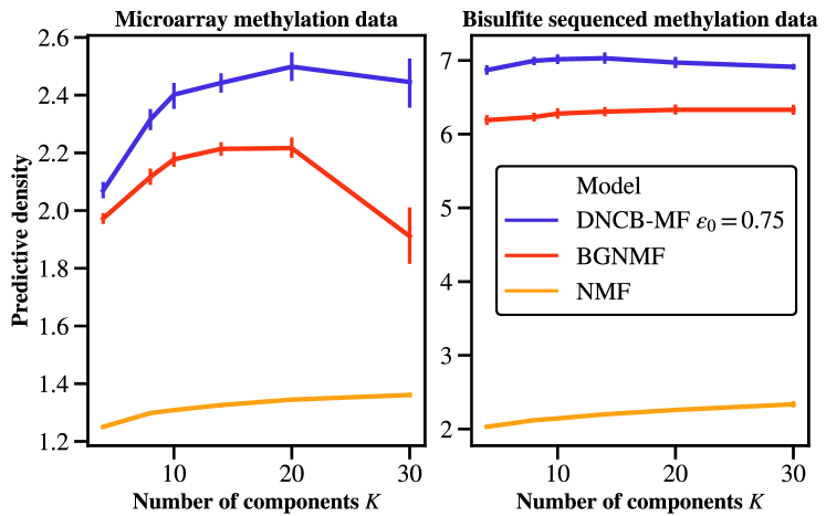
Figure 6: Out-of-sample predictive performance for the two real datasets described in section 5.1. For both, DNCB-MF with $\epsilon_{0}\!=\!0.75$ performs significantly better than NMF and BG-NMF.

5.2 Models

We compare our model’s out-of-sample predictive performance to that of BG-NMF and NMF. BG-NMF is a is a state-of-the-art matrix factorization model for DNA methylation data that differs from DNCB-MF by assuming a beta likelihood instead of a DNCB likelihood; NMF serves as a simple baseline because it is so commonly used.

Setting $K$.

For all models in all experiments, we used $K\in\{4,8,10,14,20,30\}$. These values are centered around $K\!=\!14$, which Ma et al. [2014] report as being optimal for BG-NMF when modeling DNA methylation datasets that are similar in composition to our microarray dataset.

DNCB-MF.

We implemented the Gibbs sampler described in section 4 in Cython. For all experiments, we let the Gibbs sampler “burn in” for 1,000 iterations and then ran it for another 2,000 iterations, saving every $20^{\textrm{th}}$ sample. We set the hyperparameters for the gamma priors to $a_{0}\!=\!b_{0}\!=\!e_{0}\!=\!f_{0}\!=\!0.1$ and set the two DNCB shape parameters to $\epsilon_{0}^{{(1)}}\!=\!\epsilon_{0}^{{(2)}}\!=\!\epsilon_{0}\!=\!0.75$. For the synthetic datasets, we also experimented with setting the shape parameters to $\epsilon_{0}\!=\!0.25$.

BG-NMF.

We implemented BG-NMF in Python and set the hyperparameters for the gamma priors to the values described above for DNCB-MF. We set all other hyperparameters to the values recommended by Ma et al. [2014].

NMF.

We used the implementation of NMF in Scikit-learn [Pedregosa et al., 2011] with the default settings.

Code.

We have released our implementations of DNCB-MF and BG-NMF. Our code includes fast samplers for the Bessel distribution and an algorithm for computing the density of the DNCB distribution. We have also released the real and synthetic datasets that we used for our experiments.

5.3 Study design

Random masks.

We created three train–test splits for each dataset (real or synthetic) by generating three binary masks $\mathcal{M}$ that “hold out” a random 10% of the sample-by-gene matrix. For all models with all values of $K$, we used three different random initializations for each dataset and mask combination. All models took the mask as input and imputed the held-out values during inference.

Evaluation metric.

To assess out-of-sample predictive performance, we used the pointwise predictive density (PPD) [Gelman et al., 2014]. For NMF, this is as follows:

$$\textrm{PPD}_{\textrm{point}}=\prod_{i,j\in\mathcal{M}}P\big{(}\beta_{ij}\,|\,\Theta^{*},\Phi^{*}\big{)},$$ (21)

where $\Theta^{*}$ and $\Phi^{*}$ are point estimates of NMF’s latent factor matrices and $P(\cdot\,|\,\cdot)$ denotes a Gaussian truncated to $(0,\infty)$.

For BG-NMF and DNCB-MF, the PPD is given by

$$\textrm{PPD}_{\textrm{post}}=\prod_{i,j\in\mathcal{M}}\Big{[}\tfrac{1}{S}\sum_{s=1}^{S}P\big{(}\beta_{ij}\,|\,\Theta^{(1)}_{s},\Theta^{(2)}_{s},\Phi_{s}\big{)}\Big{]},$$ (22)

where $\Theta^{(1)}_{s},\Theta^{(2)}_{s},\Phi_{s}$ are samples from the posterior distribution, either saved during MCMC for DNCB-MF or drawn from the fitted variational distribution for BG-NMF. For both models, we used $S\!=\!100$. The predictive density $P(\cdot|\cdot)$ is the beta distribution for BG-NMF and the DNCB distribution for our model. Computing the DNCB density requires computing Humbert’s confluent hypergeometric function, for which we implemented the algorithm of Orsi [2017].

For all models, we ultimately report $\textrm{PPD}^{\frac{1}{|\mathcal{M}|}}$, where $|\mathcal{M}|$ is the number of held-out values, which is equivalent to the geometric mean of the predictive densities across the held-out values and is therefore comparable across all experiments. We note that this scaled version of PPD is the inverse of perplexity, an evaluation metric that is commonly used to evaluate statistical topic models and language models.

5.4 Results

Out-of-sample predictive performance for the synthetic and real datasets are shown in figs. 5 and 6, respectively. Our model performs significantly better than NMF and BG-NMF. The results for the synthetic datasets reveal an intuitive relationship between the level of dispersion and the two DNCB shape parameters $\epsilon_{0}^{(1)}=\epsilon_{0}^{(2)}=\epsilon_{0}$, with a smaller parameter value yielding better performance for the more highly dispersed datasets. For these datasets, DNCB-MF with $\epsilon_{0}=0.25$ improves performance over both NMF and BG-NMF.

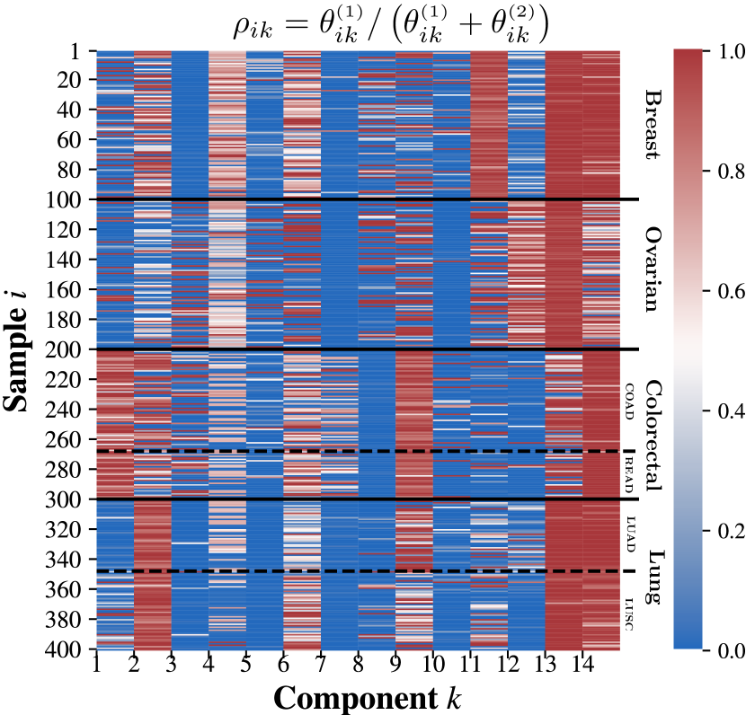
(a) Heatmap of the embedding matrix, as defined in eq. 10.

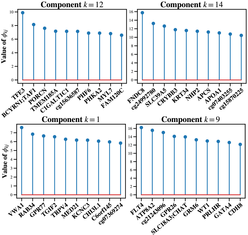
(b) The top ten genes for four components.

Figure 7: The latent representations discovered by DNCB-MF when applied to the microarray dataset. Left: The inferred embedding matrix. The dataset contains four cancer types (separated by horizontal lines); two of these cancer types (colorectal and lung) further divide into two subtypes (separated by horizontal lines). Right: The genes with the ten highest $\phi_{kj}$ values for four components $k=1,9,12,14$.

6 Case study

Here, we explore our model’s ability to discover meaningful latent representations by applying our model to the microarray dataset described in section 5.1 and exploring the resulting representations. The microarray dataset contains samples from four different cancer types: breast, ovarian, colorectal, and lung cancer; the colorectal and lung cancer samples further divide into two subtypes (see fig. 4). We find that the latent representations discovered by our model accord with existing epigenetic knowledge about the gene pathways that play major roles in the six different cancer types.

Figure 7(a) contains the inferred embedding matrix, where each row $\boldsymbol{\rho}_{i}$ is an embedding of sample $i$, as defined in eq. 10. A red value denotes $\rho_{ik}>0.5$ and indicates that the loci proximal to the genes relevant to component $k$ are hypermethylated in sample $i$ according to the model; conversely, a blue value indicates that the loci are hypomethylated according to the model. In fig. 7(b), we additionally show the genes with the ten highest $\phi_{kj}$ values for four components.

Component $k\!=\!1$ has red (high) values for the colorectal cancer samples and blue (low) values for the lung cancer samples, suggesting that the top genes for that component are hypermethylated in colorectal cancer and hypomethylated in lung cancer, respectively. The component stem plot in fig. 7(b) shows that the top genes include RAB34, a member of the Ras oncogene family [Sun et al., 2018]. In general, DNA methylation leads to gene silencing (especially when proximal to the promoter region) and therefore hypomethylation can activate oncogenes like RAB34 [Moore et al., 2013].

The colorectal cancer samples exhibit hypermethylation for component $k\!=\!9$, whose top gene is FLT4. Recent work demonstrates that suppressing FLT4 inhibits cancer metastasis [Xiao et al., 2015]; it is a known therapeutic target.

All samples exhibit hypomethylation for component $k\!=\!12$, except for the ovarian cancer samples. The top gene is TFE3, which promotes activation of the transforming growth factor beta (TGF$\beta$) signaling pathway. TFE3 translocation and subsequent activation is a well-known cause of adult renal cell carcinoma [Sukov et al., 2012].

Conversely, all samples exhibit hypomethylation for component $k\!=\!12$, except for the ovarian cancer samples. The top gene is the fibronectin protein FNDC8. Fibronectin promotes cell migration and invasion in ovarian cancer [Yousif, 2014], so this accords with existing biological knowledge.

7 Conclusion

We presented DNCB-MF, a new non-negative factorization model for $(0,1)$ bounded-support data based on the DNCB distribution. The DNCB distribution is an attractive alternative to the beta distribution. As well as being more expressive, the DNCB distribution admits several augmentations that connect DNCB-MF to Poisson factorization models, which are well studied and easy to build on. Although DNCB-MF was developed specifically for DNA methylation data, the model structure is sufficiently general that it can be adapted to other domains. We showed that DNCB-MF improves out-of-sample predictive performance on both real and synthetic DNA methylation datasets over state-of-the-art methods in bioinformatics and that the resulting representations accord with existing epigenetic knowledge.

8 Acknowledgements

This work was supported in part by National Science Foundation Award 1934846. We also thank Mingyuan Zhou and Daniel Sheldon for their work on a precursor to this model.

Appendix A The DNCB distribution

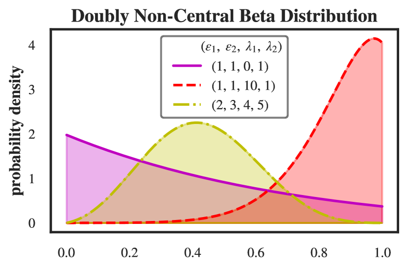
Figure 8: With $\epsilon_{1},\epsilon_{2}\geq 1$, the DNCB distribution takes unimodal shapes over $(0,1)$, similar to the beta distribution; with $\lambda_{1}=\lambda_{2}=0$, the DNCB distribution coincides with the beta distribution.

The DNCB distribution is defined in definition 1. It can take the same set of unimodal shapes over the $(0,1)$ interval as the beta distribution (see fig. 8), as well as multi-modal shapes when the shape parameters $\epsilon_{1},\epsilon_{2}<1$ (see fig. 1).

Ongaro and Orsi [2015] provide a general formula for the moments of the DNCB distribution. Its first moment is

$$\mathbb{E}[\beta]=$$

$$\quad\tfrac{\epsilon_{1}}{\epsilon_{\bullet}e^{\lambda_{\bullet}}}\left[{}_{1}F_{1}\left(\epsilon_{\bullet};\epsilon_{\bullet}\!+\!1;\lambda_{\bullet}\right)+\tfrac{\epsilon_{\bullet}\lambda_{1}}{\epsilon_{1}(\epsilon_{\bullet}\!+\!1)}{}_{1}F_{1}\left(\epsilon_{\bullet}\!+\!1;\epsilon_{\bullet}\!+\!2;\lambda_{\bullet}\right)\right]$$

where ${}_{1}F_{1}(\cdot;\cdot;\cdot)$ denotes Kummer’s confluent hypergeometric function. The second moment is more involved, but also does not involve any special functions beyond ${}_{1}F_{1}(\cdot;\cdot;\cdot)$.

Computing the mean and variance of the DNCB is easy because there are many efficient open-source implementations of ${}_{1}F_{1}(\cdot;\cdot;\cdot)$—e.g., in the Python library scipy [Virtanen et al., 2020]. On the other hand, computing the DNCB density, which we need to assess out-of-sample predictive performance (see section 5), requires computing Humbert’s confluent hypergeometric function $\Psi_{2}[\cdot;\cdot,\cdot;\cdot,\cdot]$ for which we know of no open-source implementations. We therefore implemented the algorithm of Orsi [2017] in Cython. We have released our code for this, along with our implementations of DNCB-MF and BG-NMF and the real and synthetic datasets that we used for our experiments.

Appendix B Posterior Inference

Here, we provide a complete summary of our entire Gibbs sampler. As we described in section 4, the first step is to sample the gamma-distributed auxiliary variables:

$$\big{(}\gamma_{ij}^{{(\bullet)}}\,|\,-\big{)} \sim\textrm{Gam}\left(\epsilon_{0}^{{(\bullet)}}+y_{ij}^{{(\bullet)}},1\right),$$ (23)

$$\gamma_{ij}^{{(1)}}=\beta\gamma_{ij}^{{(\bullet)}} \;\;\;\textrm{and}\;\;\;\gamma_{ij}^{{(2)}}=(1-\beta)\gamma_{ij}^{{(\bullet)}}.$$ (24)

The Poisson-distributed auxiliary variables are then conditionally independent Bessel random variables—i.e.,

$$(y_{ij}^{{(r)}}|-)\sim\textrm{Bess}\left(\epsilon_{0}^{{(r)}}\!-\!1,\,2\sqrt{\gamma_{ij}^{{(r)}}\sum_{k=1}^{K}\theta_{ik}^{{(r)}}\phi_{kj}}\right)$$ (25)

for $r\in\{1,2\}$. Conditioned on these auxiliary counts, the updates for the latent factors follow from gamma–Poisson matrix factorization. First, we represent each count as the sum of $K$ subcounts—i.e., $y_{ij}^{{(r)}}=\sum_{k=1}^{K}y_{ijk}^{{(r)}}$. By Poisson additivity, each of these subcounts is Poisson distributed and their complete conditional is a multinomial distribution:

$$\big{(}\big{(}y_{ijk}^{{(r)}}\big{)}_{k=1}^{K}\,|\,-\big{)}\sim\textrm{Multi}\left(y_{ij}^{{(r)}},\,\left(\tfrac{\theta_{ik}^{{(r)}}\phi_{kj}}{\sum_{k^{\prime}=1}^{K}\theta_{ik^{\prime}}^{{(r)}}\phi_{kj}}\right)_{k=1}^{K}\right).$$ (26)

By Poisson–gamma conjugacy, the complete conditionals of the latent factors, conditioned on the subcounts, are

$$\big{(}\theta_{ik}^{{(r)}}\,|\,-\big{)}\sim\textrm{Gam}\left(a_{0}\!+\!\sum_{j=1}^{M}y_{ijk}^{{(r)}},\,b_{0}\!+\!\sum_{j=1}^{M}\phi_{kj}\right),$$ (27)

$$\big{(}\phi_{kj}\,|\,-\big{)}\sim$$

$$\quad\textrm{Gam}\left(e_{0}\!+\!\sum_{i=1}^{N}\sum_{r=1}^{2}y_{ijk}^{{(r)}},\,f_{0}\!+\!\sum_{i=1}^{N}\sum_{r=1}^{2}\theta_{ik}^{{(r)}}\right).$$ (28)

Equations 23 to B summarize the entire Gibbs sampler for DNCB-MF. Iteratively following these steps is asymptotically guaranteed to sample from the exact posterior.

References

- Cemgil [2009] Ali Taylan Cemgil. Bayesian inference for nonnegative matrix factorisation models. Computational Intelligence and Neuroscience, 2009.
- de Souza et al. [2020] Camila PE de Souza, Mirela Andronescu, Tehmina Masud, Farhia Kabeer, Justina Biele, Emma Laks, Daniel Lai, Patricia Ye, Jazmine Brimhall, Beixi Wang, et al. Epiclomal: Probabilistic clustering of sparse single-cell DNA methylation data. PLoS Computational Biology, 16(9):e1008270, 2020.
- Devroye [2002] Luc Devroye. Simulating Bessel random variables. Statistics & Probability Letters, 57(3):249–257, 2002.
- Fink [1997] Daniel Fink. A compendium of conjugate priors. http://www.stat.columbia.edu/~cook/movabletype/mlm/CONJINTRnew+TEX.pdf, 1997.
- Gelman et al. [2014] Andrew Gelman, Jessica Hwang, and Aki Vehtari. Understanding predictive information criteria for Bayesian models. Statistics and Computing, 24(6):997–1016, 2014.
- Gopalan et al. [2012] Prem K Gopalan, Sean Gerrish, Michael Freedman, David M Blei, and David Mimno. Scalable inference of overlapping communities. Advances in Neural Information Processing Systems, 2012.
- Houseman et al. [2008] E Andres Houseman, Brock C Christensen, Ru-Fang Yeh, Carmen J Marsit, Margaret R Karagas, Margaret Wrensch, Heather H Nelson, Joseph Wiemels, Shichun Zheng, John K Wiencke, and Karl T Kelsey. Model-based clustering of DNA methylation array data: a recursive-partitioning algorithm for high-dimensional data arising as a mixture of beta distributions. BMC Bioinformatics, 9(1):1–15, 2008.
- Kuan et al. [2010] Pei Fen Kuan, Sijian Wang, Xin Zhou, and Haitao Chu. A statistical framework for Illumina DNA methylation arrays. Bioinformatics, 26(22):2849–2855, 2010.
- Laird [2010] Peter W Laird. Principles and challenges of genome-wide DNA methylation analysis. Nature Reviews Genetics, 11(3):191–203, 2010.
- Lee and Seung [1999] Daniel D Lee and H Sebastian Seung. Learning the parts of objects by non-negative matrix factorization. Nature, 401(6755):788–791, 1999.
- Lukacs [1955] Eugene Lukacs. A characterization of the gamma distribution. The Annals of Mathematical Statistics, 26(2):319–324, 1955.
- Ma et al. [2014] Zhanyu Ma, Andrew E Teschendorff, Hong Yu, Jalil Taghia, and Jun Guo. Comparisons of non-Gaussian statistical models in DNA methylation analysis. International journal of molecular sciences, 15(6):10835–10854, 2014.
- Ma et al. [2015] Zhanyu Ma, Andrew E Teschendorff, Arne Leijon, Yuanyuan Qiao, Honggang Zhang, and Jun Guo. Variational Bayesian matrix factorization for bounded support data. Pattern Analysis and Machine Intelligence, IEEE Transactions on, 37(4):876–889, 2015.
- Moore et al. [2013] Lisa D Moore, Thuc Le, and Guoping Fan. DNA methylation and its basic function. Neuropsychopharmacology, 38(1):23–38, 2013.
- Ongaro and Orsi [2015] Andrea Ongaro and Carlo Orsi. Some results on non-central beta distributions. Statistica, 75(1):85–100, 2015.
- Orsi [2017] Carlo Orsi. New insights into non-central beta distributions. arXiv preprint arXiv:1706.08557, 2017.
- Paisley et al. [2015] John W Paisley, David M Blei, and Michael I Jordan. Bayesian nonnegative matrix factorization with stochastic variational inference. In Edoardo M Airoldi, David M Blei, Elena A Erosheva, and Stephen E Fienberg, editors, Handbook of Mixed Membership Models and Their Applications, chapter 11, pages 205–222. 2015.
- Pedregosa et al. [2011] Fabian Pedregosa, Gaël Varoquaux, Alexandre Gramfort, Vincent Michel, Bertrand Thirion, Olivier Grisel, Mathieu Blondel, Peter Prettenhofer, Ron Weiss, Vincent Dubourg, et al. Scikit-learn: Machine learning in Python. Journal of Machine Learning Research, 12(Oct):2825–2830, 2011.
- Schein et al. [2019a] Aaron Schein, Scott Linderman, Mingyuan Zhou, David M Blei, and Hanna Wallach. Poisson-randomized gamma dynamical systems. Advances in Neural Information Processing Systems, 2019a.
- Schein et al. [2019b] Aaron Schein, Zhiwei Steven Wu, Alexandra Schofield, Mingyuan Zhou, and Hanna Wallach. Locally private Bayesian inference for count models. Proceedings of the International Conference on Machine Learning, 2019b.
- Sheffield et al. [2017] Nathan C Sheffield, Gaelle Pierron, Johanna Klughammer, Paul Datlinger, Andreas Schönegger, Michael Schuster, Johanna Hadler, Didier Surdez, Delphine Guillemot, Eve Lapouble, et al. DNA methylation heterogeneity defines a disease spectrum in Ewing sarcoma. Nature medicine, 23(3):386–395, 2017.
- Srivastava and Karlsson [1985] Hari M Srivastava and Per Wennerberg Karlsson. Multiple Gaussian hypergeometric series. Ellis Horwood, 1985.
- Sukov et al. [2012] William R. Sukov, Jennelle C. Hodge, Christine M. Lohse, Bradley C. Leibovich, R. Houston Thompson, Kathryn E. Pearce, Anne E. Wiktor, and John C. Cheville. TFE3 Rearrangements in Adult Renal Cell Carcinoma: Clinical and Pathologic Features With Outcome in a Large Series of Consecutively Treated Patients. American Journal of Surgical Pathology, 36(5):663–670, May 2012. ISSN 0147-5185. 10.1097/PAS.0b013e31824dd972.
- Sun et al. [2018] Lixiang Sun, Xiaohui Xu, Yongjun Chen, Yuxia Zhou, Ran Tan, Hantian Qiu, Liting Jin, Wenyi Zhang, Rong Fan, Wanjin Hong, and Tuanlao Wang. Rab34 regulates adhesion, migration, and invasion of breast cancer cells. Oncogene, 37(27):3698–3714, July 2018. ISSN 0950-9232, 1476-5594. 10.1038/s41388-018-0202-7.
- Teschendorff et al. [2007] Andrew E Teschendorff, Michel Journée, Pierre A Absil, Rodolphe Sepulchre, and Carlos Caldas. Elucidating the altered transcriptional programs in breast cancer using independent component analysis. PLoS Computational Biology, 3(8):e161, 2007.
- Titsias [2007] Michalis K Titsias. The infinite gamma-Poisson feature model. Advances in Neural Information Processing Systems, 2007.
- Tomczak et al. [2015] Katarzyna Tomczak, Patrycja Czerwińska, and Maciej Wiznerowicz. The Cancer Genome Atlas (TCGA): an immeasurable source of knowledge. Contemporary oncology, 19(1A):A68, 2015.
- Virtanen et al. [2020] Pauli Virtanen, Ralf Gommers, Travis E Oliphant, Matt Haberland, Tyler Reddy, David Cournapeau, Evgeni Burovski, Pearu Peterson, Warren Weckesser, Jonathan Bright, et al. Scipy 1.0: fundamental algorithms for scientific computing in Python. Nature methods, 17(3):261–272, 2020.
- Xiao et al. [2015] Xiao Xiao, Zhiguo Liu, Rui Wang, Jiayin Wang, Song Zhang, Xiqiang Cai, Kaichun Wu, Raymond C. Bergan, Li Xu, and Daiming Fan. Genistein suppresses FLT4 and inhibits human colorectal cancer metastasis. Oncotarget, 6(5):3225–3239, 2015.
- Yousif [2014] Nasser Ghaly Yousif. Fibronectin promotes migration and invasion of ovarian cancer cells through up-regulation of FAK-PI3K/Akt pathway: Role of fibronectin in migration and invasion of ovarian cancer cells. Cell Biology International, 38(1):85–91, 2014.
- Yuan and Kalbfleisch [2000] Lin Yuan and John D Kalbfleisch. On the Bessel distribution and related problems. Annals of the Institute of Statistical Mathematics, 52(3):438–447, 2000.
- Zhou et al. [2012] Mingyuan Zhou, Lingbo Li, David Dunson, and Lawrence Carin. Lognormal and gamma mixed negative binomial regression. Proceedings of the International Conference on Machine Learning, 2012.
- Zhou et al. [2015] Mingyuan Zhou, Yulai Cong, and Bo Chen. Gamma belief networks. arXiv preprint arXiv:1512.03081, 2015.
- Zhuang et al. [2012] Joanna Zhuang, Martin Widschwendter, and Andrew E Teschendorff. A comparison of feature selection and classification methods in DNA methylation studies using the Illumina Infinium platform. BMC Bioinformatics, 13(1):1–14, 2012.