Neural Combinatory Constituency Parsing

Abstract

We propose two fast neural combinatory models for constituency parsing: binary and multi-branching. Our models decompose the bottom-up parsing process into 1) classification of tags, labels, and binary orientations or chunks and 2) vector composition based on the computed orientations or chunks. These models have theoretical sub-quadratic complexity and empirical linear complexity. The binary model achieves an F1 score of $92.54$ on Penn Treebank, speeding at $1327.2$ sents/sec. Both the models with XLNet provide near state-of-the-art accuracies for English. Syntactic branching tendency and headedness of a language are observed during the training and inference processes for Penn Treebank, Chinese Treebank, and Keyaki Treebank (Japanese).

1 Introduction

Transition-based and chart-based methods are two main paradigms for constituency parsing. Transition-based parsers Dyer et al. (2016); Kitaev and Klein (2020) build a tree with a sequence of local actions. Despite their $O(n)$ computational complexity, the locality makes them less accurate and necessitates additional grammars or lookahead features for improvement Kuhlmann et al. (2011); Zhu et al. (2013); Liu and Zhang (2017c). By contrast, chart-based parsers are conceptually simple and accurate when used with a CYK-style algorithm Kitaev and Klein (2018); Zhou and Zhao (2019) for finding the global optima. However, their complexity is $O(n^{3})$. To achieve both accuracy and simplicity (without high complexity) is a critical problem in parsing.

Recent efforts were made using neural models. In contrast to earlier symbolic approaches Charniak (2000); Klein and Manning (2003), neural models are simplified by utilizing their adaptive distributed representation, thereby eliminating complicated symbolic engineering. The seq2seq model for parsing Vinyals et al. (2015) leverages such representation to interpret the structural task as a general sequential task. With augmented data and ensemble, it outperforms the symbolic models mentioned in Petrov et al. (2006) and provides a complexity of $O(n^{2})$ with the attention mechanism Bahdanau et al. (2015). However, its performance is inferior to those of specialized neural parsers Liu and Zhang (2017a, b, c). Socher et al. (2013) proposed a parsing strategy for a symbolic constituent parser augmented with neural vector compositionality. It did not outperform the two paradigms in neural style probably because the neural techniques, such as contextualization, are not fully exploited. Kitaev and Klein (2020) showed that a simple transition-based model with a dynamic distributed representation, BERT Devlin et al. (2019), nearly delivers a state-of-the-art performance.

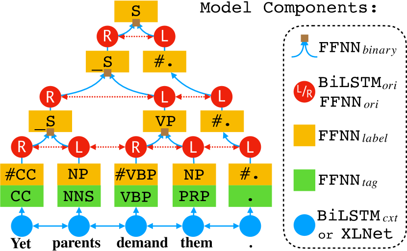
Figure 1: Parsing instance with the binary model. The bottom-up flow of word information is indicated by blue arrows and orientation flows by dotted red arrows. Binary parsing explores the internal constituents of S. Special labels prefixed with “#” or “_” are sub category placeholders caused by binarization and stratification.

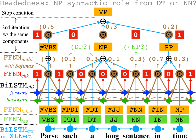
Figure 2: Multi-branching parsing uses chunks instead of orientations to form constituents. Chunks impose Softmax-normalized weights for their inputs. The unsupervised weights provide a shred of evidence for the headedness problem Zwicky (1985).

We propose a pair of greedy combinatory parsers (i.e., neural combinators) that efficiently utilize vector compositionality with recurrent components to address the aforementioned issues. Their bottom-up parsing process is a recursive layer-wise loop of classification and vector composition, as illustrated in Figures 1 & 2. Both parsers work on multiple unfolded variable-length layers, iteratively combining vectors until one vector remains. The binary model provides either left or right orientation for each word or constituent, whereas the multi-branching model marks chunks as constituents at their boundaries. Constituent embeddings are composed based on orientations or chunks. Tagging and labeling are directly performed on all composed embeddings, creating the elements for building a tree: tags, labels, and paths. The deterministic and greedy characteristics yield two simple and fast models, and they investigate different linguistic aspects.

The contributions of our study are as follows:

• We propose two combinatory parsers at $O(n)$ average-case complexity with a theoretical $O(n^{2})$ upper bound. The binary parser achieves a competitive F1 score on Penn Treebank. Both models are the fastest and yet more compact than many previous models.

• We extend the proposed models with a recent pre-trained language model, XLNet Yang et al. (2019). These models have higher speeds and are comparable to state-of-the-art parsers.

• The binary model leverages Chomsky normal form (CNF) factors as a training strategy and reflects the branching tendency of a language. The multi-branching model reveals constituent headedness Zwicky (1985) with an attention mechanism.

2 Previous Work

Transition-based parsers.

A transducer takes sequential lexical inputs and produces sequential tree-constructing actions in $O(n)$ time. Although it can perfectly parse formal languages, complex semantics and long dependencies make it difficult to parse natural languages. Informative features Liu and Zhang (2017c); Kitaev and Klein (2020); Yang and Deng (2020), or training and decoding strategies such as dynamic oracles Cross and Huang (2016), reranking Charniak and Johnson (2005), beam search, and ensemble, can increase the accuracy. However, these make the models complex, and the paradigm fails to naturally parallelize actions.

Chart-based parsers.

An exhaustive search algorithm checks every possibility in a triangular chart and finds the optimal tree globally. Recent neural chart parsers have achieved state-of-the-art accuracy Kitaev and Klein (2018); Zhou and Zhao (2019); Mrini et al. (2020); Zhang et al. (2020). Despite their high accuracy, they are comparatively inefficient. Only $2n-1$ of $O(n^{2})$ scoring nodes in the chart contain true constituents; many are filler nodes. Chart parsers are often specially engineered for high-speed decoding. (e.g., using Cython)

Other parsers.

Shen et al. (2018) and Nguyen et al. (2020) proposed local-and-greedy parsers in the top-down splitting style. Their models facilitate divide-and-conquer algorithms that construct the tree based on the magnitude of the splitting scores. A similar way of leveraging concurrent and greedy operations appears in an easy-first parser Goldberg and Elhadad (2010). Sequential labeling Gómez-Rodríguez and Vilares (2018); Wei et al. (2020) is a new active thread that also enables parallelism and fast decoding. Collobert (2011) designed an iterative chunking process for parsing. His work stratifies trees into levels of IOBES prefixed constituent chunking nodes. Similar to ours, his parser works from the bottom levels to higher levels. However, the complexity is fixed at $O(n^{2})$ without any node combinations. All models introduced in this section do not exploit vector compositionality.

3 Neural Combinatory Parsing

3.1 Data and Complexity

Our models require stratified trees to train recurrent layers, and the binary model requires further binarization. Stratification and binarization introduce redundant relaying nodes to the trees.

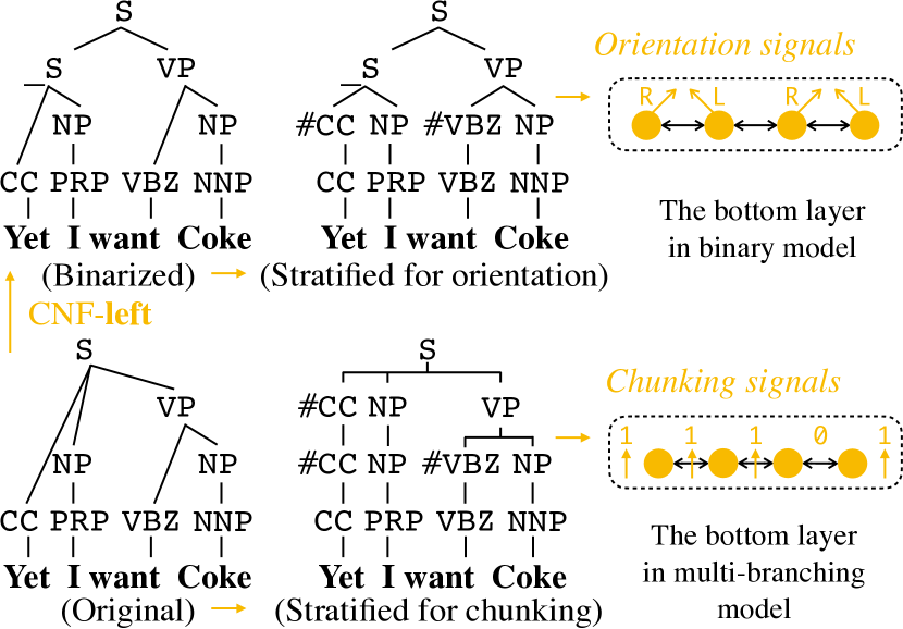
Figure 3: Example illustrating our tree stratification. Both binary and multi-branching stratified trees contain redundancy, from which the original tree can be recovered with a few simple heuristic rules. Four in a layer combine into two with a compression ratio of 1/2.

Tree binarization.

From the bottom-up perspective, a binary tree describes the order in which words and constituents combine with their neighbors into larger constituents, as shown in Figure 3. The orientations of the four words (i.e., right-left-right-left) determine the first combination.

Category	Samples	# Types
Original	S NP VP SBAR+S	$104$
_Sub	_S _NP _VP _PP	$25$
#POS	#NNP #DT #JJ #.	$45$

Table 1: Three categories of our constituent label set with their samples and number of types. This is created from Penn Treebank (PTB). ‘_Sub’ and ‘#POS’ are relaying types, which we group into a sub category.

After binarization, we label the relaying sub-constituents with the parent label prefixed with an underscore mark. If terminal POS tags do not immediately form constituents, we create relaying placeholders prefixed with a hash mark, as presented in Table 1. Unary branches were collapsed into a single node. Plus marks were used to join their labels (e.g., SBAR+S), and all trace branches were removed. The CNF with either a left or a right factor is commonly used. However, it is heuristically biased, and trees can be binarized using other balanced splits such as always splitting from the center to create a complete binary tree (mid-out) and iteratively performing left and right to create another balanced tree (mid-in). Finally, the orientation is extracted from the paths of these binary trees.

CNF	Left-factoring		Right-factoring
Ori.	Left	Right	Left	Right
PTB	3.8M	4.4M	2.3M	6.5M
CTB	2.5M	1.7M	1.4M	2.8M
KTB	4.5M	0.9M	1.8M	2.1M
nCNF	Midin-factoring		Midout-factoring
PTB	3.0M	5.3M	2.8M	5.2M
CTB	1.9M	2.2M	1.7M	2.1M
KTB	2.8M	1.7M	2.5M	1.2M

Table 2: Frequencies of orientation with different CNF (biased) and non-CNF (balanced) factors in different stratified corpora.

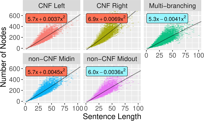
Figure 4: Linear empirical complexity in stratified PTB. Linear regression reflects insignificant $O(n^{2})$ tendencies. We differentiated the quadratic terms with red or light blue colors and omitted the constant biases.

We binarized Penn Treebank (Marcus et al., 1993, PTB) for English, Chinese Treebank (Xue et al., 2005, CTB) for Chinese, and Keyaki Treebank (Butler et al., 2012, KTB) for Japanese to present the syntactic branching tendencies in Table 2. As English is a right-branching language, its majority orientation is to the right. Even left-factoring cannot reverse the trend, but it should create a greater balance. Figure 4 shows that it is less effective to stratify PTB with a right factor because it enhances the tendency. The reverse tendency emerges in the KTB corpus as Japanese is a left-branching language. For Chinese, CTB does not exhibit a clear branching tendency. Non-CNF factors preserve the original tendency.

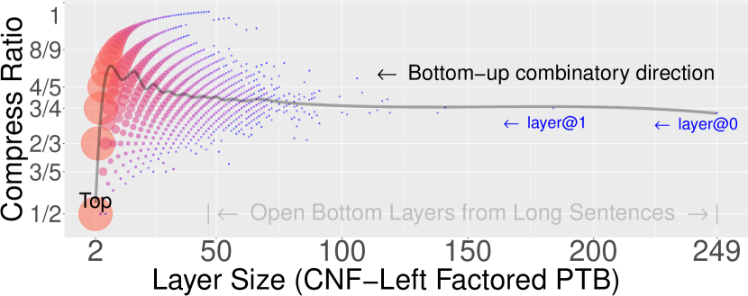
Figure 5: Layer-wise compression ratio over different sizes. The dot size was proportional to the situation count. Statistically, the ratio had a stable mean of 0.77.

Complexity.

Our models are trained with stratified treebanks. The complexity for inference follows the total number of nodes in each layer of a tree. There are two ideal cases: 1) Complete balanced trees with complexity $O(n)$. They contain multiple independent phrases and enable full concurrency. 2) Trees with a single dependency core. The model reduces a constant number of nodes in each layer, resulting in $O(n^{2})$ complexity.

While each parse is a mixture of many cases, the empirical complexity prefers the first case. Formally, the average-case complexity can be inferred as $O(n)$ with the help of a stable compression ratio $0<C<1$ ($C\geq 0.5$ for binary). Let $m_{i}$ represent the number children of the $i$-th tree in a general layer; the compression ratio can be stated as $C=\frac{\sum_{i}1}{\sum_{i}m_{i}}$. Our stratified treebanks give stable $C$s for layers of different lengths, as shown in Figure 5. For the $k$-th layer of a sentence with $n$ words, the number of nodes to compute can be expected to be $C^{k}\cdot n$. Based on tree height $K>0$, the expected number of total parsing nodes is

$$\sum^{K}_{k=0}C^{k}\cdot n=n\cdot\sum_{k=0}^{\infty}C^{k}-n\cdot\sum_{k=K+1}^{\infty}C^{k}<\frac{n}{1-C}\hbox to0.0pt{.\hss}$$

The partial geometric series determines an empirically linear complexity on average.

Theoretically, the complexity has a quadratic upper bound. The general layer with

$$m_{i}=\begin{cases}M&\text{if }i=j\\ 1&\text{otherwise}\end{cases}$$

entails the second case, where $m_{j}$ is the only $M$-ary branch in each layer. The nodes shape a triangular stratified tree with an $O(n^{2})$ complexity. However, this case is rare, especially for long sentences that should contain several concurrent phrases. Otherwise, regression in Figure 4 should show significant $O(n^{2})$ tendencies. (See Appendix A.1 for more support and examples.)

Data structure.

To summarize the data components of a treebank corpus, we used four tensors of indices for 1) words, 2) POS tags, 3) stratified syntactic labels, 4) stratified orientations, or 5) stratified chunks,

$$\left(x_{0:n},t_{0:n},l^{0:k}_{0:n_{k}},o^{0:k}_{0:n_{k}}\ \mathit{or}\ \,c^{0:k}_{0:n_{k}+1}\right)_{j}\in D,$$

where $n$ is the length of the $j$-th sentence, $k$ indicates the $k$-th layer of the stratified data, and $n_{k}$ is the layer length. “:” indicates a range of a sequence.

3.2 Combinatory Parsing

1 Function PARSE($e_{0:n};\ t_{0:n},\ l^{0:k}_{0:n_{k}},\ o^{0:k}_{0:n_{k}}$ or   $c^{0:k}_{0:n_{k}+1}$):

2      $x_{0:n}^{0}\leftarrow$ BiLSTM_cxt($e_{0:n}$)

3      for $i\leftarrow 0$ to $n-1$ do

4           $\hat{t}_{i}\leftarrow$ FFNN _tag($x_{i}^{0}$)

5           $L_{tag}\leftarrow$ CROSS-ENTROPY($t_{i},\hat{t_{i}}$)

6          

7     for $j\leftarrow 0$ to $k$ do

8           for $i\leftarrow 0$ to $n_{j}-1$ do

9                $\hat{l}_{i}^{j}\;\leftarrow$ FFNN _label($x_{i}^{j}$)

10                $L_{label}\leftarrow$ CROSS-ENTROPY($l_{i}^{j},\hat{l}_{i}^{j}$)

11               

12          $x_{0:n_{j+1}}^{j+1}\leftarrow$ COMPOSE($x^{j}_{0:n_{j}};\ o^{j}_{0:n_{j}}\ \mathit{or}\ \,c^{j}_{0:n_{j}+1}$)

13          

14     return $\hat{t}_{0:n},\hat{l}^{0:k}_{0:n_{k}}$

15     

Algorithm 1 Combinatory Parsing

Our models comprise four feedforward (FFNN) and two bidirectional LSTM (BiLSTM) networks to decompose parsing into collaborative functions, as shown in Algorithm 1. During training, we use teacher forcing. In the inference phase, the supervised signals behind all semicolons are ignored; the predicted signals serve as their substitute.

Input $e_{0:n}$ is an embedding sequence indexed by $x_{0:n}$. In lines 2–5, the model prepares a contextual sequence for the combinator and predicts the lexical tags. Lines 6–10 describe the layer-wise loop of the combinator.

The tagging and labeling functions, FFNN_tag and FFNN_label, are 2-layer FFNNs. Their first layer is shared, creating a hidden layer necessary for projecting diversified situations in the manifold to the non-zero logits for the argmax decision. The core function COMPOSE is either a binary Algorithm 2 or a multi-branching Algorithm 3.

1 Function COMPOSE($x_{0:n_{j}}^{j};\ o_{0:n_{j}}^{j}$):

2      $h_{0:n_{j}}^{j}\leftarrow$ BiLSTM_ori($x_{0:n_{j}}^{j}$)

3      for $i\leftarrow 0$ to $n_{j}-1$ do

4           $\hat{o}_{i}^{j}\>\leftarrow$ FFNN_ori($h_{i}^{j}$)

5           $L_{ori}\leftarrow$ HINGE-LOSS($o_{i}^{j},\hat{o}_{i}^{j}$)

6           if $i>0$ and $\hat{o}_{i-1}^{j}+(1-\hat{o}_{i}^{j})>0$ then

7                Append BINARY($\hat{o}_{i-1}^{j},\hat{o}_{i}^{j},\ x_{i-1}^{j},x_{i}^{j}$) to $x^{j+1}$

8               

9          

10     return $x_{0:n_{j+1}}^{j+1}$

11     

12 Function BINARY($o_{L},o_{R},\ x_{L},x_{R}$):

13      if $o_{L}+(1-o_{R})=1$ then // relay

14           return $o_{L}\cdot x_{L}+(1-o_{R})\cdot x_{R}$

15          

16     else  // vector interpolation

17           $\lambda\leftarrow\sigma$ FFNN_binary($x_{L}\oplus x_{R}$)

18           return $\lambda\odot x_{L}+(1-\lambda)\odot x_{R}$

19          

20     

Algorithm 2 Binary Compose

Binary model.

In Algorithm 2, the orientation function is hinted by BiLSTM_ori. A single-layer FFNN_ori with a threshold reduces the outputs to an integer of either 0 or 1 to indicate two possible orientations. In function BINARY, when two adjacent orientations agree as they sum to 2, their embeddings are combined by a combinatory operation. $\sigma$ is the Sigmoid function, “$\oplus$” represents concatenation, and “$\odot$” represents pointwise multiplication. (See Appendix A.3 for more binary variants.)

1 Function COMPOSE($x_{0:n_{j}}^{j};\ c_{0:n_{j}+1}^{j}$):

2      $\vec{h}_{0:n_{j}}^{j},\reflectbox{$\vec{\reflectbox{$h$}}$}_{0:n_{j}}^{j}\leftarrow$ BiLSTM_chk($x_{0:n_{j}}^{j}$)

3      Pad $\vec{h}_{0:n_{j}}^{j}$ with $\vec{h}^{j}_{-1}$ and $\reflectbox{$\vec{\reflectbox{$h$}}$}_{0:n_{j}}^{j}$ with $\reflectbox{$\vec{\reflectbox{$h$}}$}^{j}_{n_{j}}$

4      for $i\leftarrow 0$ to $n_{j}$ do

5           $\hat{c}_{i}^{j}\>\leftarrow$ FFNN _chk($\vec{h}_{i-1}^{j}\oplus\reflectbox{$\vec{\reflectbox{$h$}}$}_{i}^{j}$)

6           $L_{chk}\leftarrow$ HINGE-LOSS($c_{i}^{j},\hat{c}_{i}^{j}$)

7           if $\hat{c}_{i}^{j}=1$ then Append $i$ to $s$ // segment

8               

9           if $i<n_{j}$ then

10                $d^{j}_{i}\leftarrow$ $(\vec{h}^{j}_{i}-\vec{h}^{j}_{i-1})\oplus(\reflectbox{$\vec{\reflectbox{$h$}}$}^{j}_{i}-\reflectbox{$\vec{\reflectbox{$h$}}$}^{j}_{i+1})$

11               

12          

13     for $i\leftarrow 0$ to $|s|-1$ do

14           Append MULTI($d^{j}_{s_{i}:s_{i+1}},\ x^{j}_{s_{i}:s_{i+1}}$) to $x^{j+1}$

15          

16     return $x_{0:n_{j+1}}^{j+1}$

17     

18 Function MULTI($d_{chk},\ x_{chk}$):

19      $\lambda_{chk}\leftarrow\mathit{Softmax}($ FFNN_multi($d_{chk}$)$)$

20      return $\sum_{i}^{chk}\lambda_{i}\odot x_{i}$

Algorithm 3 Multi-branching Compose

Multi-branching model.

To resemble binary interpolation, we use the Softmax function for each chunk, as described in Algorithm 3. BiLSTM_chk is in place of BiLSTM_ori to hint FFNN_chk emitting chunk signals. Segment $s$ splits $x^{j}_{0:n_{j}}$ and $d^{j}_{0:n_{j}}$ into chunks of $x_{chk}$ and $d_{chk}$. FFNN_multi and Softmax turn $d_{chk}$ into attention $\lambda_{chk}$ to interpolate vector chunk $x_{chk}$. Binary interpolation $\lambda$ is a special case of the multi-branching $\lambda_{chk}$ because Sigmoid and Softmax functions are closely related.

To obtain the final tree representation, we apply a symbolic pruner in the same bottom-up manner to remove redundant nodes, expand the collapsed nodes, and assemble the sub-trees based on the neural outputs. (See Appendix A.4.)

4 Experiments

We follow previous data splits for PTB, CTB, and KTB (See Appendix A.2). The preprocessing of data is described in Section 3.1.

For the binary model, we explored interpolated dynamic datasets by sampling two CNF factored datasets. This is because of the following: 1) The experiments with the non-CNF factors did not yield any promising results; thus, we have not reported them. 2) The language was loosely left-branched, right-branched, or did not show a noticeable tendency. Moreover, the use of a single static dataset may introduce a severe orientation bias. 3) All factors are intermediate variables and equally correct. We defined the sampling strategies with two static CNF-factored datasets at certain ratios and named each strategy in the format “L%R%” according to the ratio percentages. Our experiments mainly focus on binary model B because of the aforementioned property for training parsers more accurate than multi-branching model M.

Our parsers do not contain lexical information components Liu and Zhang (2017c); Kitaev and Klein (2018). Instead, we use fastText Bojanowski et al. (2017) because we can obtain pre-trained models easily for many languages or train new ones from scratch with the corpora at hand. We examined its influence in Section 4.2, whereas the official pre-trained embeddings are the default.

Meanwhile, pre-trained language models are useful for various tasks, including constituency parsing Kitaev and Klein (2018, 2020); Zhou and Zhao (2019); Yang and Deng (2020); Mrini et al. (2020). We chose XLNet Yang et al. (2019) to compare with the static fastText embeddings. Specifically, either a 1-layer FFNN (/0) or an $n$-layer BiLSTM (/$n^{+}$) was used to convert the 768-unit output to our model size. We used a GeForce GTX 1080 Ti with 11 GB and a TITAN RTX with 24GB memory only for tuning XLNet.

The model size for vector compositionality was set at 300. The hidden sizes for labeling, orientation, and chunking were 200, 64, and 200, respectively. Different numbers of layers of the BiLSTM_cxt (/$n$) were explored, and the default was six layers. HINGE-LOSS was the default criterion for orientation while binary cross-entropy (BCE-LOSS) was tested. The coefficients of the three losses were explored and the default were $L=0.2\cdot L_{tag}+0.3\cdot L_{label}+0.5\cdot L_{ori\ (\mathbf{or}\ chk)}$.

4.1 Overall Results

Corpus	Penn Treebank					Chinese Treebank
Single Model	Type	sents/sec	LP	LR	F1	Type	LP	LR	F1
Watanabe and Sumita (2015)	T$\uparrow$ (32)	-	-	-	90.7	T$\uparrow$ (64)	-	-	84.3
Gómez-Rodríguez and Vilares (2018)	O	898	-	-	90.7	O	-	-	83.1
Cross and Huang (2016)	T$\uparrow$ (1)	-	92.1	90.5	91.3	-	-	-	-
Liu and Zhang (2017c)	T$\downarrow$ (16)	79.2	92.1	91.3	91.7	T$\downarrow$ (16)	85.9	85.2	85.5
Stern et al. (2017)	C	75.5	93.0	90.6	91.8	-	-	-	-
Shen et al. (2018)	O$\downarrow$ (1)	111.1	92.0	91.7	91.8	O$\downarrow$ (1)	86.6	86.4	86.5
Charniak and Johnson (2005)	C	-	-	-	92.1	-	-	-	-
Ours (multi-branching)	O$\uparrow$ (1)	1122.6	92.1	92.1	92.1	O$\uparrow$ (1)	86.0	84.7	85.3
Ours (binary)	O$\uparrow$ (1)	1327.2	92.8	92.3	92.5	O$\uparrow$ (1)	85.8	86.2	86.0
Nguyen et al. (2020)	O$\downarrow$ (1)	130.2	92.8	92.8	92.8	-	-	-	-
Kitaev and Klein (2018)	C	212.5	93.9	93.2	93.6	C	91.9	91.5	91.7
Wei et al. (2020)	O$\downarrow$ (1)	155	94.1	93.3	93.7	O$\downarrow$ (1)	89.9	87.4	88.7
Zhou and Zhao (2019)	C	226.3	93.9	93.6	93.7	C	92.3	92.0	92.2
Zhang et al. (2020)	C	1092	94.2	94.0	94.1	C	89.7	89.9	89.8

Table 3: Single-model results on PTB and CTB test datasets sorted by the F1 scores on PTB. Transition-based parsers, chart parser, and others are marked as T, C, and O, respectively; $\uparrow$ and $\downarrow$ denote bottom-up and top-down. The number in brackets indicates the beam size. Kitaev and Klein (2018) used Tesla K80, and the CTB scores are cited from Kitaev et al. (2019). Zhou and Zhao (2019) used GeForce GTX 1080 Ti (same condition).

Table 3 lists the parsing accuracies and speeds of the single models in ascending order according to their F1 scores for the PTB corpus. The transition-based parsers with $O(n)$ complexity appear at the top of the table, followed by other types of models, and the chart parsers running in $O(n^{3})$ time are at the bottom of the table. The models exhibited similar trends for the CTB. Shen et al. (2018) and our models belong to type O and have similar complexities. Generally, the accuracy follows the complexity, whereas the speed roughly follows the year of publication rather than complexity or type.

4.2 Comparison of Models

Var	Specification	F1
B/e	without fastText initialization.	91.73
B/$\epsilon$	with tuned official fastText.	91.69
B/E	with frozen fastText from PTB.	92.31
B/F	BiLSTMori into FFNN${}^{\star}_{ori}$.	88.97
B/L	BiLSTMori with BCE-LOSS.	92.32

Table 4: Results of ablation studies on fastText (top) and BiLSTM_ori (bottom) of the binary model.

Models with fastText.

We investigated the binary model through ablation. The impacts of fastText are presented in the upper part of Table 4. B/E does not require any external data beyond PTB, which is comparable to models without a pre-trained GloVe Pennington et al. (2014).

Then, we replaced BiLSTM_ori with an FFNN to examine its effect. The results are in the bottom rows. The comparison proves whether the embeddings are collaborative for the orientation signals because FFNN regards each input independently.

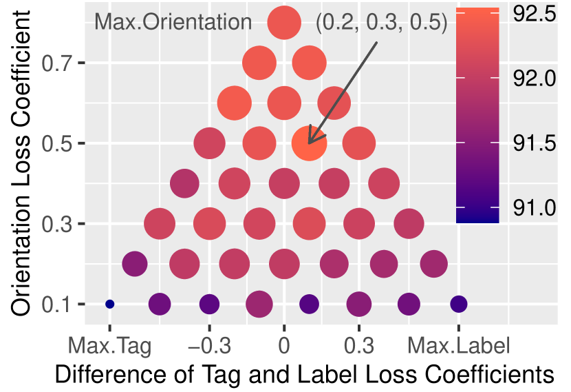
Figure 6: Grid search with an interval of 0.1 in a space of (tag, label, orientation) loss coefficients. The best was (0.2, 0.3, 0.5) indicated by an arrow.

Finally, we used a grid search to explore the hyperparameter space of our three-loss coefficients. Figure 6 shows that the performance correlates to the orientation loss the most, but it is not overly sensitive to the hyperparameters.

	Frozen fastText		Frozen XLNet
Var	F1	sents/sec	F1	sents/sec
B/0	65.02	1386.6	89.24	411.2
B/2	91.34	1350.0	93.74	398.4
B/6	92.54	1327.2	93.89	382.7

Table 5: Effectiveness of using frozen static word embeddings or dynamic sub-word language model and corresponding peak speed.

Pre-trained language model.

We compared the results using frozen fastText with those using frozen XLNet in Table 5. The accuracy of the model increased along with the depth of BiLSTM_cxt, and it exhibited the most significant increase across all variants. Owing to XLNet, our complexities grew to $O(n^{2})$.

Fine-Tuned Model	F1	sents/sec	Type
Kitaev and Klein (2018)	95.13	70.8	C
Kitaev and Klein (2020)	95.44	1200	T
Nguyen et al. (2020)	95.48	-	O$\downarrow$
Zhang et al. (2020)	95.69	-	C
Wei et al. (2020)	95.8	-	O$\downarrow$
Zhou and Zhao (2019)	96.33	64.8	C
Yang and Deng (2020)	96.34	71.3	T
Mrini et al. (2020)	96.38	59.2	C
B/0 (XLNet+FFNN)	95.72	411.2	O$\uparrow$
B/2 (XLNet+BiLSTM)	94.67	398.4	O$\uparrow$
M/0 (XLNet+FFNN)	95.44	369.4	O$\uparrow$

Table 6: Improvements with pre-trained language models. We used a greedy search algorithm on single GeForce GTX 1080 Ti. Rows 6–8 are reported by Yang and Deng (2020) using GeForce GTX 2080 Ti. Kitaev and Klein (2020) used a cloud TPU with a beam search algorithm and a larger batch size.

We fine-tuned our models and compared them with other parsers using fine-tuned language models. These are listed in Table 6.

4.3 Tree-Binarization Strategy

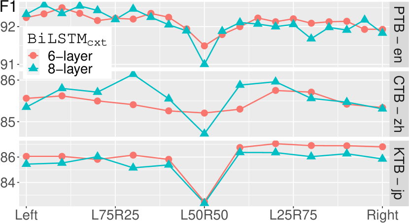
Figure 7: Probabilistic interpolations of two CNF factors to F1 scores. The capacity of BiLSTM_cxt is almost saturated with 6 or 8 layers.

To reflect the branching tendency, our best single model for PTB was obtained on the dynamic L95R05 dataset. This dataset is a probabilistic interpolation between the left-factored dataset (for 95% chances) and a right-factored dataset (for 5% chances) in Figure 7. The best model for CTB appeared on the left side at L70R30, scoring $86.14$, whereas the best for KTB was on the L30R70 dataset, scoring $87.05$ with a 6-layer BiLSTM_cxt. Typically, the results for all the corpora had a minimum at L50R50. For English, the left “wing” was higher than the right; the opposite trend was observed for Japanese. For Chinese, no clear trend was obtained.

All studies described in the previous sections were conducted on the PTB L85R15 dataset.

4.4 Complexity and Speed

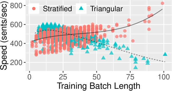
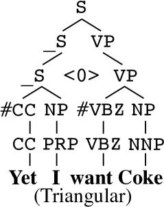
Figure 8: Linear complexity vs. squared complexity. Redundancy with placeholder “<0>” helps maintain the triangular shape.

Format	Time/150	Memory	OOM
Stratified	7.5 hours	3.3 GB	-
Triangular	15.9 hours	8.2 GB	100

Table 7: Training time and memory consumed by our two data formats. The time column indicates the time used for 150 training epochs with validations. Development F1 scores are approximately 92.4. The OOM column lists the length limit for preventing an out-of-memory error. Kitaev and Klein (2018) took 10 hours for 93 training epochs on our GeForce GTX 1080 Ti to yield their results.

To test our linear speed advantage, we inflated our training data with redundant nodes to resemble the triangular chart of CYK algorithm, as depicted in Figure 8 and Table 7. The parse in the triangular treebank has the worst-case complexity of $O(n^{2})$. Meanwhile, training with linearity halved the training time, reduced memory usage, and canceled the length limit for our three corpora. There is a sheer difference between linearity and squared complexity.

5 Discussion

5.1 Model Structure

Our parsers comprise a neural encoder for scoring (i.e., Algorithm 1) and a non-neural decoder for searching. The decoder is a symbolic extension of the encoder in that both run in bottom-up manner, and the decoder interprets the scores as local-and-greedy decisions. Other neural parsers also fit a similar encoder–decoder framework. However, decoders with dynamic programming often include forward and backward processes heterogeneous to their forward encoders Kitaev and Klein (2018, 2020). The encoder and decoder in our model and Shen et al. (2018) are more homogeneous and can be easily merged. Our parsers are bottom-up combinatory, while theirs was top-down splitting. Similar homogeneity can be found in an easy-first dependency parser Goldberg and Elhadad (2010).

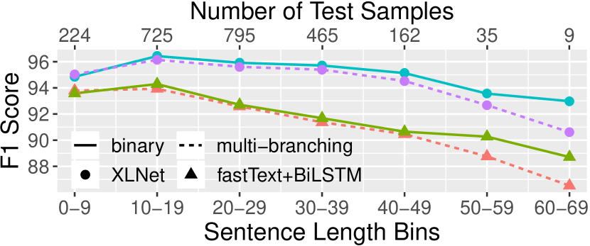
Figure 9: XLNet provides an overall improvement for all models and length bins. All models find it challenging to handle long sentences.

Input component.

In terms of encoder, Tables 4–6 examine the impact of BiLSTM_cxt with fastText or XLNet, and the following conclusions can be drawn. 1) The top rows of Table 4 suggest that frozen fastText embeddings contain sub-word information, whereas tuning them disturbs the frozen information because the n-gram model is not part of our model. 2) Table 5 shows that the deeper the contextualization BiLSTM_cxt (or XLNet), the better the results. 3) Tables 5 and 6 indicate that the tuning process for the pre-trained language models Peters et al. (2018); Devlin et al. (2019); Yang et al. (2019) achieves a significant improvement.

Speed and size.

One of our research goals was to achieve simplicity and efficiency. In terms of speed, our models parallelize more actions than transition-based parsers and have fewer computing nodes than chart parsers. In terms of size, our models contain approximately 4M parameters in addition to the 13M fastText (or 114M XLNet) pre-trained embeddings, which is fewer than those of Shen et al. (2018, 22M+) and Kitaev and Klein (2018, 26M). The recursiveness and productiveness of vector compositionality should account for the compact size.

Vector compositionality.

The performance of FFNN${}_{ori}^{\star}$ is inferior to that of its RNN counterparts, suggesting that some information might not be encoded locally. Thus, the COMPOSE function should remain in a contextual form to collaboratively leverage the whole layer. However, BiRNN might still be a bottleneck for long-range orientation, as suggested in Figure 9. BiLSTM_chk is a major weakness of the multi-branching model, especially for longer sentences.

5.2 Tree Binarization and Headedness

Tree binarization.

Probabilistic interpolation with two CNF-factored datasets is effective for the three languages studied, as shown in Figure 7. Dynamic sampling allows the model to cover a wider range of composed vectors to improve its robustness to ambiguous orientations. Furthermore, it seems counterintuitive for human learners to obtain the best model using left-biased interpolation for a right-branching language or vice versa. However, for a neural model, balancing the frequency seems to be the key factor for improving performance Sennrich et al. (2016); Zhao et al. (2018). The fact that the L50R50 dataset yielded the worst models also suggests that the balance should be based on a default orientation tendency. This could also be the reason why mid-in or mid-out did not improve the model.

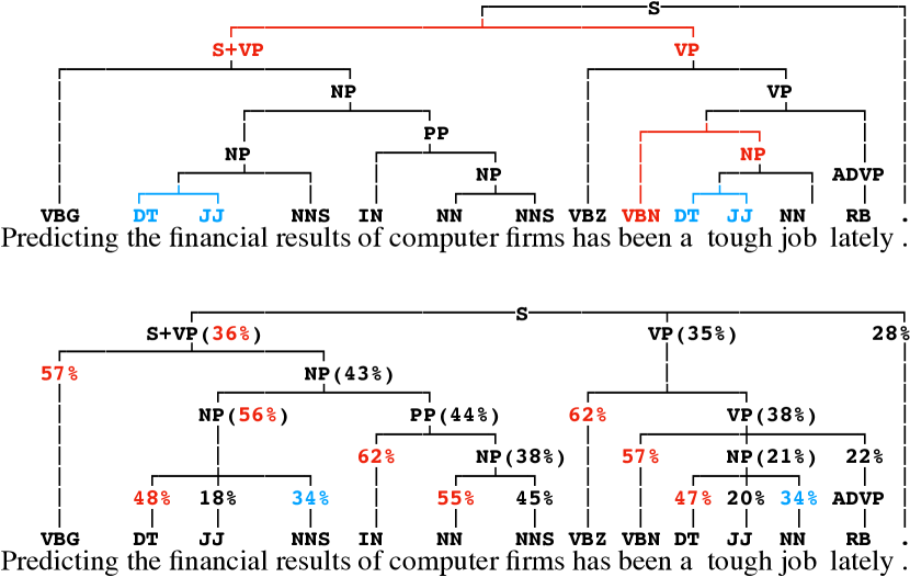
Figure 10: English internal constituents (top) and headedness (bottom) from our two models.

Headedness.

Figure 10 show the intermediate parses on the same sentence from our two models. They are typical examples in the output.

The binary model first combines determiners and their right neighbors rather than adjectives and nouns in noun phrases (blue spans). It also postpones the combination with adjuncts such as punctuation and adverb (red spans). The high frequencies of determiners in noun phrases make them great attractors.

Parent (#)	Head child by maximum weight
NP(14.4K)	DT (4.5K); *NP (4.3K); *NNP (1.6K); *JJ (922); *NN (751); *NNS (616); etc. (1.6K; 38 of 50 types with “*”)
VP(6.8K)	VBD (1.5K); VB (1.4K); VBZ (1.0K); VBN (954); VBP (705); MD (523); VBG (387); VP (169); TO (81); etc.
PP(5.5K)	IN (5.0K); TO (397); etc.
S(3.8K)	VP (3.4K); S (194); NP (90); etc.
SBAR (1.2K)	IN (649); WHNP (395); WHPP (19); WHADVP (121); SBAR (15); etc.
ADVP(278)	RB (181); IN (30); RBR (25); etc.
QP(198)	CD (67); IN (65); RB (29); JJR (16);

Table 8: English headedness selection with our multi-branching model on PTB test set. “*” marks the absence of a DT child for its NP sisters. For quantifier phrases (QP), some non-quantifiers are more likely to be heads if they appear; e.g., adverbs (RB; e.g., “approximately”), prepositions (IN; e.g., “about”), and relative adjectives (JJR; e.g., “more than”).

On the other hand, the multi-branching model places close attention on what the syntactic head is supposed to be. In the noun phrases, determiners receive the highest weight averages (red), and the nouns obtain the second (blue). This phenomenon suggests that an English noun phrase’s syntactic role is mainly projected from the determiners, as discussed by Zwicky (1985). Table 8 provides more statistical support. For example, the model selects DT as an NP head if it is available; otherwise, nouns and adjectives are prominent heads. Chinese and Japanese parsers work similarly for their headedness. (See Appendix A.5.)

5.3 Error Analysis

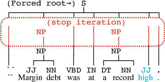
Figure 11: Failed parse from the multi-branching model. The model stops parsing and saves computations when it repeats the same chunking positions.

The rate of an invalid parse is the last topic that we consider for our parsers. For the binary parser, fatal errors, such as frame-breaking orientations, appear at an early stage of training. However, the late $90\%$ of training time contains very few errors, and our binary model is free from invalid parsing on the test set. For the multi-branching parser, it is observed that 11 out of 2,416 test parses are forests rather than parse trees when they are trained with fastText. However, the multi-branching parser with fine-tuned XLNet reduces the error count on the test set to 1.

We present a failed multi-branching parse with fastText, as shown in Figure 11. The postnominal adjective “high” is uncommon for English. Because the model did not group it with the adjacent “a record” to form an NP, the error propagated to higher layers (e.g., no PP as an adjunct to form a VP), causing the bad parse. It implies that the multi-branching model requires an appropriate predict-argument configuration to chunk.

6 Conclusion

We proposed a pair of neural combinatory constituency parsers. The binary one yields F1 scores comparable to those of recent neural parsers. The multi-branching one reveals constituency headedness. Both are simple and efficient with relatively high speeds. We also leveraged a pre-trained language model and CNF factors to increase the accuracy. We reflected the branching tendencies of three languages.

Appendix A Appendices

A.1 Compression Ratios and Linearity

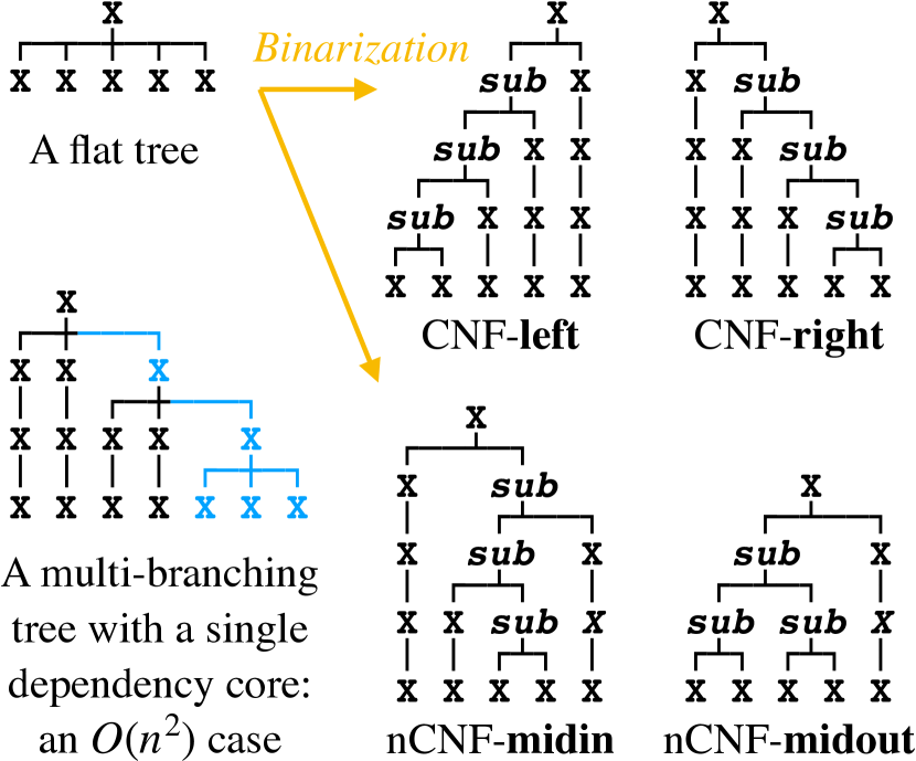
Figure 12: Examples used in the content. A flat tree is binarized with four factors. The binarization of CNF-left, CNF-right, or nCNF-midin creates binary trees with a single dependency core (i.e., a single sub thread), whose $O(n^{2})$ complexity is the same with the tree without binarization in the lower left. Most nodes are relaying nodes. Meanwhile, nCNF-midout enables concurrent phrases with $O(n)$ complexity (i.e., multiple sub threads). However, the division tends to break a constituent into ungrammatical pieces, which confuses the model and does not lead to improvement.

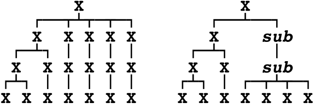
Figure 13: Adding sub nodes to make flat structure more efficient. Using the strategy as a new dynamic dataset also brings multi-branching model M a stable accuracy improvement with an F1 score of 92.36 on PTB. However, it has nothing to do with linguistic properties. We save it for a future study.

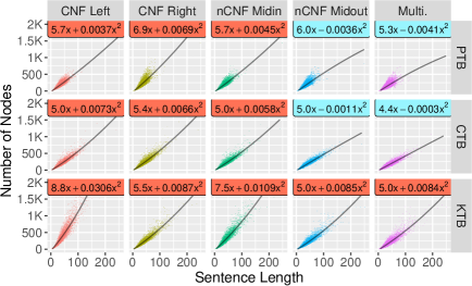
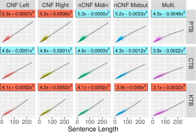
Figure 14: Left: the empirical complexities related to Figures 15 & 16. Linear regressions are shown on a light blue background when the quadratic terms are negative. Right: resultant complexities after a preprocessing that groups the flat structure into sub-constituent before stratification. (See Figure 13.)

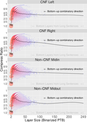
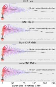
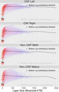
Figure 15: Binarized corpora with four factors. Curved tiers can be observed in each plot. For example, the leftmost tier is composed of $\frac{n-1}{n}$ (followed by $\frac{n-2}{n}$, $\frac{n-3}{n}$, and so on). The dots in this tier range from a high compression ratio of 0.5 to the least efficient ones in their corpus. Efficient dots are more populated, judging by their sizes and colors. All statistics yield stable means, which are also presented in Table 9.

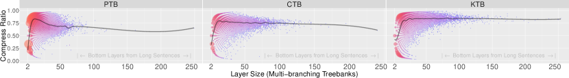
Figure 16: Multi-branching corpora. Curved tiers appear more symmetric and all statistics still yield stable means.

Factor	Left	Right	Midin	Midout	Multi.
All layers
PTB	$0.77\ {\pm 0.11}$	$0.79\ {\pm 0.11}$	$0.78\ {\pm 0.11}$	$0.77\ {\pm 0.11}$	$0.73\ {\pm 0.20}$
CTB	$0.77\ {\pm 0.11}$	$0.77\ {\pm 0.11}$	$0.76\ {\pm 0.11}$	$0.74\ {\pm 0.11}$	$0.70\ {\pm 0.20}$
KTB	$0.82\ {\pm 0.12}$	$0.75\ {\pm 0.12}$	$0.79\ {\pm 0.12}$	$0.73\ {\pm 0.12}$	$0.69\ {\pm 0.29}$
Layers longer than 40
PTB	$0.78\ {\pm 0.04}$	$0.80\ {\pm 0.04}$	$0.77\ {\pm 0.04}$	$0.74\ {\pm 0.04}$	$0.69\ {\pm 0.08}$
CTB	$0.79\ {\pm 0.04}$	$0.80\ {\pm 0.04}$	$0.78\ {\pm 0.04}$	$0.77\ {\pm 0.04}$	$0.76\ {\pm 0.07}$
KTB	$0.90\ {\pm 0.04}$	$0.80\ {\pm 0.05}$	$0.86\ {\pm 0.04}$	$0.77\ {\pm 0.06}$	$0.84\ {\pm 0.07}$

Table 9: Mean and standard deviation of compression ratios of Figures 15 & 16. Longer layers have converged deviations. The last column came from the multi-branching treebanks without a binarizing factor.

Figure 12 presents examples for tree binarization and the worst case of $O(n^{2})$ complexity. Figure 14 shows the overall linear data complexities in the three languages. Figures 15 & 16 and Table 9 indicate that, given a language and a factor, the compression ratio is stable and seldom affected by the sentence length.

The regressions for PTB and CTB show weak $O(n^{2})$ tendencies; the quadratic coefficients can be either positive or negative. Meanwhile, KTB falls into the worst case, as shown in Figure 14. This is because KTB trees tend to have a flat structure on the right side of parses, as illustrated in Figure 17. Relaying nodes in the flat structure never combine until the final layer, creating strong $O(n^{2})$ tendencies. As a result, all KTB datasets fall into the worst case, especially when binarized with the CNF-left factor.

A preprocess that groups the flat structure into the sub category can prevent considerable quadratic impacts on all datasets. All $O(n^{2})$ tendencies are largely weakened across three corpora, and all linear coefficients drop significantly, as illustrated on the right of Figure 14. The preprocess cannot eradicate the worst case in KTB. However, all linear coefficients’ magnitudes are at least hundreds of times larger than those of the quadratic terms. In our sub-quadratic case, 200 words lead to approximately 1.5K nodes. Meanwhile, a sentence with $n$ words has a triangular chart with $\frac{n(n+1)}{2}$ nodes, whose quadratic coefficient is 0.5. In this case, 200 words lead to approximately 20K nodes.

A.2 Experiment Setting

The treebanks PTB and CTB have been widely used for experiments. For PTB, sections 2-21 were used for training, section 22 for development, and section 23 for testing. For CTB, articles 001-270 and 440-1151 were used for training, 301-325 for development, and 271-300 for testing. There is no widely accepted data split for the KTB corpus, except for some probabilistic divisions, because KTB contains mixed data from sources such as newswires, book digests, and Wikipedia. We randomly reserved 2,075 samples for development, 1,863 samples for testing, and the remaining 3.3 million as training samples. Few sentences in the training sets were longer than 100 words (3 of 40K in PTB; 96 of 17K in CTB; 55 of 33K in KTB). Frozen English (wiki.en.bin), Chinese (cc.zh.300.bin), and Japanese (cc.ja.300.bin) embeddings were used for PTB, CTB, and KTB, respectively. We fed fastText with the PTB text to train cbow instead of skipgram embeddings for B/E with their default settings for 50 epochs.

The batch size was 80, and sentences longer than 100 words were excluded for the triangular data to avoid out-of-memory (OOM) errors on a single GeForce GTX 1080 Ti with 11 GB. We froze XLNet to train our model and then tuned XLNet from the 5-th epoch. We doubled the batch size at the inference phase to 160.

We used the Adam optimizer with a default learning rate of $10^{-3}$, while we opted for the XLNet’s Adam hyperparameters when tuning the pre-trained XLNet (e.g., their learning rate was $10^{-5}$). We adopted a warm-up period for one epoch and a linear decrease after the 15-th decrease since the last best evaluation. The recurrent dropout rate was 0.2; other dropout probabilities for FFNNs were set to 0.4. For model selection, the training process terminated when the development set did not improve above the highest score after 100 consecutive evaluations. The Evalb program was used for F1 scoring.

Input		Development		Test
Comp.	M.	F1	$P-R$	F1	$P-R$
Frozen	B	92.50	0.00	92.54	$+$0.56
fastText	M	92.10	$-$0.35	92.10	$-$0.03
Tuned	B	95.64	$-$0.05	92.72	$+$0.19
XLNet	M	95.34	$-$0.15	92.44	$+$0.30

Table 10: F1 scores and differences in precision and recall ($P-R$) on the PTB development and test sets.

We demonstrated score profiles for our main models in Table 10. The discrepancy in F1 scores and difference between precision and recall are relatively small on the PTB development and test sets.

A.3 Variants of Binary Compose

1 Function BINARY($o_{L},o_{R},\ x_{L},x_{R};\text{Var}$):

2       $x\leftarrow o_{L}\cdot x_{L}+(1-o_{R})\cdot x_{R}$

3       if $o_{L}+(1-o_{R})=1$ then // relay

4             return $x$

5            

6      else if Var is ADD then // ADD

7             return $x$

8            

9       else

10             if Var is NS or NV then // No input

11                   $\lambda\leftarrow\sigma$ FFNN_binary($\emptyset$)

12                  

13            else if Var is CS or CV then // Concat$\dots$

14                   $\lambda\leftarrow\sigma$ FFNN_binary($x_{L}\oplus x_{R}$)

15                  

16            else if Var is BV then // Biaffine

17                   $\lambda\leftarrow\sigma$ FFNN_binary($x_{L},x_{R}$)

18                  

19             if Var is NV, CV, or BV then // Vector $\lambda$

20                   $x\leftarrow\lambda\odot x_{L}+(1-\lambda)\odot x_{R}$

21                  

22             else if Var is NS or CS then // Scalar $\lambda$

23                   $x\leftarrow\lambda\cdot x_{L}+(1-\lambda)\cdot x_{R}$

24                  

             return $x$

              // NS NV CS CV BV

25            

26      

Algorithm 4 Binary Compose Variants

If we choose the relay instruction in line 12 of Algorithm 2, additive vector compositionality is retained Mikolov et al. (2013) as the naïve ADD variant in lines 5–6 of Algorithm 4. The model can infer a full tensor tree; however, ADD causes the vector magnitude to increase with the tree height cumulatively. This is unwanted in the recurrent or recursive neural network.

Therefore, we examined a learnable FFNN_multi with Sigmoid activation to perform gate-style interpolation in five variants NS, NV, CS, CV, and BV as described in lines 8–17. When a variant takes no input and produces a scalar interpolation parameter $\lambda$, we consider this case NS. (“$\varnothing$” is a placeholder for no input.) Meanwhile, CV indicates concatenated input and vectorized interpolation. BV is a variant that involves a biaffine tensor operation. CV is our default BINARY variant; the experiments for these variants are presented in Table 11.

Var	Specification	F1
BV	Biaffine inputs for vector $\lambda$.	92.53
CV	$x_{L}\oplus x_{R}$ as input for vector $\lambda$.	92.54
CS	$x_{L}\oplus x_{R}$ as input for scalar $\lambda$.	91.83
NV	No input; bias vector $\lambda$.	92.36
NS	No input; bias scalar $\lambda$.	91.95
ADD	$x_{L}+x_{R}$	91.86

Table 11: Compositionality of the BINARY function.

In terms of the F1 score, the most competitive variants of CV are BV and NV, suggesting that fine interpolation can effectively facilitate vector compositionality. The similarity in results of CS, NS, and ADD validate this suggestion. This indicates that vector compositionality is not as trivial as an additive function at the scalar level, and a matrix operation is sufficient. BV is the costliest variant with a tensor operation that runs very slowly (30 sents/sec).

A.4 Recovering Symbolic Tree

1 Function REC($x_{0:n},\ t_{0:n},\ l^{k}_{0:n_{k}},\ o^{k}_{0:n_{k}}\ or\ c^{k}_{0:n_{k}+1}$):

2      for $i\leftarrow 0$ to $n-1$ do

3           $tree_{i}\leftarrow$ TREE($t_{i},x_{i}$)

4          

5     for $j\leftarrow 0$ to $k-2$ do

6           if binary parsing then // BINARY

7                for $i\leftarrow 0$ to $n_{j}-1$ do

8                     if $o_{i}^{j}+(1-o_{i+1}^{j})=2$ then

9                          Combine $tree_{i:i+2}$ under $l_{\mathit{parent\_of(i,i+1)}}^{j+1}$

10                         

11                    

12          else // MULTI-BRANCHING

13                foreach $chk\ \mathit{in}\ c^{j}_{0:n_{j}+1}$ do

14                     Combine $tree_{chk}$ under $l_{\mathit{parent\_of(chk)}}^{j+1}$

15                    

16     Expand unary and flatten sub labels for $tree_{0}$

17      return $tree_{0}$

Algorithm 5 Recovering a Symbolic Tree

To obtain the final tree representation, we initialized the working place with leaves of words and predicted POS tags. Two symbolic rules were used to modify the labels and construct sub-trees, as described in Algorithm 5. 1) The collapsed unary branches were expanded to their original structure by splitting at the plus marks (e.g., SBAR+S into SBAR and S). 2) ‘the label is a sub’ excluded the repeated labels and relayed sub-trees. These rules enabled a single $tree_{0}$ as the final output.

A.5 Chinese and Japanese Headedness

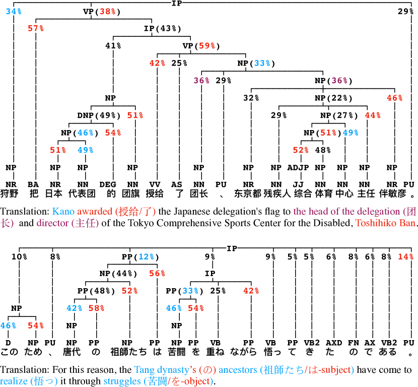
Figure 17: Chinese (top) and Japanese (bottom) parses from the multi-branching model.

Figure 17 presents two non-English parses from the multi-branching model. Both the Chinese and Japanese languages possess functional markers that receive high attention (percentage and words in red), such as the second character tagged with BA in Chinese, and Japanese case markers tagged with PP. Interestingly, the Chinese verb (i.e., the one meaning “awarded”) received the highest attention, whereas Japanese verbs (i.e., two sub-words tagged with VB) did not. We supposed the reason behind this is that Japanese sentences drop the VBs and other heads more often than Chinese. The coordinated NPs in the Chinese parse (i.e., two words meaning “head” and “director”) received equal attention weights.

Moreover, two trees show their branching tendencies: Chinese is midin-alike; Japanese is a left-branching language, and KTB has a large flat structure on the right.

References

- Bahdanau et al. (2015) Dzmitry Bahdanau, Kyunghyun Cho, and Yoshua Bengio. 2015. Neural Machine Translation by Jointly Learning to Align and Translate. In Proceedings of the 3rd International Conference on Learning Representations.
- Bojanowski et al. (2017) Piotr Bojanowski, Edouard Grave, Armand Joulin, and Tomas Mikolov. 2017. Enriching Word Vectors with Subword Information. Transactions of the Association for Computational Linguistics, 5:135–146.
- Butler et al. (2012) Alastair Butler, Tomoko Hotta, Ruriko Otomo, Kei Yoshimoto, Zhen Zhou, and Hong Zhu. 2012. Keyaki Treebank: phrase structure with functional information for Japanese. In Proceedings of Text Annotation Workshop, 2012.
- Charniak (2000) Eugene Charniak. 2000. A Maximum-Entropy-Inspired Parser. In Proceedings of 6th Applied Natural Language Processing Conference, pages 132–139.