Spherical CR uniformization of the magic 3-manifold

Abstract.

We show the 3-manifold at infinity of the complex hyperbolic triangle group $\Delta_{3,\infty,\infty;\infty}$ is the three-cusped magic 3-manifold $6_{1}^{3}$. We also show the 3-manifold at infinity of the complex hyperbolic triangle group $\Delta_{3,4,\infty;\infty}$ is the two-cusped 3-manifold $m295$ in the Snappy Census, which is a 3-manifold obtained by Dehn filling on one cusp of $6_{1}^{3}$. In particular, hyperbolic 3-manifolds $6_{1}^{3}$ and $m295$ admit spherical CR uniformizations.

These results support our conjecture that the 3-manifold at infinity of the complex hyperbolic triangle group $\Delta_{3,n,m;\infty}$ is the one-cusped hyperbolic 3-manifold obtained from the magic manifold $6_{1}^{3}$ via Dehn fillings with filling slopes $(n-2)$ and $(m-2)$ on the first two cusps of it.

1. Introduction

1.1. Motivation

Thurston’s work on 3-manifolds has shown that geometry has an important role to play in the study of topology of 3-manifolds. There is a very close relationship between the topological properties of 3-manifolds and the existence of geometric structures. A spherical CR-structure on a smooth 3-manifold $M$ is a maximal collection of distinguished charts modeled on the boundary $\partial\mathbf{H}^{2}_{\mathbb{C}}$ of the complex hyperbolic space $\mathbf{H}^{2}_{\mathbb{C}}$, where coordinates changes are restrictions of elements of $\mathbf{PU}(2,1)$. In other words, a spherical CR-structure is a $(G,X)$-structure with $G=\mathbf{PU}(2,1)$ and $X=S^{3}$. In contrast to the results on other geometric structures carried on 3-manifolds, there are relatively few examples known about spherical CR-structures.

In general, it is very difficult to determine whether a 3-manifold admits a spherical CR-structure or not. Some of the first examples were given by Burns-Shnider [4]. Three-manifolds with $Nil^{3}$-geometry naturally admit such structures, but by Goldman [11], any closed 3-manifold with Euclidean or $Sol^{3}$-geometry does not admit such structures.

We are interested in an important class of spherical CR-structures, called uniformizable spherical CR-structures. A spherical CR-structure on a 3-manifold $M$ is uniformizable if it is obtained as $M=\Gamma\backslash\Omega_{\Gamma}$, where $\Omega_{\Gamma}\subset\partial\mathbf{H}^{2}_{\mathbb{C}}$ is discontinuity region of a discrete subgroup $\Gamma$ acting on $\partial\mathbf{H}^{2}_{\mathbb{C}}=S^{3}$. Constructing discrete subgroups of $\mathbf{PU}(2,1)$ can be used to constructed spherical CR-structures on 3-manifolds. Thus, the study of the geometry of discrete subgroups of $\mathbf{PU}(2,1)$ is crucial to the understanding of uniformizable spherical CR-structures. Complex hyperbolic triangle groups provide rich examples of such discrete subgroups. As far as we know, almost all known examples of uniformizable spherical CR-structures are relate to complex hyperbolic triangle groups.

Let $\Delta_{p,q,r}$ be the abstract $(p,q,r)$ reflection triangle group with the presentation

$$\langle\sigma_{1},\sigma_{2},\sigma_{3}|\sigma^{2}_{1}=\sigma^{2}_{2}=\sigma^{2}_{3}=(\sigma_{2}\sigma_{3})^{p}=(\sigma_{3}\sigma_{1})^{q}=(\sigma_{1}\sigma_{2})^{r}=id\rangle,$$

where $p,q,r$ are positive integers or $\infty$ satisfying $1/p+1/q+1/r<1$. One can choose the integers so that $p\leq q\leq r$. If $p,q$ or $r$ equals $\infty$, then the corresponding relation does not appear. A complex hyperbolic $(p,q,r)$ triangle group is a representation $\rho$ of $\Delta_{p,q,r}$ into $\mathbf{PU}(2,1)$ where the generators fix complex lines, we denote $\rho(\sigma_{i})$ by $I_{i}$. It is well known that the space of $(p,q,r)$-complex reflection triangle groups has real dimension one if $3\leq p\leq q\leq r$. Sometimes, we denote the representation of the triangle group $\Delta_{p,q,r}$ into $\mathbf{PU}(2,1)$ such that $I_{1}I_{3}I_{2}I_{3}$ of order $n$ by $\Delta_{p,q,r;n}$.

Richard Schwartz has conjectured the necessary and sufficient condition for a complex hyperbolic $(p,q,r)$ triangle group $\langle I_{1},I_{2},I_{3}\rangle<\mathbf{PU}(2,1)$ to be a discrete and faithful representation of $\Delta_{p,q,r}$ [29]. Schwartz’s conjecture has been proved in a few cases.

We now provide a brief historical overview, before discussing our results. Schwartz proved the following theorem, first conjectured by Goldman and Parker [14].

Theorem 1.1 (Schwartz [26, 30]).

Let $\Gamma=\langle I_{1},I_{2},I_{3}\rangle<\mathbf{PU}(2,1)$ be a complex hyperbolic ideal triangle group. If $I_{1}I_{2}I_{3}$ is not elliptic, then $\Gamma$ is discrete and faithful. Moreover, if $I_{1}I_{2}I_{3}$ is elliptic, then $\Gamma$ is not discrete.

Furthermore, he analyzed the group when $I_{1}I_{2}I_{3}$ is parabolic.

Theorem 1.2 (Schwartz [27]).

Let $\Gamma=\langle I_{1},I_{2},I_{3}\rangle$ be the complex hyperbolic ideal triangle group with $I_{1}I_{2}I_{3}$ being parabolic. Let $\Gamma^{\prime}$ be the even subgroup of $\Gamma$. Then the manifold at infinity of the quotient ${\bf H}^{2}_{\mathbb{C}}/{\Gamma^{\prime}}$ is commensurable with the Whitehead link complement in the 3-sphere.

Recently, Schwartz’s conjecture was shown for complex hyperbolic $(3,3,n)$ triangle groups with positive integer $n\geq 4$ in [22] and $n=\infty$ in [23].

Theorem 1.3 (Parker, Wang and Xie [22], Parker and Will [23]).

Let $n\geq 4$, and let $\Gamma=\langle I_{1},I_{2},I_{3}\rangle$ be a complex hyperbolic $(3,3,n)$ triangle group. Then $\Gamma$ is a discrete and faithful representation of the $(3,3,n)$ triangle group if and only if $I_{1}I_{3}I_{2}I_{3}$ is not elliptic.

There are some interesting results on complex hyperbolic $(3,3,n)$ triangle groups with $I_{1}I_{3}I_{2}I_{3}$ being parabolic.

Theorem 1.4 (Deraux and Falbel [8], Deraux [6] and Acosta [1]).

Let $4\leq n\leq+\infty$, and let $\Gamma=\langle I_{1},I_{2},I_{3}\rangle$ be a complex hyperbolic $(3,3,n)$ triangle group with $I_{1}I_{3}I_{2}I_{3}$ being parabolic. Let $\Gamma^{\prime}$ be the even subgroup of $\Gamma$. Then the manifolds at infinity of the quotient ${\bf H}^{2}_{\mathbb{C}}/{\Gamma^{\prime}}$ is obtained from Dehn surgery on one of the cusps of the Whitehead link complement with slope $n-2$.

Note that the choice of the meridian-longitude systems of the Whitehead link complement in Theorem 1.4 is different from that in [1]. The meridian-longitude systems chosen here is from [19], which seems more coherent for the manifolds at infinity of the complex hyperbolic triangle group $\Delta_{3,m,n;\infty}$ below.

These deformations furnish some of the simplest interesting examples in the still mysterious subject of complex hyperbolic deformations. While some progress has been made in understanding these examples, there is still a lot unknown about them.

1.2. Our result

The main purpose of this paper is to study the geometry of triangle groups $\Delta_{3,\infty,\infty;\infty}$ and $\Delta_{3,4,\infty;\infty}$. Thompson showed [25] that $\Delta_{3,\infty,\infty;\infty}$ and $\Delta_{3,4,\infty;\infty}$ are arithmetic subgroups of $\mathbf{PU}(2,1)$, thus they are discrete. We will identify the manifolds at infinity for them via Ford domains. Our main results are the following Theorems 1.5 and 1.6. Theorem 1.5 is also step one of a possible approach to Conjecture 1.7 later.

Theorem 1.5.

Let $\Gamma=\langle I_{1},I_{2},I_{3}\rangle$ be the complex hyperbolic triangle group $\Delta_{3,\infty,\infty;\infty}$. Then the manifold at infinity of the even subgroup $\langle I_{1}I_{2},I_{2}I_{3}\rangle$ of $\Gamma$ is the magic 3-manifold $6_{1}^{3}$ in the Snappy Census.

Theorem 1.6.

Let $\Gamma=\langle I_{1},I_{2},I_{3}\rangle$ be the complex hyperbolic triangle group $\Delta_{3,4,\infty;\infty}$. Then the manifold at infinity of the even subgroup $\langle I_{1}I_{2},I_{2}I_{3}\rangle$ of $\Gamma$ is the two-cusped hyperbolic 3-manifold $m295$ in the Snappy Census.

The magic 3-manifold is the complement of the simplest chain link in $\mathbb{S}^{3}$ with three components [19], which appears as $6_{1}^{3}$ in Rolfsen’s list [24], and it is a hyperbolic 3-manifold [5]. Note also that $m295$ is the two-components link $9^{2}_{50}$ in Rolfsen’s list [24]. See Figure 1 for the diagrams of these two links in the 3-sphere.

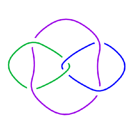
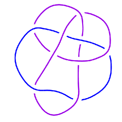
Figure 1. Left: the magic 3-manifold $6_{1}^{3}$. Right: the two-cusped 3-manifold $m295$. The Link diagrams are obtained from https://knotinfo.math.indiana.edu.

The proofs of Theorems 1.5 and 1.6 are via Ford domains. But they are much more involved than previous results [7, 23, 16, 18]. The main reason is that there are infinitely many handles in the ideal boundaries of the Ford domains of our groups. We need to cut the ideal boundary of the Ford domain into a simply connected region via hypersurfaces with explicit defining functions. We use new kinds of surfaces, say ”crooked-like surfaces” and ruled surfaces, in the study of complex hyperbolic geometry. We use the computer algebra system to do some tedious and elementary calculations or to draw some geometric objects; however our paper is independent of the computer and our proofs are geometric.

First consider the group $\Gamma=\Delta_{3,\infty,\infty;\infty}$. We construct a Ford domain $D_{\Gamma}$ for $\Gamma$. The ideal boundary $\partial_{\infty}D_{\Gamma}=D_{\Gamma}\cap\partial\mathbf{H}^{2}_{\mathbb{C}}$ is crucial to identify the topology of the manifolds at infinity of $\Gamma$:

• We construct ”crooked-like surfaces” to cut out a fundamental domain of $Stab_{\Gamma}(\infty)=\mathbb{Z}$ on $\mathbb{S}^{3}\backslash\{\infty\}$. See planes $E_{1}$ and $E_{2}$ in Subsection 5.2;

• We also need more cutting disks to cut the fundamental domain of $Stab_{\Gamma}(\infty)$ into a 3-ball. One of these complicated disks is a union of several ruled surfaces, see the disk $D_{2}$ in Subsection 5.3;

• From the combinatorial description of $\partial_{\infty}D_{\Gamma}$ and the cutting disks, we can calculate the fundamental group of the 3-manifold at infinity of $\Gamma$. The end result is that the manifold at infinity will be identified with the hyperbolic 3-manifold $6_{1}^{3}$.

The group $\Gamma=\Delta_{3,4,\infty;\infty}$ is even more difficult:

• We have to take a global combinatorial model of the ideal boundary $\partial_{\infty}D_{\Gamma}$ of the Ford domain $D_{\Gamma}$ for $\Gamma$ in Subsection 7.1;

• Then we use geometric argument to show the geometrical realization of our combinatorial model is the ideal boundary of the Ford domain of $\Gamma$;

• We use the combinatorial model to study the 3-manifold at infinity of $\Gamma$. We cut $\partial_{\infty}D_{\Gamma}$ in a geometrical way in the boundary of $\partial_{\infty}D_{\Gamma}$, but in a topological way far from the boundary of $\partial_{\infty}D_{\Gamma}$, to get a handlebody $H^{\prime}$;

• From $H^{\prime}$, we can use the similar argument in the case of $\Delta_{3,3,\infty;\infty}$ to show the 3-manifold at infinity of $\Delta_{3,4,\infty;\infty}$ is the 3-manifold $m295$ in Snappy Census [5].

1.3. A conjectured picture on the group $\Delta_{3,m,n;\infty}$

Our Theorems 1.5 and 1.6 are partial results toward a proof of the following conjecture, announced in [18]:

Conjecture 1.7.

The 3-manifold at infinity of the even subgroup of the complex triangle group $\Delta_{3,m,\infty;\infty}$ is the hyperbolic 3-manifold obtained via the Dehn surgery of $6_{1}^{3}$ on the first cusp with slope $m-2$. Moreover, the manifold at infinity of the even subgroup of the complex triangle group $\Delta_{3,m,n;\infty}$ is the hyperbolic 3-manifold obtained via the Dehn fillings of $6_{1}^{3}$ on the first two cusps with slopes $m-2$ and $n-2$ respectively.

We use the meridian-longitude systems of the cusps of $6_{1}^{3}$ as in [19], which is different from the meridian-longitude systems in Snappy. Theorems 1.5 and 1.6, and results in [1, 8, 18, 23] can be viewed as evidences of Conjecture 1.7. See [18] for more explanations why this conjecture should be true.

A possible approach to Conjecture 1.7 is based on the Ford domain of $\Delta_{3,\infty,\infty;\infty}$ studied in this paper, and then using the method in [1]. Even through the rigorous proof seems highly non-trivial.

Outline of the paper: In Section 2 we give well known background material on complex hyperbolic geometry. Section 3 contains the matrix representations of the complex hyperbolic triangle groups $\Delta_{3,\infty,\infty;\infty}$ and $\Delta_{3,4,\infty;\infty}$ in $\mathbf{SU}(2,1)$. Section 4 is devoted to the description of the isometric spheres that bound the Ford domains for the complex hyperbolic triangle group $\Delta_{3,\infty,\infty;\infty}$. In Section 5, we study combinatorial structure of the ideal boundary of the Ford domain for the group $\Delta_{3,\infty,\infty;\infty}$ and get the 3-manifold at infinity is the hyperbolic magic 3-manifold $6_{1}^{3}$. Section 6 is devoted to the description of the isometric spheres that bound the Ford domain for the group $\Delta_{3,4,\infty;\infty}$. In Section 7, we study combinatorial structure of the ideal boundary of the Ford domain for the group $\Delta_{3,4,\infty;\infty}$ and show the 3-manifold at infinity is the hyperbolic manifold $m295$.

Acknowledgements.

The second named author is grateful to LMNS(Laboratory of Mathematics for Nonlinear Science) of Fudan University for its hospitality and financial support, where part of this work was carried out. We are very grateful to the referees for their insightful comments and helpful suggestions.

2. Background

The purpose of this section is to introduce briefly complex hyperbolic geometry. One can refer to Goldman’s book [12] for more details.

2.1. Complex hyperbolic plane

Let $\langle{\bf{z}},{\bf{w}}\rangle={\bf{w}^{*}}H{\bf{z}}$ be the Hermitian form on ${\mathbb{C}}^{3}$ associated to $H$, where $H$ is the Hermitian matrix

$$H=\left[\begin{array}[]{ccc}0&0&1\\ 0&1&0\\ 1&0&0\\ \end{array}\right].$$

Then ${\mathbb{C}}^{3}$ is the union of negative cone $V_{-}$, null cone $V_{0}$ and positive cone $V_{+}$, where

$$V_{-} = \left\{{\bf{z}}\in{\mathbb{C}}^{3}\backslash\{0\}:\langle{\bf{z}},{\bf{z}}\rangle<0\right\},$$

$$V_{0} = \left\{{\bf{z}}\in{\mathbb{C}}^{3}\backslash\{0\}:\langle{\bf{z}},{\bf{z}}\rangle=0\right\},$$

$$V_{+} = \left\{{\bf{z}}\in{\mathbb{C}}^{3}\backslash\{0\}:\langle{\bf{z}},{\bf{z}}\rangle>0\right\}.$$

Definition 2.1.

Let $P:{\mathbb{C}}^{3}\backslash\{0\}\rightarrow{\mathbb{C}P^{2}}$ be the projectivization map. Then the complex hyperbolic plane $\mathbf{H}^{2}_{\mathbb{C}}$ is defined to be $P(V_{-})$ and its boundary $\partial\mathbf{H}^{2}_{\mathbb{C}}$ is defined to be $P(V_{0})$. Let $d(u,v)$ be the distance between two points $u,v\in\mathbf{H}^{2}_{\mathbb{C}}$. Then the Bergman metric on complex hyperbolic plane is given by the distance formula

(2.1) $$\cosh^{2}\left(\frac{d(u,v)}{2}\right)=\frac{\langle{\bf{u}},{\bf{v}}\rangle\langle{\bf{v}},{\bf{u}}\rangle}{\langle{\bf{u}},{\bf{u}}\rangle\langle{\bf{v}},{\bf{v}}\rangle},$$

where ${\bf{u}},{\bf{v}}\in{\mathbb{C}}^{3}$ are lifts of $u,v$.

The standard lift $(z_{1},z_{2},1)^{T}$ of $z=(z_{1},z_{2})\in\mathbb{C}^{2}$ is negative if and only if

$$z_{1}+|z_{2}|^{2}+\overline{z}_{1}=2{\rm Re}(z_{1})+|z_{2}|^{2}<0.$$

Thus $\mathbb{P}(V_{-})$ is a paraboloid in ${\mathbb{C}}^{2}$, called the Siegel domain. In these coodinates, the boundary $\mathbb{P}(V_{0})$ is given by

$$2{\rm Re}(z_{1})+|z_{2}|^{2}=0.$$

Let $\mathcal{N}=\mathbb{C}\times\mathbb{R}$ be the Heisenberg group with product

$$[z,t]\cdot[\zeta,\nu]=[z+\zeta,t+\nu-2{\rm{Im}}(\bar{z}\zeta)].$$

Then the boundary of complex hyperbolic plane $\partial\mathbf{H}^{2}_{\mathbb{C}}$ can be identified to the union $\mathcal{N}\cup\{q_{\infty}\}$, where $q_{\infty}$ is the point at infinity. The standard lift of $q_{\infty}$ and $q=[z,t]\in\mathcal{N}$ in $\mathbb{C}^{3}$ are

(2.2) $${\bf{q}_{\infty}}=\left[\begin{array}[]{c}1\\ 0\\ 0\\ \end{array}\right],\quad{\bf{q}}=\left[\begin{array}[]{c}\frac{-|z|^{2}+it}{2}\\ z\\ 1\\ \end{array}\right].$$

We write $q=[z,t]\in\mathcal{N}$ for $z\in\mathbb{C}$ and $t\in\mathbb{R}$ or $q=[x,y,t]\in\mathcal{N}$ for $x,y,t\in\mathbb{R}$ and $z=x+yi$.

Complex hyperbolic plane and its boundary $\mathbf{H}^{2}_{\mathbb{C}}\cup\partial\mathbf{H}^{2}_{\mathbb{C}}$ can be identified to ${\mathcal{N}}\times{\mathbb{R}_{\geq 0}}\cup q_{\infty}$. Any point $q=(z,t,u)\in{\mathcal{N}}\times{\mathbb{R}_{\geq 0}}$ has the standard lift

$${\bf{q}}=\left[\begin{array}[]{c}\frac{-|z|^{2}-u+it}{2}\\ z\\ 1\\ \end{array}\right].$$

Here $(z,t,u)$ is called the horospherical coordinates of $\overline{\bf H}^{2}_{\mathbb{C}}=\mathbf{H}^{2}_{\mathbb{C}}\cup\partial\mathbf{H}^{2}_{\mathbb{C}}$. The natural projection $\mathcal{N}=\mathbb{C}\times\mathbb{R}\rightarrow\mathbb{C}$ is called the vertical projection.

Definition 2.2.

The Cygan metric $d_{\textrm{Cyg}}$ on $\partial\mathbf{H}^{2}_{\mathbb{C}}\backslash\{q_{\infty}\}$ is defined to be

(2.3) $$d_{\textrm{Cyg}}(p,q)=|2\langle{\bf{p}},{\bf{q}}\rangle|^{1/2}=\left||z-w|^{2}-i(t-s+2{\rm{Im}}(z\bar{w}))\right|^{1/2},$$

where $p=[z,t]$ and $q=[w,s]$.

The Cygan sphere with center $(z_{0},t_{0})$ and radius $r$ has equation

$$d_{\textrm{Cyg}}\left((z,t),(z_{0},t_{0})\right)=\left||z-z_{0}|^{2}+i(t-t_{0}+2{\rm Im}(z\overline{z}_{0}))\right|=r^{2}.$$

The extended Cygan metric on $\mathbf{H}^{2}_{\mathbb{C}}$ is given by the formula

(2.4) $$d_{\textrm{Cyg}}(p,q)=\left||z-w|^{2}+|u-v|-i(t-s+2{\rm{Im}}(z\bar{w}))\right|^{1/2},$$

where $p=(z,t,u)$ and $q=(w,s,v)$.

If

$$\mathbf{p}=\left(\begin{matrix}p_{1}\\ p_{2}\\ p_{3}\end{matrix}\right),\quad\mathbf{q}=\left(\begin{matrix}q_{1}\\ q_{2}\\ q_{3}\end{matrix}\right)$$

are lifts of $p,q$ in $\mathbf{H}^{2}_{\mathbb{C}}$, then the Hermitian cross product of $p$ and $q$ is defined by

$$\mathbf{p}\boxtimes\mathbf{q}=\left(\begin{matrix}\overline{p_{1}q_{2}-p_{2}q_{1}}\\ \overline{p_{3}q_{1}-p_{1}q_{3}}\\ \overline{p_{2}q_{3}-p_{3}q_{2}}\end{matrix}\right).$$

This vector is orthogonal to $p$ and $q$ with respect to the Hermitian form $\langle\cdot,\cdot\rangle$. It is a Hermitian version of the Euclidean cross product.

2.2. The isometries

The complex hyperbolic plane is a Kähler manifold of constant holomorphic sectional curvature $-1$. We denote by $\mathbf{U}(2,1)$ the Lie group of $\langle\cdot,\cdot\rangle$ preserving complex linear transformations and by $\mathbf{PU}(2,1)$ the group modulo scalar matrices. The group of holomorphic isometries of ${\bf H}^{2}_{\mathbb{C}}$ is exactly $\mathbf{PU}(2,1)$. It is sometimes convenient to work with $\mathbf{SU}(2,1)$, which is a 3-fold cover of $\mathbf{PU}(2,1)$.

The full isometry group of ${\bf H}^{2}_{\mathbb{C}}$ is given by

$$\widehat{\mathbf{PU}(2,1)}=\langle\mathbf{PU}(2,1),\iota\rangle,$$

where $\iota$ is given on the level of homogeneous coordinates by complex conjugate

$$\iota:\left[\begin{matrix}z_{1}\\ z_{2}\\ z_{3}\end{matrix}\right]\longmapsto\left[\begin{matrix}\overline{z}_{1}\\ \overline{z}_{2}\\ \overline{z}_{3}\end{matrix}\right].$$

Elements of $\mathbf{SU}(2,1)$ fall into three types, according to the number and types of the fixed points of the corresponding isometry. Namely, an isometry is loxodromic (resp. parabolic) if it has exactly two fixed points (resp. one fixed point) on $\partial{\bf H}^{2}_{\mathbb{C}}$. It is called elliptic when it has (at least) one fixed point inside ${\bf H}^{2}_{\mathbb{C}}$. An elliptic $A\in\mathbf{SU}(2,1)$ is called regular elliptic whenever it has three distinct eigenvalues, and special elliptic if it has a repeated eigenvalue.

The types of isometries can be determined by the traces of their matrix realizations, see Theorem 6.2.4 of Goldman [12]. Assume $A\in{\rm{\mathbf{SU}}}(2,1)$ is non-trivial and has real trace. Then $A$ is elliptic if $-1\leq{\rm{tr}(A)}<3$. Moreover, $A$ is unipotent if ${\rm{tr}(A)}=3$. In particular, if ${\rm{tr}(A)}=-1,0,1$, $A$ is elliptic of order 2, 3, 4 respectively.

Unipotent elements of $\mathbf{SU}(2,1)$ are conjugate in $\mathbf{SU}(2,1)$ to one fixing $q_{\infty}$ given by:

$$T_{[z,t]}=\left(\begin{matrix}1&-\overline{z}&\frac{-|z|^{2}+it}{2}\\ 0&1&z\\ 0&0&1\end{matrix}\right).$$

Note that applying $T_{[z,t]}$ to $[w,s]$ amounts to doing the Heisenberg left multiplication by $[z,t]$. For that reason $T_{[z,t]}$ is called a Heisenberg translation. A Heisenberg translation by $[0,t]$ is called a vertical translation by $t$.

The full stabilizer of $q_{\infty}$ is generated by the above unipotent group, together with the isometries of the forms

(2.5) $$\left(\begin{matrix}1&0&0\\ 0&e^{i\theta}&0\\ 0&0&1\end{matrix}\right)\quad and\quad\left(\begin{matrix}\lambda&0&0\\ 0&1&0\\ 0&0&1/\lambda\end{matrix}\right),$$

where $\theta,\lambda\in\mathbb{R}$ and $\lambda\neq 0$. The first acts on $\partial{\bf H}^{2}_{\mathbb{C}}\backslash\{q_{\infty}\}=\mathbb{C}\times\mathbb{R}$ as a rotation with vertical axis:

$$(z,t)\mapsto(e^{i\theta}z,t),$$

whereas the second one acts as

$$(z,t)\mapsto(\lambda z,\lambda^{2}t).$$

Note that the parabolic isometries fixing $q_{\infty}$ are Cygan isometries, see [12].

2.3. Totally geodesic submanifolds and complex reflections

There are two kinds of totally geodesic submanifolds of real dimension 2 in ${\bf H}^{2}_{\mathbb{C}}$: complex lines in ${\bf H}^{2}_{\mathbb{C}}$ are complex geodesics (represented by ${\bf H}^{1}_{\mathbb{C}}\subset{\bf H}^{2}_{\mathbb{C}}$) and Lagrangian planes in ${\bf H}^{2}_{\mathbb{C}}$ are totally real geodesic 2-planes (represented by ${\bf H}^{2}_{\mathbb{R}}\subset{\bf H}^{2}_{\mathbb{C}}$). Since the Riemannian sectional curvature of the complex hyperbolic plane is nonconstant, there are no totally geodesic hypersurfaces.

The ideal boundary of a Lagrangian plane on $\partial\mathbf{H}^{2}_{\mathbb{C}}$ is called a $\mathbb{R}$-circle. The ideal boundary of a complex line on $\partial\mathbf{H}^{2}_{\mathbb{C}}$ is called a $\mathbb{C}$-circle. Let $L$ be a complex line and $\partial L$ the associated $\mathbb{C}$-circle. A polar vector of $L$ (or $\partial L$) is the unique vector (up to scalar multiplication) perpendicular to this complex line with respect to the Hermitian form. A polar vector belongs to $V_{+}$ and each vector in $V_{+}$ corresponds to a complex line or a $\mathbb{C}$-circle.

In the Heisenberg model, $\mathbb{C}$-circles are either vertical lines, or ellipses whose projection on the $z$-plane are circles. A finite $\mathbb{C}$-circle is determined by a center and a radius. They may also be described using polar vectors. A finite $\mathbb{C}$-circle with center $(x+yi,t)\in\mathbb{C}\times\mathbb{R}$ and radius $r$ has polar vector

$$\left(\begin{matrix}\frac{r^{2}-x^{2}-y^{2}+it}{2}\\ x+yi\\ 1\end{matrix}\right).$$

There is a special class of elliptic elements of order two in $\mathbf{PU}(2,1)$.

Definition 2.3.

The complex involution on complex line $C$ with polar vector ${\bf{n}}$ is given by the following formula:

(2.6) $$I_{C}({\bf{z}})=-{\bf{z}}+\frac{2\langle{\bf{z}},{\bf{n}}\rangle}{\langle{\bf{n}},{\bf{n}}\rangle}{\bf{n}}.$$

Then $I_{C}$ is a holomorphic isometry fixing the complex line $C$.

2.4. Bisectors and spinal coordinates

In order to analyze 2-faces of a Ford polyhedron, we must study the intersections of isometric spheres. Isometric spheres are special examples of bisectors. In this subsection, we will describe a convenient set of coordinates for bisector intersections, deduced from the slice decomposition of a bisector.

Definition 2.4.

The bisector $\mathcal{B}(p_{0},p_{1})$ between two points $p_{0}$ and $p_{1}$ in ${\bf H}^{2}_{\mathbb{C}}$ is defined by

$$\mathcal{B}(p_{0},p_{1})=\{x\in{\bf H}^{2}_{\mathbb{C}}:d(x,p_{0})=d(x,p_{1})\}.$$

From the distance formula given in Equation (2.1), we have

Proposition 2.5.

Let $\bf{p}_{0}$ and $\bf{p}_{1}$ be the lifts of $p_{0}$ and $p_{1}$ to $\mathbb{C}^{2,1}$ with the same norm. Then the bisector $\mathcal{B}(p_{0},p_{1})$ is simply the projectivization of the set of negative vectors $\bf{x}$ in $\mathbb{C}^{2,1}$ that satisfy

$$|\langle\bf{x},\bf{p}_{0}\rangle|=|\langle\bf{x},\bf{p}_{1}\rangle|.$$

The spinal sphere of the bisector $\mathcal{B}(p_{0},p_{1})$ is the intersection of $\partial{\bf H}^{2}_{\mathbb{C}}$ with the closure of $\mathcal{B}(p_{0},p_{1})$ in $\overline{{\bf H}^{2}_{\mathbb{C}}}={\bf H}^{2}_{\mathbb{C}}\cup\partial{{\bf H}^{2}_{\mathbb{C}}}$. The bisector $\mathcal{B}(p_{0},p_{1})$ is a topological 3-ball, and its spinal sphere is a 2-sphere. The complex spine of $\mathcal{B}(p_{0},p_{1})$ is the complex line through the two points $p_{0}$ and $p_{1}$. The real spine of $\mathcal{B}(p_{0},p_{1})$ is the intersection of the complex spine with the bisector itself, which is a (real) geodesic; it is the locus of points inside the complex spine which are equidistant from $p_{0}$ and $p_{1}$. Bisectors are not totally geodesic, but they can be foliated by complex lines. Mostow [20] showed that a bisector is the preimage of the real spine under the orthogonal projection onto the complex spine. The fibres of this projection are complex lines called the complex slices of the bisector. Goldman [12] showed that a bisector is the union of all Lagrangian planes containing the real spine. Such Lagrangian planes are called the real slices or meridians of the bisector. The ”foliation” of bisectors by real planes is actually a singular foliation, since all leaves intersect along the real spine.

From the detailed analysis in [12], we know that the intersection of two bisectors is usually not totally geodesic and can be somewhat complicated. In this paper, we shall only consider the intersection of coequidistant bisectors, i.e. bisectors equidistant from a common point. When $p,q$ and $r$ are not in a common complex line, that is, their lifts are linearly independent in $\mathbb{C}^{2,1}$, then the locus $\mathcal{B}(p,q,r)$ of points in ${\bf H}^{2}_{\mathbb{C}}$ equidistant to $p,q$ and $r$ is a smooth disk that is not totally geodesic, and is often called a Giraud disk. The following property is crucial when studying fundamental domain.

Proposition 2.6 (Giraud).

If $p,q$ and $r$ are not in a common complex line, then the Giraud disk $\mathcal{B}(p,q,r)$ is contained in precisely three bisectors, namely $\mathcal{B}(p,q),\mathcal{B}(q,r)$ and $\mathcal{B}(p,r)$.

Note that checking whether an isometry maps a Giraud disk to another is equivalent to checking that the corresponding triples of points are mapped to each other by an element of $\mathbf{PU}(2,1)$ .

In order to study Giraud disks, we will use spinal coordinates. The complex slices of $\mathcal{B}(p,q)$ are given explicitly by choosing a lift $\mathbf{p}$ (resp. $\mathbf{q}$) of $p$ (resp. $q$). When $p,q\in{\bf H}^{2}_{\mathbb{C}}$, we simply choose lifts such that $\langle\mathbf{p},\mathbf{p}\rangle=\langle\mathbf{q},\mathbf{q}\rangle$. In this paper, we will mainly use these parametrization when $p,q\in\partial{\bf H}^{2}_{\mathbb{C}}$. In that case, the condition $\langle\mathbf{p},\mathbf{p}\rangle=\langle\mathbf{q},\mathbf{q}\rangle$ is vacuous, since all lifts are null vectors; we then choose some fixed lift $\mathbf{p}$ for the center of the Ford domain, and we take $\mathbf{q}=G(\mathbf{p})$ for some $G\in\mathbf{U}(2,1)$. For a different matrix $G^{\prime}=SG$, with $S$ is a scalar matrix, note that the diagonal element of $S$ is a unit complex number, so $\mathbf{q}$ is well defined up to a unit complex number. The complex slices of $\mathcal{B}(p,q)$ are obtained as the set of negative lines $(\overline{z}\mathbf{p}-\mathbf{q})^{\bot}$ in ${\bf H}^{2}_{\mathbb{C}}$ for some arc of values of $z\in S^{1}$, which is determined by requiring that $\langle\overline{z}\mathbf{p}-\mathbf{q},\overline{z}\mathbf{p}-\mathbf{q}\rangle>0$.

Since a point of the bisector is on precisely one complex slice, we can parameterize the Giraud torus $\hat{\mathcal{B}}(p,q,r)$ in ${\bf P}^{2}_{\mathbb{C}}$ by $(z_{1},z_{2})=(e^{it_{1}},e^{it_{2}})\in S^{1}\times S^{1}$ via

$$V(z_{1},z_{2})=(\overline{z}_{1}\mathbf{p}-\mathbf{q})\boxtimes(\overline{z}_{2}\mathbf{p}-\mathbf{r})=\mathbf{q}\boxtimes\mathbf{r}+z_{1}\mathbf{r}\boxtimes\mathbf{p}+z_{2}\mathbf{p}\boxtimes\mathbf{q}.$$

The Giraud disk $\mathcal{B}(p,q,r)$ corresponds to the $(z_{1},z_{2})\in S^{1}\times S^{1}$ with

$$\langle V(z_{1},z_{2}),V(z_{1},z_{2})\rangle<0.$$

The boundary at infinity $\partial\mathcal{B}(p,q,r)$ is a circle, given in spinal coordinates by the equation

$$\langle V(z_{1},z_{2}),V(z_{1},z_{2})\rangle=0.$$

Note that the choices of two lifts of $q$ and $r$ affect the spinal coordinates by rotation on each of the $S^{1}$-factors.

A defining equation for the trace of another bisector $\mathcal{B}(u,v)$ on the Giraud disk $\mathcal{B}(p,q,r)$ can be written in the form

$$|\langle V(z_{1},z_{2}),u\rangle|=|\langle V(z_{1},z_{2}),v\rangle|,$$

provided that $u$ and $v$ are suitably chosen lifts. The expressions $\langle V(z_{1},z_{2}),u\rangle$ and $\langle V(z_{1},z_{2}),v\rangle$ are affine in $z_{1}$ and $z_{2}$.

This triple bisector intersection can be parameterized fairly explicitly, because one can solve the equation

$$|\langle V(z_{1},z_{2}),u\rangle|^{2}=|\langle V(z_{1},z_{2}),v\rangle|^{2}$$

for one of the variables $z_{1}$ or $z_{2}$ simply by solving a quadratic equation. A detailed explanation of how this works can be found in [7, 8, 9].

2.5. Isometric spheres and Ford polyhedron

Suppose that $g=(g_{ij})^{3}_{i,j=1}\in\mathbf{PU}(2,1)$ does not fix $q_{\infty}$. This implies that $g_{31}\neq 0$, see Lemma 4.1 of [21].

Definition 2.7.

The isometric sphere of $g$, denoted by $I(g)$, is the set

(2.7) $$I(g)=\{p\in{\mathbf{H}^{2}_{\mathbb{C}}\cup\partial\mathbf{H}^{2}_{\mathbb{C}}}:|\langle{\bf{p}},{\bf{q}}_{\infty}\rangle|=|\langle{\bf{p}},g^{-1}({\bf{q}}_{\infty})\rangle|\}.$$

The isometric sphere $I(g)$ is the Cygan sphere with center

$$g^{-1}({\bf{q}}_{\infty})=\left[\frac{\overline{g_{32}}}{\overline{g_{31}}},2{\rm{Im}}(\frac{\overline{g_{33}}}{\overline{g_{31}}})\right]$$

and radius $r_{g}=\sqrt{\frac{2}{|g_{31}|}}$.

The interior of $I(g)$ is the set

(2.8) $$\{p\in{\mathbf{H}^{2}_{\mathbb{C}}\cup\partial\mathbf{H}^{2}_{\mathbb{C}}}:|\langle{\bf{p}},{\bf{q}}_{\infty}\rangle|>|\langle{\bf{p}},g^{-1}({\bf{q}}_{\infty})\rangle|\}.$$

The exterior of $I(g)$ is the set

(2.9) $$\{p\in{\mathbf{H}^{2}_{\mathbb{C}}\cup\partial\mathbf{H}^{2}_{\mathbb{C}}}:|\langle{\bf{p}},{\bf{q}}_{\infty}\rangle|<|\langle{\bf{p}},g^{-1}({\bf{q}}_{\infty})\rangle|\}.$$

We summarize without proofs the relevant properties on isometric sphere in the following proposition.

Proposition 2.8 ([12], Section 5.4.5).

Let $g$ and $h$ be elements of $\mathbf{PU}(2,1)$ which do not fix $q_{\infty}$, such that $g^{-1}(q_{\infty})\neq h^{-1}(q_{\infty})$ and let $f\in\mathbf{PU}(2,1)$ be an unipotent transformation fixing $q_{\infty}$. Then the followings hold:

• $g$ maps $I(g)$ to $I(g^{-1})$, and the exterior of $I(g)$ to the interior of $I(g^{-1})$.

• $I(gf)=f^{-1}I(g)$, $I(fg)=I(g)$.

• $g(I(g)\cap I(h))=I(g^{-1})\cup I(hg^{-1})$, $h(I(g)\cap I(h))=I(gh^{-1})\cup I(h^{-1})$.

Since isometric spheres are Cygan spheres, we now recall some facts about Cygan spheres. Let $S_{[0,0]}(r)$ be the Cygan sphere with center $[0,0]$ and radius $r>0$. Then

(2.10) $$S_{[0,0]}(r)=\left\{(z,t,u)\in\mathbf{H}^{2}_{\mathbb{C}}\cup\partial\mathbf{H}^{2}_{\mathbb{C}}:(|z|^{2}+u)^{2}+t^{2}=r^{4}\right\}.$$

We are interested in the intersection of Cygan spheres. Cygan spheres are examples of bisectors. Theorem 9.2.6 of [12] tells us that two bisectors which are respectively coequidistant or covertical(their complex spines respectively intersect or are asymptotic) have connected intersection. The complex spine of the Cygan sphere $I(g)$ is the complex span of $g^{-1}({\bf{q}}_{\infty})$ and ${\bf{q}}_{\infty}$. So two Cygan spheres are covertical.

Proposition 2.9 (Goldman [12], Parker and Will [23]).

The intersection of two Cygan spheres is connected.

Definition 2.10.

The Ford domain $D_{\Gamma}$ for a discrete group $\Gamma<\mathbf{PU}(2,1)$ centered at $q_{\infty}$ is the intersection of the (closures of the) exteriors of all isometric spheres of elements in $\Gamma$ not fixing $q_{\infty}$. That is,

$$D_{\Gamma}=\{p\in{\bf H}^{2}_{\mathbb{C}}\cup\partial{\bf H}^{2}_{\mathbb{C}}:|\langle\mathbf{p},q_{\infty}\rangle|\leq|\langle\mathbf{p},G^{-1}(q_{\infty})\rangle|\ \forall G\in\Gamma\ \mbox{with}\ G(q_{\infty})\neq q_{\infty}\}.$$

The boundary at infinity of the Ford domain is made out of pieces of isometric spheres. When $q_{\infty}$ is either in the domain of discontinuity or is a parabolic fixed point, the Ford domain is preserved by $\Gamma_{\infty}$, the stabilizer of $q_{\infty}$ in $\Gamma$. In this case, $D_{\Gamma}$ is only a fundamental domain modulo the action of $\Gamma_{\infty}$. In other words, the fundamental domain for $\Gamma$ is the intersection of the Ford domain with a fundamental domain for $\Gamma_{\infty}$. Facets of codimension one, two, three and four in $D_{\Gamma}$ will be called sides, ridges, edges and vertices, respectively. Moreover, a bounded ridge is a ridge which does not intersect $\partial{\bf H}^{2}_{\mathbb{C}}$, and if the intersection of a ridge $r$ and $\partial{\bf H}^{2}_{\mathbb{C}}$ is non-empty, then $r$ is an infinite ridge.

It is usually very hard to determine $D_{\Gamma}$ because one should check infinitely many inequalities. Therefore a general method will be to guess the Ford polyhedron and check it using the Poincaré polyhedron theorem. The basic idea is that the sides of $D_{\Gamma}$ should be paired by isometries, and the images of $D_{\Gamma}$ under these so-called side-pairing maps should give a local tiling of ${\bf H}^{2}_{\mathbb{C}}$. If they do (and if the quotient of $D_{\Gamma}$ by the identification given by the side-pairing maps is complete), then the Poincaré polyhedron theorem implies that the images of $D_{\Gamma}$ actually give a global tiling of ${\bf H}^{2}_{\mathbb{C}}$.

Once a fundamental domain is obtained, one gets an explicit presentation of $\Gamma$ in terms of the generators given by the side-pairing maps together with a generating set for the stabilizer $\Gamma_{\infty}$, where the relations corresponding to so-called ridge cycles, which correspond to the local tilings bear each codimension-two face. For more on the Poincaré polyhedron theorem, see [9, 23].

3. The representations of the triangle groups $\Delta_{3,\infty,\infty;\infty}$ and $\Delta_{3,4,\infty;\infty}$

We will explicitly give matrix representations in $\mathbf{SU}(2,1)$ of $\Delta_{3,\infty,\infty;\infty}$ and $\Delta_{3,4,\infty;\infty}$ in this section.

3.1. The representation of the triangle group $\Delta_{3,\infty,\infty;\infty}$

Suppose that complex reflections $I_{1}$ and $I_{2}$ in $\mathbf{SU}(2,1)$ so that $I_{1}I_{2}$ is an unipotent element fixing $q_{\infty}$. Conjugating by a Heisenberg rotation and a Heisenberg dilation if necessary, we may suppose that the vertical $\mathbb{C}$-circles $\partial C_{i}$ fixed by $I_{i}$ for $i=1,2$ are

$$\partial C_{1}=\{-1-\frac{i}{\sqrt{3}}\}\times\mathbb{R},\partial C_{2}=\{-\frac{i}{\sqrt{3}}\}\times\mathbb{R}.$$

The polar vectors of the $\mathbb{C}$-circles $\partial C_{i}$ for $i=1,2$ are

$${\bf n}_{1}=\left[\begin{matrix}1-\frac{i}{\sqrt{3}}\\ 1\\ 0\end{matrix}\right],\quad{\bf n}_{2}=\left[\begin{matrix}-\frac{i}{\sqrt{3}}\\ 1\\ 0\end{matrix}\right].$$

The choose of the polar vector is not in its simplest form, but that it is more relevant for our purpose. The matrices of $I_{1}$ and $I_{2}$ are

(3.1) $$I_{1}=\left[\begin{matrix}-1&2-\frac{2\sqrt{3}i}{3}&\frac{8}{3}\\ 0&1&2+\frac{2\sqrt{3}i}{3}\\ 0&0&-1\end{matrix}\right],\quad I_{2}=\left[\begin{matrix}-1&-\frac{2\sqrt{3}i}{3}&\frac{2}{3}\\ 0&1&\frac{2\sqrt{3}i}{3}\\ 0&0&-1\end{matrix}\right].$$

We want to find $I_{3}$ so that $I_{1}I_{3}$ and $I_{1}I_{3}I_{2}I_{3}$ are unipotent and $I_{2}I_{3}$ is an elliptic element of order 3. After some calculation, one can find that the matrix of $I_{3}$ has the following form

$$I_{3}=\left[\begin{matrix}0&0&\frac{2}{3}\\ 0&-1&0\\ \frac{3}{2}&0&0\end{matrix}\right].$$

3.2. The representation of the triangle group $\Delta_{3,4,\infty;\infty}$

A matrix representation of the complex hyperbolic triangle group $\Delta_{3,4,\infty;\infty}$ is given in [25]:

Take

(3.2) $$I_{1}=\left[\begin{matrix}-1&1-\sqrt{7}i&4\\ 0&1&1+\sqrt{7}i\\ 0&0&-1\end{matrix}\right]\quad and\quad I_{2}=\left[\begin{matrix}0&0&1\\ 0&-1&0\\ 1&0&0\end{matrix}\right],$$

and take

$$I_{3}=\left[\begin{matrix}-1&0&0\\ \frac{1-\sqrt{7}i}{2}&1&0\\ 1&\frac{1+\sqrt{7}i}{2}&-1\end{matrix}\right].$$

Then it is easy to see $I_{2}I_{3}$ is elliptic of order 3, $I_{3}I_{1}$ is elliptic of order 4, both $I_{1}I_{2}$ and $I_{1}I_{3}I_{2}I_{3}$ are unipotent.

4. The Ford domain for the even subgroup of $\Delta_{3,\infty,\infty;\infty}$

We will study the local combinatorial structure of Ford domain for the even subgroup of $\Delta_{3,\infty,\infty;\infty}$ in this section, the main result is Theorem 4.9.

Let $\Gamma=\langle I_{1},I_{2},I_{3}\rangle$ be the group $\Delta_{3,\infty,\infty;\infty}$ in Subsection 3.1. Let $A=I_{1}I_{2}$, $B=I_{2}I_{3}$. So $\Gamma_{1}=\langle A,B\rangle$ is the even subgroup of $\langle I_{1},I_{2},I_{3}\rangle$ with index two. By directly calculation, we have

$$A=\left[\begin{matrix}1&2&-2+\frac{4i}{\sqrt{3}}\\ 0&1&-2\\ 0&0&1\end{matrix}\right],\quad B=\left[\begin{matrix}1&\frac{2i}{\sqrt{3}}&-\frac{2}{3}\\ \sqrt{3}i&-1&0\\ \frac{-3}{2}&0&0\end{matrix}\right].$$

Note that $A$ is parabolic and $B$ is elliptic of order 3. Moreover, $\Gamma_{1}$ is conjugate to a subgroup of the Einsenstein-Picard modular group $\mathbf{PU}(2,1;\mathbb{Z}[\omega])$, proving that $\Gamma_{1}$ is discrete.

We will construct a polyhedron $D_{\Gamma_{1}}$ whose sides are contained in the isometric spheres of some well-chosen group elements of $\Gamma_{1}$. The details of these isometric spheres will be given in this section.

Note that the elements $BA^{-1}$, $BA$, $AB$, $B^{-1}A$ are unipotent parabolic. For future reference, we provide the lifts of their fixed points, as vectors in $\mathbb{C}^{3}$:

$$\mathbf{p}_{B^{-1}A} = \left[\begin{array}[]{c}-\frac{2}{3}\\ 1-\frac{\sqrt{3}i}{3}\\ 1\\ \end{array}\right],$$

$$\mathbf{p}_{BA^{-1}} = \left[\begin{array}[]{c}-\frac{2}{3}+\frac{2\sqrt{3}}{3}i\\ -1-\frac{\sqrt{3}}{3}i\\ 1\\ \end{array}\right],$$

$$\mathbf{p}_{BA} = \left[\begin{array}[]{c}-\frac{2}{3}-\frac{2\sqrt{3}}{3}i\\ 1-\frac{\sqrt{3}}{3}i\\ 1\\ \end{array}\right],$$

$$\mathbf{p}_{AB} = \left[\begin{array}[]{c}-\frac{2}{3}\\ -1-\frac{\sqrt{3}i}{3}\\ 1\\ \end{array}\right].$$

Note that $A(p_{B^{-1}A})=p_{BA^{-1}}$, $A(p_{BA})=p_{AB}$. Let $I(B)$ and $I(B^{-1})$ be the isometric spheres for $B$ and its inverse. From the matrix for $B$ given above, we see that $I(B)$ and $I(B^{-1})$ have the same radius $2/\sqrt{3}$, and centers $[0,0]$ and $[-2i/\sqrt{3},0]$ in Heisenberg coordinates respectively.

We give some notation for the isometric spheres which are the images of $I(B)$ and $I(B^{-1})$ by powers of $A$.

Definition 4.1.

For $k\in\mathbb{Z}$, let $I_{k}^{+}$ be the isometric sphere $I(A^{k}BA^{-k})=A^{k}I(B)$ and let $I_{k}^{-}$ be the isometric sphere $I(A^{k}B^{-1}A^{-k})=A^{k}I(B^{-1})$.

The action of $A$ on the Heisenberg group is given by

(4.5) $$(z,t)\rightarrow(z-2,t+4\rm{Im}(z)+8/\sqrt{3}).$$

In particular, we have

Proposition 4.2.

For any value of $t_{0}\in\mathbb{R}$, the action $A$ preserves every $\mathbb{R}$-circle of the form $[x-2i/\sqrt{3},t_{0}]$ with $x\in\mathbb{R}$.

As $A$ is unipotent and fixes $q_{\infty}$, it is a Cygan isometry, and thus preserves the radii of isometric spheres. Moreover, it follows from Equation (4.5) that $A^{k}$ acts on $\partial{\bf H}^{2}_{\mathbb{C}}$ by left Heisenberg multiplication of $[-2k,8k/\sqrt{3}]$. Then we have

Proposition 4.3.

For any integer $k\in\mathbb{Z}$, the isometric spheres $I_{k}^{+}$ and $I_{k}^{-}$ have the same radius $2/\sqrt{3}$ and are centered at the point with Heisenberg coordinates $[-2k,8k/\sqrt{3}]$ and $[-2k-2i/\sqrt{3},0]$, respectively.

Figure 2. The vertical projections of some isometric spheres.

We need to give the details for the combinatorics of the family of isometric spheres $\{I_{k}^{\pm}:k\in\mathbb{Z}\}$.

Proposition 4.4.

Any two isometric spheres in $\{I_{k}^{+}:k\in\mathbb{Z}\}$ or in $\{I_{k}^{-}:k\in\mathbb{Z}\}$ are disjoint.

Proof.

It is sufficient to prove that $I_{0}^{+}$ and $I_{k}^{+}$ are disjoint for any $k\in\mathbb{Z}\backslash\{0\}$. Since all the isometric spheres have radius $2/\sqrt{3}$, if we can show that the Cygan distance between their centers is greater than the sum of the radii of the two Cygan spheres, then the spheres are disjoint. From Proposition 4.3, we get that $I_{0}^{+}$ is a Cygan sphere centered at $[0,0]$ and $I_{k}^{+}$ is a Cygan sphere centered at $[-2k,8k/\sqrt{3}]$. The Cygan distance between centers of $I_{0}^{+}$ and $I_{k}^{+}$ is $|4k^{2}+i8k/\sqrt{3}|^{1/2},$ which is larger than $4/\sqrt{3}$ for any $k\in\mathbb{Z}\backslash\{0\}$. This completes the proof of this proposition. ∎

Proposition 4.5.

• The isometric spheres $I_{0}^{+}$ and $I_{1}^{-}$ are tangent at the parabolic fixed point $p_{AB}$ of $AB$.

• The isometric spheres $I_{0}^{+}$ and $I_{-1}^{-}$ are tangent at the parabolic fixed point $p_{B^{-1}A}$ of $B^{-1}A$.

• The isometric spheres $I_{0}^{-}$ and $I_{1}^{+}$ are tangent at the parabolic fixed point $p_{BA^{-1}}$ of $BA^{-1}$.

• The isometric spheres $I_{0}^{-}$ and $I_{-1}^{+}$ are tangent at the parabolic fixed point $p_{BA}$ of $BA$.

Proof.

The isometric spheres $I_{0}^{+}$ and $I_{1}^{-}$ are Cygan spheres with centers $B^{-1}(q_{\infty})$ and $AB(q_{\infty})$. It is easy to verify that

$$d_{\rm{Cyg}}\left(p_{AB},B^{-1}(q_{\infty})\right)=d_{\rm{Cyg}}\left(p_{AB},AB(q_{\infty})\right)=2/\sqrt{3},$$

so $p_{AB}$ belongs to both $I_{0}^{+}$ and $I_{1}^{-}$. Observe that the vertical projections of $I_{0}^{+}$ and $I_{1}^{-}$ are tangent discs, see Figure 2 and Remark 2.13 of [23]. Since all Cygan spheres are strictly affine convex, their intersection contains at most one point. The remaining cases can be proved by using the same argument. ∎

Proposition 4.6.

For any $k_{0}\in\mathbb{Z}$, the intersection $I_{k_{0}}^{+}$ and $I_{k_{0}}^{-}$ is a Giraud disk.

Proof.

One can verify that the point $\left[-2/3,-i/\sqrt{3},1\right]^{t}\in\mathbf{H}^{2}_{\mathbb{C}}$ lies on $I_{0}^{+}$ and $I_{0}^{-}$ at the same time. So $I_{k_{0}}^{+}$ and $I_{k_{0}}^{-}$ are covertical bisectors with nonempty intersection. Then $I_{k_{0}}^{+}\cap I_{k_{0}}^{-}$ is a smooth disk. ∎

The following fact describes the intersections of $I_{k_{0}}^{+}$ with the other isometric spheres.

Proposition 4.7.

The isometric sphere $I_{0}^{+}$ (resp. $I_{0}^{-}$) is contained in the exterior of the isometric spheres $\{I_{k}^{\pm}:k\in\mathbb{Z}\}$ except for $I_{0}^{-}$(resp. $I_{0}^{+}$).

Proof.

From Proposition 4.4, we know that the isometric spheres $I_{0}^{+}$ and $I_{k}^{+}$, for $k\in\mathbb{Z}\backslash\{0\}$ are disjoint. Using Proposition 4.3, the centers of $I_{0}^{+}$ and $I_{k}^{-}$ are $[0,0]$ and $[-2k-2/\sqrt{3}i,0]$, respectively. The Cygan distance between their centers is

$$d_{\rm{Cyg}}([0,0],[-2k-2i/\sqrt{3},0])=|-2k-2i/\sqrt{3}|=\sqrt{4k^{2}+4/3}.$$

This number is larger than $4/\sqrt{3}$ when $|k|\geq 2$. The case $k=\pm 1$ has been considered in Proposition 4.5. ∎

We will give a definition of the infinite polyhedron $D_{\Gamma_{1}}$ which will be used to study the group $\Gamma_{1}$ generated by $A$ and $B$.

Definition 4.8.

The infinite polyhedron $D_{\Gamma_{1}}$ is the intersection of the exteriors of all the isometric spheres in $\{I_{k}^{\pm}:k\in\mathbb{Z}\}$ with centers $A^{k}\left(B^{\pm}(q_{\infty})\right)$. That is,

$$D_{\Gamma_{1}}=\{p\in\mathbf{H}^{2}_{\mathbb{C}}:|\langle\mathbf{p},\mathbf{q}_{\infty}\rangle|\leq|\langle\mathbf{p},A^{k}B^{\pm}(\mathbf{q}_{\infty})\rangle|\,\rm{for}\,\rm{all}\,k\in\mathbb{Z}\}.$$

The main tool for our study is the Poincaré polyhedron theorem, which gives sufficient condition for $D_{\Gamma_{1}}$ to be a fundamental domain for the group generated by $A$ and $B$. We shall use a version of the Poincaré polyhedron theorem for coset decompositions rather than for groups, because $D_{\Gamma_{1}}$ is stabilized by the cyclic subgroup generated by $A$. We refer to [9, 23] for the precise statement of this version of the Poincaré polyhedron theorem we need. We proceed to show:

Theorem 4.9.

$D_{\Gamma_{1}}$ is a fundamental domain for the cosets of $\langle A\rangle$ in $\Gamma_{1}$. Moreover, the group $\Gamma_{1}=\langle A,B\rangle$ is discrete and has the presentation

$$\langle A,B:B^{3}=id\rangle.$$

From Propositions 4.7 and 4.6, we see that $I_{k}^{\pm}\cap D_{\Gamma_{1}}$ has nonempty interior in $I_{k}^{\pm}$. Therefore we refer to $s_{k}^{+}=I_{k}^{+}\cap D_{\Gamma_{1}}$ and $s_{k}^{-}=I_{k}^{-}\cap D_{\Gamma_{1}}$ as sides of $D_{\Gamma_{1}}$. We describe the combinatorics of the sides $s_{k}^{+}$ and $s_{k}^{-}$ in the following proposition.

Proposition 4.10.

The side $s_{k}^{\pm}$ is topologically a 3-ball in $\mathbf{H}^{2}_{\mathbb{C}}\cup\partial\mathbf{H}^{2}_{\mathbb{C}}$, with boundary a union of two disks: one is $s_{k}^{+}\cap s_{k}^{-}=I_{k}^{+}\cap I_{k}^{-}$ and the other one is $s_{k}^{\pm}\cap\partial\mathbf{H}^{2}_{\mathbb{C}}=I_{k}^{\pm}\cap\partial\mathbf{H}^{2}_{\mathbb{C}}$.

Proof.

The side $s_{k}^{+}$ is contained in the isometric sphere $I_{k}^{+}$. The isometric sphere $I_{k}^{+}$ doesn’t intersect with all the other isometric spheres except $I_{k}^{-}$. By Proposition 4.5, $I_{k}^{+}$ is tangent to $I_{k+1}^{-}$ and $I_{k-1}^{-}$ at a parabolic fixed point respectively. Also, $I_{k}^{+}\cap I_{k}^{-}$ is a smooth disk by Proposition 4.6. Therefore the description of $s_{k}^{+}$ follows. One can describe the side $s_{k}^{-}$ by using a similar argument. ∎

The side pairing maps are defined by:

$$A^{k}BA^{-k}:s_{k}^{+}\longrightarrow s_{k}^{-},\quad A^{k}B^{-1}A^{-k}:s_{k}^{-}\longrightarrow s_{k}^{+}.$$

Furthermore, we denote by $r_{k}=s_{k}^{+}\cap s_{k}^{-}$ a ridge of $D_{\Gamma_{1}}$ by using Propositions 4.7 and 4.6.

Proposition 4.11.

The side pairing map $A^{k}BA^{-k}$ is a homeomorphism from $s_{k}^{+}$ to $s_{k}^{-}$ and sends the ridge $r_{k}$ to itself.

Proof.

We only need to prove the case where $k=0$. The ridge $r_{0}=s_{0}^{+}\cap s_{0}^{-}$ is defined by the triple equality

$$\langle z,\mathbf{q}_{\infty}\rangle=\langle z,B^{-1}(\mathbf{q}_{\infty})\rangle=\langle z,B(\mathbf{q}_{\infty})\rangle.$$

The map $B$ of order 3 cyclically permutes $\mathbf{q}_{\infty}$, $B^{-1}(\mathbf{q}_{\infty})$ and $B(\mathbf{q}_{\infty})$, so $B$ maps $r_{0}$ to itself. ∎

Proof of Theorem 4.9 After Propositions 4.10 and 4.11, we now show

Local tessellation

We prove the tessellation around the sides and ridges of $D_{\Gamma_{1}}$.

(1). Since $A^{k}B^{\pm}A^{-k}$ sends the exterior of $I_{k}^{\pm}$ to the interior of $I_{k}^{\mp}$, we see that $D_{\Gamma_{1}}$ and $A^{k}B^{\pm}A^{-k}(D_{\Gamma_{1}})$ have disjoint interiors and cover a neighborhood of each point in the interior of $s_{k}^{\mp}$.

(2). Observe that the ridge $r_{k}=s_{k}^{+}\cap s_{k}^{-}=I_{k}^{+}\cap I_{k}^{-}$ is mapped to itself by $B$. The cycle transformation for the ridge $r_{k}$ is $A^{k}BA^{-k}$ and the cycle relation is $(A^{k}BA^{-k})^{3}=A^{k}B^{3}A^{-k}=id$. By the same argument as in [23] or a result of Giraud, we see that $D_{\Gamma_{1}}\cup B(D_{\Gamma_{1}})\cup B^{-1}(D_{\Gamma_{1}})$ will cover a small neighborhood of $r_{k}$.

Completeness

We must construct a system of consistent horoballs at the parabolic fixed points. First, we consider the side pairing maps on the parabolic fixed points in Proposition 4.5. We have

$$B : p_{AB}\longrightarrow p_{BA},$$

$$AB^{-1}A^{-1} : p_{AB}\longrightarrow A(p_{AB}),$$

$$B : p_{B^{-1}A}\longrightarrow p_{BA^{-1}},$$

$$A^{-1}B^{-1}A : p_{B^{-1}A}\longrightarrow A^{-1}(p_{B^{-1}A}),$$

$$ABA^{-1} : p_{BA^{-1}}\longrightarrow A(p_{BA^{-1}}),$$

$$A^{-1}BA : p_{BA}\longrightarrow A^{-1}(p_{BA}).$$

Up to powers of $A$, the cycles for the parabolic fixed points are the following

$$p_{AB}\xrightarrow{B}p_{BA}\xrightarrow{A}p_{AB},$$

$$p_{B^{-1}A}\xrightarrow{A}p_{BA^{-1}}\xrightarrow{B^{-1}}p_{B^{-1}A}.$$

That is, $p_{AB}$ and $p_{B^{-1}A}$ are fixed by $AB$ and $B^{-1}A$ respectively. The elements $AB$ and $B^{-1}A$ are unipotent and preserve all horoballs at $p_{AB}$ and $p_{B^{-1}A}$ respectively. This ends the proof of Theorem 4.9.

5. The 3-manifold at infinity of the even subgroup of $\Delta_{3,\infty,\infty;\infty}$

In this section, based on Section 4, we study the manifold at infinity of the even subgroup $\Gamma_{1}$ of the complex hyperbolic triangle group $\Delta_{3,\infty,\infty;\infty}$. We restate Theorem 1.5 as:

Theorem 5.1.

The 3-manifold at infinity of $\Gamma_{1}$ is homeomorphic to the complement of the magic link $6_{3}^{1}$ in the 3-sphere.

We have proved in Section 4 that the ideal boundary of the sides $s_{k}^{\pm}$, that is $s_{k}^{\pm}\cap\partial\mathbf{H}^{2}_{\mathbb{C}}$, is a sub-disk of the spinal sphere of $A^{k}B^{\pm}A^{-k}$. Recall that the ideal boundary of the side $s_{k}^{\pm}$ is the part of $\partial I_{k}^{\pm}=I_{k}^{\pm}\cap\partial\mathbf{H}^{2}_{\mathbb{C}}$ which is outside (the ideal boundary of) all other isometric spheres. In this section, when we speak of sides and ridges we implicitly mean their intersections with $\partial\mathbf{H}^{2}_{\mathbb{C}}$.

Take a singular surface

$$\Sigma=\bigcup_{k\in\mathbb{Z}}(s_{k}^{\pm}\cap\partial\mathbf{H}^{2}_{\mathbb{C}})$$

in the Heisenberg group. The ideal boundary of $D_{\Gamma_{1}}$, that is $\partial_{\infty}D_{\Gamma_{1}}=D_{\Gamma_{1}}\cap\partial\mathbf{H}^{2}_{\mathbb{C}}$, is a region in the Heisenberg group bounded by the surface $\Sigma$. We will see that the ideal boundary of $D_{\Gamma_{1}}$ is an infinite genus handlebody, invariant under the action of $\langle A\rangle$. Note that the ideal boundaries of the fundamental domains constructed in [18, 23] are infinite cylinders. Due to the complicate topology of $\partial_{\infty}D_{\Gamma_{1}}$, we need more explicit disks to cut it into a 3-ball in our proof Theorem 1.5.

5.1. The Ford domain of the complex hyperbolic triangle group $\Delta_{3,\infty,\infty;\infty}$

We have showed that the Ford domain of $\Delta_{3,\infty,\infty;\infty}$ is bounded by the isometric spheres of $A$-translates of $B$ and $B^{-1}$. Figure 3 is a realistic view of the ideal boundary $\Sigma$ of the Ford domain for $\Delta_{3,\infty,\infty;\infty}$ with center $q_{\infty}$. This figure is just for motivation, and we have showed in Section 4 the local picture of this figure is correct.

Figure 3. A realistic view of part of the surface $\Sigma$. The ideal boundary of the Ford domain of $\Gamma_{1}$ is the region outside the singular surface $\Sigma$. There are also three dots on the intersection circle $I_{0}^{+}\cap I_{0}^{-}$ colored by yellow, green and black, which correspond to the points $u$, $B(u)$ and $B^{2}(u)$.

We hope the figure is explicit enough such that the reader can see the ”holes” in Figure 3. One of them is the white ”hole” enclosed by the spinal spheres $I_{0}^{-}$, $I_{0}^{+}$, $I_{1}^{-}$ and $I_{1}^{+}$. Another one is the white ”hole” enclosed by the spinal spheres $I_{0}^{-}$, $I_{0}^{+}$, $I_{-1}^{-}$ and $I_{-1}^{+}$. The ideal boundary of a Ford domain is just the intersection of the exteriors of all the spinal spheres, where the ”holes” make the topology of the ideal boundary of this Ford domain different from those studied in [7, 16, 18, 23]. Since the realistic view in Figure 3 is a little difficult to understand, we show a combinatorial model of it in Figure 4. Our computations later will show the combinatorial model coincides with Figure 3.

Figure 4. A combinatorial picture of the ideal boundary of the Ford domain of $\Delta_{3,\infty,\infty;\infty}$, which is the region outside all the spheres in Figure 4. Where $E_{1}$ is a topological plane tangent to these spheres at $p_{BA}$ and $p_{B^{-1}A}$, and $E_{2}$ is a topological plane tangent to these spheres at $p_{AB}$ and $p_{BA^{-1}}$. The genus-3 handlebody $H$ is the region bounded by $E_{1}$ and $E_{2}$ and the 2-disks labeled by $I^{-}_{0}$ and $I^{+}_{0}$.

The intersection of the spinal spheres of $B$ and $B^{-1}$ is a circle as we have shown in Section 4, since $B$ is an regular element of order three, the action of $B$ on this circle is a $\frac{2\pi}{3}$-rotation. We take a particular point on the circle:

$$u=\left[\frac{(\sqrt{6}-2)(\sqrt{-9+6\sqrt{6}})}{6},\frac{4\sqrt{3}-9\sqrt{2}}{6},\frac{2\sqrt{3}}{9}\sqrt{-9+6\sqrt{6}}\right]$$

in Heisenberg coordinates.

Other $B$-orbits of $u$ are

$$B(u)=\left[-\sqrt{\frac{-3+\sqrt{24}}{3}},-\frac{1}{\sqrt{3}},\frac{2\sqrt{-3+\sqrt{24}}}{3}\right]$$

and

$$B^{2}(u)=\left[-\frac{(6-3\sqrt{6})\sqrt{-9+6\sqrt{6}}}{18},\frac{9\sqrt{2}-8\sqrt{3}}{6},\frac{(2\sqrt{3}-6\sqrt{2})\sqrt{-9+6\sqrt{6}}}{9}\right]$$

in Heisenberg coordinates. In Figure 3, $u$, $B(u)$ and $B^{2}(u)$ are indicated as yellow, green and black dots, respectively.

From the points $u$, $B(u)$ and $B^{2}(u)$ we know the orientation of the $B$-action on the intersection circle of these two spinal spheres. From (5.3) and (5.4) below, it is also easy to check that $u$, $B(u)$ and $B^{2}(u)$ lie in the intersection circle of the spinal spheres of $B$ and $B^{-1}$.

5.2. A fundamental domain of $\langle A\rangle$-action on $\partial_{\infty}\mathbf{H}^{2}_{\mathbb{C}}\backslash\{q_{\infty}\}$

We will take two piecewise linear planes $E_{1}$ and $E_{2}$ in $\partial_{\infty}\mathbf{H}^{2}_{\mathbb{C}}\setminus\{q_{\infty}\}$, which cut out a region $U$ in $\partial_{\infty}\mathbf{H}^{2}_{\mathbb{C}}\backslash\{q_{\infty}\}$, $U$ is homeomorphic to $\mathbb{R}^{2}\times[0,1]$, which is a fundamental domain of $\langle A\rangle$-action on $\partial_{\infty}\mathbf{H}^{2}_{\mathbb{C}}\backslash\{q_{\infty}\}$. Let $H$ be the intersection of $U$ with the boundary at infinity of the Ford domain $D_{\Gamma_{1}}$. Then $H$ is a fundamental domain of $\Gamma_{1}$ on $\partial_{\infty}\mathbf{H}^{2}_{\mathbb{C}}\backslash\{q_{\infty}\}$.

Let $\mathcal{C}$ be the contact plane based at the point with Heisenberg coordinate $[-\frac{1}{2},-\frac{1}{\sqrt{3}},0]$. Let $\mathcal{L}_{1}$, $\mathcal{L}_{2}$ be the two lines in $\mathcal{C}$ whose images under vertical projection are the lines given by the equations $y+\sqrt{3}(x-1)=-\frac{1}{\sqrt{3}}$ and $y-\sqrt{3}(x-1)=-\frac{1}{\sqrt{3}}$ respectively, where $z=x+yi$. The intersection point of $\mathcal{L}_{1}$ and $\mathcal{L}_{2}$ is the point with Heisenberg coordinate $[1,-\frac{1}{\sqrt{3}},1-\frac{4}{\sqrt{3}}]$. $E_{1,1}$ is the upper part of the fan defined by $\mathcal{L}_{1}$ and $E_{1,2}$ is the lower part of the fan defined by $\mathcal{L}_{2}$. See [12] for an explicit definition of the fan. $E_{1,3}\cup E_{1,4}$ is the part of $\mathcal{C}$ between $\mathcal{L}_{1}$ and $\mathcal{L}_{2}$. Let $E_{1}=\cup^{4}_{i=1}E_{1,i}.$ Then $E_{1}$ is a piecewise linear plane from the description. It is similar to crooked plane appearing in anti de Sitter geometry, see [3, 10]. We thank the referee for bringing this to our attention. So we also view $E_{1}$ as a ”crooked-like surface”. See Figure 5 for $E_{1,i}$, $1\leq i\leq 4$.

In Heisenberg coordinates, we have

(5.1) $$E_{1,1} =\left\{\left[c+1,-\sqrt{3}c-\frac{1}{\sqrt{3}},s+4\sqrt{3}c-\frac{8c+4}{\sqrt{3}}\right]\,\Big{|}\,c\in\mathbb{R},s\leq 1\right\},$$

$$E_{1,2} =\left\{\left[\frac{c}{\sqrt{3}}+1,c-\frac{1}{\sqrt{3}},s-\frac{8c}{3}-\frac{4}{\sqrt{3}}\right]\,\Big{|}\,c\in\mathbb{R},s\geq 1\right\},$$

$$E_{1,3} =\left\{\left[\frac{ad}{\sqrt{3}}+1,d-\frac{1}{\sqrt{3}},1-2d-\frac{2ad}{3}-\frac{4}{\sqrt{3}}\right]\,\Big{|}\,a\in[-1,1],d\geq 0\right\},$$

$$E_{1,4} =\left\{\left[\frac{ad}{\sqrt{3}}+1,d-\frac{1}{\sqrt{3}},1-2d-\frac{2ad}{3}-\frac{4}{\sqrt{3}}\right]\,\Big{|}\,a\in[-1,1],d\leq 0\right\}.$$

Figure 5. A realistic view of part of the piecewise linear plane $E_{1}=\cup^{4}_{i=1}E_{1,i}$.

Let $E_{2,i}(1\leq i\leq 4)$ be the image of $E_{1,i}(1\leq i\leq 4)$ under the action of $A$. Let

$$E_{2}=\cup^{4}_{i=1}E_{2,i}.$$

In Heisenberg coordinates, we have

(5.2) $$E_{2,1} =\left\{\left[c-1,-\sqrt{3}c-\frac{1}{\sqrt{3}},s-\frac{8c}{\sqrt{3}}\right]\,\Big{|}\,c\in\mathbb{R},s\leq 1\right\},$$

$$E_{2,2} =\left\{\left[\frac{c}{\sqrt{3}}-1,c-\frac{1}{\sqrt{3}},s+\frac{4c}{3}\right]\,\Big{|}\,c\in\mathbb{R},s\geq 1\right\},$$

$$E_{2,3} =\left\{\left[\frac{ad}{\sqrt{3}}-1,d-\frac{1}{\sqrt{3}},1+2d-\frac{2ad}{3}\right]\,\Big{|}\,a\in[-1,1],d\geq 0\right\},$$

$$E_{2,4} =\left\{\left[\frac{ad}{\sqrt{3}}-1,d-\frac{1}{\sqrt{3}},1+2d-\frac{2ad}{3}\right]\,\Big{|}\,a\in[-1,1],d\leq 0\right\}.$$

Proposition 5.2.

The intersection of $E_{1}$ and $A^{k}(E_{1})$ is empty for any $k\neq 0\in\mathbb{Z}$.

Proof.

We only need to show the intersection of $E_{1}$ and $E_{2}=A(E_{1})$ is empty. We show this by direct calculations.

If

$$\left[c_{1}+1,-\sqrt{3}c_{1}-\frac{1}{\sqrt{3}},s_{1}+4\sqrt{3}c_{1}-\frac{8c_{1}+4}{\sqrt{3}}\right]\in E_{1,1}$$

and

$$\left[c_{2}-1,-c_{2}\sqrt{3}-\frac{1}{\sqrt{3}},s_{2}-\frac{8c_{2}}{\sqrt{3}}\right]\in E_{2,1}$$

is an intersection point of $E_{1,1}$ and $E_{2,1}$, then $c_{1}=c_{2}$ and $c_{1}+1=c_{2}-1$, which is a contradiction, so $E_{1,1}\cap E_{2,1}=\emptyset$.

If

$$\left[c_{1}+1,-\sqrt{3}c_{1}-\frac{1}{\sqrt{3}},s_{1}+4\sqrt{3}c_{1}-\frac{8c_{1}+4}{\sqrt{3}}\right]\in E_{1,1}$$

and

$$\left[\frac{c_{2}}{\sqrt{3}}-1,c_{2}-\frac{1}{\sqrt{3}},s_{2}+\frac{4c_{2}}{3}\right]\in E_{2,2}$$

corresponds to an intersection point of $E_{1,1}$ and $E_{2,2}$, then $c_{2}=-\sqrt{3}c_{1}$ and $c_{1}+1=\frac{c_{2}}{\sqrt{3}}-1$, so $c_{1}=-1$, $s_{1}-4\sqrt{3}=s_{2}$ and $s_{1}-4\sqrt{3}+\frac{4}{\sqrt{3}}=s_{2}-8$, but note that $s_{1}\leq 1$ and $s_{2}\geq 1$, so we have $E_{1,1}\cap E_{2,2}=\emptyset$.

If

$$\left[c+1,-\sqrt{3}c-\frac{1}{\sqrt{3}},s+4\sqrt{3}c-\frac{8c+4}{\sqrt{3}}\right]\in E_{1,1}$$

and

$$\left[\frac{ad}{\sqrt{3}}-1,d-\frac{1}{\sqrt{3}},1+2d-\frac{2ad}{3}\right]\in E_{2,3}$$

is an intersection point of $E_{1,1}$ and $E_{2,3}$, then $d=-\sqrt{3}c$ and $c+2=-ac$. So we must have $a\in(-1,1]$ (recall we assume $a\in[-1,1]$), and $c$ is negative, then $s=1-6\sqrt{3}c+\frac{6c}{\sqrt{3}}$ has no solution for $s\leq 1$ and $c\leq 0$, so $E_{1,1}\cap E_{2,3}=\emptyset$.

If

$$\left[c+1,-\sqrt{3}c-\frac{1}{\sqrt{3}},s+4\sqrt{3}c-\frac{8c+4}{\sqrt{3}}\right]\in E_{1,1}$$

and

$$\left[\frac{ad}{\sqrt{3}}-1,d-\frac{1}{\sqrt{3}},1+2d-\frac{2ad}{3}\right]\in E_{2,4}$$

is an intersection point of $E_{1,1}$ and $E_{2,4}$, then $d=-\sqrt{3}c$ and $c+2=-ac$. So we must have $c$ is negative and $d$ is positive, but recall that for

$$\left[\frac{ad}{\sqrt{3}}-1,d-\frac{1}{\sqrt{3}},1+2d-\frac{2ad}{3}\right]\in E_{2,4}$$

we have $d\leq 0$, so $E_{1,1}\cap E_{2,4}=\emptyset$.

Similarly, we can show that $E_{1,i}\cap E_{2,j}=\emptyset$ for all $1\leq i,j\leq 4$, we omit the routine arguments.

∎

Figure 6. A realistic view of a fundamental domain of the $\langle A\rangle$-action on $\partial_{\infty}\mathbf{H}^{2}_{\mathbb{C}}\backslash\{q_{\infty}\}$. The plane $E_{1}$ is the same as in Figure 5, and the spinal spheres are the same as in Figure 3.

Proposition 5.3.

For any $k\in\mathbb{Z}$, the intersection of $E_{1}$ with $A^{k}(I(B))$ (resp. $A^{k}(I(B^{-1}))$) is reduced to $p_{B^{-1}A}$ (resp. $p_{BA}$).

Proof.

The equation of the spinal sphere of $I^{+}_{k}$ in Heisenberg coordinates is

(5.3) $$|x+2k+yi|^{4}+(t-8k/\sqrt{3}-4ky)^{2}=\frac{16}{9}$$

for $k\in\mathbb{Z}$. The equation of the spinal sphere of $I^{-}_{k}$ in Heisenberg coordinates is

(5.4) $$|x+2k+(y+2/\sqrt{3})i|^{4}+(t-4ky+4x/\sqrt{3})^{2}=\frac{16}{9}$$

for $k\in\mathbb{Z}$. So the vertical projection of the spinal sphere of $I^{+}_{k}$ is the disk in $\mathbb{C}$ bounded by the circle

(5.5) $$|x+2k+yi|^{2}=\frac{4}{3}$$

for $k\in\mathbb{Z}$. The vertical projection of the spinal sphere of $I^{-}_{k}$ is the disk in $\mathbb{C}$ bounded by the circle

(5.6) $$|x+2k+(y+2/\sqrt{3})i|^{2}=\frac{4}{3}$$

for $k\in\mathbb{Z}$. The vertical projection of the boundary of the sector $E_{1,3}$ is the union of two half-lines

(5.7) $$\{b/\sqrt{3}+1+(b-i/\sqrt{3}),b\geq 0\}$$

and

(5.8) $$\{-b/\sqrt{3}+1+(b-i/\sqrt{3}),b\geq 0\}.$$

The vertical projection of the boundary of the sector $E_{1,4}$ is the union of two half-lines with the same equations as (5.7) and (5.8) but both with $b\leq 0$ respectively. See Figure 7.

With the coordinates of $p_{B^{-1}A}$ and $p_{BA}$ in Section 4, now it is easy to see that $p_{B^{-1}A}$ lies in the triple intersection of $E_{1,2}$, $I^{+}_{0}$ and $I^{-}_{-1}$, and $p_{BA}$ lies in the triple intersection of $E_{1,1}$, $I^{+}_{-1}$ and $I_{0}^{-}$.

Figure 7. The vertical projections of the planes $E_{i,1}$, $E_{i,2}$, $E_{i,3}$ and $E_{i,4}$ and the vertical projections of the spinal spheres of $A^{k}BA^{-k}$ and $A^{k}B^{-1}A^{-k}$ for $k=-1,0,1$ in $\mathbb{C}$. The union of the red lines are the vertical projections of $E_{1,1}$ and $E_{1,2}$; The union of the blue lines are the vertical projections of $E_{2,1}$ and $E_{2,2}$; The green and blue colored regions co-bounded by the red lines is the vertical projections of $E_{1,3}$ and $E_{1,4}$; The green and blue colored regions co-bounded by the blue lines are the projections of $E_{2,3}$ and $E_{2,4}$.

Firstly, we consider the intersection of half-plane $E_{1,2}$ with all the isometric spheres $I^{\pm}_{k}$:

(1). The vertical projection of $E_{1,2}$ is the line

(5.9) $$\{c/\sqrt{3}+1+(c-1/\sqrt{3})i,c\in\mathbb{R}\}.$$

From (5.9) and (5.3), we know that any intersection point of $E_{1,2}$ and $I^{+}_{0}$ is

$$[c/\sqrt{3}+1+(c-1/\sqrt{3})i,t]$$

in Heisenberg coordinates satisfies

$$\left(\left(\frac{c}{\sqrt{3}}+1\right)^{2}+\left(c-\frac{1}{\sqrt{3}}\right)^{2}\right)^{2}+t^{2}=\frac{16}{9}.$$

But then $c=t=0$ is the only solution which corresponds to the point $p_{B^{-1}A}$.

(2). Similarly we can see $p_{B^{-1}A}$ is the unique intersection point of $E_{1,2}$ and $I^{-}_{-1}$.

(3). From (5.9) and (5.5), the intersection of the projections of $E_{1,2}$ and $I^{-}_{0}$ is non-empty, and by Equation (5.4), any intersection point of $E_{1,2}$ and $I^{-}_{0}$ is

$$\left[\frac{c}{\sqrt{3}}+1+(c-\frac{1}{\sqrt{3}})i,s-\frac{8c}{3}-\frac{4}{\sqrt{3}}\right]$$

in Heisenberg coordinates with some $c\in\mathbb{R},s\geq 1$ satisfying

(5.10) $$\left(\left(\frac{c}{\sqrt{3}}+1\right)^{2}+\left(c+\frac{1}{\sqrt{3}}\right)^{2}\right)^{2}+t^{2}=\frac{16}{9}.$$

That is,

(5.11) $$\left(\frac{4c^{2}}{3}+\frac{4c}{\sqrt{3}}+\frac{4}{3}\right)^{2}+\left(s-\frac{4c}{3}\right)^{2}=\frac{16}{9}.$$

If $c\in[-\infty,-\sqrt{3}]\cup[0,\infty]$, then $4c^{2}/3+4c/\sqrt{3}$ is non-negative, so Equation (5.11) has no solution. Note that $s\geq 1$, so for any $c\in[-\sqrt{3},0]$, the minimal value of the left side of Equation 5.11 is achieved when $s=1$, that is

$$\left(\frac{4c^{2}}{3}+\frac{4c}{\sqrt{3}}+\frac{4}{3}\right)^{2}+\left(1-\frac{4c}{3}\right)^{2}.$$

For this degree-4 polynomial, in the interval $c\in[-\sqrt{3},0]$, it is easy to see that when

$$c=\frac{(8\sqrt{3}+12+4\sqrt{25+12\sqrt{3}})^{1/3}}{4}-\frac{1}{(8\sqrt{3}+12+4\sqrt{25+12\sqrt{3}})^{1/3}}-\frac{\sqrt{3}}{2},$$

which is $c=-0.1937649849$ numerically, we get the minimum of this polynomial in this interval, it is $2.459384508>\frac{16}{9}$ numerically. So the intersection of $E_{1,2}$ and $I^{-}_{0}$ is empty.

(4). Similarly, we have the intersection of $E_{1,2}$ and $I^{+}_{-1}$ is empty.

(5). $E_{1,2}$ is disjoint from $I^{\pm}_{k}$ for $k\in\mathbb{Z}\backslash\{0,-1\}$, since their projections in $\mathbb{C}$ are disjoint by (5.9), (5.5) and (5.6).

The projection of $E_{1,1}$ is the line

(5.12) $$\{c+1+(-\sqrt{3}c-1/\sqrt{3})i,c\in\mathbb{R}\}.$$

Similarly to the case of $E_{1,2}$, we have the intersection of $E_{1,1}$ and $I^{\pm}_{k}$ for all $k\in\mathbb{Z}$ is just the point $p_{BA}$.

Secondly, we show the intersection of $E_{1,3}$ and $I^{\pm}_{k}$ is empty for any $k\in\mathbb{Z}$.

(1). The intersection of $E_{1,3}$ and $I^{+}_{-1}$ is empty, see the vertical projection of $E_{1,3}$ and $I^{+}_{-1}$ into $\mathbb{C}$ in Figure 7.

From Equation (5.3), any intersection of $E_{1,3}$ and $I^{+}_{-1}$ satisfies the equation

(5.13) $$\left(\left(\frac{ad}{\sqrt{3}}-1\right)^{2}+\left(d-\frac{1}{\sqrt{3}}\right)^{2}\right)^{2}+\left(1+2d-\frac{2ad}{3}\right)^{2}=\frac{16}{9}$$

for $a\in[-1,1]$ and $d\geq 0$.

The left-side of Equation (5.13) is larger than

$$\left(\left(\frac{ad}{\sqrt{3}}-1\right)^{2}+\left(d-\frac{1}{\sqrt{3}}\right)^{2}\right)^{2}+\left(1+\frac{4d}{3}\right)^{2},$$

since $a\in[-1,1]$ and $d\geq 0$.

If $d\in[1/4,\infty)$, then the left-side of Equation (5.13) is larger than $(1+1/3)^{2}=16/9$. If $d\in[0,1/4]$, then the absolute value of $ad/\sqrt{3}$ is less than one, so the left-side of Equation (5.13) is larger than

$$\left(\left(1-\frac{d}{\sqrt{3}}\right)^{2}+\left(d-\frac{1}{\sqrt{3}}\right)^{2}\right)^{2}+1,$$

which is at least $(1-1/4\sqrt{3})^{4}+1$ and larger than $16/9$.

In total, there is no solution of (5.13) with $d\geq 0$, so the intersection of $E_{1,3}$ and $I^{+}_{-1}$ is empty.

(2). Similarly, the intersection of $E_{1,3}$ and $I^{+}_{0}$ is empty.

(3). The intersection of $E_{1,3}$ and $I^{-}_{-1}$ is empty. From Equation (5.4), any intersection of $E_{1,3}$ and $I^{+}_{-1}$ is

$$[ad/\sqrt{3}+1,d+1/\sqrt{3},1-2d-2ad/3-4/\sqrt{3}]$$

in Heisenberg coordinates satisfying

(5.14) $$\left(\left(\frac{ad}{\sqrt{3}}-1\right)^{2}+\left(d-\frac{1}{\sqrt{3}}\right)^{2}\right)^{2}+\left(1+2d+\frac{2ad}{3}+\frac{4}{\sqrt{3}}\right)^{2}=\frac{16}{9}$$

for some $a\in[-1,1]$ and $d\geq 0$. Since $a\in[-1,1]$ and $d\geq 0$, the left-side of Equation (5.14) is larger than $(1+4/\sqrt{3})^{2}$, which in turn is larger than $16/9$. So there is no solution of (5.14) with $d\geq 0$, the intersection of $E_{1,3}$ and $I^{-}_{-1}$ is empty.

(4). Similarly, the intersection of $E_{1,3}$ and $I^{-}_{0}$ is empty.

(5). $E_{1,3}$ is disjoint from $I^{\pm}_{k}$ for $k\in\mathbb{Z}\backslash\{0,-1\}$, since their vertical projections in $\mathbb{C}$ are disjoint by (5.12), (5.9), (5.5) and (5.6).

Similarly, the intersection of $E_{1,4}$ and $I^{\pm}_{k}$ is empty for any $k\in\mathbb{Z}$. ∎

5.3. A fundamental domain of $\langle A\rangle$-action on the ideal boundary of the Ford domain for $\Gamma_{1}$ is a genus-3 handlebody

Figure 4 is a combinatorial picture of the ideal boundary of the Ford domain of $\Delta_{3,\infty,\infty;\infty}$. Each of the halfsphere is the intersection of the spinal sphere of some $A^{k}BA^{-k}$ or $A^{k}B^{-1}A^{-k}$ with the ideal boundary of the Ford domain.

Recall that the point $p_{BA}$ is the tangent point of the spinal spheres of $A^{-1}BA$ and $B^{-1}$. Similarly, the points $p_{B^{-1}A}$, $p_{AB}$ and $p_{BA^{-1}}$ are the tangent points of the spinal spheres of $\{A^{-1}B^{-1}A,B\}$, $\{ABA^{-1},B^{-1}\}$ and $\{AB^{-1}A^{-1},B\}$ respectively. We also have $B(p_{B^{-1}A})=A(p_{B^{-1}A})=p_{BA^{-1}}$ and $B(p_{AB})=A^{-1}(p_{AB})=p_{BA}$. The $A$-action is the horizontal translation with a half-turn to the right in Figure 4. The ideal boundary of the Ford domain of $\Delta_{3,\infty,\infty;\infty}$ is the region which is outside all the spheres in Figure 4. Since there are infinitely many tangent points between these spinal spheres, the ideal boundary of the Ford domain is an infinite genus handlebody in topology, which is different from those in [18, 23]. Where the ideal boundaries of Ford domains studied in [18, 23] are solid tori, that is, genus one handlebodies.

We have taken a fundamental domain of the $A$-action on the ideal boundary of the Ford domain of $\Delta_{3,\infty,\infty;\infty}$ in Subsection 5.2. That is, the region $U$ co-bounded by $E_{1}$ and $E_{2}$. So, $U$ is topologically the product of the plane and the interval.

Definition 5.4.

The sub-region of $U\subset\mathbb{C}\times\mathbb{R}$ which is outside the isometric spheres of $B$ and $B^{-1}$ is denoted by $H$.

Both the isometric spheres of $B$ and $B^{-1}$ bound a finite 3-ball in $U$, these two 3-balls intersect in a disk, so the union of them is a big 3-ball. But this big 3-ball is tangent to the frontiers of $U$, say $E_{1}$ and $E_{2}$, in four points. So $H$ can also be viewed as the complement of this big 3-ball in $U$, then $H$ is a genus three handlebody. Compare to Figure 4. We will take three disks $D_{1}$, $D_{2}$ and $D_{3}$ which cut $H$ into a 3-ball rigorously. Then the 3-manifold $M$ at infinity of $\Delta_{3,\infty,\infty;\infty}$ is the quotient of a topological 3-ball by side pairings. Which in turn enables us to write down precisely the fundamental group of $M$ in the end of Subsection 5.4.

5.3.1. The first disk $D_{1}$

Firstly, we take a half-plane $\mathcal{P}_{1}$ in the Heisenberg group which passes through $p_{BA^{-1}}$, $p_{BA}$ and another point with Heisenberg coordinates $[0,0,0]$. Note that $[0,0,0]$ is a point in the isometric sphere of $B^{-1}$. The half-plane $\mathcal{P}_{1}$ is given by

(5.15) $$\left\{\left[a,\frac{-1+b}{\sqrt{3}},\frac{-4a}{\sqrt{3}}\right]\,\Big{|}\,a\in\mathbb{R},b\leq 0\right\}.$$

We now consider the intersections of $\mathcal{P}_{1}$ with $E_{1}$, $E_{2}$ and the isometric sphere of $B^{-1}$. From (5.1) and (5.15), the intersection of $\mathcal{P}_{1}$ and $E_{1,1}$ is a half-line

(5.16) $$\left\{\left[c+1,-\sqrt{3}c-\frac{1}{\sqrt{3}},\frac{4c-4}{\sqrt{3}}\right]\,\Big{|}\,c\geq 0\right\}.$$

with one vertex $p_{BA}$ and diverges to $q_{\infty}$. We denote this half-line by $[p_{BA},q_{\infty}]$. From (5.1) and (5.15), it follows that the intersection of $\mathcal{P}_{1}$ and $E_{1,i}$ is empty for $i=2,3,4$.

From (5.2) and (5.15), the intersection of $\mathcal{P}_{1}$ and $E_{2,2}$ is a half-line

(5.17) $$\left\{\left[\frac{c}{\sqrt{3}}-1,c-\frac{1}{\sqrt{3}},\frac{4-4c}{\sqrt{3}}\right]\,\Big{|}\,c\leq 0\right\}.$$

with one vertex $p_{BA^{-1}}$ and diverges to $q_{\infty}$. We denote this half-line by $[p_{BA^{-1}},q_{\infty}]$.

By (5.2) and (5.15), the intersection of $\mathcal{P}_{1}$ and $E_{2,i}$ is empty for $i=1,3,4$.

From (5.4) and (5.15), the intersection of $\mathcal{P}_{1}$ and the spinal sphere of $B^{-1}$ is an arc

(5.18) $$\left[a,\frac{-1+b}{\sqrt{3}},\frac{-4a}{\sqrt{3}}\right]$$

in the Heisenberg group with $a^{2}+\frac{(b+1)^{2}}{3}=\frac{4}{3}$ and $b\leq 0$. It is an arc with one vertex $p_{BA^{-1}}$ and another vertex $p_{BA}$. We denote this arc by $[p_{BA^{-1}},p_{BA}]$. We remark here $[p_{BA^{-1}},p_{BA}]$ is a superior arc in an ellipse, so we divide this arc into two subarcs and parameterize them by $b\in[-3,0]$ and $a=\pm\sqrt{\frac{4-(b+1)^{2}}{3}}$. By Equation (5.3), the intersection of $\mathcal{P}_{1}$ and the spinal sphere of $B$ is empty.

Combining above equations, we see that the three arcs $[p_{BA},q_{\infty}]$, $[p_{BA^{-1}},q_{\infty}]$ and $[p_{BA^{-1}},p_{BA}]$ have disjoint interiors. So they glue together to get a simple closed curve in $\mathcal{P}_{1}$. Now the region in the plane $\mathcal{P}_{1}$ co-bounded by $[p_{BA},q_{\infty}]$, $[p_{BA^{-1}},q_{\infty}]$ and $[p_{BA^{-1}},p_{BA}]$ is a disk $D_{1}$, and the interior of $D_{1}$ is disjoint from all the spinal spheres and $A^{k}(E_{1})$ for any $k\in\mathbb{Z}$.

5.3.2. The second disk $D_{2}$

Secondly, we note the equation of $B^{-1}\left([p_{BA},p_{BA^{-1}}]\right)$ is

(5.19) $$\left[-a,-\frac{b+1}{\sqrt{3}},0\right]$$

in Heisenberg coordinates, with $b\leq 0$ and $a^{2}+(b+1)^{2}/3=4/3$. It is an arc in the spinal sphere of $B$, its end points are $p_{B^{-1}A}$ and $p_{AB}$. We also divide this arc into two subarcs and parameterize them by $b\in[-3,0]$ and $a=\pm\sqrt{\frac{4-(b+1)^{2}}{3}}$.

The half-line $A^{-1}([p_{BA^{-1}},q_{\infty}])$ is

(5.20) $$\left[\frac{c}{\sqrt{3}}+1,c-\frac{1}{\sqrt{3}},-\frac{16c}{3}\right]$$

in Heisenberg coordinates with $c\leq 0$. We rewrite it as

(5.21) $$\left[-\frac{c}{\sqrt{3}}+1,-c-\frac{1}{\sqrt{3}},\frac{16c}{3}\right]$$

in Heisenberg coordinates with $c\geq 0$. One vertex of it is $p_{AB}$ and it diverges to the infinity. We denote this half-line by $[p_{AB},q_{\infty}]$. It lies in the half-plane $E_{2,1}$.

The equation of $A([p_{BA},q_{\infty}])$ is

(5.22) $$\left[c-1,-\sqrt{3}c-\frac{1}{\sqrt{3}},-\frac{16c}{\sqrt{3}}\right]$$

in Heisenberg coordinates with $c\geq 0$. One vertex of it is $p_{B^{-1}A}$ and it diverges to the infinity. We denote this half-line by $[p_{B^{-1}A},q_{\infty}]$. It is a half-line in $E_{2,2}$.

We now construct a ruled surface $\mathcal{P}_{2}$ in the Heisenberg group with base curve $B^{-1}([p_{BA},p_{BA^{-1}}])$, and two of $\mathcal{P}_{2}$’s half-lines are $A^{-1}([p_{BA^{-1}},q_{\infty}])=[p_{B^{-1}A},q_{\infty}]$ and $A([p_{BA},q_{\infty}])=[p_{AB},q_{\infty}]$.

The disk $D_{2}$ is half of the ruled surface $\mathcal{P}_{2}$. It is a union of four subdisks

$$D_{2}=\cup^{4}_{i=1}D_{2,i}.$$

Each of $D_{2,i}$ is a part of the ruled surface $D_{2}$, for $1\leq i\leq 4$.

The subdisk $D_{2,1}$ is

(5.23) $$\left[\frac{\sqrt{4-(b+1)^{2}}}{\sqrt{3}},\frac{-(b+1)}{\sqrt{3}},0\right]+s\left[\frac{-b-1}{\sqrt{3}},-b-1,\frac{16+6b}{3}\right]$$

with $b\in[-2,0]$ and $s\in[0,\infty)$ in Heisenberg coordinates. Here

(5.24) $$\left[\frac{\sqrt{4-(b+1)^{2}}}{\sqrt{3}},\frac{-(b+1)}{\sqrt{3}},0\right]$$

with $b\in[-2,0]$ is the base curve. Moreover, for each fixed $b\in[-2,0]$, the equation

(5.25) $$s\left[\frac{-b-1}{\sqrt{3}},-b-1,\frac{16+6b}{3}\right]$$

with $s\in[0,\infty)$ is a half-line in the Heisenberg group. $D_{2,1}$ is the pink ruled surface in Figure 8, with one half-line of it lies in $E_{1}$.

The subdisk $D_{2,2}$ is

(5.26) $$\left[\frac{\sqrt{4-(b+1)^{2}}}{\sqrt{3}},\frac{-(b+1)}{\sqrt{3}},0\right]\\ +s\left[\frac{4+2\sqrt{3}+b+b\sqrt{3}}{2\sqrt{3}},\frac{4-2\sqrt{3}-b\sqrt{3}+b}{2},\frac{28-16\sqrt{3}-8\sqrt{3}b+12b}{3}\right]$$

with $b\in[-3,-2]$ and $s\in[0,\infty)$ in Heisenberg coordinates. $D_{2,2}$ is the green ruled surface in Figure 8, it has a common half-line with $D_{2,1}$.

The subdisk $D_{2,3}$ is

(5.27) $$\left[-\frac{\sqrt{4-(b+1)^{2}}}{\sqrt{3}},\frac{-(b+1)}{\sqrt{3}},0\right]\\ +s\left[\frac{-2-4\sqrt{3}-b-b\sqrt{3}}{2\sqrt{3}},\frac{4\sqrt{3}-2+\sqrt{3}b-b}{2},\frac{-28\sqrt{3}+16+8b-12\sqrt{3}b}{3}\right]$$

with $b\in[-3,-2]$ and $s\in[0,\infty)$ in Heisenberg coordinates. $D_{2,3}$ is the red ruled surface in Figure 8, it has a common half-line with $D_{2,2}$.

The subdisk $D_{2,4}$ is

(5.28) $$\left[-\frac{\sqrt{4-(b+1)^{2}}}{\sqrt{3}},\frac{-(b+1)}{\sqrt{3}},0\right]+s\left[b+1,-\sqrt{3}b-\sqrt{3},\frac{-16-6b}{\sqrt{3}}\right]$$

with $b\in[-2,0]$ and $s\in[0,\infty)$ in Heisenberg coordinates. $D_{2,4}$ is the blue ruled surface in Figure 8, it has a common half-line with $E_{2}$.

Figure 8. The cutting disk $D_{2}$ we need in the study of the 3-manifold at infinity of the group $\Delta_{3,\infty,\infty;\infty}$.

Note that for $b=0$ in Equation (5.23), we get Equation (5.21) of $A^{-1}([p_{BA^{-1}},q_{\infty}])$, and for $b=0$ in Equation (5.28), we get Equation (5.22) for $A([p_{BA},q_{\infty}])$.

We now consider the intersections of disks $D_{2,i}$ for $i=1,2,3,4$.

• For $b=-2$ in (5.23) and (5.26), we get a common half-line in both $D_{2,1}$ and $D_{2,2}$;

• For $b=-3$ in (5.26) and (5.27), we get a common half-line in both $D_{2,2}$ and $D_{2,3}$;

• For $b=-2$ in (5.27) and (5.28), we get a common half-line in both $D_{2,3}$ and $D_{2,4}$.

Lemma 5.5.

The disks $D_{2,i}$ for $1\leq i\leq 4$, intersect only in above three half-lines

$$D_{2,1}\cap D_{2,2},~{}~{}D_{2,2}\cap D_{2,3},~{}~{}D_{2,3}\cap D_{2,4}.$$

Then $D_{2}=\cup^{4}_{i=1}D_{2,i}$, is a disk whose boundary consists of three arcs $A^{-1}([p_{BA^{-1}}q_{\infty}])$, $B^{-1}([p_{BA},p_{BA^{-1}}])$ and $A([p_{BA},q_{\infty}])$.

Proof.

From the equations of all the sub-disks, Lemma 5.5 can be checked case-by-case, we omit the routine details. ∎

5.3.3. The third disk $D_{3}$

Thirdly, we take a plane $\mathcal{P}_{3}$ in the Heisenberg group with $y=\frac{-1}{\sqrt{3}}$, note that $\mathcal{P}_{3}$ passes through $p_{BA^{-1}}$ and $p_{AB}$ (and in fact $\mathcal{P}_{3}$ also passes through $p_{BA}$ and $p_{B^{-1}A}$, but we do not use this fact). From (5.3) and (5.4), we know there are four triple intersection points of $\mathcal{P}_{3}$, $I^{+}_{0}$ and $I^{-}_{0}$, which are

$$\left[0,\frac{-1}{\sqrt{3}},\pm\frac{\sqrt{5}}{\sqrt{3}}\right],$$

$$\left[\sqrt{\frac{-3+\sqrt{24}}{3}},\frac{-1}{\sqrt{3}},-\frac{2}{3}\sqrt{-3+\sqrt{24}}\right]$$

and

$$\left[-\sqrt{\frac{-3+\sqrt{24}}{3}},\frac{-1}{\sqrt{3}},\frac{2}{3}\sqrt{-3+\sqrt{24}}\right]$$

in Heisenberg coordinates. We also note that the last one is just $B(u)$ we have defined.

Note that the intersection $\mathcal{P}_{3}\cap I^{+}_{0}$ is the set $\left\{\left[x,\frac{-1}{\sqrt{3}},t\right]\right\}$ in Heisenberg coordinates with the equation

$$x^{4}+\frac{2x^{2}}{3}+t^{2}=\frac{5}{3}.$$

Let $[B(u),p_{AB}]$ be the arc in $\mathcal{P}_{3}\cap I^{+}_{0}$, such that $x\in\left[-1,-\sqrt{\frac{-3+\sqrt{24}}{3}}\right]$ and $t\geq 0$.

The intersection $\mathcal{P}_{3}\cap I^{-}_{0}$ is the set $\left\{\left[x,\frac{-1}{\sqrt{3}},t\right]\right\}$ in Heisenberg coordinates with the equation

$$x^{4}+\frac{2x^{2}}{3}+\left(t+\frac{4x}{\sqrt{3}}\right)^{2}=\frac{5}{3}.$$

Let $[B(u),p_{BA^{-1}}]$ be the arc in $\mathcal{P}_{3}\cap I^{-}_{0}$, such that $x\in\left[-1,-\sqrt{\frac{-3+\sqrt{24}}{3}}\right]$ and $t=-\sqrt{-x^{4}-\frac{2x^{2}}{3}+\frac{5}{3}}-\frac{4x}{3}$. We note that $\sqrt{\frac{-3+\sqrt{24}}{3}}$ is $0.7956086739$ numerically.

The intersection $\mathcal{P}_{3}\cap E_{2,1}$ is

$$\left[-1,-1/\sqrt{3},s\right]$$

in Heisenberg coordinates with $s\leq 1$, the intersection $\mathcal{P}_{3}\cap E_{2,2}$ is

$$\left[-1,-1/\sqrt{3},s\right]$$

in Heisenberg coordinates with $s\geq 1$.

We take $[p_{BA^{-1}},p_{AB}]$ to be the arc

$$\left[-1,-1/\sqrt{3},s\right]$$

in Heisenberg coordinates with $s\in[0,4/\sqrt{3}]$. So the half-part of $[p_{BA^{-1}},p_{AB}]$ lies in $\mathcal{P}_{3}\cap E_{2,1}$, and the other half-part of $[p_{BA^{-1}},p_{AB}]$ lies in $\mathcal{P}_{3}\cap E_{2,2}$.

From the equations above, it is easy to see the three arcs $[B(u),p_{BA^{-1}}]$, $[B(u),p_{AB}]$ and $[p_{BA^{-1}},p_{AB}]$ have disjoint interior, so they glue together to get a circle in $\mathcal{P}_{3}$. Let $D_{3}$ denote the disk bounded by this circle in $\mathcal{P}_{3}$.

Lemma 5.6.

The point $p_{BA^{-1}}$ is the common vertex of $D_{1}$ and $D_{3}$, the point $p_{AB}$ is the common vertex of $D_{2}$ and $D_{3}$, and the point $q_{\infty}$ is the common vertex of $D_{1}$ and $D_{2}$. Moreover, the interiors of disks $D_{j}$ for $1\leq j\leq 3$ are disjoint from each other.

Lemma 5.7.

The interiors of disks $D_{j}$ for $1\leq j\leq 3$ are disjoint from $E_{1}$ and $E_{2}$, they are also disjoint from the spinal spheres of $B$ and $B^{-1}$.

We can prove Lemmas 5.6 and 5.7 from the equations of all the surfaces. We omit the routine details here.

5.4. Three more arcs in planes $E_{1}$, $E_{2}$, and in the spinal spheres of $B$, $B^{-1}$.

We still need more arcs in the study of the 3-manifold at infinity of the group $\Delta_{3,\infty,\infty;\infty}$.

Let $[p_{BA},p_{B^{-1}A}]$ be the arc which is the $A^{-1}$-image of the arc $[p_{BA^{-1}},p_{AB}]$, so its equation is

$$\left[-1,-1/\sqrt{3},s-4/\sqrt{3}\right]$$

in Heisenberg coordinates with $s\in[0,4/\sqrt{3}]$. See the arc in Figure 9 connecting $p_{BA}$ to $p_{BA^{-1}}$.

We define

$$\alpha(s):=-3s^{4}-2s^{2}+5,s\in\left[-1,-\sqrt{-1+\sqrt{8/3}}\right].$$

Let $[p_{B^{-1}A},u]$ be the arc which is the $B^{-1}$-image of the arc $[p_{BA^{-1}},B(u)]$, so its equation is

$$\left[\frac{-3s^{3}-s-\sqrt{\alpha(s)}}{4},\frac{-\sqrt{3}s^{2}-1/\sqrt{3}+s\sqrt{3\alpha(s)}}{4},\frac{\sqrt{3\alpha(s)}}{3}\right]$$

in Heisenberg coordinates. It is the arc in Figure 9 connecting the points $p_{B^{-1}A}$ and $u$.

Let $[p_{BA},B^{2}(u)]$ be the arc which is the $B$-image of the arc $[p_{AB},B(u)]$, so its equation is

$$\left[-\frac{3s^{3}+s+\sqrt{\alpha(s)}}{4},\frac{3\sqrt{3}s^{2}-7\sqrt{3}-3\sqrt{3}s\sqrt{\alpha(s)}}{12},\frac{3s^{3}+s}{\sqrt{3}}\right],$$

in Heisenberg coordinates. It is the arc in Figure 9 connecting the points $p_{BA}$ and $B^{2}(u)$.

Figure 9. A realistic view of all the arcs we need in the study of the 3-manifold at infinity of the group $\Delta_{3,\infty,\infty;\infty}$.

We take $[u,B(u)]$ as the arc in the intersection circle of the spinal spheres of $B$ and $B^{-1}$ with end points $u$ and $B(u)$, but it does not contain $B^{2}(u)$; We take $[B(u),B^{2}(u)]$ as the arc in the intersection circle of the spinal spheres of $B$ and $B^{-1}$ with end points $B(u)$ and $B^{2}(u)$, but it does not contain $u$; We take $[B^{2}(u),u]$ as the arc in the intersection circle of the spinal spheres of $B$ and $B^{-1}$ with end points $u$ and $B^{2}(u)$, but it does not contain $B(u)$.

In total, we have eleven arcs $[u,B(u)]$, $[B(u),B^{2}(u)]$, $[B^{2}(u),u]$, $[p_{AB},p_{BA^{-1}}]$, $[p_{BA},p_{B^{-1}A}]$, $[B(u),p_{BA^{-1}}]$, $[B(u),p_{AB}]$, $[B^{2}(u),p_{BA}]$, $[u,p_{B^{-1}A}]$, $[p_{BA},p_{BA^{-1}}]$ and $[p_{B^{-1}A},p_{AB}]$. These arcs intersect on their common end vertices, that is, $u$, $B(u)$, $B^{2}(u)$, $p_{AB}$, $p_{A^{-1}B}$, $p_{B^{-1}A}$, and $p_{BA^{-1}}$.

Lemma 5.8.

The eleven arcs above only intersect in their common end vertices.

Proof.

This lemma can be checked case-by-case from the equations of all the arcs, we omit the details. ∎

We denote the complement of the two balls bounded by the spinal spheres of $B$ and $B^{-1}$ in $U$ by $H$. $H$ is just part of the ideal boundary of the Ford domain, the boundary of $H$ is consists of $E_{1}$ and $E_{2}$, also parts of the spinal spheres of $B$ and $B^{-1}$, see Figure 10 for an abstract picture of this, and the reader should compare with Figures 6 and 4. $H$ is a fundamental domain for the boundary 3-manifold of $\Gamma_{1}$. We will show $H$ is a genus 3 handlebody.

Figure 10. A combinatorial picture of the cutting disks $D_{1}$, $D_{2}$ and $D_{3}$ of a fundamental domain $H$ for the $\langle A\rangle$-action on the ideal boundary of the Ford domain of $\Delta_{3,\infty,\infty;\infty}$. $D_{1}$ is a disk bounded by the blue circle (the disk with three blue thick boundary arcs, with vertices labeled by $q_{\infty}$, $p_{BA}$ and $p_{BA^{-1}}$); $D_{2}$ is a disk bounded by the green circle (the disk with three green thick boundary arcs, with vertices labeled by $q_{\infty}$, $p_{AB}$ and $p_{B^{-1}A}$); $D_{3}$ is a disk bounded by the red circle (the disk with three red thick boundary arcs, with vertices labeled by $B(u)$, $p_{AB}$ and $p_{BA^{-1}}$).

Now we cut $H$ along disks $D_{1}$, $D_{2}$ and $D_{3}$, we get a 3-manifold $N$, we show the boundary of the 3-manifold $N$ in Figure 11. What is shown in Figure 11 is a disk, but we glue the pairs of edges labeled by $e_{1,i}$ for $i=1,2,3$ matching the labels of ending vertices, we get an annulus, and then we glue the pairs of edges labeled by $e_{j}$ for $i=2,3$ matching the labels of ending vertices, we get a 2-sphere.

We note that for each disk $D_{i}$, now there are two copies of it in the boundary of $N$, we denote them by $D_{i,+}$ and $D_{i,-}$. $D_{i,-}$ is the copy of $D_{i}$ which is closer to us in Figure 10, and $D_{i,+}$ is the copy of $D_{i}$ which is further away from us in Figure 10.

The plane $E_{1}$ is divided by three arcs $[q_{\infty},p_{BA}]$, $[p_{BA},p_{B^{-1}A}]$ and $[p_{B^{-1}A},q_{\infty}]$ into two disks $E_{1,+}$ and $E_{1,-}$, where $E_{1,-}$ is the one which is closer to us in Figure 10, and $E_{1,+}$ is further away from us in Figure 10. The plane $E_{2}$ is divided by three arcs $[q_{\infty},p_{BA^{-1}}]$, $[p_{BA^{-1}},p_{AB}]$ and $[p_{AB},q_{\infty}]$ into two disks $E_{2,+}$ and $E_{2,-}$, where $E_{2,-}$ is the one which is closer to us in Figure 10, and $E_{2,+}$ is further away from us in Figure 10. The intersection of the spinal sphere of $B$ and the boundary of $H$ is a 2-disk with boundary consisting of $[u,B(u)]$, $[B(u),B^{2}(u)]$ and $[B^{2}(u),u]$. Now this 2-disk is divided into two 2-disks by $[B(u),p_{AB}]$, $[p_{B^{-1}A},u]$ and $[p_{B^{-1}A},p_{AB}]$, one of them is a quadrilateral, we denote it by $B_{4}$ in Figure 11, another one is a pentagon and we denote it by $B_{5}$ in Figure 11. The intersection of the spinal sphere of $B^{-1}$ and the boundary of $H$ is a 2-disk with boundary consisting of $[u,B(u)]$, $[B(u),B^{2}(u)]$ and $[B^{2}(u),u]$. This 2-disk is divided into two 2-disks by $[B(u),p_{BA^{-1}}]$, $[p_{BA},B^{2}(u)]$ and $[p_{BA},p_{BA^{-1}}]$, one of them is a quadrilateral, we denote it by $B^{-1}_{4}$ in Figure 11, another one is a pentagon and we denote it by $B^{-1}_{5}$ in Figure 11.

Figure 11. The boundary of the polytope for $\Delta_{3,\infty,\infty;\infty}$.

Note that the 2-sphere in Figure 11 lies in $\partial\mathbf{H}^{2}_{\mathbb{C}}=\mathbb{S}^{3}$ and every piecewise smooth 2-sphere in $\mathbb{S}^{3}$ separates $\mathbb{S}^{3}$ into two 3-balls. $N$ is topologically a 3-ball which is one of them. In fact, $N$ is a polytope with the facet structure in Figure 11.

Note that

$$\partial_{\infty}D_{\Gamma_{1}}=\cup^{\infty}_{k=-\infty}A^{k}(H).$$

The reader can compare the following proposition with Proposition 7.8 and Lemma 7.9 further.

Proposition 5.9.

$\partial_{\infty}D_{\Gamma_{1}}$ is an unknotted infinite genus handlebody preserved by the action of $A$.

Proof.

By Proposition 4.7, $s_{k}^{+}\cup s_{k}^{-}$ are topological spheres. Moreover, the spheres $s_{k}^{+}\cup s_{k}^{-}$ and $A(s_{k}^{+}\cup s_{k}^{-})$ are placed in contact with each other on two points from Proposition 4.5. From this, we conclude that the union of the sets $\{A^{k}(s_{k}^{+}\cup s_{k}^{-}):k\in\mathbb{Z}\}$ is an infinite genus handlebody. It is preserved by the cyclic group $\langle A\rangle$. See Figure 4.

Note that the $A$ preserves the $\mathbb{R}$-circle

$$\{[x-2i/\sqrt{3},0]:x\in\mathbb{R}\}.$$

Let $\tau$ be the segment

$$\tau=\{[x-2i/\sqrt{3},0]:x\in[-1/2\sqrt{3},1/2\sqrt{3}]\},$$

which in the above $\mathbb{R}$-circle. It is easy to check that $\tau$ belongs to the interior of $I_{0}^{-}$. Furthermore, it belongs to the topological sphere $s_{0}^{+}\cup s_{0}^{-}$. So $A^{k}(\tau)\subset A^{k}(s_{k}^{+}\cup s_{k}^{-})$ and $\partial D_{\Gamma_{1}}$ can not be knotted. ∎

If we denote the 3-manifold at infinity of the even subgroup $\Gamma_{1}=\langle I_{1}I_{2},I_{2}I_{3}\rangle$ of $\Delta_{3,\infty,\infty;\infty}$ by $M$, $M$ is just the quotient space of this 3-ball $N$, then the side-pairings are

$$\alpha_{1} : E_{1,-}\longrightarrow E_{2,+},$$

$$\alpha_{2} : E_{2,-}\longrightarrow E_{1,+},$$

$$\delta_{1} : D_{1,-}\longrightarrow D_{1,+},$$

$$\delta_{2} : D_{2,-}\longrightarrow D_{2,+},$$

$$\delta_{3} : D_{3,-}\longrightarrow D_{3,+},$$

$$\beta_{4} : B_{4}\longrightarrow B^{-1}_{4},$$

$$\beta_{5} : B_{5}\longrightarrow B^{-1}_{5}.$$

The side-pairing $\alpha_{1}$ is the homeomorphism from $E_{1,-}$ to $E_{2,+}$ such that $\alpha_{1}(p_{BA})=p_{AB}$, $\alpha_{1}(p_{B^{-1}A})=w$ and $\alpha_{1}(q_{\infty})=q_{\infty}$; $\alpha_{2}$ is the homeomorphism from $E_{2,-}$ to $E_{1,+}$ such that $\alpha_{2}(p_{AB})=p_{BA}$, $\alpha_{2}(p_{BA^{-1}})=p_{B^{-1}A}$ and $\alpha_{2}(q_{\infty})=q_{\infty}$; $\delta_{i}$ is the homeomorphism from $D_{i,-}$ to $D_{i,+}$ which preserves the labels on vertices for $i=1,2,3$; $\beta_{4}$ is the homeomorphism from $B_{4}$ to $B^{-1}_{4}$ such that $\beta_{4}(p_{AB})=p_{BA}$, $\beta_{4}(p_{B^{-1}A})=p_{BA^{-1}}$, $\beta_{4}(u)=B(u)$ and $\beta_{4}(B(u))=B^{2}(u)$; $\beta_{5}$ is the homeomorphism from $B_{5}$ to $B^{-1}_{5}$ such that $\beta_{5}(p_{AB})=p_{BA}$, $\beta_{5}(p_{B^{-1}A})=p_{BA^{-1}}$, $\beta_{5}(u)=B(u)$, $\beta_{5}(B^{2}(u))=u$ and $\beta_{5}(B(u))=B^{2}(u)$.

We write down the ridge cycles for the 3-manifold $M$ in Table 1.

Table 1. Ridge cycles of the 3-manifold at infinity of $\Delta_{3,\infty,\infty;\infty}$.

Ridge	Ridge Cycle
$e_{1}$	$B_{4}\cap B_{5}^{-1}(e_{1,3})\xrightarrow{\beta_{4}}B^{-1}_{4}\cap B_{5}(e_{1,1})\xrightarrow{\beta_{5}}B^{-1}_{5}\cap B_{5}(e_{1,2})\xrightarrow{\beta_{5}}B^{-1}_{5}\cap B_{4}(e_{1,3})$
$e_{2}$	$B_{4}\cap B_{5}\xrightarrow{\beta_{5}}B^{-1}_{5}\cap D_{3,-}\xrightarrow{\delta_{3}}D_{3,+}\cap B^{-1}_{4}\xrightarrow{\beta_{4}^{-1}}B_{4}\cap B_{5}$
$e_{3}$	$B^{-1}_{4}\cap B^{-1}_{5}\xrightarrow{\beta_{5}^{-1}}B_{5}\cap D_{3,+}\xrightarrow{\delta_{3}^{-1}}D_{3,-}\cap B_{4}\xrightarrow{\beta_{4}}B^{-1}_{4}\cap B^{-1}_{5}$
$e_{4}$	$D_{1,+}\cap E_{1,+}\xrightarrow{\alpha_{2}^{-1}}E_{2,-}\cap D_{2,-}\xrightarrow{\delta_{2}}D_{2,+}\cap E_{2,+}\xrightarrow{\alpha_{1}^{-1}}E_{1,-}\cap D_{1,-}\xrightarrow{\delta_{1}}D_{1,+}\cap E_{1,+}$
$e_{5}$	$E_{2,+}\cap D_{1,+}\xrightarrow{\delta_{1}^{-1}}D_{1,-}\cap E_{2,-}\xrightarrow{\alpha_{2}}E_{1,+}\cap D_{2,+}\xrightarrow{\delta_{2}^{-1}}D_{2,-}\cap E_{1,-}\xrightarrow{\alpha_{1}}E_{2,+}\cap D_{1,+}$
$e_{6}$	$E_{1,+}\cap E_{1,-}\xrightarrow{\alpha_{1}}E_{2,+}\cap D_{3,+}\xrightarrow{\delta_{3}^{-1}}D_{3,-}\cap E_{2,-}\xrightarrow{\alpha_{2}}E_{1,+}\cap E_{1,-}$
$e_{7}$	$B^{-1}_{4}\cap D_{1,+}\xrightarrow{\delta_{1}^{-1}}D_{1,-}\cap B^{-1}_{5}\xrightarrow{\beta_{5}^{-1}}B_{5}\cap D_{2,+}\xrightarrow{\delta_{2}^{-1}}D_{2,-}\cap B_{4}\xrightarrow{\beta_{4}}B^{-1}_{4}\cap D_{1,+}$

5.5. The 3-manifold at infinity of $\Delta_{3,\infty,\infty;\infty}$

From Table 1, we get Table 2, then we get a presentation of the fundamental group of the 3-manifold $M$. It is a group $\pi_{1}(M)$ on seven generators $\alpha_{1}$, $\alpha_{2}$, $\delta_{1}$, $\delta_{2}$, $\delta_{3}$, $\beta_{4}$, $\beta_{5}$ and seven relations in Table 2.

Table 2. Cycle relation of the 3-manifold at infinity of $\Delta_{3,\infty,\infty;\infty}$.

Ridge	Cycle relation
$e_{1}$	$\beta^{2}_{5}\beta_{4}$
$e_{2}$	$\beta^{-1}_{4}\delta_{3}\beta_{5}$
$e_{3}$	$\beta_{4}\delta^{-1}_{3}\beta^{-1}_{5}$
$e_{4}$	$\delta_{1}\alpha^{-1}_{1}\delta_{2}\alpha^{-1}_{2}$
$e_{5}$	$\alpha_{1}\delta^{-1}_{2}\alpha_{2}\delta^{-1}_{1}$
$e_{6}$	$\alpha_{2}\delta^{-1}_{3}\alpha_{1}$
$e_{7}$	$\beta_{4}\delta^{-1}_{2}\beta^{-1}_{5}\delta^{-1}_{1}$

Let $6_{1}^{3}$ be the magic 3-manifold in Snappy Census [5], it is hyperbolic with volume 5.3334895669… and

$$\pi_{1}(6_{1}^{3})=\langle s,t,w|s^{2}w^{-1}sts^{-2}ws^{-1}t^{-1},tw^{-1}t^{-1}w\rangle.$$

Magma tells us that $\pi_{1}(6_{1}^{3})$ and $\pi_{1}(M)$ above are isomorphic and finds an isomorphism $\Psi_{1}:\pi_{1}(6_{1}^{3})\longrightarrow\pi_{1}(M)$ given by

$$\Psi_{1}(s)=\beta_{5}^{-1},\quad\Psi_{1}(t)=\beta_{4}\alpha_{2}^{-1},\quad\Psi_{1}(w)=\delta_{1}.$$

So, by the prime decompositions of 3-manifolds [15], $M$ is the connected sum of $6_{1}^{3}$ with $L$, where $L$ is a closed 3-manifold with trivial fundamental group. By the solution of the Poincaré Conjecture, then $L$ is the 3-sphere, so $M$ is homeomorphic to $6_{1}^{3}$. This finishes the proof of Theorem 1.5.

6. The Ford domain for the even subgroup of $\Delta_{3,4,\infty;\infty}$

Let $\Gamma=\langle I_{1},I_{2},I_{3}\rangle$ be the group $\Delta_{3,4,\infty;\infty}$ in Subsection 3.2. We consider the even subgroup $\Gamma_{2}=\langle A,B\rangle$ of $\langle I_{1},I_{2},I_{3}\rangle$ with index two, where $A=I_{1}I_{3}I_{2}I_{3}$, $B=I_{2}I_{3}$, then $B^{3}=id$ and $(A^{-1}B)^{4}=id$. In this section, we will study the combinatorics of the side of the Ford domain for $\Gamma_{2}$. The main result is Theorem 6.13.

The matrices for $A$, $B$ are

$$A=\left[\begin{matrix}1&\frac{3-\sqrt{7}i}{2}&-2+\sqrt{7}i\\ 0&1&\frac{-3-\sqrt{7}i}{2}\\ 0&0&1\end{matrix}\right],\quad B=\left[\begin{matrix}1&\frac{1+\sqrt{7}i}{2}&-1\\ \frac{-1+\sqrt{7}i}{2}&-1&0\\ -1&0&0\end{matrix}\right].$$

Observe that $\Gamma_{2}=\langle A,B\rangle$ is a discrete subgroup of $\mathbf{PU}(2,1)$, since $A$, $B$ are contained in the Euclidean Picard modular group $\mathbf{PU}(2,1;\mathbb{Z}[(-1+\sqrt{7}i)/2])$. For more details of Euclidean Picard modular group we refer the reader to [32].

Definition 6.1.

For $k\in\mathbb{Z}$, let

• $I_{k}^{+}$ be the isometric sphere $I(A^{k}BA^{-k})=A^{k}(I(B))$,

• $I_{k}^{-}$ be the isometric sphere $I(A^{k}B^{-1}A^{-k})=A^{k}(I(B^{-1}))$,

• $\widehat{I}_{k}$ be the isometric sphere $I(A^{k}B^{-1}AB^{-1}A^{-k})=A^{k}(I(B^{-1}AB^{-1}))$.

Moreover, since $B^{-1}AB^{-1}=A^{-1}BA^{-1}BA^{-1}$, $B^{-1}AB^{-1}$ and $ABA^{-1}BA^{-1}$ have the same isometric sphere. We summarize some information for these isometric spheres in Table 3 .

Table 3. The centers and radii of the isometric spheres.

Isometric sphere	Center	Radius
$I_{k}^{+}$	$[(-3k-\sqrt{7}ki)/2,2\sqrt{7}k]$	$\sqrt{2}$
$I_{k}^{-}$	$[(-3k+1-\sqrt{7}(k+1)i)/2,0]$	$\sqrt{2}$
$\widehat{I}_{k}$	$[(-3k-1-(k+1)\sqrt{7}i)/2,(k+1)\sqrt{7}]$	$1$

Proposition 6.2.

1. The isometric sphere $I_{0}^{+}$ is contained in the exteriors of the isometric spheres $I_{k}^{\pm}$ and $\widehat{I}_{k}$ for all $k\in\mathbb{Z}$, except for $I_{1}^{+}$, $I_{-1}^{+}$, $I_{0}^{-}$, $I_{-1}^{-}$, $\widehat{I}_{0}$ and $\widehat{I}_{-1}$.

2. The isometric sphere $I_{0}^{-}$ is contained in the exteriors of the isometric spheres $I_{k}^{\pm}$ and $\widehat{I}_{k}$ for all $k\in\mathbb{Z}$, except for $I_{0}^{+}$, $I_{1}^{+}$, $I_{-1}^{-}$, $I_{1}^{-}$, $\widehat{I}_{0}$ and $\widehat{I}_{-1}$.

3. The isometric sphere $\widehat{I}_{0}$ is contained in the exteriors of the isometric spheres $I_{k}^{\pm}$ and $\widehat{I}_{k}$ for all $k\in\mathbb{Z}$, except for $I_{0}^{+}$, $I_{1}^{+}$, $I_{0}^{-}$ and $I_{1}^{-}$.

Proof.

(1) All the isometric spheres in $\{I_{k}^{+};k\in\mathbb{Z}\}$ have radius $\sqrt{2}$. So two isometric spheres in $\{I_{k}^{+};k\in\mathbb{Z}\}$ are disjoint if their centers are a Cygan distance at least $2\sqrt{2}$ apart. The center of $I_{k}^{+}$ is $[(-3k-\sqrt{7}ki)/2,2\sqrt{7}k],$ see Table 3. So the Cygan distance between the centers of $I_{0}^{+}$ and $I_{k}^{+}$ is

$$d_{\rm Cyg}\bigl{(}[0,0],[(-3k-\sqrt{7}ki)/2,2\sqrt{7}k]\bigr{)}^{4}=16k^{4}+28k^{2}.$$

This number is larger than 64 when $|k|\geq 2$.

From Table 3, $\widehat{I}_{k}$ is a Cygan sphere with center

$$[(-3k-1-(k+1)\sqrt{7}i)/2,(k+1)\sqrt{7}]$$

and radius 1. The Cygan distance between the centres of $I_{0}^{+}$ and $\widehat{I}_{k}$ is

$$d_{\rm Cyg}\bigl{(}[0,0],[(-3k-1-(k+1)\sqrt{7}i)/2,(k+1)\sqrt{7}]\bigr{)}^{4}$$

$$= \frac{1}{16}((3k+1)^{2}+7(k+1)^{2})^{2}+7(k+1)^{2}.$$

When $k>0$ or $k<-1$, this number is larger than $(1+\sqrt{2})^{4}$.

The items (2) and (3) can be proved by the same argument as above.

∎

We take two points $p_{AB}$ and $p_{B^{-1}AB^{-1}}$ in $\partial\mathbf{H}^{2}_{\mathbb{C}}$ with homogeneous coordinates

$$\mathbf{p}_{AB}=\left[\begin{array}[]{c}-1\\ -1/2-i\sqrt{7}/2\\ 1\\ \end{array}\right],\quad\mathbf{p}_{B^{-1}AB^{-1}}=\left[\begin{array}[]{c}-1/4+i\sqrt{7}/4\\ 1/4-i\sqrt{7}/4\\ 1\\ \end{array}\right].$$

Proposition 6.3.

The isometric spheres $I_{0}^{+}$ and $I_{1}^{-}$ are tangent at $p_{AB}$. The isometric spheres $\widehat{I}_{0}$ and $\widehat{I}_{1}$ are tangent at $A(p_{B^{-1}AB^{-1}})$.

Proof.

The isometric spheres $I_{0}^{+}$ and $I_{1}^{-}$ are Cygan spheres with centres $[0,0]$ and $[-1-\sqrt{7}i,0]$. Both isometric spheres have radius $\sqrt{2}$. Since

$$d_{\rm Cyg}\bigl{(}[0,0],p_{AB}\bigr{)}=d_{\rm Cyg}\bigl{(}[-1-\sqrt{7}i,0],p_{AB}\bigr{)}=\sqrt{2},$$

we see that $p_{AB}$ belongs to both $I_{0}^{+}$ and $I_{1}^{-}$. The vertical projections of $I_{0}^{+}$ and $I_{1}^{-}$ are tangent discs, see Figure 29 later. Therefore the intersection of $I_{0}^{+}$ and $I_{1}^{-}$ contains at most one point as the Cygan sphere is strictly convex. The other tangency can be proved in a similar way.

∎

Proposition 6.4.

1. The intersection $I_{0}^{+}\cap I_{1}^{+}\cap I_{0}^{-}$ is empty. Moreover, the intersection $I_{0}^{+}\cap I_{1}^{+}$ is contained in the interior of $I_{0}^{-}$.

2. The intersection $I_{0}^{+}\cap I_{-1}^{+}\cap I_{-1}^{-}$ is empty. The intersection $I_{0}^{+}\cap I_{-1}^{+}$ is contained in the interior of the isometric sphere $I_{-1}^{-}$.

3. The intersection $I_{0}^{+}\cap I_{0}^{-}\cap\widehat{I}_{0}$ is empty. The intersection $I_{0}^{+}\cap\widehat{I}_{0}$ is contained in the interior of the isometric sphere $I_{0}^{-}$.

4. The intersection $\widehat{I}_{0}\cap I_{1}^{-}\cap I_{1}^{+}$ is empty. The intersection $\widehat{I}_{0}\cap I_{1}^{-}$ is contained in the interior of the isometric sphere $I_{1}^{+}$.

5. The intersection $\widehat{I}_{0}\cap I_{0}^{+}\cap I_{0}^{-}$ is empty. The intersection $\widehat{I}_{0}\cap I_{0}^{+}$ is contained in the interior of the isometric sphere $I_{0}^{-}$.

Proof.

The intersection $I_{0}^{+}\cap I_{1}^{+}$ can be parameterized by negative vectors of the form

$$V(z_{1},z_{2})=\left(\overline{z_{1}}\mathbf{q}_{\infty}-B^{-1}(\mathbf{q}_{\infty})\right)\boxtimes\left(\overline{z_{2}}\mathbf{q}_{\infty}-AB^{-1}A^{-1}(\mathbf{q}_{\infty})\right),$$

where $|z_{1}|=|z_{2}|=1$. One can check that $I_{0}^{+}\cap I_{1}^{+}$ is a smooth disk according to Proposition 2.6, since $\langle V(e^{-\frac{\pi}{4}i},e^{\frac{\pi}{4}i}),V(e^{-\frac{\pi}{4}i},e^{\frac{\pi}{4}i})\rangle=13-2\sqrt{14}-4\sqrt{2}\approx-0.140169<0$.

We claim that the intersection $I_{0}^{+}\cap I_{1}^{+}\cap I_{0}^{-}$ is empty. The equation of the intersection $I_{0}^{+}\cap I_{1}^{+}\cap I_{0}^{-}$ is given by

(6.1) $$|\langle V(z_{1},z_{2}),\mathbf{q}_{\infty}\rangle|^{2}=|\langle V(z_{1},z_{2}),B(\mathbf{q}_{\infty})\rangle|^{2}.$$

Suppose that $\theta_{1},\theta_{2}\in[0,2\pi]$. We define the function

$$f_{1}(\theta_{1},\theta_{2})=\sqrt{7}(\sin(\theta_{2}-\theta_{1})-\sin(\theta_{2})+2\sin(\theta_{1}))-\cos(\theta_{1}-\theta_{2})-3\cos(\theta_{2})-2\cos(\theta_{1})+5.$$

Writing $z_{1}=e^{i\theta_{1}},z_{2}=e^{i\theta_{2}}$, Equation (6.1) is equivalent to $f_{1}(\theta_{1},\theta_{2})=0$.

By using the computer algebra system, we find that the global maximum of the function $f_{1}(\theta_{1},\theta_{2})$ with the constraint

$$\langle V(e^{i\theta_{1}},e^{i\theta_{2}}),V(e^{i\theta_{1}},e^{i\theta_{2}})\rangle$$

$$= 13-4\cos(\theta_{1})+2\sqrt{7}\sin(\theta_{1})-2\sqrt{7}\sin(\theta_{2})-2\cos(\theta_{1}-\theta_{2})-4\cos(\theta_{2})<0$$

is given approximately by $-0.6899$.

By a simple calculation, we have

$$|\langle V(e^{-\frac{\pi}{4}i},e^{\frac{\pi}{4}i}),B(\mathbf{q}_{\infty})\rangle|\approx 0.9977<|\langle V(e^{-\frac{\pi}{4}i},e^{\frac{\pi}{4}i}),\mathbf{q}_{\infty}\rangle|=2.$$

Therefore, $V(e^{-\frac{\pi}{4}i},e^{\frac{\pi}{4}i})\in I_{0}^{+}\cap I_{1}^{+}$ lies inside the isometric sphere $I_{0}^{-}$. See Figure 13. Since the Giraud disk $I_{0}^{+}\cap I_{1}^{+}$ is connect, we get that $I_{0}^{+}\cap I_{1}^{+}$ lies inside $I_{0}^{-}$. The completes the proof of the item (1). The rest of the proof runs as before.

∎

By applying powers of $A$, all pairwise intersections of the isometric spheres can be summarized in the following corollary.

Corollary 6.5.

Let $\mathcal{F}=\{I_{k}^{\pm},\widehat{I}_{k}:k\in\mathbb{Z}\}$ be the set of all the isometric spheres. Then for all $k\in\mathbb{Z}$:

1. The isometric sphere $I_{k}^{+}$ is contained in the exterior of all the isometric spheres in $\mathcal{F}$, except for $I_{k+1}^{+}$, $I_{-k-1}^{+}$, $I_{k}^{-}$, $I_{-k-1}^{-}$, $\widehat{I}_{k}$ and $\widehat{I}_{-k-1}$. Moreover, $I_{k}^{+}\cap I_{k+1}^{-}$ (resp. $I_{k}^{+}\cap I_{k-1}^{+}$) is contained in the interior of $I_{k}^{-}$(resp. $I_{k-1}^{-}$). $I_{k}^{+}$ is tangent to $I_{k+1}^{-}$ at the parabolic fixed point $A^{k}(p_{AB})$.

2. The isometric sphere $I_{k}^{-}$ is contained in the exterior of all the isometric spheres in $\mathcal{F}$, except for $I_{k}^{+}$, $I_{k+1}^{+}$, $I_{-k-1}^{-}$, $I_{k+1}^{-}$, $\widehat{I}_{k}$ and $\widehat{I}_{-k-1}$.

3. The isometric sphere $\widehat{I}_{k}$ is contained in the exterior of all the isometric spheres in $\mathcal{F}$, except for $I_{k}^{+}$, $I_{k+1}^{+}$, $I_{k}^{-}$ and $I_{k+1}^{-}$. Moreover, $\widehat{I}_{k}\cap I_{k+1}^{-}$ (resp. $\widehat{I}_{k}\cap I_{k}^{+}$) is contained in the interior of $I_{k}^{+}$(resp. $I_{k}^{-}$). $\widehat{I}_{k}^{+}$ is tangent to $\widehat{I}_{k+1}^{+}$ at the parabolic fixed point $A^{k+1}(p_{B^{-1}AB^{-1}})$.

Definition 6.6.

Let $D_{\Gamma_{2}}$ be the intersection of the closures of the exteriors of all the isometric spheres $I_{k}^{+},I_{k}^{-}$ and $\widehat{I}_{k}$ for $k\in\mathbb{Z}$.

$D_{\Gamma_{2}}$ above is our guessed Ford domain for the group $\Gamma_{2}$.

Definition 6.7.

For $k\in\mathbb{Z}$, let $s_{k}^{+},s_{k}^{-},\widehat{s}_{k}$ be the sides of $D_{\Gamma_{2}}$ contained in the isometric spheres $I_{k}^{+},I_{k}^{-},\widehat{I}_{k}$ respectively.

Definition 6.8.

A ridge is defined to be the $2$-dimensional connected intersections of two sides.

We now describe the topology of the ridges of $D_{\Gamma_{2}}$. First, we describe the topology of the ridges of the side $s_{0}^{+}$. Then $s_{0}^{-}$ has the same kind of combinatorial structure of $s_{0}^{+}$, since it is paired by $B$.

Proposition 6.9.

The ridge $s_{0}^{+}\cap s_{0}^{-}$ is a Giraud disk, which is contained in the exterior of the isometric spheres $I_{1}^{+},I_{-1}^{+},I_{-1}^{-},\widehat{I}_{-1}$ and $\widehat{I}_{0}$.

Proof.

The Giraud disk $I_{0}^{+}\cap I_{0}^{-}$ can be parameterized by negative vectors of the form

$$V(z_{1},z_{2})=\left(\overline{z_{1}}\mathbf{q}_{\infty}-B^{-1}(\mathbf{q}_{\infty})\right)\boxtimes\left(\overline{z_{2}}\mathbf{q}_{\infty}-B(\mathbf{q}_{\infty})\right),$$

where $|z_{1}|=|z_{2}|=1$. We claim that $I_{0}^{+}\cap I_{0}^{-}$ does not intersect the isometric spheres $I_{1}^{+},I_{-1}^{+},I_{-1}^{-},\widehat{I}_{-1}$ and $\widehat{I}_{0}$. This was already proved for $I_{1}^{+}$. One can show that the intersection with the other isometric spheres are empty as well by using the same technology in the above Proposition 6.4.

Since $\langle V(e^{\frac{\pi}{4}i},e^{\frac{\pi}{4}i}),V(e^{\frac{\pi}{4}i},e^{\frac{\pi}{4}i})\rangle=1-2\sqrt{2}<0$, we can choose $V(e^{\frac{\pi}{4}i},e^{\frac{\pi}{4}i})$ as a sample point in the disk $I_{0}^{+}\cap I_{0}^{-}$.

From some simple calculation, we get

$$|\langle V(e^{\frac{\pi}{4}i},e^{\frac{\pi}{4}i}),\mathbf{q}_{\infty}\rangle|^{2}=4,$$

$$|\langle V(e^{\frac{\pi}{4}i},e^{\frac{\pi}{4}i}),AB^{-1}(\mathbf{q}_{\infty})\rangle|^{2}=10+\sqrt{14}+3\sqrt{2}>4,$$

$$|\langle V(e^{\frac{\pi}{4}i},e^{\frac{\pi}{4}i}),A^{-1}B^{-1}(\mathbf{q}_{\infty})\rangle|^{2}=18+5\sqrt{2}-\sqrt{14}>4,$$

$$|\langle V(e^{\frac{\pi}{4}i},e^{\frac{\pi}{4}i}),A^{-1}B(\mathbf{q}_{\infty})\rangle|^{2}=10+\sqrt{14}+3\sqrt{2}>4,$$

$$|\langle V(e^{\frac{\pi}{4}i},e^{\frac{\pi}{4}i}),A^{-1}BA^{-1}B(\mathbf{q}_{\infty})\rangle|^{2}=12+2\sqrt{14}+2\sqrt{2}>4,$$

$$|\langle V(e^{\frac{\pi}{4}i},e^{\frac{\pi}{4}i}),BA^{-1}B(\mathbf{q}_{\infty})\rangle|^{2}=12+2\sqrt{14}+2\sqrt{2}>4.$$

Therefore, $V(e^{\frac{\pi}{4}i},e^{\frac{\pi}{4}i})$ lies outside the isometric spheres $I_{1}^{+},I_{-1}^{+},I_{-1}^{-},\widehat{I}_{-1}$ and $\widehat{I}_{0}$. The ridge $s_{0}^{+}\cap s_{0}^{-}$ will be the Giraud disk $I_{0}^{+}\cap I_{0}^{-}$. See Figure 13.

∎

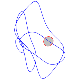
Figure 12. The shaded disk is the intersection $I_{0}^{+}\cap I_{1}^{+}$, which is contained in the interior of $I_{0}^{-}$.

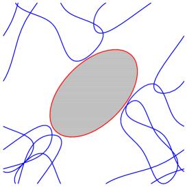
Figure 13. The shaded region is the ridge $I_{0}^{+}\cap I_{0}^{-}$.

Proposition 6.10.

The ridges $s_{0}^{+}\cap s_{-1}^{-}$ and $s_{0}^{+}\cap\widehat{s}_{-1}$ are topologically the union of two sectors.

Proof.

We parametrize the Giraud disk $I_{0}^{+}\cap I_{-1}^{-}$ by negative vectors of the form

$$V(z_{1},z_{2}) = \left(\overline{z_{1}}\mathbf{q}_{\infty}-B^{-1}(\mathbf{q}_{\infty})\right)\boxtimes\left(\overline{z_{2}}\mathbf{q}_{\infty}-A^{-1}B(\mathbf{q}_{\infty})\right)$$

$$= \left[\begin{array}[]{c}2z_{1}\\ -z_{1}+z_{2}-2\\ -2\\ \end{array}\right],$$

where $|z_{1}|=|z_{2}|=1$.

As in the above proposition, we can show that $I_{0}^{+}\cap I_{-1}^{-}$ lies outside the isometric spheres $I_{1}^{+},I_{-1}^{+},I_{0}^{-}$ and $\widehat{I}_{0}$. So we only need to consider the intersection of $I_{0}^{+}\cap I_{-1}^{-}$ and the isometric sphere $\widehat{I}_{-1}$. Their intersection can be described by the following equation

(6.3) $$|\langle V(z_{1},z_{2}),\mathbf{q}_{\infty}\rangle|=|\langle V(z_{1},z_{2}),A^{-1}BA^{-1}B(\mathbf{q}_{\infty})\rangle|.$$

Writing $z_{1}=e^{i\theta_{1}},z_{2}=e^{i\theta_{2}}$, Equation (6.3) is equivalent to

(6.4) $$-1-\cos(\theta_{1}-\theta_{2})+\cos(\theta_{1})+\cos(\theta_{2})=0.$$

The three solutions of Equation (6.4) are

$$\theta_{1}=0,\quad\theta_{2}=0,\quad\theta_{2}=\theta_{1}-\pi.$$

When $\theta_{2}=\theta_{1}-\pi$, we have

$$\langle V(z_{1},z_{2}),V(z_{1},z_{2})\rangle$$

$$= 6-2\sin(\theta_{1})\sin(\theta_{2})-2\cos(\theta_{1})\cos(\theta_{2})-4\cos(\theta_{1})-4\cos(\theta_{2})$$

$$= 8.$$

Therefore, the points $V(z_{1},z_{2})$ corresponding to the straight segment

$$\{\theta_{2}=\theta_{1}-\pi,\theta_{1}\in[-\pi,\pi]\}$$

lie entirely outside complex hyperbolic space.

We will see that the two crossed straight segments

$$\{\theta_{1}=0,\theta_{2}\in[-\arccos(1/3),\arccos(1/3)]\},$$

$$\{\theta_{2}=0,\theta_{1}\in[-\arccos(1/3),\arccos(1/3)]\}$$

decompose the Giraud disk $I_{0}^{+}\cap I_{-1}^{-}$ into four sectors with common vertices. Furthermore, one can check that one pair of the four sectors lie inside the isometric sphere $\widehat{I}_{-1}$. Therefore, the ridge $s_{0}^{+}\cap s_{-1}^{-}$ is the other pair of the four sectors. See Figure 15.

A similar analysis can be applied to the ridge $s_{0}^{+}\cap\widehat{s}_{-1}$. See Figure 15. ∎

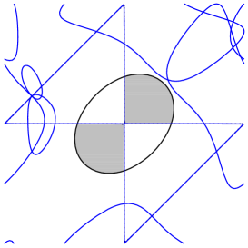
Figure 14. The ridge $s_{0}^{+}\cap s_{-1}^{-}$ on the Giraud disk $I_{0}^{+}\cap I_{-1}^{-}$ is the pair of shaded sectors.

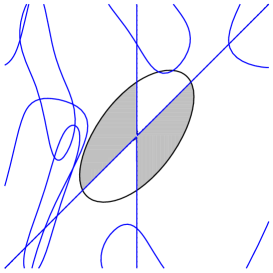
Figure 15. The ridge $s_{0}^{+}\cap\widehat{s}_{-1}$ on the Giraud disk $I_{0}^{+}\cap\widehat{I}_{-1}$ is the pair of shaded sectors.

Proposition 6.11.

The ridges $\widehat{s}_{0}\cap s_{0}^{-}$ and $\widehat{s}_{0}\cap s_{1}^{+}$ are topologically the union of two sectors.

One can also use the similar argument in Proposition 6.10 to show Proposition 6.11. We omit the details for the proof. Please refer to the Figures 17, 17.

Figure 16. The ridge $\widehat{s}_{0}\cap s_{0}^{-}$ on the Giraud disk $\widehat{I}_{0}\cap I_{0}^{-}$ is the pair of shaded sectors.

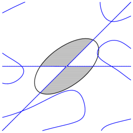
Figure 17. The ridge $\widehat{s}_{0}\cap s_{1}^{+}$ on the Giraud disk $\widehat{I}_{0}\cap I_{1}^{+}$ is the pair of shaded sectors.

Next, we describe the combinatorics of the sides.

Proposition 6.12.

1. The side $s_{k}^{+}$(resp. $s_{k}^{-}$) is a topological solid cylinder in $\mathbf{H}^{2}_{\mathbb{C}}\cup\partial\mathbf{H}^{2}_{\mathbb{C}}$. The intersection of $\partial s_{k}^{+}$(resp. $\partial s_{k}^{-}$) with $\mathbf{H}^{2}_{\mathbb{C}}$ is the disjoint union of two disks.

2. The side $\widehat{s}_{k}$ is a topological solid light cone in $\mathbf{H}^{2}_{\mathbb{C}}\cup\partial\mathbf{H}^{2}_{\mathbb{C}}$. The intersection of $\partial\widehat{s}_{k}$ with $\mathbf{H}^{2}_{\mathbb{C}}$ is a light cone.

Proof.

The side $s_{k}^{+}$ is contained in the isometric sphere $I_{k}^{+}$. It is bounded by the ridges $s_{k}^{+}\cap s_{k-1}^{-}$, $s_{k}^{+}\cap\widehat{s}_{k-1}$ and $s_{k}^{+}\cap s_{k}^{-}$. The ridges $s_{k}^{+}\cap s_{k-1}^{-}$ and $s_{k}^{+}\cap\widehat{s}_{k-1}$ are pair of sectors on the isometric sphere $I_{k}^{+}$. Furthermore, $I_{k}^{+}\cap I_{k}^{-}\cap\widehat{s}_{k-1}$ is the union of two crossed segments. Therefore, the union of the ridges $\widehat{s}_{k-1}\cap s_{k}^{+}$ and $s_{k-1}^{-}\cap s_{k}^{+}$ is a topological disc. Proposition 6.9 tell us that the smooth disc $s_{k}^{+}\cap s_{k}^{-}$ does not intersect with any other isometric sphere. This implies that $s_{k}^{+}$ is a topological solid cylinder. See Figure 18.

The side $\widehat{s}_{k}$ is bounded by two ridges $\widehat{s}_{k}\cap s_{k}^{-}$ and $\widehat{s}_{k}\cap s_{k+1}^{+}$. This two ridges are two pairs of sectors with common boundary which is the union of two crossed segments $\widehat{I}_{k}\cap I_{k}^{-}\cap I_{k+1}^{+}$. From the gluing process of two ridges along their boundaries, we see that $\widehat{s}_{k}$ is topological a solid light cone. See Figure 19. ∎

Figure 18. A schematic view of the side $s_{k}^{+}$.

Figure 19. A schematic view of the side $\widehat{s}_{k}$.

Applying a version of the Poincaré polyhedron theorem for coset decompositions, we show that $D_{\Gamma_{2}}$ will be the Ford domain for the group $\Gamma_{2}$ generated by $A$ and $B$.

Theorem 6.13.

$D_{\Gamma_{2}}$ is a fundamental domain for the cosets of $\langle A\rangle$ in $\Gamma_{2}$. Moreover, the group $\Gamma_{2}=\langle A,B\rangle$ is discrete and has the presentation

$$\langle A,B:B^{3}=(A^{-1}B)^{4}=id\rangle.$$

The side pairing maps are defined by:

$$A^{k}BA^{-k}: s_{k}^{+}\longrightarrow s_{k}^{-},$$

$$A^{k}(B^{-1}AB^{-1})A^{-k}: \widehat{s}_{k}\longrightarrow\widehat{s}_{k-1}.$$

Note that $D_{\Gamma_{2}}$ is invariant under a group $\langle A\rangle$ that is compatible with the side pairing maps.

By Corollary 6.5, the ridges are $s_{k}^{+}\cap s_{k-1}^{-}$, $s_{k}^{+}\cap\widehat{s}_{k-1}$, $s_{k}^{+}\cap s_{k}^{-}$, $s_{k}^{-}\cap\widehat{s}_{k}$ and $s_{k}^{-}\cap s_{k+1}^{+}$ for $k\in\mathbb{Z}$, and the sides and ridges are related as follows:

• The side $s_{k}^{+}$ is bounded by the ridges $s_{k}^{+}\cap s_{k-1}^{-}$, $s_{k}^{+}\cap\widehat{s}_{k-1}$ and $s_{k}^{+}\cap s_{k}^{-}$.

• The side $s_{k}^{-}$ is bounded by the ridges $s_{k}^{-}\cap\widehat{s}_{k}$, $s_{k}^{-}\cap s_{k+1}^{+}$ and $s_{k}^{+}\cap s_{k}^{-}$.

• The side $\widehat{s}_{k}$ is bounded by the ridges $\widehat{s}_{k}\cap s_{k}^{-}$ and $\widehat{s}_{k}\cap s_{k+1}^{+}$.

Proposition 6.14.

1. The side pairing $A^{k}BA^{-k}$ is a homeomorphism from $s_{k}^{+}$ to $s_{k}^{-}$. Moreover, it sends the ridges $s_{k}^{+}\cap s_{k-1}^{-}$, $s_{k}^{+}\cap\widehat{s}_{k-1}$ and $s_{k}^{+}\cap s_{k}^{-}$ to $s_{k}^{-}\cap\widehat{s}_{k}$, $s_{k}^{-}\cap s_{k+1}^{+}$ and $s_{k}^{+}\cap s_{k}^{-}$ respectively.

2. The side pairing $A^{k}(B^{-1}AB^{-1})A^{-k}$ is a homeomorphism from $\widehat{s}_{k}$ to $\widehat{s}_{k-1}$. Moreover, it sends the ridges $\widehat{s}_{k}\cap s_{k}^{-}$ and $\widehat{s}_{k}\cap s_{k+1}^{+}$ to $s_{k}^{+}\cap\widehat{s}_{k-1}$ and $s_{k-1}^{-}\cap\widehat{s}_{k-1}$ respectively.

Proof.

We only need to consider the case $k=0$. $s_{0}^{+}$ is contained in the isometric sphere $I_{0}^{+}$ and $s_{0}^{-}$ in the isometric sphere $I_{0}^{-}$. The ridge $s_{0}^{+}\cap s_{0}^{-}$ is the whole smooth disc $I_{0}^{-}\cap I_{0}^{+}$, which is defined by the triple equality

$$|\langle{\bf z},{\bf{q}_{\infty}}\rangle|=|\langle{\bf z},B^{-1}({\bf{q}_{\infty}})\rangle|=|\langle{\bf z},B({\bf{q}_{\infty}})\rangle|.$$

The elliptic element $B$ of order three sends this ridge to itself.

The ridge $s_{0}^{+}\cap s_{-1}^{-}$ is a pair of sectors contained in the disc $I_{0}^{+}\cap I_{-1}^{-}$, which is defined by the triple equality

$$|\langle{\bf z},{\bf{q}_{\infty}}\rangle|=|\langle{\bf z},B^{-1}({\bf{q}_{\infty}})\rangle|=|\langle{\bf z},A^{-1}B({\bf{q}_{\infty}})\rangle|.$$

$B$ maps $q_{\infty}$ to $B(q_{\infty})$, $B^{-1}(q_{\infty})$ to $q_{\infty}$ and $A^{-1}B(q_{\infty})$ to $BA^{-1}B(q_{\infty})$. That is, $B$ maps the disc $I_{0}^{+}\cap I_{-1}^{-}$ to the disc $I_{0}^{-1}\cap\widehat{I}_{0}$. Note that the other pair of sectors different from the ridge on the disc $I_{0}^{+}\cap I_{-1}^{-}$ lie in the interior of the isometric sphere $\widehat{I}_{-1}$, and the other pair of sectors different from the ridge on the disc $I_{0}^{-}\cap\widehat{I}_{0}$ lie in the interior of the isometric sphere $I_{1}^{+}$. One can check that the point $p^{\star}$ with homogeneous coordinates

$$p^{\star}=\left[\begin{array}[]{c}-\frac{\sqrt{2}}{2}-\frac{\sqrt{2}}{2}i\\ 1\\ 1\\ \end{array}\right]$$

is contained in the ridge $s_{0}^{+}\cap s_{-1}^{-}$. It is easily verified that $B(p^{\star})$ lies in the exterior of $I_{1}^{+}$. Thus $B(p^{\star})$ is contained in the ridge $s_{0}^{-1}\cap\widehat{s}_{0}$, lies in the exterior of the isometric sphere $I_{1}^{+}$. Hence $B$ maps the ridge $s_{0}^{+}\cap s_{-1}^{-}$ to the ridge $s_{0}^{-1}\cap\widehat{s}_{0}$. Similarly, the rest can be proved by using the same arguments. ∎

According to the side-paring maps, the ridge cycles are:

$$(s_{k}^{+}\cap s_{k-1}^{-},s_{k}^{+},s_{k-1}^{-})\xrightarrow{A^{k}BA^{-k}}(s_{k}^{-}\cap\widehat{s}_{k},\widehat{s}_{k},s_{k}^{-})\xrightarrow{A^{k}(B^{-1}AB^{-1})A^{-k}}$$

$$(\widehat{s}_{k-1}\cap s_{k}^{+},s_{k}^{+},\widehat{s}_{k-1})\xrightarrow{A^{k}BA^{-k}}(s_{k}^{-}\cap s_{k+1}^{+},s_{k+1}^{+},s_{k}^{-})\xrightarrow{A^{-1}}(s_{k}^{+}\cap s_{k-1}^{-},s_{k}^{+},s_{k-1}^{-}),$$

and

$$(s_{k}^{+}\cap s_{k}^{-},s_{k}^{+},s_{k}^{-})\xrightarrow{A^{k}BA^{-k}}(s_{k}^{-}\cap s_{k}^{+},s_{k}^{-},s_{k}^{+}).$$

Every ridge cycle is equivalent to one of the cycles listed above.

Note that $B^{-1}AB^{-1}=A^{-1}BA^{-1}BA^{-1}$. Thus the cycle transformations are

$$A^{-1}\cdot A^{k}BA^{-k}\cdot A^{k}(A^{-1}BA^{-1}BA^{-1})A^{-k}\cdot A^{k}BA^{-k}=A^{k}(A^{-1}B)^{4}A^{-k}=id.$$

and

$$(A^{k}BA^{-k})^{3}=A^{k}B^{3}A^{-k},$$

which are equal to the identity map, since we have $B^{3}=(A^{-1}B)^{4}=id$.

After Propositions 6.12 and 6.14, we now show

Local tessellation.

In our case, the intersection of each pair of two bisectors is a smooth disk. It follows from Proposition 2.6 that the ridges of $D_{\Gamma_{2}}$ are on precisely three isometric spheres, hence there are three copies of $D_{\Gamma_{2}}$ tiling its neighborhood. Therefore the ridge cycles satisfy the local tessellation conditions of the Poincaré polyhedron theorem.

Completeness

We must construct a system of consistent horoballs at the parabolic fixed points. First, we consider the side pairing maps on the parabolic fixed points in Proposition 6.14. We have

$$B : p_{AB}\longrightarrow B(p_{AB}),$$

$$AB^{-1}A^{-1} : p_{AB}\longrightarrow A(p_{AB}).$$

Up to powers of $A$, the cycles for the parabolic fixed points are the following

$$p_{AB}\xrightarrow{AB^{-1}A^{-1}}A(p_{AB})\xrightarrow{A^{-1}}p_{AB}.$$

That is, $p_{AB}$ is fixed by $B^{-1}A^{-1}$. The element $B^{-1}A^{-1}$ is parabolic and so preserves all horoballs at $p_{AB}$.

This ends the proof of Theorem 6.13.

7. Manifold at infinity of the complex hyperbolic triangle group $\Delta_{3,4,\infty;\infty}$

Based on the results in Section 6, in particular, the combinatorial structures of $I^{\pm}_{k}\cap\overline{\bf H}^{2}_{\mathbb{C}}$ and $\widehat{I}_{k}\cap\overline{\bf H}^{2}_{\mathbb{C}}$, we study the manifold at infinity of the even subgroup $\Gamma_{2}$ of the complex hyperbolic triangle group $\Delta_{3,4,\infty;\infty}$ in this section. We restate Theorem 1.6 as:

Theorem 7.1.

The manifold at infinity of $\Gamma_{2}$ is homeomorphic to the hyperbolic 3-manifold $m295$ in the Snappy Census.

The ideal boundary of $D_{\Gamma_{2}}$ is made up of the ideal boundaries of the sides $s_{k}^{\pm}$ and $\widehat{s}_{k}$. For convenience, when we speak of sides and ridges we implicitly mean their intersections with $\partial\mathbf{H}^{2}_{\mathbb{C}}$ in this section.

We first take four points in Heiserberg coordinates,

$$y = \left[\frac{4}{3}+\frac{\sqrt{2}}{3}i,0\right],$$

$$c = \left[\frac{4}{3}-\frac{\sqrt{2}}{3}i,0\right],$$

$$g = \left[\frac{2}{3}+\frac{\sqrt{2}}{3}i,-\frac{4\sqrt{2}}{3}\right],$$

$$r = \left[\frac{2}{3}-\frac{\sqrt{2}}{3}i,\frac{4\sqrt{2}}{3}\right].$$

In Figure 24, the point $y$ (resp. $g$, $c$, $r$) is indicated by a small yellow (resp. green, cyan, red) dot.

By simply calculation, we have

$$A(y)=B(g) = \left[-\frac{1}{6}+\frac{2\sqrt{2}-3\sqrt{7}}{6}i,\frac{2\sqrt{7}}{3}+\sqrt{2}\right],$$

$$A(g)=B(c) = \left[-\frac{5}{6}+\frac{2\sqrt{2}-3\sqrt{7}}{6}i,\frac{4\sqrt{7}-\sqrt{2}}{3}\right],$$

$$A(c)=B(r) = \left[-\frac{1}{6}-\frac{2\sqrt{2}+3\sqrt{7}}{6}i,\frac{2\sqrt{7}}{3}-\sqrt{2}\right],$$

$$A(r)=B(y) = \left[-\frac{5}{6}-\frac{2\sqrt{2}+3\sqrt{7}}{6}i,\frac{4\sqrt{7}+\sqrt{2}}{3}\right].$$

Figure 20. The ideal side $s_{0}^{+}$ is the region exterior to the three Jordan closed curves $I_{0}^{+}\cap I_{-1}^{-}$, $I_{0}^{+}\cap\widehat{I}_{-1}$ and $I_{0}^{+}\cap I_{1}^{-}$ on the spinal sphere of $B$. These Jordan curves are drawn with geographical coordinates introduced in [23].

Figure 21. The side $s_{0}^{+}$ on the blue spinal sphere $I_{0}^{+}$ is topologically an annulus.

Figure 22. The side $\widehat{s}_{0}$ on the blue spinal sphere with two disjoint connect components.

Now we study the combinatorial properties of the sides. See Figures 20, 22, 22 and 24.

Proposition 7.2.

• The interior of the side $s_{0}^{+}$ is an annulus. One boundary component of it is the Jordan curve $s_{0}^{+}\cap s_{0}^{-}$ and the other boundary component is a quadrilateral with vertices $y,g,c,r$.

• The interior of the side $\widehat{s}_{0}$ has two disjoint connected components. Each component is a bigon. One bigon with vertices $A(y),A(g)$ and the other bigon with vertices $A(c),A(r)$.

Proof.

(1). The traces of the Giraud disks $I_{0}\cap I_{-1}^{-}$ and $I_{0}\cap\widehat{I}_{-1}$ on the spinal sphere $I_{0}$ are two closed Jordan curves. By simple calculation, we see that there are four intersection points (labeled by $y$, $g$, $c$ and $r$) of this two closed curves. From the structure of the ridges, we known that the trace of the ridge $s_{0}\cap s_{-1}^{-}$ (resp. $s_{0}\cap\widehat{s}_{-1}$) is a union of two Jordan arcs $[y,g]$ and $[c,r]$ (resp. $[g,c]$ and $[r,y]$). The trace of the ridge $s_{0}\cap s_{-1}$ on the spinal sphere $I_{0}$ is also a closed Jordan curve. Note that $I_{-1}$ does not intersect with $I_{-1}^{-}$ and $\widehat{I}_{-1}$. This completes the proof of the first part of Proposition 7.2. See Figure 23.

(2). From the structure of the side $\widehat{s}_{0}$, the side $\widehat{s}_{0}$ in the ideal boundary is the union of two disjoint discs, which are bounded by the ideal boundary of the ridges $\widehat{s}_{0}\cap s_{0}^{-}$ and $\widehat{s}_{0}\cap s_{1}^{+}$. By calculation, we find the intersection of $\widehat{I}_{0}\cap I_{0}^{-}\cap I_{1}^{+}$ with the ideal boundary are the four points $A(y),A(g),A(c),A(r)$. We will determine that one component on the ideal side $\widehat{s}_{0}$ with vertices $A(y),A(g)$ and the other component with vertices $A(c),A(r)$. We only prove the first case. We choose a point $p^{\diamond}$ on the spinal sphere $\widehat{I}_{0}$ with Heisenberg coordinates

$$\left[-\frac{1}{2}+(1-\frac{\sqrt{7}}{2})i,1+\sqrt{7}\right]$$

such that $p^{\diamond}$ lies outside the spinal spheres $I_{0}^{-}$ and $I_{1}^{+}$. One can also check that the two straight line segments $[A(y),p^{\diamond}]$ and $[A(g),p^{\diamond}]$ also lie outside the spinal spheres $I_{0}^{-}$ and $I_{1}^{+}$ other than the two end points $A(y)$ and $A(g)$. Therefore, the points $A(y)$, $A(g)$ must be the vertices of one bigon and the points $A(c)$, $A(r)$ must be the vertices of the another bigon.

∎

7.1. A global combinatorial model of the boundary at infinity of the Ford domain of $\Delta_{3,4,\infty;\infty}$

We have shown in Section 6 the ideal boundary of the Ford domain of $\Delta_{3,4,\infty;\infty}$ consists of $A$-translates of isometric spheres of $\{B,B^{-1},B^{-1}AB^{-1},BA^{-1}B\}$. We gave the detailed local information on these spinal spheres previously, and we now study the global topology of the region which is outside of all spinal spheres, which is $D_{\Gamma_{2}}\cap\partial\mathbf{H}^{2}_{\mathbb{C}}$. From these information we can identify the topology of the manifold at infinity.

Figure 23 is a realistic view of the ideal boundary of the Ford domain of $\Delta_{3,4,\infty;\infty}$ with center $q_{\infty}$. This figure is just for motivation, and we need to show the figure is correct. We hope the figure is explicit enough such that the reader can see the “holes” in Figures 23. For example, one of them is the white region enclosed by the spinal spheres $I_{0}^{+}$, $I_{0}^{-}$, $I_{-1}^{-}$, $I_{-1}^{+}$. The ideal boundary of Ford domain is just the intersection of the exteriors of all the spinal spheres. Moreover, since the realistic view in Figure 23 is difficult to understand, we show a combinatorial model of it in Figure 24. Our computations later will show the combinatorial model coincides with Figure 23.

Figure 23. Realistic view of the ideal boundary of the Ford domain of $\Delta_{3,4,\infty;\infty}$, which is the region outside all of the spheres.

Figure 24. A combinatorial picture of the ideal boundary of the Ford domain of $\Delta_{3,4,\infty;\infty}$, which is out side of the singular surface $\Sigma$.

It seems to the authors that it is very difficult to write down explicitly the definition equations for the intersections of the spinal spheres of $\{B,A^{-1}B^{-1}A\}$, $\{B,A^{-1}B^{-1}AB^{-1}A\}$ and $\{A^{-1}B^{-1}A,A^{-1}B^{-1}AB^{-1}A\}$ in the Heisenberg group, even though we have proved each of them is a circle, and the intersection of any of them with ideal boundary of the Ford domain is one or two arcs. In this section, we first describe a global combinatorial object. We then use geometric arguments to show that it is combinatorially equivalent to the ideal boundary of the Ford domain of $\Delta_{3,4,\infty;\infty}$. Last, we describe the topology of the manifold at infinity of $\Delta_{3,4,\infty;\infty}$ from the combinatorial model. In particular, we will show that the ideal boundary of the Ford domain of $\Delta_{3,4,\infty;\infty}$ is an infinite genus $A$-invariant handlebody.

We first take $C^{*}$ to be the plane

(7.1) $$\left\{\left[r-\frac{1}{2},r-\frac{\sqrt{7}}{2},s\right]\,\Big{|}\,r,s\in\mathbb{R}\right\}$$

in the Heisenberg group. See Figure 25 for part of this plane, which is the red plane in Figure 25.

Figure 25. Realistic view of the $A$-invariant plane $C^{*}$ for the Ford domain of $\Delta_{3,4,\infty;\infty}$.

We now consider the intersections of $C^{*}$ with the spinal spheres of $B$, $B^{-1}$, $ABA^{-1}$, and $AB^{-1}A^{-1}$:

$I_{0}^{+}\cap C^{*}$ is the circle in $C^{*}$ with equation

(7.2) $$\left(\left(r-1/2\right)^{2}+\left(r-\sqrt{7}/2\right)^{2}\right)^{2}+s^{2}=4;$$

$I_{0}^{-}\cap C^{*}$ is the circle in $C^{*}$ with equation

(7.3) $$\left(\left(r-1\right)^{2}+r^{2}\right)^{2}+\left(s+r-\sqrt{7}+\sqrt{7}r\right)^{2}=4;$$

$I_{1}^{+}\cap C^{*}$ is the circle in $C^{*}$ with equation

(7.4) $$\left(\left(r+1\right)^{2}+r^{2}\right)^{2}+\left(s-\sqrt{7}-3r+\sqrt{7}r\right)^{2}=4;$$

$I_{1}^{-}\cap C^{*}$ is the circle in $C^{*}$ with equation

(7.5) $$\left(\left(r+1/2\right)^{2}+\left(r+\sqrt{7}/2\right)^{2}\right)^{2}+\left(s-2r+2\sqrt{7}r\right)^{2}=4.$$

Now $C^{*}$ passes through $[-\frac{1}{2},-\sqrt{7}/2,0]$, which is the tangent point of the spinal spheres $I_{0}^{+}$ and $I_{1}^{-}$ in the Heisenberg group, and it corresponds to the point $p_{AB}$ in Section 6, which is also the point $r=s=0$ in Figure 26.

With the definition equations above, it can be showed rigorously that the circles $I_{0}^{+}\cap C^{*}$ and $I_{0}^{-}\cap C^{*}$ intersect in four points in $C^{*}$, we take one of them with coordinates $r_{1}=0.038807$ and $s_{1}=0.7312373192$ numerically, and in fact $r_{1}$ is one root of

(7.6) $$\begin{split}1-14r-6\sqrt{7}r+70r^{2}+16\sqrt{7}r^{2}-94r^{3}-30\sqrt{7}r^{3}\\ +88r^{4}+20\sqrt{7}r^{4}-36r^{5}-12\sqrt{7}r^{5}+16r^{6}=0.\end{split}$$

Equation (7.6) has a pair of complex roots $0.693921\pm 1.3301i$ and four real roots $0.0388075$, $0.713275$, $0.741563$ and $1.35283$ numerically.

From the equations above, we can see that $I_{0}^{-}\cap C^{*}$ and $I_{1}^{-}\cap C^{*}$ intersect in four points in $C^{*}$. We take one of them, say $r=0$ and $s=\sqrt{7}-\sqrt{3}$, which is the upper vertex of the red disk in Figure 26.

The circles $I_{1}^{+}\cap C^{*}$ and $I_{1}^{-}\cap C^{*}$ intersect in four points in $C^{*}$, we take one of them with coordinates $r_{2}=-0.038807$ and $s_{2}=0.858972$ numerically, and in fact $r_{2}$ is one root of

(7.7) $$\begin{split}1+\sqrt{7}+56r+20\sqrt{7}r+182r^{2}+86\sqrt{7}r^{2}+304r^{3}+124\sqrt{7}r^{3}\\ +228r^{4}+108\sqrt{7}r^{4}+120r^{5}+48\sqrt{7}r^{5}+16r^{6}+16\sqrt{7}r^{6}=0.\end{split}$$

Equation (7.7) has a pair of complex roots $0.693921\pm 1.3301i$ and four real roots $-0.0388075$, $-1.35283$, $-0.741563$ and $-0.713275$ numerically.

Figure 26. The small red colored disk $C$ in the plane $C^{*}$ which is co-bounded by four arcs lying in $C^{*}\cap I_{0}^{-}$, $C^{*}\cap I_{0}^{+}$, $C^{*}\cap I_{1}^{+}$ and $C^{*}\cap I_{1}^{-}$ respectively.

We take $L_{0}$ be the arc in $I_{0}^{+}\cap C^{*}$ with $r\in[0,r_{1}]$ and $s\in[0,s_{1}]$, which is the intersection of the red circle and the red disk in Figure 26. Take $L_{1}$ to be the arc in $I_{0}^{-}\cap C^{*}$ with $r\in[0,r_{1}]$ and $s\in[s_{1},\sqrt{7}-\sqrt{3}]$, which is the steelblue boundary arc of the red disk in Figure 26. Note that $s$ decreases as function of $r$ in $L_{1}$. Take $L_{2}$ to be the arc in $I_{1}^{+}\cap C^{*}$ with $r\in[r_{2},0]$ and $s\in[s_{2},\sqrt{7}-\sqrt{3}]$, which is the green boundary arc of the red disk in Figure 26, $s$ also decreases as function of $r$ in $L_{2}$. Take $L_{3}$ to be the arc in $I_{1}^{-}\cap C^{*}$ with $r\in[r_{2},0]$ and $s\in[0,s_{2}]$, which is the black boundary arc of the red disk in Figure 26.

Lemma 7.3.

The union of four arcs $L_{0}\cup L_{1}\cup L_{2}\cup L_{3}$ is a simple closed curve in $C^{*}$.

Proof.

From the above chosen parameters of these arcs, it is easy to see that $L_{i}$ only intersects with $L_{i-1}$ and $L_{i+1}$ in its two end vertices, and $L_{i}$ does not intersect $L_{i+2}$, for $i=0,1,2,3\mod 4$. So $L_{0}\cup L_{1}\cup L_{2}\cup L_{3}$ is a simple closed curve in $C^{*}$. ∎

We take $C$ be the disk in the plane $C^{*}$ with boundary $L_{0}\cup L_{1}\cup L_{2}\cup L_{3}$.

Lemma 7.4.

The disk $C$ has the following properties:

(1). The boundary of $C$ is a union of four arcs, in the spinal spheres of $B$, $B^{-1}$, $ABA^{-1}$ and $AB^{-1}A^{-1}$ cyclically.

(2). The interior of the disk $C$ is disjoint from all the spinal spheres of $A$-translations of $B$, $B^{-1}$ and $B^{-1}AB^{-1}$.

(3). The disk $C$ and any translation $A^{k}(C)$ for $k\neq 0$ are disjoint.

Proof.

We have proved (1) of Lemma 7.4 above.

For (2) of Lemma 7.4, from the vertical projections of the disk $C$, and the spinal spheres $I_{k}^{\pm}$ and $\widehat{I}_{k}$ for $k\in\mathbb{Z}$, to the plane $\mathbb{C}$, we can easy see that $C$ does not intersect the spinal spheres $I_{k}^{\pm}$ and $\widehat{I}_{k}$ except $I_{0}^{+}$, $I_{0}^{-}$, $I_{1}^{+}$, $I_{1}^{-}$ and $\widehat{I}_{0}$. See Figure 29 for the vertical projections of them.

The intersection $\widehat{I}_{0}\cap C^{*}$ is a circle

(7.8) $$(2r^{2})^{2}+(s-\sqrt{7}-r+\sqrt{7}r)^{2}=1,$$

in the $rs$-plane $C^{*}$. Note that $\sqrt{7}-\sqrt{3}$ is the largest one of $s$-coordinate of the disk $C$, but take $s=\sqrt{7}-\sqrt{3}$ in Equation (7.8), there is no real solution of $r$ (numerically, there are four solutions $r=-0.555156\pm 0.0702174i$ and $0.555156\pm 1.13516i$). Take a sample point on $\widehat{I}_{0}\cap C^{*}$, for example $r=0$, $s=\sqrt{7}-1$. Note that $s=\sqrt{7}-1>s=\sqrt{7}-\sqrt{3}$, this means that the $s$-coordinate of any point in the circle $\widehat{I}_{0}\cap C^{*}$ is larger than $\sqrt{7}-\sqrt{3}$. So the disk $C$ does not intersect with $\widehat{I}_{0}$.

For (3) of Lemma 7.4, note that $A^{k}(C)$ is a subdisk of the square $r\in[-0.038,-0.038]$ numerically and $s\in[0,\sqrt{7}-\sqrt{3}]$ in the plane $A^{k}(C^{*})$

(7.9) $$\left[r-\frac{1+3k}{2},r-\frac{\sqrt{7}(k+1)}{2},s+3kr+k\sqrt{7}-kr\sqrt{7}\right],$$

with $r,s$ reals in Heisenberg coordinates. Then it is easy to see $C$ and $A^{k}(C)$ are disjoint disks for $k\neq 0$ in the Heisenberg group.

∎

We then take $E^{*}$ to be the plane

(7.10) $$\left[r+\frac{1}{4},-2r-\frac{\sqrt{7}}{4},r+s-\frac{\sqrt{7}}{2}\right]$$

with $r$ and $s$ reals in Heisenberg coordinates. See Figure 27 for part of this plane, $E^{*}$ is one of the blue planes in Figure 27.

Figure 27. The plane $E^{*}$ intersects only the spinal spheres of $B$ and $B^{-1}$ and the plane $A(E^{*})$ intersects only the spinal spheres of $ABA^{-1}$ and $AB^{-1}A^{-1}$.

We consider the intersections of $I_{0}^{+}$ and $I_{0}^{-}$ with $E^{*}$: $I_{0}^{+}\cap E^{*}$ has the definition equation

(7.11) $$\left(\left(r+\frac{1}{4}\right)^{2}+\left(2r+\frac{\sqrt{7}}{4}\right)^{2}\right)^{2}+\left(r+s-\frac{\sqrt{7}}{2}\right)^{2}=4$$

with $r$ and $s$ reals. It is easy to see Equation (7.11) gives us a closed curve in the $rs$-plane $E^{*}$.

Lemma 7.5.

$I_{0}^{+}\cap E^{*}$ is a simple closed curve in $E^{*}$.

Proof.

For the Equation (7.11), we can solve $s$ in terms of $r$ as

$$s=\frac{1}{4}\sqrt{7}-r\pm\frac{1}{2}\sqrt{-40r^{3}\sqrt{7}-100r^{4}-4r^{2}\sqrt{7}-20r^{3}+15-4r\sqrt{7}-49r^{2}-2r}.$$

For one real $r$, there are at most two reals $s$ satisfying Equation (7.11), and there is exactly one real $s$ satisfying Equation (7.11) when

(7.12) $$-40r^{3}\sqrt{7}-100r^{4}-4r^{2}\sqrt{7}-20r^{3}+15-4r\sqrt{7}-49r^{2}-2r=0.$$

Equation (7.12) has a pair of complex roots, and a pair of real toots

$$r=-\frac{1}{20}-\frac{\sqrt{7}}{10}\pm\frac{\sqrt{149+4\sqrt{7}}}{20},$$

which are the maximum and the minimum of $r$ satisfies Equation (7.11). So the curve $I_{0}^{+}\cap E^{*}$ is a simple closed curve, that is, there is no self-intersection. ∎

Similarly, we can prove $I_{0}^{-}\cap E^{*}$ is a simple closed curve in the plane $E^{*}$ with definition equation

(7.13) $$\left(\left(r-1/4\right)^{2}+\left(-2r+\sqrt{7}/4\right)^{2}\right)^{2}+\left(s-r+\sqrt{7}r-\sqrt{7}/2\right)^{2}=4$$

with $r$ and $s$ reals.

Now we can solve algebraically that the triple intersection $I_{0}^{+}\cap I_{0}^{-}\cap E^{*}$ are two points with $r=0$ and $s=\pm\sqrt{15}/2+\sqrt{7}/2$ in the $rs$-plane $E^{*}$. They are the points $\left[1/4,-\sqrt{7}/4,\pm\sqrt{15}/2\right]$ in the Heisenberg group. In other words, simple closed curves $I_{0}^{+}\cap E^{*}$ and $I_{0}^{-}\cap E^{*}$ intersect in exactly two points. Each of $I_{0}^{+}\cap E^{*}$ and $I_{0}^{-}\cap E^{*}$ bounds a closed disk in $E^{*}$, now the union of them is a bigger disk in $E^{*}$, we denote it by $E$. See Figure 28.

Figure 28. The intersection of the plane $E^{*}$ with $I_{0}^{+}$, $I_{0}^{-}$, $\widehat{I}_{-1}$ and $\widehat{I}_{0}$. The disk $E$ lies in the plane $E^{*}$ is co-bounded by two arcs lying in two Jordan curves $I_{0}^{+}\cap E^{*}$ and $I_{0}^{-}\cap E^{*}$. $E$ is the disk which is the complement of the outer green region. The tangent point of $\widehat{I}_{-1}\cap E^{*}$ and $\widehat{I}_{0}\cap E^{*}$ is the point $[\frac{1}{4},-\frac{\sqrt{7}}{4},-\frac{\sqrt{7}}{2}]$ in the Heisenberg group, which is the triple intersection $\widehat{I}_{-1}\cap\widehat{I}_{0}\cap E^{*}$.

Lemma 7.6.

The plane $E^{*}$ and disk $E$ have the following properties:

(1). The boundary of $E$ is a union of two arcs: one in the spinal sphere of $B$ and the other in the spinal sphere of $B^{-1}$.

(2). The interior of the holed plane $E^{*}-E$ is disjoint from all the spinal spheres of $A$-translations of $B$, $B^{-1}$ and $B^{-1}AB^{-1}$.

(3). The plane $E^{*}$ and any translation $A^{k}(E^{*})$ for $k\neq 0$ are disjoint.

Proof.

We have proved (1) of Lemma 7.6 above.

For (2) of Lemma 7.6, the vertical projection of the plane $E^{*}$ to $\mathbb{C}$-plane is a line

(7.14) $$\left\{r+\frac{1}{4}+\left(-2r-\sqrt{7}/4\right)i\in\mathbb{C}\right\}$$

with $r$ reals. From the equations of $I^{+}_{k}$, $I^{-}_{k}$ and $\widehat{I_{k}}$, we can get the vertical projections of them to the $\mathbb{C}$-plane. It is easy to see that the vertical projection of $E^{*}$ only intersects with the vertical projections of $I^{+}_{0}$, $I^{-}_{0}$, $\widehat{I}_{0}$ and $\widehat{I}_{-1}$ from the equations of their vertical projections on the $\mathbb{C}$-plane.

We can write down the equation of the circle $\widehat{I}_{0}\cap E^{*}$ in the $rs$-plane $E^{*}$, which is a circle

(7.15) $$\left(\left(r+\frac{3}{4}\right)^{2}+\left(2r-\frac{\sqrt{7}}{4}\right)^{2}\right)^{2}+\left(s+3r-\sqrt{7}+\sqrt{7}r\right)^{2}=1.$$

Then $s$ is solved as function of $r$,

$$-\sqrt{7}r+\sqrt{7}-3r\pm\frac{\sqrt{-12r+8\sqrt{7}r-77r^{2}+12\sqrt{7}r^{2}-60r^{3}+40r^{3}\sqrt{7}-100r^{4}}}{2}.$$

We can also write down the equation of the circle $\widehat{I}_{-1}\cap E^{*}$ in the $rs$-plane $E^{*}$, which is a circle

(7.16) $$\left(\left(r-\frac{3}{4}\right)^{2}+\left(2r+\frac{\sqrt{7}}{4}\right)^{2}\right)^{2}+\left(s-3r-\sqrt{7}\right)^{2}=1,$$

and we can solve $s$ as function of $r$

(7.17) $$\sqrt{7}+3r\pm\frac{\sqrt{-40r^{3}\sqrt{7}-100r^{4}+12\sqrt{7}r^{2}+60r^{3}-8\sqrt{7}r-77r^{2}+12r}}{2}.$$

See Figure 28 for the circles $\widehat{I}_{0}\cap E^{*}$ and $\widehat{I}_{-1}\cap E^{*}$ in the $rs$-plane $E^{*}$. By solving the equations of them, it is easy to see that there is no triple intersection of $I_{0}^{+}$, $\widehat{I}_{0}$ and $E^{*}$, then the two circles $\widehat{I}_{0}\cap E^{*}$ and $I_{0}^{+}\cap E^{*}$ are disjoint in the place $E^{*}$. Take a sample point on $\widehat{I}_{0}\cap E^{*}$, for example, take $r=s=0$, we can see $\widehat{I}_{0}\cap E^{*}$ lies in the disk bounded by $I_{0}^{+}\cap E^{*}$ in the place $E^{*}$. Similarly, we can see $\widehat{I}_{0}\cap E^{*}$ lies in the disk bounded by $I_{0}^{-}\cap E^{*}$ in the place $E^{*}$; $\widehat{I}_{-1}\cap E^{*}$ lies in the disk bounded by $I_{0}^{+}\cap E^{*}$ in the place $E^{*}$; $\widehat{I}_{-1}\cap E^{*}$ lies in the disk bounded by $I_{0}^{-}\cap E^{*}$ in the place $E^{*}$. So these two circles lie in the disk $E$.

For (3) of Lemma 7.6, by the equation of $E^{*}$ and the action of $A$, we get that the vertical projection of the plane $A^{k}(E^{*})$ to $\mathbb{C}$-plane is the line,

(7.18) $$\left\{r+\frac{1}{4}-\frac{3k}{2}+\left(-2r-\frac{\sqrt{7}(1+2k)}{4}\right)i\in\mathbb{C}\right\}$$

with $r$ real, so the vertical projections of $E^{*}$ and $A^{k}(E^{*})$ for $k\neq 0$ are disjoint parallel lines, then $E^{*}$ and $A^{k}(E^{*})$ are disjoint in the Heisenberg group for $k\neq 0$. ∎

Figure 29. The vertical projections of the planes $E^{*}$, $C^{*}$ and the spinal spheres of $I_{k}^{-}$, $I_{k}^{+}$ and $\widehat{I}_{k}$ for $k=-1,0,1$. The (very) short thick red arc is the vertical projection of the disk $C$.

In Figure 30, we give the abstract pictures of annuli of the intersections of $I_{0}^{+}$ and $I_{0}^{-}$ with the ideal boundary of the Ford domain of $\Delta_{3,4,\infty;\infty}$. The abstract pictures of annuli of the intersections of $I_{k}^{+}$ and $I_{k}^{-}$ with the ideal boundary of the Ford domain of $\Delta_{3,4,\infty;\infty}$ are similar by the $A$-action.

Figure 30. The punctured annuli of the intersections of $I_{0}^{+}$ and $I_{0}^{-}$ with the ideal boundary of the Ford domain of $\Delta_{3,4,\infty;\infty}$. The left-side is the annulus for $I_{0}^{+}$, the green arc is the intersection of this annulus and the disk $E$; the pink arc is the intersection of this annulus and the disk $C$; the three arcs labeled by $B^{-1}$ mean these arcs are glued to annulus for $I_{0}^{-}$; the two arcs labeled by $A^{-1}B^{-1}A$ mean these arcs are glued to annulus for $I_{-1}^{-}$; the two arcs labeled by $A^{-1}B^{-1}AB^{-1}A$ mean these arcs are glued to bigons for $\widehat{I}_{-1}$. The right-side is the annulus for $I_{0}^{+}$, the labels obey the similar law as the left-side.

Take a singular surface

$$\Sigma=\bigcup_{k\in\mathbb{Z}}((\hat{s}_{k}\cup s_{k}^{\pm})\cap\partial\mathbf{H}^{2}_{\mathbb{C}})$$

in the Heisenberg group. See Figure 24 for an abstract picture of this surface. $\Sigma$ is an annulus with $A$-action and which is tangent to itself at infinite many points.

From the $A$-action on the plane $E^{*}$ we get a plane $A(E^{*})$

(7.19) $$\left[r-\frac{5}{4},-2r-\frac{3\sqrt{7}}{4},-5r+s+\frac{(1-2r)\sqrt{7}}{2}\right]$$

with $r$ and $s$ reals in the Heisenberg group. In particular, $E^{*}$ and $A(E^{*})$ are parallel planes in the Heisenberg group. One component of $(\partial{\bf H}^{2}_{\mathbb{C}}\backslash\{q_{\infty}\})\backslash(E^{*}\cup A(E^{*}))$ contains the disk $C$, we denote the closure of this component by $U$, $U$ is homeomorphic $E^{*}\times[0,1]$. We denote by $H$ the closure of complement of all the 3-balls bounded $\hat{s}_{k}$ and $s_{k}^{\pm}$ in $U$. Note that

$$\partial_{\infty}D_{\Gamma_{2}}=\cup^{\infty}_{k=-\infty}A^{k}(H).$$

We will show $\partial_{\infty}D_{\Gamma_{2}}$ is an infinite genus handlebody in the Heisenberg group.

Figure 31. The eleven pieces of a 2-sphere $S$ for the Ford domain of $\Delta_{3,4,\infty;\infty}$.

We consider a surface $S$ which is a union of eleven pieces, see Figure 31:

• the top two in Figure 31 are the remaining disks of $I_{0}^{+}$ and $I_{1}^{-}$, we denote them by $F(B)$ and $F(AB^{-1}A^{-1})$ respectively, that is, $F(B)=(I_{0}^{+}\cap H)\backslash C$ and $F(AB^{-1}A^{-1})=(I_{1}^{-}\cap H)\backslash C$. Each of $F(B)$ and $F(AB^{-1}A^{-1})$ is a hexagon. The boundary arcs of $F(B)$ are labeled by $B^{-1}$, $E$, $B^{-1}$, $C(-)$, $F$ and $C(+)$ cyclically, this means that $F(B)$ is glued to the disks $F(B^{-1})$, $E$, $F(B^{-1})$, $C(-)$, $F$ and $C(+)$ in Figure 31 along these arcs. Similarly $F(AB^{-1}A^{-1})$ is glued to the disks $F(ABA^{-1})$, $A(E)$, $F(ABA^{-1})$, $C(-)$, $F$ and $C(+)$ in Figure 31 along its boundary.

• the two disks in the second row of Figure 31 are the remaining disks of $I_{0}^{-}$ and $I_{1}^{+}$, we denote them by $F(B^{-1})$ and $F(ABA^{-1})$ respectively, that is, $F(B^{-1})=(I_{0}^{-}\cap H)\backslash C$ and $F(ABA^{-1})=(I_{1}^{+}\cap H)\backslash C$. Each of $F(B^{-1})$ and $F(ABA^{-1})$ is a decagon. $F(B^{-1})$ is glued to the disks $E$, $F(B)$, $C(+)$, $F(ABA^{-1})$, $F(B^{-1}AB^{-1})$, $F(AB^{-1}A^{-1})$, $F(B^{-1}AB^{-1})$, $F(ABA^{-1})$, $C(-)$ and $F(B)$ in Figure 31 along its boundary. Similarly $F(ABA^{-1})$ is glued to ten disks in Figure 31.

• The disks $C(+)$ and $C(-)$ in the third row of Figure 31 are two copies of the disk $C$ but with a vertex link of the vertex $p_{AB}$ deleted, so each of $C(+)$ and $C(-)$ is a pentagon. The disk $F$ in the third row of Figure 31 is a square, which is glued to $C(+)$, $C(-)$, $F(B)$ and $F(AB^{-1}A^{-1})$.

• The disks $E$ and $A(E)$ in the fourth row of Figure 31 are glued to $F(B)$, $F(B^{-1})$ and $F(ABA^{-1})$, $F(AB^{-1}A^{-1})$ respectively. The disks $F(B^{-1}AB^{-1},1)$ and $F(B^{-1}AB^{-1},2)$ in the fourth row of Figure 31 are the remaining disks of $\widehat{I}_{0}^{-}$, that is, $F(B^{-1}AB^{-1},1)\cup F(B^{-1}AB^{-1},2)=\widehat{I}_{0}^{-}\cap H$.

Figure 32. Gluing all of eleven pieces in Figure 31, we get a 2-sphere.

We now glue all together the eleven pieces to a surface $S$.

Lemma 7.7.

The surface $S$ above is a 2-sphere.

Proof.

Even through we can show this lemma by the calculation of the Euler characteristic of $S$, but we prefer to show it via a picture. Figure 32 is a 2-disk, we glue the two biggest (and outer) arcs which is one arc of the boundary of the disk labeled by $F(B^{-1})$ and $F(ABA^{-1})$ respectively, we get a 2-sphere. Now the gluing patterns of the eleven pieces are the same as the gluing pattern of Figure 31, so $S$ above is a two sphere. ∎

Note that the sphere $S$ is the boundary of a neighborhood of $(U-H)\cup C$ in the Heisenberg group. In particular, $S$ bounds a 3-ball containing $(U-H)\cup C$ in the Heisenberg group. Note that $S$ and $A(S)$ intersect in the disk $A(E)$, so the two 3-balls bounded by $S$ and $A(S)$ intersect in the disk $A(E)$. Then a neighborhood of

$$\cup^{\infty}_{k=-\infty}A^{k}((U-H)\cup C)$$

in the Heisenberg group is homeomorphic to $\mathbb{D}^{2}\times(-\infty,\infty)$. By Proposition 7.8 bellow, this $\mathbb{D}^{2}\times(-\infty,\infty)$ with $A$-action is unknotted in the Heisenberg group. So the complement of a neighborhood of $\cup^{\infty}_{k=-\infty}A^{k}((U-H)\cup C)$ in the Heisenberg space is homeomorphic to $(\mathbb{R}^{2}\backslash\mathbb{D}^{2})\times(-\infty,\infty)$, which is a genus one handlebody. Then $\partial_{\infty}D_{\Gamma_{2}}$ is an infinite genus handlebody with $A$-action, such that if we cut $\partial_{\infty}D_{\Gamma}$ along the infinite many disjoint disks $\{A^{k}(C)\}^{\infty}_{k=-\infty}$, we get $(\mathbb{R}^{2}\backslash\mathbb{D}^{2})\times(-\infty,\infty)$.

Proposition 7.8.

The affine line in Heisenberg coordinates

$$L=\left\{\left[-\frac{3}{2}x+\frac{5}{4},-\frac{\sqrt{7}}{2}x+\frac{\sqrt{7}}{5},\frac{27\sqrt{7}}{20}x-\frac{3\sqrt{7}}{4}\right]\in\partial\mathbf{H}^{2}_{\mathbb{C}};x\in\mathbb{R}\right\}$$

is preserved by the map $A$. Moreover $L$ is contained in the complement of $D_{\Gamma_{2}}$.

Proof.

We denote by

$$L_{x}=\left[-\frac{3}{2}x+\frac{5}{4},-\frac{\sqrt{7}}{2}x+\frac{\sqrt{7}}{5},\frac{27\sqrt{7}}{20}x-\frac{3\sqrt{7}}{4}\right]$$

a point in $L$. The parabolic map $A$ acts on $L$ as:

$$A:L_{x}\rightarrow L_{x+1}.$$

So $A$ acts on $L$ as a translation through 1. We claim that the segment on $L$ with parameter $x\in[0,1]$ is contained in $I_{0}^{+}\cup I_{-1}^{-}$. It is easy to check that the segment on $L$ with parameter $x\in[1/3,1]$ is contained in the interior of the spinal sphere $I_{0}^{+}$ and the segment on $L$ with parameter $x\in[0,1/3]$ in the interior of the spinal sphere $I_{-1}^{-}$. Therefore, the line $L$ is in the complement of $D_{\Gamma_{2}}$. ∎

Now we have

Lemma 7.9.

$\partial_{\infty}D_{\Gamma_{2}}$ is an infinite genus handlebody with $A$-action, such that the 3-manifold $\partial_{\infty}D_{\Gamma_{2}}/\Gamma_{2}$ at infinity of $\Gamma_{2}$ is obtained from $\partial_{\infty}D_{\Gamma_{2}}$ by side-pairings on $I_{k}^{+}\cap\partial_{\infty}D_{\Gamma_{2}}$, $I_{k}^{-}\cap\partial_{\infty}D_{\Gamma_{2}}$ and $\widehat{I}_{k}^{+}\cap\partial_{\infty}D_{\Gamma_{2}}$ for all $k\in\mathbb{Z}$.

In Figure 24, we give a combinatorial model of $\partial_{\infty}D_{\Gamma_{2}}$. Note that in Figure 24, the plane $E^{*}$ is twisted (and we do not draw it), which is an infinite (topological) disk intersects the punctured annuli labeled by $B$ and $B^{-1}$ both in one finite arc, and is disjoint from all of the remaining punctured annuli.

We now show that the infinite polyhedron $\partial_{\infty}D_{\Gamma_{2}}$ is an infinite genus handlebody with $A$-action, and the region $H$ of $\partial_{\infty}D_{\Gamma_{2}}$ co-bounded by $E^{*}$ and $A(E^{*})$ is a fundamental domain of $A$-action on $\partial_{\infty}D_{\Gamma_{2}}$, $\partial_{\infty}D_{\Gamma_{2}}/\Gamma_{2}$ is our 3-manifold at infinity of $\Gamma_{2}$. But the authors have difficulty to study $\partial_{\infty}D_{\Gamma_{2}}/\Gamma_{2}$ directly from the region $H$, by this we mean that, for example, we can write down the definition equation for arc $E\cap I_{0}^{+}$ in the Heisenberg group, but it seems difficult to write down the definition equation for the $B$-action of $E\cap I_{0}^{+}$, which is an arc in $I_{0}^{-}$, the explicit definition equation is helpful to get the side-pairing maps. So we will cut out a fundamental domain $H^{\prime}$ of the $A$-action on $\partial_{\infty}D_{\Gamma_{2}}$ in a new way in next subsection. We cut $\partial_{\infty}D_{\Gamma_{2}}$ in a geometrical way in the boundary of $\partial_{\infty}D_{\Gamma_{2}}$, that is in $\Sigma$, but in a topological way in $\partial_{\infty}D_{\Gamma_{2}}\backslash\Sigma$. This fundamental domain $H^{\prime}$ is a genus three handlebdody (but $A(H^{\prime})$ and $H^{\prime}$ intersect in a two-holed plane). From $H^{\prime}$, we can use side-pairing maps to show the quotient space from $\partial_{\infty}D_{\Gamma_{2}}$ modulo $\Gamma_{2}$ is the 3-manifold $m295$ in Snappy Census [5].

7.2. Cutting out the Ford domain of the complex hyperbolic triangle group $\Delta_{3,4,\infty;\infty}$

Recall the fours points $y$, $g$, $c$ and $r$, and also their $A$-translations. In Figure 23 we take small neighborhoods of the points $y$, $g$, $c$ and $r$ with yellow, green, cyan and red colors respectively.

We fix a point $u$ in the intersection of the spinal spheres of $B$ and $B^{-1}$, then we consider $B(u)$ and $B^{2}(u)$, they also lie in the intersection of the spinal spheres of $B$ and $B^{-1}$.

We take

$$u=\left[\frac{1}{4},-\frac{\sqrt{7}}{4},\frac{\sqrt{15}}{2}\right]$$

in Heisenberg coordinates, then

$$B(u)=\left[\frac{7-\sqrt{105}}{16},-\frac{\sqrt{15}+7\sqrt{7}}{16},0\right],$$

in Heisenberg coordinates, and

$$B^{2}(u)=\left[\frac{1+\sqrt{105}}{16},\frac{\sqrt{15}-\sqrt{7}}{16},-\frac{\sqrt{15}}{2}\right]$$

in Heisenberg coordinates.

Figure 24 is a combinatorial picture of the ideal boundary of the Ford domain of $\Delta_{3,4,\infty;\infty}$. Each of the big annulus with a cusp is the intersection of the spinal sphere of some $A^{k}BA^{-k}$ or $A^{k}B^{-1}A^{-k}$ with the ideal boundary of the Ford domain. There are also bigons which are the intersections of the spinal sphere of some $A^{k}B^{-1}AB^{-1}A^{-k}$ or $A^{k}BA^{-1}BA^{-k}$ with the ideal boundary of the Ford domain. For example, the two bigons with vertices $y$, $g$, and $c$, $r$ are the intersection of the spinal sphere of $A^{-1}B^{-1}AB^{-1}A$ with the ideal boundary of the Ford domain (we add a diameter in these bigons for future purposes, which are the colored arcs in Figure 24). In other words, the spinal sphere of $A^{-1}B^{-1}AB^{-1}A$ contributes two parts in the ideal boundary of the Ford domain of $\Delta_{3,4,\infty;\infty}$, this is due to the fact that $B^{-1}AB^{-1}$ and $A^{-1}BA^{-1}A$ have the same spinal sphere. The point $A^{-1}(p_{AB})$ is the tangent point of the spinal spheres of $A^{-1}BA$ and $B^{-1}$, and the point $p_{AB}$ is the tangent point of the spinal spheres of $AB^{-1}A^{-1}$ and $B$. The $A$-action is the horizontal translation with a half-turn to the right. The ideal boundary of the Ford domain of $\Delta_{3,4,\infty;\infty}$ is the region which is out side all the spheres in Figure 24. Note that $A(A^{-1}(p_{AB}))=p_{AB}$ and $B(p_{AB})=A^{-1}(p_{AB})$.

We take a fundamental domain of $A$-action on the ideal boundary of the Ford domain of $\Delta_{3,4,\infty;\infty}$. That is, we take a topological holed-plane $E^{\prime}$ in $\partial_{\infty}{\bf H}^{2}_{\mathbb{C}}$, such that $\{q_{\infty},A^{-1}(p_{AB})\}\subset E^{\prime}$, and the boundary of the holed-plane $E^{\prime}$ is exactly the purple-colored circle in Figure 24 (one of the thickest circle with vertices labeled by $y$, $g$, $c$ and $r$). Unfortunately, this holed-plane $E^{\prime}$ is not a subsurface of $E^{*}$ in Subsection 7.1. The key point is that the boundary of $E^{\prime}$ is geometric, but on the other hand the entire $E^{\prime}$ is topological. We can not find a piecewise geometrical meaningful plane which pass through the boundary of $E^{\prime}$ and $A^{-1}(p_{AB})$ simultaneously, but $E^{\prime}$ above with geometrical boundary (and passing through $A^{-1}(p_{AB})$) is enough for the using of side-pairing map. Then $A(E^{\prime})$ is a holed-plane in $\partial_{\infty}{\bf H}^{2}_{\mathbb{C}}$, such $\{q_{\infty},p_{AB}\}\subset A(E^{\prime})$, and the boundary of the disk $A(E^{\prime})$ is exactly the orange-colored circle in Figure 24 (one of the thickest circle with vertices labeled by $A(c)$, $A(r)$, $A(y)$ and $A(g)$). We may also assume $E^{\prime}\cap A(E^{\prime})=\emptyset$.

In Figure 24, there are three arcs with end vertices $y$ and $g$:

• We denote by $[y,g]_{1}$ the purple one. The arc $[y,g]_{1}$ is one component of the intersection of the spinal spheres of $A^{-1}B^{-1}A$ and $A^{-1}B^{-1}AB^{-1}A$;

• We denote by $[y,g]_{2}$ the pink one. The arc $[y,g]_{2}$ lies in the spinal sphere of $A^{-1}B^{-1}AB^{-1}A$;

• We denote by $[y,g]_{3}$ the black one. The arc $[y,g]_{3}$ is one component of the intersection of the spinal spheres of $B$ and $A^{-1}B^{-1}AB^{-1}A$.

Similarly, there are three arcs with end vertices $c$ and $r$:

• We denote by $[c,r]_{1}$ the black arc with ending points $c$ and $r$. It is one component of the intersection of the spinal spheres of $A^{-1}B^{-1}A$ and $A^{-1}B^{-1}AB^{-1}A$;

• We denote $[c,r]_{2}$ the black arc with end vertices $c$ and $r$. It lies in the spinal sphere of $A^{-1}B^{-1}AB^{-1}A$;

• We denote $[c,r]_{3}$ the purple arc with end vertices $c$ and $r$. It is one component of the intersection of the spinal spheres of $B$ and $A^{-1}B^{-1}AB^{-1}A$.

Moreover, there are three arcs with end vertices $A(c)$ and $A(r)$:

• We denote by $[A(c),A(r)]_{1}$ the black arc with end vertices $A(c)$ and $A(r)$. It is one component of the intersection of the spinal spheres of $B^{-1}$ and $B^{-1}AB^{-1}$;

• We denote $[A(c),A(r)]_{2}$ the pink arc with end vertices $A(c)$ and $A(r)$. It lies in the spinal sphere of $B^{-1}AB^{-1}$;

• We denote $[A(c),A(r)]_{3}$ the orange arc with end vertices $A(c)$ and $A(r)$. It is one component of the intersection of the spinal spheres of $ABA^{-1}$ and $B^{-1}AB^{-1}$.

For the three arcs with end vertices $A(g)$ and $A(y)$:

• We denote by $[A(g),A(y)]_{1}$ the orange arc with end vertices $A(g)$ and $A(y)$. It is one component of the intersection of the spinal spheres of $B^{-1}$ and $B^{-1}AB^{-1}$;

• We denote $[A(g),A(y)]_{2}$ the black arc with end vertices $A(g)$ and $A(y)$. It lies in the spinal sphere of $B^{-1}AB^{-1}$;

• We denote $[A(r),A(y)]_{3}$ the black arc with end vertices $A(y)$ and $A(y)$. It is one component of the intersection of the spinal spheres of $ABA^{-1}$ and $B^{-1}AB^{-1}$.

It is easy to show that $B^{-1}AB^{-1}(F_{2,-}\cup F_{2,+})=(F_{2,-}\cup F_{2,+})$ is the bigon in Figure 24 with boundary consists of $[c,r]_{1}$ and $[c,r]_{3}$, so we have

$$A(B^{-1}AB^{-1}(F_{2,-}\cup F_{2,+}))=F_{2,-}\cup F_{2,+},$$

but more precisely we can show that

$$B^{-1}AB^{-1}([A(c),A(r)]_{3})=[c,r]_{1}$$

and

$$B^{-1}AB^{-1}([A(c),A(r)]_{1})=[c,r]_{3}.$$

Now the part of the ideal boundary of the Ford domain of $\Delta_{3,4,\infty;\infty}$ co-bounded by $E^{\prime}$ and $A(E^{\prime})$, is denoted by $H^{\prime}$, we now show $H^{\prime}$ is a genus 3 handlebody. The boundary of $H^{\prime}$ consists of $E^{\prime}$, $A(E^{\prime})$, and also parts of the spinal spheres of $B$, $B^{-1}$, $A^{-1}B^{-1}AB^{-1}A$, $B^{-1}AB^{-1}$, see Figure 33. Now in Figure 33, we take three disks $D_{1}$, $D_{2}$ and $D_{3}$ carefully which cut the $H^{\prime}$ into a 3-ball:

• The boundary of the disk $D_{1}$ consists of three arcs $[A^{-1}(p_{AB}),c]$, $[c,u]$ and $[u,A^{-1}(p_{AB})]$. The arc $[A^{-1}(p_{AB}),c]$ is in $E^{\prime}$, the arc $[c,u]$ is in the spinal sphere of $B$ and the arc $[u,A^{-1}(p_{AB})]$ is in the spinal sphere of $B^{-1}$. These are the blue-colored arcs in Figure 33. We may also assume the arc $[c,u]$ does not intersect the spinal sphere of $B^{-1}$.

• The boundary of the disk $D_{2}$ consists of three arcs $[p_{AB},A(c)]$, $[A(c),B^{2}(u)]$ and $[B^{2}(u),p_{AB}]$. The arc $[p_{AB},A(c)]$ is in $A(E^{\prime})$, the arc $[A(c),B^{-1}(u)]$ is in the spinal sphere of $B^{-1}$ and the arc $[B^{-1}(u),p_{AB}]$ is in the spinal sphere of $B$. These are the red-colored arcs in Figure 33. We may also assume the arc $[B^{2}(u),p_{AB}]$ does not intersect the spinal sphere of $B^{-1}$.

• The boundary of the disk $D_{3}$ consists of six arcs $[q_{\infty},y]$, $[y,r]$, $[r,B(u)]$, $[B(u),A(g)]$, $[A(g),A(y)]_{1}$ and $[A(y),q_{\infty}]$. The arc $[q_{\infty},y]$ lies in the disk $E$, the arc $[y,r]$ lies in the intersection of spinal spheres of $B$ and $A^{-1}B^{-1}A$, the arc $[r,B(u)]$ lies in the spinal sphere of $B$, the arc $[B(u),A(g)]$ lies in the spinal sphere of $B^{-1}$, the arc $[A(g),A(y)]_{1}$ lies in the intersection of spinal spheres of $B^{-1}$ and $B^{-1}AB^{-1}$, $[A(y),q_{\infty}]$ lies in the disk $A(E^{\prime})$. These are the green-colored arcs in Figure 33.

We may also assume that $B([r,B(u)])=[A(c),B^{2}(u)]$, $B([c,u])=[A(g),B(u)]$, $B([p_{AB},B^{2}(u)])=[A^{-1}(p_{AB}),u]$ $A([y,q_{\infty}])=[A(y),q_{\infty}]$ and $A([c,A^{-1}(p_{AB})])=[A(c),p_{AB}]$.

We now need more arcs: $u$, $B(u)$, $B^{2}(u)$ divide the intersection circle of the spinal spheres of $B$ and $B^{-1}$ into three arcs $[u,B(u)]$, $[B(u),B^{2}(u)]$ and $[B^{2}(u),u]$.

Figure 33. Cutting disks of a fundamental domain $H^{\prime}$ for the $\langle A\rangle$-action on the ideal boundary of the Ford domain of $\Delta_{3,4,\infty;\infty}$. They are the disks with thick red, blue and green-colored boundaries.

As in Subsection 7.1, we now cut $H^{\prime}$ alone the three disks $D_{i}$ for $i=1,2,3$, we get a 3-ball, so $H^{\prime}$ is a genus three handlebody. In Figure 34, we give a picture of the boundary of the polytope we obtained from $H^{\prime}$ by cutting along the disks $D_{i}$ for $i=1,2,3$. What is shown in Figure 34 is a disk, but we glue the pairs of edges labeled with ending vertices $q_{\infty}$ and $A(y)$, we get a new disk, then we glue the pairs of edges labeled with ending vertices $q_{\infty}$ and $y$, we get a 2-sphere.

We note that for each disk $D_{i}$, now there are two copies of them in the boundary of the 3-ball, we denote them by $D_{i,+}$ and $D_{i,-}$. $D_{i,-}$ is the copy of $D_{i}$ which is closer to us in Figure 33, and $D_{i,+}$ is the copy of $D_{i}$ which is further away from us in Figure 33. Cutting the 2-disk $E^{\prime}$ along arcs $[q_{\infty},y]$ and $[c,A^{-1}(p_{AB})]$ we get a 2-disk $E_{1}$. Cutting the 2-disk $A(E^{\prime})$ along arcs $[q_{\infty},A(y)]$ and $[A(c),A^{-1}(p_{AB})]$ we get a 2-disk $E_{2}$.

The intersection of the spinal sphere of $B$ and the boundary of $H^{\prime}$ is an annulus with one boundary consists of $[u,B(u)]$, $[B(u),B^{2}(u)]$ and $[B^{2}(u),u]$, another boundary consists of $[y,r]$, $[r,c]$,$[c,g]_{3}$ and $[g,y]_{3}$ and one cusp $p_{AB}$. Now this 2-disk is divided into two 2-disks by $[B(u),r]$, $[c,u]$ and $[p_{AB},B^{2}(u)]$. One of them is a quadrilateral, we denote it by $B_{4}$ in Figure 34, another one is a nonagon and we denote it by $B_{9}$ in Figure 34. The intersection of the spinal sphere of $B^{-1}$ and the boundary of $H^{\prime}$ is an annulus with one boundary consists of $[u,B(u)]$, $[B(u),B^{2}(u)]$ and $[B^{2}(u),u]$, another boundary consists of $[A(y),A(r)]$, $[A(r),A(c)]_{1}$ $[A(c),A(g)]$ and $[A(g),A(y)]_{1}$ and one cusp $A^{-1}(p_{AB})$. Now this 2-disk is divided into two 2-disks by $[B(u),r]$, $[c,u]$ and $[p_{AB},B^{2}(u)]$. One of them is a quadrilateral, we denote it by $B^{-1}_{4}$ in Figure 34, another one is a nonagon and we denote it by $B^{-1}_{9}$ in Figure 34. Cutting $E^{\prime}$ alone arcs $[q_{\infty},y]$ and $[c,A^{-1}(p_{AB})]$ we get a disk $E_{1}$, and cutting $A(E^{\prime})$ alone arcs $[q_{\infty},A(y)]$ and $[A(c),p_{AB}]$ we get a disk $E_{2}$.

Now $[y,g]_{2}$ divides the bigon with vertices $y$ and $g$ in Figure 33 into two disks $F_{1,-}$ and $F_{1,+}$, where $F_{1,-}$ is the bigon with boundary $[y,g]_{1}\cup[y,g]_{2}$, and $F_{1,+}$ is the bigon with boundary $[y,g]_{2}\cup[y,g]_{3}$. Similarly $[A(c),A(r)]_{2}$ divides the bigon with vertices $A(c)$ and $A(r)$ in Figure 33 into two disks $F_{2,-}$ and $F_{2,+}$, where $F_{2,-}$ is the bigon with boundary $[A(c),A(r)]_{1}\cup[A(c),A(r)]_{2}$, and $F_{2,+}$ is the bigon with boundary $[A(c),A(r)]_{2}\cup[A(c),A(r)]_{3}$.

Figure 34. The boundary of the polytope for $\Delta_{3,4,\infty;\infty}$.

If we denote the 3-manifold at infinity of the even subgroup $\Gamma_{2}=\langle I_{1}I_{2},I_{2}I_{3}\rangle$ of $\Delta_{3,4,\infty;\infty}$ by $M$, then $M$ is just the quotient space of the 3-ball obtained from $H^{\prime}$ cutting alone$D_{1}\cup D_{2}\cup D_{3}$, then the side-pairings are

$$\gamma_{1} : F_{1,-}\longrightarrow F_{1,+};$$

$$\gamma_{2} : F_{2,-}\longrightarrow F_{2,+};$$

$$\alpha : E_{1}\longrightarrow E_{2};$$

$$\delta_{1} : D_{1,-}\longrightarrow D_{1,+};$$

$$\delta_{2} : D_{2,-}\longrightarrow D_{2,+};$$

$$\delta_{3} : D_{3,-}\longrightarrow D_{3,+};$$

$$\beta_{4} : B_{4}\longrightarrow B^{-1}_{4};$$

$$\beta_{9} : B_{9}\longrightarrow B^{-1}_{9}.$$

$\gamma_{1}$ is the homeomorphism from $F_{1,-}$ to $F_{1,+}$ such that $\alpha_{1}(y)=y$, $\gamma_{1}(g)=g$; similarly we have $\gamma_{2}$; $\alpha$ is the orientation-reversing homeomorphism from $E_{1}$ to $E_{2}$ such that $\alpha(g)=A(g)$, $\alpha(r)=A(r)$, $\alpha(q_{\infty})=q_{\infty}$, $\alpha(y)=A(y)$ and $\alpha(c)=A(c)$, here we give orientations of both $E_{1}$ and $E_{2}$ from an orientation of the 3-ball, so $\alpha$ is uniquely determined ; $\delta_{i}$ is the homeomorphism from $D_{i,-}$ to $D_{i,+}$ which preserves the labels on vertices for $i=1,2,3$; $\beta_{4}$ is the homeomorphism from $B_{4}$ to $B^{-1}_{4}$ such that $\beta_{4}(c)=A(g)=B(c)$, $\beta_{4}(r)=A(c)=B(r)$, $\beta_{4}(B(u))=B^{2}(u)$ and $\beta_{4}(u)=B(u)$; $\beta_{9}$ is the homeomorphism from $B_{9}$ to $B^{-1}_{9}$ such that $\beta_{9}(p_{AB})=A^{-1}(p_{AB})$, $\beta_{9}(B^{2}(u))=u$, $\beta_{9}(B(u))=B^{2}(u)$, $\beta_{9}(r)=A(c)=B(r)$, $\beta_{9}(y)=A(r)=B(y)$, $\beta_{9}(g)=A(y)=B(g)$, $\beta_{9}(c)=A(g)=B(c)$, $\beta_{9}(u)=B(u)$ and $\beta_{9}(B^{2}(u))=u$.

We write down the ridge circles for the 3-manifold $M$ in Table 4.

Table 4. Ridge Cycles of the 3-manifold at infinity of of $\Delta_{3,4,\infty;\infty}$.

Ridge	Ridge Cycle
$e_{1}$	$E_{1}\cap F_{1,-}\xrightarrow{\gamma_{1}}F_{1,+}\cap B_{9}\xrightarrow{\beta_{9}}B^{-1}_{9}\cap E_{2}\xrightarrow{\alpha^{-1}}E_{1}\cap D_{3,-}\xrightarrow{\delta_{3}}D_{3,+}\cap B_{9}$
	$\xrightarrow{\beta_{9}}B^{-1}_{9}\cap F_{2,-}\xrightarrow{\gamma_{2}}F_{2,+}\cap E_{2}\xrightarrow{\alpha^{-1}}E_{1}\cap B_{4}\xrightarrow{\beta_{4}}B^{-1}_{4}\cap E_{2}$
	$\xrightarrow{\alpha^{-1}}E_{1}\cap B_{9}\xrightarrow{\beta_{9}}B^{-1}_{9}\cap D_{3,-}\xrightarrow{\delta_{3}}D_{3,+}\cap E_{2}\xrightarrow{\alpha^{-1}}E_{1}\cap F_{1,-}$
$e_{2}$	$B_{9}\cap B^{-1}_{4}\xrightarrow{\beta_{9}^{-1}}B_{4}\cap B_{9}\xrightarrow{\beta_{4}^{-1}}B_{9}\cap B^{-1}_{9}\xrightarrow{\beta_{9}^{-1}}B_{9}\cap B^{-1}_{4}$
$e_{3}$	$D_{1,+}\cap B_{9}\xrightarrow{\delta_{1}}B^{-1}_{9}\cap D_{3,-}\xrightarrow{\beta_{9}}D_{3,+}\cap B^{-1}_{4}\xrightarrow{\delta_{3}}B_{4}\cap D_{1,-}\xrightarrow{\beta_{4}^{-1}}D_{1,+}\cap B_{9}$
$e_{4}$	$D_{1,+}\cap E_{1}\xrightarrow{\delta_{1}}E_{2}\cap D_{2,+}\xrightarrow{\alpha}D_{2,-}\cap E_{2}\xrightarrow{\delta_{2}^{-1}}E_{1}\cap D_{1,-}\xrightarrow{\alpha^{-1}}D_{1,+}\cap E_{1}$
$e_{5}$	$D_{3,+}\cap E_{1}\xrightarrow{\delta_{3}}E_{2}\cap D_{3,+}\xrightarrow{\alpha}D_{3,-}\cap E_{2}\xrightarrow{\delta_{3}^{-1}}E_{1}\cap D_{3,-}\xrightarrow{\alpha^{-1}}D_{3,+}\cap E_{1}$
$e_{6}$	$B^{-1}_{9}\cap D_{1,+}\xrightarrow{\delta_{1}^{-1}}D_{1,-}\cap B^{-1}_{9}\xrightarrow{\beta_{9}^{-1}}B_{9}\cap D_{2,-}\xrightarrow{\delta_{2}}D_{2,+}\cap B_{9}\xrightarrow{\beta_{9}}B^{-1}_{9}\cap D_{1,+}$
$e_{7}$	$B_{9}\cap D_{3,+}\xrightarrow{\beta_{9}^{-1}}D_{3,-}\cap B_{4}\xrightarrow{\delta_{3}^{-1}}B^{-1}_{4}\cap D_{2,+}\xrightarrow{\beta_{4}}D_{2,-}\cap B^{-1}_{9}\xrightarrow{\delta_{2}^{-1}}B_{9}\cap D_{3,+}$
$e_{8}$	$F_{1,-}\cap F_{1,+}\xrightarrow{\gamma_{1}}F_{1,-}\cap F_{1,+}$
$e_{9}$	$F_{2,-}\cap F_{2,+}\xrightarrow{\gamma_{2}}F_{2,-}\cap F_{2,+}$

7.3. The 3-manifold at infinity of $\Delta_{3,4,\infty;\infty}$

From Table 4, we get Table 5, then we get a presentation of the fundamental group of the 3-manifold $M$, which is a group $\pi_{1}(M)$ with eight generators $\alpha$, $\gamma_{1}$, $\gamma_{2}$, $\delta_{1}$, $\delta_{2}$, $\delta_{3}$, $\beta_{4}$, $\beta_{9}$ and nine relations in Table 5.

Table 5. Cycle relation of the 3-manifold at infinity of of $\Delta_{3,4,\infty;\infty}$.

Ridge	Ridge relation
$e_{1}$	$\alpha^{-1}\delta_{3}\beta_{9}\alpha^{-1}\beta_{4}\alpha^{-1}\gamma_{2}\beta_{9}\delta_{3}\alpha^{-1}\beta_{9}\gamma_{1}$
$e_{2}$	$\beta^{-1}_{9}\beta^{-1}_{4}\beta^{-1}_{9}$
$e_{3}$	$\beta^{-1}_{4}\delta_{3}\beta_{9}\delta_{1}$
$e_{4}$	$\alpha^{-1}\delta^{-1}_{2}\alpha\delta_{1}$
$e_{5}$	$\alpha^{-1}\delta^{-1}_{3}\alpha\delta_{3}$
$e_{6}$	$\beta_{9}\delta_{2}\beta^{-1}_{9}\delta^{-1}_{1}$
$e_{7}$	$\delta^{-1}_{2}\beta_{4}\delta^{-1}_{3}\beta^{-1}_{9}$
$e_{8}$	$\gamma_{1}$
$e_{9}$	$\gamma_{2}$

Consider the 3-manifold $m295$ in Snappy Census [5], it is hyperbolic with volume 4.4153324775… and

$$\pi_{1}(m295)=\langle s,t|st^{-4}s^{2}t^{-1}s^{-1}t^{4}s^{-2}t\rangle.$$

Magma tells us that $\pi_{1}(m295)$ and $\pi_{1}(M)$ above are isomorphic and finds an isomorphism $\Psi_{2}:\pi_{1}(m295)\longrightarrow\pi_{1}(M)$ given by

$$\Psi_{2}(s)=\delta_{3}^{-1}\beta_{9}^{-1},\quad\Psi_{2}(t)=\alpha\delta_{3}^{-1}\beta_{9}^{-1}.$$

As in the proof of Theorem 1.5, we get that $M$ is homeomorphic to $m295$. This finishes the proof of Theorem 1.6.

References

- [1] M. Acosta, Spherical CR uniformization of Dehn surgeries of the Whitehead link complement, Geom. Topol. 23(2019), 2593–2664.
- [2] B. Bowditch, Geometrical finiteness for hyperbolic groups, J. Funct. Anal. 113(2) (1993) 245–317.
- [3] Jean-Philippe Burelle, Virginie Charette, Dominik Francoeur and William M. Goldman, Einstein tori and crooked surfaces. Adv. Geom. 21 (2021), no. 2, 237–250.
- [4] D. Burns and S. Shnider, Spherical hypersurfaces in complex manifolds, Invent. Math. 33(1976), no. 3, 223–246.
- [5] M. Culler, N. Dunfield and J. Weeks, SnapPy, http://www.math.uic.edu/t3m/SnapPy/.
- [6] M. Deraux, On spherical CR uniformization of 3-manifolds, Exp. Math. 24(2015), 355–370.
- [7] M. Deraux, A -parameter family of spherical CR uniformizations of the figure eight knot complement, Geom. Topol. 20(2016), 3517–3621.
- [8] M. Deraux and E. Falbel, Complex hyperbolic geometry of the figure eight knot, Geom. Topol. 19(2015), 237–293.
- [9] M. Deraux, J.R. Parker and J. Paupert, New non-arithmetic complex hyperbolic lattices, Invent. Math. 203(2016), 681–771.
- [10] T. Drumm, Fundamental polyhedra for Margulis space-times, Topology 31 (4)(1992), 677–683.
- [11] W. M. Goldman, Conformally flat manifolds with nilpotent holonomy and the uniformization problem for 3-manifolds, Trans. Amer. Math. Soc. 278(1983), 573–583.
- [12] W. M. Goldman, Complex hyperbolic geometry. Clarendon, New York, 1999.
- [13] W. M. Goldman and J. R. Parker, Dirichlet polyhedra for dihedral groups acting on complex hyperbolic space, J. Geom. Anal. 2(1992), 517–554.
- [14] W. M. Goldman and J. R. Parker, Complex hyperbolic ideal triangle groups, J. Reine Angew. Math. 425(1992), 71–86.
- [15] J. Hempel, 3-manifolds, Reprint of the 1976 original. AMS Chelsea Publishing, Providence, RI, 2004.
- [16] Y. Jiang, J. Wang and B. Xie, A uniformizable spherical CR structure on a two-cusped hyperbolic 3-manifold, to appear in Algebr. Geom. Topol., arXiv:2101.09861.
- [17] S. Kamiya, J. R. Parker and J. M. Thompson, Notes on complex hyperbolic triangle groups, Conform. Geom. Dyn. 14 (2010), 202–218.
- [18] J. Ma and B. Xie. Three-manifolds at infinity of complex hyperbolic orbifolds, Preprint, arXiv:2205.11167.
- [19] B. Martelli and C. Petronio, Dehn filling of the ”magic” 3-manifold, Comm. Anal. Geom. 14 (2006), no. 5, 969–1026.
- [20] G. D. Mostow. On a remarkable class of polyhedra in complex hyperbolic space. Pacific J. Math 86(1980), 171–276.
- [21] J. R. Parker, Notes on complex hyperbolic geometry. 2015.
- [22] J. R. Parker, J. Wang, and B. Xie. Complex hyperbolic triangle groups. Pacific J. Math 280(2016), 433–453.
- [23] J. R. Parker and P. Will, A complex hyperbolic Riley slice, Geom. Topol. 21(2017), 3391–3451.
- [24] D. Rolfsen, Knots and links, Mathematics Lectures Series 7, Publish or Perish, Berkeley, CA, 1976.
- [25] J. M. Thompson, Complex hyperbolic triangle groups. Durham theses, Durham University, 2010.
- [26] R. E. Schwartz, Ideal triangle groups, dented tori, and numerical analysis, Ann. of Math. (2)153 (2001), no. 3, 533–598.
- [27] R. E. Schwartz, Degenerating the complex hyperbolic ideal triangle groups, Acta Math. 186(2001), no. 1, 105–154.
- [28] R. E. Schwartz, Real hyperbolic on the outside, complex hyperbolic on the inside, Invent. Math. 151(2003), no. 2, 221–295.
- [29] R. E. Schwartz, Complex hyperbolic triangle groups, Proceedings of the International Congress of Mathematicians. (2002) Volume 1: Invited Lectures, 339–350.
- [30] R. E. Schwartz, A better proof of the Goldman-Parker conjecture, Geom. Topol. 9(2005), 1539–1601.
- [31] R. E. Schwartz, Spherical CR geometry and Dehn surgery, Annals of Mathematics Studies, 165. Princeton University Press, Princeton, NJ, 2007.
- [32] T. Zhao, Generators for the Euclidean Picard modular groups, Trans. Amer. Math. Soc. 364 (2012), no. 6, 3241–3263.