Thermal experiments for fractured rock characterization: theoretical analysis and inverse modeling

Abstract

Field-scale properties of fractured rocks play crucial role in many subsurface applications, yet methodologies for identification of the statistical parameters of a discrete fracture network (DFN) are scarce. We present an inversion technique to infer two such parameters, fracture density and fractal dimension, from cross-borehole thermal experiments data. It is based on a particle-based heat-transfer model, whose evaluation is accelerated with a deep neural network (DNN) surrogate that is integrated into a grid search. The DNN is trained on a small number of heat-transfer model runs, and predicts the cumulative density function of the thermal field. The latter is used to compute fine posterior distributions of the (to-be-estimated) parameters. Our synthetic experiments reveal that fracture density is well constrained by data, while fractal dimension is harder to determine. Adding non-uniform prior information related to the DFN connectivity improves the inference of this parameter.

Department of Energy Resources Engineering, Stanford University, Stanford, CA 94305, USA Geosciences Montpellier (UMR 5243), University of Montpellier, 34090 Montpellier, France

Daniel M. Tartakovskytartakovsky@stanford.edu

We present a Bayesian inference strategy to estimate Discrete Fracture Network properties from thermal experiments.

A neural network surrogate is used to accelerate simulations of heat tracer migration, facilitating exploration of the parameter space.

Prior knowledge about DFN properties sharpens their estimation, yielding a parameter-space region wherein they lie with high probability.

1 Introduction

Characterization of fractured rock is a critical challenge in a wide variety of research fields and applications, such as extraction, management and protection of water resources. In fractured-rock aquifers, fractures can act as preferential flow paths that increase the risk of rapid contaminant migration over large distances. While the resource is generally stored in the surrounding matrix, fractures often determine the spatial extent of the extraction area (the cone of depression or well capture zone). Similar considerations play an important role in (oil/gas and geothermal) reservoir engineering, carbon sequestration, etc.

Various characterization techniques provide complementary information about fractured rocks. These typically rely on direct observation data, surface and borehole data acquired with geophysical techniques, and borehole data collected during hydraulic and tracer experiments [Bonnet . (2001), Dorn . (2012), Dorn . (2013), Demirel . (2018), Roubinet . (2018)]. We focus on the latter because they provide information that is directly related to the hydrogeological structures that drive flow and transport processes. For example, measurements of vertical flow velocities in a borehole under ambient and forced hydraulic conditions are used to estimate the properties of individual fractures that intersect the borehole [Klepikova . (2013), Paillet . (2012), Roubinet . (2015)], and piezometric data collected in observation boreholes allow one to evaluate features of complex fracture configurations [Fischer . (2018), Le Goc . (2010), Lods . (2020)]. Chemical tracer experiments, typically comprising the interpretation of breakthrough curves, yield information on the short and long paths in the fractured rock; these characterize the discrete fracture network (DFN) and matrix block properties, respectively [Roubinet . (2013), Haddad . (2014)].

Heat has also been utilized to identify the presence of fractures intersecting boreholes [Pehme . (2013), Read . (2013)], to estimate their properties [Klepikova . (2014)], and to study flow channeling and fracture-matrix exchange at the fracture scale [de La Bernardie . (2018), Klepikova . (2016)]. Most of these thermal experiments employ advanced equipment, which deploys the active line source (ALS) to uniformly modify water temperature in a borehole [Pehme . (2007)] and the distributed temperature sensing (DTS) to simultaneously monitor the resulting temperature changes in observation boreholes [Read . (2013)]. Thermal tracer experiments offer several advantages over their chemical counterparts. They do rely on neither localized multi-level sampling techniques nor localized tracer injection in boreholes; they interrogate larger area because heat conduction covers larger area than solute diffusion; and they are not restricted by environmental constraints whereas chemical tracers may remain in the environment for a long time [Akoachere  Van Tonder (2011), Ptak . (2004)].

Without exception, the interpretation of hydraulic and tracer experiments involves inverse modeling. The choice of a strategy for the latter depends on the properties of interest, the data considered, the models available to reproduce the data, and the prior information about the studied environment. For canonical fracture configurations between two boreholes, (semi-)analytical and numerical models can be used to the cross-borehole flow-meter experiments mentioned above to evaluate the transmissivity and storativity of the fractures that intersect the boreholes at known depths [Klepikova . (2013), Paillet . (2012), Roubinet . (2015)]; the inversion consists of the gradient-based minimization of a discrepancy between the model’s predictions and the collected data. Large-scale systems with complex fracture configurations require the use of sophisticated inversion strategies designed for high volumes of data. Most of such studies generate data via hydraulic and/or tracer tomography experiments, and use the inversion to identify the geometrical and hydraulic properties of a fracture network [Fischer . (2018), Le Goc . (2010), Somogyvári . (2017)]. Very few studies attempt to infer the statistical characteristics of a network, such as fracture density and scaling exponents in distributions of length, orientation and aperture [I. Jang . (2008), YH. Jang . (2013)].

Yet, such statistics are necessary to quantify uncertainty in predictions of hydraulic and transport processes in fractured rocks. Their identification rests on ensemble-based computation, which involves repeated solves of a forward model. Two complementary strategies for making the inversion feasible for large, complex problems are i) to reduce the number of forward solves that are necessary for the inversion algorithm to converge, and ii) to reduce the computational cost of an individual forward solve. The former strategy includes the development of accelerated Markov chain samplers, Hamiltonian Monte Carlo sampling, iterative local updating ensemble smoother, ensemble Kalman filters, and learning on statistical manifolds [Barajas-Solano . (2019), Boso  Tartakovsky (20202), Boso  Tartakovsky (20201), Kang . (2021), Zhou  Tartakovsky (2021)]. The latter strategy aims to replace an expensive forward model with its cheap surrogate/emulator/reduced-order model [Ciriello . (2019), Lu  Tartakovsky (20201), Lu  Tartakovsky (20202)]. Among these techniques, various flavors of deep neural networks (DNNs) have attracted attention, in part, because they remain robust for large numbers of inputs and outputs [Zhou  Tartakovsky (2021), Mo . (2020), Kang . (2021)]. Another benefit of DNNs is that their implementation in open-source software is portable to advanced computer architectures, such as graphics processing units and tensor processing units, without significant coding effort from the user.

We combine these two strategies for ensemble-based computation to develop an inversion method, which makes it possible to infer the statistical properties of a fracture network from cross-borehole thermal experiments (CBTEs). To alleviate the high cost of a forward model of hydro-thermal experiments, we use a meshless, particle-based method to solve the two-dimensional governing equations for fluid flow and heat transfer in DFNs (Section 2). These solutions, obtained for several realizations of the DFN parameters, are used in Section 3 to train a DNN-based surrogate. The latter’s cost is so negligible as to enable us to deploy a fully Bayesian inversion (Section 4) that, unlike ensemble Kalman filter, does not require our quantity of interest to be (approximately) Gaussian. Our numerical experiments, reported in Section 5, show that our approach is four orders of magnitude faster than the equivalent inversion based on the physics-based model. These synthetic experiments also reveal that the CBTE data allow one to obtain accurate estimates of fracture density, while the inference of a DFN’s fractal dimension is less robust. Main conclusions of this study are summarized in Section 6, together with a discussion of alternative strategies to improve the estimation of fractal dimension.

2 Models of fracture networks and transport phenomena

A forward model of CBTEs consists of a fracture network model and those of fluid flow and heat transfer. These models are described in Sections 2.1, 2.2, and 2.3, respectively.

2.1 Model of fracture networks

To be specific, we conceptualize a DFN via the fractal model of [Watanabe  Takahashi (1995)],

$$N_{r}=Cr^{-D},$$ (1)

that postulates a power-law relationship between the number of fractures, $N_{r}$, and their relative length $r$ (normalized by smallest fracture length $r_{0}$), in a domain of characteristic length $L$. The parameters $C$ and $D$ denote fracture density and fractal dimension, respectively. If a network’s smallest fracture has length $r_{0}$, then the number of classes in the WT model is $N_{f}=\mbox{int}(C/r_{0}^{D})$ and the relative length of fractures in the $i$th class is $r_{i}=(C/i)^{1/D}$ ($i=1,\dots,N_{f}$). This formulation is equivalent to the model [Davy . (1990)] that expresses fracture density $n(l,L)=\alpha L^{\mathcal{D}}l^{-a}$ in terms of fracture length $l$ and domain size $L$, if one sets $\alpha=CD/N_{f}$, $\mathcal{D}=D$, and $a=D+1$. The latter model reproduces self-similar structures observed in numerous studies [Sahimi (2011), chapter 6.6.8], allowing one to represent realistic fracture networks with the minimal number of parameters.

To generate a synthetic data set, we consider fractures arranged at two preferred angles $\theta_{1}=25^{\circ}$ and $\theta_{2}=145^{\circ}$ in a $100\times 100$ m² domain. Fracture centers are randomly distributed over the whole domain, and their aperture is set to $5\times 10^{-4}$ m, as in [Gisladottir . (2016)]. The resulting DFN is simplified by removing the fractures that are not, directly or indirectly through other fractures, connected to the domain’s perimeter. Fluid flow and heat transfer are modeled on this fracture network backbone.

2.2 Model of fluid flow in fracture networks

We deploy a standard model of single-phase steady-state laminar flow in a DFN, which assumes the ambient rock matrix to be impervious to fluid. The flow of an incompressible fluid is driven by a hydraulic head gradient, $J$, due to constant hydraulic heads imposed on the left and right boundaries, the top and bottom boundaries are impermeable.

The fracture extremities and intersections of the DFN, whose construction is detailed above, form the network nodes and a fracture connecting two adjacent nodes are referred to as the network edge. Flow rate in each edge is computed as the cross-sectional average of the Poiseuille velocity profile. Thus, the flow rate, $u_{ij}$, of flow from node $i$ to node $j$ is $u_{ij}=-b_{ij}^{2}/(12\nu)J_{ij}$, where $\nu$ is the fluid’s kinematic viscosity, $b_{ij}$ is the aperture of the fracture connecting the nodes $i$ and $j$, and $J_{ij}=(h_{j}-h_{i})/l_{ij}$ is the hydraulic head gradient between these nodes with $l_{ij}$ the distance between these nodes. The hydraulic heads at the DFN nodes, $h_{i}$ ($i=1,2,\dots$), are computed as the solution of a linear system built by enforcing mass conservation at each node: $\sum_{k\in\mathcal{N}_{i}}b_{ki}u_{ki}=0$, where $\mathcal{N}_{i}$ is the set of the neighboring nodes of node $i$ (see, e.g., [Gisladottir . (2016), Zimmerman  Tartakovsky (2020)] for details).

2.3 Model of heat transfer in fractured rock

The DFN backbone constructed in Section 2.1 is further pruned by removing the edges representing the fractures with negligible flow velocities, e.g., $u_{ij}\leq 10^{-10}$ m/s used in the subsequent numerical experiments. Convection in the resulting fracture network and conduction in the host matrix rock are modeled via the particle-based approach [Gisladottir . (2016)]. The computational cost of this method is significantly lower than that of its mesh-based alternatives because it discretizes only the fracture segments, while the matrix is not meshed. The particle displacement is associated with conduction and convection times in the fracture and the matrix, respectively. The latter time is defined from analytical solutions to a transport equation for fracture-matrix systems, and truncated according to the probability $p_{\text{lim}}$ for the particle to reach a neighboring fracture by conduction through the matrix. Complete mixing is assumed at the fracture intersections, implying that the probability for a particle to enter into a fracture depends only on the flow rate arriving at the considered node.

CBTEs are simulated by uniformly injecting $N_{\text{part}}$ particles on the left side of the domain and recording their arrival times on the right side. The cumulative distribution functions (CDFs) of these arrival times describe the changes in the relative temperature $T^{*}$ observed at distance $L$ from the heat source, assuming complete mixing in the vertical direction at the observation position. The relative temperature is defined as $T^{*}=(T_{\text{obs}}-T_{\text{in}})/(T_{\text{inj}}-T_{\text{in}})$, where $T_{\text{in}}$ is the initial (at $t=0$) fluid temperature in the system, and $T_{\text{inj}}$ and $T_{\text{obs}}$ the temperature at the injection and observation positions, respectively [Gisladottir . (2016)].

3 Neural network model formulation

We define a NN surrogate for the physics-based model described in Section 2 with a map,

$$\mathbf{f}:(C,D)\rightarrow F(x),\quad F(x)=\mathbb{P}(X\leq x),\quad x\in\mathbb{R},$$ (2)

where $(C,D)$ are the fracture network parameters, and $F(x)$ is the CDF of a particle’s arrival time $X$, i.e., the probability that $X$ does not exceed a certain value $x$. Since the nonzero probability space of $F(x)$ varies for different simulations [Gisladottir . (2016), Ruiz Martinez . (2014), and Section 5 below], we find it convenient to work with the inverse CDF (iCDF) $F^{-1}$. Because any CDF is a continuous monotonically increasing function, the iCDF (or quantile CDF) is defined as

$$\text{iCDF}:Q(p)=F^{-1}(p)=\min\{x\in\mathbb{R}:F(x)\geq p\},\quad p\in(0,1).$$ (3)

If $Q(p)$ is discretized into a set of $N_{k}$ quantiles $\{p_{1},\dots,p_{N_{k}}:0<p_{1}<\dots<p_{N_{k}}<1\}$, then

$$\begin{split}\text{iCDF}=\{Q(p_{1}),\dots,Q(p_{N_{k}})\},\qquad Q(p_{1})<\dots<Q(p_{N_{k}}).\end{split}$$ (4)

Consider a fully connected neural network (FCNN)

$$\mathbf{NN:m}\xrightarrow{\text{FCNN}}\mathbf{\hat{d}}$$ (5)

that describes the forward surrogate model (2)–(4). The vector $\mathbf{m}$, of length $N_{m}$, contains the parameters to be estimated (in our problems, these parameters are $C$ and $D$, so that $N_{m}=2$); and the vector $\mathbf{\hat{d}}$, of length $N_{d}$, contains the discretized values of the iCDF computed with the model $\mathbf{NN}$. This model is built by defining an $N_{d}\times N_{m}$ matrix of weights $\mathbf{W}$, whose values are obtained by minimizing the discrepancy between the vectors ${\mathbf{\hat{d}}}$ and the vector $\mathbf{d}$ comprising the output of physics-based model from Section 2. Since the relationship between $\mathbf{m}$ and $\mathbf{d}$ is likely to be highly nonlinear, we relate $\mathbf{m}$ and ${\mathbf{\hat{d}}}$ via a nonlinear model $\hat{\mathbf{d}}=\sigma(\mathbf{W}\mathbf{m})$, in which the prescribed “activation” function $\sigma(\cdot)$ operates on each element of the vector $\mathbf{W}\mathbf{m}$. Commonly used activation functions include sigmoid functions (e.g., $\tanh$) and the rectified linear unit (ReLU). The latter, $\sigma(s)=\max(0,s)$, is used in this study due to its proven performance in similar applications [Agarap (2018), Zhou  Tartakovsky (2021), Mo . (2019)].

The nonlinear regression model $\hat{\mathbf{d}}=\sigma(\mathbf{W}\mathbf{m})\equiv(\sigma\circ\mathbf{W})(\mathbf{m})$ constitutes a single layer in a NN. A (deep) FCNN model with $N_{l}$ layers is constructed by a repeated application of the activation function to the input,

$$\hat{\mathbf{d}}=\mathbf{NN}(\mathbf{m};\boldsymbol{\Theta})\equiv(\sigma_{N_{l}}\circ\mathbf{W}_{N_{l}-1})\circ\ldots\circ(\sigma_{2}\circ\mathbf{W}_{1})(\mathbf{m}).$$ (6a)

The parameter set $$\boldsymbol{\Theta}=\{\mathbf{W}_{1},\ldots,\mathbf{W}_{N_{l}-1}\} \mathbf{W}_{n} n (n+1)$$ consists of the weights connecting the th and st layers with the recursive relationships

$$\begin{cases}\mathbf{s}_{1}=(\sigma_{2}\circ\mathbf{W}_{1})(\mathbf{m})\equiv\sigma_{2}(\mathbf{W}_{1}\mathbf{m}),\\ \mathbf{s}_{i}=(\sigma_{i+1}\circ\mathbf{W}_{i})(\mathbf{s}_{i-1})\equiv\sigma_{i+1}(\mathbf{W}_{i}\mathbf{s}_{i-1}),\quad i=2,\dots,N_{l}-2\\ \hat{\mathbf{d}}=(\sigma_{N_{l}}\circ\mathbf{W}_{N_{l}-1})(\mathbf{s}_{N_{l}-2})\equiv\sigma_{N_{l}}(\mathbf{W}_{N_{l}-1}\mathbf{s}_{N_{l}-2}).\end{cases}$$ (6b)

Here, $\mathbf{s}_{i}$ is the vector of data estimated in the $i$th layer; $\mathbf{W}_{1}$, $\mathbf{W}_{i}$ ($i=2,\dots,N_{l}-2$) and $\mathbf{W}_{N_{l}-1}$ are the matrices of size $d_{1}\times N_{m}$, $d_{i}\times d_{i-1}$ and $N_{d}\times d_{N_{l}-2}$, respectively; and the integers $d_{i}$ ($i=1,\dots,N_{l}-2$) represent the number of neurons in the corresponding inner layers of the NN. The fitting parameters $\boldsymbol{\Theta}$ are obtained by minimizing the discrepancy (or “loss function”) $\mathcal{L}(\mathbf{d}_{i},\mathbf{\hat{d}}_{i})$ between $\mathbf{\hat{d}}$ and $\mathbf{d}$,

$$\boldsymbol{\Theta}=\underset{\boldsymbol{\Theta}}{\mathrm{argmin}}\sum_{i=1}^{N_{\text{data}}}\mathcal{L}(\mathbf{d}_{i},\mathbf{\hat{d}}_{i}),\qquad\hat{\mathbf{d}_{i}}=\mathbf{NN}(\mathbf{m}_{i};\boldsymbol{\Theta}),$$ (7)

where $N_{\text{data}}$ is the number of forward runs of the physics-based model. We use the stochastic gradient descent optimizer [Ruder (2016)] to carry out this step, which is commonly referred to as “network training”.

A choice of the functional form of the loss function $\mathcal{L}$ affects a NN’s performance. Studies on measuring quantile divergence, especially for discrete inverse distribution, are scarce. Measures of the distance between probability distributions, such as the Kullback-Leibler (KL) divergence [Kullback (1997)] and the Hellinger distance [Le Cam (2012)], might or might not be appropriate for inverse distributions. Thus, while the KL divergence is a popular metric in Bayesian inference [Boso  Tartakovsky (20202)] and generative NNs [Kingma  Welling (2013), Goodfellow . (2014)], its asymmetry precludes its use in (7). Consequently, we quantify the distance between two discrete distributions $P=(p_{1},\dots,p_{N_{k}})$ and $P^{\prime}=(p^{\prime}_{1},\dots,p^{\prime}_{N_{k}})$ in terms of the Hellinger distance,

$$\begin{split}\mathcal{L}_{\text{H}}(P,P^{\prime})=\frac{1}{\sqrt{2}}\|\sqrt{P}-\sqrt{P^{\prime}}\|_{2}=\left(\frac{1}{2}\sum^{N_{k}}_{i=1}(\sqrt{p_{i}}-\sqrt{p^{\prime}_{i}})^{2}\right)^{1/2},\end{split}$$ (8)

i.e., solve the minimization problem (7) with $\mathcal{L}\equiv\mathcal{L}_{\text{H}}(Q,\hat{Q})$.

To reduce the training cost and improve the NN’s performance, we specify additional features to refine the initial guess of input parameters. The relationships between the fractal DFN parameters in Section 2.1, suggest the choice of $C^{1/D}$, $C^{-D}$ and $CD$ (which are equal to $r_{i}i^{1/D}$, $r_{0}/N_{f}^{D}$ and $\alpha N_{f}$, respectively) and $1/D$ as extra input features. Given the pair of initial parameters $(C,D)$, the resulting full set of parameters for the NN is

$$\mathbf{m}_{\text{NN}}=(C,D,C^{1/D},C^{-D},CD,1/D)^{\top}.$$ (9)

4 Inversion via Bayesian update

According to the Bayes rule, the posterior probability density function (PDF) $f_{\mathbf{m}|\mathbf{d}}$ of the parameter vector $\mathbf{m}$ is computed as

$$f_{\mathbf{m}|\mathbf{d}}(\tilde{\mathbf{m}};\tilde{\mathbf{d}})=\frac{f_{\mathbf{m}}(\tilde{\mathbf{m}})f_{\mathbf{d}|\mathbf{m}}(\tilde{\mathbf{m}};\tilde{\mathbf{d}})}{f_{\mathbf{d}}(\tilde{\mathbf{d}})},\qquad f_{\mathbf{d}}(\tilde{\mathbf{d}})=\int f_{\mathbf{m}}(\tilde{\mathbf{m}})f_{\mathbf{d}|\mathbf{m}}(\tilde{\mathbf{m}};\tilde{\mathbf{d}})\text{d}\tilde{\mathbf{m}},$$ (10)

where $\tilde{\mathbf{d}}$ and $\tilde{\mathbf{m}}$ are the deterministic coordinates of random variable $\mathbf{d}$ and $\mathbf{m}$, respectively; $f_{\mathbf{m}}$ is the prior PDF of $\mathbf{m}$; $f_{\mathbf{d|m}}$ is the likelihood function (i.e., the joint PDF of the measurements conditioned on the model predictions, which is treated as a function of $\mathbf{m}$); and the normalizing factor $f_{\mathbf{d}}$ ensures that $f_{\mathbf{m}|\mathbf{d}}$ integrates to 1.

We take the likelihood function $f_{\mathbf{d|m}}$ to be Gaussian,

$$f_{\mathbf{d}|\mathbf{m}}(\tilde{\mathbf{m}};\tilde{\mathbf{d}})=\frac{1}{\sigma_{\text{d}}\sqrt{2\pi}}\exp\left[-\frac{1}{2}\frac{L_{H}(\mathbf{\tilde{d},g(\tilde{m}))}}{\sigma_{\text{d}}^{2}}\right].$$ (11)

This PDF has the standard deviation $\sigma_{\text{d}}$ and is centered around the square root of the Hellinger distance between the data $\tilde{\mathbf{d}}$ predicted by the likelihood and the data $\mathbf{g(\tilde{m})}$ provided by the forward model $\mathbf{g}$. Addition of prior knowledge of $\mathbf{m}$ to the likelihood function is done within the standard Bayesian framework by assuming that the prior PDF is as important as the data. We explore how the posterior PDF can be improved by adjusting the impact of the prior. To do so, we treat the latter as a regularization term with a tunable hyper-parameter $\gamma$ that corresponds to the weight associated with the prior, enabling us to reduce the impact of the prior when its knowledge does not seem to be persuasive. The resulting posterior PDF is formulated as

$$f_{\mathbf{m}|\mathbf{d}}(\tilde{\mathbf{m}};\tilde{\mathbf{d}}) \propto\text{e}^{-H(\mathbf{\tilde{m}})},\qquad H(\mathbf{\tilde{m}})=H_{\text{obs}}(\mathbf{\tilde{m}})+\gamma H_{\text{reg}}(\mathbf{\tilde{m}}),$$ (12)

where $H_{\text{obs}}(\mathbf{\tilde{m}})=-\log(f_{\mathbf{d}|\mathbf{m}}(\tilde{\mathbf{m}};\tilde{\mathbf{d}}))$ and $H_{\text{reg}}(\mathbf{\tilde{m}})=-\log(f_{\mathbf{m}}(\tilde{\mathbf{m}}))$ are the negative log-likelihood and log-prior distributions, respectively. This yields

$$f_{\mathbf{m}|\mathbf{d}}(\tilde{\mathbf{m}};\tilde{\mathbf{d}})\propto f_{\mathbf{d}|\mathbf{m}}(\tilde{\mathbf{m}};\tilde{\mathbf{d}})\left(f_{\mathbf{m}}(\tilde{\mathbf{m}})\right)^{\gamma},\quad\gamma\in[0,1].$$ (13)

This posterior PDF is computed via the following algorithm.

1. The domains $\mathcal{C}$ and $\mathcal{D}$ of values for the parameters $C$ and $D$ are discretized with $N_{C}$ and $N_{D}$ nodes, respectively. The result is a $N_{C}\times N_{D}$ regular grid for the parameter pair $(C,D)$ with coordinate vectors $\mathbf{m}_{ij}=(C_{i},D_{j})^{\top}$ ($i=1,\dots,N_{C}$, $j=1,\dots,N_{D}$).

2. The iCDFs (4) are computed with the forward model $\mathbf{g}$ for all pairs $\mathbf{m}_{ij}$.

3. The negative log-likelihood $H_{\text{obs}}(\mathbf{m})=-\ln(f_{\mathbf{d}|\mathbf{m}}(\tilde{\mathbf{m}};\tilde{\mathbf{d}}))$ is computed via (11), with the data $\mathbf{g}(\textbf{m})$ provided by model g in Step 2.

4. The posterior PDF $f_{\mathbf{m}|\mathbf{d}}$ is computed via (13) by adjusting the weight $\gamma$ assigned to the prior knowledge. (The case $\gamma=0$ corresponds to a uniform prior for $\mathbf{m}$, where the unnormalized posterior PDF is equivalent to the likelihood.)

This brute-force implementation of Bayesian inference is only made possible by the availability of the FCNN surrogate, whose forward runs carry virtually zero computational cost. In its absence, or if the number of unknown parameters were large, one would have to deploy more advanced Bayesian update schemes such as Markov chain Monte Carlo [Zhou  Tartakovsky (2021), Barajas-Solano . (2019)] or ensemble updating methods [Mo . (2019), Mo . (2020)].

5 Numerical experiments

The synthetic generation of DFNs and breakthrough times, $t_{\text{break}}$, for a heat tracer is described section 5.1. Generation of the data for CNN training is described in section 5.2, with the construction of a CNN surrogate for the PDE-based model (section 2) reported in section 5.3. In sections 5.4 and 5.5, we use this surrogate to accelerate the solution of the inverse problem of identifying the DFN properties from the breakthrough-time data.

5.1 Synthetic heat-tracer experiment

Our synthetic heat tracer experiment consists of injected hot water with temperature $T_{\text{inj}}$ at the inlet ($x_{1}=0$) and observing temperature changes at the outlet ($x_{1}=L$). The goal is to infer the statistical properties of a DFN, $C$ and $D$, from a resulting breakthrough curve. A fracture network with known values of $C$ and $D$ serves as ground truth, with possible measurement errors neglected. Consistent with [Gisladottir . (2016)], we set the externally imposed hydraulic gradient across the simulation domain to $J=0.01$ and the thermal diffusion coefficient in the matrix to $D_{\text{therm}}=9.16\times 10^{-7}$ m²/s.

5.2 Generation and analysis of synthetic data

To generate data for the CNN training and testing, we considered the WT fracture networks (1) with $C\in[2.5,6.5]$ and $D\in[1.0,1.3]$. These parameter ranges are both observed experimentally [Main . (1990), Scholz . (1993)] and used in previous numerical studies [Gisladottir . (2016), Watanabe  Takahashi (1995)]. The parameter space $[2.5,6.5]\times[1.0,1.3]$ was uniformly discretized into $N_{\text{sim}}=10^{4}$ nodes, i.e., pairs of the parameters $(C,D)_{i}$ with $i=1,\dots,N_{\text{sim}}$. The number of injected particles, $N_{\text{part}}$, representing the relative temperature of the injected fluid during a CBTE, $T_{\text{inj}}$, varied between $10^{2}$ and $10^{4}$.

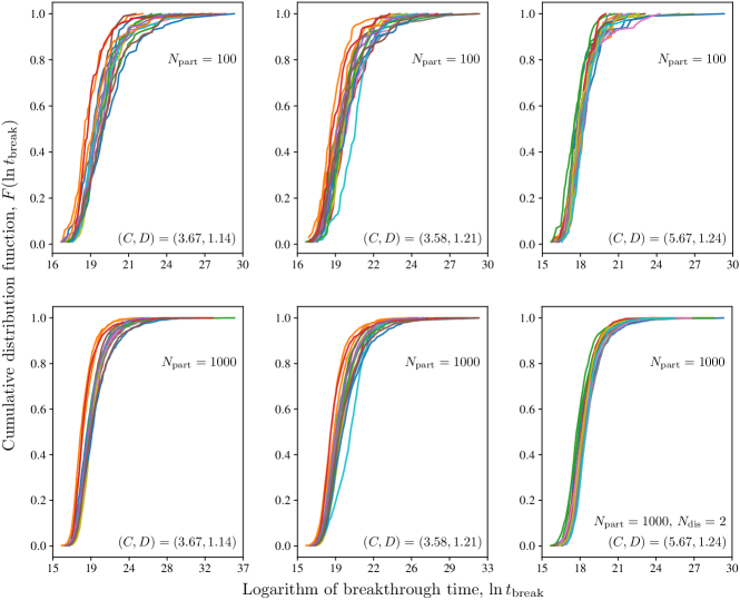
Figure 1: Representative CDFs of the logarithm of breakthrough times (in seconds) of $N_{\text{part}}$ particles, $F(\ln t_{\text{break}})$, for 20 realizations of the DFN characterized by a given combination of the DFN parameters $(C,D)$. Each colored curve corresponds to a different random realization; in all simulations, we set $p_{\text{lim}}=0.5$.

In addition to $N_{\text{part}}$, the simulation time and accuracy of each forward model run are largely controlled by the number of elements used to discretize a fracture, which is defined by the parameter $p_{\text{lim}}$ introduced in section 2.3. The simulation time $t_{\text{sim}}$ refers to the time (in seconds) it takes to estimate the CDF of breakthrough times for one random DFN realization and one of the $N_{\text{sim}}=10^{4}$ pairs of the parameters $(C,D)$. We found the average $t_{\text{sim}}$ not to exceed 1 s if either $N_{\text{part}}=100$ or the fracture is not discretized (Table 1 of the Supplemental Material); the average is over 20 random realizations of the DFN obtained with different random seeds for each parameter pair $(C,D)$.

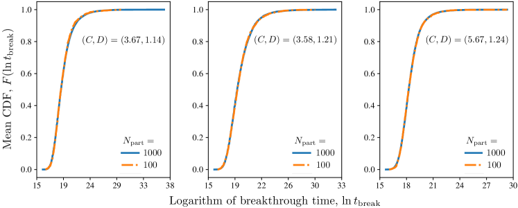
Figure 2: Mean CDFs of the logarithm of breakthrough times (in seconds) of $N_{\text{part}}$ particles, $F(\ln t_{\text{break}})$, averaged over the corresponding DFN realizations in Figure 1.

Representative CDFs of breakthrough times of $N_{\text{part}}$ particles, in each of these 20 DFN realizations, are displayed in Figure 1 for three pairs of the DFN parameters $(C,D)$. The across-realization variability of the CDFs is more pronounced for $N_{\text{part}}=10^{2}$ then $10^{3}$ particles, and visually indistinguishable when going from $N_{\text{part}}=10^{3}$ to $10^{4}$ particles (not shown here). Likewise, no appreciable differences between the CDFs computed with $p_{\text{lim}}=0.5$ and $0.2$ were observed. Finally, when the random-seed effects are averaged out, the resulting breakthrough-time CDFs for $N_{\text{part}}=10^{2}$ and $10^{3}$ are practically identical (Figure 2). Based on these findings, in the subsequent simulations, we set $N_{\text{part}}=100$ and $p_{\text{lim}}=0.5$ in order to obtain an optimal balance between the computational time and accuracy.

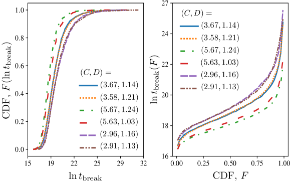
Figure 3: CDFs (left) and corresponding iCDFs (right) of the thermal breakthrough times for a single realization of the six DFNs characterized by six pairs of the parameters $(C,D)$.

For some parameter pairs $(C,D)$, not every DFN realization (defined by the random seed) hydraulically connects the injection and observation boundaries. Such hydraulically disconnected networks are not suitable for our flow model (see section 2.2). However, in our numerical experiments, there were at least 10—and, in the majority of cases, 19—connected fracture networks for each $(C,D)$ pair (Figure 2 of the Supplemental Material).

The final step in our data generation procedure consists of converting the estimated CDFs $F$ into corresponding iCDFs $F^{-1}$ (Figure 3). The latter form the data set $\mathbf{d}$, different parts of which are used to train a CNN and to verify its performance.

5.3 CNN training and testing

The data generated above are arranged in a set $\{\mathbf{m}_{\text{NN}_{i}},\mathbf{d}_{i}\}_{i=1}^{N_{\text{sim}}}$ with $N_{\text{sim}}=10^{4}$ and $\mathbf{m}_{\text{NN}}$ defined in (9). We randomly select $8\cdot 10^{3}$ of these pairs to train the FCNN $\mathbf{NN}$ in (5), leaving the remaining $2\cdot 10^{3}$ for testing. The output data $\mathbf{d}$ come in the form of iCDFs, i.e., non-decreasing series of numbers. Since a NN model is not guaranteed to reproduce this trend, we use the hyper-parameter tuning method [Liaw . (2018)] to perform the search in the hyper-parameter space specified in Table 1.

Table 1: Hyper-parameter search space defined by the number of layers, the number of neurons in each layer, the optimizer names, and (logarithm of) the learning rate. These parameters are uniformly sampled from either a discrete set of values, $\mathcal{U}\{\cdot,\cdot,\dots,\cdot\}$, or an interval, $\mathcal{U}[\cdot,\cdot]$. The RMSprop optimizer [Graves (2013), Hinton . (2012)], rms; the stochastic gradient descent optimizer [Sutskever . (2013)], sgd; the Adagrad optimizer [Duchi . (2011)] ada; and the Adam optimizer [Kingma  Ba (2014)], adam, slightly differ from each other when performing the parameter gradient descent during the NN training.

Parameter name	Search region
Number of layers	$\mathcal{U}\{3,4,5,6\}$
Number of neurons	$\mathcal{U}\{2^{2},2^{3},...,2^{9}\}$
Optimizer name	$\mathcal{U}\{\texttt{rms},\texttt{sgd},\texttt{ada},\texttt{adam}\}$
Learning rate, $l_{r}$	$\log_{10}(l_{r})\sim\mathcal{U}[-4,-2]$

The hyper-parameter search involved 2500 trials; in each trial, the subset of data $\{\mathbf{m}_{\text{NN}_{i}},$ $\mathbf{d}_{i}\}_{i=1}^{8000}$ were randomly split into a training set consisting of 6400 pairs $\{\mathbf{m}_{\text{NN}_{i}},\mathbf{d}_{i}\}$ and a validation set comprising the remaining 1600 pairs $\{\mathbf{m}_{\text{NN}_{i}},\mathbf{d}_{i}\}$. For each epoch, the 6400 training pairs were used to optimize the NN parameters, and the NN accuracy is evaluated on the validation set. Each trial used one of the optimizers in Table 1 for at most $10^{3}$ epochs; the trial was stopped if the validation loss did not decrease for $10^{2}$ epochs. After completion of all the trials with these rules, the trial with the smallest validation loss was saved. The optimal FCNN, described in Table 2, has 6 layers between the input and output layers and is obtained using the Adam optimizer with the Adam optimizer coefficients $\beta=(0.9,0.999)$ to perform gradient descent. This trial is associated with a learning rate $l_{r}=0.00403$ and the averaged Hellinger loss of $0.0827$ on the validation set. This FCNN was further trained with a learning rate that reduces on plateau of the validation performance to further fine-tune the model parameters for another $10^{3}$ epochs; the ending testing Hellinger loss is $0.0652$ and the total training time is $37340$ seconds. Figure 4 depicts the FCNN predictions of the iCDFs of the particle breakthrough times in DFNs characterized by different parameter-pairs $(C,D)$ not used for training. These predictions are visually indistinguishable from those obtained with the physics-based model $\mathbf{g}(\mathbf{m})$ described in section 2.1.

Table 2: The best-trial NN architecture consists of six hidden layers, $FC_{i}$ ($i=1,\dots,6$), with the corresponding weight matrix $\mathbf{W}_{i}$ and layer output $\mathbf{s}_{i}$ ($i=1,\dots,6$) in (6). Bias parameters are added to each layer, but not shown in this table.

Layer	Weights	Layer output
Input	-	6
$FC_{1}$	$\mathbf{W}_{1}:256\times 6$	$\mathbf{s}_{1}:256$
$FC_{2}$	$\mathbf{W}_{2}:64\times 256$	$\mathbf{s}_{2}:64$
$FC_{3}$	$\mathbf{W}_{3}:512\times 64$	$\mathbf{s}_{3}:512$
$FC_{4}$	$\mathbf{W}_{4}:256\times 512$	$\mathbf{s}_{4}:256$
$FC_{5}$	$\mathbf{W}_{5}:32\times 256$	$\mathbf{s}_{5}:32$
$FC_{6}$	$\mathbf{W}_{6}:128\times 32$	$\mathbf{s}_{6}:128$
Output	$\mathbf{W}_{7}:50\times 128$	$50$

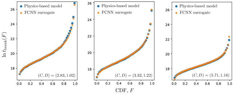
Figure 4: Physics-based and FCNN predictions of the iCDFs of the particle breakthrough times in DFNs characterized by different parameter-pairs $(C,D)$ not used for training.

5.4 Bayesian inversion without prior information

We start with the Bayesian data assimilation and parameter estimation from section 4. Taking the uniform prior, $\gamma=0$ in (13), and assimilating the $N_{\text{sim}}=10^{4}$ candidates provided by the physics-based model $\mathbf{g}$, this procedure yields the posterior PDFs of $C$ and $D$ shown in Figure 5. While this non-informative prior indicates that all values of the parameters $(C,D)$ are equally likely, the sharpened posterior correctly assigns higher probability to the region containing the reference $(C,D)$ values. The relatively small number ($N_{\text{sim}}=10^{4}$) of the forward solves of the physics-based model $\mathbf{g}$ manifests itself in granularity of the posterior PDF maps.

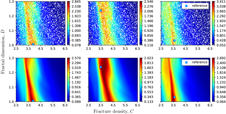
Figure 5: Examples of posterior PDFs of the DFN parameters $C$ and $D$, for three experiments defined by the reference parameter values (blue circles). These PDFs are computed via Bayesian assimilation of either $10^{4}$ runs of the physics-based model (top row) or additional $10^{7}$ runs of the FCNN surrogate (bottom row).

Significantly more forward model runs are needed to further sharpen these posterior PDFs around the true values of $(C,D)$ and to reduce the image pixelation. Generating the significant amounts of such data with the physics-based model is computationally prohibitive. Instead, we use $10^{7}$ additional candidates, corresponding to a $10^{4}\times 10^{3}$ mesh of the parameter space, provided by the FCNN surrogate. Figure 5 demonstrates that assimilation of these data (forward runs of the cheap FCNN surrogate) further reduces the band containing the unknown model parameters $(C,D)$ with high probability. Generation of such large data sets with the physics-based model is four orders of magnitude more expensive than that with the FCNN.

Table 3: Computational cost of the Bayesian inversion using the physics-based model $\mathbf{g}(\mathbf{m})$ or the FCNN surrogate $\mathbf{NN(\mathbf{m})}$. Each inversion requires $N_{\text{sim}}$ forward runs and takes time $T_{\text{tot}}$. The latter comprises time to train the model ($T_{\text{train}}$), time to execute the forward runs ($T_{\text{run}}$) and time to define the posterior PDF on the discretized parameter grid ($T_{\text{grid}}$). The running time for $\mathbf{g}(\mathbf{m})$ is a projection based on the simulation time of $6560$ seconds that was necessary to run $10^{4}$ simulations. The FCNN was trained and executed on GPUs provided by GoogleColab. All times are in seconds.

	$N_{\text{sim}}$	$T_{\text{train}}$	$T_{\text{run}}$	$T_{\text{grid}}$	$T_{\text{tot}}$
$\mathbf{g}(\mathbf{m})$	$2\times 10^{8}$	$0$	$1.312\cdot 10^{8}$	$5.47$	$1.312\cdot 10^{8}$
$\mathbf{NN}(\mathbf{m})$	$10^{7}$	$37340$	$1.26$	$5.47$	$3.735\cdot 10^{4}$

The posterior PDFs displayed in Figure 5 show that the fracture density $C$ is well constrained and amenable to our Bayesian inversion, whereas the inference of the fractal dimension $D$ is more elusive. Examples of the DFNs in this study are provided in Figure 2 of [Gisladottir . (2016)]. They suggest that, for the parameter ranges considered, $C$ impacts the spatial extent of a fracture network, while $D$ affects the fracture-length distribution. Consequently, $C$ has a more significant impact on the overall structures.

5.5 Bayesian inversion with data-informed priors

To refine the inference of parameters $C$ and $D$ from the breakthrough-time CDFs, we add some prior information. First, we observe that the field data reported in A suggest that $C$ and $D$ are correlated. These data are fitted with a shallow feed-forward NN resulting in the prior PDF of $C$ and $D$ shown in Figure 6. These data vary over larger ranges than those used for $C$ and $D$ in the previous section; at the same time, most values correspond to $C<2$. That is because the field data come from a large number of different sites and from direct outcrop observations. Figure 9 in [Watanabe  Takahashi (1995)] shows that a network with $C<2$ would have low connectivity. On the other hand, a DFN with a large $D$ is very dense, requiring large computational times to simulate and, possibly, being amenable to a (stochastic) continuum representation. Driven by these practical considerations, and to ascertain the value of this additional information, we restrict the prior PDF from Figure 6 to the same range of parameters as that used in the previous section.

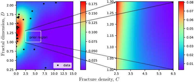
Figure 6: Prior joint PDF of $C$ and $D$ inferred from the field-scale data in A (left) and its rescaled counterpart over the parameter range used in our study (right).

The relative importance given to the prior information about the DFN properties $C$ and $D$ (Figure 6) is controlled by the parameter $\gamma$ in (12). Large values of $\gamma$ correspond to higher confidence in the quality and relevance of the data reported in A. Figure 7 exhibits posterior PDFs of $C$ and $D$ computed via our Bayesian assimilation procedure with $\gamma=0.5$ and 1. Visual comparison of Figures 5 and 7 reveals that the incorporation of the prior information about generic (not site-specific) correlations between $C$ and $D$ sharpens our estimation of these parameters, i.e., decreases the area in the parameter space where they are predicted to lie with high probability. Putting more trust in the prior, i.e., using a higher value of $\gamma$, amplifies this trend. However, the increase in certainty might be misplaced, as witnessed by several examples the reference parameter values fall outside the high probability regions.

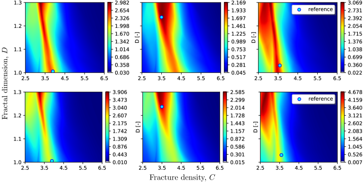
Figure 7: Examples of posterior PDFs of the DFN parameters $C$ and $D$ in the presence of prior information, for three experiments defined by the reference parameter values (blue circles). These PDFs are computed via Bayesian assimilation with the informative prior (Figure 6), whose relative importance increases from $\gamma=0.5$ (top) to $\gamma=1.0$ (bottom).

Fracture network’s connectivity is another potential source of information that can boost one’s ability to infer the parameters $C$ and $D$ from CBTEs. Let $N_{\text{con}_{i}}$ denote the number of connected fracture networks among 20 random realizations of a DFN characterized by $(C,D)_{i}$. Figure 8 exhibits $N_{\text{con}_{i}}$ for $N_{\text{sim}}=10^{4}$ DFNs characterized by $(C,D)_{i}$ ($i=1,\dots,N_{\text{sim}}$), with the results interpolated to $10^{4}\times 10^{3}$ mesh of the $(C,D)$ space by means of a shallow NN. We define a prior PDF for $C$ and $D$ as

$$f_{\textbf{m}}(\tilde{\mathbf{m}})\propto N^{2}_{\text{con}}(\tilde{\mathbf{m}}),\quad N_{\text{con}}\in[0,1,\dots,20],$$ (14)

which is properly normalized to ensure it integrates to one. This prior PDF, shown in Figure 8, assigns larger probability to those $(C,D)$ pairs that show higher connectivity in our data set.

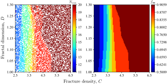
Figure 8: Number of connected networks, $N_{\text{con}}$, averaged over 20 random realizations of the DFN model with a given parameter pair $\mathbf{m}=(C,D)^{\top}$ (left); and corresponding prior PDF $f_{\mathbf{m}}$ in (14) (right).

The Bayesian inference procedure with this prior yields the posterior joint PDFs of $C$ and $D$ in Figure 9. These distributions are sharper than those computed with either uninformative (Figure 5) or correlation-based (Figure 7) priors, indicating the further increased confidence in the method’s predictions of $C$ and $D$. As before, assigning more weight to the prior, i.e., increasing $\gamma$, reduces the area of the high-probability regions in the $(C,D)$ space. This increased confidence in predictions of $C$ and $D$ is more pronounced when the connectivity-based prior, rather than the correlation-based prior, is used. The connectivity information also ensures that this confidence is not misplaced, i.e., the reference parameter values lie within the high-probability regions.

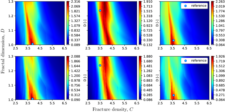
Figure 9: Examples of posterior PDFs of the DFN parameters $C$ and $D$ in the presence of prior information, for three experiments defined by the reference parameter values (blue circles). These PDFs are computed via Bayesian assimilation with the informative prior (14), whose relative importance increases from $\gamma=0.5$ (top) to $\gamma=1.0$ (bottom).

6 Conclusions

We developed and applied a computationally efficient parameter-estimation method, which makes it possible to infer the statistical properties of a fracture network from cross-borehole thermal experiments (CBTEs). A key component of our method is the construction of a neural network surrogate of the physics-based model of fluid flow and heat transfer in fractured rocks. The negligible computational cost of this surrogate allows for the deployment of a straightforward grid search in the parameter space spanned by fracture density $C$ and fractal dimension $D$. Our numerical experiments lead to the following major conclusions.

1. The neural network surrogate provides accurate estimates of an average inverse cumulative distribution function (iCDF) of breakthrough times, for the fracture network characterized by given parameters $(C,D)$.

2. In the absence of any expert knowledge about $C$ and $D$, i.e., when an uninformative prior is used, our method—with the likelihood function defined in terms of the Hellinger distance between the predicted and observed iCDFs—significantly sharpens this prior, correctly identifying parameter regions wherein the true values of $(C,D)$ lie.

3. Incorporation of the prior information about generic (not site-specific) correlations between $C$ and $D$ sharpens our estimation of these parameters, i.e., decreases the area in the parameter space where they are predicted to lie with high probability. Putting more trust in the prior, i.e., using a higher value of $\gamma$, amplifies this trend. However, the increase in certainty might be misplaced, as witnessed by several examples the reference parameter values fall outside the high probability regions.

4. Incorporation of the prior information about a fracture network’s connectivity yields the posterior joint PDFs of $C$ and $D$ that are sharper than those computed with either uninformative or correlation-based priors, indicating the further increased confidence in the method’s predictions of $C$ and $D$.

5. The increased confidence in predictions of $C$ and $D$ is more pronounced when the connectivity-based prior, rather than the correlation-based prior, is used. The connectivity information also ensures that this confidence is not misplaced, i.e., the reference parameter values lie within the high-probability regions.

Appendix A Field-scale characterization of fracture networks

For the sake of completeness, we report in Table LABEL:tab:appA1 the field-scale observations of fracture networks from [Bonnet . (2001)]. These are accompanied by our calculation of the corresponding values of parameters $C$ and $D$ in the WT model of fracture networks.

Table A.1: Fracture number ($N_{\text{f}}$), power-law exponent ($a$), surface area ($S$), minimum fracture length ($l_{\text{min}}$), and density parameter $\alpha$ for various fracture networks reported in Table 2 in [Bonnet . (2001)]. The corresponding values of fracture density ($C$) and fractal dimension ($D$) in the WT network model (1) are determined from the parameter relationships in Section 2.1.

$N_{\text{f}}$ [-]	$a$ [-]	$S$ [m2]	$l_{\text{min}}$ [m]	$\alpha$ [-]	$D$ [-]	$C$ [-]
107	1.74	24	0.1	0.60035	0.74	86.80731
121	2.11	25	0.1	0.41703	1.11	45.46014
3499	1.88	2.70$\cdot 10^{11}$	$10^{3}$	4.97809$\cdot 10^{-6}$	0.88	0.01979
120	0.9	8.25$\cdot 10^{7}$	40	-1.00582$\cdot 10^{-7}$	-0.1	0.00012
101	1	2.62$\cdot 10^{7}$	57	0	0	NaN
300	1.76	NP	7.00$\cdot 10^{3}$	NaN	0.76	NaN
380	1.9	3.43$\cdot 10^{3}$	3	0.26777	0.9	113.05832
350	2.1	1.26$\cdot 10^{8}$	220	0.00115	1.1	0.36680
1000	3.2	1.60$\cdot 10^{9}$	380	0.65137	2.2	296.07649
1000	2.1	1.65$\cdot 10^{10}$	2.00$\cdot 10^{3}$	0.00028	1.1	0.25921
800	2.2	2.50$\cdot 10^{1}$	6.00$\cdot 10^{-2}$	1.31254	1.2	875.02702
380	2.1	NP	2.50$\cdot 10^{3}$	NaN	1.1	NaN
1700	2.02	1.00$\cdot 10^{10}$	1.00$\cdot 10^{3}$	0.0002	1.02	0.33182
260	1.3	8.75$\cdot 10^{3}$	1.00	0.00891	0.3	7.72571
100	1.8	2.10$\cdot 10^{3}$	1.00	0.03809	0.8	4.76190
873	2.64	3.40$\cdot 10^{1}$	5.00$\cdot 10^{-3}$	0.00709	1.64	3.7745
320	2.61	2.07$\cdot 10^{7}$	4.00$\cdot 10$	0.00945	1.61	1.87779
50	1.67	2.90$\cdot 10^{7}$	7.00$\cdot 10$	1.99004$\cdot 10^{-5}$	0.67	0.00148
180	1.97	2.80$\cdot 10^{8}$	3.00$\cdot 10^{2}$	0.00016	0.97	0.02925
400	2.21	1.20$\cdot 10^{8}$	4.00$\cdot 10$	0.00035	1.21	0.11573
250	2.11	2.50$\cdot 10^{11}$	4.50$\cdot 10^{3}$	1.26005$\cdot 10^{-5}$	1.11	0.00284
400	2.84	2.90$\cdot 10^{11}$	5.50$\cdot 10^{3}$	0.01935	1.84	4.20716
70	2.67	3.60$\cdot 10^{9}$	1.60$\cdot 10^{3}$	0.00728	1.67	0.30533
150	2.66	5.10$\cdot 10^{9}$	1.25$\cdot 10^{3}$	0.00675	1.66	0.61021
200	3.07	6.20$\cdot 10^{9}$	1.00$\cdot 10^{3}$	0.10829	2.07	10.46329
1034	2.51	8.70$\cdot 10^{7}$	1.00$\cdot 10$	0.00058	1.51	0.39767
40	1.6	2.00$\cdot 10^{4}$	6.00$\cdot 10^{-2}$	0.00022	0.6	0.01479
318	2.42	1.69$\cdot 10^{8}$	7.00$\cdot 10$	0.00111	1.42	0.24946
291	2.69	1.69$\cdot 10^{8}$	7.00$\cdot 10$	0.00382	1.69	0.65783
78	2.1	1.69$\cdot 10^{8}$	1.00$\cdot 10^{2}$	8.04638$\cdot 10^{-5}$	1.1	0.00570
218	2.02	1.00	2.00$\cdot 10^{-2}$	4.11251	1.02	878.94881
111	3.04	8.40$\cdot 10^{7}$	2.00$\cdot 10^{2}$	0.13328	2.04	7.25217
470	1.8	1.17$\cdot 10^{4}$	6.00$\cdot 10^{-2}$	0.00338	0.8	1.98852
417	2.18	6.00$\cdot 10^{7}$	4.00$\cdot 10$	0.00064	1.18	0.22519
201	2.4	3.00E-01	1.50E-04	0.00416	1.4	0.59676
100	2.4	6.00$\cdot 10^{8}$	7.00$\cdot 10^{2}$	0.00224	1.4	0.16032
1034	2.36	8.70$\cdot 10^{7}$	1.00$\cdot 10$	0.00037	1.36	0.28153
450	2.18	2.20$\cdot 10^{8}$	7.00$\cdot 10$	0.00036	1.18	0.13843
350	2.75	1.50$\cdot 10^{9}$	1.80$\cdot 10^{2}$	0.00361	1.75	0.72239
300	2.37	NP	1.00$\cdot 10^{2}$	NaN	1.37	NaN

References

- Agarap (\APACyear2018) \APACinsertmetastaragarap2018deep{APACrefauthors}Agarap, A\BPBIF. \APACrefYearMonthDay2018. \BBOQ\APACrefatitleDeep learning using rectified linear units (relu) Deep learning using rectified linear units (relu).\BBCQ \APACjournalVolNumPagesarXiv preprint arXiv:1803.08375. \PrintBackRefs\CurrentBib
- Akoachere \BBA Van Tonder (\APACyear2011) \APACinsertmetastarAkoachere2011{APACrefauthors}Akoachere, R\BPBIA., II\BCBT \BBA Van Tonder, G. \APACrefYearMonthDay2011APR. \BBOQ\APACrefatitleThe trigger-tube: A new apparatus and method for mixing solutes for injection tests in boreholes The trigger-tube: A new apparatus and method for mixing solutes for injection tests in boreholes.\BBCQ \APACjournalVolNumPagesWater SA372139-146. \PrintBackRefs\CurrentBib
- Barajas-Solano \BOthers. (\APACyear2019) \APACinsertmetastarbarajas2019efficient{APACrefauthors}Barajas-Solano, D\BPBIA., Alexander, F\BPBIJ., Anghel, M.\BCBL \BBA Tartakovsky, D\BPBIM. \APACrefYearMonthDay2019. \BBOQ\APACrefatitleEfficient gHMC reconstruction of contaminant release history Efficient ghmc reconstruction of contaminant release history.\BBCQ \APACjournalVolNumPagesFrontiers in Environmental Science7149. \PrintBackRefs\CurrentBib
- Bonnet \BOthers. (\APACyear2001) \APACinsertmetastarBonnet2001{APACrefauthors}Bonnet, E., Bour, O., Odling, N\BPBIE., Davy, P., Main, I., Cowie, P.\BCBL \BBA Berkowitz, B. \APACrefYearMonthDay2001. \BBOQ\APACrefatitleScaling of fracture systems in geological media Scaling of fracture systems in geological media.\BBCQ \APACjournalVolNumPagesReviews of Geophysics393347-383. {APACrefURL} http://dx.doi.org/10.1029/1999RG000074 {APACrefDOI} 10.1029/1999RG000074 \PrintBackRefs\CurrentBib
- Boso \BBA Tartakovsky (\APACyear2020\APACexlab\BCnt1) \APACinsertmetastarboso-2020-data{APACrefauthors}Boso, F.\BCBT \BBA Tartakovsky, D\BPBIM. \APACrefYearMonthDay2020\BCnt1. \BBOQ\APACrefatitleData-informed method of distributions for hyperbolic conservation laws Data-informed method of distributions for hyperbolic conservation laws.\BBCQ \APACjournalVolNumPagesSIAM J. Sci. Comput.421A559-A583. {APACrefDOI} 10.1137/19M1260773 \PrintBackRefs\CurrentBib
- Boso \BBA Tartakovsky (\APACyear2020\APACexlab\BCnt2) \APACinsertmetastarboso-2020-learning{APACrefauthors}Boso, F.\BCBT \BBA Tartakovsky, D\BPBIM. \APACrefYearMonthDay2020\BCnt2. \BBOQ\APACrefatitleLearning on dynamic statistical manifolds Learning on dynamic statistical manifolds.\BBCQ \APACjournalVolNumPagesProc. Roy. Soc. A476223920200213. {APACrefDOI} 10.1098/rspa.2020.0213 \PrintBackRefs\CurrentBib
- Ciriello \BOthers. (\APACyear2019) \APACinsertmetastarciriello-2019-distribution{APACrefauthors}Ciriello, V., Lauriola, I.\BCBL \BBA Tartakovsky, D\BPBIM. \APACrefYearMonthDay2019. \BBOQ\APACrefatitleDistribution-based global sensitivity analysis in hydrology Distribution-based global sensitivity analysis in hydrology.\BBCQ \APACjournalVolNumPagesWater Resour. Res.55118708-8720. {APACrefDOI} 10.1029/2019WR025844 \PrintBackRefs\CurrentBib
- Davy \BOthers. (\APACyear1990) \APACinsertmetastardavy1990some{APACrefauthors}Davy, P., Sornette, A.\BCBL \BBA Sornette, D. \APACrefYearMonthDay1990. \BBOQ\APACrefatitleSome consequences of a proposed fractal nature of continental faulting Some consequences of a proposed fractal nature of continental faulting.\BBCQ \APACjournalVolNumPagesNature348629656–58. \PrintBackRefs\CurrentBib
- de La Bernardie \BOthers. (\APACyear2018) \APACinsertmetastarde2018thermal{APACrefauthors}de La Bernardie, J., Bour, O., Le Borgne, T., Guihéneuf, N., Chatton, E., Labasque, T.\BDBLGerard, M\BHBIF. \APACrefYearMonthDay2018. \BBOQ\APACrefatitleThermal attenuation and lag time in fractured rock: Theory and field measurements from joint heat and solute tracer tests Thermal attenuation and lag time in fractured rock: Theory and field measurements from joint heat and solute tracer tests.\BBCQ \APACjournalVolNumPagesWater Resources Research541210–053. \PrintBackRefs\CurrentBib
- Demirel \BOthers. (\APACyear2018) \APACinsertmetastardemirel2018characterizing{APACrefauthors}Demirel, S., Roubinet, D., Irving, J.\BCBL \BBA Voytek, E. \APACrefYearMonthDay2018. \BBOQ\APACrefatitleCharacterizing near-surface fractured-rock aquifers: Insights provided by the numerical analysis of electrical resistivity experiments Characterizing near-surface fractured-rock aquifers: Insights provided by the numerical analysis of electrical resistivity experiments.\BBCQ \APACjournalVolNumPagesWater1091117. \PrintBackRefs\CurrentBib
- Dorn \BOthers. (\APACyear2013) \APACinsertmetastarDorn2013{APACrefauthors}Dorn, C., Linde, N., Le Borgne, T., Bour, O.\BCBL \BBA de Dreuzy, J\BHBIR. \APACrefYearMonthDay2013. \BBOQ\APACrefatitleConditioning of stochastic 3-D fracture networks to hydrological and geophysical data Conditioning of stochastic 3-d fracture networks to hydrological and geophysical data.\BBCQ \APACjournalVolNumPagesAdvances in Water Resources62, Part A079-89. {APACrefURL} http://www.sciencedirect.com/science/article/pii/S0309170813001863 {APACrefDOI} 10.1016/j.advwatres.2013.10.005 \PrintBackRefs\CurrentBib
- Dorn \BOthers. (\APACyear2012) \APACinsertmetastardorn2012inferring{APACrefauthors}Dorn, C., Linde, N., Le Borgne, T., Bour, O.\BCBL \BBA Klepikova, M. \APACrefYearMonthDay2012. \BBOQ\APACrefatitleInferring transport characteristics in a fractured rock aquifer by combining single-hole ground-penetrating radar reflection monitoring and tracer test data Inferring transport characteristics in a fractured rock aquifer by combining single-hole ground-penetrating radar reflection monitoring and tracer test data.\BBCQ \APACjournalVolNumPagesWater Resources Research4811. \PrintBackRefs\CurrentBib
- Duchi \BOthers. (\APACyear2011) \APACinsertmetastarduchi2011adaptive{APACrefauthors}Duchi, J., Hazan, E.\BCBL \BBA Singer, Y. \APACrefYearMonthDay2011. \BBOQ\APACrefatitleAdaptive subgradient methods for online learning and stochastic optimization. Adaptive subgradient methods for online learning and stochastic optimization.\BBCQ \APACjournalVolNumPagesJournal of machine learning research127. \PrintBackRefs\CurrentBib
- Fischer \BOthers. (\APACyear2018) \APACinsertmetastarfischer2018hydraulic{APACrefauthors}Fischer, P., Jardani, A.\BCBL \BBA Lecoq, N. \APACrefYearMonthDay2018. \BBOQ\APACrefatitleHydraulic tomography of discrete networks of conduits and fractures in a karstic aquifer by using a deterministic inversion algorithm Hydraulic tomography of discrete networks of conduits and fractures in a karstic aquifer by using a deterministic inversion algorithm.\BBCQ \APACjournalVolNumPagesAdvances in water resources11283–94. \PrintBackRefs\CurrentBib
- Gisladottir \BOthers. (\APACyear2016) \APACinsertmetastargisladottir2016particle{APACrefauthors}Gisladottir, V\BPBIR., Roubinet, D.\BCBL \BBA Tartakovsky, D\BPBIM. \APACrefYearMonthDay2016. \BBOQ\APACrefatitleParticle methods for heat transfer in fractured media Particle methods for heat transfer in fractured media.\BBCQ \APACjournalVolNumPagesTransport in Porous Media1152311–326. \PrintBackRefs\CurrentBib
- Goodfellow \BOthers. (\APACyear2014) \APACinsertmetastargoodfellow2014generative{APACrefauthors}Goodfellow, I\BPBIJ., Pouget-Abadie, J., Mirza, M., Xu, B., Warde-Farley, D., Ozair, S.\BDBLBengio, Y. \APACrefYearMonthDay2014. \BBOQ\APACrefatitleGenerative adversarial networks Generative adversarial networks.\BBCQ \APACjournalVolNumPagesarXiv preprint arXiv:1406.2661. \PrintBackRefs\CurrentBib
- Graves (\APACyear2013) \APACinsertmetastargraves2013generating{APACrefauthors}Graves, A. \APACrefYearMonthDay2013. \BBOQ\APACrefatitleGenerating sequences with recurrent neural networks Generating sequences with recurrent neural networks.\BBCQ \APACjournalVolNumPagesarXiv preprint arXiv:1308.0850. \PrintBackRefs\CurrentBib
- Haddad \BOthers. (\APACyear2014) \APACinsertmetastarhaddad2014application{APACrefauthors}Haddad, A\BPBIS., Hassanzadeh, H., Abedi, J.\BCBL \BBA Chen, Z. \APACrefYearMonthDay2014. \BBOQ\APACrefatitleApplication of tracer injection tests to characterize rock matrix block size distribution and dispersivity in fractured aquifers Application of tracer injection tests to characterize rock matrix block size distribution and dispersivity in fractured aquifers.\BBCQ \APACjournalVolNumPagesJournal of Hydrology510504–512. \PrintBackRefs\CurrentBib
- Hinton \BOthers. (\APACyear2012) \APACinsertmetastarhinton2012neural{APACrefauthors}Hinton, G., Srivastava, N.\BCBL \BBA Swersky, K. \APACrefYearMonthDay2012. \BBOQ\APACrefatitleNeural networks for machine learning lecture 6a overview of mini-batch gradient descent Neural networks for machine learning lecture 6a overview of mini-batch gradient descent.\BBCQ \APACjournalVolNumPagesCited on148. \PrintBackRefs\CurrentBib
- I. Jang \BOthers. (\APACyear2008) \APACinsertmetastarjang2008inverse{APACrefauthors}Jang, I., Kang, J.\BCBL \BBA Park, C. \APACrefYearMonthDay2008. \BBOQ\APACrefatitleInverse fracture model integrating fracture statistics and well-testing data Inverse fracture model integrating fracture statistics and well-testing data.\BBCQ \APACjournalVolNumPagesEnergy Sources, Part A30181677–1688. \PrintBackRefs\CurrentBib
- Y\BPBIH. Jang \BOthers. (\APACyear2013) \APACinsertmetastarjang2013oil{APACrefauthors}Jang, Y\BPBIH., Lee, T\BPBIH., Jung, J\BPBIH., Kwon, S\BPBII.\BCBL \BBA Sung, W\BPBIM. \APACrefYearMonthDay2013. \BBOQ\APACrefatitleThe oil production performance analysis using discrete fracture network model with simulated annealing inverse method The oil production performance analysis using discrete fracture network model with simulated annealing inverse method.\BBCQ \APACjournalVolNumPagesGeosciences Journal174489–496. \PrintBackRefs\CurrentBib
- Kang \BOthers. (\APACyear2021) \APACinsertmetastarkang2021hydrogeophysical{APACrefauthors}Kang, X., Kokkinaki, A., Kitanidis, P\BPBIK., Shi, X., Lee, J., Mo, S.\BCBL \BBA Wu, J. \APACrefYearMonthDay2021. \BBOQ\APACrefatitleHydrogeophysical Characterization of Nonstationary DNAPL Source Zones by Integrating a Convolutional Variational Autoencoder and Ensemble Smoother Hydrogeophysical characterization of nonstationary DNAPL source zones by integrating a convolutional variational autoencoder and ensemble smoother.\BBCQ \APACjournalVolNumPagesWater Resources Research572e2020WR028538. \PrintBackRefs\CurrentBib
- Kingma \BBA Ba (\APACyear2014) \APACinsertmetastarkingma2014adam{APACrefauthors}Kingma, D\BPBIP.\BCBT \BBA Ba, J. \APACrefYearMonthDay2014. \BBOQ\APACrefatitleAdam: A method for stochastic optimization Adam: A method for stochastic optimization.\BBCQ \APACjournalVolNumPagesarXiv preprint arXiv:1412.6980. \PrintBackRefs\CurrentBib
- Kingma \BBA Welling (\APACyear2013) \APACinsertmetastarkingma2013auto{APACrefauthors}Kingma, D\BPBIP.\BCBT \BBA Welling, M. \APACrefYearMonthDay2013. \BBOQ\APACrefatitleAuto-encoding variational bayes Auto-encoding variational bayes.\BBCQ \APACjournalVolNumPagesarXiv preprint arXiv:1312.6114. \PrintBackRefs\CurrentBib
- Klepikova \BOthers. (\APACyear2013) \APACinsertmetastarKlepikova2013{APACrefauthors}Klepikova, M\BPBIV., Le Borgne, T., Bour, O.\BCBL \BBA de Dreuzy, J\BHBIR. \APACrefYearMonthDay2013NOV. \BBOQ\APACrefatitleInverse modeling of flow tomography experiments in fractured media Inverse modeling of flow tomography experiments in fractured media.\BBCQ \APACjournalVolNumPagesWater Resources Research49117255-7265. {APACrefDOI} 10.1002/2013WR013722 \PrintBackRefs\CurrentBib
- Klepikova \BOthers. (\APACyear2016) \APACinsertmetastarklepikova2016heat{APACrefauthors}Klepikova, M\BPBIV., Le Borgne, T., Bour, O., Dentz, M., Hochreutener, R.\BCBL \BBA Lavenant, N. \APACrefYearMonthDay2016. \BBOQ\APACrefatitleHeat as a tracer for understanding transport processes in fractured media: Theory and field assessment from multiscale thermal push-pull tracer tests Heat as a tracer for understanding transport processes in fractured media: Theory and field assessment from multiscale thermal push-pull tracer tests.\BBCQ \APACjournalVolNumPagesWater Resources Research5275442–5457. \PrintBackRefs\CurrentBib
- Klepikova \BOthers. (\APACyear2014) \APACinsertmetastarklepikova2014passive{APACrefauthors}Klepikova, M\BPBIV., Le Borgne, T., Bour, O., Gallagher, K., Hochreutener, R.\BCBL \BBA Lavenant, N. \APACrefYearMonthDay2014. \BBOQ\APACrefatitlePassive temperature tomography experiments to characterize transmissivity and connectivity of preferential flow paths in fractured media Passive temperature tomography experiments to characterize transmissivity and connectivity of preferential flow paths in fractured media.\BBCQ \APACjournalVolNumPagesJournal of Hydrology512549–562. \PrintBackRefs\CurrentBib
- Kullback (\APACyear1997) \APACinsertmetastarkullback1997information{APACrefauthors}Kullback, S. \APACrefYear1997. \APACrefbtitleInformation theory and statistics Information theory and statistics. \APACaddressPublisherCourier Corporation. \PrintBackRefs\CurrentBib
- Le Cam (\APACyear2012) \APACinsertmetastarle2012asymptotic{APACrefauthors}Le Cam, L. \APACrefYear2012. \APACrefbtitleAsymptotic methods in statistical decision theory Asymptotic methods in statistical decision theory. \APACaddressPublisherSpringer Science & Business Media. \PrintBackRefs\CurrentBib
- Le Goc \BOthers. (\APACyear2010) \APACinsertmetastarle2010inverse{APACrefauthors}Le Goc, R., De Dreuzy, J\BHBIR.\BCBL \BBA Davy, P. \APACrefYearMonthDay2010. \BBOQ\APACrefatitleAn inverse problem methodology to identify flow channels in fractured media using synthetic steady-state head and geometrical data An inverse problem methodology to identify flow channels in fractured media using synthetic steady-state head and geometrical data.\BBCQ \APACjournalVolNumPagesAdvances in water resources337782–800. \PrintBackRefs\CurrentBib
- Liaw \BOthers. (\APACyear2018) \APACinsertmetastarliaw2018tune{APACrefauthors}Liaw, R., Liang, E., Nishihara, R., Moritz, P., Gonzalez, J\BPBIE.\BCBL \BBA Stoica, I. \APACrefYearMonthDay2018. \BBOQ\APACrefatitleTune: A Research Platform for Distributed Model Selection and Training Tune: A research platform for distributed model selection and training.\BBCQ \APACjournalVolNumPagesarXiv preprint arXiv:1807.05118. \PrintBackRefs\CurrentBib
- Lods \BOthers. (\APACyear2020) \APACinsertmetastarlods2020groundwater{APACrefauthors}Lods, G., Roubinet, D., Matter, J\BPBIM., Leprovost, R., Gouze, P.\BCBL \BBA Team, O\BPBID\BPBIP\BPBIS. \APACrefYearMonthDay2020. \BBOQ\APACrefatitleGroundwater flow characterization of an ophiolitic hard-rock aquifer from cross-borehole multi-level hydraulic experiments Groundwater flow characterization of an ophiolitic hard-rock aquifer from cross-borehole multi-level hydraulic experiments.\BBCQ \APACjournalVolNumPagesJournal of Hydrology589125152. \PrintBackRefs\CurrentBib
- Lu \BBA Tartakovsky (\APACyear2020\APACexlab\BCnt1) \APACinsertmetastarlu-2020-lagrangian{APACrefauthors}Lu, H.\BCBT \BBA Tartakovsky, D\BPBIM. \APACrefYearMonthDay2020\BCnt1. \BBOQ\APACrefatitleLagrangian dynamic mode decomposition for construction of reduced-order models of advection-dominated phenomena Lagrangian dynamic mode decomposition for construction of reduced-order models of advection-dominated phenomena.\BBCQ \APACjournalVolNumPagesJ. Comput. Phys.407109229. {APACrefDOI} 10.1016/j.jcp.2020.109229 \PrintBackRefs\CurrentBib
- Lu \BBA Tartakovsky (\APACyear2020\APACexlab\BCnt2) \APACinsertmetastarlu-2020-prediction{APACrefauthors}Lu, H.\BCBT \BBA Tartakovsky, D\BPBIM. \APACrefYearMonthDay2020\BCnt2. \BBOQ\APACrefatitlePrediction accuracy of dynamic mode decomposition Prediction accuracy of dynamic mode decomposition.\BBCQ \APACjournalVolNumPagesSIAM J. Sci. Comput.423A1639-A1662. {APACrefDOI} 10.1137/19M1259948 \PrintBackRefs\CurrentBib
- Main \BOthers. (\APACyear1990) \APACinsertmetastarmain1990influence{APACrefauthors}Main, I\BPBIG., Meredith, P\BPBIG., Sammonds, P\BPBIR.\BCBL \BBA Jones, C. \APACrefYearMonthDay1990. \BBOQ\APACrefatitleInfluence of fractal flaw distributions on rock deformation in the brittle field Influence of fractal flaw distributions on rock deformation in the brittle field.\BBCQ \APACjournalVolNumPagesGeological Society, London, Special Publications54181–96. \PrintBackRefs\CurrentBib
- Mo \BOthers. (\APACyear2019) \APACinsertmetastarmo2019deep{APACrefauthors}Mo, S., Zabaras, N., Shi, X.\BCBL \BBA Wu, J. \APACrefYearMonthDay2019. \BBOQ\APACrefatitleDeep autoregressive neural networks for high-dimensional inverse problems in groundwater contaminant source identification Deep autoregressive neural networks for high-dimensional inverse problems in groundwater contaminant source identification.\BBCQ \APACjournalVolNumPagesWater Resources Research5553856–3881. \PrintBackRefs\CurrentBib
- Mo \BOthers. (\APACyear2020) \APACinsertmetastarmo2020integration{APACrefauthors}Mo, S., Zabaras, N., Shi, X.\BCBL \BBA Wu, J. \APACrefYearMonthDay2020. \BBOQ\APACrefatitleIntegration of Adversarial Autoencoders With Residual Dense Convolutional Networks for Estimation of Non-Gaussian Hydraulic Conductivities Integration of adversarial autoencoders with residual dense convolutional networks for estimation of non-gaussian hydraulic conductivities.\BBCQ \APACjournalVolNumPagesWater Resources Research562e2019WR026082. \PrintBackRefs\CurrentBib
- Paillet \BOthers. (\APACyear2012) \APACinsertmetastarpaillet2012cross{APACrefauthors}Paillet, F\BPBIL., Williams, J\BPBIH., Urik, J., Lukes, J., Kobr, M.\BCBL \BBA Mares, S. \APACrefYearMonthDay2012. \BBOQ\APACrefatitleCross-borehole flow analysis to characterize fracture connections in the Melechov Granite, Bohemian-Moravian Highland, Czech Republic Cross-borehole flow analysis to characterize fracture connections in the melechov granite, bohemian-moravian highland, czech republic.\BBCQ \APACjournalVolNumPagesHydrogeology Journal201143–154. \PrintBackRefs\CurrentBib
- Pehme \BOthers. (\APACyear2007) \APACinsertmetastarpehme2007active{APACrefauthors}Pehme, P\BPBIE., Greenhouse, J\BPBIP.\BCBL \BBA Parker, B\BPBIL. \APACrefYearMonthDay2007. \BBOQ\APACrefatitleThe active line source temperature logging technique and its application in fractured rock hydrogeology The active line source temperature logging technique and its application in fractured rock hydrogeology.\BBCQ \APACjournalVolNumPagesJournal of Environmental & Engineering Geophysics124307–322. \PrintBackRefs\CurrentBib
- Pehme \BOthers. (\APACyear2013) \APACinsertmetastarpehme2013enhanced{APACrefauthors}Pehme, P\BPBIE., Parker, B., Cherry, J., Molson, J.\BCBL \BBA Greenhouse, J. \APACrefYearMonthDay2013. \BBOQ\APACrefatitleEnhanced detection of hydraulically active fractures by temperature profiling in lined heated bedrock boreholes Enhanced detection of hydraulically active fractures by temperature profiling in lined heated bedrock boreholes.\BBCQ \APACjournalVolNumPagesJournal of Hydrology4841–15. \PrintBackRefs\CurrentBib
- Ptak \BOthers. (\APACyear2004) \APACinsertmetastarptak2004tracer{APACrefauthors}Ptak, T., Piepenbrink, M.\BCBL \BBA Martac, E. \APACrefYearMonthDay2004. \BBOQ\APACrefatitleTracer tests for the investigation of heterogeneous porous media and stochastic modelling of flow and transport—a review of some recent developments Tracer tests for the investigation of heterogeneous porous media and stochastic modelling of flow and transport—a review of some recent developments.\BBCQ \APACjournalVolNumPagesJournal of hydrology2941-3122–163. \PrintBackRefs\CurrentBib
- Read \BOthers. (\APACyear2013) \APACinsertmetastarread2013characterizing{APACrefauthors}Read, T., Bour, O., Bense, V., Le Borgne, T., Goderniaux, P., Klepikova, M.\BDBLBoschero, V. \APACrefYearMonthDay2013. \BBOQ\APACrefatitleCharacterizing groundwater flow and heat transport in fractured rock using fiber-optic distributed temperature sensing Characterizing groundwater flow and heat transport in fractured rock using fiber-optic distributed temperature sensing.\BBCQ \APACjournalVolNumPagesGeophysical Research Letters40102055–2059. \PrintBackRefs\CurrentBib
- Roubinet \BOthers. (\APACyear2013) \APACinsertmetastarroubinet2013particle{APACrefauthors}Roubinet, D., De Dreuzy, J\BHBIR.\BCBL \BBA Tartakovsky, D\BPBIM. \APACrefYearMonthDay2013. \BBOQ\APACrefatitleParticle-tracking simulations of anomalous transport in hierarchically fractured rocks Particle-tracking simulations of anomalous transport in hierarchically fractured rocks.\BBCQ \APACjournalVolNumPagesComputers & geosciences5052–58. \PrintBackRefs\CurrentBib
- Roubinet \BOthers. (\APACyear2015) \APACinsertmetastarroubinet2015development{APACrefauthors}Roubinet, D., Irving, J.\BCBL \BBA Day-Lewis, F\BPBID. \APACrefYearMonthDay2015. \BBOQ\APACrefatitleDevelopment of a new semi-analytical model for cross-borehole flow experiments in fractured media Development of a new semi-analytical model for cross-borehole flow experiments in fractured media.\BBCQ \APACjournalVolNumPagesAdvances in Water Resources7697–108. \PrintBackRefs\CurrentBib
- Roubinet \BOthers. (\APACyear2018) \APACinsertmetastarRoubinet2018{APACrefauthors}Roubinet, D., Irving, J.\BCBL \BBA Pezard, P\BPBIA. \APACrefYearMonthDay2018. \BBOQ\APACrefatitleRelating Topological and Electrical Properties of Fractured Porous Media: Insights into the Characterization of Rock Fracturing Relating topological and electrical properties of fractured porous media: Insights into the characterization of rock fracturing.\BBCQ \APACjournalVolNumPagesMinerals8114. {APACrefDOI} 10.3390/min8010014 \PrintBackRefs\CurrentBib
- Ruder (\APACyear2016) \APACinsertmetastarruder2016overview{APACrefauthors}Ruder, S. \APACrefYearMonthDay2016. \BBOQ\APACrefatitleAn overview of gradient descent optimization algorithms An overview of gradient descent optimization algorithms.\BBCQ \APACjournalVolNumPagesarXiv preprint arXiv:1609.04747. \PrintBackRefs\CurrentBib
- Ruiz Martinez \BOthers. (\APACyear2014) \APACinsertmetastarRuiz2014{APACrefauthors}Ruiz Martinez, A., Roubinet, D.\BCBL \BBA Tartakovsky, D\BPBIM. \APACrefYearMonthDay2014JAN. \BBOQ\APACrefatitleAnalytical models of heat conduction in fractured rocks Analytical models of heat conduction in fractured rocks.\BBCQ \APACjournalVolNumPagesJournal of Geophysical Research-Solid Earth119183-98. {APACrefDOI} 10.1002/2012JB010016 \PrintBackRefs\CurrentBib
- Sahimi (\APACyear2011) \APACinsertmetastarSahimi2011{APACrefauthors}Sahimi, M. \APACrefYear2011. \APACrefbtitleFlow and Transport in Porous Media and Fractured Rock: From Classical Methods to Modern Approaches, Second, Revised and Enlarged Edition Flow and transport in porous media and fractured rock: From classical methods to modern approaches, second, revised and enlarged edition. \APACaddressPublisherWiley-VCH. \PrintBackRefs\CurrentBib
- Scholz \BOthers. (\APACyear1993) \APACinsertmetastarscholz1993fault{APACrefauthors}Scholz, C., Dawers, N., Yu, J\BHBIZ., Anders, M.\BCBL \BBA Cowie, P. \APACrefYearMonthDay1993. \BBOQ\APACrefatitleFault growth and fault scaling laws: Preliminary results Fault growth and fault scaling laws: Preliminary results.\BBCQ \APACjournalVolNumPagesJournal of Geophysical Research: Solid Earth98B1221951–21961. \PrintBackRefs\CurrentBib
- Somogyvári \BOthers. (\APACyear2017) \APACinsertmetastarsomogyvari2017synthetic{APACrefauthors}Somogyvári, M., Jalali, M., Jimenez Parras, S.\BCBL \BBA Bayer, P. \APACrefYearMonthDay2017. \BBOQ\APACrefatitleSynthetic fracture network characterization with transdimensional inversion Synthetic fracture network characterization with transdimensional inversion.\BBCQ \APACjournalVolNumPagesWater Resources Research5365104–5123. \PrintBackRefs\CurrentBib
- Sutskever \BOthers. (\APACyear2013) \APACinsertmetastarsutskever2013importance{APACrefauthors}Sutskever, I., Martens, J., Dahl, G.\BCBL \BBA Hinton, G. \APACrefYearMonthDay2013. \BBOQ\APACrefatitleOn the importance of initialization and momentum in deep learning On the importance of initialization and momentum in deep learning.\BBCQ \BIn \APACrefbtitleInternational conference on machine learning International conference on machine learning (\BPGS 1139–1147). \PrintBackRefs\CurrentBib
- Watanabe \BBA Takahashi (\APACyear1995) \APACinsertmetastarwatanabe1995fractal{APACrefauthors}Watanabe, K.\BCBT \BBA Takahashi, H. \APACrefYearMonthDay1995. \BBOQ\APACrefatitleFractal geometry characterization of geothermal reservoir fracture networks Fractal geometry characterization of geothermal reservoir fracture networks.\BBCQ \APACjournalVolNumPagesJournal of Geophysical Research: Solid Earth100B1521–528. \PrintBackRefs\CurrentBib
- Zhou \BBA Tartakovsky (\APACyear2021) \APACinsertmetastarzhou2021markov{APACrefauthors}Zhou, Z.\BCBT \BBA Tartakovsky, D\BPBIM. \APACrefYearMonthDay2021. \BBOQ\APACrefatitleMarkov chain Monte Carlo with neural network surrogates: Application to contaminant source identification Markov chain monte carlo with neural network surrogates: Application to contaminant source identification.\BBCQ \APACjournalVolNumPagesStochastic Environmental Research and Risk Assessment353639–651. \PrintBackRefs\CurrentBib
- Zimmerman \BBA Tartakovsky (\APACyear2020) \APACinsertmetastarzimmerman-2020-solute{APACrefauthors}Zimmerman, R\BPBIA.\BCBT \BBA Tartakovsky, D\BPBIM. \APACrefYearMonthDay2020. \BBOQ\APACrefatitleSolute dispersion in bifurcating networks Solute dispersion in bifurcating networks.\BBCQ \APACjournalVolNumPagesJ. Fluid Mech.901A24. {APACrefDOI} 10.1017/jfm.2020.573 \PrintBackRefs\CurrentBib