Statistical Features of High-Dimensional Hamiltonian Systems

Abstract

In this short review we propose a critical assessment of the role of chaos for the thermalization of Hamiltonian systems with high dimensionality. We discuss this problem for both classical and quantum systems. A comparison is made between the two situations: some examples from recent and past literature are presented which support the point of view that chaos is not necessary for thermalization. Finally, we suggest that a close analogy holds between the role played by Kinchin’s theorem for high-dimensional classical systems and the role played by Von Neumann’s theorem for many-body quantum systems.

I Introduction

Hamiltonian systems have a great relevance in many fields, from celestial mechanics to fluids and plasma physics, not even to mention the importance of the Hamiltonian formalism for quantum mechanics and quantum field theory book-TDLee81 . The aim of this contribution is to discuss the relation between the dynamics of Hamiltonian systems with many degrees of freedom and the foundations of statistical mechanics book-CFLV08 ; book-CCV09 ; book-O13 . In particular we want to address the problem of thermalization in integrable and nearly-integrable systems, questioning the role played by chaos in these processes. The problem of thermalization of high-dimensional integrable Hamiltonian systems is, in our opinion, a truly relevant one and is nowadays of groundbreaking importance for one main reason: it has a direct connection with the problem of thermalization of quantum systems. If the problem of thermalization in integrable Hamiltonian systems is analogous to that of thermalization in quantum mechanics, it is then possible to take advantage of the rich conceptual and methodological framework developed for classical systems to investigate properties of the quantum ones. The point of view that we want to promote here is that the presence or the absence of thermal equilibrium is not an absolute property of the system but it depends on the set of variables chosen to represent it. We want to stress that, in spite of the role of the used variables, this is not a subjective point of view. We will present some examples supporting the idea that the notion of thermal state strongly depends on the choice of the variables used to describe the system. It can be asked at this point why the study of thermalization should still be an interesting problem. The point is that the most recent technologies allow us for manipulation of mesoscopic and quantum systems in such a way that foundational questions which have been experimentally out-of-reach so far and are now being considered with renewed interest. Not last, the storage and erase of information due to the (lack of) thermalization is of paramount importance for all applications to quantum computing.

The discussion develops through sections as follows: in Sec. II the standard viewpoint, according to which chaos plays a key role to guarantee thermalization, is summarized ; in Sec. III we present three counter-examples to the above view and provide a more refined characterization of the central point in the “thermalization problem”, namely the choice of the variables used to describe the system; in Sec. IV we discuss the analogies between the problem of thermalization in classical and quantum mechanics and we compare the scenarios established respectively by the ergodic theorem by Khinchin for classical systems book-K49 and the quantum ergodic theorem by Von Neumann JVN10 ; GLMTZ10 ; GLTZ10 , accounting for open questions and future perspectives in the field.

II The role of KAM and chaos for the timescales

It is usually believed that, in order to observe thermal behaviour in a given Hamiltonian system, ergodic hypothesis has to be satisfied book-O13 . Let us just recall that such hypothesis, first introduced by Boltzmann, roughly speaking states that every constant-energy hypersurface in the phase space of a Hamiltonian system is totally accessible to any motion with the corresponding energy. In modern terms, the assumption of ergodicity amounts to ask that phase space cannot be partitioned in disjoint components which are invariant under time evolution book-CFLV08 ; book-EL02 . Indeed, if the dynamics can explore the whole hypersurface, the latter cannot be divided into measurable regions invariant under time evolution without resulting in a contradiction. The existence of conserved quantities different from energy implies in turn the existence of other invariant hypersurfaces, which prevent the system to be ergodic.

The claim that thermalization is related to ergodicity summarizes the viewpoint of those who think that the presence of invariant manifolds in phase space, which work as obstructions to ergodicity, is the main obstacle to thermal behaviour. The problem of “thermalization” can be thus reformulated as the determination of the existence of integrals of motion other than energy, solved by Poincaré in his celebrated work on the three-body problem book-CFLV08 ; book-CCV09 . In a few words: consider an almost integrable system whose Hamiltonian can be written as

$$H=H_{0}({\bf I})+\epsilon H_{I}({\bf I},{\bf\theta})\,,$$ (1)

where $H_{0}$ only depends on the “actions” $\{I_{n}\}$, with $n=1,...,N$, and it is independent of the corresponding “angles” $\{\theta_{n}\}$. In the above equation $\varepsilon$ is a (small) constant: in absence of perturbations, i.e. $\epsilon=0$, there are $N$ conservation laws and the motion takes place on $N$-dimensional invariant tori. Poincaré showed that, for $\epsilon\neq 0$, excluding specific cases, there are no conservation laws apart from the trivial ones. In 1923 Fermi generalized Poincaré’s theorem, showing that, if $N>2$, is not possible to have a foliation of phase space in invariant surfaces of dimension $2N-2$ embedded in the constant-energy hypersurface of dimension $2N-1$. From this result Fermi argued that generic Hamiltonian systems are ergodic as soon as $\epsilon\neq 0$. Assuming the perspective that global invariant manifolds are the main obstruction to ergodization and the appearance of a thermal behaviour, from the moment when Fermi furnished a further mathematical evidence that such regular regions were absent in non-integrable systems the expectation of good thermal behaviour for any such system was quite strong. It was then a numerical experiment realized by Fermi himself in collaboration with J. Pasta, S.Ulam and M. Tsingou (who did not appear among the authors) which showed that this was not the case book-G08 . Fermi and coworkers studied a chain of weakly nonlinear oscillators, finding that the system, despite being non-integrable, was not showing relaxation to a thermal state within reasonable times when initialized in a very atypical condition. This observation raised the problem that while the absence of globally conserved quantities guarantees that no partitioning of phase space takes place, on the other hand it does not tell anything on the time-scales to reach equilibrium BCP13 . A first understanding of the slow FPUT time-scales from the perspective of phase-space geometry came from the celebrated Kolmogorov-Arnold-Moser (KAM) theorem, sketched by A.N. Kolmogorov already in 1954 and completed later book-CFLV08 ; book-CCV09 . The theorem says that for each value of $\epsilon\neq 0$, even very small, some tori of the unperturbed system, the so-called resonant ones, are completely destroyed, and this prevents the existence of analytical integrals of motion. Despite this, if $\epsilon$ is small, most tori, slightly deformed, survive; thus the perturbed system (for “non-pathological” initial conditions) has a behaviour quite similar to an integrable one.

II.1 KAM scenario, chaos and slow timescales

After the discovery of the KAM theory the state-of-the-art for the dynamical justification of statistical mechanics problem was as follows: also in weakly non-linear systems phase space is characterized by the presence of invariant manifolds which, even if not partitioning it in disjoint components, might crucially slow down the dynamics. The foundational problem thus turn from “do we have a partitioning of phase space” to “how long does it takes in the large-$N$ limit?”.

A crucial role in the justification of thermal properties in classical Hamiltonian system was then played by the notion of chaos. Very roughly, chaos means exponential divergence of initially nearby trajectories in phase space. The rate of divergence $\tau_{\text{div}}$ of nearby orbits is the inverse of a quantity known as the first (maximal) Lyapunov exponent book-PP16 $\lambda_{1}$: $\tau_{\text{div}}=1/\lambda_{1}$. Of course the behaviour of nearby trajectories may, and actually does, depend on the phase space region they start from. In fact for a system with $N$ degrees of freedom one finds $N$ independent Lyapunov exponents: in the multiplicity of Lyapunov exponents is encoded the property that the rate of divergence of nearby orbits has fluctuations in phase space. This is indeed the picture which comes from both the KAM theorem and the evidence of many convincing numerical experiments: at variance with dissipative systems (characterized by a sharp threshold from regular to chaotic behavior) Hamiltonian systems are characterized at any energy scale by the coexistence of regular and chaotic trajectories. In particular one has in mind that fast ergodization takes place in chaotic regions while the slow timescales are due to the slow intra-region diffusion. The slow process is thus controlled by the location and structure of invariant manifolds which survive in the presence of nonlinearity. The whole matter of determining on which time-scale the system exhibits thermal properties boils down to estimating the time-scale of diffusion across chaotic regions in phase space: this is the so-called Arnold’s diffusion.

II.2 Arnold’s diffusion

Arnold’s diffusion is the name attached to the slow diffusion taking place in a phase space characterized by the coexistence of chaotic regions and regular ones book-CFLV08 ; book-CCV09 . Typically, chaotic regions in high-dimensional phase spaces do not have a smooth geometry and are intertwined in a very intricate manner with invariant manifolds. Diffusion across the whole phase space is driven by chaotic regions, but their complicated geometry, typically fractal, slows down diffusion at the same time KB85 . From this perspective, let us try to take a look to the scenario for diffusion in phase space in the case of weakly non-integrable systems in the limit of large $N$ FMV91 ; YK20 ; HGO94 . Is it compatible with the appearance of a thermal state?

Let us consider the generic Hamiltonian for a weakly-nonintegral system. This is a system with $N$ degrees of freedom where, after having introduced the Liouville-Arnold theorem’s action-angle variables $\theta_{n}(t),\mathcal{I}_{n}(t)$, the symplectic dynamics is defined as follows:

$$\theta_{n}(t+1) =\theta_{n}(t)+\mathcal{I}_{n}(t)\,\,\,,\,\,\,mod\,\,2\pi$$ (2)

$$\mathcal{I}_{n}(t+1) =\mathcal{I}_{n}(t)+\varepsilon~{}{\partial F(\theta(t+1))\over\partial\theta_{n}(t+1)}\,\,\,,\,\,\,mod\,\,2\pi$$ (3)

where $n=1,...,N$, $F(\theta)$ is the term which breaks integrability and $\varepsilon$ is an adimensional coefficient which we assume to be small. Let us note that a symplectic map with $N$ degrees of freedom can be seen as the Poincaré section of a Hamiltonian system with $N+1$ degrees of freedom. The key point for the purpose of our discussion is to understand what happens to invariant manifolds in the large-$N$ limit. Several numerical works, see e.g. FMV91 , showed that the volume of regular regions decreases very fast at large $N$. In particular the normalized measure $P(N,\epsilon)$ of the phase space where the numerically computed first Lyapunov exponent $\lambda_{1}$ is very small goes to zero in a rather fast way as $N$ increases

$$P(N,\epsilon)\sim e^{-a(\varepsilon)N}\,.$$ (4)

At a first glance such a result sounds quite positive for the possibility to build the statistical mechanics on dynamical bases, since, no matter how small $\varepsilon$ is, the probability to end up in a non-chaotic region becomes exponentially small in the size of the system. At this stage we could say that one can consider himself quite satisfied with the problem of dynamical justification of statistical mechanics. KAM theorem told us that even for non integrable systems there is a set of invariant manifolds of finite measure which survives, and which may possibly spoil relaxation to equilibrium, but very reasonable estimates also tell us that in the large-$N$ limit, the probability to end up in a non-chaotic region is negligible. But, as often happens in life, things are more complicated than they seem. The problem is that the presence of chaos is not sufficient to guarantee that some slow time-scales do not survive in the system. From just an analysis in terms of Lyapunov exponents it is in fact possible to conclude that almost all trajectories have the “good” statistical properties we expect in statistical mechanics. The main reason is that the time $\tau_{\text{Lyap}}=1/\lambda_{1}$, which is related to the trajectory instability, is not the unique relevant characteristic time of the dynamics. There might be more complicated collective mechanisms which prevent a fast thermalization of the system which are not traced by the Lyapunov spectrum. Think for instance to the mechanism of ergodicity breaking in systems such as spin glasses book-MPV87 .

It is clear that as soon as $N\geq 3$ the motion lives in dimension $2N-1$ while the KAM tori have dimension $N$, so that they are not able to separate the phase space in disjoint components and, as we have said, ergodicity is guaranteed asymptotically from the point of view of dynamics. A trajectory initially closed to a KAM torus may visit any region of the energy hypersurface, but, since the compenetration of chaotic regions and invariant manifolds typically follows the pattern of a fractal geometry, the diffusion across the isoenergetic hypersurface is usually very slow; as we said, such a phenomenon is called Arnol’d diffusion KB85 ; YK20 . The important and difficult problem is therefore to understand the “speed” of the Arnold diffusion, i.e. the time behaviour of

$$\langle|\mathcal{I}(t)-\mathcal{I}(0)|^{2}\rangle=\sum_{n=1}^{N}\langle|\mathcal{I}_{n}(t)-\mathcal{I}_{n}(0)|^{2}\rangle$$ (5)

where the $\langle\,\,\,\rangle$ denotes the averages over the initial conditions. There are some theoretical bounds for $\langle|\mathcal{I}(t)-\mathcal{I}(0)|^{2}\rangle$, as well as several accurate numerical simulations, which suggest a rather slow “anomalous diffusion”:

$$\langle|\mathcal{I}(t)-\mathcal{I}(0)|^{2}\rangle\sim D\,t^{\nu}\,\,\,,\,\,\nu\leq 1$$ (6)

where $D$ and $\nu$ depend from the parameters in the system. We can say that in a generic Hamiltonian system Arnold diffusion is present and, for small $\varepsilon$, it is very weak. It can thus happen that different trajectories, even with a rather large Lyapunov exponent, maintain memory of their initial conditions for considerable long times. See for instance the results of FMV91 discussed in the Sec. III of this communication. The existence of Arnold’s diffusion is on the hints that chaos is sometimes not sufficient to guarantee thermalization.

II.3 Lyapunov exponents in the large-$N$ limit

Although we are going to depart from this point of view, let us put on the table all evidences that chaos is apparently a good property to justify a statistical mechanics approach. For instance in a chaotic system it is possible to define an entropy directly from the Lyapunov spectrum book-PP16 . In any Hamiltonian (symplectic) system with $N$ degrees of freedom we have $2N$ Lyapunov exponents $\lambda_{1}\geq\lambda_{2}\geq...\lambda_{2N-1}\geq\lambda_{2N}$ which obey a mirror rule, i.e.

$$\lambda_{2N}=-\lambda_{1}\,\,,\,\,\lambda_{2N-1}=-\lambda_{2}\,\,,~{}~{}~{}\ldots$$ (7)

and the Kolmogorov-Sinai entropy is

$$H=\sum_{n=1}^{N}\lambda_{n}\,.$$ (8)

If the interest is for the statistical mechanics, the natural question is the asymptotic feature of $\{\lambda_{n}\}$ for $N\gg 1$. We have clear numerical evidence KK87 ; LPR86 , as well as a few analytical results for special cases BS93 , that at large $N$ one has

$$\lambda_{n}=\lambda^{*}f(n/N)$$ (9)

where $\lambda^{*}=\lim_{N\to\infty}\lambda_{1}$. Such a result implies that the Kolmogorov-Sinai entropy is proportional to the number of degrees of freedom:

$$H\simeq h^{*}N$$

where $h^{*}=\lambda^{*}\int_{0}^{1}f(x)dx$ does not depend on $N$. The validity of such a thermodynamic limit is surely a positive result from the point of view of the statistical mechanics but it should not be overestimated, as we will discuss in the next section.

III Challenging the role of chaos

The previous section was entirely dedicated to present evidences in favour of chaos being a sufficient condition for an equilibrium behaviour in the large-$N$ limit and the possibility to apply a statistical mechanics description. In the present section we present counter-examples to this point of view. These examples suggest that in the large-$N$ limit a statistical mechanics description holds for almost all Hamiltonian systems irrespectively to the presence of chaos. First, we will quote two results showing that, even in the presence of finite Lyapunov exponents there are clear signatures of (weak) ergodicity breaking and of the impossibility to establish a statistical mechanics description on finite timescales FMV91 ; LPRV87 . Conversely, we can also present the examples of an integrable system, the Toda chain H74 , which shows thermalization on short time-scales notwithstanding all Lyapunov exponents are zero. Clearly in the case of an integrable system thermalization takes place with respect to some observables and not with respect to others. But this is the point of the whole discussion we want to promote: thermal behaviour is not a matter of the dynamics being regular or chaotic, it is just a matter of choosing the description of the system in term of the appropriate variables. And, as we will see that it is also the case for quantum mechanics (which has important similarities with classical integrable systems), almost all choices of canonical variables are good while only very few are not good. In the case of an integrable system in order to detect thermalization the canonical variables which diagonalize the Hamiltonian must be, of course, avoided.

III.1 Weak ergodicity breaking in coupled symplectic maps

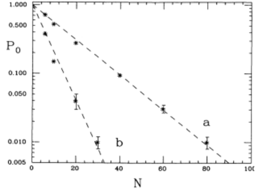
Figure 1: Fraction of maximal Lyapunov exponents smaller than $0.002$ as a function of $N$ for (a) $\varepsilon=0.025$ and (b) $\varepsilon=0.05$, $T=10^{5}$, averaged over $\mathcal{N}=500$ initial conditions.

We start our list of “counter-examples” to the idea that chaotic properties guarantee fast thermalization by recalling the results of FMV91 . In FMV91 the authors studied the ergodic properties of a large number of coupled symplectic maps (1), (2) where one considers periodic boundary conditions, i.e. $\theta_{N+1}=\theta_{1},\,,\,I_{N+1}=I_{1}$, and nearest- neighbour coupling:

$$F(\theta)=\sum_{n=1}^{N}\cos(\theta_{n+1}-\theta_{n})\,.$$

As anticipated above, they find that the volume of phase space filled with invariant manifolds decreases exponentially with system size, as shown in Fig. 1. This is a remarkable evidence that in the large-$N$ limit the probability that thermalization is obstructed by KAM tori is exponentially (in system size) small. The system has good chaotic properties. This notwithstanding, at the same time there are clear signatures of a phenomenon analogous to the so-called weak-ergodicity breaking of disordered systems. The terminology weak-ergodicity breaking is a jargon indicating the situations where, despite relaxation is always achieved asymptotically, at any finite time memory of the initial conditions is preserved CK95 . Let us define as $t_{w}$ the time elapsed since the beginning of the dynamics, $t_{w}+\tau$ is a later time and $C(t_{w},t_{w}+\tau)$ is the time auto-correlation (averaged over an ensemble of initial conditions) of some relevant observable of the system. Weak ergodicity breaking is then expressed by the condition

$$\lim_{\tau\rightarrow\infty}C(t_{w},t_{w}+\tau)=0\quad\quad\quad\quad\quad\forall~{}~{}t_{w}$$

$$C(t_{w},t_{w}+\tau)\neq C(\tilde{t}_{w},\tilde{t}_{w}+\tau)\quad\quad\forall~{}~{}\tau<\infty~{}~{}\&~{}~{}t_{w}\neq\tilde{t}_{w}$$ (10)

A clear signature of a situation with the features of weak ergodicity breaking is revealed by the study of how the distribution of the maximum Lyapunov spectrum depends on the system size FMV91 . While the probability distribution of the exponents peaks at a well defined value at increasing system size, still the scaling of the variance is anomalous, i.e., it has a decay much slower than $1/\sqrt{N}$. One of the main results of FMV91 is that the variance of the Lyapunov exponents distribution, in particular its asymptotic estimate $\sigma_{\infty}(\varepsilon,N)$ scales as

$$\sigma_{\infty}(\epsilon,N)\sim\frac{1}{N^{a(\epsilon)}}$$ (11)

where $a(\epsilon)\sim\sqrt{\epsilon}$, so that for small $\epsilon$, $\sigma_{\infty}(\epsilon,N)$ is much larger that $1/\sqrt{N}$.

III.2 High-temperature features in coupled rotators

Another example of a system which does not show thermal behaviour despite having positive Lyapunov exponents is represented by the coupled rotators at high energy studied in LPRV87 . The Hamiltonian of this system reads as:

$$\mathcal{H}(\bm{\varphi},\bm{\pi})=\sum_{i=1}^{N}\frac{\pi_{i}^{2}}{2}+\varepsilon~{}\sum_{i=1}^{N}(1-\cos(\varphi_{i+1}-\varphi_{i})),$$ (12)

where $\varphi_{i}$ are angular variables and $\pi_{i}$ are their conjugate momenta. The specific heat can be easily computed from the partition function as

$$C_{V} =\frac{\beta^{2}}{N}~{}\frac{\partial^{2}}{\partial\beta^{2}}\log\mathcal{Z}_{N}(\beta).$$ (13)

In particular, the expression of the specific heat reads in term of modified Bessel function as

$$C_{V}=\frac{1}{2}+\beta^{2}\left(1-\frac{1}{\beta}\frac{I_{1}(\varepsilon\beta)}{I_{0}(\varepsilon\beta)}-\left[\frac{I_{1}(\varepsilon\beta)}{I_{0}(\varepsilon\beta)}\right]^{2}\right).$$ (14)

It is possible to compare the analytical prediction of Eq. (14) with numerical simulations by estimating in the latter the specific heat from the fluctuations of energy in a given subsystem of $M$ rotators, with $1\ll M\ll N$:

$$C_{V}=\frac{1}{MT^{2}}\left[\langle\mathcal{H}_{M}^{2}\rangle-\langle\mathcal{H}_{M}\rangle^{2}\right]$$ (15)

where $\mathcal{H}_{M}$ is the Hamiltonian of the chosen subsystem and the “ensemble” average in Eq. (15) includes averaging over initial conditions and averaging along the symplectic dynamics for each initial condition. The result of the comparison is presented in Fig. 2. From the figure it is clear that, while at small and intermediate energies the canonical ensemble prediction for the specific heat matches numerical simulations, it fails at high energies. What is remarkable is that in the high-temperature regime where statistical mechanics fails the value of the largest Lyapunov exponent is even larger that in the intermediate-small energy regime where the equilibrium prediction works well. This is one of the strongest hints from the past literature that the chaoticity of orbits has nothing to do with the foundations of statistical mechanics. In practice it happens that for rotators a sort of “effectively integrable” regime arises at high energy. In this regime each rotator is spinning very fast, something which guarantees the chaoticity of orbits, but the individual degrees of freedom do not interact each other, which causes the breakdown of thermal properties of the system. This very simple mechanism is a concrete example (and often examples are more convincing than arguments) of how absence of thermalization and chaos can be simultaneously present without any problem. With the next example the role of chaos for thermalization will be challenged even further: we are going to present the case of a system which, despite having all Lyapunov exponents equal to zero, relaxes nicely to thermal equilibrium on short time-scales.

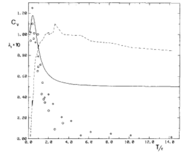
Figure 2: Specific heat versus temperature in the rotator model. The continuous line represents the analytic prediction from Eq. (14). Empty symbols represents the results of numerical simulations, respectively for a subsystem with $M=10$ (circles) and $M=20$ (diamonds) rotators, in a chain of $N=100$ and $N=400$ particles, respectively. The dashed line is the maximal Lyapunov exponent as a function of the temperature (specific energy) measured in units of the coupling constant $\varepsilon$ [see Eq. (12)].

III.3 Toda lattice: thermalization of an integrable system

We present here the example of an integrable system which shows very good thermalization properties. In some sense we find that the statement “the system has thermalized” or “the systems has not thermalized” depends, for Hamiltonian systems, on the choice of canonical coordinates in the same way as the statement “a body is moving” or “a body is at rest” depend on the choice of a reference frame. In this respect, it is true that, if a system is integrable in the sense of the Liouville-Arnol’d theorem and we choose to represent it in terms of the corresponding action-angle variables, we will never observe thermalization. But there are infinitely many other choices of canonical coordinates which allow one to detect a good degree of thermalization. Let us be more specific about this and recall the salient results presented in BVG20 on the Toda chain.

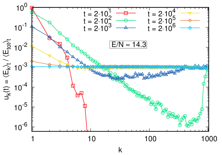
Figure 3: Normalized harmonic energy as a function of the Fourier mode number $k$, for different values of the averaging time, in a Toda dynamics (16) with FPUT initial conditions. Here $N=1023$, total energy $E=14.3$.

It is well known that the Toda lattice

$$\mathcal{H}(q,p)=\sum_{i=1}^{N}\frac{p_{i}^{2}}{2}+\sum_{i=0}^{N}V(q_{i+1}-q_{i}),$$ (16)

where $V(x)$ is the Toda potential

$$V(x)=\exp(-x)+x-1,$$ (17)

admits a complete set of independent integrals of motion, as shown by Henon in his paper H74 . This result can be also understood in the light of Flashka’s proof of the existence of a Lax pair related to the Toda dynamics F74 . The explicit form of such integrals of motion is rather involved, and their physical meaning is not transparent; one may wonder whether the system is able to reach thermalization under a different canonical description, for instance the one which is provided by the Fourier modes

$$Q_{k} =\sum_{i=1}^{N}\frac{\sqrt{2}~{}q_{i}}{\sqrt{N+1}}\sin\left(\frac{\pi ik}{N+1}\right)\,$$

$$P_{k} =\sum_{i=1}^{N}\frac{\sqrt{2}~{}p_{i}}{\sqrt{N+1}}\sin\left(\frac{\pi ik}{N+1}\right)\,.$$ (18)

A typical test which can be performed, inspired by the FPUT numerical experiment, is realized by considering an initial condition in which the first Fourier mode $k=1$ is excited, and $Q_{k}=P_{k}=0$ for all $k>1$; the system is evolved according to its Hamiltonian dynamics, and the average energy corresponding to each normal mode,

$$\langle E_{k}\rangle_{t} =\int_{0}^{t}\left[\frac{P_{k}^{2}}{2}+\omega_{k}^{2}\frac{Q_{k}^{2}}{2}\right]\,dt\,$$

$$\omega_{k} =2\sin\left(\frac{\pi k}{2(N+1)}\right)\,,$$ (19)

is studied as a function of time. It is worth noticing that in the limit of small energy $E$, the Toda Hamiltonian is well approximated by a harmonic chain in which the $P_{k}$’s are conserved quantities; it is therefore not surprising that, for $E/N\ll 1$, it takes very long times to observe equipartition of harmonic energy between the different modes. This ergodicity-breaking phenomenology has been studied, for instance, in Ref. BCP13 to underline relevant similarities with the FPUT dynamics.

The scenario completely changes when specific energies of order $\approx\mathcal{O}(1)$ or larger are considered. In Fig. 3 the distribution of the harmonic energy among the different Fourier modes is shown for several values of the averaging time $t$; no ergodicity breaking can be observed, and in finite times the harmonic energy reaches equipartition.

IV From classical to quantum: open research directions

After the examples of the previous section we feel urged at this point to draw some conclusions. We started our discussion from wondering how much having a phase space uniformly filled by chaotic regions is relevant for relaxation to equilibrium and we came to the conclusion, drawn from the last set of examples, that in practice chaos seems to be at all irrelevant for relaxation to equilibrium. What it is then the correct way to frame the “foundation of statistical mechanics” problem? It seems that the correct paradigm to understand the results of Sec. III is the one established by the ergodic theorem by Khinchin book-K49 : in order to guarantee a thermal behaviour, i.e., that dynamical averages correspond to ensemble averages, it is sufficient to consider appropriate observables for large enough systems. That is, the regime $N\gg 1$ is mandatory. As anticipated in Sec. III by our numerical results, one finds that the hypothesis under which the Khinchin ergodic theorem is valid are for instance fulfilled even by integrable systems. In a nutshell we can summarize his approach saying that it is possible to show the practical validity of the ergodic hypothesis when the following three conditions are fulfilled:

• the number of the degrees of freedom is very large

• we limit the interest to “suitable” observables

• we allow for a failure of the equivalence of the time average and the ensemble average for initial conditions in a “small region”.

The above points will be clarified in the following.

IV.1 The ergodic problem in Khinchin’s perspective

Let us see in practice what the theorem says. Consider a Hamiltonian system $\mathcal{H}({\bf q},{\bf p})$ with canonical variables $({\bf q},{\bf p})=(q_{1},p_{1},\ldots,q_{N},p_{N})$. Let $\Phi_{t}({\bf q},{\bf p})=({\bf q}(t),{\bf p}(t))$ be the flow under the symplectic dynamics generated by $\mathcal{H}({\bf q},{\bf p})$. The time average for given initial datum $x=({\bf q},{\bf p})$ is defined as

$$\overline{f(x)}=\frac{1}{T}\int_{0}^{T}dt~{}f(\Phi_{t}(x))$$ (20)

while the ensemble average is defined with respect to an invariant measure $\mu({\bf q},{\bf p})$ in phase space:

$$\langle f\rangle=\int~{}d\mu({\bf q},{\bf p})~{}f({\bf q},{\bf p}).$$ (21)

Let us define as sum function any function reading as

$$f(x)=\sum_{i=1}^{N}f_{i}({\bf q}_{i},{\bf p}_{i})$$ (22)

For such functions Khinchin book-K49 was able to show that for a random choice of the initial datum $x$ the probability that the time average in Eq. (20) and the ensemble average in Eq. (21) are different is small in $N$, that is:

$$p\left(\left|\frac{\overline{f(x)}-\langle f\rangle}{\langle f\rangle}\right|\geq\frac{C_{1}}{N^{1/4}}\right)<\frac{C_{2}}{N^{1/4}},$$ (23)

where $C_{1}$ and $C_{2}$ are constants with respect to $N$. We can note that many, but not all, relevant macroscopic observables are sum functions. While the original result of Khinchin was for non interacting system, i.e. systems with Hamiltonian

$$\mathcal{H}({\bf q},{\bf p})=\sum_{i=1}^{N}h_{1}(q_{i},p_{i})$$ (24)

Mazur and van der Linden ML63 were able to generalize it to the more physical interesting case of (weakly) interacting particles:

$$H=\sum_{i=1}^{N}h_{1}(q_{i},p_{i})+\sum_{i<j}V(|q_{i}-q_{j}|)$$ (25)

From the results by Khinchin, Mazur and van der Linden we have the following scenario: although the ergodic hypothesis mathematically does not hold, it is “physically” valid if we are tolerant, namely if we accept that in systems with $N\gg 1$ ergodicity can fail in regions sampled with probability of order $O(N^{-1/4})$, i.e. vanishing in the limit $N\to\infty$. Let us stress that the dynamics has a marginal role, while the very relevant ingredient is the large number of particles.

Whereas it is possible, on the one hand, to emphasize some limitations of the Khinchin ergodic theorem, as for instance the fact that it does not tell anything about the timescale to be waited for in order to have Eq. (23) reasonably true, let us stress here its goals. For instance, let us highlight the fact that Khinchin ergodic theorem guarantees the thermalization even of integrable systems! In fact, if we consider the Toda model discussed in the previous section, the conditions under which the Khinchin ergodic theorem was first demonstrated perfectly apply to it. In fact integrability, proved first by Hénon in 1974 H74 , guarantees the existence of $N$ action-angle variables such that the Hamiltonian reads as:

$$\mathcal{H}(\bm{\mathcal{I}},\bm{\phi})=\sum_{i=1}^{N}h_{1}(\mathcal{I}_{i},\phi_{i}),$$ (26)

which is precisely the non-interacting-type of Hamiltonian considered in first instance by Khinchin. The results presented in BVG20 on the fast thermalization of the Toda model has been in fact proposed to re-establish with the support of numerical evidence the assertion, hidden between the lines of the Khinchin theorem and perhaps overlooked so far, that even integrable systems do thermalize in the large-$N$ limit. The phase-space of Toda chain is in fact completely foliated in invariant tori. But, according to Khinchin theorem and our numerical results, this foliation of phase space in regular regions is not an obstacle as long as the “ergodization” of sum functions is considered (for almost all initial data in the limit $N\rightarrow\infty$).

IV.2 Quantum counterpart: Von Neumann’s ergodic theorem

The observation that “even integrable systems thermalize well in the large-$N$ limit” becomes particularly relevant as soon as we regard, in the limit of large $N$, the dynamics of a classical integrable system as the “classical analog” of the dynamics of a quantum system. Indeed in quantum system arises the same “ergodic problem” that we find in classical mechanics, i.e., whether time averages can be replaced by ensemble averages. Let us spend few words on the quantum formalism in order to point out the similarities between the ergodic theorem by Khinchin and the one by Johan Von Neumann for quantum mechanics. As it is well known, due to the self-adjointness of the Hamiltonian operator, any wave vector $|\psi\rangle$ can be expanded on the Hamiltonian eigenvectors basis:

$$|\psi\rangle=\sum_{\alpha\in\text{Sp}(\hat{H})}c_{\alpha}~{}|\alpha\rangle$$ (27)

The projection on a limited set of eigenvalues defines the quantum microcanonical ensemble. Since it is reasonable to assume that also in a quantum system the total energy of an $N$-particles system is known with finite precision, i.e., usually we know that it takes values within a finite shell $\mathcal{I}_{E}\in[E-\delta E,E+\delta E]$ with $E\sim N$ and $\delta E\sim\sqrt{N}$, one defines the microcanonical density matrix as the projector on the eigenstates pertaining to that shell:

$$\hat{\rho}_{E}=\frac{1}{\mathcal{N}_{E}}\sum_{\alpha|\varepsilon_{\alpha}\in\mathcal{I}_{E}}|\alpha\rangle~{}\langle\alpha|,$$ (28)

where $\mathcal{N}_{E}$ is the number of eigenvalues in the shell. The microcanonical expectation of the observable thus read

$$\langle\hat{O}\rangle_{E}~{}=~{}\text{Tr}[\hat{\rho}_{E}\hat{O}]~{}=~{}\frac{1}{\mathcal{N}_{E}}\sum_{\alpha|\varepsilon_{\alpha}\in\mathcal{I}_{E}}\langle\alpha|\hat{O}|\alpha\rangle$$ (29)

Clearly in the limit $N\rightarrow\infty$ where the eigenvalues tend to fill densely the real line one has that even in a finite shell $\mathcal{N}_{E}\sim N$. By preparing a system in the initial state $|\psi_{0}\rangle$ the expectation value of a given observable $\hat{O}$ at time $t$ reads as:

$$\langle\hat{O}(t)\rangle_{\psi_{0}}=\langle\psi_{0}|~{}e^{i\hat{H}t/\hbar}~{}\hat{O}~{}e^{-i\hat{H}t/\hbar}~{}|\psi_{0}\rangle=\langle\psi_{0}(t)|\hat{O}|\psi_{0}(t)\rangle$$

Quantum ergodicity amounts then to the following equivalence between dynamical and ensemble averages,

$$\langle\hat{O}\rangle_{E}~{}=~{}\lim_{T\rightarrow\infty}\frac{1}{T}\int_{0}^{T}dt~{}\langle\hat{O}(t)\rangle_{\psi_{0}}.$$ (31)

The reader can easily convince himself of the fact that, if for almost all times the expectation of $\hat{O}(t)$ on the initial state $|\psi_{0}\rangle$ is typical, namely one has $\langle\hat{O}\rangle_{E}\approx\langle\hat{O}(t)\rangle_{\psi_{0}}$, then the quantum ergodicity property as stated in Eq. (31) is realized. Having for almost all times $\langle\hat{O}\rangle_{E}\approx\langle\hat{O}(t)\rangle_{\psi_{0}}$ is a condition named “normal typicality”: it is discussed thoroughly in GLMTZ10 . Remarkambly in tune with the scenario later proposed by Kinchin for classical system, already in 1929 Von Neumann proposed a quantum ergodic theorem which proves the typicality of $\langle\hat{O}(t)\rangle$ with no references to quantum chaos properties. The definition of quantum chaos, which will be formalized much later BGS84 , is to have a system characterized by a Hamiltonian operator, $\hat{H}|\alpha\rangle=\varepsilon_{\alpha}|\alpha\rangle$, such that its eigenvctors $|\alpha\rangle$ behave as random structureless vectors in any basis. This property, notwidthstanding the different formalism of quantum and classical mechanics, has a deep analogy with the definition of classical chaos casati2006 ; book-CCV09 : a quantum system is said to be chaotic when a small perturbation of the Hamiltonian, $\hat{H}+\hat{\lambda}$ produces totally uncorrelated vectors, $\langle\epsilon_{\alpha}|\epsilon_{\alpha}+\lambda_{\alpha}\rangle\sim 1\/\sqrt{N}$, in the same manned that a small shift in initial conditions produces totally uncorrelated trajectories in classical chaotic systems.
Quite remarkably, Von Neumann’s ergodic theorem does not make any explicit assumption of the above kind on the Hamiltonian’s eigenvalues structure. Here follows a short account of the theorem, mathematical details can be found in the recent translation from German of the original paper JVN10 and in GLMTZ10 ; GLTZ10 . Let $\mathcal{D}$ be the dimensionality of the energy shell $\mathcal{I}_{E}=[E-\delta E,E+\delta E]$, namely $\mathcal{D}=\text{dim}(\mathcal{H}_{E})$ where $\mathcal{H}_{E}$ is the Hilbert space spanned by the eigenvectors $|\alpha\rangle$ such that $\varepsilon_{\alpha}\in\mathcal{I}_{E}$, and define a decomposition of $\mathcal{H}_{E}$ in orthogonal subspaces $\mathcal{H}_{\nu}$ each of dimension $d_{\nu}$:

$$\mathcal{H}_{E}=\bigoplus_{\nu}\mathcal{H}_{\nu}\quad\quad\quad\text{dim}(\mathcal{H}_{\nu})=d_{\nu}\quad\quad\quad\sum_{\nu}d_{\nu}=\mathcal{D}$$ (32)

Then define $\hat{P}_{\nu}$ as the projector on subspace $\mathcal{H}_{\nu}$. It is mandatory to consider the large system size limit where $1\ll d_{\nu}\ll\mathcal{D}$. It is then demonstrated that, under quite generic assumptions on $\hat{H}$ and on the orthogonal decomposition $\mathcal{H}_{E}=\bigoplus_{\nu}\mathcal{H}_{\nu}$, for every wavefunction $|\psi_{0}\rangle\in\mathcal{H}_{E}$ and for almost all times one has normal typicality, i.e.:

$$\langle\psi_{0}|\hat{P}_{\nu}(t)|\psi_{0}\rangle=\text{[}\hat{\rho}_{E}\hat{P}_{\nu}].$$ (33)

A crucial role is played by the assumption that the dimensions $d_{\nu}$ of the orthogonal subspaces of $\mathcal{H}_{E}$ are macroscopically large, i.e. $d_{\nu}\gg 1$. In this sense the projectors $P_{\nu}$ correspond to macroscopic observables. From this point of view the quantum ergodic theorem from Von Neumann is constrained by the same key hypothesis of the Khinchin’s theorem: the limit of a very large number of degrees of freedom. At the same time the Von Neumann theorem does not make any claim on chaotic properties of the eigenspectrum, in the very same way as the Khinchin’s theorem does not make any claim on chaotic properties of trajectories.
For completeness we also need to mention what is regarded nowday as the “modern” version of the Von Neumann theorem, namely the celebrated Eigenstate Thermalization Hypothesis (ETH) RS12 . By expanding the expression of $\langle\hat{O}(t)\rangle_{\psi_{0}}$ as

$$\langle\hat{O}(t)\rangle_{\psi_{0}}=\sum_{\alpha\in\text{Sp}\hat{H}}|c_{\alpha}|^{2}~{}O_{\alpha\alpha}+\sum_{\alpha\neq\beta}e^{i(E_{\alpha}-E_{\beta})t/\hbar}~{}c_{\alpha}^{*}c_{\beta}~{}O_{\alpha\beta}.$$ (34)

it is not difficult to figure out that ergodicity, as expressed in Eq. (31), is guaranteed if suitable hypotheses are made for the matrix elements $O_{\alpha\beta}$. For instance it can be assumed that:

• The off-diagonal matrix elements are exponentially small in system size, $O_{\alpha\neq\beta}\sim e^{-S(E_{0})}$ with $S$ the microcanonical entropy and $E=\langle\psi_{0}|\hat{H}|\psi_{0}\rangle$.

• The diagonal elements are a function of the initial-condition energy, $O_{\alpha\alpha}=O(E_{0})$.

The hypothesis $h.a$ guarantees that for large enough systems relaxation to a stationary state is achieved within reasonable time, still leaving open the possibility that stationarity is different from thermal equilibrium. In fact, it is thanks to the exponentially small size of non-diagonal matrix elements that in the large-$N$ limit one does not need to wait the astronomical times needed for dephasing in order to have

$$\frac{1}{T}\int_{0}^{T}dt~{}\sum_{\alpha\neq\beta}e^{i(E_{\alpha}-E_{\beta})t/\hbar}~{}c_{\alpha}^{*}c_{\beta}~{}O_{\alpha\beta}~{}\approx~{}0$$ (35)

Hypothesis $h.b$ then guarantees that relaxation is towards a state well characterized macroscopically, i.e. a state which depends solely on the energy of the Hilbert space vector $|\psi_{0}\rangle$ and not on the extensive number of coefficients $c_{\alpha}$:

$$\sum_{\alpha\in\text{Sp}\hat{H}}|c_{\alpha}|^{2}~{}O_{\alpha\alpha}=O(E_{0})\cdot\sum_{\alpha\in\text{Sp}\hat{H}}|c_{\alpha}|^{2}=O(E_{0})$$ (36)

Though inspired from the behaviour of (quantum) chaotic systems, ETH is clearly a different property since it makes no claim on the structure of energy eigenvectors. For this reason and also because a necessary condition for ETH to be effective is a large-$N$ limit, ETH is rather close in spirit to the Von Neumann theorem. Then, we must say that a complete understanding of the reciprocal implications of quantum chaos and the Eigenstate Thermalization Hypothesis is still an open issue which deserves further investigations. To this respect let us recall the purpose of this chapter, namely to furnish reasons to believe that an investigation aimed at challenging the role of chaos in the thermalization of both quantum and classical systems is an interesting and timely subject. For instance, a deeper understanding of the mechanisms which triggers, or prevents, thermalization in quantum systems is crucial to estimate the possibilities of having working scalable quantum technologies, like quantum computers and quantum sensors.

An interesting point of view which emerged from the results on the Toda model discussed in Sec. III.3 and which can be traced back to both Khinchin and Von Neumann’s theorem is the following: the presence (or absence) of thermalization is a property pertaining to a given choice of observables and cannot be stated in general, i.e. solely on the basis of the behaviour of trajectories or the structure of energy eigenvectors. We have in mind the choice of the projectors $P_{\nu}$ in Von Neumann theorem and the choice of sum functions in Khinchin theorem. This perspective of considering “thermal equilibrium as a matter of observables choice” is in our opinion a point of view which deserves a careful investigation.

IV.3 Summary and Perspectives

Let us try to summarize the main aspects here discussed. At first we stress that the ergodic approach, even with some caveats, appears the natural way to use probability in a deterministic context. Assuming ergodicity, it is possible to obtain an empirical notion of probability which is an objective property of the trajectory. An important aspect often non considered is that both in experiments and numerical computation one deals with a unique system with many degrees of freedom, and not with an ensemble of systems. According to the point of view of Boltzmann (and the developments by Khinchin, Mazur and van der Linden) it is rather natural to conclude that, at the conceptual level, the only physically consistent way to accumulate a statistics is in terms of time averages following the time evolution of the system. At the same time ergodicity is a very demanding property and, since in its definition it requires to consider the infinite time limit, physically it is not very accessible.

We have then presented a strong evince from numerical study of high dimensional Hamiltonian systems that chaos is neither a necessary nor a sufficient ingredient to guarantee the validity of equilibrium statistical mechanics for classical systems. On the other hand, even when chaos is very weak (or absent), we have shown examples of a good agreement between time and ensemble averages BVG20 . The perspective emerging from our study is that the choice of variables is thus a key point to say whether a system has thermalized or not. We have found that this point of view emphasizes the commonalities between classical and quantum mechanics for what concerns the ergodic problem. This is particularly clear by comparing the assumptions and the conclusions of the ergodic theorems of Khinchin and Von Neumann, where, without any assumption on the chaotic nature of dynamics, it is shown that for general enough observables a system has good ergodic properties even in the case where interactions are absent, provided that the system is large enough.

This brought us to underline as a possibly relevant research line the one dedicated to find “classical analogs” of thermalization problems in quantum systems and to study such problems with the conceptual tools and the numerical techniques developed for classical Hamiltonian systems.

The ability to control and exactly predict the behavior of quantum systems is in fact of extreme relevance, in particular for the great bet presently made by the worldwide scientific community on quantum computers. In particular, understanding the mechanisms preventing thermalization might certainly help to improve the function of quantum processors and to devise better quantum algorithms.

In summary, we tried to present conving motivations in favour of a renewed interest towards the foundations of quantum and statistical mechanics. This is something which in our opinion is worth to be pursued while approaching the one century anniversary of the two seminal papers of Heisenberg He25 and Schrödinger Sch26 on quantum mechanics. How much the quantum mechanics revolution has influenced across one hundred year not only the understanding of the microscopic world but even the thermodynamic properties of macroscopic systems? This the, still actual, key question of our reserch line.

- (1) T. D. Lee, “Particle Physics and Introduction to Field Theory”, Harwood Academic Publishers, New York (1981).
- (2) P. Castiglione, M. Falcioni, A. Lesne and A. Vulpiani, “Chaos and Coarse Graining in Statistical Mechanics” (Cambridge University Press, 2008).
- (3) M. Cencini, F. Cecconi and A. Vulpiani, “Chaos: From Simple Models to Complex Systems” (World Scientific, Singapore, 2009).
- (4) Y. Oono, “The Nonlinear World” (Springer Verlag, (2013).
- (5) A. I. Khinchin, “Mathematical Foundations of Statistical Mechanics” (Dover, 1949).
- (6) J. Von Neumann ,“Proof of the Ergodic Theorem and H-Theorem in Quantum Mechanics”, EPJ H 35, 201 (2010).
- (7) S. Goldstein, J. L. Lebowitz, C. Mastrodonato, R. Tumulka, N. Zanghì, “Normal typicality and von Neumann’s quantum ergodic theorem”, Proc. R. Soc. A. 466, 3203–3224 (2010).
- (8) S. Goldstein, J. L. Lebowitz, R. Tumulka, N. Zanghí, “Long-time behavior of macroscopic quantum systems”, EPJ H 35, 173 (2010).
- (9) G. Emch and C. Liu “The Logic of Thermo-Statistical Physics” (Springer Verlag, (2002).
- (10) G. Gallavotti (Ed.) “The Fermi-Pasta-Ulam problem: a status report” (Springer, 2008).
- (11) G. Benettin, H. Chrisodoulidi, A. Ponno, “The Fermi-Pasta-Ulam Problem and Its Underlying Integrable Dynamics”, J. Stat. Phys. 152, 195–212 (2013).
- (12) A. Pikovsky and A. Politi, “Lyapunov Exponents, A Tool to Explore Complex Dynamics” (Cambridge University Press, 2016).
- (13) K. Kaneko and R. J. Bagley, “Arnold diffusion, ergodicity and intermittency in a coupled standard mapping”, Phys. Lett. A 110, 435 (1985).
- (14) M. Falcioni, U. Marini Bettolo Marconi, A. Vulpiani, “Ergodic properties of high-dimensional symplectic maps”, Phys. Rev. A 44, 2263 (1991).
- (15) J. F. Yamagishi and K. Kaneko, “Chaos with a high-dimensional torus”, Phys. Rev. Res. 2, 023044 (2020).
- (16) L. Hurd, C. Grebogi and E. Ott, “On the tendency toward ergodicity with increasing number of degrees of fredom in Hamiltonian systems”, in J. Siemenis (ed.), Hamiltonian Mechanics, p. 123 (Plenum, New York, 1994).
- (17) M. Mézard, G. Parisi, M.-A. Virasoro, “Spin Glass theory and beyod” (World Scientific, 1987).
- (18) K. Kaneko and T. Konishi, “Transition, Ergodicity and Lyapunov Spectra of Hamiltonian Dynamical Systems”, J. of Phys. Soc. of Japan 56, 2993 (1987).
- (19) R. Livi, A. Politi and S. Ruffo, “Distribution of characteristic exponents in the thermodynamic limit”, J. Phys. A: Math. Gen. 19, 2033 (1986).
- (20) L. A. Bunimovich and G. Sinai “Statistical mechanics of coupled map lattices”, in Theory and Applications of Coupled Map Lattices, ed. K. Kaneko, p. 169 (New York: Wiley 1993).
- (21) R. Livi, M. Pettini, S. Ruffo, A. Vulpiani, “Chaotic Behavior in Nonlinear Hamiltonian Systems and Equilibrium Statistical Mechanics”, J. Stat. Phys. 48, 539 (1987).
- (22) M. Hénon, “Integrals of the Toda lattice”, Phys. Rev. B 9, 1921 (1974).
- (23) L. F. Cugliandolo, J. Kurchan, “Weak ergodicity breaking in mean-field spin-glass models”, Philosophical Magazine B 71, 501-514 (1995).
- (24) M. Baldovin, A. Vulpiani, G. Gradenigo, “Statistical mechanics of an integrable system”, J Stat Phys 183, 41 (2021).
- (25) H. Flaschka, “The Toda lattice. II. Existence of integrals”, Phys. Rev. B 9, 1924–1925 (1974).
- (26) P. Mazur, J. van der Linden, “Asymptotic form of the structure function for real systems” J. Math. Phys. 4, 271 (1963).
- (27) O. Bohigas, M. Giannoni, C. Schmit, “Characterization of Chaotic Quantum Spectraand Universality of Level Fluctuations Law”, Phys. Rev. Lett. 52 (1984).
- (28) G. Casati, B. Chirikov (Eds.), “Quantum chaos: between order and disorder” Cambridge University Press (2006).
- (29) M. Rigol, M. Srednicki, “Alternatives to Eigenstate Thermalization”, Phys. Rev. Lett. 108, 110601 (2012).
- (30) W. Heisenberg, “Über quantentheoretische Umdeutung kinematischer undmechanischer Beziehungen”, Z. Phys. 33, 879 (1925).
- (31) E. Schrödinger, “An ondulatory theory of the mechanics of atoms and molecules”, Phys. Rev. 28, 1049 (1926).