Cosmology with Love: Measuring the Hubble constant using neutron star universal relations

Abstract

Gravitational-wave cosmology began in 2017 with the observation of the gravitational waves emitted in the merger of two neutron stars, and the coincident observation of the electromagnetic emission that followed. Although only a $30\%$ measurement of the Hubble constant was achieved, future observations may yield more precise measurements either through other coincident events or through cross correlation of gravitational-wave events with galaxy catalogs. Here, we implement a new way to measure the Hubble constant without an electromagnetic counterpart and through the use of the binary Love relations. These relations govern the tidal deformabilities of neutron stars in an equation-of-state insensitive way. Importantly, the Love relations depend on the component masses of the binary in the source frame. Since the gravitational-wave phase and amplitude depend on the chirp mass in the observer (and hence redshifted) frame, one can in principle combine the binary Love relations with the gravitational-wave data to directly measure the redshift, and thereby infer the value of the Hubble constant. We implement this approach in both real and synthetic data through a Bayesian parameter estimation study in a range of observing scenarios. We find that for the LIGO/Virgo/KAGRA design sensitivity era, this method results in a similar measurement accuracy of the Hubble constant to those of current-day, dark-siren measurements. For third generation detectors, this accuracy improves to $\lesssim 10\%$ when combining measurements from binary neutron star events in the LIGO Voyager era, and to $\lesssim 2\%$ in the Cosmic Explorer era.

I Introduction

The inference of cosmological parameters like the Hubble constant, $H_{0}$, using gravitational waves (GWs) hinges on the standard siren approach [1, 2]. The central idea is to measure the luminosity distance, $D_{L}$, from the GW data while simultaneously identifying an electromagnetic (EM) signal from the source. The independent measurement of $D_{L}$ and the cosmological redshift, $z$, leads to a measurement of $H_{0}$. In the absence of a counterpart, clustering of $H_{0}$ measurements from potential host galaxies for a large sample of events also leads to a statistical measurement of $H_{0}$ [3]. This idea found its first application in the simultaneous panchromatic observations of GWs, gamma-rays, optical, and infrared radiation from the binary neutron star (BNS) merger seen by the Advanced Laser Interferometer Gravitational-wave Observatory (LIGO) [4] and Advanced Virgo [5] detectors, GW170817 [6]. The identification of the host galaxy, NGC 4993, led to an independent measurement of $H_{0}$ [7]. Also, the $\sim 16{\text{deg}^{2}}$ sky-localization led to a statistical measurement of $H_{0}$, agnostic of the host galaxy information [8]. Such independent measurements are crucial in the light of the recent tension in the value of $H_{0}$ measured from observations of the early and late-time universe [9].

A different approach of estimating the distance-redshift relation, solely using GWs from merging BNS systems, was first proposed by Messenger and Read [10]. Measuring the redshift is challenging because while the amplitude of the GW encodes information about $D_{L}$, the mass parameters are degenerate with the redshift, resulting in the measurement of the redshifted mass at the detector as opposed to the true source-frame mass, i.e., $m_{\text{det}}=(1+z)m_{\text{source}}$. However, matter effects in BNS inspirals, characterized by the tidal deformability parameter, $\bar{\lambda}$, breaks this degeneracy since the tidal deformability is a function of the source-frame mass, $m_{\text{source}}$. This feature has been exploited in the literature via an expansion of $\bar{\lambda}$ in terms of $m_{\text{source}}$ [11, 12, 13]. However, the expansion coefficients are dependent on the NS equation of state (EoS), which is uncertain. This implies that, in the absence of a priori information about the EoS, the expansion coefficients are free parameters in data analysis, and an extraction of the $H_{0}$ is difficult.

This degeneracy, however, can be broken through a set of universal relations discovered by Yagi and Yunes [14, 15] (hereafter YY17). Their work has shown that there exists tight relations between these expansion coefficients that are insensitive to the EoS. Using these so called $\bar{\lambda}^{(0)}_{0}-\bar{\lambda}^{(k)}_{0}$ binary Love relations, knowing one of the expansion coefficient (which we call $\bar{\lambda}^{(0)}_{0}$) determines the others, and this reduces the number of free parameters drastically. Since the $\bar{\lambda}^{(0)}_{0}$ is universal, the measurements can be stacked using data from gold-plated BNS events for which the source frame mass, or equivalently the redshift, is known. Subsequently, its value may be fixed to express $\bar{\lambda}=\bar{\lambda}(m_{\text{source}})$ for future BNS detections leading to a measurement of $m_{\text{source}}$, or equivalently the redshift, and thus $H_{0}$.

In this paper, we use the YY17 prescription to construct a $\bar{\lambda}^{(0)}_{0}-\bar{\lambda}^{(k)}_{0}$ relation using EoSs that satisfy the current constraint on mass and radii of NSs from LIGO/Virgo for GW170817 [16] and the same from by the Neutron Star Interior Composition Explorer (NICER) measurements of the millisecond pulsar, PSR J0030+0451 [17]. We then perform Bayesian parameter estimation on GW170817 data, employing this relation to measure the free coefficient, $\bar{\lambda}^{(0)}_{0}$, appearing in the expansion. We then analyze the prospects of measuring $H_{0}$ by performing Bayesian parameter estimation on a set of simulated (synthetic) BNS signals across different detector eras. While the $H_{0}$ measurement from individual events may not be very constraining due to the distance-inclination degeneracy in GW parameter estimation, we show that by combining the result from multiple events, the stacked measurement of $H_{0}$ converges to the true value. We find that for the design sensitivity LIGO/Virgo/KAGRA/India (HLVKI) era, the measurement accuracy is comparable to the current dark siren measurements [18, 19], or from recent counterpart measurement, assuming the association of GW190521 and ZTF19abanrhr, [20, 21] shown in Refs. [22, 23]. This accuracy improves to $\sim 10\%$ in the Voyager era assuming $\mathcal{O}(10^{2})$ BNS events, and to $\sim 2\%$ for $\mathcal{O}(10^{3})$ detections in the Cosmic Explorer (CE) era. Ultimately, the accuracy of the measurement of $H_{0}$ will be limited by systematic uncertainties in the binary Love method, and we study what limits these systematic uncertainties place on future measurements of $H_{0}$.

The organization of this paper is as follows. In Sec. II, we summarize the universal binary love relations in brief. We show the construction of the $\bar{\lambda}^{(0)}_{0}-\bar{\lambda}^{(k)}_{0}$ relation for this work. In Sec. III, we show our measurement for $\bar{\lambda}^{(0)}_{0}$ by performing Bayesian parameter estimation on GW170817 data. In Sec. IV, we use the results of $\bar{\lambda}^{(0)}_{0}$ and simulated BNS events across different generations of ground-based detectors to show the prospects of measuring $H_{0}$ using multiple events. In Sec. V, we consider the systematic errors that could arise in the measurement of $H_{0}$ due to uncertainty in measurement of $\bar{\lambda}^{(0)}_{0}$, and from uncertainties in the $\bar{\lambda}^{(0)}_{0}-\bar{\lambda}^{(k)}_{0}$ relations. Finally, we conclude in Sec. VI. We follow the conventions of Ref. [24], and when necessary, use geometric units $G=1=c$.

II Binary Love Relations

The quasi-circular inspiral of a compact binary system is described under the post-Newtonian (PN) formalism [25], where the system parameters, like masses and spins, appear in the coefficients of the expansion at different PN orders. While the GW signal from a BNS system has similar morphology to an analogous binary black hole (BBH) system during the early inspiral phase, strong gravitational effects in the late inspiral stage deforms the NSs, leading to additional multipolar deformations that enhances GW emission and leads to an earlier merger [26]. The deformation of the NS is characterized by the electric-type, $\ell=2$, tidal deformability parameter, $\bar{\lambda}=(2k_{2}/3)C^{-5}$, where $C=M/R$ is the compactness of a NS with mass $M$ and radius $R$, which therefore depends on the EoS, and $k_{2}$ is the relativistic Love number [27]. This tidal deformation modifies the binding energy of the binary, which in turn modifies the chirping rate, and therefore the waveform phase, with finite-size effect appearing first at 5PN order  [26]. In a BNS system, the waveform phase will have modifications that will depend on the tidal deformability of each binary component, but there exist certain EoS-insensitive relations that relate them. We present them here in brief, and refer the interested reader to YY17 for further details (see also [28] for a similar EoS-insensitive relation between the tidal deformability of each component).

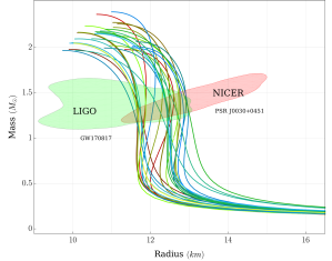
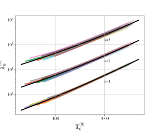
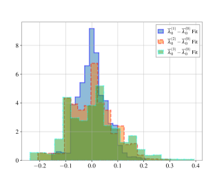
Figure 1: Upper panel: Mass-radius relations for 29 piecewise polytropic EoSs that are consistent with the LIGO/Virgo and NICER observations to 68% confidence. Middle panel: $\bar{\lambda}^{(k)}_{0}=\bar{\lambda}^{(k)}_{0}(\bar{\lambda}^{(0)}_{0})$ relations for the same set of EoSs, together with the fit in thick lines. Observe that the $\bar{\lambda}^{(0)}_{0}-\bar{\lambda}^{(k)}_{0}$ relations are EoS insensitive and the fit recovers the average. Bottom panel: Distribution of the fractional residual errors from the fit for each coefficient.

While the internal composition of NSs is extremely complex, certain relations among some observables, like the moment of inertia, the quadrupole moment, and the tidal deformability, are insensitive to the details of the microphysics [29, 30] (see Refs. [31, 32] for reviews on universal relations). In the context of GW astrophysics, these imply certain binary Love relations, presented in YY17:

1. A relation between the symmetric and anti-symmetric combination of the individual tidal deformabilities, $\bar{\lambda}_{s}=(\bar{\lambda}_{1}+\bar{\lambda}_{2})/2$ and $\bar{\lambda}_{a}=(\bar{\lambda}_{1}-\bar{\lambda}_{2})/2$.

2. A relation between the waveform tidal parameters $\bar{\Lambda}$ and $\delta\bar{\Lambda}$ appearing in 5-PN and 6-PN order respectively.

3. A relation between the coefficients of the Taylor expansion of the tidal deformability $\bar{\lambda}(M)$ about some mass $m_{0}$ as a function of mass.

Here, we are concerned with the third item in this list, and we will refer to it as the $\bar{\lambda}^{(0)}_{0}-\bar{\lambda}^{(k)}_{0}$ relation.

The central idea of the $\bar{\lambda}^{(0)}_{0}-\bar{\lambda}^{(k)}_{0}$ relation is to express $\bar{\lambda}(M)$ in terms of a Taylor expansion about a fiducial value, $M=m_{0}$ as,

$$\bar{\lambda}(M)=\sum_{k=0}^{\infty}\frac{\bar{\lambda}^{(k)}_{0}}{k!}\left(1-\frac{M}{m_{0}}\right)^{k},$$ (1)

where, $\bar{\lambda}^{(k)}_{0}=(-1)^{k}d^{k}\bar{\lambda}/{dM^{k}}$ is evaluated at $M=m_{0}$. The $\bar{\lambda}^{(0)}_{0}-\bar{\lambda}^{(k)}_{0}$ relation states that $\bar{\lambda}^{(k)}_{0}$ can be written entirely in terms of $\bar{\lambda}^{(0)}_{0}$, and the resulting expression is insensitive to the EoS. (to fractional accuracy of about $10\%$).

The $\bar{\lambda}^{(0)}_{0}-\bar{\lambda}^{(k)}_{0}$ relation can be evaluated for any tabulated EoS, but as a Fermi estimate, we first consider the simplified example of a polytropic EoS. For such an EoS, the pressure ($p$) and energy density ($\epsilon$) are related via $p\propto\epsilon^{1+1/n}$, where $n$ is the polytropic index. To leading order in compactness, the tidal deformability is then given by [30], $\bar{\lambda}\propto M^{-10/(3-n)}$. The $\bar{\lambda}^{(0)}_{0}-\bar{\lambda}^{(k)}_{0}$ relation in this case then becomes, $\bar{\lambda}^{(k)}_{0}=G_{n,k}\bar{\lambda}^{(0)}_{0}$, where we have defined

$$G_{n,k}=\frac{\Gamma\left(k+\frac{10}{3-n}\right)}{\Gamma\left(\frac{10}{3-n}\right)}.$$ (2)

Thus, the binary-love-relations ensure that $\bar{\lambda}^{(k)}_{0}=\bar{\lambda}^{(k)}_{0}(\bar{\lambda}_{0}^{(0)})$ for $k>1$, with the relation only dependent on $n$.

In the relativistic case and for more realistic EoSs, the tidal deformability is obtained numerically, and the $\bar{\lambda}^{(0)}_{0}-\bar{\lambda}^{(k)}_{0}$ relation is obtained by fitting the numerical simulations to an expression of the form (see Eq. (22) of YY17),

$$\bar{\lambda}^{(k)}_{0}=G_{\bar{n},k}\;\bar{\lambda}^{(0)}_{0}\left(1+\sum_{i=1}^{3}a_{i,k}x^{i}\right),$$ (3)

where $x=(\bar{\lambda}^{(0)}_{0})^{1/5}$, $a_{i,k}$ are numerical coefficients, and $G_{\bar{n},k}$ is defined in Eq. (2). Here, we will only consider an expansion to $k=3$. This is sufficient to accurately represent $\bar{\lambda}(M)$ in the range $M\in(1.2M_{\odot},1.5M_{\odot})$ for $m_{0}=1.4M_{\odot}$, which we will choose for the rest of this work. The degree of universality deteriorates as $k$ increases, but the overall sum is still EoS insensitive to about $10\%$ for the mass range and $m_{0}$ mentioned.

k	1	2	3
$a_{1,k}$	$-0.349$	$-1.063$	$-1.820$
$a_{2,k}$	5.674	10.649	14.693
$a_{3,k}$	0.296	1.800	2.741

Table 1: Coefficients found by fitting the function in Eq. (3) to the $\bar{\lambda}^{(k)}_{0}-\bar{\lambda}^{(0)}_{0}$ relation data calculated from the 29 EoSs we considered in this work. See middle (lower) panel of Fig. 1 for the fit (residuals).

We re-derive the fitting coefficients $a_{i,k}$ for a set of EoSs that are consistent with recent LIGO/Virgo and NICER observations (and the observation of $\sim 2M_{\odot}$ neutron stars [33, 34, 35]). For simplicity, we here consider the piecewise polytropic representation of the EoS [36], restricting attention only to those that have support in the $68\%$ confidence region in terms of mass and radii reported by LIGO/Virgo in Ref. [16], and NICER in Ref. [17]. The upper and middle panels of Fig. 1 show the mass-radius curves and the $\bar{\lambda}^{(0)}_{0}-\bar{\lambda}^{(k)}_{0}$ relation constructed with the 29 EoSs used in this work. Using Eq. (3) to fit for the $a_{i,k}$ coefficients up to $k=3$ yields the coefficients listed in Table II. These fitting functions give us an EoS averaged $\bar{\lambda}^{(0)}_{0}-\bar{\lambda}^{(k)}_{0}$ relation, as one can see from the middle panel of Fig. 1. Note that $\bar{\lambda}^{(0)}_{0}$ is still a free parameter that is to be constrained by observational data. We will here use this fit to parameterize the tidal deformability and perform Bayesian parameter estimation on GW170817 data to measure the constant $\bar{\lambda}^{(0)}_{0}$.

III $\bar{\lambda}^{(0)}_{0}$ from GW170817

The first step in estimating the Hubble parameter with the binary Love relations is to estimate $\bar{\lambda}^{(0)}_{0}$ with a controlled event. We provide a brief review of Bayesian inference. The aim of Bayesian inference is to obtain a posterior probability density for the parameters describing the signal, $\boldsymbol{\Theta}$, given the GW data, $d^{\text{GW}}$,

$$p(\boldsymbol{\Theta}|d^{\text{GW}})\propto p(d^{\text{GW}}|\boldsymbol{\Theta})\;p(\boldsymbol{\Theta}).$$ (4)

Here, $p(d^{\text{GW}}|\boldsymbol{\Theta})$ is the likelihood of the parameters and $p(\boldsymbol{\Theta})$ is the prior distribution. Gravitational waves from compact binary coalescences of BBHs are described by 15 parameters. These contain the intrinsic parameters like the masses ($m_{1,2}$) and spin parameter 3-vectors ($\boldsymbol{a}_{1,2}$), and the extrinsic parameters like luminosity distance, $D_{L}$, inclination angle, $\iota$, and so on (see, for example, Refs. [37, 38, 39, 40, 41]). In the case of BNSs, matter effects enter the waveform phase first at 5PN and then 6PN order via two additional tidal deformability parameters, $\bar{\lambda}_{1,2}$, as,

$$\Psi_{\text{tid}} = -\frac{3}{128\eta x^{5/2}}\left[\frac{39}{2}\bar{\Lambda}x^{5}+\right.$$ (5)

$$\left.\left(\frac{3115}{64}\bar{\Lambda}-\frac{6595}{364}\sqrt{1-4\eta}\delta\bar{\Lambda}\right)x^{6}+\mathcal{O}(x^{7})\right],$$

where $x=\left[\pi(m_{1}+m_{2})f\right]^{2/3}$ is the PN expansion parameter, $f$ is the GW frequency, and $\eta=m_{1}m_{2}/(m_{1}+m_{2})^{2}$ is the symmetric mass-ratio. The expressions for $\bar{\Lambda}$ and $\delta\bar{\Lambda}$ have the form,

$$\bar{\Lambda} = f(\eta)\left(\frac{\bar{\lambda}_{1}+\bar{\lambda}_{2}}{2}\right)+g(\eta)\left(\frac{\bar{\lambda}_{1}-\bar{\lambda}_{2}}{2}\right)$$

$$\delta\bar{\Lambda} = \delta f(\eta)\left(\frac{\bar{\lambda}_{1}+\bar{\lambda}_{2}}{2}\right)+\delta g(\eta)\left(\frac{\bar{\lambda}_{1}-\bar{\lambda}_{2}}{2}\right),$$ (6)

where the exact expressions for $\{f,g,\delta f,\delta g\}$ are given in Sec. 2.2 of YY17. In our case, we are interested in measuring the tidal deformability by using the parameterization described in Eq. (1) and Eq. (3), but of course, all waveform parameters must be searched over when exploring the likelihood surface.

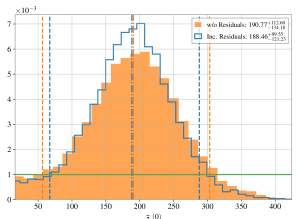
Figure 2: Posterior probability density for the $\bar{\lambda}^{(0)}_{0}$ parameter measured from 128s of strain data (4 kHz) for GW170817. The $\bar{\lambda}^{(0)}_{0}-\bar{\lambda}^{(k)}_{0}$ relations are used in the parameterization of the tidal deformability in Eq. (1) with (unfilled) and without (filled) the residual errors in the relations. The redshift is fixed at the host galaxy $z_{\text{NGC4993}}=0.0099$, and therefore, the tidal deformability is parameterized only by $\bar{\lambda}^{(0)}_{0}$. The vertical dash-dot lines represent the median, the vertical dashed lines represent the 90% confidence interval, and the horizontal line is the prior density.

To obtain a measurement for $\bar{\lambda}^{(0)}_{0}$, we perform Bayesian parameter estimation on 128s of 4 kHz strain data for GW170817. For the model, we use the IMRPhenomPv2_NRTidal waveform [42], which is the same as that used for parameter estimation in Ref. [43] and Ref. [44] (hereafter LV19). In our analysis, however, the parameters $\bar{\lambda}_{1,2}$ are not independent, but rather they are modeled through the Taylor expansion in Eq. (1), with the EoS-insensitive $\bar{\lambda}^{(0)}_{0}-\bar{\lambda}^{(k)}_{0}$ relation of Eq. (3). This then means that $(\bar{\Lambda},\delta\bar{\Lambda})$ (or equivalently $(\bar{\lambda}_{1},\bar{\lambda}_{2})$) are not parameters of our model anymore, but rather the model now only depends on a single tidal deformability parameter, namely $\bar{\lambda}^{(0)}_{0}$. The model also depends on the detector-frame masses ${m_{\text{det}}}{}_{1,2}$ and the redshift $z$, since the Taylor expansion of Eq. (1) depends on the source-frame masses ${m_{\text{source}}}{}_{1,2}$. For the GW170817 event, however, the redshift is known to high accuracy due to identification of the host galaxy, and so this is no longer a free parameter in this case.

The priors on the parameters of our model are chosen as follows. For the extrinsic parameters, like the distance, inclination, coalescence phase, sky-position and so on we pick uninformative priors as those in LV19. Following LV19, we sample on detector-frame component masses setting the prior distribution of each component mass as the marginalized posterior distribution obtained for the component masses from LV19. We also repeat the analysis putting a flat prior on the component masses as in LV19, and find similar results. For the spins, we use the low-spin prior from LV19 i.e., $\chi_{i}\leq 0.05$. For $\bar{\lambda}^{(0)}_{0}$, we use a flat prior in $[0,1000]$, which implies a prior on the individual tidal deformabilities through Eq. (1) for a fixed redshift. The implied priors on the individual tidal deformabilities are shown in Appendix A. This step is different from LV19, where a uniform prior was used on the individual tidal deformabilities, $\bar{\lambda}_{1,2}$, independently. We fix the redshift of the source at the value of the host galaxy NGC4993, $z_{\text{NGC4993}}=0.0099$, which was determined through EM observations reported in Ref. [45], and used in LV19. This allows us to obtain the source-frame component masses, ${m_{\text{source}}}_{1,2}={m_{\text{det}}}_{1,2}/(1+z_{\text{NGC4993}})$. The setup of the likelihood function and the sampling is done through the open-source GW parameter estimation library, BILBY, [46] using with the adaptive nested sampler, DYNESTY [47]. The resulting marginalized distribution for $\bar{\lambda}^{(0)}_{0}$ is shown in Fig. 2. The distribution of the other parameters is presented in Appendix B.

We find the value of $\bar{\lambda}^{(0)}_{0}=191^{+113}_{-134}$ at 90% confidence. In order to verify the measurement is robust against the residual errors coming from the $\bar{\lambda}^{(0)}_{0}-\bar{\lambda}^{(k)}_{0}$ relation fit, we repeat the analysis sampling in $\bar{\lambda}^{(0)}_{0}$, but also sampling from the residual error in the $\bar{\lambda}^{(k)}_{0}(\bar{\lambda}^{(0)}_{0})$ relation error, shown in the bottom panel of Fig. 1. In this case, when sampling, for each throw of a $\bar{\lambda}^{(0)}_{0}$ sample, we obtain the $\bar{\lambda}^{(k)}_{0}$ using the fit and a sample from the distribution of residuals. The posterior density of $\bar{\lambda}^{(0)}_{0}$ obtained this way is shown in Fig. 2 using the un-filled histogram. We find that the result is not significantly affected ($\sim 2\%$ difference in median values). Our results are consistent with the measurement of $\bar{\lambda}(1.4M_{\odot})=190^{+390}_{-120}$ obtained by a linear expansion of $\bar{\lambda}(m_{\text{source}})m_{\text{source}}^{5}$ about $1.4~{}M_{\odot}$, reported in Ref. [16] following the approach in Refs. [12, 13]. The difference in the upper limit is caused due to differences in prior implied on the tidal deformabilities. In Appendix A, we compare our prior with that in Ref. [16].

The first measurement of $\bar{\lambda}^{(0)}_{0}$ reported above is perhaps not extremely constraining, but one expects future events to allow for more accurate measurements. Future observing runs of LIGO/Virgo/KAGRA with coincident operation of next generation telescope facilities, like the Rubin Observatory [48], will yield many more multi-messenger BNS events. We can think of $\bar{\lambda}^{(0)}_{0}$ as a variable which parameterises $\bar{\lambda}$ as a function of the source mass as in Eq. (1). Using the parameterization in Eq. (1) we can stack data from multiple observations to yield an improved measurement of $\bar{\lambda}^{(0)}_{0}$. This implies that eventually, we will be able to “fix” the value of $\bar{\lambda}^{(0)}_{0}$, or marginalize over the small measurement (and eventually systematic) uncertainties.

IV Measuring $H_{0}$ with Love

If $\bar{\lambda}^{(0)}_{0}$ has been estimated by a set of controlled observations (like the GW170817 event), what else can be done with additional future observations of BNS events? Using the same parameterization in Eq. (1), we see then that the tidal deformability terms of the waveform phase are now only a function of $m_{\text{source}}$, or equivalently of the detector-frame masses and the redshift. Since the detector-frame masses can be separately and tightly estimated from lower-PN order terms, the tidal deformability terms now yield information exclusively on the redshift [10]. Therefore, any BNS signal, irrespective of being well-localized or having an associated counterpart, would result in a direct measurement of the redshift from the tidal deformability, and this can be used to infer the Hubble constant, $H_{0}$.

Let us then consider the prospects of measuring $H_{0}$ with future observations, beginning with a best-case scenario, in which we assume $\bar{\lambda}^{(0)}_{0}$ has been strongly constrained. We re-write Eq. (1) as,

$$\bar{\lambda}_{1,2}=\bar{\lambda}^{(0)}_{0}+\sum_{k=1}^{N}\frac{\bar{\lambda}^{(k)}_{0}}{k!}\left(1-\frac{m_{\text{det}}{}_{1,2}/m_{0}}{1+z(D_{L},H_{0},\mathbf{\Omega})}\right)^{k},$$ (7)

where $\mathbf{\Omega}=\{\Omega_{i}\}$ are the cosmological parameters apart from $H_{0}$, which we here, for simplicity, fix to a flat $\Lambda\text{CDM}$ model with an assumed “true” value of $H_{0}$= 70 $\text{km s}^{-1}/\text{Mpc}$ and matter-to-critical-density ratio $\Omega_{m0}=0.3$. Hence, we can write $z=z(D_{L},H_{0})$ in Eq. (7). The measurement of $D_{L}$ comes from the waveform amplitude, and thus the redshift, $z$, alone comes from Eq. (7). This enables either direct sampling of $H_{0}$, or we can infer $H_{0}$ in a post-processing step after we have sampled in $z$.

Even though the logic behind this idea is straightforward and robust, its implementation for a single event is hindered by measurement uncertainties and covariances. In particular, the distance-inclination degeneracy in the amplitude implies that distance measurements peak at lower-than-true values for face-on sources, and to greater-than-true values for edge-on sources (see Refs. [3, 49], for example). Thus, $H_{0}$ measurements from individual events may be multi-modal and, in general, peaked away from the true value. However, since all observations should depend on the same $H_{0}$ (assuming this quantity is truly a constant), one should be able to stack multiple events to obtain an accurate measurement of the Hubble constant.

Figure 3: Left: Individual (dotted) and stacked (solid) $H_{0}$ likelihoods obtained for the representative runs in the O5 (top), Voyager (middle) and CE (bottom) observing eras. Due to distance-inclination degeneracy, the individual posteriors are sometimes peaked away from the true value. However, after stacking the posteriors based on a sample of $N_{\text{det}}$ events from the detected population, the distribution converges to the true simulated value, shown by the vertical line, $H_{0}=70\text{km s}^{-1}/\text{Mpc}$. For illustration, we choose $N_{\text{det}}$=10, 50, 70 for the top middle, and bottom panels, corresponding to the O5, Voyager, and CE era, respectively. Right: The normalized number count of of distances and inclinations of the systems that would be detectable in a specific observing era is shown by the contour map. This was obtained by simulating an ensemble (several thousands) of binaries with $(m_{1},m_{2})\sim(1.42,1.27)~{}M_{\odot}$ distribution uniform in sky, volume, and inclination, and requiring that each produce network SNR $\geq 8$. The grid of overlayed points represents the true distance/inclination of synthetic systems chosen for performing Bayesian parameter estimation. We observe that the $H_{0}$ measurement converges irrespective of the shape of grid as long as it covers the distances and inclinations that would be detected.

We investigate how this stacking measurement could take place in the future. We simulate synthetic GW signals in three different networks of detectors: ground-based observatories in the O5 era (HLVKI 5 detector network), the Voyager era (HLI upgraded to Voyager + VK), and the Cosmic Explorer era (1 CE instrument at H). For simplicity, we consider a set of BNS signals produced by systems with a fixed source frame chirp mass, $\mathcal{M}_{c}=1.17~{}M_{\odot}$, and mass-ratio, $q=0.9$, but at different distances, sky locations and inclination angles. We assume the true EoS is such that it would lead to a tidal deformability of $\bar{\lambda}(1.4~{}M_{\odot})=\bar{\lambda}^{(0)}_{0}=200$ for a $1.4M_{\odot}$ NS, a value motivated from the previous section.

The detectability of our synthetic catalog of signals is estimated as follows. We first create an ensemble (several thousands) of such fiducial systems, distributed uniformly in sky-location, orientation, and volume ($\propto D_{L}^{2}$). We then say that a fiducial system can be detected if the network signal-to-noise ratio (SNR) is above 8 using the appropriate noise spectral densities for the detectors of in each era. For the O5 era, we use the noise curve from Ref. [50].  For the Voyager and CE era, we use noise curves from Ref. [51].  Some of these noise curves are also present as package data in BILBY. The distribution of detected distances and inclination angles are shown in the right panels of Fig. II for each era. We can see that the detected distance distribution is peaked at a certain distance depending on the era, due to the combination of the prior distribution and the detector sensitivity. We also see the preference towards detecting face-on sources, as opposed to edge-on sources at the same distance. However, the marginalized distribution of detected inclination angles are universal (see Fig. 4 of Ref. [52]). We have verified this for each of our eras. We focus on distance and inclination because of the distance-inclination degeneracy during parameter recovery. The detectability, in general, also depends on the mass-distribution of BNSs in the universe, which we ignore for this work. But, this dependence is weak due to the narrow distribution of BNS masses [49, 18]. In Appendix C, we show effect on distance recovery based on the true inclination angle of the source.

During an observing run, we expect a sample of detected BNS events, $N_{\text{det}}$, whose true values of distance and inclination are based on this distribution. In reality, the value of $N_{\text{det}}$ will depend on the volumetric rate of BNS mergers, and also the redshift evolution of the rate. Here, we will simplify the problem, considering the following representative cases $N_{\text{det}}=10^{1},10^{2}$, and $10^{3}$ corresponding to expected numbers for the O5, Voyager, and CE detector eras i.e., $N_{\text{det}}$ events are drawn from the distributions shown in Fig. II. Since the computational cost of performing Bayesian parameter estimation on all $N_{\text{det}}$ systems is high, we instead simulate the fiducial source at certain representative points on a grid of distances and inclination angles. These are represented by the solid points overlayed on the heatmap in Fig. II. We then count each representative run based on the relative probability of the heatmap, $p_{\text{det}}$, normalizing the total count to $N_{\text{det}}$. Thus, $N_{\text{det}}$ is approximated as,

$$N_{\text{det}}=\sum_{\alpha}N_{\alpha},$$ (8)

where the summation index runs over all the grid points, and $N_{\alpha}\propto p_{\text{det}}(D_{L}^{\alpha},\iota^{\alpha})$. In Appendix D, we consider alternate physically motivated distance distributions from different rate models. We find that the choice does not affect the answer.

The combined $H_{0}$ posterior is given by,

$$p(H_{0}|\{d_{1},\dots,d_{N_{\text{det}}}\})\propto\hskip 113.81102pt$$

$$p(H_{0})\prod_{i=1}^{N_{\text{det}}}~{}\frac{1}{\beta(H_{0})}\times\int\bigg{[}d\boldsymbol{\Theta}_{i}\;\delta[z-\hat{z}(D_{L},H_{0})]\hskip 28.45274pt$$

$$p(d_{i}|\underbrace{m_{\text{det}}{}_{1,2},\boldsymbol{a}_{1,2},\dots,D_{L},z,\bar{\lambda}^{(0)}_{0}}_{\boldsymbol{\Theta}_{i}})~{}p(\boldsymbol{\Theta}_{i})\bigg{]}~{}$$ (9)

$$\propto p(H_{0})\prod_{i=1}^{N_{\text{det}}}~{}{\cal{L}}_{i}(H_{0})\hskip 85.35826pt$$ (10)

where $\boldsymbol{\Theta}_{i}=\{m_{\text{det}}{}_{1,2},\boldsymbol{a}_{1,2},\dots,D_{L},z,\bar{\lambda}^{(0)}_{0}\}_{i}$ is the set of GW parameters for an individual event now parameterized by $\bar{\lambda}^{(0)}_{0}$ and $z$ in place of $\bar{\lambda}_{1,2}$. The likelihood function of a single event is given by $p(d_{i}|\boldsymbol{\Theta}_{i})$. The prior distributions for individual parameters are given by $p(\boldsymbol{\Theta}_{i})$. The constraint between $D_{L}$ and $z$ is represented by the $\delta$-function term. With this constraint, marginalizing over all parameters $\boldsymbol{\Theta}_{i}$, leads to a posterior of $H_{0}$ from an individual event. Although, a explicit prior on $H_{0}$ is not applied, any reasonable prior on the distance and redshift for the individual events results in an implied prior on $H_{0}$,

$$\beta(H_{0})\propto\int d\boldsymbol{\Theta}_{i}\;p(\boldsymbol{\Theta}_{i})\;\delta[z-\hat{z}(D_{L},H_{0})].$$ (11)

By “dividing-out” this prior in Eq. (9), we get the individual semi-marginalized likelihoods ${\cal{L}}_{i}(H_{0})$. These are then multiplied together to obtain the joint $H_{0}$ likelihood, and the stacked posterior in Eq. (10). This “dividing-out” procedure guarantees that in the absence of any signal, the likelihood is flat (see Appendix  E). Equation (10) can be simplified through our counting method to obtain

$$p(H_{0}|\{d_{1},\dots,d_{N_{\text{det}}}\})\propto p(H_{0})$$

$$\qquad\times\left[\left(\underbrace{\mathcal{L}_{\alpha=1}(H_{0})\times\dots}_{N_{\alpha=1}~{}\text{times}}\right)\times\left(\underbrace{\mathcal{L}_{\alpha=2}(H_{0})\times\dots}_{N_{\alpha=2}~{}\text{times}}\right)\times\dots\right],$$

where $\alpha=1,2,\dots$ goes over the representative grid points in distance and inclination, and each likelihood is counted based on its relative probability of detection. In practice, the implementation of Eq. (LABEL:eq:h0_likelihood2) is simpler, so we adopt it henceforth.

With all of this at hand, let us now estimate the accuracy to which the Hubble parameter could be inferred in the future as follows. For each of the representative grid points, we inject a non-spinning waveform corresponding to the fiducial system mentioned above in a noise realization based on the observing scenario. We then perform Bayesian parameter estimation using the PARALLEL_BILBY inference library [53], and the same waveform model, IMRPhenomPv2_NRTidal, for both injection and recovery. We inject BNS waveforms represented at the grid points above in a noise-realization. We sample in the detector-frame chirp mass and mass-ratio, while ignoring spins since they have a negligible effect in our analysis. We also keep the sky-location fixed to the injected value for simplicity. We have checked that setting these free does not impact the result. We also fix the coalescence time to the injected value. This is motivated since in practice GW compact binary search pipelines report the coalescence time. We put a uniform in comoving-volume prior for the luminosity distance, and a uniform in cosine prior for the inclination angle. We also sample in the redshift, $z$, with a uniform prior, convert the detector-frame quantities to source-frame, and use the $\bar{\lambda}^{(0)}_{0}-\bar{\lambda}^{(k)}_{0}$ relations to obtain the tidal deformabilities. More details about PARALLEL_BILBY settings are give in Appendix F.

Given the analysis described above at each grid point, we then obtain the individual $H_{0}$ posteriors as a post-processing step. First, we divide out the individual likelihoods by any implied prior due to the $D_{L}$ and $z$ prior combination mentioned in Eq. (11) to obtain the likelihoods $\cal{L}_{\alpha}$ in Eq. (LABEL:eq:h0_likelihood2). We have repeated this analysis by sampling directly on $H_{0}$ and using a flat prior on this quantity, in which case the additional “dividing-out” step is not required (in both cases, we obtain the same results). With the individual likelihoods at hand, we then multiply the individual likelihoods together based on their relative detection counts, normalizing to $N_{\text{det}}$ events. We then use an overall flat prior on the stacked Hubble parameter to get the stacked $H_{0}$ posterior.

The results are shown in Fig. II, where the upper middle and lower panels represent the O5, Voyager, and CE eras. The grid points in the right panel are the true $D_{L}$ and $\iota$ for which we obtain representative PE runs, and count them based on the relative values of the heatmap at the grid points. We use a generic choice for the representative points for the grid, and find that our final stacked posteriors are agnostic of the choice made (observe the difference between the middle panel and the other two), since we count the relative occurrence based on the detectability of that particular injection. The individual $H_{0}$ likelihoods are shown in dashed curves in the left panels. The likelihood, after combining $N_{\text{det}}$ events, is shown with a thick, solid curve. Although the individual likelihoods may be peaked away from the true value (shown by the vertical line), they still have support at the true value. Combining the results via stacking leads to a stacked posterior that peaks at the injected value. For illustration, in Fig. II, the middle and bottom panels use $N_{\text{det}}=50,70$ for Voyager and CE era, respectively. To obtain the uncertainty in the measurement of the $H_{0}$ constant with $N_{\text{det}}=10^{2},10^{3}$ events, we use a $\sim 1/\sqrt{N_{\text{det}}}$ scaling and find that $\Delta H_{0}/H_{0}\sim 10\%$ for Voyager and $\sim~{}2\%$ for CE respectively.

V Robustness of Forecasts

In the previous section, we made several assumptions to arrive at a forecast of how well $H_{0}$ could be measured in the future through the stacking of multiple events. In this section, we investigate the robustness of these forecasts by relaxing some of our assumptions. One of this assumptions was that $\bar{\lambda}^{(0)}_{0}$ had been measured perfectly, i.e., we used a fixed delta-function prior for $\bar{\lambda}^{(0)}_{0}$ peaked at the injected value. Even though this is a justified assumption as more BNS mergers with counterparts are discovered (since each individual event will constrain the value of $\bar{\lambda}^{(0)}_{0}$ more and more tightly), the posterior on $\bar{\lambda}^{(0)}_{0}$ will never be a delta function centered at the true value and this will deteriorate our measurements of $H_{0}$. Another assumption was that the binary Love relations were exactly EoS independent. Although these relations are indeed EoS insensitive, they are not exactly universal, and this could lead to a systematic bias in the estimates of $H_{0}$. We will investigate each of these issues in turn.

V.1 Effect of statistical uncertainty in $\bar{\lambda}^{(0)}_{0}$

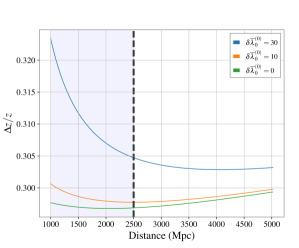
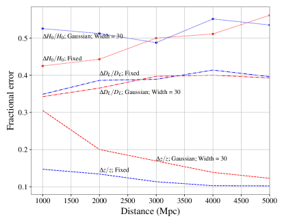
Figure 4: Top Panel: The fractional error in $z$ as a function of the width in $\bar{\lambda}^{(0)}_{0}$ prior obtained using Fisher analysis on the model in Eq. (13). We see that the fractional uncertainty in $z$ follows the trends found in Ref. [10] (analogous to the $\delta\bar{\lambda}^{(0)}_{0}=0$ case). We see that, the fractional error in redshift does not change significantly with change in the width of $\bar{\lambda}^{(0)}_{0}$ prior at large distances from the source. The Fisher approximation is however valid in the high SNR regime, which we assume to be the region of SNR $\gtrsim 30$ shown by the shading. We find similar trends from Bayesian parameter estimation results shown in the bottom panel. Bottom Panel: Fractional statistical uncertainty in the measurement of the redshift, $z$, the luminosity distance, $D_{L}$, and $H_{0}$ when using a Gaussian prior on $\bar{\lambda}^{(0)}_{0}$ versus when using a $\delta$-function prior (fixed) are shown for a few representative parameter-estimation runs in the CE era.

Equation (7) tells us that the effect of statistical measurement uncertainty in $\bar{\lambda}^{(0)}_{0}$ directly affects the measurement of the redshift, $z$. To estimate this effect, we perform a Fisher analysis similar to that of Ref. [10]. For the signal model we use a restricted post-Newtonian(PN) waveform, where we include terms up to 3.5 PN for the point particle contribution [54] and upto 7.5 PN in the tidal contribution in the phase of the waveform [11]. We parametrise our waveform as

$$\tilde{h}(f)=\tilde{h}(f;\mathcal{A},\mathcal{M}_{c},\mathcal{\eta},D_{L},t_{c},\phi_{c},\bar{\lambda}^{(0)}_{0},z),$$ (13)

where $t_{c}$ and $\phi_{c}$ are the coalescence time and phase and $\mathcal{A}$ is the amplitude of the waveform (similar to Ref. [10]). We parameterize the tidal piece of the waveform using the parameterization mentioned in Eq. (1). We use the above signal model and a Gaussian prior on $\bar{\lambda}^{(0)}_{0}$ with few choices of standard deviation to see how the width in the $\bar{\lambda}^{(0)}_{0}$ prior affects the accuracy in the extraction of the redshift $z$. The injected value of $\bar{\lambda}^{(0)}_{0}$ is equal to 200. The result for the fractional uncertainty in redshift is shown in the top panel of Fig. 4. We observe a similar trend in the fractional error in recovery of the redshift as Ref. [10] (the $\delta\bar{\lambda}^{(0)}_{0}=0$ case). When we have a measurement uncertainty, represented by the $\delta\bar{\lambda}^{(0)}_{0}=10,30$ cases, we find that it does not affect the measurement uncertainty of the redshift at larger distances. We note, however, that the Fisher approximation holds true only in the high signal-to-noise limit. In the top panel of Fig. 4 we use a value of SNR $\gtrsim 30$, shown by the shading, as representing the region where the Fisher approximation is valid.

To verify these Fisher estimates, we repeat some of the representative, parameter-estimation runs in the CE era using a Gaussian prior on $\bar{\lambda}^{(0)}_{0}$, around the true value of 200, with a standard deviation of 30. This would correspond to $\sim 15\%$ statistical uncertainty from the value of $\bar{\lambda}^{(0)}_{0}=200$. We show the fractional uncertainty in $H_{0}$, $D_{L}$, $z$ in bottom panel of Fig. 4. In this case we mean $90\%$ intervals by $\Delta z,\Delta D_{L},\Delta H_{0}$. We observe that the redshift error trends from the full parameter-estimation runs are in agreement with the trends of the Fisher estimates. In particular, the fractional error in $H_{0}$ does not change significantly, even when we include a Gaussian prior in $\bar{\lambda}^{(0)}_{0}$. This analysis also agrees with the Fisher uncertainties reported in Messenger and Read. Given these results, we do not expect that a prior statistical uncertainty in the measurement of $\bar{\lambda}^{(0)}_{0}$ will significantly affect the final $H_{0}$ measurement, especially since most detections will be at larger distances in the third-generation detector era.

V.2 Effect of a systematic bias in $\bar{\lambda}^{(0)}_{0}$

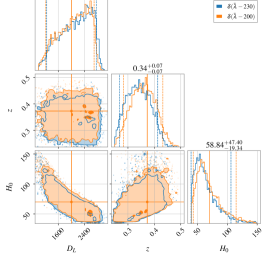
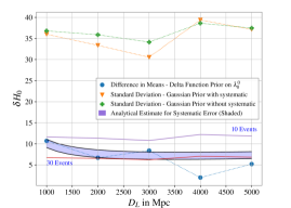
Figure 5: Top panel: Comparison of distance, redshift, and $H_{0}$ measurements for an example parameter estimation run injected at a $D_{L}=2$ Gpc in the CE era. Two cases of recovery are shown – one using a prior at the true value $\delta(\bar{\lambda}^{(0)}_{0}-200)$, and another shifted $\delta(\bar{\lambda}^{(0)}_{0}-230)$ prior. We observe no significant change in the distance recovery, but a systematic shift in the recovery of the redshift; the latter impacts the $H_{0}$ measurement. Bottom panel: The difference in means of the $H_{0}$ measurements between the true and shifted cases by doing a few more parameter estimation runs as above. This is shown by the dotted line with filled circles. We repeat the runs, putting a Gaussian prior with standard deviation of 30 for $\bar{\lambda}^{(0)}_{0}$, centered at the true value of 200, and plot half of the 90% credible interval for $H_{0}$ in dotted line with a plus marker. We repeat one more time with the same width but now centered at 230, and plot half credible region in using dotted lines with inverted triangles. We find that the credible region is not affected by a systematic shift in $\bar{\lambda}^{(0)}_{0}$. Therefore, we consider the former, and show improvements ($\propto 1/\sqrt{N_{\text{det}}}$) as we increase the number of detections, using solid lines. Observe that for $N_{\text{det}}\sim 30$, the statistical improvement hits the boundary of systematic error, shown in blue. We also show the analytical estimate for the systematic error from Eq. (14) using the shading, which roughly agrees with the parameter estimation runs.

Following Eq. (7), a systematic bias in the measurement of $\bar{\lambda}^{(0)}_{0}$ will lead to a biased measurement of $z$, and hence a bias in the inferred value of $H_{0}$. We can estimate this in the following way. Assume first that there is no bias in the measurement of quantities that depend directly on the signal, like masses and tidal deformabilities. If so, any systematic bias in $H_{0}$ will be solely due to an induced bias in $z$ due to the bias in $\bar{\lambda}^{(0)}_{0}$ given the parameterization in Eq. (7). If one considers then a systematic bias shift $\delta\bar{\lambda}^{(0)}_{0}$, one finds from Eq. (7) that

$$\delta\bar{\lambda}=\delta\bar{\lambda}^{(0)}_{0}+\delta\left[\sum_{k=1}^{3}\frac{\bar{\lambda}^{(k)}_{0}}{k!}\left(1-\frac{m_{\text{det}}/m_{0}}{1+z}\right)^{k}\right].$$ (14)

A covariance then arises between $\delta H_{0}$ and $\delta\bar{\lambda}^{(0)}_{0}$ that can be explored by setting $\delta\bar{\lambda}=0=\delta m_{\text{det}}$. The quantity $\delta H_{0}=(\delta H_{0}/\delta\bar{\lambda}^{(0)}_{0})\delta\bar{\lambda}^{(0)}_{0}$ is plotted in Fig. 5 with $\delta\bar{\lambda}^{(0)}_{0}=30$, where the upper (lower) limits of the shading correspond to $m_{\text{source}}=1.3\;(1.5)M_{\odot}$. Observe that the induced error in $H_{0}$ is much smaller than any statistical error reported earlier.

In order to verify this estimate, we repeat some of the representative parameter estimation studies, but this time with models that either have a delta-function or a Gaussian prior that are both peaked at a shifted location of $\bar{\lambda}^{(0)}_{0}=230$. With these priors, the redshift measurement shifts from its true values. An example is shown in the top panel of Fig. 5 where we observe that the recovered redshift is systematically lower for the case when we use the $\delta(\bar{\lambda}^{(0)}_{0}-230)$ prior. The distance measurement is unchanged since its information comes from the amplitude which is not affect due to a biased $\bar{\lambda}^{(0)}_{0}$ measurement. The shift in $z$ shows up as a bias in $H_{0}$. We perform parameter estimation for a few more such injections at different distances with this shifted prior and simply use the difference in means as a benchmark for a systematic error. In the bottom panel of Fig. 5 we denote this shift in the means using the dotted line with filled circle markers. We find that it roughly follows the analytic trend from Eq. (14), shown by the shaded region in the bottom panel of Fig. 5.

In reality, we expect the total uncertainty to be more a combination of statistical and systematic, but as more events are stacked, the statistical error will decrease (as $1/\sqrt{N_{\text{det}}}$ or faster), while the systematic error will not. This then means the latter acts as an uncertainty floor that we must contend with when extracting $H_{0}$. One can then roughly determine how many detections would be needed to reach this floor. In Fig. 5, we consider half of the 90% confidence interval of the $H_{0}$ measurement for our runs here (shown in dotted lines with inverted triangle and plus markers) as the statistical uncertainity, and consider an improvement by $1/\sqrt{N_{\text{det}}}$ for $N_{\text{det}}=10,30$ represented by solid lines in the figure. We see then that the statistical error will become smaller than the systematic after we have stacked $N_{\text{det}}>30$ events. However, it is to be noted that this is only illustrated as an example where there is a systematic bias of 30 from the true value of 200 when measuring $\bar{\lambda}^{(0)}_{0}$.

V.3 Effect of uncertainty in binary-love relations

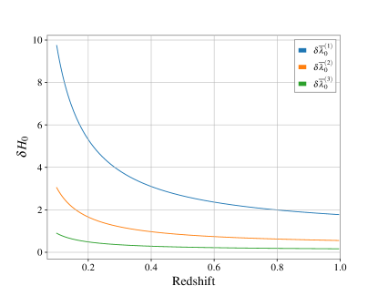
Figure 6: An analytic estimate of the bias in $H_{0}$ caused by assuming the non-universality of the binary-love relations (see Sec. V.3). As an example, here we consider the true EoS to be MPA1 which has the largest residual among the 29 EoSs from the fit in Eq. (3) We see that the error due to loss of universality reduces for $\bar{\lambda}^{(k)}_{0}$ as we increase $k$.

We end this section with an estimate of the systematic error in the inference of $H_{0}$ induced by our assumption that the binary love relations are exact and EoS independent. In order to arrive at a rough estimate, we consider how a bias in $\bar{\lambda}^{(k)}_{0}$, given a value of $\bar{\lambda}^{(0)}_{0}$, would affect our measurements of $H_{0}$. In order to separate this effect from those discussed in the previous subsections, we assume now that $\bar{\lambda}^{(0)}_{0}$ has been measured perfectly. With this in mind, the bias in the $\bar{\lambda}^{(k)}_{0}$ for $k\geq 1$ inside the summation in Eq. (14) leads to a bias in the inferred redshift, and hence a bias in $H_{0}$. This can be estimated by taking a variation of the individual terms as,

$$\delta\left[\frac{\bar{\lambda}^{(k)}_{0}}{k!}\left(1-\frac{m_{\text{det}}/m_{0}}{1+z}\right)^{k}\right]=0.$$ (15)

This expression can be solved for $\delta H_{0}/\delta\bar{\lambda}^{(k)}_{0}$ and multiplied with $\delta\bar{\lambda}^{(k)}_{0}$ to obtain the bias in $H_{0}$. This is shown in Fig. 6. Here, we choose the residuals for the MPA1 EoS as the values for $\delta\bar{\lambda}^{(k)}_{0};\;k\geq 1$. Observe that the systematic error introduced in the extraction of $H_{0}$ is much smaller than the statistical error. From this we conclude that only after more than a certain number of events are stacked ($\sim 30$ in this case), will this systematic error be of any importance. Observe also that the systematic error due to the binary Love relations is smaller for the higher-order terms in the Taylor expansion.

VI Conclusion

This work demonstrates yet another application of universal relations in NSs. Following the proposition by Messenger and Read [10], previous attempts at measuring the distance-redshift relation solely using GWs have relied on the knowledge of the specific NS EoS.  The expansion of the tidal deformability in terms of the source mass is particularly interesting since it breaks the degeneracy between GW frequency and redshift. However, in absence of a priori EoS information, all of the expansion coefficients are free parameters. The $\bar{\lambda}^{(0)}_{0}-\bar{\lambda}^{(k)}_{0}$ relations greatly constrain this degree of freedom. By employing these relations, knowing only a single coefficient determines the rest. This can be particularly useful for setting physically motivated priors on the tidal deformability. In GW astrophysics, previous literature has considered putting flat priors on $\bar{\lambda}_{1,2}$ or $\bar{\Lambda}$. However, another option which is physically motivated prior is an uninformative prior on the free universal expansion coefficient, $\bar{\lambda}^{(0)}_{0}$, which in turn restricts the priors on $\bar{\lambda}_{1,2}$, or $\bar{\Lambda}$. In this work, we employ this technique to GW170817 strain data, and obtain the measurement of $\bar{\lambda}(1.4M_{\odot})$ that is consistent with previous measurements by the LIGO/Virgo collaboration.

The advantage of using the $\bar{\lambda}^{(0)}_{0}-\bar{\lambda}^{(k)}_{0}$ relations is that the tidal deformability is only parameterized by two quantities: $\bar{\lambda}^{(0)}_{0}$ and $m_{\text{source}}$ (or equivalently, $z$). Future multi-messenger observations of GWs from BNSs with simultaneous identification of the redshift would lead to measurements of $\bar{\lambda}^{(0)}_{0}$ that can be combined to give a constrained measurement for this fundamental quantity. Such observations are well motivated based on forecasting studies of different observing scenarios of GW observations [50] combined with development of current and next generation synoptic surveys, and cyber-infrastructure developments.  With a constraint on $\bar{\lambda}^{(0)}_{0}$, the use case can be flipped to now measure the redshift of BNS signals from the tidal deformability measurements. This is advantageous since the method does not rely on any prompt follow-up operations, and is also free from selection effect of host galaxy identification or galaxy catalog incompleteness that has been used in the literature till date.

We demonstrate this technique of measuring the Hubble constant, $H_{0}$, using a synthetic population of detected NS binaries. We also analyze the impact of error in measurement of $H_{0}$ due to the statistical and systematic errors in this prescription. However, aside from GW observations constraining allowed NS EoSs, there are other missions which are also putting stringent measurement of the mass and radii of NSs. Recently, the NICER team reported the discovery of X-ray pulses from massive milli-second pulsars, PSR J0740+6620 and PSR J1614-2230 [58]. The data from PSR J0740+6620 has been used to measure the mass-radius relation of the NS [59, 60, 61]. Such measurements are expected to rule out representative EoSs from the literature that are inconsistent with observables, further reducing the uncertainty in the $\bar{\lambda}^{(0)}_{0}-\bar{\lambda}^{(k)}_{0}$ relations presented here.

Appendix A Implied prior on $\bar{\lambda}_{1,2}$ by $\bar{\lambda}^{(0)}_{0}$

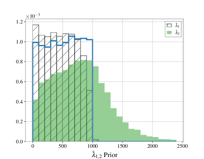
Figure 7: The implied (marginal) priors on the individual tidal deformability parameters due to the uniform prior in $\bar{\lambda}^{(0)}_{0}$ in Sec. III. The prior on $\bar{\lambda}_{1}$ is shown in the hatched histogram, and $\bar{\lambda}_{2}$ is shown in the filled histogram. The $\bar{\lambda}^{(0)}_{0}$ prior is shown in the unfilled histogram.

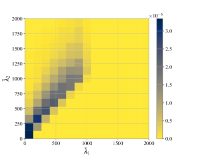
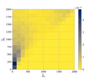
Figure 8: Left panel: Non-marginalized version of Fig. 7. Here, we have used the parameterization using $\bar{\lambda}^{(0)}_{0}-\bar{\lambda}^{(k)}_{0}$ relations from Sec. II. Observe the correlation between $\bar{\lambda}_{1,2}$, which is expected due to the prior information about the masses when imposing a common EoS. Right panel: The prior on implied $\bar{\lambda}_{1,2}$ when using the universal relation between the symmetric and anti-symmetric tidal deformability, $\bar{\lambda}_{s}-\bar{\lambda}_{a}$, relations from YY17. This was used in the EoS-insensitive results reported previously in Ref. [16].

In Sec. III, we did not set an explicit prior on the individual tidal deformabilities, $\bar{\lambda}_{1,2}$ independently. However, the uniform prior on the $\bar{\lambda}^{(0)}_{0}$ parameter along with the prior on the individual component masses imply a prior on the individual tidal deformabilities, $\bar{\lambda}_{1,2}$. We show this in Fig. 7. It should be noted that there are correlations between the two tidal deformabilities based on the priors on the masses. We show this in Fig. 8. On the left panel therein, we see the correlation between the $\bar{\lambda}_{1,2}$. Here, for the mass priors, we use the same mass priors as Sec. III. The correlation is motivated from the fact that in the limit of equal mass components, we expect the tidal deformabilities to be equal. We also note that the prior implied in this work differs from that used in Ref. [16] where instead the symmetric tidal deformability, $\bar{\lambda}_{s}=(\bar{\lambda}_{1}+\bar{\lambda}_{2})/2$ was sampled uniformly, and then $\bar{\lambda}_{a}=(\bar{\lambda}_{1}-\bar{\lambda}_{2})/2$ was obtained using another universal relation, $\bar{\lambda}_{a}=\bar{\lambda}_{a}(\bar{\lambda}_{s},q)$, reported in YY17. We reproduce the implied prior obtained using the latter technique in the right panel of Fig. 8. We attributed the differences in the upper limit value for $\bar{\lambda}^{(0)}_{0}$ between this work and Ref. [16], mentioned in Sec. III due to the difference in priors.

Appendix B Parameter estimation from GW170817 data

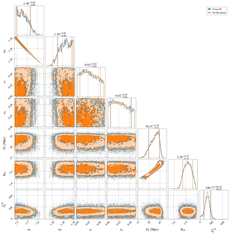
Figure 9: Extended (corner) plot showing pair and marginal parameters from performing Bayesian parameter estimation on GW170817 data discussed in Sec. III. The parameterization of the tidal deformabilities follows Eq. (1). The redshift of the source is fixed to 0.0099. The bottom right posterior for $\bar{\lambda}^{(0)}_{0}$ is the same as Fig. 2 in the main text. We show the distribution of parameters in both cases - when using the fit in Eq. (1) directly, and when including the residual errors from the fit mentioned in the Sec. II.

In Sec. II, we showed the marginalized posterior on the universal quantity, $\bar{\lambda}^{(0)}_{0}$, from performing Bayesian parameter estimation. Here, we show pair-plots and marginalized distributions (corner plot) of some of the other parameters in Fig. 9. The priors on the masses are the marginalized posterior of the detector-frame values reported in GWTC-1. For the luminosity distance, we use a uniform in comoving volume up to 75 Mpc. For the spins, we use the low-spin prior from GWTC-1. The bottom right block is the same as Fig. 2 in the main body of the text. For the BILBY configuration, we use the nested sampling algorithm, DYNESTY, with number of live points nlive = 1500, and number of autocorrelation lengths to reject before accepting a new point, nact = 10. These settings are motivated from settings used in the validation of bilby against GWTC-1 events [63].

Appendix C Trends in $H_{0}$ recovery with inclination

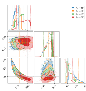
Figure 10: This is an example of $D_{L}$, $z$, and $H_{0}$ measurements for different combinations of the true inclination angle, $\theta_{JN}$, at a fixed distance of 3 Gpc in the Cosmic Explorer era. Note that with increasing true inclination angle, there is increasing support for larger distance values. This is expected since a larger inclination implies a lower injected amplitude, which is recovered as a larger distance. The redshift measurement is not affected since it comes from the phase of the waveform.

In this section we illustrate how the inclination angle affect the distance recovery, which impacts the posterior of $H_{0}$. In Fig. 10, we show the distance, redshift, and $H_{0}$ recovery considering injections at a fixed distance but varying inclination angles. We observe that the recovered distance has support for larger values as the true inclination angle increases. This is expected since edge-on sources have lower SNR compared to face-on sources, and therefore are degenerate with a larger distance recovery. On the other hand, since the redshift is recovered from the phase of the waveform, it is not affected. This implies that the $H_{0}$ recovery is affected in the opposite sense, having support for higher-than-true values for face-on sources and vice versa. However, in all cases, there is support for the true value of $70~{}\text{km s}^{-1}/\text{Mpc}$.

Appendix D Considering alternative redshift priors

Figure 11: Upper panel: The combined measurement of the $H_{0}$, similar to Fig. II for the Cosmic Explorer example. Here, we have reweighted the normalized number count of the recovered events using a redshift prior following uniform in comoving volume (dashed), and that following star formation history (solid). Bottom panel: The contour plot showing the normalized number counts similar to Fig. II for the two alternative priors. We observe that the combined measurement of $H_{0}$ is not significantly affected due to the prior on redshift.

In this appendix, we show the effect of using alternative choices for distances/redshift compared to distributing them uniformly in volume, $\propto D_{L}^{2}$, used in the main body of the text for Fig. II. We consider the Cosmic Explorer example from Sec. IV. We consider two cases – 1) redshift distribution such that the rate is uniform in comoving volume, and 2) it follows the cosmic star formation history [following Eq. 15 from Ref. 64]. We re-weight the luminosity distance of recovered binary systems in Sec. IV using the two priors as shown in Fig. II. For Bayesian parameter estimation, we consider the same representative distance/inclination gridpoints as in the Cosmic Explorer panel of Fig. II, but count them based on the re-weighted heatmap in Fig. II. We find that the combined $H_{0}$ measurement is not affected by the choice of the priors. We also would like to note that while the evolution of the BBH rate has been done [65], the BNS rate has not been constrained strongly due to lack of BNS observations and their relative low distances compared to BBHs. Hence, we feel that our choice made here is justified. The analysis can be redone as further constrains are put on the same.

Appendix E Reweighting the $H_{0}$ posterior

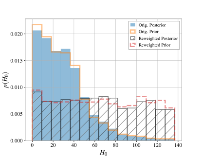
Figure 12: Illustration of obtaining the likelihood from the $H_{0}$ posterior. In this example, we injected a low SNR ($\sim 1$) injection, and perform parameter estimation mentioned in Appendix F. The original prior on $H_{0}$ is shown by solid unfilled histogram, the posterior is shown in filled histogram. The re-weighted prior and posterior are shown as dashed and hatched histograms. The latter is what is expected in absence of any information.

In Sec. IV, we employ the $\bar{\lambda}^{(0)}_{0}-\bar{\lambda}^{(k)}_{0}$ relation, to parameterize the tidal deformability in terms of the redshift $z$. Therefore, one can either sample in $z$, or with the other cosmological parameters fixed in a $\Lambda\text{CDM}$ universe, sample directly in the $H_{0}$. In the former case, putting a prior on $z$ and the luminosity distance, $D_{L}$, implies a prior on $H_{0}$, while in the latter, we directly put a prior on the $H_{0}$. In either case, when combining multiple observations, we need to multiply the likelihoods, dividing out by any imposed or implied prior. In practice putting a uniform prior when sampling (ensuring that the posterior does not rail against the prior boundaries) is equivalent of the likelihood up to a constant factor. We illustrate this using a low signal to noise ratio (SNR $\sim$ 1) event. We put a prior on $D_{L}$ that is uniform in comoving volume up to 5 Gpc, and a uniform prior on redshift $\in[0,0.5]$. The implied prior on $H_{0}$ due to this prior choice is shown in Fig. 12 by the solid, unfilled histogram. Due to the low SNR of the injection in this case, we expect the posterior to be similar to the prior on $H_{0}$. To obtain the likelihood, we need to divide out by the prior, or reweight the samples such that the new prior on $H_{0}$ is flat. In practice this is done by binning the posterior samples and weighting them by the inverse count of the prior distribution. The new re-weighted posterior is shown by the hatched histogram. As expected, this measurement is uninformative i.e., the re-weighted posterior, which in this case is the likelihood, is flat.

Appendix F PARALLEL_BILBY configuration for BNS simulations

For Sec. IV, we make use of the PARALLEL_BILBY framework [53] which is an extension of BILBY to scale out the analysis using Message Passing Interface (MPI)  to an entire high-performance cluster. We use a fiducial binary with a source-frame chirp mass of $\mathcal{M}_{c}=1.17~{}M_{\odot}$ and mass-ratio, $q=0.9$ for all of our synthetic injections. The signal duration is 128s. While BNS signals will last much longer during the CE era, the 5PN tidal terms only become pronounced close to merger. The injected redshifted chirp mass is obtained as, $(1+z^{\text{inj}})\mathcal{M}_{c}^{\text{inj}}$, where $z^{\text{inj}}$ is determined from the injected luminosity distance that assumed true flat-$\Lambda\text{CDM}(H_{0}=70~{}\text{km s}^{-1}/\text{Mpc},\Omega_{m0}=0.3)$ cosmology. For sampling, we use a prior that is uniform in detector-frame chirp mass between $(1+z^{\text{inj}})\mathcal{M}_{c}^{\text{inj}}\pm 0.1~{}M_{\odot}$, and a prior uniform in mass-ratio $\in[0.65,1]$. We ignore spins (set them to zero), and use delta function priors at zero on spin when sampling. We also fix the sky-location of the source. The prior for distance is uniform in comoving volume up to twice the injected distance. We use a stationary Gaussian noise realization for each of our detector era. For the O5 and CE results in Fig. II, we impose a uniform prior on the redshift, and get the individual likelihoods using the technique mentioned in Appendix E. For the Voyager results, we sample directly in $H_{0}$ using a uniform prior $\in[1,300]~{}\text{km s}^{-1}/\text{Mpc}$.

References

- Schutz [1986] B. F. Schutz, Nature 323, 310 (1986).
- Holz and Hughes [2005] D. E. Holz and S. A. Hughes, ApJ 629, 15 (2005), eprint astro-ph/0504616.
- Gray et al. [2020] R. Gray, I. M. Hernandez, H. Qi, A. Sur, P. R. Brady, H.-Y. Chen, W. M. Farr, M. Fishbach, J. R. Gair, A. Ghosh, et al., Phys. Rev. D 101, 122001 (2020), eprint 1908.06050.
- Aasi et al. [2015] J. Aasi, B. P. Abbott, R. Abbott, T. Abbott, M. R. Abernathy, K. Ackley, C. Adams, T. Adams, P. Addesso, and et al., Classical and Quantum Gravity 32, 074001 (2015), ISSN 1361-6382, URL http://dx.doi.org/10.1088/0264-9381/32/7/074001.
- Acernese et al. [2014] F. Acernese, M. Agathos, K. Agatsuma, D. Aisa, N. Allemandou, A. Allocca, J. Amarni, P. Astone, G. Balestri, G. Ballardin, et al., Classical and Quantum Gravity 32, 024001 (2014), ISSN 1361-6382, URL http://dx.doi.org/10.1088/0264-9381/32/2/024001.
- Abbott et al. [2017a] B. P. Abbott, R. Abbott, T. D. Abbott, F. Acernese, K. Ackley, C. Adams, T. Adams, P. Addesso, R. X. Adhikari, V. B. Adya, et al., Phys. Rev. Lett. 119, 161101 (2017a), eprint 1710.05832.
- Abbott et al. [2017b] B. P. Abbott, R. Abbott, T. D. Abbott, F. Acernese, K. Ackley, C. Adams, T. Adams, P. Addesso, R. X. Adhikari, V. B. Adya, et al., Nature 551, 85 (2017b), eprint 1710.05835.
- Fishbach et al. [2019] M. Fishbach, R. Gray, I. Magaña Hernandez, H. Qi, A. Sur, F. Acernese, L. Aiello, A. Allocca, M. A. Aloy, A. Amato, et al., ApJ 871, L13 (2019), eprint 1807.05667.
- Verde et al. [2019] L. Verde, T. Treu, and A. G. Riess, Nature Astronomy 3, 891 (2019), eprint 1907.10625.
- Messenger and Read [2012] C. Messenger and J. Read, Phys. Rev. Lett. 108, 091101 (2012), eprint 1107.5725.
- Damour et al. [2012] T. Damour, A. Nagar, and L. Villain, Phys. Rev. D 85, 123007 (2012), eprint 1203.4352.
- Del Pozzo et al. [2013] W. Del Pozzo, T. G. F. Li, M. Agathos, C. Van Den Broeck, and S. Vitale, Phys. Rev. Lett. 111, 071101 (2013), eprint 1307.8338.
- Agathos et al. [2015] M. Agathos, J. Meidam, W. Del Pozzo, T. G. F. Li, M. Tompitak, J. Veitch, S. Vitale, and C. Van Den Broeck, Phys. Rev. D 92, 023012 (2015), eprint 1503.05405.
- Yagi and Yunes [2016] K. Yagi and N. Yunes, Classical and Quantum Gravity 33, 13LT01 (2016), eprint 1512.02639.
- Yagi and Yunes [2017] K. Yagi and N. Yunes, Classical and Quantum Gravity 34, 015006 (2017), eprint 1608.06187.
- Abbott et al. [2018] B. P. Abbott, R. Abbott, T. D. Abbott, F. Acernese, K. Ackley, C. Adams, T. Adams, P. Addesso, R. X. Adhikari, V. B. Adya, et al., Phys. Rev. Lett. 121, 161101 (2018), eprint 1805.11581.
- Miller et al. [2019] M. C. Miller, F. K. Lamb, A. J. Dittmann, S. Bogdanov, Z. Arzoumanian, K. C. Gendreau, S. Guillot, A. K. Harding, W. C. G. Ho, J. M. Lattimer, et al., ApJ 887, L24 (2019), eprint 1912.05705.
- Fishbach et al. [2019] M. Fishbach, R. Gray, I. M. Hernandez, H. Qi, A. Sur, F. Acernese, L. Aiello, A. Allocca, M. A. Aloy, A. Amato, et al., The Astrophysical Journal 871, L13 (2019), ISSN 2041-8213, URL http://dx.doi.org/10.3847/2041-8213/aaf96e.
- Soares-Santos et al. [2019] M. Soares-Santos, A. Palmese, W. Hartley, J. Annis, J. Garcia-Bellido, O. Lahav, Z. Doctor, M. Fishbach, D. E. Holz, H. Lin, et al., The Astrophysical Journal 876, L7 (2019), ISSN 2041-8213, URL http://dx.doi.org/10.3847/2041-8213/ab14f1.
- Abbott et al. [2020a] R. Abbott, T. Abbott, S. Abraham, F. Acernese, K. Ackley, C. Adams, R. Adhikari, V. Adya, C. Affeldt, M. Agathos, et al., Physical Review Letters 125 (2020a), ISSN 1079-7114, URL http://dx.doi.org/10.1103/PhysRevLett.125.101102.
- Graham et al. [2020] M. Graham, K. Ford, B. McKernan, N. Ross, D. Stern, K. Burdge, M. Coughlin, S. Djorgovski, A. Drake, D. Duev, et al., Physical Review Letters 124 (2020), ISSN 1079-7114, URL http://dx.doi.org/10.1103/PhysRevLett.124.251102.
- Mukherjee et al. [2020] S. Mukherjee, A. Ghosh, M. J. Graham, C. Karathanasis, M. M. Kasliwal, I. M. Hernandez, S. M. Nissanke, A. Silvestri, and B. D. Wandelt, First measurement of the hubble parameter from bright binary black hole gw190521 (2020), eprint 2009.14199.
- Chen et al. [2020] H.-Y. Chen, C.-J. Haster, S. Vitale, W. M. Farr, and M. Isi, arXiv e-prints arXiv:2009.14057 (2020), eprint 2009.14057.
- Carroll [2019] S. M. Carroll, Spacetime and Geometry (Cambridge University Press, 2019), ISBN 978-0-8053-8732-2, 978-1-108-48839-6, 978-1-108-77555-7.
- Blanchet et al. [1995] L. Blanchet, T. Damour, B. R. Iyer, C. M. Will, and A. G. Wiseman, Physical Review Letters 74, 3515–3518 (1995), ISSN 1079-7114, URL http://dx.doi.org/10.1103/PhysRevLett.74.3515.
- Flanagan and Hinderer [2008] É. É. Flanagan and T. Hinderer, Phys. Rev. D 77, 021502 (2008), eprint 0709.1915.
- Hinderer [2008] T. Hinderer, The Astrophysical Journal 677, 1216 (2008), URL https://doi.org/10.1086/533487.
- De et al. [2018] S. De, D. Finstad, J. M. Lattimer, D. A. Brown, E. Berger, and C. M. Biwer, Phys. Rev. Lett. 121, 091102 (2018), [Erratum: Phys. Rev. Lett.121,no.25,259902(2018)], eprint 1804.08583.
- Yagi and Yunes [2013a] K. Yagi and N. Yunes, Science 341, 365–368 (2013a), ISSN 1095-9203, URL http://dx.doi.org/10.1126/science.1236462.
- Yagi and Yunes [2013b] K. Yagi and N. Yunes, Physical Review D 88 (2013b), ISSN 1550-2368, URL http://dx.doi.org/10.1103/PhysRevD.88.023009.
- Yagi and Yunes [2017] K. Yagi and N. Yunes, Phys. Rept. 681, 1 (2017), eprint 1608.02582.
- Doneva and Pappas [2018] D. D. Doneva and G. Pappas, Astrophys. Space Sci. Libr. 457, 737 (2018), eprint 1709.08046.
- Demorest et al. [2010] P. B. Demorest, T. Pennucci, S. M. Ransom, M. S. E. Roberts, and J. W. T. Hessels, Nature 467, 1081 (2010), eprint 1010.5788.
- Antoniadis et al. [2013] J. Antoniadis, P. C. Freire, N. Wex, T. M. Tauris, R. S. Lynch, et al., Science 340, 6131 (2013), eprint 1304.6875.
- Cromartie et al. [2019] H. T. Cromartie et al. (NANOGrav), Nature Astron. 4, 72 (2019), eprint 1904.06759.
- Read et al. [2009] J. S. Read, B. D. Lackey, B. J. Owen, and J. L. Friedman, Physical Review D 79 (2009), ISSN 1550-2368, URL http://dx.doi.org/10.1103/PhysRevD.79.124032.
- Jaranowski and Krolak [1994] P. Jaranowski and A. Krolak, Phys. Rev. D 49, 1723 (1994), URL https://link.aps.org/doi/10.1103/PhysRevD.49.1723.
- Cutler and Flanagan [1994] C. Cutler and É. E. Flanagan, Physical Review D 49, 2658–2697 (1994), ISSN 0556-2821, URL http://dx.doi.org/10.1103/PhysRevD.49.2658.
- van der Sluys et al. [2008] M. V. van der Sluys, C. Röver, A. Stroeer, V. Raymond, I. Mandel, N. Christensen, V. Kalogera, R. Meyer, and A. Vecchio, The Astrophysical Journal 688, L61 (2008), URL https://doi.org/10.1086/595279.
- Veitch et al. [2012] J. Veitch, I. Mandel, B. Aylott, B. Farr, V. Raymond, C. Rodriguez, M. van der Sluys, V. Kalogera, and A. Vecchio, Physical Review D 85 (2012), ISSN 1550-2368, URL http://dx.doi.org/10.1103/PhysRevD.85.104045.
- Veitch et al. [2015] J. Veitch, V. Raymond, B. Farr, W. Farr, P. Graff, S. Vitale, B. Aylott, K. Blackburn, N. Christensen, M. Coughlin, et al., Physical Review D 91 (2015), ISSN 1550-2368, URL http://dx.doi.org/10.1103/PhysRevD.91.042003.
- Dietrich et al. [2019] T. Dietrich, S. Khan, R. Dudi, S. J. Kapadia, P. Kumar, A. Nagar, F. Ohme, F. Pannarale, A. Samajdar, S. Bernuzzi, et al., Phys. Rev. D 99, 024029 (2019), URL https://link.aps.org/doi/10.1103/PhysRevD.99.024029.
- Abbott et al. [2019] B. P. Abbott, R. Abbott, T. D. Abbott, F. Acernese, K. Ackley, C. Adams, T. Adams, P. Addesso, R. X. Adhikari, V. B. Adya, et al., Physical Review X 9, 011001 (2019), eprint 1805.11579.
- Abbott et al. [2019] B. Abbott, R. Abbott, T. Abbott, S. Abraham, F. Acernese, K. Ackley, C. Adams, R. Adhikari, V. Adya, C. Affeldt, et al., Physical Review X 9 (2019), ISSN 2160-3308, URL http://dx.doi.org/10.1103/PhysRevX.9.031040.
- Levan et al. [2017] A. J. Levan, J. D. Lyman, N. R. Tanvir, J. Hjorth, I. Mandel, E. R. Stanway, D. Steeghs, A. S. Fruchter, E. Troja, S. L. Schrøder, et al., The Astrophysical Journal 848, L28 (2017), URL https://doi.org/10.3847/2041-8213/aa905f.
- Ashton et al. [2019] G. Ashton, M. Hübner, P. D. Lasky, C. Talbot, K. Ackley, S. Biscoveanu, Q. Chu, A. Divakarla, P. J. Easter, B. Goncharov, et al., ApJS 241, 27 (2019), eprint 1811.02042.
- Speagle [2020] J. S. Speagle, MNRAS 493, 3132 (2020), eprint 1904.02180.
- Ivezić et al. [2019] v. Ivezić, S. M. Kahn, J. A. Tyson, B. Abel, E. Acosta, R. Allsman, D. Alonso, Y. AlSayyad, S. F. Anderson, J. Andrew, et al., The Astrophysical Journal 873, 111 (2019), ISSN 1538-4357, URL http://dx.doi.org/10.3847/1538-4357/ab042c.
- Chen et al. [2018] H.-Y. Chen, M. Fishbach, and D. E. Holz, Nature 562, 545–547 (2018), ISSN 1476-4687, URL http://dx.doi.org/10.1038/s41586-018-0606-0.
- Abbott et al. [2020b] B. P. Abbott, R. Abbott, T. D. Abbott, S. Abraham, F. Acernese, K. Ackley, C. Adams, V. B. Adya, C. Affeldt, and et al., Living Reviews in Relativity 23 (2020b), ISSN 1433-8351, URL http://dx.doi.org/10.1007/s41114-020-00026-9.
- Abbott et al. [2017] B. P. Abbott, R. Abbott, T. D. Abbott, M. R. Abernathy, K. Ackley, C. Adams, P. Addesso, R. X. Adhikari, V. B. Adya, C. Affeldt, et al., Classical and Quantum Gravity 34, 044001 (2017), ISSN 1361-6382, URL http://dx.doi.org/10.1088/1361-6382/aa51f4.
- Schutz [2011] B. F. Schutz, Classical and Quantum Gravity 28, 125023 (2011), ISSN 1361-6382, URL http://dx.doi.org/10.1088/0264-9381/28/12/125023.
- Smith et al. [2020] R. J. E. Smith, G. Ashton, A. Vajpeyi, and C. Talbot, Monthly Notices of the Royal Astronomical Society 498, 4492–4502 (2020), ISSN 1365-2966, URL http://dx.doi.org/10.1093/mnras/staa2483.
- Arun et al. [2005] K. G. Arun, B. R. Iyer, B. S. Sathyaprakash, and P. A. Sundararajan, Phys. Rev. D 71, 084008 (2005), URL https://link.aps.org/doi/10.1103/PhysRevD.71.084008.
- Taylor and Gair [2012] S. R. Taylor and J. R. Gair, Physical Review D 86 (2012), ISSN 1550-2368, URL http://dx.doi.org/10.1103/PhysRevD.86.023502.
- Mukherjee et al. [2021] S. Mukherjee, B. D. Wandelt, S. M. Nissanke, and A. Silvestri, Physical Review D 103 (2021), ISSN 2470-0029, URL http://dx.doi.org/10.1103/PhysRevD.103.043520.
- Mastrogiovanni et al. [2021] S. Mastrogiovanni, K. Leyde, C. Karathanasis, E. Chassande-Mottin, D. A. Steer, J. Gair, A. Ghosh, R. Gray, S. Mukherjee, and S. Rinaldi, Cosmology in the dark: On the importance of source population models for gravitational-wave cosmology (2021), eprint 2103.14663.
- Wolff et al. [2021] M. T. Wolff, S. Guillot, S. Bogdanov, P. S. Ray, M. Kerr, Z. Arzoumanian, K. C. Gendreau, M. C. Miller, A. J. Dittmann, W. C. G. Ho, et al., arXiv e-prints arXiv:2105.06978 (2021), eprint 2105.06978.
- Miller et al. [2021] M. C. Miller, F. K. Lamb, A. J. Dittmann, S. Bogdanov, Z. Arzoumanian, K. C. Gendreau, S. Guillot, W. C. G. Ho, J. M. Lattimer, M. Loewenstein, et al., arXiv e-prints arXiv:2105.06979 (2021), eprint 2105.06979.
- Riley et al. [2021] T. E. Riley, A. L. Watts, P. S. Ray, S. Bogdanov, S. Guillot, S. M. Morsink, A. V. Bilous, Z. Arzoumanian, D. Choudhury, J. S. Deneva, et al., arXiv e-prints arXiv:2105.06980 (2021), eprint 2105.06980.
- Raaijmakers et al. [2021] G. Raaijmakers, S. K. Greif, K. Hebeler, T. Hinderer, S. Nissanke, A. Schwenk, T. E. Riley, A. L. Watts, J. M. Lattimer, and W. C. G. Ho, arXiv e-prints arXiv:2105.06981 (2021), eprint 2105.06981.
- Abbott et al. [2021a] R. Abbott, T. D. Abbott, S. Abraham, F. Acernese, K. Ackley, C. Adams, R. X. Adhikari, V. B. Adya, C. Affeldt, M. Agathos, et al., SoftwareX 13, 100658 (2021a), ISSN 2352-7110, URL http://dx.doi.org/10.1016/j.softx.2021.100658.
- Romero-Shaw et al. [2020] I. M. Romero-Shaw, C. Talbot, S. Biscoveanu, V. D’Emilio, G. Ashton, C. P. L. Berry, S. Coughlin, S. Galaudage, C. Hoy, M. Hübner, et al., Monthly Notices of the Royal Astronomical Society 499, 3295–3319 (2020), ISSN 1365-2966, URL http://dx.doi.org/10.1093/mnras/staa2850.
- Madau and Dickinson [2014] P. Madau and M. Dickinson, Annual Review of Astronomy and Astrophysics 52, 415–486 (2014), ISSN 1545-4282, URL http://dx.doi.org/10.1146/annurev-astro-081811-125615.
- Abbott et al. [2021b] R. Abbott, T. D. Abbott, S. Abraham, F. Acernese, K. Ackley, A. Adams, C. Adams, R. X. Adhikari, V. B. Adya, C. Affeldt, et al., The Astrophysical Journal Letters 913, L7 (2021b), ISSN 2041-8213, URL http://dx.doi.org/10.3847/2041-8213/abe949.