A note on the interpretation of the statistical analysis of the scaling relation
Abstract
In the context of scaling relations between Supermassive Black Holes and host-galaxy properties, we aim to enhance the comparison between and relations from a statistical point of view. First, it is suggested to take into account the predictive accuracy of the scaling relation, in addition to the classical measures of goodness of fit. Here, prediction accuracy is fairly evaluated according to a leave-one-out cross-validation strategy. Then, we spread more light on the analysis of residuals from the fitted scaling relation, in order to provide more useful information on the role played by the different variables in their correlation with the black hole mass. The findings from six samples are discussed.
Corresponding author: A. L. Iannella - antonellalucia.iannella@unisannio.it
Keywords Host Galaxies; SMBH; Masses of Galaxies; Prediction; Residuals
1 Introduction
It is well ascertained that at the center of local galaxies there is a supermassive black hole (SMBH, ) (Ferrarese and Ford, 2005; Kormendy and Richstone, 1995; Richstone et al., 1998). The SMBH growth and the bulge formation regulate each other (Ho, 2004). The association between the mass of a SMBH with the properties of the hosting galaxy has been extensively studied in the literature. In particular, the interest focused on the study of the correlation with characteristics such as the bulge luminosity or mass, the velocity dispersion, the effective radius, the Sérsic index, the kinetic energy, etc. (Aller and Richstone, 2007; Berrier et al., 2013; Burkert and Tremaine, 2010; Feoli and Mele, 2005, 2007; Ferrarese and Merritt, 2000; Gebhardt et al., 2000, 2003; Graham et al., 2001; Graham and Driver, 2005, 2007; Gültekin et al., 2009; Häring and Rix, 2004; Kormendy and Richstone, 1995; Laor, 2001; Lauer et al., 2007; Magorrian et al., 1998; Marconi et al., 2001; Marconi and Hunt, 2003; Merritt and Ferrarese, 2001; Richstone et al., 1998; Seigar et al., 2008; Snyder et al., 2011; Soker and Meiron, 2011; Tremaine et al., 2002; van der Marel, 1999; Wandel, 2002). Among all the proposed relations, we studied carefully the performances of the correlation with kinetic energy, as first found by Feoli and Mele in 2005 (Feoli and Mele, 2005). The reason is that this relation exhibits solid theoretical foundations and can play the role of an HR diagram for galaxies (Feoli and Mancini, 2009; Mancini and Feoli, 2012). Furthermore, it has already shown to predict the masses of SMBH better than other relations in some particular cases (Benedetto et al., 2013). In this paper, the objective is to analyze the predictive power of the scaling relation between the mass of a SMBH and kinetic energy and to enhance the statistical analyses in Iannella and Feoli (2020). Then, we will follow two main paths of investigation:
-
1.
we consider the predictive reliability of the scaling relations and , that is fairly measured by leave-one-out cross-validation, as described in Sect. 3, in addition to the classical goodness of fit measures;
-
2.
we discuss more in depth the analysis of residuals from the fitted scaling relations. In particular, in Sect. 4 we give an appropriate understanding of the comparison among correlations developed in Barausse et al. (2017), Bernardi et al. (2007), Hopkins et al. (2007a, b) and Shankar et al. (2016, 2019), aimed to measure the relative importance of the variables that may be included in the scaling relation.
The analysis refers to six samples, that are listed in Sect. 2: five samples have been already considered in Iannella and Feoli (2020) and one comes from Kormendy and Ho (2013). The results about goodness of fit and prediction accuracy of the scaling relations are presented and discussed in Sect. 5. The residual analyses for each sample are considered in Sect. 6, that provide important information on the role played by the different variables in the correlations under investigation. Some concluding remarks follow in Sect. 7.
2 Samples
The analyses concern the five samples from Iannella and Feoli (2020) and one more sample collected in Kormendy and Ho (2013). The results regarding the first five samples are expected to improve over the findings from Feoli and Mele (2005) and Iannella and Feoli (2020). In contrasts, the last sample has not been studied yet, because we planned to include it in an upcoming work related to the role of pseudobulges. Moreover, it is not our intention to modify or comment the results by Kormendy and Ho (2013) (see also Saglia et al. (2016)), but we only aim to offer more insights on some aspects of the statistical analysis. All the six samples have been made available at http://people.ding.unisannio.it/feoli/IF2020.zip.
Here, a brief description of the main characteristics of the six samples follows:
-
the 1st Sample is obtained by taking into consideration the data shared by two datasets: one from Cappellari et al. (2013), that is a sample of early-type galaxies, from which we take the mass of each galaxy with the respective velocity dispersion, and the other from van den Bosch (2016), from which we take the relative mass of the supermassive black hole. The sample is thus made up of 47 galaxies, excluding NGC4429, as its morphological classification is doubtful, and, as regards the NGC4486, we preferred to insert the most recent data obtained for the mass of its SMBH (The Event Horizon Telescope Collaboration, 2019).
-
The 2nd Sample is made up of 174 galaxies, obtained starting from the van den Bosch’s sample (van den Bosch, 2016), but excluding those galaxies whose mass of the SMBH shows a relative error on greater than or equal to 1 (Beltramonte et al., 2019), NGC404, since its mass is too low for an SMBH and NGC4486b which “deviates strongly from any correlation involving the mass of its black hole” Saglia et al. (2016). Finally, we also preferred to exclude NGC221, NGC1277, NGC1316, NGC5845 and UGC1841.
-
The 3rd Sample consists only of the 108 early-type galaxies in the 2nd Sample.
-
The 5th Sample consists of all the data as given in Saglia et al. (2016), choosing the same galaxies as in the previous sample.
-
The 6th Sample is obtained considering the sample discussed in Kormendy and Ho (2013), but reduced to galaxies after excluding the pseudobulges.
Both van den Bosch’s samples do not explicitly contain the masses of the galaxies but include the effective radius of the host spheroidal component and the velocity dispersion of the host galaxy. Then, the mass is computed as
| (1) |
where is the gravitational constant (Cappellari et al., 2006).
3 Model fitting and prediction
The scaling relations we aim to fit to the data at hand are of the type
| (2) |
where is the response, the explanatory variable (or covariate), is the error term. According to an ordinary least squares (OLS) framework, it is assumed that the error term has null expected value and a constant variance that we denote by . It is common to refer to as the intrinsic scatter.
The slope parameter is a direct measure of the strength of the linear association between the response and the covariate . The OLS estimate of the slope parameter is given by
| (3) |
where is the covariance among and , and are the standard deviation of and , respectively, obtained as the square root of the corresponding variances and . It can be noted that the estimate of the slope parameter can be expressed in terms of the sample Pearson linear correlation coefficient . Let
| (4) |
be the fitted model. Then, the fitted values are , . In expression (4) above, we use the symbol rather than to stress that, according to the hypothesis underlying model (2), we are fitting the conditional expected value of the response variable given the value of the explanatory variable.
The goodness of fit is commonly assessed through the coefficient of determination . It measures the share of total variability, as measured by the total sum of squares (also called deviance) , where is the sample mean, of the response variable explained by the fitted regression model. Actually, the total sum of squares can be decomposed as
Then,
| (5) |
where denotes the sum of squared errors
| (6) |
and is the classical estimate of the intrinsic scatter. We find that . In order to assess the validity of the fitted model, it is recommended to test the null hypothesis according to the statistic , where is the standard error and is distributed according to a Student’s distribution. The model is valid when there is evidence supporting the importance of the covariate to explain part of the variability of the response, as measured by a small enough p-value .
In addition to measure the quality of the fitted scaling relation in terms of goodness of fit, in this paper we also suggest to evaluate the prediction accuracy of the fitted model when the task is that of predicting new response values. Here, the prediction ability is fairly measured by cross-validation. The basic idea behind cross-validation is to split the data into two subsets: one is used as a training sample, i.e. to build the model, the other acts as a test sample (or validation sample), to assess and validate the model. This validation is performed by comparing the test data with their predictions stemming from the model fitted on the train data. The splitting of the data is supposed to be executed randomly and repeated several times to get a fair estimate of the prediction accuracy of the fitted model. Actually, cross-validation is a resampling method.
In this paper we used leave-one-out cross-validation. The model is fitted times, every time omitting one observation. Then, for every fitted model, a prediction of the previously discarded observation is obtained as , where the subscript is used to stress the fact that estimation is based on the sample without the ith observation. Prediction accuracy is measured by the prediction mean squared error
| (7) |
4 Residuals Analysis and model comparison
According to Barausse et al. (2017), Bernardi et al. (2007), Hopkins et al. (2007a, b) and Shankar et al. (2016, 2019), one way to establish the relative importance of one covariate with respect to another covariate in the linear relationship with the variable , and check if the inclusion of the extra explanatory variable in the linear model (2) is able to improve the fitted model, is to compare correlations among residuals. Correlations among residuals from scaling relations will be called conditional correlations. The technique works as follows:
-
1.
fit the regression of over and get residuals
(8) -
2.
fit the regression of on according to the model and get residuals
(9) -
3.
consider the linear correlation between the residuals from the two fitted models, and respectively, that we denote ;
-
4.
repeat the procedure by exchanging the role of and and get ;
-
5.
compare conditional correlation coefficients: if
then is more importantly correlated with relatively to .
In order to give more insights on this type of residual analysis, it is worth to remark some statistical aspects that have been somewhat neglected in the papers cited above and may affect the discussion about the results. Actually, a fair comparison between the conditional correlation coefficients should take into account the uncertainty that characterizes the estimates of conditional correlations driven by the fitted models. In other words, the comparison can not rely only on point estimates of conditional correlations, but on suitable statistical tests and, in a completely equivalent fashion, reporting confidence intervals. Here, confidence intervals are obtained according to the classical Fisher Z test for linear correlation.
The comparison between conditional correlations does not only lead to state that one variable can be more important and fundamental in the scaling relation with respect to the other, but also to verify if the assumed model can be improved significantly in terms of goodness of fit by the inclusion of the extra variable. Assume that we fit the scaling relation in (2). Actually, when zero is outside the confidence interval around , this means that the inclusion of leads to a significant reduction in the residual sum of squared errors (at the level ) and, hence, to an improvement of the model in terms of goodness of fit as measured by and, likely, in predictive accuracy.
Let us assume that is also important. Omitting implies a bias in the estimate of the slope parameter that is equal to the fitted slope of the regression of on , that is . Then, the larger the correlation, the larger the omitted variable bias. Table 1 gives the linear correlation coefficient between kinetic energy and velocity dispersion (both on a log scale) for each Sample under study. A strong correlation emerges between and .
Since, for van den Bosch sample, the kinetic energy is
| (10) |
then a strong correlation between the effective radius of host spheroidal component Re and the velocity dispersion exists. If this relation is linear, the slopes of the and relations should differ by a factor of 5. However, this is not always tha case. Actually, we verified with the second sample containing 174 galaxies, that the fitted slope of the relation is , that differs significantly from the slope equal to found in the work of Bernardi et al. (2003).
| Sample | |||
|---|---|---|---|
| Cappellari | 0.912 | ||
| van den Bosch_174 | 0.939 | ||
| van den Bosch_108 | 0.945 | ||
| de Nicola-Saglia | 0.937 | ||
| Saglia | 0.937 | ||
| Kormendy-Ho | 0.948 |
The conditional correlation is proportional to the estimate of the slope of the regression of the residuals from step 1 over the residuals from step 2 above. Let denote this estimate as . It can be proved that where is the coefficient of the model
| (11) |
and the corresponding least squares estimate. This result follows from the Frisch-Waugh theorem (Stock and Watson, 2015). The reader is also pointed to Shankar et al. (2016) and the interesting Appendix B in Shankar et al. (2017).
The inclusion of an extra covariate always lead to an improvement in terms of goodness of fit, in the sense that increases and the residual sum of squared errors becomes smaller. However, one is expected to check if this reduction is large enough to assess the importance of . According to the residual analysis described so far, the reduction is significant when the confidence interval around does not include zero. In an equivalent fashion, one could fit the complete model in (11) and check the significance of the test of nullity about the slope coefficient . To this end, one should use a classical Students’ t test with degrees of freedom, denoted by .
In a completely equivalent fashion, the relative importance of one explanatory variable with respect to the other can be directly assessed by measuring the reduction in the residual sum of squared errors. In other words, we are interested in the difference
| (12) |
where is the sum of squared errors from the fitted model with only or and is the sum of squares from model (11). In order to verify if the reduction is large enough to assess the importance of the extra explanatory variable, we consider the test statistic
| (13) |
where . The p-value
| (14) |
is a direct measure of evidence, where is a Fisher random variable with one and degrees of freedom. The test is significant when the p-value is small enough. The equivalence between this approach and the strategy based on test the hypothesis (or ) in model (11) can be remarked by noting that .
To sum up, comparing the relative importance of the variable with respect to the variable results in fitting the complete model (11). The comparison can be pursued in an equivalent fashion according to inferences (tests or confidence intervals) on:
-
1.
the coefficients in the complete model;
-
2.
the reduction in the residual sum of squared errors;
-
3.
conditional correlations.
5 Fitted scaling relations: empirical results
In this section we present and discuss the results we obtained for each sample introduced in Sect. 2 for what concerns goodness of fit and prediction accuracy of the scaling relations and . To be precise, both the response and the covariate are on a logarithmic scale. The results are based on R routines and codes, whereas in Iannella and Feoli (2020) the OLS fit was obtained from Mathematica and other fits were obtained from the LINMIX_ERR (Kelly, 2007) and MPFITEXY (Tremaine et al., 2002) routines. The latter techniques have not been considered here, but prediction accuracy could have been evaluated by leave-one-out cross-validation as well.
As a general comment, the scaling relation performs quite satisfactory when compared to the classical one. The entries in Table 2 allow the comparison among the considered scaling relations, both in terms of goodness of fit and prediction error. The former can be assessed looking at the value of or, in an equivalent fashion, and the corresponding . The latter through the value and the corresponding . A general advise is to prefer the model returning the smallest fitted intrinsic scatter (that means larger ) and prediction error. In this respect, there could be evidence supporting the validity of both fitted models but one can still provide (even slight) superior goodness of fit and prediction accuracy. As one referees pointed out, it worth noting that the sum of squared (prediction) errors are not comparable across samples, whereas this is true for the fitted intrinsic scatter or the prediction error.
| Scaling relation | |||||||
|---|---|---|---|---|---|---|---|
| 1st Sample: Cappellari | |||||||
| 3.88 | 0.96 | 0.413 | |||||
| -2.75 | 4.88 | 0.714 | 8.56 | ||||
| 2nd Sample: van den Bosch_174 | |||||||
| 3.52 | 0.95 | 0.569 | |||||
| -2.91 | 4.89 | 0.702 | 48.77 | ||||
| 3rd Sample: van den Bosch_108 | |||||||
| 4.17 | 0.86 | 0.423 | |||||
| -2.44 | 4.73 | 0.766 | 19.12 | ||||
| 4th sample: De Nicola - Saglia | |||||||
| 5.19 | 0.72 | 0.387 | |||||
| -2.94 | 4.92 | 0.830 | 12.11 | ||||
| 5th Sample: Saglia | |||||||
| 5.17 | 0.72 | 0.392 | |||||
| -3.05 | 4.97 | 0.832 | 12.26 | ||||
| 6th Sample: Kormendy - Ho | |||||||
| 4.97 | 0.78 | 0.274 | |||||
| -1.39 | 4.29 | 0.837 | 5.16 | ||||
In details, these are the results for each of the six considered samples.
-
Cappellari. The entries in Table 2 state that the relation exhibits a quite comparable behavior with the both in terms of intrinsic error (goodness of fit) and prediction error. The difference in terms of fitted intrinsic scatter (and ) is negligible whereas the former scaling relation exhibits a lower prediction error than the latter.
-
van den Bosch_174. In this sample, the situation is different from the previous one. The relation outperforms the relation both in terms of goodness of fit and prediction error with a rate of explained variability, whereas it is for the latter.
-
van den Bosch_108. From Table 2, the relation shows slightly better performances in terms of goodness of fit and prediction accuracy.
-
de Nicola - Saglia. The relation performs better than the scaling relation both in terms of goodness of fit and prediction error: explained variability of the former is about compared to and the difference in the sum of squared prediction errors is not negligible.
-
Saglia. From Table 2, we observe results similar to the above case. The relation still highlights a superior goodness of fit and prediction capability.
-
Kormendy-Ho. According to the fitted models shown in Table 2, the relation here outperforms the relation, since it exhibits a lower intrinsic scatter with of explained variability compared to and a remarkable lower prediction error.
It is worth noting that the differeces in the fitted slopes found in the Cappellari and van den Bosch samples on the one hand, and Saglia sample on the other, is mainly due to a different estimate of the masses, as it has already been demonstrated and motivated in the paper by Iannella and Feoli (2020), according to the corresponding figures therein. In order to complete the discussion made in the previous paper, we explicitly carried out the same analysis for the Kormendy-Ho sample, not included in the previous work. From Fig. 1, we notice that the trend of the masses of Kormendy-Ho is, on average, proportional to that of van den Bosch, but they are also very close to the set of masses from the Saglia sample. Then, the estimate of the slope of from the Kormendy-Ho sample is in the middle between the fitted slopes in the third and fourth samples. We learn that, in order to draw definitive conclusions about the slope of the relation , it is crucial to choose with great accuracy the set of masses of galaxies to refer to.
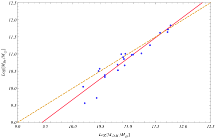
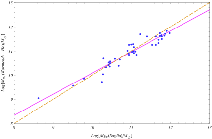
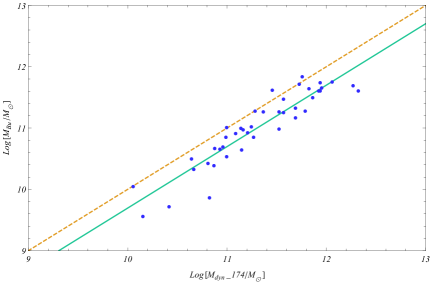
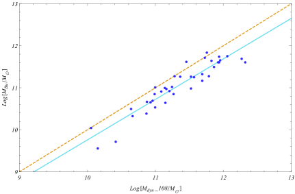
(a) KormendyHo-Cappellari with OLS fitted line ;
(b) KormendyHo-Saglia with OLS fitted line ;
(c) KormendyHo-van den Bosch_174 with OLS fitted line and
(d) KormendyHo-van den Bosch_108 with OLS fitted line .
6 Residual analysis
In Sect. 4 we focused on the role of residual analysis as discussed in Barausse et al. (2017) and Shankar et al. (2019) and highlighted its fundamental statistical aspects.
In Barausse et al. (2017) and Shankar et al. (2019) the interest was in studying correlations between the residuals from various scaling relations as an efficient way of comparing the relative importance of velocity dispersion and the mass of the galaxy . Along the same line, here we consider the role played by and velocity dispersion. In light of the comments in Sect. 4, we first prefer to discuss again the results from Shankar et al. (2019) in Subsect. 6.1 and then to investigate the relative importance of the kinetic energy, characterizing the scaling relation (Feoli and Mele, 2005, 2007; Feoli and Mancini, 2009; Feoli, 2014), compared to the velocity dispersion in Subsect. 6.2.
6.1 Mass of the galaxy and velocity dispersion
The entries in Table 3 give conditional correlations along with confidence intervals. Let , , . In all considered samples, but the first van de Bosch sample, the complete model, with both variables and improves over the model with only one of them. In the first van de Bosch’s sample, the velocity dispersion alone suffices to explain the SMBH. As a general result, velocity dispersion always shows a larger relative importance with respect to the mass of the galaxy, even if evidence of such superiority (at a significance level) can be found only in the first van de Bosch’s sample.
6.2 Kinetic energy and velocity dispersion
The results concerning the analysis of correlations among residuals from scaling relations when the kinetic energy is considered in place of the mass of the galaxy are presented in Table 3, whereas those about the reduction in the sum of squared errors are in Table 4.
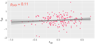
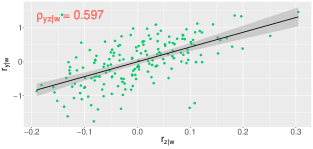
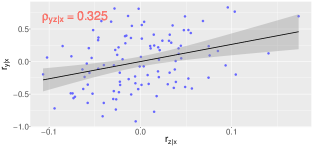
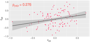
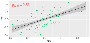
There is no evidence of any significant difference between the magnitude of the correlations coefficients for all the samples except for the first van de Bosch’s sample. Then, with the exception of the latter sample, we notice that, the importance of kinetic energy is larger, even if not significant, than that of velocity dispersion. In contrast, in Subsect. 6.1 we stated that there was no ambiguity about the preeminent role of velocity dispersion over the mass of the galaxy. Moreover, the introduction of the kinetic energy in addition to dispersion velocity improves goodness of fit since it leads to a significant reduction in the sum of squared errors, still with the exception of the first van de Bosch’s sample. The conditional correlations are always larger than the conditional correlations , where . This means that kinetic energy has larger predictive power than the mass of the galaxy. It is worth noting that if is fixed, and are statistically the same. As a result, and this leads us to insert only three subfigures for each figure (Figs. 2 7).
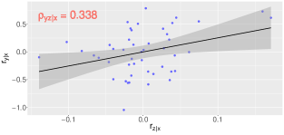
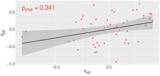
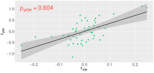
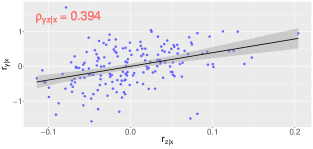
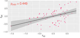
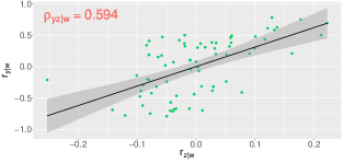
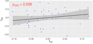
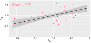
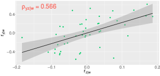
Figures from 2 to 7 allow a visual inspection of conditional correlations among residuals from scaling relations. The fitted lines pass through the origin since the sets of residuals have null mean. The steeper the line the larger the linear correlation. The shaded area can be interpreted as a tolerance region that gives confidence intervals around the fitted line in a pointwise fashion. In general, based on the fitted model (4), confidence intervals around the fitted line are obtained as , , where is the level quantile of the distribution and is the standard error associated to the fitted value . Let be the design matrix, with . The fitted variance-covariance matrix of is . Then, , with . When the shaded area covers entirely the abscissa axis, as in the right panels of Fig. 3, it means there is not any evidence of correlation.
| Sample | Cond. correl | CI | |
|---|---|---|---|
| Cappellari | 0.604 | 0.384 0.760 | |
| 0.338 | 0.056 0.570 | ||
| 0.341 | 0.059 0.572 | ||
| van den Bosch_174 | 0.597 | 0.492 0.685 | |
| 0.394 | 0.260 0.512 | ||
| 0.110 | -0.040 0.254 | ||
| van den Bosch_108 | 0.560 | 0.415 0.678 | |
| 0.325 | 0.145 0.484 | ||
| 0.276 | 0.092 0.442 | ||
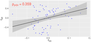
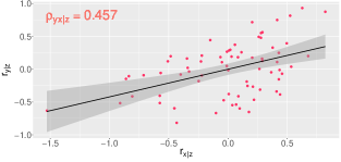
| De Nicola-Saglia | 0.587 | 0.409 0.721 | |
| 0.359 | 0.138 0.547 | ||
| 0.457 | 0.251 0.624 | ||
| Saglia | 0.593 | 0.419 0.727 | |
| 0.370 | 0.150 0.555 | ||
| 0.449 | 0.241 0.618 | ||
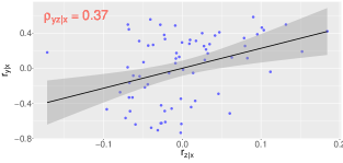
| Kormendy-Ho | 0.566 | 0.327 0.737 | |
| 0.208 | -0.092 0.472 | ||
| 0.576 | 0.340 0.744 | ||
The detailed results for each sample are given below.
-
Cappellari. The entries in Table 3 and Fig. 2 show that there is no evidence of any difference between the magnitude of the two correlations coefficients. According to Table 4, we have that both variables provide a significant reduction at a significance level not lower than about . In summary, in this case, both and share a close relative importance.
-
van den Bosch_174. From the inspection of conditional correlations in Table 3 and Fig. 3, we have that kinetic energy is not significantly correlated with black hole mass given dispersion velocity, whereas there is evidence of a moderate conditional correlation between black hole mass and dispersion velocity given kinetic energy. The analysis in Table 4 confirms that kinetic energy is less important than the dispersion of velocity, whereas, in contrast, the inclusion of velocity dispersion improves significantly over the relation.
-
van den Bosch_108. From the inspection of conditional correlations in Table 3 and Fig. 4, we have that the relative importance of kinetic energy is lower than velocity dispersion, whereas there isn’t evidence of a difference in conditional correlations. The analysis in Table 4 confirms that kinetic energy has a slightly lower importance, since it determines a smaller, but significant still, reduction in the sum of squares. Here, the two explanatory variables under study can be claimed to be equivalent even if gives a slightly larger contribute.
-
de Nicola - Saglia. From the inspection of conditional correlations in Table 3 and Fig. 5, we have that the relative importance of kinetic energy is larger than velocity dispersion, whereas there isn’t evidence of a difference in conditional correlations. The analysis in Table 4 confirms that kinetic energy has a slightly larger importance, since it determines a larger significant reduction in the sum of squares.
-
Saglia. From the inspection of conditional correlations in Table 3 and Fig. 6, we have, the velocity dispersion exhibits a larger conditional correlation with the mass of SMBH, but there is no evidence of a significant difference with the conditional between black hole mass and kinetic energy at a significance level. The reduction in the residual sum of squares is given in Table 4. The introduction of kinetic energy improves the relation with a larger reduction.
-
6th Sample: Kormendy-Ho. From the inspection of conditional correlations in Table 3 and Fig. 7, we can note that there is evidence of a larger conditional correlation between black hole mass and kinetic energy given dispersion velocity, while velocity dispersion is not significantly correlated with black hole mass given the kinetic energy. From the values that we can observe in Table 4, it is possible to note that kinetic energy is more important than the velocity dispersion and improves significantly over the relation.
| Sample | p-value | ||
|---|---|---|---|
| Cappellari | 0.893 | 0.0205 | |
| 0.877 | 0.0216 | ||
| van den Bosch_174 | 0.573 | 0.151 | |
| 8.629 | 0.001 | ||
| van den Bosch_108 | 1.399 | 0.004 | |
| 2.002 | 0.001 | ||
| De Nicola-Saglia | 2.373 | 0.001 | |
| 1.331 | 0.002 | ||
| Saglia | 2.315 | 0.001 | |
| 1.452 | 0.002 | ||
| Kormendy- Ho | 1.532 | 0.001 | |
| 0.139 | 0.177 |
7 Conclusions
In this paper we shed more light on the role played by the single variables in the study of scaling relations and on the correct interpretation of some common statistical analyses. In addition, we investigated the considered scaling relations not only from a goodness of fit point of view but also under a predictive perspective. We have compared the performance of two well known relations the and the . It has been shown that both relations work satisfactory with all the six samples analyzed in this paper. In particular with the samples one, three, four and five the behavior of the two relations can be considered almost equivalent, while with the sample two the first law leads to better results and with sample six the opposite occurs. The comparison from a predictive point of view gives more relevance to the reliability of the relation and the residual analysis did not unveil any substantial preference of one variable, the kinetic energy, over another, the velocity dispersion. It is worth noting that simple scaling relations may be significantly improved by considering a suitably chosen extra variable, for instance introducing the kinetic energy in the , while the same does not occur considering the mass of the galaxy as the extra parameter, in agreement with previous work.
Acknowledgements
This research was partially supported by FAR fund of the University of Sannio.

References
- Aller and Richstone (2007) Aller, M. C., Richstone, D. O.: Astrophys. J., 665, 120 (2007)
- Barausse et al. (2017) Barausse, E., Shankar, F., Bernardi, M., et al.: Mon. Not. R. Astron. Soc., 3468, 4782 (2017)
- Beltramonte et al. (2019) Beltramonte, T., Benedetto, E., Feoli, A., et al.: Astrophys. Space Sci., 364, 212 (2019)
- Benedetto et al. (2013) Benedetto, E., Fallarino, M.T., Feoli, A.: Astron. Astrophys., 558, A108 (2013)
- Bernardi et al. (2003) Bernardi, M., Sheth, R.K., Annis, J., et al.: Astron. J., 125, 1849 (2003)
- Bernardi et al. (2007) Bernardi, M., Hyde, J.B., Sheth, R.K., et al.: Astron. J., 133, 1741 (2007)
- Berrier et al. (2013) Berrier, J.C., Davis, B.L., Kennefick, D., et al.: Astrophys. J., 769, 132 (2013)
- Burkert and Tremaine (2010) Burkert, A., Tremaine, S.: Astrophys. J., 720, 516 (2010)
- Cappellari et al. (2006) Cappellari, M., Bacon, R., Bureau, M., et al.: Mon. Not. R. Astron. Soc., 366, 1126 (2006)
- Cappellari et al. (2013) Cappellari, M., Scott, N., Alatalo, K., et al.: Mon. Not. R. Astron. Soc., 432, 1709 (2013)
- de Nicola et al. (2019) de Nicola, S., Marconi, A., Longo, G.: Mon. Not. R. Astron. Soc., 490, 600 (2019)
- Feoli (2014) Feoli, A.: Astrophys. J., 784, 34 (2014) and references therein
- Feoli and Mancini (2009) Feoli, A., Mancini, L.: Astrophys. J., 703, 1502 (2009)
- Feoli and Mele (2005) Feoli, A., Mele, D.: Int. Jour. Mod. Phys. D, 14, 1861 (2005)
- Feoli and Mele (2007) Feoli, A., Mele, D.: Int. Jour. Mod. Phys. D, 16, 1261 (2007)
- Ferrarese and Ford (2005) Ferrarese, L., Ford, H. C.: Space Sci. Rev., 116, 523 (2005)
- Ferrarese and Merritt (2000) Ferrarese, L., Merritt, D.: Astrophys. J., 539, L9 (2000)
- Gebhardt et al. (2000) Gebhardt, K., Bender, R., Bower, G., et al.: Astrophys. J., 539, 13 (2000)
- Gebhardt et al. (2003) Gebhardt, K., Richstone, D., Tremaine, S., et al.: Astrophys. J., 583, 92 (2003)
- Graham et al. (2001) Graham, A. W., Erwin, P., Caon, N., Trujillo, I.: Astrophys. J., 563, L11 (2001)
- Graham and Driver (2005) Graham, A. W., Driver, S. P.: Proc. Astron. Soc. Aust., 22, 118 (2005)
- Graham and Driver (2007) Graham, A. W., Driver, S. P.: Astrophys. J., 655, 77 (2007)
- Gültekin et al. (2009) Gültekin, K., Richstone, D. O., Gebhardt, K., et al.: Astrophys. J., 698, 198 (2009)
- Häring and Rix (2004) Häring, N., Rix, H.: Astrophys. J., 604, L89 (2004)
- Ho (2004) Ho, L. C.: “Coevolution of Black Holes and Galaxies”, (Carnegie Observatories Astrophys. Series, Vol. 1, Cambridge Univ. Press) (ed. 2004)
- Hopkins et al. (2007a) Hopkins, P. F., Hernquist, L., Cox, T. J., et al.: Astrophys. J., 669, 45 (2007a)
- Hopkins et al. (2007b) Hopkins, P. F., Hernquist, L., Cox, T. J., et al.: Astrophys. J., 669, 67 (2007b)
- Iannella and Feoli (2020) Iannella, A. L., Feoli: Astrophys. Space Sci., 365, 162 (2020)
- Kelly (2007) Kelly, B. C.: Astrophys. J., 665, 1489 (2007)
- Kormendy and Richstone (1995) Kormendy, J., Richstone, D.: Annu. Rev. Astron. Astrophys., 33, 581 (1995)
- Kormendy and Ho (2013) Kormendy, J., Ho, L.C.: Annu. Rev. Astron. Astrophys., 51, 511 (2013)
- Laor (2001) Laor, A.: Astrophys. J., 553, 677 (2001)
- Lauer et al. (2007) Lauer, T. R., Faber, S. M., Richstone, D.: Astrophys. J., 662, 808 (2007)
- Magorrian et al. (1998) Magorrian, J., Tremaine, S., Richstone, D., et al.: Astron. J., 115, 2285 (1998)
- Mancini and Feoli (2012) Mancini, L., Feoli, A.: Astron. Astrophys., 537, A48 (2012)
- Marconi et al. (2001) Marconi, A., Capetti, A., Axon, D. J., et al.: Astrophys. J., 549, 915 (2001)
- Marconi and Hunt (2003) Marconi, A., Hunt, L. K.: Astrophys. J., 589, L21 (2003)
- Merritt and Ferrarese (2001) Merritt, D., Ferrarese, L.: ASP Conf. Proc. 249, The Central Kiloparsec of Starbursts and AGN: The La Palma Connection, ed. J.H. Knapen, J.E. Beckman, I. Shlosman, T.J. Mahoney, (San Francisco, CA: ASP), 335 (2001)
- Richstone et al. (1998) Richstone, D., Ajhar, E. A., Bender, R., et al.: Nature, 395, A14 (1998)
- Saglia et al. (2016) Saglia, R. P., Opitsch, M., Erwin, P., et al.: Astrophys. J., 818, 47 (2016)
- Seigar et al. (2008) Seigar, M. S., Kennefick, D., Kennefick, J., et al.: Astrophys. J., 683, L211 (2008)
- Shankar et al. (2016) Shankar, F., Bernardi, M., Sheth, R.K.,et al.: Mon. Not. R. Astron. Soc., 460, 3119 (2016)
- Shankar et al. (2017) Shankar, F., Bernardi, M., Sheth, R.K.: Mon. Not. R. Astron. Soc., 466, 4029 (2017)
- Shankar et al. (2019) Shankar, F., Bernardi, M., Richardson, K.,et al.: Mon. Not. R. Astron. Soc., 485, 1278 (2019)
- Snyder et al. (2011) Snyder, G. F., Hopkins, P. F., Hernquist, L.: Astrophys. J., 728, L24 (2011)
- Soker and Meiron (2011) Soker, N., Meiron, Y.: Mon. Not. R. Astron. Soc., 411, 1803 (2011)
- Stock and Watson (2015) Stock, J.H., Watson, M.W.: Introduction to Econometrics, 3rd edn. p. 215 Pearson, New Jersey (2015)
- The Event Horizon Telescope Collaboration (2019) The Event Horizon Telescope Collaboration: Astrophys. J. Lett., 875, L6 (2019)
- Tremaine et al. (2002) Tremaine, S., Gebhardt, K., Bender, R., et al.: Astrophys. J., 574, 740 (2002)
- van den Bosch (2016) van den Bosch, R. C. E.: Astrophys. J., 831, 134 (2016)
- van der Marel (1999) van der Marel, R. P.: Astron. J., 117, 744 (1999)
- Wandel (2002) Wandel, A.: Astrophys. J., 565, 762 (2002)