Chandra/LETGS Studies of the Collisional Plasma in 4U 1626$-$67

Abstract

We present an analysis of Chandra/LETGS observations of the ultracompact X-ray binary (UCXB) 4U 1626$-$67 (catalog 4U 1626$-$67), continuing our project to analyze the existing Chandra gratings data of this interesting source. The extremely low mass, hydrogen-depleted donor star provides a unique opportunity to study the properties and structure of the metal-rich accreted plasma. There are strong, double-peaked emission features of O VII–VIII and Ne IX–X, but no other identified emission lines are detected. Our spectral fit simultaneously models the emission line profiles and the plasma parameters, using a two-temperature collisionally-ionized plasma. Based on our line profile fitting, we constrain the inclination of the system to 25–60^∘ and the inner disk radius to $\sim$1500 gravitational radii, in turn constraining the donor mass to $\lesssim$0.026 $M_{\odot}$, while our plasma modeling confirms previous reports of high neon abundance in the source, establishing a Ne/O ratio in the system of $0.47\pm 0.04$, while simultaneously estimating a very low Fe/O ratio of $0.0042\pm 0.0008$ and limiting the Mg/O ratio to less than 1% by number. We discuss these results in light of previous work.

=20

1 Introduction

4U 1626$-$67 is an ultracompact X-ray binary (UCXB), featuring a neutron star in a 42-minute orbit around a very low-mass companion, and is unique as the only UCXB hosting a persistent X-ray pulsar. The source was discovered by Uhuru (Giacconi et al., 1972), with 7.68 s pulsations discovered in SAS-3 data by Rappaport et al. (1977). A faint, blue star was suggested for the companion by McClintock et al. (1977), confirmed by the observation of optical pulsations at the X-ray period by Ilovaisky, Motch & Chevalier (1978). A highly compact binary orbit with a low-mass companion was first suggested by Joss, Avni & Rappaport (1978), based on the lack of significant timing residuals in the X-ray band. The compactness of the orbit was more firmly established by Middleditch et al. (1981), who identified the 42 min orbital period in the optical pulsations; this was later confirmed by Chakrabarty (1998). A cyclotron resonance scattering feature (CRSF) was discovered at $\sim$37 keV in BeppoSAX data by Orlandini et al. (1998), implying a magnetic field strength of $\sim$4.2$\times 10^{12}$ G.

The X-ray pulsar was in a spin-up state with a timescale of $\sim$5000 yr for several decades until 1990, after which CGRO/BATSE observations revealed that the source had transitioned to a spin-down state (see Chakrabarty et al., 1997, and references therein). The source’s X-ray luminosity had also been declining steadily since its discovery, which lead Krauss et al. (2007) to predict that the source would fade into quiescence in a few years. However, both of these trends were reversed with a second torque reversal in 2008 (Camero-Arranz et al., 2010), which was accompanied by a large increase in X-ray flux (Camero-Arranz et al., 2012), bringing the source back to its pre-1990 brightness.

The nature of the donor star in 4U 1626$-$67 is uncertain. Based on the small semimajor axis ($a\sin i\lesssim 8$ lt-ms, per Shinoda et al., 1990) and the requirement that the donor fill its Roche lobe, Verbunt, Wijers & Burm (1990) and Chakrabarty (1998) proposed that the donor was either a helium-burning star of mass $\sim$0.6 $M_{\odot}$, a partially-degenerate, H-poor $\sim$0.08 $M_{\odot}$ star, or a white dwarf (WD) of mass $\sim$0.02 $M_{\odot}$. The low-mass white dwarf case is currently favored, as it imposes less stringent limits on inclination ($\lesssim 33^{\circ}$) and is easier to reconcile with the system’s overall faintness in the optical, blue color, and the lack of detected hydrogen and helium lines in the system (Homer et al., 2002; Werner et al., 2006).

The X-ray spectrum from 4U 1626$-$67 is complex and somewhat peculiar, made only more so by the advent of high-resolution spectroscopy. A complex of emission lines around 1 keV were first observed by Angelini et al. (1995) using ASCA; they found anomalously high flux from Ne X (the first hint of enhanced neon abundance in the system), along with emission from O VIII. High-resolution X-ray spectra from Chandra and XMM-Newton (Schulz et al., 2001; Krauss et al., 2007) resolved the broad Ne X and O VIII features into double-peaked lines, suggesting an accretion disk origin, as well as finding and characterizing the Ne IX and O VII emission. The only other detected emission feature in 4U 1626$-$67 is a weak iron line complex around 6.4 keV (Camero-Arranz et al., 2012). The 2006 Suzaku and 2010 Chandra/HETGS observations report a near-neutral iron fluorescence line at $\sim$6.4 keV, while the 2010 Suzaku observation and 2015 NuSTAR observations see a 6.7 keV feature but no evidence for the neutral line (Camero-Arranz et al., 2012; Koliopanos & Gilfanov, 2016; D’Aì et al., 2017; Schulz, Chakrabarty & Marshall, 2019). It remains unclear why the iron complex appears as different as it does between these studies — there were only $\sim$9 months between the 2010 Chandra and Suzaku observations. Meanwhile, the optical (Werner et al., 2006; Nelemans, Jonker & Steeghs, 2006) and UV (Homer et al., 2002) spectra show a complete lack of lines from hydrogen, helium, and nitrogen, while finding excess emission from oxygen and some hints of extra carbon in the system. Oddly, Werner et al. (2006) also do not detect any neon lines, placing an upper limit on the neon abundance of $\sim$10% solar, in conflict with the enhanced neon abundance implied by the X-ray data.

The low flux of 4U 1626$-$67 in the early 2000s hindered early efforts to carry out detailed high-resolution studies of the lines. Fortunately, the 2008 torque reversal was accompanied by a disproportionately large increase in the line flux, with the lines brightening by a factor of $\sim$8 (compared to $\sim$3 for the continuum, as shown using Suzaku observations bracketing the reversal by Camero-Arranz et al., 2012). This has enabled Schulz, Chakrabarty & Marshall (2019) to carry out a detailed study of the post-torque reversal Chandra/HETGS observations, and to compare those results with the pre-reversal HETGS data. Their work settles on a two-temperature, collisionally-ionized plasma in the disk as the origin of the strong emission lines. If the lines trace the inner edge of the disk, the pre- and post-torque-reversal Chandra observations imply that the disk moved inwards, consistent with the transition to spin-up.

Continuing these efforts to comprehensively analyze the high-resolution spectra of 4U 1626$-$67, this paper investigates Chandra/LETGS observations of 4U 1626$-$67 made in 2014, during the source’s post-reversal era. Here, we will extend the work of Schulz, Chakrabarty & Marshall (2019) by implementing a properly disk-blurred plasma model, unlike the simpler red- and blue-shifted plasma models in the previous paper, allowing us to simultaneously model the kinematic and plasma parameters of the accretion disk. We present an overview of the data and the extraction in Section 2. The lightcurves, pulse period evolution, and pulse profiles are addressed in Section 2.1. The bulk of the study is the spectral modeling in Section 3, particularly the modeling of the prominent emission lines in 4U 1626$-$67’s spectrum in Section 3.2, 3.3, and 3.4. We discuss the results of these fits and their interpretation in Section 4, and summarize the results and compare with other work in Section 5.

2 Observations and Data Reduction

Chandra has observed 4U 1626$-$67 multiple times over its mission. In this work, we focus on Chandra ObsIDs 16636, 15765, and 16637, taken in 2014 between July 8 and 13. These observations use the Low-Energy Transmission Grating Spectrometer (LETGS; Brinkman et al., 2000), which uses the Low Energy Transmission Gratings (LETG) to disperse X-rays onto the High-Resolution Camera (HRC). These observations are summarized in Table 1 and represent a total exposure of 131.9 ks. We extracted spectra and lightcurves using the CIAO Fruscione et al. (2006) v4.9, via the Transmission Grating Catalog and Archive software (TGCat; Huenemoerder et al., 2011). Since the HRC has no energy resolution, all orders are combined in a single spectrum for each grating arm. We load ancillary response files (ARFs) and response matrices (RMFs) through eighth order when analyzing these spectra. The CALDB version was 4.7.6, although we also applied an updated degapping file for the HRC, as otherwise there is a systematic wavelength offset between the positive and negative-order spectra. All extractions and analysis were carried out using version 1.6.2-40 of the Interactive Spectral Interpretation System (ISIS; Houck & Denicola, 2000). Unless otherwise stated, all uncertainties are reported at the 90% level.

Table 1: Summary of Chandra/LETGS observations of 4U 1626$-$67

ObsID	Observation start		Exposure	Average countrate
	Date	MJD	ks
16636	2014 July 8	56846.66	$23.0$	$3.21$
15765	2014 July 11	56846.05	$59.4$	$3.66$
16637	2014 July 13	56846.80	$49.5$	$3.65$

2.1 Lightcurves and Timing Analysis

We extracted lightcurves for the full LETGS band and for the 0.2–2 and 2–8 keV bands with 0.5 s time resolution. The full-band lightcurves of the three observations are plotted in Figure 1. Between the first and second observation (ObsIDs 16636 and 15765, respectively), the flux increased by $\sim$15%. Variability changes are also clearly visible in the lightcurves, with the first exhibiting considerably more high-amplitude short-term variability than the later two, and two (or three) large flares in the last observation.

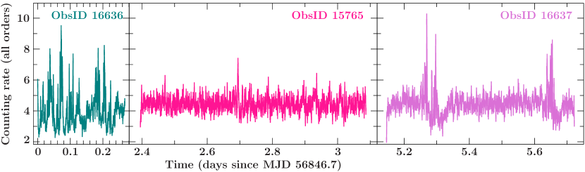
Figure 1: The lightcurves of the three Chandra/LETGS observations of 4U 1626$-$67, binned at $76.7$ s (ten times the pulse period). The plots are scaled to the durations of the observations and are displayed relative to the start time of ObsID 16636.

After barycentering the lightcurve, a first estimate of the pulse period was determined via epoch folding (Leahy et al., 1983). A pulse period determined from epoch folding can be refined by comparing individual pulses at this period to a reference pulse profile, typically of the full observation. The phase shifts between the individual pulses and reference profile, $\delta\varphi$, are related to a correction to the assumed pulse frequency, $\delta\nu$, and the rate of change of the pulse period, $\dot{\nu}$, via

$$\delta\varphi\left(t\right)=\varphi_{0}+\delta\nu\left(t-t_{0}\right)+\frac{1}{2}\dot{\nu}\left(t-t_{0}\right)^{2},$$ (1)

where $t_{0}$ is some reference time and $\varphi_{0}$ is the phase offset at $t=t_{0}$. This allows one to correct the original estimate for the pulse frequency, and the procedure is repeated until it converges (this typically only takes a few iterations). The LETGS lightcurves do not have enough counts to do this on a pulse-by-pulse basis, so we produced average pulse profiles by adding up every 200 pulses based on the period derived from epoch folding, and found phase shifts by cross-correlating with the average pulse profile from the entire LETGS lightcurve. The phase shifts are nearly linear and the procedure outlined above converges after only a single iteration. The final pulse period we obtain is $7.67375(7)$ s, consistent with the pulse period obtained by Fermi/GBM during this time period (Camero-Arranz et al., 2010), as shown in Figure 2. The short time spanned by the LETGS observations means $\dot{\nu}$ cannot be meaningfully constrained, but our results are consistent with the decline of $\sim$0.001 s yr^-1 from the Fermi measurements.

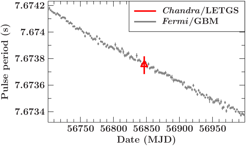
Figure 2: The pulse period determined from the Chandra/LETGS, overplotted with the pulse periods measured by the Fermi/GBM.

Folding the observations’ lightcurves on the measured pulse period obtains the pulse profiles displayed in Figure 3. The pulse profile changes from a single broad peak at low energies to a pair of narrow peaks close together in phase above 2 keV. This may be indicative of a switch from a fan beam at low energies to a pencil beam at higher energies (Pottschmidt et al., 2018). These profiles are qualitatively very similar to those presented in Beri, Paul & Dewangan (2015).

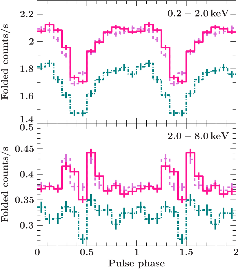
Figure 3: The pulse profiles for 4U 1626$-$67 in the 0.2–2 (top) and 2–8 keV (bottom) bands. ObsID 16626 is the teal dash-dotted line, while 15765 and 16637 are the solid pink and dashed violet lines, respectively. The dramatic change in shape, from a broad single peak to a pair of close, narrow peaks is characteristic of this source. The count rate is low in the 2–8 keV profile mainly due to the LETGS’ low effective area at higher energies.

3 Spectral analysis

The LETGS spectra show unambiguous emission features around $12$, $13$, $19$, and $21$ Å, which we identify as emission from Ne X, Ne IX, O VIII, and O VII, respectively. Their higher-order counterparts are also visible, with the most obvious higher-order feature being the third-order Ne X line appearing at $\sim$36.5 Å. The features, especially the hydrogen-like lines, have clear double-peaked profiles and similar widths. Fitting the hydrogen-like lines with a pair of Gaussians in the manner of Krauss et al. (2007), tying the velocity shifts of the red and blue peaks together, the Ne X peaks are shifted relative to their rest wavelength by $2370\pm 90$ km s^-1, and the O VIII line peaks are shifted by $2360\pm 140$ km s^-1. These are moderately wider separations than were measured by Krauss et al. (2007) and consistent with Schulz, Chakrabarty & Marshall (2019)’s conclusion that the line-producing region has moved inwards since the 2008 torque reversal. Figure 4 displays the Ne X and O VIII profiles on a common velocity axis. Interestingly, despite the presence of carbon in the UV and optical spectra (Homer et al., 2002; Werner et al., 2006), no emission from C VI (33.74 Å) or C V (40.73–41.472 Å) is visible. The apparent lack of carbon may be due to high temperatures in the disk — this is discussed in more detail in Section 4.2.1. The only other immediately apparent feature is an emission feature at $\sim$17 Å, which we model in this work with a Gaussian. This feature’s identity is not immediately apparent — see Section 4.2.2 for a more in-depth discussion.

In the following spectral analysis, unless otherwise noted, we bin the LETGS spectra to a minimum of 2 channels per bin and a minimum signal-to-noise of 8, only using data between 2 and 60 Å. We use $\chi^{2}$ statistics when fitting, as with this binning the spectra generally have significantly more than 20 counts per bin.

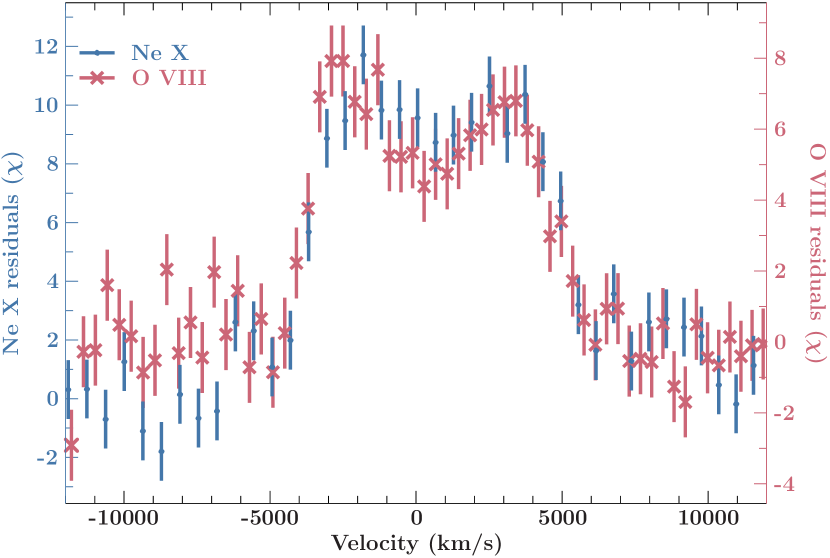
Figure 4: The first-order Ne X (blue points) and O VIII (red crosses) line profiles as seen in ObsIDs 15765 and 16637. We plot here the residuals after both grating arms have been combined and the continuum has been subtracted off, placed on a common velocity axis relative to the literature values (Erickson, 1977) for the K$\alpha$ transition for H-like Ne and O. The double-peaked nature of the lines is clearly visible, and both features show very similar profiles and velocity widths. Note the different scales for the lines — the Ne X profile follows the left y-axis scale, and the O VIII line follows the right y-axis. Also note that the LETGS spectra also have the higher-order counterparts to these lines (not plotted), which have accordingly higher spectral resolution.

3.1 Spectral continuum

To establish a spectral model for the continuum, we fitted the combined spectra from both grating arms, excising data within 0.5 Å of the Ne IX–X and O VII–VIII lines (and their higher-order counterparts). The continuum model chosen is the same as has been used in the past for this source: an absorbed $\Gamma\sim 1$ power law plus a $\sim$0.5 keV black body. For broad-band absorption, we use TBabs, an updated version of the tbabs absorption model of Wilms, Allen & McCray (2000), from which we also take our ISM abundances. The cross-sections are taken from Verner et al. (1996). The best-fit parameters for each ObsID can be found in Table 3.1.

While there are obvious changes in flux and spectral shape between these three ObsIDs (most obviously between the first and second observations), these differences are not straightforwardly reflected in the best-fit spectral parameters — all parameters are consistent with each other within their 90% uncertainties. We thus carried out a set of Markov Chain Monte Carlo (MCMC) runs to obtain the approximate probability distribution of the parameter space, using an ISIS implementation of the emcee algorithm (produced by M. Nowak, based on Foreman-Mackey et al., 2013). Each dataset was run separately with 100 walkers and a chain length of 5000. The walkers generally settled to their most-probable values within $\sim$500 steps, so in our analysis we discard the first 10% of each chain.

In Figure 5, we plot the two-dimensional 95% probability contours for the power law and blackbody parameters from the MCMC runs. Strong degeneracies between these parameters result in the large single-parameter uncertainties and formal consistency between the datasets that were seen in the spectral fits. However, the MCMC results also reveal a clear inconsistency in the power law normalization between the first and the later observations. Thus, a change in the power law normalization (perhaps due to a change in the accretion rate) appears to be the driver of the change in flux between the observations. Additionally, despite the overlap in the contours, it is interesting to note that the positive correlation between the blackbody temperature and area between the observations runs counter to the long-term inverse correlation seen in the post-torque-reversal HETGS data (Schulz, Chakrabarty & Marshall, 2019).

We also find a significantly higher $N_{\mathrm{H}}$ compared to previous studies ($\sim 1.7\times 10^{21}$ cm^-2, compared to the $\sim 1.4\times 10^{21}$ cm^-1 reported by Krauss et al., 2007)), and a moderately softer photon index ($\sim$1.4, compared to $\sim$1.2 in Schulz, Chakrabarty & Marshall, 2019). However, our MCMC runs find strong degeneracy between $N_{\mathrm{H}}$ and $\Gamma$, and the 95% confidence contours are consistent with the values of $N_{\mathrm{H}}$ and $\Gamma$ found by Schulz, Chakrabarty & Marshall (2019) using HETGS data. Further fits with $N_{\mathrm{H}}$ fixed to $1.4\times 10^{21}$ cm^-2 bear this out, finding values more consistent with previous studies.

The absorption edges of the main elements in question in this study (C, O, Ne, Mg, and Fe; see Section 4.3) do not appear to be overly strong in the LETGS spectra. Fitting with a variable-abundance absorption model (TBvarabs) and allowing these abundances to vary, the oxygen, carbon, and magnesium abundances derived from the line-of-sight absorption are consistent with their ISM values, although only oxygen is well-constrained. For carbon the poor constraint may be related to the fact that the carbon K edge at 43.6 Å is coincident with the O VII line in the second order. Neon and iron are moderately underabundant, with 90% upper limits of $0.55$ and $0.75$ relative to the ISM values.

Table 2: Continuum spectral parameters for 4U 1626$-$67, excluding spectral lines. The source distance is assumed to be 5 kpc (Schulz, Chakrabarty & Marshall (2019))

	16636	15765	16637
$N_{\rm H}$ ($\times 10^{22}$ cm-2)	$0.173\pm 0.018$	$0.191\pm 0.020$	$0.177\pm 0.018$
$A_{\rm PL}$ ($\times 10^{-2}$ ph cm-2 s-1)	$4.3\pm 0.5$	$5.5\pm 0.6$	$5.1\pm 0.6$
$\Gamma$	$1.31\pm 0.14$	$1.38\pm 0.14$	$1.32\pm 0.14$
$A_{\rm BB}$ ($R_{\rm km}^{2}/D_{10}^{2}$)	$114\pm 12$	$118\pm 12$	$123\pm 13$
$kT_{\rm BB}$ (keV)	$0.45\pm 0.05$	$0.49\pm 0.05$	$0.48\pm 0.05$
$\lambda_{\rm gauss}$ (Å)	$16.8\pm 1.7$	$16.9\pm 1.7$	$16.9\pm 1.7$
$\sigma_{\rm gauss}$ (Å)	$0.215\pm 0.022$	$0.210\pm 0.021$	$0.256\pm 0.026$
$A_{\rm gauss}$ ($\times 10^{-4}$ ph cm-2 s-1)	$5.9\pm 0.6$	$6.0\pm 0.7$	$7.3\pm 0.8$
$F_{0.5\text{--}10{\rm keV}}$ ($\times 10^{-10}$ erg cm-2 s-1)	$4.63$	$5.47$	$5.52$
$L_{0.5\text{--}10{\rm keV}}$ ($\times 10^{36}$ erg s-1)	$1.38$	$1.64$	$1.65$

Figure 5: The MCMC-derived 2-dimensional contours for the power law normalization vs. power law index (left) and the blackbody temperature vs. normalization (right). The contours represent the 68% and 95% confidence limits. The power law normalizations are inconsistent between the first observation (ObsID 16636, teal) and the final two (ObsIDs 15765 and 16637, magenta and pink, respectively), while there is a sizable overlap in the blackbody parameters.

3.2 Diskline modeling

Building on the work in Schulz, Chakrabarty & Marshall (2019), we present here a detailed analysis of of the double-peaked emission lines. As in Schulz, Chakrabarty & Marshall, we model the Ne IX–X and O VII–VIII lines with the diskline model (Fabian et al., 1989), fixing the emissivity power-law index $q$ to $-3.6$, the same value used for the HETGS data. This large negative value for $q$ (i.e., line emission falling off quickly with radius) is justified by the clear trough between the line peaks in both the Ne X and O VIII profiles: if there were significant emission from the outer disk (i.e., $q$ closer to zero), it would fill in the space between the peaks.

We obtained a first set of fits using only the Ne X and O VIII features, as they are bright and, unlike the He-like triplets, they are not blended with other features. We performed simultaneous local fits to the Ne and O features, using the best-fit continuum from Section 3.1 and noticing only the 11–13 Å and 18–20 Å regions of the spectra. We initially fit with the inner and outer disk radii ($R_{\rm in}$ and $R_{\rm out}$) free to vary between the lines and between observations, while the inclination was tied between all components. The inner disk radius was consistent between all ObsIDs and between the Ne X and O VIII lines, at roughly 1000–1500 $GM/c^{2}$, which for a $1.4$ $M_{\odot}$ neutron star translates to 2–3$\times 10^{8}$ cm. The outer radii were more poorly constrained, which is unsurprising given the steep slope in the emissivity that we assume, but were typically around $10^{4}$ $GM/c^{2}$ ($2\times 10^{9}$ cm), with lower bounds of a few $\times 10^{3}$ $GM/c^{2}$. The line wavelengths are consistent with their rest wavelengths (from Erickson, 1977, via AtomDB), and the oxygen-to-neon flux ratios were $\sim$1.1 in all observations. The full set of best-fit parameters can be found in Table 3.

Table 3: diskline fits to Ne X and O VIII lines

		16636	15765	16637
Emissivity index $q$		$-3.60$
	Inclination (∘)	$34^{+19}_{-10}$
Ne X	Norm ($10^{-3}$ ph cm-2 s-1)	$2.25\pm 0.20$	$2.68\pm 0.14$	$2.72^{+0.16}_{-0.15}$
	Wavelength (Å)	$12.134^{+0.011}_{-0.008}$	$12.135^{+0.009}_{-0.010}$	$12.130^{+0.008}_{-0.010}$
	$R_{\rm in}$ ($10^{3}$ $GM/c^{2}$)	$1.5^{+3.7}_{-0.6}$	$1.4^{+3.4}_{-0.6}$	$1.1^{+3.4}_{-0.5}$
	$R_{\rm out}$ ($10^{3}$ $GM/c^{2}$)	$>2.4$	$10^{+25}_{-6}$	$>3.5$
O VIII	Norm ($10^{-3}$ ph cm-2 s-1)	$2.59\pm 0.30$	$3.08\pm 0.21$	$3.00\pm 0.22$
	Wavelength (Å)	$18.977^{+0.016}_{-0.017}$	$18.980\pm 0.010$	$18.965^{+0.014}_{-0.011}$
	$R_{\rm in}$ ($10^{3}$ $GM/c^{2}$)	$1.4^{+1.0}_{-0.5}$	$1.4^{+3.3}_{-0.5}$	$1.4^{+3.4}_{-0.7}$
	$R_{\rm out}$ ($10^{3}$ $GM/c^{2}$)	$3.3^{+2.5}_{-1.3}$	$4.8^{+7.9}_{-2.2}$	$7^{+21}_{-4}$
	$\chi^{2}_{\nu}$ (dof)	1.22 (443)

Once the disk parameters were established, we fixed their values and expanded the wavelength range and model to include the helium-like triplets. Since there was no detectable shift in the line wavelengths for the H-like features, we fixed the wavelengths of the Ne IX and O VIII lines to their values in AtomDB (Foster et al., 2012), and re-fit to obtain the normalizations of the He-like triplets. The resulting fits are summarized in Table 4 and plotted in Figure 6.

The diskline fits indicate a strong resonance feature compared to the forbidden and intercombination transitions. This is interesting, as visually the triplets, especially Ne IX, appear to be dominated by the intercombination transition (as reported by Schulz et al., 2001; Krauss et al., 2007; Schulz, Chakrabarty & Marshall, 2019). In fact, the velocity splitting of the lines by the disk is coincidentally similar to the separation between the lines in the triplets, and as a result the apparent strong “intercombination” feature seen in the Ne IX triplet is actually the sum of the red wing of the $r$ line and the blue wing of the $f$ line. The $i$ and $f$ transitions are weak and typically more poorly constrained than the $r$ transitions, especially in the oxygen triplet.

To estimate confidence intervals for the $R=f/i$ and $G=(f+i)/r$ ratios, we carried out a set of MCMC runs, with 100 walkers and a chain length of 2000, (this typically converged to the best-fit parameters $\sim$1000 steps, so we discarded the first 50% of the chains). During this process we adjusted the hard limits on the line amplitudes to allow for negative fluxes. The resulting posterior distributions of line normalizations for the $r$, $i$, and $f$ transitions for neon and oxygen were convolved to determine the distributions for $R$ and $G$. We include the maximum a posteriori values and 90% confidence intervals for $R$ and $G$ in Table 4. As can be seen clearly from the confidence intervals, the distributions are highly skewed, typically with long tails at the high end, due to the skewed distributions of the line fluxes themselves. The poor detection of the $i$ and $f$ lines in some of the observations also leads to negative $R$-ratios in some cases, due to the line fluxes being consistent with zero or negative. Nonetheless, the results prefer relatively low values (less than a few) for $R$ and $G$. The $R$-ratio is too poorly determined to offer a meaningful constraint on density (and, in any case, is likely contaminated by UV depopulation from the disk, per Schulz, Chakrabarty & Marshall, 2019), but the moderately low $G$ value found in most of the observations favors the hot, collisionally-ionized plasma inferred by Schulz, Chakrabarty & Marshall (2019) as the origin for the emission.

Figure 6: The Ne IX (left) and O VII (right) triplets, decomposed into, from left to right within each plot, the $r$ (blue), $i$ (green), and $f$ (red) transitions. The gray line shows the total model. For clarity, we show all ObsIDs combined here. The resonance lines are strong in both profiles, dominating the flux of the oxygen triplet, supporting a high-temperature collisional plasma as the nature of the underlying medium.

Table 4: Line normalizations of Ne IX and O VII triplets

	$\lambda$ (Å)	16636	15765	16637
Ne IX $r$	13.447	$0.29\pm 0.21$	$0.22\pm 0.16$	$0.46^{+0.15}_{-0.19}$
$i$	13.5515	$0.30\pm 0.25$	$0.21\pm 0.18$	$<0.276$
$f$	13.699	$0.25\pm 0.19$	$0.29\pm 0.13$	$0.19^{+0.14}_{-0.16}$
$R$	$f/i$	$0.5^{+3.4}_{-0.4}$	$0.9^{+4.3}_{-0.5}$	$0.5^{+6.0}_{-7.0}$
$G$	$(f+i)/r$	$1.3^{+4.5}_{-0.7}$	$1.8^{+4.5}_{-0.9}$	$0.4^{+1.0}_{-0.3}$
O VII $r$	21.602	$0.7\pm 0.5$	$1.3\pm 0.4$	$1.0\pm 0.4$
$i$	21.8025	$0.5\pm 0.5$	$<0.767$	$<0.798$
$f$	22.098	$<0.411$	$<0.486$	$<0.565$
$R$	$f/i$	$-0.1^{+1.8}_{-1.2}$	$0.0^{+3.3}_{-1.5}$	$0.1^{+3.9}_{-2.6}$
$G$	$(f+i)/r$	$0.4^{+2.4}_{-0.4}$	$0.4^{+0.6}_{-0.2}$	$0.5^{+1.0}_{-0.3}$
$\chi^{2}_{\nu}$ (dof)		1.17 (996)

3.3 Plasma modeling

Figure 7: From top to bottom, a two-temperature photoionized plasma with enhanced neon, a single-temperature APEC with standard neon abundance, and a two-temperature APEC with higher neon abundance. Both panels show ObsIDs 15765 and 16637 combined. Enhanced neon abundance is clearly needed to produce the observed Ne-to-O ratio. The photoionized plasma clearly fails to fit the spectrum, with a strong radiative recombination feature from Ne around 9 Å and failing to reproduce the He-like triplets. The single-temperature APEC also fails to reproduce the helium-like oxygen triplet around 22 Å.

Continuing the work of Schulz, Chakrabarty & Marshall (2019), we constructed a set of APEC plasma models (functionally equivalent to XSPEC’s vvapec models). As discussed in Schulz, Chakrabarty & Marshall (2019), the true nature of the plasma in 4U 1626$-$67’s accretion disk is likely much more complicated than APEC can provide on its own — this model is only an approximation. However, we nonetheless find that we achieve a remarkably good reproduction of the observed spectra using this approach.

While the baseline abundances used by the APEC models are the solar abundances of Anders & Grevesse (1989), we vary these quite drastically to obtain a good reproduction of 4U 1626$-$67’s spectrum. First, as in Schulz, Chakrabarty & Marshall (2019), we set the abundances of all elements to zero, other than those of carbon, oxygen, neon, and iron, as only those elements have detected features in the optical, UV, or X-ray spectra (Homer et al., 2002; Werner et al., 2006; Krauss et al., 2007; Camero-Arranz et al., 2012), and the expected donor star is likely depleted in other elements. Additionally, the conventional definition of “abundance” (i.e., measured relative to the hydrogen number density) is inapplicable to the hydrogen-depleted plasma we see in 4U 1626$-$67, so we instead measure abundances relative to oxygen by fixing the oxygen abundance to unity (see Section 4.2.1 for how to interpret the resulting measurements).

Based on the temperature inferred from the $G$-ratio above, we initially tried a 10 MK plasma with red- and blueshifted components. However, this did not fit the data adequately. As can be seen in Figure 7, a single-temperature plasma with a neon abundance set to unity (i.e., a solar Ne/O ratio) fails to fit the relative heights of the neon and oxygen lines, producing too little flux from neon, and it fails to reproduce the helium-like triplets from either element. Allowing the neon abundance to vary, we found that a factor of $\sim$3.5 overabundance of neon successfully reproduced the high Ne X flux and improved the fit to the Ne IX triplet with a , but the O VII triplet could only be fully reproduced by introducing a second, lower-temperature component with $T_{\rm cool}\sim 2$ MK.

At these high temperatures, the carbon lines are intrinsically weak (due to the carbon being almost fully ionized — see Section 4.2.1), and as a result we could not obtain meaningful constraints on the carbon abundance. However, we do find a very low but nonzero iron abundance of $0.025$, mostly constrained by the lack of detected L-shell iron lines in the 15–20 Å range — the only feature in this range is the unidentified 17 Å feature, which this plasma model cannot reproduce without also producing considerably higher-flux iron lines in the 15–16 Å region, which are inconsistent with the data. The LETGS’ sensitivity below a few Å is too low to detect the iron K line, but the upper limits for a line in that region are consistent with the line seen by NuSTAR (D’Aì et al., 2017; Iwakiri et al., 2019).

The inferred turbulent velocities of the two components were $\sim$2200 and $\sim$1500 km s^-1, similar to what was found in the HETGS data; however, it should be noted that this does not take into account any blurring due to the disk. The red- and blueshifts on the 10 MK and 2 MK components were consistent within errors at approximately $\pm 0.008$, suggesting that the two temperature components exist at roughly the same orbital distance from the neutron star. This is reassuring, given our assumptions made when modeling the helium-like lines with diskline above.

3.4 Combined APEC-diskline Modeling

We can improve on our somewhat crude red- and blueshifted APEC model by using diskline profiles for the lines in the APEC model. We accomplish this by convolving the two-temperature APEC with an rdblur model component, which relativistically blurs an arbitrary input spectrum based on the same code as the diskline model. Since our diskline modeling and our initial APEC fits suggest that both temperature components come from approximately the same orbital distance, we use a single rdblur component for both temperatures. As in Section 3.2, we fix $q$ to $-3.6$, but we leave the remaining disk parameters free to vary. Our final best-fit model for 4U 1626$-$67 is thus TBabs(pow+bb+rdblur(apec2)+gauss), where pow is the power law, bb is the blackbody, gauss is the Gaussian at 16.9 Å, and apec2 is a two-temperature APEC model with variable abundances. We allow the power law and blackbody components to vary between the observations, but tie the plasma and disk parameters for all ObsIDs together, as our diskline fits found consistent parameters and line ratios between all observations. As before, we set the abundances of most elements in the APEC plasma to zero — although now in addition to carbon, oxygen, neon, and iron, we also include magnesium, as this would be the next-most abundant element in an oxygen-neon white dwarf, which is one of the possible donor stars in this system.

The best-fitting model is dominated by a $\sim$13 MK component, which produces most of the neon emission and some of the O VIII feature, while a $2.3$ MK component mostly produces the helium-like oxygen lines. The inclusion of the rdblur model simultaneously constrains the accretion disk parameters by modeling the line profiles. These results can be found in Table  5, and the spectrum with the best-fit model is plotted in Figure 8. Zoomed-in plots showing the line regions of interest are plotted in Figure 9. Compared to the unblurred APEC model of Section 3.3, these fits find considerably smaller turbulent velocities, as blurring by the disk accounts for most of the line widths. The disk parameters are largely consistent with what we found fitting the individual lines with diskline.

In terms of chemical abundances, we find similar results to our pure APEC fits: overabundant neon, poorly-constrained carbon, and a small but nonzero iron abundance. The carbon and magnesium abundances are constrained to upper limits of $0.488$ and $0.190$, although we repeat our previous caution that the carbon abundance should be viewed as marginally reliable at these temperatures. The most abundant iron species at 13 and 2.3 MK are Fe XXIII and Fe XVII, respectively; the brightest iron lines in the APEC model, which drive the nonzero abundance we observe, are the Fe XVII–XXIII features, with Fe XXI at 12.284 Å and Fe XXII at 11.77 Å flanking the Ne X line. As was found with the APEC fits in the previous section, the 17 Å feature is still present in the residuals and is not reproduced by the APEC model; we were unable to find an APEC-based model which produced a solitary 17 Å line, even with adding extra temperature components and allowing for different abundances between the components.

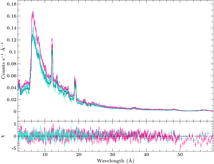
Figure 8: The LETGS spectra with the best-fitting model, consisting of a two-temperature APEC with increased neon abundance, blurred by an accretion disk. ObsID 16636 is lower-flux and plotted in turquoise, ObsIDs 15765 and 16637 are brighter and plotted in pink. For clarity, we have rebinned the spectra and combined ObsIDs 15765 and 16637, as they are spectrally very similar. The apparent emission features at $\sim$36, $\sim$48, and $\sim$57 Å are the Ne X and O VIII lines in the higher grating orders.

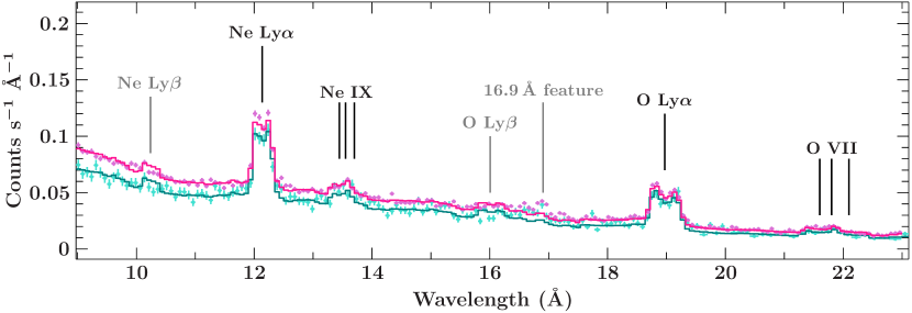
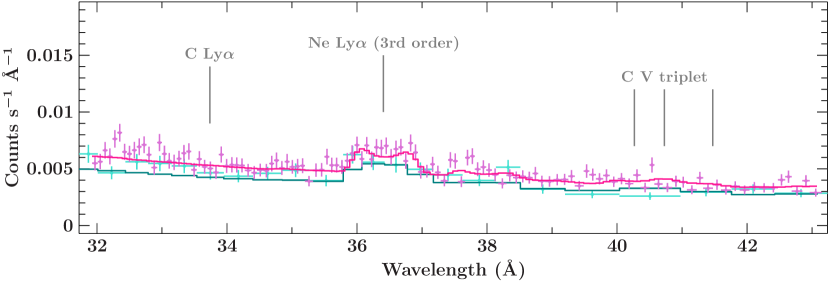
Figure 9: Emission line regions of interest, fitted with our best-fit two-temperature disk-blurred APEC model. Top: the neon and oxygen line regions. Bottom: the carbon region. Both plots show ObsID 16636 in turquoise and ObsIDs 15765 and 16637 combined in pink. Ne X Ly$\beta$ is overproduced by the model and is not detected in the spectrum. The extra emission around $16.9$ Å is of unknown origin. Carbon is not detected in emission in the X-ray spectrum, consistent with the high temperatures found by the APEC fit. The clear feature at $\sim$36.5 Å is the Ne X line in the third order; the second-order O VIII and third-order Ne IX lines are also visible in the model at $\sim$38 and 40–42 Å.

Table 5: Two-temperature disk-blurred APED fit to 4U 1626$-$67

	Parameter	Value
Plasma	Normhot ($\times 10^{-2}$ cm-5)	$4.4\pm 0.5$
	Normcool ($\times 10^{-2}$ cm-5)	$0.26\pm 0.04$
	$T_{\rm hot}$ (MK)	$13.4^{+0.7}_{-0.9}$
	$T_{\rm cool}$ (MK)	$2.30^{+0.15}_{-0.16}$
	$v_{\rm turb,hot}$ (km s-1)	$970^{+300}_{-390}$
	$v_{\rm turb,cool}$ (km s-1)	$<1210$
	C abundance	$<0.488$
	O abundance	$1$ (fixed)
	Ne abundance	$3.24^{+0.29}_{-0.28}$
	Mg abundance	$<0.190$
	Fe abundance	$0.077\pm 0.014$
Disk	$R_{\rm in}$ ($10^{3}$ $GM/c^{2}$)	$1.5^{+0.6}_{-0.4}$
	$R_{\rm out}$ ($10^{3}$ $GM/c^{2}$)	$4.3^{+3.4}_{-1.7}$
	Inclination (∘)	$34^{+8}_{-5}$
Continuum	$N_{\mathrm{H}}$ ($10^{22}$ cm-2)	$0.153\pm 0.012$
16636	$F_{0.5\text{--}10{\rm keV}}$ ($\times 10^{-10}$ erg cm-2 s-1)	$4.63$
	NormPL ($10^{-2}$ ph cm-2 s-1)	$3.4\pm 0.4$
	$\Gamma$	$1.16\pm 0.07$
	NormBB ($R_{\rm km}^{2}/D_{\rm 10}^{2}$)	$101^{+29}_{-25}$
	$kT_{\rm BB}$ (keV)	$0.499^{+0.033}_{-0.028}$
15765	$F_{0.5\text{--}10{\rm keV}}$ ($\times 10^{-10}$ erg cm-2 s-1)	$5.47$
	NormPL ($10^{-2}$ ph cm-2 s-1)	$4.0\pm 0.4$
	$\Gamma$	$1.19\pm 0.06$
	NormBB ($R_{\rm km}^{2}/D_{\rm 10}^{2}$)	$128^{+19}_{-18}$
	$kT_{\rm BB}$ (keV)	$0.520^{+0.017}_{-0.014}$
16637	$F_{0.5\text{--}10{\rm keV}}$ ($\times 10^{-10}$ erg cm-2 s-1)	$5.52$
	NormPL ($10^{-2}$ ph cm-2 s-1)	$4.1\pm 0.4$
	$\Gamma$	$1.19\pm 0.06$
	NormBB ($R_{\rm km}^{2}/D_{\rm 10}^{2}$)	$119^{+21}_{-19}$
	$kT_{\rm BB}$ (keV)	$0.519^{+0.020}_{-0.018}$
	$A_{\rm G}$ ($10^{-4}$ ph cm-2 s-1)	$8.7^{+1.4}_{-1.3}$
	$\lambda_{\rm G}$ (Å)	$16.90^{+0.06}_{-0.05}$
	$\sigma_{\rm G}$ (Å)	$0.29\pm 0.05$
	$\chi^{2}_{\nu}$ (dof)	1.11 (3883)

As with the continuum analysis, we also carried out a MCMC analysis of the rdblur-APEC model, with 100 walkers for each free parameter and a chain length of 2500. Most of the parameters are entirely consistent with the best-fit model in Table 5. The only notable difference between the MCMC results and the standard spectral fits is the carbon abundance, where the MCMC runs converge to a high abundance of $\sim$2.2, compared to the upper limit of $\sim$0.5 found in our spectral fits. This reinforces our call for caution when interpreting the carbon abundances, due to the high temperatures producing intrinsically weak carbon features.

The posterior probability distributions resulting from the MCMC runs are useful in studying correlations between the fit parameters. For instance, in Figure 10, we plot the posterior distribution for the inner disk radius and the inclination. The strong correlation is not unexpected, as the diskline and rdblur models are mostly sensitive to $R_{\rm in}\sin i$. However, the contours cut off for inclinations less than $\sim$27^∘, ruling out lower inclinations for the source. Figure 10 also shows confidence contours calculated by freezing parameters and re-fitting; these are somewhat broader than the MCMC results, but come to largely the same conclusion.

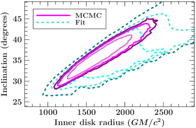
Figure 10: MCMC probability contours (magenta, solid) and traditionally-calculated confidence contours (blue, dashed) for inclination vs. inner disk radius for our rdblur-APEC model. From inside out, both show the 68%, 90%, and 95% contours. The minimum inclination allowed by the 95% contours is $\sim$25^∘, in conflict with some of the very low inclinations previously suggested for the system.

4 Discussion

4.1 The accretion disk and system inclination

The double-peaked lines of neon and oxygen are easiest to explain as originating in a disk, as other explanations typically require finely-tuned accretion geometries. For example, a bidirectional outflow could produce a two-horned line profile, but it should show a much dimmer red wing compared to the blue, as the redshifted outflow would be obscured by the accretion disk or stream. Our plasma modeling of these LETGS datasets provide excellent constraints on the disk parameters, as it fits all lines and all spectral orders simultaneously. The inner edge of the disk, if it is tracked by the emission lines, is at a radius of $\sim$1500 $GM/c^{2}$, or $3.1\times 10^{8}$ cm for a 1.4 $M_{\odot}$ neutron star. As noted above, this value is dependent on the inclination of the source, but based on Figure 10, it is unlikely to be smaller than 1000 $GM/c^{2}$. The LETGS data also provide the best limits to date on the outer radius of the emitting region, at $4300^{+3400}_{-1700}$ $GM/c^{2}$; however, it should be noted that this value is more sensitive to the choice of $q$, which we fixed in this work.

In addition to the lower limits on the line profiles and inclination shown in Figure 10, we can also note that, given the pulsar’s established spin-up trend (Camero-Arranz et al., 2010), the inner disk should lie inside of the corotation radius, which at 4U 1626$-$67’s 7.67 s pulse period is $6.5\times 10^{8}$ cm, or $\sim$3200 $GM/c^{2}$. Extrapolating from the trend in Figure 10, this implies that the inclination cannot be larger than 50–60^∘. Thus, we can conservatively conclude that, assuming the lines track the inner disk edge, the inclination likely lies in the 25–60^∘ range.

To investigate whether the emission lines really do track the inner edge of the disk, we can check that they are consistent with where we expect the inner disk to lie. The accretion disk is truncated by the neutron star’s magnetic field at the magnetospheric radius, $R_{\rm m}$, which theoretical arguments suggest should lie within the Alfvén radius, $R_{\rm A}$, given in Lamb, Pethick & Pines (1973), via Becker & Wolff (2007), as:

$$R_{\rm A}=\ 2.29\times 10^{8}\left(\frac{M_{\rm NS}}{1.4\,M_{\odot}}\right)^{-1/7}\left(\frac{R_{\rm NS}}{10{\rm\,km}}\right)^{12/7}$$

$$\times\left(\frac{B}{10^{12}{\rm\,G}}\right)^{4/7}\left(\frac{\dot{M}}{10^{17}{\rm\,g\,s^{-1}}}\right)^{-2/7}{\rm\,cm},$$ (2)

where $B$ is the magnetic field strength of the star (here assumed to be dipolar), $\dot{M}$ is the accretion rate, and $M_{\rm NS}$ and $R_{\rm NS}$ are the mass and radius of the neutron star. Assuming an accretion rate of $1.1\times 10^{16}$ g s^-1 as found by Schulz, Chakrabarty & Marshall (2019), a dipole magnetic field strength of $4.2\times 10^{12}$ G, based on the CRSF energy measured by D’Aì et al. (2017), and a canonical 1.4 $M_{\odot}$, 10 km radius neutron star, $R_{\rm A}$ is approximately $10^{9}$ cm, or $\sim$4800 $GM/c^{2}$. Our inner disk radius of $\sim$1500 $GM/c^{2}$ is thus $\sim$0.3$R_{\rm A}$, in line with theoretical predictions and similar to estimates of $R_{\rm m}/R_{\rm A}$ for other sources (e.g., Filippova et al., 2017).

4.2 Plasma modeling

4.2.1 Chemical abundances in 4U 1626$-$67

Our APEC fits give us a useful handle on the chemical abundances in the system. However, the abundances reported in Table 5 are relative to the solar abundances of Anders & Grevesse (1989), while the donor star is hydrogen-depleted. Thus, we measure the elemental abundances relative to oxygen by fixing the oxygen abundance to unity. Following Schulz, Chakrabarty & Marshall (2019), it is straightforward to determine the number density ratio between some chosen element X and oxygen:

$$\frac{n_{\rm X}}{n_{\rm O}}=\frac{\rm Abund(X)}{\rm Abund(O)}\left(\frac{n_{\rm X}}{n_{\rm H}}\right)_{\rm AG89}\left(\frac{n_{\rm O}}{n_{\rm H}}\right)_{\rm AG89}^{-1},$$ (3)

where $n_{\rm X}$ is the number density of element X, Abund(X) is the abundance for the same element returned by APEC, and $\left(n_{\rm X}/n_{\rm H}\right)_{\rm AG89}$ is taken from the Anders & Grevesse (1989) abundance tables.

From the upper limits and measurements found in Table 5, we find $n_{\rm Ne}/n_{\rm O}=0.47\pm 0.04$, $n_{\rm Mg}/n_{\rm O}\lesssim 0.0085$, and $n_{\rm Fe}/n_{\rm O}=0.0042\pm 0.0008$. For carbon, we find $n_{\rm C}/n_{\rm O}\lesssim 0.21$ from our spectral fits and $n_{\rm C}/n_{\rm O}\sim 0.93$ from our MCMC results. However, as noted earlier, this discrepancy probably arises from the non-detection of any carbon features at all. More quantitatively, Figure 11 displays the fraction of ions in the H-like and He-like states as a function of temperature, as calculated by AtomDB. At our best-fit temperatures (the shaded regions in Figure 11), carbon is mostly in the fully-ionized state, producing intrinsically weak carbon features. In contrast, magnesium should be mostly in the H- and He-like states, so the lack of Mg lines, under the collisional plasma assumption, is better explained by an intrinsically low abundance. We do not plot ionization fractions for iron, but as noted in Section 3.4, at these temperatures iron is mostly in the Fe XVII and Fe XXIII states — a range of ions with plenty of X-ray lines in the LETGS’ band.

Specifically on the iron abundance, Koliopanos & Gilfanov (2016) carried out an extensive study of 4U 1626$-$67’s Fe K$\alpha$ fluorescence line, finding an inner disk radius from the line width of 3.7–$15.7\times 10^{8}$ cm (1800–7600 $GM/c^{2}$) — somewhat larger but not inconsistent with our measurements. However, they also derived a considerably lower iron abundance, quoting an O/Fe ratio approximately 68 times the solar value, while our measurement implies a ratio between 10 and 15 times solar. There are likely significant systematic effects that both analyses ignore — our measurement stems from the lines hiding in the wings of the Ne X feature and upper limits on lines in the 15 Å region in what is assumed to be a fully collisionally-ionized, optically thin plasma (in reality, the optically thin assumption may not hold and photoionization likely plays a not insignificant role, viz. the lack of a Ne X K$\beta$ and the 17 Å feature discussed in Section 4.2.2), while Koliopanos & Gilfanov (2016) assume a C/O-dominated plasma, a lamppost geometry, and a Shakura & Sunyaev (1973) disk (the disk is likely hotter hotter and heated by X-ray heating from the pulsar, clearly contains significant neon, and may contain helium, per the discussion in Schulz, Chakrabarty & Marshall, 2019).

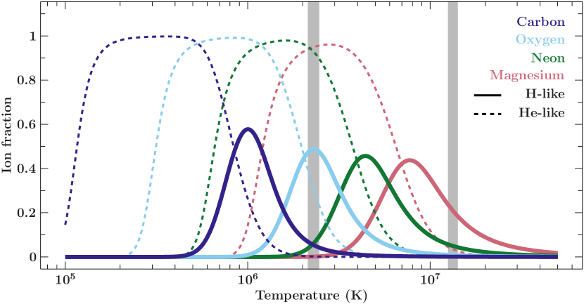
Figure 11: The ionization fractions of H-like and He-like carbon, oxygen, neon, and magnesium for a range of temperatures. The hydrogen-like ions are plotted with solid lines, and the helium-like ions are plotted with dashed lines. Our measured temperatures of $13$ and $2.3$ MK are indicated by the gray shaded regions. Carbon is almost fully ionized at 2 MK and completely ionized at 13 MK, explaining its lack of presence in the X-ray spectrum. Magnesium, on the other hand, should have a significant fraction in the Mg XII state, meaning the lack of emission from magnesium is better explained by a lack of magnesium in the system.

4.2.2 The 16.9 Å feature and collisional vs. photoionization

While our disk-blurred collisional plasma model fits these datasets quite well, it fails in two main areas: first, the Ne X K$\beta$ feature is overpredicted by the APEC plasma model, and second, there is additional emission around 16.9Å that is consistently unmodeled. Furthermore, as found by Schulz, Chakrabarty & Marshall (2019) and in Section 3.3, the two temperature components of the APEC plasma appear to originate around the same radial distance, suggesting some sort of complex geometry (e.g., a clumpy environment or an azimuthal temperature distribution) or that the two-temperature model is only an approximation for a more complex system. These give us some insight into the true nature of the plasma.

The Ne X K$\beta$ line

For this undermodeled feature at 10.24 Å, the discrepancy between model and data may lie in the APEC model’s assumption of an optically-thin plasma. The Ne X K$\beta$ photons are more sensitive to optical depth — in a more optically thick plasma, they can be scattered into Ly$\alpha$ and UV photons, while Ly$\alpha$ photons have no alternative transitions. Thus, careful simulations of a plasma with a higher optical depth may obtain a better fit in this area.

The 16.9 Å feature

The excess emission at 16.9 Å is somewhat more perplexing. It appears in all three datasets and in both the positive and negative orders, and does not appear to be a second- or third-order artifact (as there does not appear to be excess emission at 8.45 or 5.63 Å). Considering the instrument calibration, the LETGS’ effective area curve does have the two M edges of cesium to either side of this feature, but the excess flux is quite high for a calibration feature. Fitted with a Gaussian, the equivalent width of the feature is 12 eV in the first observation and 10 eV in the last two, and the velocity width is $\sim$5200 km s^-1. However, it is also acceptably well-fit by a diskline profile centered slightly red- or blueward of the peak. The feature seen in the LETGS is too dim to be detected in the HETGS observations investigated in Schulz, Chakrabarty & Marshall (2019).

There are no strong emission lines around 17 A that would not be accompanied by brighter lines at other wavelengths (e.g., Fe XVII should also show emission at 15 and 16 A). Variations on our collisional plasma model (e.g., adding a third temperature component and/or more aggressive variation of elemental abundances) fail to reproduce the extra emission. However, the radiative recombination continuum (RRC) of oxygen does lie around 16–17 A. Our APEC-based model does not produce strong RRCs due to the high temperature, but we find that adding a photemis component with $\log\xi\sim 1$ and the same abundances as our APEC plasma produces a clear oxygen RRC which, when blurred by the disk, recovers some of the excess emission around 16.9 Å (while avoiding the strong neon RRC that appeared in the pure photemis fits of Schulz, Chakrabarty & Marshall, 2019). The comparison between our pure APEC model and an APEC+photemis model is shown in Figure 12. It should be noted that this is somewhat of an ad-hoc approach to the problem and we do not claim that the photemis component reflects the actual physical reality of the system — not only does photemis assume a far lower density ($10^{4}$ cm^-3) and temperature (4800 K) than we see in 4U 1626$-$67, but the normalization of $\sim$100 required to produce the model displayed in Figure 12 implies an emitting region several orders of magnitude larger than the entire 4U 1626$-$67 system. Nonetheless, this should provide something of a starting point for more self-consistent modeling of this source, and at least demonstrates that an oxygen RRC, when blurred by the disk, can reproduce the shape of the observed feature at 16.9 Å. It is also interesting to note that our ionization parameter, $\log\xi\sim 1$, is similar to the ionization parameter predicted in Schulz, Chakrabarty & Marshall (2019).

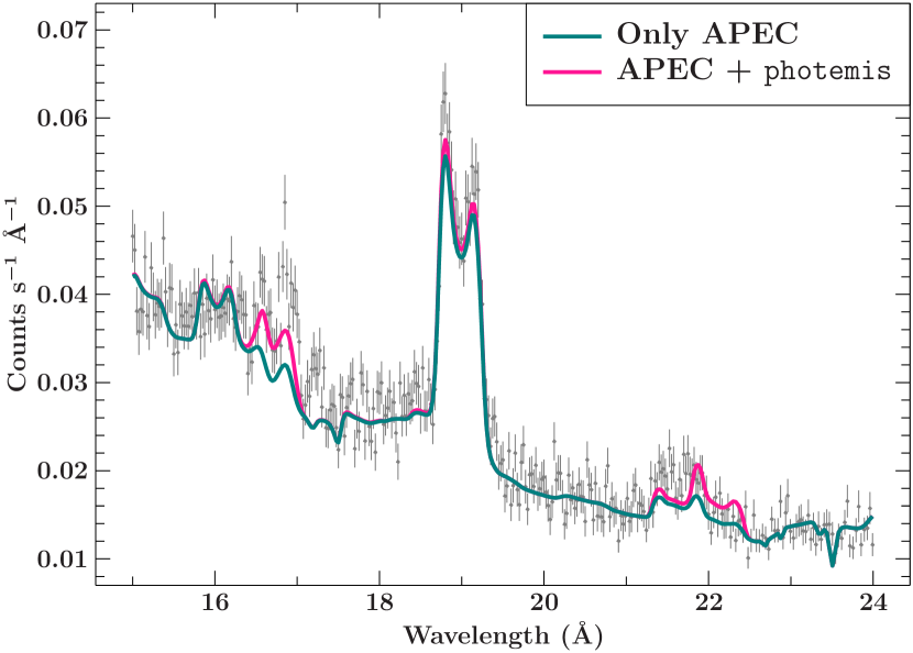
Figure 12: The oxygen region of the LETGS spectrum, comparing our two-temperature APEC model with and without an additional photemis component. The oxygen RRC, when blurred by the disk, begins to reproduce the excess emission at 16.9 Å

4.3 On the nature of the donor star

In Figure 13, we plot the relationship between inclination and donor mass, assuming a 1.4 $M_{\odot}$ neutron star, based on the observed lack of eclipses in the source and the published limit of $a\sin i<8$ lt-ms from Shinoda et al. (1990). We assume a circular, 42-minute orbit and that the donor fills its Roche lobe, the radius of which we take from Eggleton (1983). The relationship between inclination and orbit size is from Chakrabarty (1998). Our measurement of $i\gtrsim 27^{\circ}$ thus implies a donor mass $M_{\rm d}\lesssim 0.026$ $M_{\odot}$; higher inclinations would require progressively lower-mass donors. This is independent of the precise nature of the donor — as long as the donor fills its Roche lobe and the disk inclination reflects the orbit inclination, these constraints must be met. The question, then, is what type of companion can reach this low of a mass, fill its Roche lobe, produce the chemical abundances we observe, and provide a high enough accretion rate to explain the spin-up and X-ray flux?

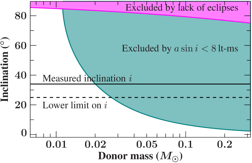
Figure 13: Limits on the inclination and donor mass in 4U 1626$-$67. The upper magenta shaded region indicates the upper limit on the inclination from the lack of eclipses in the system, based on the Roche lobe radius for the donor at that mass. The large teal shaded region is excluded due to the measured limit on the semimajor axis of $a\sin i<8$ lt-ms. Our measured inclination is indicated by a solid black line, and the approximate lower limit on the inclination from our confidence contours and MCMC runs is indicated by a dashed black line.

UCXBs, outside of globular clusters, are generally believed to follow one of three possible formation channels, based on three different classes of donor stars: hydrogen-depleted main-sequence stars, helium-burning stars, and white dwarfs. As noted by Nelemans et al. (2010), the donor in any UCXB is almost certainly some sort of degenerate, low-mass dwarf, as in the main-sequence and helium-burning cases, the degenerate core of the star will be exposed by mass transfer. Thus, the differences between these donors will be mainly observable in their chemical composition and mass.

Verbunt, Wijers & Burm (1990) and Chakrabarty (1998) rejected the helium-burning donor case, as this would either be orders of magnitude brighter in the optical or orders of magnitude dimmer in the X-rays. For the evolved main-sequence donor, while 4U 1626$-$67’s low hydrogen fraction does present a problem for this case, Nelemans et al. (2010) state that such donors could have hydrogen fractions as low as $\sim$10^-5, and while the hydrogen fraction in 4U 1626$-$67 is certainly low ($\lesssim$0.1, per Werner et al., 2006), it is not clear that it is low enough to fully rule this case out. However, per Verbunt, Wijers & Burm (1990), the mass-radius relationship for such an object means it would need to have a mass of about 0.08 $M_{\odot}$ to fill its Roche lobe at 4U 1626$-$67’s orbital period, which is quite strongly ruled out by our limits on the inclination.

Thus, we are left with a white dwarf (that is, some kind of compact stellar remnant supported primarily by electron degeneracy pressure) as the donor. As noted by Deloye & Bildsten (2003), the possible types of white dwarf donors exist more on a continuum than as a discrete set of classes, defined mainly by the mass of the original main-sequence star and its age at the onset of mass transfer — a system that began mass transfer while the donor was burning helium will have a different composition compared to one that began after a white dwarf had formed.

Previous work has favored C/O or O/Ne compositions for the donor, based on the bright neon and oxygen lines and the lack of detected helium. However, both C/O and O/Ne white dwarfs present issues from the composition standpoint. Taking the C/O case, with equal parts carbon and oxygen, the neon fraction in 4U 1626$-$67 must be $\sim$0.2–0.3 based on our spectral fits. This is in fairly strong disagreement with models of C/O white dwarfs, which typically predict neon fractions of at most a few percent. Even if one considers chemical fractionation (e.g., Segretain et al., 1994), the neon fraction is a factor of a few too large. On the O/Ne side, the neon fraction is no longer an issue, but we find the opposite problem with magnesium — the magnesium fraction in an O/Ne white dwarf should be of order 10%, while we constrain it to below a percent. Furthermore, in Schulz, Chakrabarty & Marshall (2019), we argued that helium must be present in order to keep the emitting volume within reasonable limits, given the plasma emission measure we obtain; however, this must be brought into agreement with the lack of detected helium in the visible and UV (Homer et al., 2002; Werner et al., 2006) — but it should also be noted that Werner et al. (2006)’s work failed to detect neon in the visible spectrum, in conflict with our clearly detected neon features. The work presented here and in Schulz, Chakrabarty & Marshall (2019) provide very strong limits on the mass of the donor star, the geometry of the accretion disk, and the chemical abundances in the system, but considerably more sophisticated plasma and accretion disk modeling is needed to properly interpret these results.

5 Conclusion

Our detailed analysis of the LETGS dataset on 4U 1626$-$67 converges on a picture of an accretion disk which is inclined at $\sim$34^∘ (somewhat high relative to previous estimates) and dominated by collisional ionization (although with some contribution from photoionization), with a large overabundance of neon relative to oxygen and underabundances of magnesium and iron. Our measurements of the inner edge of the accretion disk constrain it to a lower limit of $\sim$1000 $GM/c^{2}$, or $2\times 10^{8}$ cm, which is approximately 20% of the neutron star’s Alfvén radius and well within its corotation radius. Based on the emission line profiles and 4U 1626$-$67’s spin-up trend, the inclination is constrained to between 25 and 60^∘. The donor star must be very low-mass, $\lesssim$0.026 $M_{\odot}$, in order to meet the constraints on the size of the system, and its chemical composition and plasma characteristics suggest it is a helium white dwarf. In the following, we summarize some of the remaining issues with this system and attempt to suggest some ways forward.

5.1 Mass transfer rate

Evolutionary scenarios for UCXBs generally find systems reaching a minimum period of $\sim$10 minutes relatively quickly, followed by a longer-timescale migration outwards towards longer orbital periods. Many of these scenarios (e.g., those of Yungelson, Nelemans & van den Heuvel, 2002; Nelemans et al., 2010) predict mass-transfer via gravitational radiation in the $10^{-12}$–$10^{-11}$ $M_{\odot}$  yr^-1 range, typically 1–2 orders of magnitude too low given 4U 1626$-$67’s X-ray flux. With the 3.5 kpc distance found by Schulz, Chakrabarty & Marshall (2019), this discrepancy is ameliorated somewhat, but not entirely — the source is still approximately an order of magnitude brighter than mass transfer via gravitational radiation would predict.

There are some possible mechanisms for driving more mass transfer. Heinke et al. (2013) argued that 4U 1626$-$67 had to be a persistent accretor, rather than a long-duration transient, based on estimating the total accreted mass and arguing that this was larger than the maximum mass of a helium or carbon-oxygen disk. The source’s continued X-ray emission to this day means these arguments are still valid even considering the shorter distance from Schulz, Chakrabarty & Marshall (2019). Heinke et al. presented models starting from helium-burning stars which fit 4U 1626$-$67’s accretion rate and orbital period, although more work would need to be done to make sure that such a donor does not burn too much helium, as this would conflict with the plasma emission measure arguments in Schulz, Chakrabarty & Marshall (2019). Their suggested donor’s mass on reaching a 42 min orbit may also be slightly high compared to our limits presented here, although they only consider a few possible models and there may be room in the parameter space in this regard. Another solution might be found in the irradiation of the donor — Lü et al. (2017) find that X-ray irradiation of very low-mass white dwarf donors in UCXBs can drive long-duration outbursts, lasting as long as centuries for $\sim$0.01 $M_{\odot}$ donors. These suggest very different natures for 4U 1626$-$67: under the model presented by Heinke et al. (2013), 4U 1626$-$67 is a truly persistent source; under Lü et al. (2017)’s argument, it is a very long-duration transient.

5.2 Accretion disk composition and donor star

Under the assumption of a two-temperature, collisionally-ionized plasma, we find a Ne/O ratio that is $3.24^{+0.29}_{-0.28}$ times solar, corresponding to a value of $0.47\pm 0.04$. This model largely reproduces the observed spectrum with the exception of an overproduced Ne X Ly$\beta$ line and a line-like feature at 16.9 Å, which we argue in Section 4.2.2 likely stems from an unmodeled photoionized component of the spectrum. In reality, as argued in Schulz, Chakrabarty & Marshall (2019), the disk of 4U 1626$-$67 likely sits in an intermediate state where the assumptions of common plasma models such as APEC and photemis fail to fully describe the system. In particular, the very high density suggested in Schulz, Chakrabarty & Marshall (2019) approaches or exceeds the limit where APEC and XSTAR models are valid.

Our large Ne/O ratio and small Mg/O ratio are difficult to reconcile with most He-depleted white dwarf models — we find too much neon for a C/O white dwarf, which will have a neon fraction of only a few percent, while a O/Ne white dwarf should have a magnesium fraction of 5–10% (see, e.g., Dominguez, Tornambe & Isern, 1993; García-Berro, Ritossa & Iben, 1997; Gil-Pons & García-Berro, 2001), far in excess of the magnesium abundance we find. This is consistent with our findings in Schulz, Chakrabarty & Marshall (2019), where we argued based on the plasma emission measure that very little helium burning could have taken place in 4U 1626$-$67, thus concluding that the donor is likely a helium white dwarf. This, however, must be reconciled with the lack of helium features in the optical spectra — Werner et al. (2006) placed a limit on the helium fraction of $\lesssim$10%. Of course, Werner et al. (2006) also found little evidence for neon in the system, while in the X-rays the presence of neon is incontrovertible, so there are clearly significant discrepancies between the optical and X-rays. The specific physics of the disk are an obvious place to look here — for example, the Shakura & Sunyaev (1973) disk used as a baseline by Werner et al. (2006)’s model, at their assumed accretion rate, has a total luminosity of a few $\times 10^{33}$ erg s^-1. The APEC component in our best-fit model, in comparison, has a luminosity of $\sim 5\times 10^{34}$ erg s^-1 — an order of magnitude higher. Helium and neon could thus be in a higher ionization state than considered by Werner et al. (2006) — although this, in turn, would need to be reconciled with the fact that Werner et al. do see oxygen features, which would be unexpected if temperatures were high enough to ionize neon to the point of non-detection.

5.3 Accretion disk parameters and inclination

The strong double-peaked emission lines in the LETGS spectrum provide some of the best constraints to date on the parameters of the accretion disk, and are largely consistent with those found using the HETGS (Schulz, Chakrabarty & Marshall, 2019). While the inner disk radius and inclination are obviously degenerate with each other (Figure 10), we still obtain good lower limits on the inner disk radius ($\sim$1000 $GM/c^{2}$) and inclination ($\sim$27^∘). On the high-inclination end, the neutron star’s spin-up trend means the inner disk cannot be farther out than the corotation radius, $\sim$3200 $GM/c^{2}$, which, extrapolating from Figure 10, limits the inclination to $\lesssim 60^{\circ}$.

These bounds, with a best-fit value of ${34^{\circ}}^{+8}_{-5}$, indicate a somewhat high inclination compared to other estimates. Most recently, in Iwakiri et al. (2019), we carried out a full general relativistic raytracing analysis of the hard X-ray pulse profiles of 4U 1626$-$67, which converged on an inclination of $9.5^{\circ}\pm 0.2$. However, as stated in Iwakiri et al. (2019), the large number of free parameters and systematic factors in such an analysis means the model presented is not unique, and there is at least one other solution at an inclination of 27^∘ (albeit with considerably more complex beam patterns). Thus, we think while this disagreement is interesting, it is not necessarily something to be particularly concerned about at this moment.

However, it is of interest to note that the inclinations measured here and in Iwakiri et al. (2019) have slightly different definitions: our measurement is of the inclination of the inner edge of the accretion disk, assuming Keplerian rotation, while Iwakiri et al.’s is the inclination of the spin axis of the neutron star. If the spin axis and accretion disk were misaligned, this would produce a systematic difference between the two measurements. Such a scenario would likely drive a warp in the inner disk, which would precess at some rate and could explain 4U 1626$-$67’s torque reversals and quasi-periodic flaring (see Figure 1). This is not a new idea — Wijers & Pringle (1999) suggested that a warp in the inner disk could have flipped through 90^∘ to produce 4U 1626$-$67’s 1990 torque reversal, and Chakrabarty et al. (2001) interpreted a 1 mHz QPO in the optical as arising from a precessing warp in the disk. Precession of the disk would produce variation in the inclination measured by the emission lines; the fact that we do not observe any significant changes in the line profiles between these LETGS observations taken within a few days of each other tells us that if precession is occurring, it is probably not on a timescale of days. Shorter timescales are likely too short for Chandra to probe effectively; however, future missions with high spectral resolution and larger effective area (e.g., Lynx) may be able to investigate this.

5.4 Accretion-induced collapse

4U 1626$-$67 is fundamentally an odd system, with an apparently-young neutron star (long pulse period, strong magnetic field) in orbit with an apparently-old donor. The rough timescale for UCXB formation is $\sim 10^{9}$ yr (van Haaften et al., 2012), while magnetic field decay is estimated to be a $10^{8}$ yr process (e.g., Bhattacharya et al., 1992), although this depends strongly on the initial conditions and mechanisms considered. One solution that has been proposed to reconcile these is that the neutron star formed via accretion-induced collapse, which could sidestep some timescale-related issues. Yungelson, Nelemans & van den Heuvel (2002) theorized that a 1.2 $M_{\odot}$ ONeMg white dwarf could undergo AIC and produce a 1.26 $M_{\odot}$ neutron star in a 4U 1626$-$67-like system after about 350 Myr. This is an attractive scenario at first glace: with a large amount of accretion in this system falling onto the original white dwarf and not the neutron star, magnetic burial could be avoided, and the additional time could possibly allow for crystallization to produce the enhanced neon abundance we observe.

However, there are at least two serious issues with the AIC scenario. First, an AIC event would produce a $\sim$160 Myr gap before accretion resumed onto the neutron star, during which the neutron star would cool. This could actually enhance the decay of the magnetic field due to ambipolar diffusion: per Goldreich & Reisenegger (1992), the timescale for this process is $\sim 3$ Gyr at a core temperature of $10^{8}$ K, but this drops below 100 Myr at a temperature of a few $10^{6}$ K. Building on this in a recent paper, Cruces, Reisenegger & Tauris (2019) found that a neutron star with an initial core temperature of $3\times 10^{8}$ K and a $10^{12}$ G field could drop to $\sim 10^{8}$ G in less than 100 Myr. Thus, it is not at all clear that a post-AIC binary would still retain a highly-magnetized neutron star once accretion resumes. Additionally, it may be difficult to evolve an AIC event into a 4U 1626$-$67-like system with a short orbital period and very low-mass companion — Tauris et al. (2013)’s study of accretion-induced collapse found that for close-orbit, post-AIC systems, the donors retain masses between 0.65 and 0.85 $M_{\odot}$, considerably larger than 4U 1626$-$67’s 0.02 $M_{\odot}$ donor.

A detailed study of this subject is obviously beyond the scope of this paper, but our results here may provide some useful context and constraints for future studies.

References

- Anders & Grevesse (1989) Anders, E., & Grevesse, N., 1989, Geochimica et Cosmochimica Acta, 53, 197
- Angelini et al. (1995) Angelini, L., White, N. E., Nagase, F., Kallman, T. R., Yoshida, A., Takeshima, T., Becker, C., & Paerels, F., 1995, The Astrophysical Journal, 449, L41
- Becker & Wolff (2007) Becker, P. A., & Wolff, M. T., 2007, The Astrophysical Journal, 654, 435
- Beri, Paul & Dewangan (2015) Beri, A., Paul, B., & Dewangan, G. C., 2015, Monthly Notices of the Royal Astronomical Society, 451, 508
- Bhattacharya et al. (1992) Bhattacharya, D., Wijers, R. a. M. J., Hartman, J. W., & Verbunt, F., 1992, Astronomy and Astrophysics, 254, 198
- Brinkman et al. (2000) Brinkman, B. C., et al., 2000, X-Ray Optics, Instruments, and Missions III, 4012, 81
- Camero-Arranz et al. (2010) Camero-Arranz, A., Finger, M. H., Ikhsanov, N. R., Wilson-Hodge, C. A., & Beklen, E., 2010, The Astrophysical Journal, 708, 1500
- Camero-Arranz et al. (2012) Camero-Arranz, A., Pottschmidt, K., Finger, M. H., Ikhsanov, N. R., Wilson-Hodge, C. A., & Marcu, D. M., 2012, Astronomy and Astrophysics, 546, A40
- Chakrabarty (1998) Chakrabarty, D., 1998, The Astrophysical Journal, 492, 342
- Chakrabarty et al. (1997) Chakrabarty, D., et al., 1997, The Astrophysical Journal, 474, 414
- Chakrabarty et al. (2001) Chakrabarty, D., Homer, L., Charles, P. A., & O’Donoghue, D., 2001, The Astrophysical Journal, 562, 985
- Cruces, Reisenegger & Tauris (2019) Cruces, M., Reisenegger, A., & Tauris, T. M., 2019, arXiv e-prints, arXiv:1906.06076
- D’Aì et al. (2017) D’Aì, A., Cusumano, G., Del Santo, M., La Parola, V., & Segreto, A., 2017, Monthly Notices of the Royal Astronomical Society, 470, 2457
- Deloye & Bildsten (2003) Deloye, C. J., & Bildsten, L., 2003, The Astrophysical Journal, 598, 1217
- Dominguez, Tornambe & Isern (1993) Dominguez, I., Tornambe, A., & Isern, J., 1993, The Astrophysical Journal, 419, 268
- Eggleton (1983) Eggleton, P. P., 1983, The Astrophysical Journal, 268, 368
- Erickson (1977) Erickson, G. W., 1977, Journal of Physical and Chemical Reference Data, 6, 831
- Fabian et al. (1989) Fabian, A. C., Rees, M. J., Stella, L., & White, N. E., 1989, Monthly Notices of the Royal Astronomical Society, 238, 729
- Filippova et al. (2017) Filippova, E. V., Mereminskiy, I. A., Lutovinov, A. A., Molkov, S. V., & Tsygankov, S. S., 2017, Astronomy Letters, 43, 706
- Finger et al. (2009) Finger, M. H., et al., 2009, in 2009 Fermi Symposium, ed. W. N. Johnson, D. J. Thompson, eConf proceedings C0911022)
- Foreman-Mackey et al. (2013) Foreman-Mackey, D., Hogg, D. W., Lang, D., & Goodman, J., 2013, Publications of the Astronomical Society of the Pacific, 125, 306
- Foster et al. (2012) Foster, A. R., Ji, L., Smith, R. K., & Brickhouse, N. S., 2012, ApJ, 756, 128
- Fruscione et al. (2006) Fruscione, A., et al., 2006, in Society of Photo-Optical Instrumentation Engineers (SPIE) Conference Series, ed. D. R. Silva, R. E. Doxsey, Vol. 6270, 62701V
- García-Berro, Ritossa & Iben (1997) García-Berro, E., Ritossa, C., & Iben, I., 1997, The Astrophysical Journal, 485, 765
- Giacconi et al. (1972) Giacconi, R., Murray, S., Gursky, H., Kellogg, E., Schreier, E., & Tananbaum, H., 1972, The Astrophysical Journal, 178, 281
- Gil-Pons & García-Berro (2001) Gil-Pons, P., & García-Berro, E., 2001, Astronomy and Astrophysics, 375, 87
- Goldreich & Reisenegger (1992) Goldreich, P., & Reisenegger, A., 1992, The Astrophysical Journal, 395, 250
- Heinke et al. (2013) Heinke, C. O., Ivanova, N., Engel, M. C., Pavlovskii, K., Sivakoff, G. R., Cartwright, T. F., & Gladstone, J. C., 2013, The Astrophysical Journal, 768, 184
- Homer et al. (2002) Homer, L., Anderson, S. F., Wachter, S., & Margon, B., 2002, The Astronomical Journal, 124, 3348
- Houck & Denicola (2000) Houck, J. C., & Denicola, L. A., 2000, in Astronomical Data Analysis Software and Systems IX, ed. N. Manset, C. Veillet, D. Crabtree, Vol. 216, 591
- Huenemoerder et al. (2011) Huenemoerder, D. P., et al., 2011, The Astronomical Journal, 141, 129
- Ilovaisky, Motch & Chevalier (1978) Ilovaisky, S. A., Motch, C., & Chevalier, C., 1978, Astronomy and Astrophysics, 70, L19
- Iwakiri et al. (2019) Iwakiri, W. B., et al., 2019, The Astrophysical Journal, 878, 121
- Joss, Avni & Rappaport (1978) Joss, P. C., Avni, Y., & Rappaport, S., 1978, The Astrophysical Journal, 221, 645
- Koliopanos & Gilfanov (2016) Koliopanos, F., & Gilfanov, M., 2016, Monthly Notices of the Royal Astronomical Society, 456, 3535
- Krauss et al. (2007) Krauss, M. I., Schulz, N. S., Chakrabarty, D., Juett, A. M., & Cottam, J., 2007, The Astrophysical Journal, 660, 605
- Lamb, Pethick & Pines (1973) Lamb, F. K., Pethick, C. J., & Pines, D., 1973, The Astrophysical Journal, 184, 271
- Leahy et al. (1983) Leahy, D. A., Darbro, W., Elsner, R. F., Weisskopf, M. C., Kahn, S., Sutherland, P. G., & Grindlay, J. E., 1983, The Astrophysical Journal, 266, 160
- Lü et al. (2017) Lü, G., Zhu, C., Wang, Z., & Iminniyaz, H., 2017, The Astrophysical Journal, 847, 62
- McClintock et al. (1977) McClintock, J. E., Bradt, H. V., Doxsey, R. E., Jernigan, J. G., Canizares, C. R., & Hiltner, W. A., 1977, Nature, 270, 320
- Middleditch et al. (1981) Middleditch, J., Mason, K. O., Nelson, J. E., & White, N. E., 1981, The Astrophysical Journal, 244, 1001
- Nelemans, Jonker & Steeghs (2006) Nelemans, G., Jonker, P. G., & Steeghs, D., 2006, Monthly Notices of the Royal Astronomical Society, 370, 255
- Nelemans et al. (2010) Nelemans, G., Yungelson, L. R., Sluys, V. D., V, M., & Tout, C. A., 2010, Monthly Notices of the Royal Astronomical Society, 401, 1347
- Orlandini et al. (1998) Orlandini, M., et al., 1998, The Astrophysical Journal, 500, L163
- Pottschmidt et al. (2018) Pottschmidt, K., et al., 2018, American Astronomical Society Meeting Abstracts
- Rappaport et al. (1977) Rappaport, S., Markert, T., Li, F. K., Clark, G. W., Jernigan, J. G., & McClintock, J. E., 1977, The Astrophysical Journal, 217, L29
- Schulz, Chakrabarty & Marshall (2019) Schulz, N. S., Chakrabarty, D., & Marshall, H. L., 2019, submitted to ApJ, arxiv:1911.11684
- Schulz et al. (2001) Schulz, N. S., Chakrabarty, D., Marshall, H. L., Canizares, C. R., Lee, J. C., & Houck, J., 2001, The Astrophysical Journal, 563, 941
- Segretain et al. (1994) Segretain, L., Chabrier, G., Hernanz, M., Garcia-Berro, E., Isern, J., & Mochkovitch, R., 1994, The Astrophysical Journal, 434, 641
- Shakura & Sunyaev (1973) Shakura, N. I., & Sunyaev, R. A., 1973, Astronomy and Astrophysics, 24
- Shinoda et al. (1990) Shinoda, K., Kii, T., Mitsuda, K., Nagase, F., Tanaka, Y., Makishima, K., & Shibazaki, N., 1990, Publications of the Astronomical Society of Japan, 42, L27
- Tauris et al. (2013) Tauris, T. M., Sanyal, D., Yoon, S.-C., & Langer, N., 2013, Astronomy and Astrophysics, 558, A39
- van Haaften et al. (2012) van Haaften, L. M., Nelemans, G., Voss, R., Wood, M. A., & Kuijpers, J., 2012, Astronomy and Astrophysics, 537, A104