Geodesic structure and quasinormal modes of a tidally perturbed spacetime

Abstract

Tidal perturbations play an important role in the study of the dynamics in the classical two-body system. Understanding tidal effects in strong-field regions may allow one to use gravitational-wave or electromagnetic observations to locate or constraint the location of possible companions. Here, we investigate how timelike and null geodesics of a Schwarzschild black hole are affected in the presence of a companion. There is a panoply of new effects. In some limiting cases, we find analytical solutions for closed null or timelike geodesics. Our results show that light ring period as measured by a far-away observer can be eiter shorter or longer, depending on the location of the companion. We also show that there are closed lightlike trajectories which are elliptic (for equatorial companions), and that timelike particles are affected in a similar manner. Finally, we attempt at estimating the ringdown from tidally perturbed geometries. Our results indicate that there are two stages in the relaxation of such geometries, one associated with a prompt decay of waves around the deformed photonsphere, and a later relaxation of the global geometry. These results are consistent with previous, full numerical studies.

I Introduction

Tidal interactions play a fundamental role in many astrophysical systems. The best known example are the oceans tides in the Earth-Moon system, which drive tidal acceleration and longer days, but their effects are ubiquitous in astrophysics. In the context of gravitational-wave (GW) astronomy, of tests of fundamental physics and of strong-field gravity, tidal effects are precious. In a compact binary emitting GWs, tidal deformations induced by the companion affect the GW phase. The amount of the de-phasing (relative to that of pointlike objects) correlates to the equation of state of the inspiralling bodies, hence a precise monitoring of the GW phase evolution can teach us about the equation of state of neutron star binaries (Flanagan and Hinderer, 2008; Dietrich et al., 2020; Gupta et al., 2020). Black holes (BHs) have a particularly simple equation of state, owing to the uniqueness properties in vacuum General Relativity Chrusciel et al. (2012); Cardoso and Gualtieri (2016). Hence, the tidal interactions of compact objects are particularly useful to test the Kerr nature of BHs Cardoso et al. (2017); Sennett et al. (2017); Cardoso and Pani (2019, 2019).

Previous studies explored the potential of tidal interactions to constrain the presence of a possible massive companion to the Sgr*A source Naoz et al. (2020). Specifically, data collected by the GRAVITY collaboration Abuter et al. (2018, 2020) on the orbital motion of the star S0-2 was used to constrain possible orbital parameters of such a companion. It was also shown that a putative companion may give rise to GW emission potentially detectable with the future space-based interferometer LISA. The effect of tidal fields in Newtonian orbits is, of course, well studied, specially in the restricted three-body problem (see Refs. Murray and Dermott (2000); Domingos et al. (2008) and references therein). Here, we want to understand the effects of weak tides in the strong-field region. We are particularly interested on the effect of tides on the location and properties of the innermost stable circular orbit (ISCO), and of the photonsphere. These dictate the high-energy behavior of accretion disks, and the relaxation properties of BHs Chandrasekhar (1983); Cardoso et al. (2009, 2016); Yang (2021), and so can be useful smoking-guns of companions. Driven by similar motivations, this problem was studied recently, albeit in less realistic setups. The position of the ISCO was studied in a spacetime describing a binary of extremal charged BHs, in particular the Majumdar-Papapetrou dihole spacetime Nakashi and Igata (2019a, b). The photonsphere of binary BH spacetimes has been the subject of recent studies Assumpcao et al. (2018); Bernard et al. (2019); Daza et al. (2018), since it may help in understanding the relaxation or ringdown stage of binaries themselves, or hold the key to understanding how the individual components quasinormal ringdown is affected by the companion. These spacetimes include, naturally, tidal effects, but their effects have mostly been studied numerically. Our aim is to provide simple analytical results of strong field phenomena. We use geometric units $G=c=1$ throughout.

II Setup: a black hole perturbed by a companion

Consider a non-spinning BH of mass $M$, perturbed by a companion of mass $M_{c}$ at a distance $R$. For far-away companions, the tide is weak and one can expand the geometry around its Schwarzschild value,

$$g_{\mu\nu}=g_{\mu\nu}^{\rm Sch}+\epsilon\,h_{\mu\nu}\,,$$ (1)

where $\epsilon$ represents the strength of the tidal perturbation, assumed to be small ($\epsilon\ll 1$). Using Regge and Wheeler’s approach, the perturbation $h_{\mu\nu}$ can be expanded in tensor spherical harmonics Regge and Wheeler (1957); Zerilli (1970); Berti et al. (2009) and decomposed in polar and axial parts, due to the spherical symmetry of the system. We focus on the polar contributions which, in the Regge-Wheeler gauge, can be written as:

$$h_{\mu\nu}^{\rm polar}=\left(\begin{matrix}fH_{0}^{lm}&H_{1}^{lm}\,&0&0\\ H_{1}^{lm}&f^{-1}H_{2}^{lm}&0&0\\ 0&0&r^{2}K^{lm}&0\\ 0&0&0&r^{2}\sin^{2}\theta K^{lm}\end{matrix}\right)Y^{lm}\,\,$$ (2)

where $H_{i}^{lm}=H_{i}^{lm}(t,r)$, $K^{lm}=K^{lm}(t,r)$, $Y^{lm}=Y^{lm}(\theta,\phi)$ are standard spin-0 spherical harmonics and

$$f=f(r)=\left(1-\frac{2M}{r}\right)\,.$$ (3)

To continue, consider a companion far away, such that the orbital timescale is larger than any other scale in the problem and much larger than the timescale of the internal dynamics of the body. In this regime, one can focus on static perturbations. The vacuum field equations then provide equations for the metric functions $H_{0},H_{1},H_{2},K$. These should be solved demanding regularity at the horizon. We will mostly focus on quadrupolar modes, but the analysis is easily extended. The $tr$ and $\theta\theta$ components of the field equations result in

$$H_{1}=0\,,\qquad H_{2}=H_{0}\,.$$ (4)

The solution for $H_{2}$ which is regular across the horizon $r=2M$ for $l=2$ is given by

$$H_{2}=\,c_{1}\frac{3\,(2M-r)\,r}{M^{2}}=-\frac{3\,c_{1}}{M^{2}}\,r^{2}\,f(r)\,,$$ (5)

where $c_{1}$ is an integration constant that must be determined by studying the asymptotic behaviour of the metric (1) in the presence of an external tidal field. This can be done using the definition of multipole moments developed by Thorne Thorne (1980); Zhang (1986). The effects of an external tidal field are entirely encoded in two symmetric and trace-free tensors: the polar tidal field $\mathcal{E}_{L}$ and the axial tidal field $\mathcal{B}_{L}$. The polar tidal field can be expanded in spherical harmonics as $\mathcal{E}_{L}x^{L}=r^{l}\sum_{m}\mathcal{E}_{lm}Y^{lm}(\theta_{c},\phi_{c})$, where $\theta=\theta_{c}$ and $\phi=\phi_{c}$ are the angular coordinates of the companion in the BH sky Binnington and Poisson (2009).

In the most general case, the asymptotic expansion of the metric will depend on the angular index $m$. Since we only need it to find the value of $c_{1}$, we can fix $m=0$ without loss of generality and the metric expansion reads

$$\begin{split}g_{tt}&=-1+\frac{2M}{r}+\sum_{l\geq 2}\left[\frac{2}{r^{l+1}}\left(\sqrt{\frac{4\pi}{2l+1}}M_{l}Y^{l0}+(l^{\prime}<l\,\text{pole})\right)\right.\\ &-\left.\frac{2}{l(l-1)}r^{l}[\mathcal{E}_{l}Y^{l0}+(l^{\prime}<l\,\text{pole})]\right]\,,\end{split}$$ (6)

where $M_{l}$ are the mass multipole moments.

If we consider the dominant quadrupolar contribution with $l=2$, we can match Eq. (6) with the $tt$-component of Eq. (1), and find

$$c_{1}=\frac{M^{2}\,\mathcal{E}_{2}}{3}\,.$$ (7)

Now we have to find the explicit value of the tidal moment $\mathcal{E}_{2}$. This can be done matching the full metric  (1) with a Post Newtonian (PN) description of the external spacetime Binnington and Poisson (2009); Poisson and Will (1953). We will always assume parameters for which the system can be captured by a PN description. The $g_{tt}$ component in the PN approximation is Poisson and Will (1953):

$$g_{tt}^{\rm PN}=-1+2U(r,\theta,\phi)\,.$$ (8)

If we assume that the companion is a PN monopole of mass $M_{c}$ and centering ouselves in the BH frame, the potential can be written as

$$U = \frac{M}{r}+\frac{M_{c}}{|\mathbf{r}-\mathbf{R}|}$$ (9)

$$= \frac{M}{r}+M_{c}\sum_{lm}\frac{4\pi}{2l+1}\frac{r^{l}}{R^{l+1}}Y^{*}_{lm}(\theta_{c},\phi_{c})Y_{lm}(\theta,\phi).$$

Finally for $l=2$ we have

$$g_{tt}^{\rm PN}=-1+\frac{2M}{r}+\frac{8\pi M_{c}}{5}\frac{r^{2}}{R^{3}}\,\sum_{m}Y^{*}_{2m}(\theta_{c},\phi_{c})\,Y_{2m}(\theta,\phi)\,,$$ (10)

and comparing (10) with the $g_{tt}$ component of the perturbed metric we find that

$$\mathcal{E}_{2}=-\frac{8\pi M_{c}}{5R^{3}}\sum_{m}\,Y^{*}_{2m}(\theta_{c},\phi_{c})=-\frac{8\pi\epsilon}{5M^{2}}\,\sum_{m}Y^{*}_{2m}(\theta_{c},\phi_{c})\,,$$ (11)

where in the last step we have defined the strength of the tidal deformation as

$$\epsilon=M^{2}M_{c}/R^{3}\,.$$ (12)

Equation (11) agrees with the expression for $\mathcal{E}_{2}$ in Cardoso et al. (2020). The metric functions in (2) are now completely determined and they read:

$$H_{0}(r) = H_{2}(r)=\frac{8\pi\epsilon}{5M^{2}}\,r^{2}f(r)\sum_{m}Y^{*}_{2m}(\theta_{c},\phi_{c})\,,$$ (13)

$$K(r) = \frac{8\pi\epsilon}{5M^{2}}\left(r^{2}-2M^{2}\right)\sum_{m}Y^{*}_{2m}(\theta_{c},\phi_{c})\,.$$ (14)

III Polar companions

We will specialize our calculations to two specific setups, where the orbits lie in the BH-companion plane, or orthogonal to it. Equivalently, and this is the approach we follow, we restrict to equatorial orbits, and place the companion either at the equator or at the pole.

We start with a companion at the pole, $\theta_{c}=0,\,\phi_{c}=0$, which then preserves the azimuthal symmetry of the BH.

III.1 ISCO and light ring properties

The full components of the metric with $l=2$ on the equatorial plane are:

$$g_{tt}^{\rm polar} = -f(r)\left[1+f(r)\,\frac{r^{2}\,\epsilon}{M^{2}}\right]\,,$$ (15)

$$g_{rr}^{\rm polar} = g(r)-\frac{r^{2}\,\epsilon}{M^{2}}\,,$$ (16)

$$g_{\theta\theta}^{\rm polar} = g_{\phi\phi}^{\rm polar}=r^{2}\left[1-\frac{(r^{2}-2M^{2})}{M^{2}}\,\epsilon\right]\,.$$ (17)

In the equatorial plane, we then find the Lagrangian

$$2\mathcal{L}=g_{tt}^{\rm polar}\dot{t}^{2}+g_{rr}^{\rm polar}\dot{r}^{2}+g_{\phi\phi}^{\rm polar}\dot{\phi}^{2}\,,$$ (18)

with dots standing for derivatives with respect to proper time. The Lagrangian is time and azimuth independent, giving rise to two conserved quantities, specific energy $E$ and angular momentum $L$

$$\dot{t} = \frac{E}{f(r)(1+\epsilon fr^{2}/M^{2})}\,,$$ (19)

$$\dot{\phi} = \frac{L}{r^{2}(1+(2-r^{2}/M^{2})\,\epsilon)}\,.$$ (20)

The equations of motion are easier to handle via an effective radial potential, which can be obtained substituting (19)-(20) in the normalization for the quadrivelocity

$$g_{\mu\nu}\,u^{\mu}u^{\nu}=\delta\,,$$ (21)

where $\delta=0,-1$ for null and timelike geodesics, respectively. One finds,

$$\dot{r}^{2}=E^{2}-V_{\delta}(r)\,,$$ (22)

where

$$V_{\delta}(r) = \frac{L^{2}\,(2M-r)\left(2Mr\epsilon-2r^{2}\epsilon+M^{2}(2\epsilon-1)\right)}{M^{2}r^{3}}$$ (23)

$$+ \delta\frac{(2M-r)\,(M^{2}-2Mr\epsilon+r^{2}\epsilon)}{M^{2}r}\,.$$

To understand the ISCO properties, we expand all relevant quantities in Eq. (23) to first order in $\epsilon$, e.g., $r_{\rm ISCO}=r^{(0)}+\epsilon\,r^{(1)}$, with $r^{(0)}=6M$ the unperturbed Schwarzschild BH value. By definition, at the ISCO $E^{2}-V_{(\delta=-1)}=dV_{(\delta=-1)}/dr=d^{2}V_{(\delta=-1)}/dr^{2}=0$. We find

$$r_{\rm ISCO} = 6M(1-256\epsilon)\,,$$ (24)

$$E_{\rm ISCO} = \frac{2\sqrt{2}}{3}\left(1+38\epsilon\right)\,,$$ (25)

$$L_{\rm ISCO} = 2\sqrt{3}M(1+7\epsilon)\,,$$ (26)

$$\Omega_{\rm ISCO} = \frac{1+491\epsilon}{6\sqrt{6}\,M}\,.$$ (27)

Note that $\Omega_{\rm ISCO}$ is simply $\dot{\phi}/\dot{t}$ evaluated at the ISCO, and is the angular velocity as measured by far away observers.

Table 1: Numerical results for the ISCO properties of a tidally deformed BH spacetime. The analytical results (24)-(27) agree with these values up to the last digit.

	Numerical results
$\epsilon$	$r/M$	$E$	$L/M$
$10^{-7}$	5.9998	0.94281	3.4641
$10^{-6}$	5.9985	0.94284	3.4644
$10^{-5}$	5.9849	0.94317	3.4671
$10^{-4}$	5.8657	0.94633	3.4932

High frequency photons or gravitons are well described by null geodesics. Of these, there is one that stands out: a close null geodesic which for non-rotating, isolated BHs is located at $r=3M$ Chandrasekhar (1983); Cardoso et al. (2009, 2016); Cardoso and Pani (2019); Yang (2021). This location defines the light ring or photosphere. In the presence of a companion, we find

$$r_{\rm LR} = 3M(1+5\epsilon)\,,$$ (28)

$$b_{\rm LR} = 3\sqrt{3}M(1-5\epsilon)M\,,$$ (29)

$$\Omega_{\rm LR} = \frac{1+5\,\epsilon}{3\sqrt{3}\,M}\,.$$ (30)

where $b=L/E$ is the impact parameter.

These analytical estimates can be compared to a numerical solution of the geodesic equations. Those results are shown in Table 1 for some selected values of $\epsilon$. The perturbative analytical results agree with these numbers to all digits listed. These results can be compared and contrasted to those referring to an extremally-charged BH binary, the Majumdar-Papapetrou geometry. This is done in Appendix .1.

III.2 The relaxation of tidally perturbed black holes: light ring modes and quasinormal modes

Consider now fundamental fields in the BH vicinities, such as gravitational or electromagnetic waves. The dynamical evolution is described by a set of second order differential equations whose details depend on the initial data. In general however, the time evolution is characterized by a prompt signal, followed by a ringdown which is caused by the “leaky” boundary conditions at the boundaries Leaver (1986); Berti et al. (2009). When new structure is added, such as a change of boundary conditions at large distances or in the near-horizon region, new features appear. In particular, the light ring controls the early-time relaxation of BHs, whereas the late-time ringdown is dictated by boundary conditions, defining quasinormal modes Cardoso et al. (2009); Yang et al. (2012); Cardoso et al. (2016); Cardoso and Pani (2017, 2019). For isolated BHs, these two decays coincide and the dynamical properties of BHs are relatively simple.

We are dealing with a tidally perturbed BH, so we expect two stages in the dynamical evolution of fundamental massless fields. In fact, there is evidence in the literature for such distinctive behavior Bernard et al. (2019). Consider, first, the light ring relaxation. A complete knowledge must be obtained performing time evolutions of the corresponding evolution equations, but a good description is obtained in the eikonal approximation Cardoso et al. (2009); Yang et al. (2012). In this approximation, the early time ringdown of a signal $\Phi$ is an exponentially damped sinusoid,

$$\Phi\sim e^{-\omega_{I}^{\rm LR}t}\sin{\omega_{R}^{\rm LR}t}\,.$$ (31)

Formally, the signal is a superposition of overtones which carry an associated index $\ell$ associated with the angular dependence and an index $n$ associated to a radial dependence. Here, the ringdown frequency $\omega_{R}^{\rm LR}$ and the damping rate $\omega_{I}^{\rm LR}$ are given by the angular frequency (30) and the Lyapunov exponent $\lambda=\sqrt{V_{r}^{{}^{\prime\prime}}/2\,\dot{t}^{2}}$, respectively Cardoso et al. (2009).

Although this limit is formally valid only when $\ell\gg 1$, it has been shown that it gives very accurate results even when $\ell$ is smaller Berti et al. (2009). In particular for modes with $\ell=m$ we have $\omega_{R}=\ell\,\Omega_{\rm LR}$ and $\omega_{I}=(n+1/2)|\lambda_{\rm LR}|$. For $\ell=m=2$ the ringdown frequency and the damping rate are

$$M\omega_{R}=\frac{2\,(1+5\,\epsilon)}{3\sqrt{3}}\,,\quad M\omega_{I}=\left(n+\frac{1}{2}\right)\frac{1-10\,\epsilon}{3\,\sqrt{3}}\,.$$ (32)

We thus have a clear prediction for the changes in the early ringdown of GWs, induced by a companion.

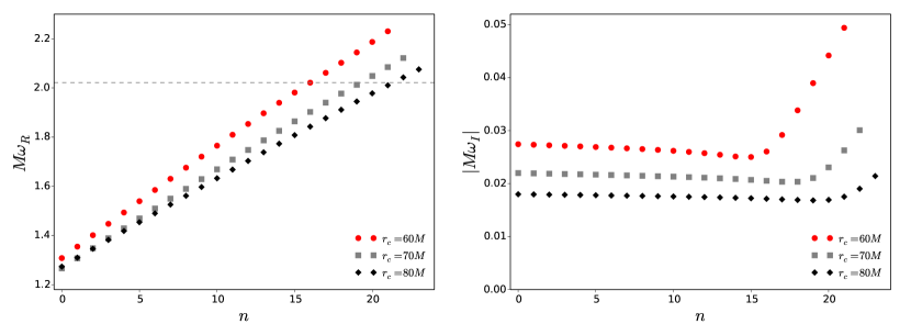
Figure 1: Real (left panel) and imaginary (right panel) part of the frequencies for different values of the “cutoff point” $r_{c}$ in the function $H(r)$. In this case $\epsilon=10^{-4}$, $k=100$, and $l=m=10$. The dashed line represents the Schwarzschild frequency (not shown in the right panel since its value $|M\omega_{I}|^{\rm Sch}\simeq 0.09$ is out of the range chosen).

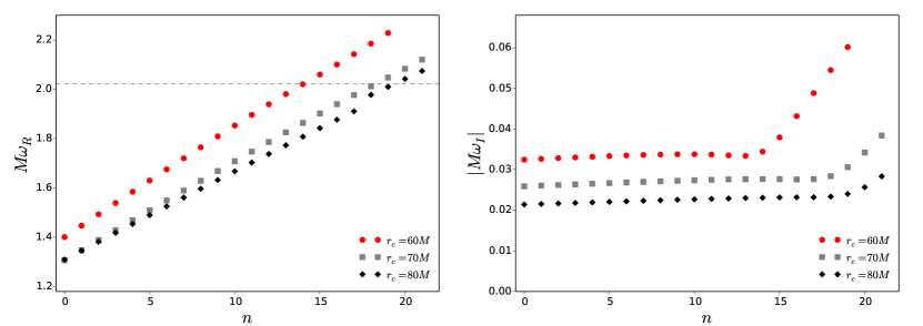
Figure 2: Real (left panel) and imaginary (right panel) part of the frequencies for different values of the “cutoff point” $r_{c}$ in the function $H(r)$. In this case $\epsilon=10^{-4}$, $k=2$ and $l=m=10$. The dashed line represents the Schwarzschild frequency (not shown in the right panel since its value $|M\omega_{I}|^{\rm Sch}\simeq 0.09$ is out of the range chosen).

Now, as we mentioned, the late time behavior of the GW signal is dominated by the poles of the relevant Green function the quasinormal modes (QNMs), and therefore are sensitive to the entire geometry and not only to the local properties around the light ring. In order to assess the QNM spectrum one needs to solve the dynamics. To understand the possible changes, we focus on the relatively simpler problem of a scalar field propagating on the fixed, background geometry (1). The dynamics are governed by the Klein-Gordon equation,

$$\Box\varphi=\frac{1}{\sqrt{-g}}\partial_{\mu}\left(g^{\mu\nu}_{\rm polar}\sqrt{-g}\,\partial_{\nu}\varphi\right)=0\,,$$ (33)

where $g=\det{g^{\rm polar}_{\mu\nu}}$. Since the spacetime admits two Killing vectors $\partial_{t}$ and $\partial_{\phi}$, we can decompose the scalar field as:

$$\varphi(t,r,\theta,\phi)=e^{i(m\phi-\omega t)}\frac{\psi_{l}(r)}{r}Y_{lm}(\theta)\,.$$ (34)

If we substitute Eq. (34) in Eq. (33) we get a system of differential equations that are not separable. Following Ref. Cano et al. (2020), we can expand the box operator in (33) at first order in $\epsilon$:

$$\Box=\Box_{(0)}+\epsilon\,\Box_{(1)}\,,$$ (35)

where we have taken into account that the zeroth order part is separable while the non-separable terms come only from the perturbative correction to the metric. The explicit form of the operator is

$$\Box_{(0)}\varphi_{m,\omega}(r,\theta)=\frac{1}{r^{2}}\partial_{r}\left(r(r-2M)\partial_{r}\varphi\right)$$ (36)

$$+ \frac{1}{r^{2}\sin\theta}\partial_{\theta}\left(\sin\theta\,\partial_{\theta}\varphi\right)+\left[\frac{r\,\omega^{2}}{r-2M}-\frac{m^{2}}{r^{2}\sin^{2}\theta}\right]\varphi\,,$$

$$\frac{2M^{2}}{1+3\cos 2\theta}\Box_{(1)}\varphi_{m,\omega}(r,\theta)=\frac{2M^{2}-r^{2}}{r^{2}}\cot\theta\partial_{\theta}\varphi$$ (37)

$$+ \frac{2M^{2}-r^{2}}{r^{2}}\partial_{\theta}^{2}\varphi-\frac{2(r-2M)^{2}}{r}\partial_{r}\varphi-(r-2M)^{2}\partial_{r}^{2}\varphi$$

$$+ \left(r^{2}\omega^{2}+\frac{(r^{2}-2M^{2})}{r^{2}\sin^{2}\theta}m^{2}\right)\varphi\,.$$

Since the zeroth-order solution for a given $l_{0}$ is $\varphi(r,\theta)=\psi_{l_{0}}(r)/r\,Y_{l_{0}m}(\theta)$, it is possible and consistent to assume that any term with $l\neq l_{0}$ comes from the perturbative correction. Hence, we can expand the solution such as,

$$\varphi_{m,\omega}(r,\theta)=\frac{\psi_{l_{0}}(r)}{r}Y_{l_{0}m}(\theta)+\epsilon\sum_{l\neq l_{0}}\frac{\psi_{l}(r)}{r}Y_{lm}(\theta)$$ (38)

Applying the operator (35) to the solution (38) and negleting terms $\mathcal{O}(\epsilon^{2})$ we have:

$$\Box_{(0)}\left[\frac{\psi_{l_{0}}(r)}{r}Y_{l_{0}m}(\theta)\right]+\epsilon\sum_{l\neq l_{0}}\Box_{(0)}\left[Y_{lm}(\theta)\frac{\psi_{l}(r)}{r}\right]+$$

$$+\epsilon\,\Box_{(1)}\left[\frac{\psi_{l_{0}}(r)}{r}Y_{l_{0}m}(\theta)\right]+\mathcal{O}(\epsilon^{2})=0\,.$$ (39)

Projecting (39) onto $Y_{l_{0}m}(\theta)$ we get one single radial equation that can be solved numerically to find the QNM frequencies:

$$\left(\Box_{(0)}-l(l+1)\right)\frac{\psi_{l_{0}}(r)}{r}$$ (40)

$$+ \epsilon\int_{0}^{\pi}\Box_{(1)}\left[\frac{\psi_{l_{0}}(r)}{r}Y_{l_{0}m}(\theta)\right]Y_{l_{0}m}(\theta)d\theta=0\,.$$

The asymptotic behavior of the solutions of the above equation are as follows,

$$\psi_{l_{0}} \sim (r-2M)^{2Mi\omega}\,,\qquad r\to 2M\,,$$ (41)

$$\psi_{l_{0}} \sim \,e^{\pm\omega r}\,,\qquad r\to\infty\,.$$ (42)

The boundary condition at the horizon is similar to that of isolated BHs Berti et al. (2009). However, the boundary behavior at large spatial distances, imposed on us by the equations of motion, are completely different from those of an asymptotically flat spacetime. Indeed, the metric perturbation of the tidally perturbed BH we’re studying is not asymptotically flat. We are using the diverging piece of the metric perturbation to impose the presence of a companion far away. In a complete setup, the companion is at finite distance and the spacetime asymptotically flat. In other words, our description of the binary system is only accurate for distances $r\lesssim R$. The boundary conditions imposed on us within this setup are similar to those of asymptotically anti-de Sitter or other spacetimes where radiation is confined Berti et al. (2009); Brito et al. (2014). They select a set of complex quasinormal mode frequencies

$$\omega=\omega_{R}+i\omega_{I}\,.$$ (43)

Accordingly, the confining nature of the tidal perturbations indicates that one will find a QNM spectrum which differs substantially from that of a single Schwarzschild BH, reflecting the fact that perturbations should be less damped (as the only dissipation channel is now the horizon).

We thus need to fix the unacceptable behavior at large spatial distances. We will do so without entering the challenge of matched asymptotic expansions to correctly reproduce the geometry everywhere Bernard et al. (2019). We simply “cutoff” the tidal effects with an auxiliary function, which we take rather arbitrarily to have the form $H(r)=1/1+e^{2k(r-r_{c})}$. In other words, our regularization procedure consists on the replacement

$$\epsilon\rightarrow\frac{\epsilon}{1+e^{2k(r-r_{c})}}\,,$$ (44)

since the $\epsilon$ terms are precisely the ones responsible for the divergence at infinity. In general, results will depend on the smoothness parameter $k$ and the cutoff point $r_{c}$. It seems reasonable to ask that $r_{c}\sim R$, whereas $k$ is at least of the order $M_{c}$ to describe a smooth transition.

Figures 1-2 show the QNMs for three different values of the cutoff radius $r_{c}/M=60,\,70,\,80$ and $k=100$ (top panels) or $k=2$ (bottom panels). Notice that what is shown are the first overtones. Since we are mostly interested in comparing against the eikonal limit, we fix $\ell=m=10$. We fixed a tidal parameter $\epsilon=10^{-4}$, but results for other $\epsilon$ are similar.

As already anticipated from the discussion above, the most salient feature of Figs. 1-2 is that the QNM spectrum of a tidally deformed BH is completely different from that of an isolated BH. Despite our curing the asymptotic behavior artificially, remains of this behavior remain in the perturbation via the existence of quasi-bound states. For example, for a perturbation parameter $\epsilon=10^{-4}$, one could expect a correspondingly small change in the QNM spectrum. However, as can be seen in Figs. 1-2, the QNM frequencies change by ${\cal O}(1)$. These features were seen in the past Leung et al. (1997); Barausse et al. (2014); Brito et al. (2014); Cardoso et al. (2016); Cardoso and Pani (2019) and are connected with the asymptotic properties of the effective potential for wave propagation (and of the corresponding solutions). In fact, the tidal effects act to create a long-distance “well” that traps low frequency radiation. This explains why the damping of the lowest modes (see right panels in Figs. 1-2) is so much lower than the isolated-BH counterpart. Once the vibration frequency $\omega_{R}$ is sufficiently large for fluctuations to tunnel out through the light ring, $\omega_{R}\simeq\omega_{R}^{\rm Sch}$ Cardoso et al. (2009), a new channel for dissipation is open, and the damping timescale decreases.

Our results are well described by a real component

$$\omega_{R}\approx\omega_{R}^{(0)}+\alpha\,n\,,\quad n=0,1,2...$$ (45)

where the offset $\omega_{R}^{(0)}$ corresponds to the fundamental mode $n=0$, and $\alpha$ is a constant, which decreases increasing $r_{c}$ and it is independent (or only weakly dependent) on $\epsilon$. Our results indicate a very weak dependence of $\omega_{R}^{(0)}$ on $r_{c}$ and $\epsilon$. At very small $\epsilon$ we recover the Schwarzschild fundamental QNM, but it is not necessarily the fundamental mode of this perturbed spacetime. This is the spectrum characteristic of a confined system and differs markedly from that of an isolated BH, for which the (real part of the) QNM frequencies asymptote to a constant Berti et al. (2009). For $k=100$, $\alpha=0.044,\,0.039,\,0.035$ for $r_{c}/M=60,\,70,\,80$ respectively, while for $k=2$, $\alpha=0.052,0.048,0.041$.

Regarding the imaginary part of the QNM frequencies, our results for the fundamental mode are well described by

$$M\omega_{I}^{(0)}\approx\frac{3M}{5\,r_{c}\,\epsilon^{1/8}}\,.$$ (46)

As we stressed, these results are sensitive to the cutoff function and radius we choose. We have also investigated the auxiliary function $H(r)=\Theta(r_{c}-r)$, with $\Theta$ the Heaviside function. Our results for the QNM spectrum show the same qualitative behavior as in Figs. 1-2. Although the numerical values are slightly different, the overall structure is the same, and we find frequencies below the Schwarzschild fundamental mode. We also find a transition in the spectrum at $\omega_{R}\simeq\omega_{R}^{\rm Sch}$, as before. This lends strength to the claim that Figs. 1-2 are a good qualitative description of the spectrum.

In conclusion, there are two different stages to consider in the relaxation of binaries Bernard et al. (2019). The first one is associated with a prompt ringdown phase and the local properties of the BHs light ring, which are affected by the presence of the companion via (32). This is a local property of the spacetime and hence is not affected by the asymptotic structure at infinity. The second one is associated with the late time decay of the field which instead strongly depends on the global properties of the spacetime and that we tried to capture solving (40). Although it is impossible with our naive cutoff procedure to fully capture all the physics, the structure of the spectrum confirms that we’re dealing with a very different late-time relaxation induced by the different scales in the problem. These features have already been seen in the numerical studies of Ref. Bernard et al. (2019).

IV Equatorial companions

We now specialize our analysis to equatorial companions, for which $\theta_{c}=\pi/2$. Without loss of generality we can impose $\phi_{c}=0$. The presence of the companion, which is still assumed to be at rest, breaks the axisymmetry of the metric. As a consequence, the orbits that now lie on the BH-companion plane, have an explicit dependence on the azimuthal angle. For $\ell=2$, the metric components read:

$$g_{tt}^{\rm eq} = \frac{f(r)}{2M^{2}}\left[-2M^{2}+f(r)\,r^{2}\epsilon\left(1+3\cos 2\phi\right)\right]\,,$$ (47)

$$g_{rr}^{\rm eq} = \frac{g(r)}{2M^{2}}\left[2M^{2}-2Mr\epsilon+r^{2}\epsilon+3r(r-2M)\epsilon\cos 2\phi\right]\,,$$ (48)

$$g_{\theta\theta}^{\rm eq} = g_{\phi\phi}^{\rm eq}$$ (49)

$$= \frac{r^{2}}{2M^{2}}\left[2M^{2}(1-\epsilon)+r^{2}\epsilon+3(r^{2}-2M^{2})\epsilon\cos 2\phi\right]\,.$$

IV.1 Null geodesics

Table 2: Coordinate value of $r_{0}$ at $\theta=\pi/2,\,\phi=0$ for which the null geodesic is closed. We show both the numerical result $r_{0}^{\rm num}$ and the analytical prediction $r_{0}^{\rm an}$ given in Eq. (54) and valid for small $\epsilon$.

$\epsilon$	$3-r_{0}^{\rm num}/M$	$3-r_{0}^{\rm an}/M$
$10^{-6}$	$1.2\times 10^{-5}$	$1.2\times 10^{-5}$
$10^{-5}$	$1.2\times 10^{-4}$	$1.2\times 10^{-4}$
$10^{-4}$	$1.2\times 10^{-3}$	$1.2\times 10^{-3}$
$10^{-3}$	$1.2\times 10^{-2}$	$1.2\times 10^{-2}$

Due to the non-axisymmetry of the spacetime, solving geodesic motion analytically is challenging. Instead, we perform a numerical integration of geodesic equations and find the best fit for the motion’s parameters. Consider first null geodesics and the “shape” of closed null orbits. To calculate these, we integrate the geodesic equations subjected to initial conditions,

$$x_{0}^{\alpha}=\left(0,r_{0},\pi/2,0\right)\,,\quad u_{0}^{\alpha}=\left(u_{0}^{\phi}/s,0,0,u_{0}^{\phi}\right)\,,$$ (50)

where $s=\sqrt{-g_{tt}(r_{0},\pi/2,0)/g_{\phi\phi}(r_{0},\pi/2,0)}$. These conditions ensure that we’re integrating the motion for a null particle. We then vary the affine parameter $\tau$ in an interval $\left[0,\Upsilon\right]$ and fine-tune the value $r_{0}\sim 3M$ such that the orbit closes in the same interval. The period (in proper or affine time) $\Upsilon$ is roughly given by $\sim 2\pi/u_{0}^{\phi}$ and hence our calculation is independent from the initial value of $u^{\phi}$.

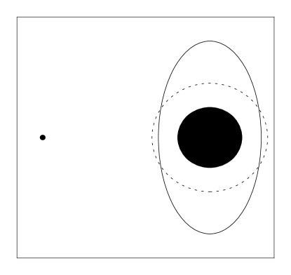
Figure 3: Graphic representation of the closed null orbit (54) (solid line) when the companion is fixed at the equator. The dashed circle represents the light ring in the Schwarzschild spacetime. Not in scale.

Our results show an interesting, perhaps expected feature (cf. Fig. 3): the null geodesic is no longer circular, but there are closed null orbits, which are elliptical. In fact, one can describe them analytically at small $\epsilon$, looking for an expansion with the functional form

$$r(\phi) = 3M-\epsilon(x_{0}+A\cos 2\phi(\tau))M\,,$$ (51)

$$\phi(\tau) = (c_{1}+\epsilon c_{2})\frac{\tau}{M}\,,$$ (52)

$$t(\tau) = t_{0}\tau+\epsilon(t_{1}+B\sin 2\phi(\tau))M\,.$$ (53)

The geodesic equations, together with the normalization for quadri-velocities, yield the solution

$$r(\phi) = 3M-\epsilon\left(\frac{15}{2}+\frac{9}{2}\cos 2\phi(\tau)\right)M\,,$$ (54)

$$t(\tau) = t_{0}\tau+\frac{45\sqrt{3}}{4}\epsilon\sin 2\phi(\tau)M\,,$$ (55)

$$\phi(\tau) = t_{0}\left(\frac{1}{3\sqrt{3}}-\frac{5}{6\sqrt{3}}\epsilon\right)\frac{\tau}{M}\,,$$ (56)

where $t_{0}$ is a scale-factor of the affine parameter $\tau$ (with no influence on observables). Table 2 reports the values of $r_{0}$ (at $\phi=0$) obtained via numerical integration and the analytical prediction (54). Once the solution (54) is known, one can find the parameters of the ellipse in terms of $\epsilon$. Namely, $a=(3-3\epsilon)M$ and $b=(3-12\epsilon)M$ are the semi-major and semi-minor axes respectively, while the eccentricity is given by $e=\sqrt{\frac{6\epsilon}{1-4\epsilon}}$.

Imposing $\phi(\Upsilon)=2\pi$, one can find the period of the orbit, which in the $t$-coordinate is

$$T=t(\Upsilon)=3\sqrt{3}\pi(2+5\epsilon)\,M\,.$$ (57)

IV.2 Timelike geodesics: particles at rest

Table 3: Location $r_{s}$ where static equilibrium of particles in a tidally deformed BH spacetime is possible. Numerical values are denoted $r_{s}^{\rm num}$ and can be compared against the analytical prediction $r_{s}^{\rm an}$ of Eq. (59).

$\epsilon$	$r_{s}^{\rm num}/M$	$r_{s}^{an}/M$
$10^{-6}$	80.037	79.713
$10^{-5}$	37.507	37.195
$10^{-4}$	17.766	17.479
$10^{-3}$	8.604	8.372

The spacetime described by Eqs.  (47)-(49) seems to admit new types of motion. We find new results concerning static particles, i.e., orbits which satisfy $\dot{r}=\dot{\phi}=0$. At $\tau=0$, we set initial conditions $\phi=0,\,r=r_{s}$ and the radial motion is governed by

$$\dot{r}^{2}=E^{2}+(2M-r_{s})\left(\frac{1}{r_{s}}-\frac{2(r_{s}-2M)\epsilon}{M^{2}}\right)\,.$$ (58)

Solving $\dot{r}=\ddot{r}=0$, one finds:

$$r_{s} = \left(\frac{2}{3}+\frac{1}{(2\epsilon)^{1/3}}\right)M+\mathcal{O(\epsilon)}\,,$$ (59)

$$E^{2} = 1+\mathcal{O(\epsilon)}\,.$$ (60)

Estimates (59) can be tested solving numerically the geodesic equations imposing $u_{0}^{t}=\sqrt{-1/g_{tt}^{\rm eq}(r_{s},\pi/2,0)}$ as initial condition. Table 3 reports the results obtained with these two approaches, with an overall good agreement.

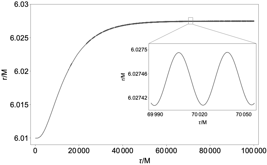
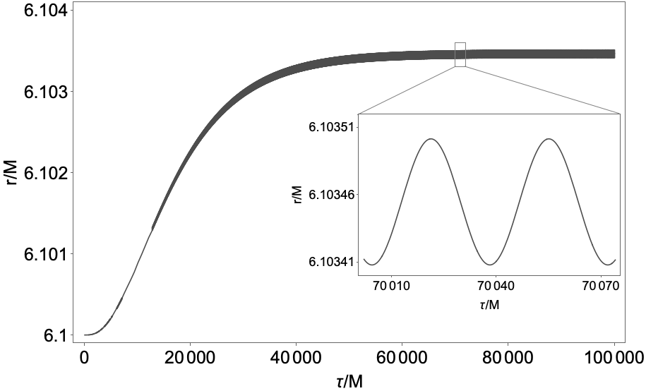
Figure 4: Orbital radius of a particle, as function of proper time $\tau$. The particle is placed initially on a circular trajectory of radius $r_{i}=6.01M$ (left panel) and $r_{i}=6.10M$ (right panel) and perturbed by a companion such that $R(\tau)=R_{0}/(1-e^{-\lambda(\tau+\delta)})$, with $\lambda=10^{-4}$, $\delta=10^{-4}$, $R_{0}=200M$. The inset shows the behaviour of the radial coordinate on shorter timescales for $r_{i}/M=6.01,6.10$. Oscillations with periodicity $\sim 45M$ can be seen, which correspond to orbital periods $\sim 90M$ in the $(r,\phi)$-plane, in accordance with Fig. (5) and Table 4. Note that at early times there are some “gaps” in the oscillatory behaviour. These are a technical artifact of plot-drawing only and have no physical meaning.

The result (59) is also in agreement with a Newtonian solution of the problem (Butikov, 2002; Hjorth and Knudsen, 1996). Consider a binary system with masses $M$ and $M_{c}$ separated by a distance $R$. Let a test particle with mass $\mu$ be located at distance $r$ from the primary mass $M$. The test particle will be at rest if the gravitational force exerted by the primary mass is compensated by the tidal force exerted by the secondary mass on the primary. Namely,

$$\frac{M\mu}{r^{2}} = \frac{M_{c}\mu}{(R-r)^{2}}-\frac{M_{c}\mu}{R^{2}}\simeq\frac{2M_{c}\mu r}{R^{3}}\,,$$ (61)

where we have exploited the fact that $r/R\ll 1$. Solving this equation for $r$ one finds:

$$r=R\left(\frac{M}{2M_{c}}\right)^{1/3}\,,$$ (62)

which is proportional to the value of $r_{s}$ in (59) if we substitute in it the definition of $\epsilon$ given by (12).

IV.3 Timelike geodesics: disturbing circular motion

Table 4: Period $T$ in time coordinate and eccentricity-like parameter $e=\sqrt{1-(r_{\rm min}/r_{\rm max})^{2}}$ of the orbits performed by a timelike particle starting with initial radius $r_{i}$ when the companion is slowly approaching from infinity to $R_{0}=200M$.

$r_{i}/M$	$T/M$	$e$
6.01	92	0.0055
6.05	95	0.0055
6.1	96	0.0057
6.5	104	0.0063
7	116	0.0074
8	142	0.0099
10	198	0.0148
15	363	0.0317
20	562	0.0522
25	786	0.0759

An analytical description of the ISCO is challenging to find in these non-symmetric setups. Without attempting to find an analytical solution to this problem, we wish to study when one disturbs circular orbits by slowly lowering a companion coming from infinity. This process could mimic for example the inspiral of a binary and its effect of the disk of one of them.

We use a toy model of a time-dependent perturbation described by $\epsilon=M^{2}M_{c}/R^{3}$ with $R$ a time-dependent quantity,

$$R(\tau)=\frac{R_{0}}{1-e^{-\lambda(\tau+\delta)}}\,.$$ (63)

This behavior is meant to describe the appearance of a companion in a smooth way, so that one is able to study the transition from no-companion to a tidally distorted BH. The results discussed below are not dependent on $\delta$, and converge to a universal behaviour for small $\lambda$. We focus now precisely on $(\delta,\,\lambda)$-independent results.

We set $\delta=M^{2}\lambda=10^{-4}M$, so that initially the companion is at $R\sim 10^{8}R_{0}$ and asymptotically approaches $R=R_{0}$. We focus on $R_{0}=200M$.

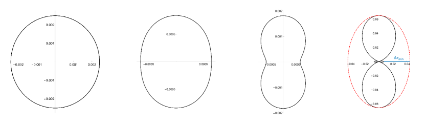
Figure 5: Orbits in the $(r(\tau)-r_{i},\phi(\tau))$ plane for initial radii (from left to right) $r_{i}/M=6.01,7,10,25$ in a single period $T$. For graphical reason in the first case the radial coordinate is obtained as $r(\tau)-6.025M$. In the last panel the blue line rapresents $\Delta r_{\rm min}$ mentioned in the main text.

We start with a particle initially at $r=r_{i}$ on a circular orbit, i.e.,

$$u_{0}^{\mu}=\left(\sqrt{\frac{r_{i}}{r_{i}-3M}},0,0,\frac{1}{r_{i}}\sqrt{\frac{M}{r_{i}-3M}}\right)\,,$$ (64)

and we integrate the geodesic equation up to $\tau\sim 10\lambda^{-1}$.

As the companion approaches its asymptotic location $R_{0}$, the particle is pulled to a slightly larger orbital radius, while the orbits becomes slightly eccentric, as shown in Fig. 4.

If we assume that the orbit is elliptic, we can extract the local maximum and minimum values of the radial coordinate to compute an eccentricity-like quantity

$$e=\sqrt{1-(r_{\rm min}/r_{\rm max})^{2}}\,,$$ (65)

as well as its period $T$. Specifically, these quantities are evaluated for a single period $T$ and extracted when the companion is almost steady, so at late times. Results are reported in Table 4. Note that $T$ is to a good precision the orbital period of a particle in circular motion, given by Kepler’s law. Not surprisingly, $e$ increases as the particle moves away from the BH and get closer to the companion. Specifically, it scales as

$$e\propto\left(\frac{r_{i}}{M}\right)^{1.8}\,.$$ (66)

In fact, the motion is not really eccentric in these coordinates. For large $r_{i}$, we find that the motion acquires a peanut-like shape, as shown in Fig. 5. If we take the $\phi=0$ direction as the apoapsis $r_{\rm min}$ direction, then deviations from a perfect elliptic shape are of order $\Delta r_{\rm min}/r_{\rm min}\sim 10^{-3}$ (blue line in the last panel of Figure 5). As a consequence, the eccentricity-like parameter $e$ can still be considered an adequate measure of deviation from circularity.

Likewise, both the period $T$ and the shapes of the orbits in Figure 5 are unaffected by the change in the final position. The only relevant difference is in the numerical values of $r_{\rm min}$ and $r_{\rm max}$, as well as in their ratio. In fact, as expected, these values become larger (smaller) if the companion is at $R_{0}/M=100$ ($300$). As a consequence, orbits have a larger (smaller) value of the parameter $e$, though its scaling with $r_{i}$ is still well described by Eq. (66). To be precise, the exponent is $1.71$ for $R_{0}=300$ and $1.88$ for $R_{0}=100$.

The final position of the particle, due to the presence of a companion, is dependent both on the strength of the perturbation and the initial radius. If we denote by $r_{\rm fin}$ the average value between $r_{\rm min}$ and $r_{\rm max}$, extracted when the companion is now steady, we find that for radii $r_{i}\geq 10M$ the displacement $\Delta r=r_{\rm fin}-r_{i}$ is given by

$$\frac{\Delta r}{r_{i}}\approx A\,\left(\frac{r_{i}}{M}\right)^{3}\,\epsilon$$ (67)

with the constant $A$ of order of unity.

V Discussion

The understanding of accretion disks or of the orbital motion of stars is a fundamental aspect in the interpretation of astrophysical observations. In addition, the location and properties of the the light ring around BHs are crucial in the understanding of the dynamics in the strong-field regime. Thus, peculiarities in motion in deep strong-field regions could indicate either new physics or simply the presence of an unseen companion Naoz et al. (2020). Motivated by this possibility, we studied the geodesic motion of both null and timelike orbits when tidal perturbations induced by an external companion are present.

There are several new features of tidally distorted BH geometries relative to BHs in isolation. When the orbital plane is orthogonal to that of the BH-companion, we were able to analytically quantify the linear deviations in the characteristic orbits induced by the companion. Specifically, with respect to the unperturbed configuration, the light ring has larger radius and orbital frequency, while the ISCO is located closer to the BH and, consequently, has a larger angular frequency. In this framework we also obtained the QNM frequencies for the $l=m=2$ modes and we found that the ringdown frequency (the damping rate) is shifted to a slightly larger (smaller) value with respect to that of a Schwarzschild BH.

Instead, studying the late-time behaviour of the field showed that the structure of the modes of such a geometry is noticeably different from that of a single BH and is instead typical of confined systems. These properties had already been observed previously Bernard et al. (2019). However, in order to correctly capture all the physical properties of the relaxation stage, it is necessary to construct a spacetime which correctly reproduces the asymptotic behaviour at infinity Bernard et al. (2019). Further investigations in this direction are left for future work.

On the other hand, when orbits lie in the same plane as that of the BH-companion system, one needs a numerical study. We showed that the light ring is still a closed orbit but with an elliptical shape characterized by eccentricity and axes proportional to $\epsilon$ (cf. Fig. 3). Timelike orbits displayed a similar behaviour but other effects took place as well. The companion induces a relaxing of the orbit of point particles, which moves toward larger radii and are tidally distorted as seen in Fig. 5. We also explored the possibility for the spacetime to admit static orbits and we found an expression for their initial radius $r_{s}$ in agreement with the Newtonian treatment of the problem.

References

- Flanagan and Hinderer (2008) E. E. Flanagan and T. Hinderer, Phys. Rev. D 77, 021502 (2008), arXiv:0709.1915 [astro-ph] .
- Dietrich et al. (2020) T. Dietrich, T. Hinderer, and A. Samajdar, (2020), arXiv:2004.02527 [gr-qc] .
- Gupta et al. (2020) P. K. Gupta, J. Steinhoff, and T. Hinderer, (2020), arXiv:2011.03508 [gr-qc] .
- Chrusciel et al. (2012) P. T. Chrusciel, J. Lopes Costa, and M. Heusler, Living Rev. Rel. 15, 7 (2012), arXiv:1205.6112 [gr-qc] .
- Cardoso and Gualtieri (2016) V. Cardoso and L. Gualtieri, Class. Quant. Grav. 33, 174001 (2016), arXiv:1607.03133 [gr-qc] .
- Cardoso et al. (2017) V. Cardoso, E. Franzin, A. Maselli, P. Pani, and G. Raposo, Phys. Rev. D 95, 084014 (2017), [Addendum: Phys.Rev.D 95, 089901 (2017)], arXiv:1701.01116 [gr-qc] .
- Sennett et al. (2017) N. Sennett, T. Hinderer, J. Steinhoff, A. Buonanno, and S. Ossokine, Phys. Rev. D 96, 024002 (2017), arXiv:1704.08651 [gr-qc] .
- Cardoso and Pani (2019) V. Cardoso and P. Pani, Living Rev. Rel. 22, 4 (2019), arXiv:1904.05363 [gr-qc] .
- Naoz et al. (2020) S. Naoz, C. M. Will, E. Ramirez-Ruiz, A. Hees, A. M. Ghez, and T. Do, Astrophys. J. Lett. 888, L8 (2020), arXiv:1912.04910 [astro-ph.GA] .
- Abuter et al. (2018) R. Abuter et al. (GRAVITY), Astron. Astrophys. 615, L15 (2018), arXiv:1807.09409 [astro-ph.GA] .
- Abuter et al. (2020) R. Abuter et al. (GRAVITY), Astron. Astrophys. 636, L5 (2020), arXiv:2004.07187 [astro-ph.GA] .
- Murray and Dermott (2000) C. D. Murray and S. F. Dermott, Solar System Dynamics (Cambridge University Press, 2000).
- Domingos et al. (2008) R. C. Domingos, R. Vilhena de Moraes, and D. A. P. Bertachini, Mathematical Problems in Engineering 2008 (2008), 10.1155/2008/763654.
- Chandrasekhar (1983) S. Chandrasekhar, The Mathematical Theory of Black Holes (Oxford University Press, New York, 1983).
- Cardoso et al. (2009) V. Cardoso, A. S. Miranda, E. Berti, H. Witek, and V. T. Zanchin, Phys. Rev. D 79, 064016 (2009), arXiv:0812.1806 [hep-th] .
- Cardoso et al. (2016) V. Cardoso, E. Franzin, and P. Pani, Phys. Rev. Lett. 116, 171101 (2016), arXiv:1602.07309 [gr-qc] .
- Yang (2021) H. Yang, (2021), arXiv:2101.11129 [gr-qc] .
- Nakashi and Igata (2019a) K. Nakashi and T. Igata, Phys. Rev. D 99, 124033 (2019a), arXiv:1903.10121 [gr-qc] .
- Nakashi and Igata (2019b) K. Nakashi and T. Igata, Phys. Rev. D 100, 104006 (2019b), arXiv:1908.10075 [gr-qc] .
- Assumpcao et al. (2018) T. Assumpcao, V. Cardoso, A. Ishibashi, M. Richartz, and M. Zilhao, Phys. Rev. D 98, 064036 (2018), arXiv:1806.07909 [gr-qc] .
- Bernard et al. (2019) L. Bernard, V. Cardoso, T. Ikeda, and M. Zilhão, Phys. Rev. D 100, 044002 (2019), arXiv:1905.05204 [gr-qc] .
- Daza et al. (2018) A. Daza, J. O. Shipley, S. R. Dolan, and M. A. Sanjuán, Phys. Rev. D 98, 084050 (2018), arXiv:1807.10741 [gr-qc] .
- Regge and Wheeler (1957) T. Regge and J. A. Wheeler, Phys. Rev. 108, 1063 (1957).
- Zerilli (1970) F. Zerilli, Phys. Rev. D 2, 2141 (1970).
- Berti et al. (2009) E. Berti, V. Cardoso, and A. O. Starinets, Class. Quant. Grav. 26, 163001 (2009), arXiv:0905.2975 [gr-qc] .
- Thorne (1980) K. Thorne, Rev. Mod. Phys. 52, 299 (1980).
- Zhang (1986) X. H. Zhang, Phys. Rev. D 34, 991 (1986).
- Binnington and Poisson (2009) T. Binnington and E. Poisson, Phys. Rev. D80, 084018 (2009), arXiv:0906.1366 [gr-qc] .
- Poisson and Will (1953) E. Poisson and C. Will, Gravity: Newtonian, Post-Newtonian, Relativistic (Cambridge University Press, Cambridge, UK, 1953).
- Cardoso et al. (2020) V. Cardoso, F. Duque, and T. Ikeda, (2020), arXiv:2001.01729 [gr-qc] .
- Leaver (1986) E. W. Leaver, Phys. Rev. D 34, 384 (1986).
- Yang et al. (2012) H. Yang, D. A. Nichols, F. Zhang, A. Zimmerman, Z. Zhang, and Y. Chen, Phys. Rev. D 86, 104006 (2012), arXiv:1207.4253 [gr-qc] .
- Cardoso and Pani (2017) V. Cardoso and P. Pani, Nat. Astron. 1, 586 (2017), arXiv:1709.01525 [gr-qc] .
- Cano et al. (2020) P. A. Cano, K. Fransen, and T. Hertog, Phys. Rev. D 102, 044047 (2020), arXiv:2005.03671 [gr-qc] .
- Brito et al. (2014) R. Brito, V. Cardoso, and P. Pani, Phys. Rev. D 89, 104045 (2014), arXiv:1405.2098 [gr-qc] .
- Leung et al. (1997) P. T. Leung, Y. T. Liu, W. M. Suen, C. Y. Tam, and K. Young, Phys. Rev. Lett. 78, 2894 (1997), arXiv:gr-qc/9903031 [gr-qc] .
- Barausse et al. (2014) E. Barausse, V. Cardoso, and P. Pani, Phys. Rev. D89, 104059 (2014), arXiv:1404.7149 [gr-qc] .
- Butikov (2002) E. I. Butikov, American Journal of Physics 70, 1001 (2002).
- Hjorth and Knudsen (1996) P. Hjorth and J. Knudsen, Elements of Newtonian mechanics (Springer Verlag, Germany, 1996).