Abstract

In Veltman’s original view, the Standard Model with a large Higgs particle mass $M_{h}\lesssim$ 1 TeV was the natural completion of the non-renormalizable Glashow model. In this sense, this mass was a second threshold for weak interactions, as the W mass was for the non-renormalizable 4-fermion V-A theory. Today, after the observation of the narrow scalar resonance with $m_{h}=$ 125 GeV, Veltman’s large $M_{h}$ seems to be ruled out. Yet, depending on the description of SSB in $\Phi^{4}$ theory, this is not necessarily true. In fact, besides the mass $m_{h}$ describing its quadratic shape, the effective potential might exhibit a much larger mass scale $M_{h}$ associated with the zero-point energy which determines its depth. This larger $M_{h}$ controls vacuum stability and, differently from $m_{h}$, would remain finite in units of the weak scale $\langle\Phi\rangle\sim$ 246.2 GeV for infinite ultraviolet cutoff. Lattice simulations of the propagator are consistent with this two-mass structure and lead to the estimate $M_{h}\sim 700$ GeV. In spite of its large mass, however, the heavier state would couple to longitudinal W’s with the same typical strength of the low-mass state and thus represent a relatively narrow resonance. In this way, such hypothetical resonance would naturally fit with some excess of 4-lepton events observed by ATLAS around 680 GeV. Analogous data from CMS are needed to confirm or disprove this interpretation. Implications of this two-mass structure for radiative corrections will also be discussed.

1. Introduction

In principle, there were many possible scenarios for the Higgs particle mass. At the extremes of the mass range one could consider two basically different options. The (minimal) supersymmetry, where the mass of the lightest Higgs scalar is $m_{h}\sim M_{w}$, and Veltman’s idea [1] of a large $M_{h}\lesssim 1$ TeV. In his view, incorporating the idea of Spontaneous Symmetry Breaking (SSB) [2, 3] with a large $M_{h}$, the Standard Model was the natural completion of the non-renormalizable Glashow model [4]. In this sense, he was speaking of a second threshold in weak interactions, just like with the W mass and the non-renormalizable 4-fermion V-A theory. Today, after the observation at LHC [5, 6] of the narrow scalar resonance with mass $m_{h}\sim 125$ GeV, Veltman’s large $M_{h}$ seems to be definitely ruled out.

However, this is not necessarily true. So far, only the gauge and Yukawa couplings of the 125 GeV resonance have been tested. The effects of a genuine scalar self-coupling $\lambda=3m^{2}_{h}/\langle\Phi\rangle^{2}$ are still below the accuracy of the measurements and an uncertainty about the origin of SSB still persists. Given this uncertainty, one may wonder about the traditional assumption that the Higgs field propagator has only one pole associated with the quadratic shape of the scalar potential at its minima. While Goldstone bosons are well understood, depending on the physical mechanisms which induce SSB, the broken-symmetry phase could display a richer pattern of scales and the Higgs field exhibit some yet undiscovered, heavier resonance of mass $M_{h}\gg m_{h}$. Veltman’s original view could then be realized albeit in a new, unexpected way.

About the origin of SSB, at the beginning the driving mechanism was just a classical potential with double-well shape. Later on, after Coleman and Weinberg [7], this classical potential was replaced by the effective potential $V_{\rm eff}(\varphi)$ which, in principle, includes the zero-point energy of all particles in the spectrum. But SSB could still be determined by the pure scalar sector if the other contributions to the vacuum energy were negligible. Then, as argued in refs.[8, 9], a series of logical steps leads to the idea of a Higgs propagator with more than one peak.

One should first follow those lattice simulations of $\Phi^{4}$ in 4D [10, 11, 12] indicating that SSB is a (weak) first-order phase transition. While in the presence of gauge bosons SSB is often described as a first-order transition, in pure $\Phi^{4}$ this requires to replace standard perturbation theory with some alternative scheme. A scheme where massless $\Phi^{4}$ (i.e. classically scale invariant) exhibits SSB so that the phase transition occurs earlier, when the quanta of the symmetric phase have a tiny but still positive mass squared. One then discovers that, in the two easily available alternative schemes (the simple 1-loop and/or Gaussian approximation), $V_{\rm eff}(\varphi)$ has two distinct mass scales [8, 9]: i) a mass $m^{2}_{h}$, defined by its quadratic shape at the minimum and  ii) a mass $M^{2}_{h}$ entering the zero-point energy which determines its depth. Always considered as being the same mass, in these approximations one finds instead $M^{2}_{h}\sim Lm^{2}_{h}\gg m^{2}_{h}$, where $L=\ln(\Lambda_{s}/M_{h})$ and $\Lambda_{s}$ is the ultraviolet cutoff of the scalar sector. Since vacuum stability depends on the much larger $M_{h}$, and not on $m_{h}$, SSB could originate within the pure scalar sector regardless of the other parameters of the theory (e.g. the vector boson and top quark mass).

It is obvious that quadratic shape and depth of the potential are different quantities. At a more formal level, one should recall that the derivatives of the effective potential produce (minus) the n-point functions at zero external momentum. Hence $m^{2}_{h}$, which is $V^{\prime\prime}_{\rm eff}(\varphi)$ at the minimum, is directly the 2-point, self-energy function $|\Pi(p=0)|$. On the other hand, the zero-point energy is (one-half of) the trace of the logarithm of the inverse propagator $G^{-1}(p)=(p^{2}-\Pi(p))$. Therefore, after subtracting constant terms and quadratic divergences, matching the 1-loop zero-point energy(“$zpe$”) gives the relation

$$zpe\sim-\frac{1}{4}\int^{p_{\rm max}}_{p_{\rm min}}{{d^{4}p}\over{(2\pi)^{4}}}\frac{\Pi^{2}(p)}{p^{4}}\sim-\frac{\langle\Pi^{2}(p)\rangle}{64\pi^{2}}\ln\frac{p^{2}_{\rm max}}{p^{2}_{\rm min}}\sim-\frac{M^{4}_{h}}{64\pi^{2}}\ln\frac{\Lambda^{2}_{s}}{M^{2}_{h}}$$ (1)

This shows that $M^{2}_{h}$ effectively includes the contribution of all momenta and reflects a typical average value $|\langle\Pi(p)\rangle|$ at larger $p^{2}$. A non-trivial momentum dependence of $\Pi(p)$ would then indicate the coexistence in the broken-symmetry phase of two kinds of “quasi-particles”, with masses $m_{h}$ and $M_{h}$, and thus closely resemble the two branches (phonons and rotons) in the energy spectrum of superfluid He-4 which is usually considered the non-relativistic analog of the broken phase.

Actually, due to their conceptual difference, the issue $m_{h}\neq M_{h}$ could be posed on a pure hypothetical basis, independent of any specific calculation. Then, a non uniform scaling of the two masses with $\Lambda_{s}$ could be deduced for consistency with the “triviality” of $\Phi^{4}$. This implies a continuum limit with a Gaussian set of Green’s functions and with just a massive free-field propagator. Therefore, with this constraint, besides the usual $m_{h}\to M_{h}$ limit, a consistent cutoff theory can also predict their non-uniform scaling when $\Lambda_{s}\to\infty$. The type of single-mass limit will then depend on the unit scale, $m_{h}$ or $M_{h}$, chosen for measuring momenta. Namely: a) $m_{h}$ is the unit scale so that $M_{h}$ and the higher branch simply decouple b) $M_{h}$ is the unit scale so that, when $\Lambda_{s}\to\infty$, the phase space of the lower branch becomes smaller and smaller until ideally shrinking to the zero-measure set $p_{\mu}=0$ which is transformed into itself under the Lorentz Group. This means that the lower branch merges into the vacuum state and the only remaining excitation is the higher branch with mass $M_{h}$, reproducing the usual picture of a massive fluctuation field for any $p_{\mu}\neq 0$.

Given this consistency with rigorous field-theoretical results, the existence of a two-mass structure in the cutoff theory was checked with lattice simulations of the scalar propagator [8] in the 4D Ising limit of the theory. This corresponds to a $\Phi^{4}$ with an infinite bare coupling $\lambda_{0}=+\infty$, as when sitting precisely at the Landau pole. For a given non-zero, low-energy coupling $\lambda\sim 1/L$, this represents the best possible definition of the local limit with a cutoff. Then, once $m^{2}_{h}$ is directly computed from the $p^{2}\to 0$ limit of $G(p)$ and $M^{2}_{h}$ is extracted from its behaviour at higher $p^{2}$, the lattice data are consistent with a transition between two different regimes and with the expected increasing logarithmic trend $M^{2}_{h}\sim Lm^{2}_{h}$.

If, for finite $\Lambda_{s}$, the scalar propagator really interpolates between two vastly different scales, by increasing the energy there should be a transition from a relatively low value, e.g. $m_{h}$=125 GeV, to a much larger $M_{h}$. At the same time, differently from $m_{h}$, the larger mass $M_{h}$ would remain finite in units of the weak scale $\langle\Phi\rangle\sim(G_{\rm Fermi}\sqrt{2})^{-1/2}\sim$ 246.2 GeV in the continuum limit. In fact, by expressing the proportionality relation in terms of some constant $c_{2}$, say

$$M^{2}_{h}=m^{2}_{h}L\cdot(c_{2})^{-1}$$ (2)

and replacing the leading-order estimate $\lambda\sim 16\pi^{2}/(3L)$ in the relation $\lambda=3m^{2}_{h}/\langle\Phi\rangle^{2}$, one obtains a proportionality relation through a constant $K$

$$M_{h}=K\langle\Phi\rangle$$ (3)

with $K\sim(4\pi/3)\cdot(c_{2})^{-1/2}$. Since, from a fit to the lattice propagator [8], we found $(c_{2})^{-1/2}=0.67\pm 0.01~{}({\rm stat})\pm 0.02~{}({\rm sys})$ this gives the leading-order estimate $M_{h}=690\pm 10~{}({\rm stat})\pm 20~{}({\rm sys})~{}{\rm GeV}$. Instead, with the next-to-leading $m_{h}-\langle\Phi\rangle$ relation and the same $c_{2}$, we obtained $M_{h}=750\pm 10~{}({\rm stat})\pm 20~{}({\rm sys})$ GeV [8]. The two values could then be summarized into a final estimate $M_{h}\sim 720\pm 30$ GeV which accounts for this theoretical uncertainty and updates the previous work of refs.[13, 14].

I emphasize that, by accepting the “triviality” of the theory in 4D, the cutoff-independent combination $3M^{2}_{h}/\langle\Phi\rangle^{2}=3K^{2}$ cannot represent a measure of observable interactions. This $3K^{2}=O(10)$, which is clearly quite distinct from the other coupling $\lambda=3m^{2}_{h}/\langle\Phi\rangle^{2}\sim 1/L$, should not be viewed as a coupling constant which produces observable interactions in the broken-symmetry phase. Instead, since $M_{h}$ reflects the magnitude of the vacuum energy density, it would be natural to consider $3K^{2}\sim\lambda L$ as a collective self-interaction of the vacuum condensate which persists in the $\Lambda_{s}\to\infty$ limit. This original view [15, 16] can intuitively be formulated in terms of a scalar condensate whose increasing density $\sim L$ [17] compensates for the decreasing strength $\lambda\sim 1/L$ of the two-body coupling. On the other hand $\lambda\sim 1/L$ remains as the appropriate coupling to describe the individual interactions of the elementary excitations of the vacuum, i.e. the Higgs field and the Goldstone bosons. In this way, consistently with the “triviality” of $\Phi^{4}$ theory, their interactions will become weaker and weaker for $\Lambda_{s}\to\infty$. On this basis, the heavier state would couple to longitudinal vector bosons with the same typical strength $\lambda=3m^{2}_{h}/\langle\Phi\rangle^{2}\sim 1/L$ of the low-mass state and would thus represent a relatively narrow resonance.

In the following, I will first resume in Sects. 2, 3 and 4 the main analytical and numerical arguments in favor of the $m_{h}-M_{h}$ picture. Later on, in Sects.5 and 6, I will concentrate on more phenomenological aspects and argue that the hypothetical, heavier $M_{h}$ would naturally fit with some excess of 4-lepton events observed by ATLAS around 680 GeV. Finally in the conclusive Sect.7, after a short summary, I will mention a work of van der Bij [18] where a Higgs field propagator with more than one peak was also considered. This brings in touch with the possible effects of a two-mass structure in radiative corrections.

2. SSB and the effective potential

To start with, let us recall the description of SSB as a second-order transition and follow the Particle Data Group (PDG) [19] where the scalar potential is expressed as

$$V_{\rm PDG}(\varphi)=-\frac{1}{2}m^{2}_{\rm PDG}\varphi^{2}+\frac{1}{4}\lambda_{\rm PDG}\varphi^{4}$$ (4)

By fixing $m_{\rm PDG}\sim$ 88.8 GeV and $\lambda_{\rm PDG}\sim 0.13$, this has a minimum at $|\varphi|=\langle\Phi\rangle\sim$ 246 GeV and quadratic shape $V^{\prime\prime}_{\rm PDG}(\langle\Phi\rangle)=$ (125 GeV)². As a built-in relation, the second derivative of the potential also determines its depth, i.e. the vacuum energy ${\cal E}_{\rm PDG}$

$${\cal E}_{\rm PDG}=-\frac{1}{2}m^{2}_{\rm PDG}\langle\Phi\rangle^{2}+\frac{1}{4}\lambda_{\rm PDG}\langle\Phi\rangle^{4}=-\frac{1}{8}(125~{}{\rm GeV}\langle\Phi\rangle)^{2}\sim-1.2\cdot 10^{8}~{}{\rm GeV}^{4}$$ (5)

But, as anticipated in the Introduction, recent lattice simulations of $\Phi^{4}$ in 4D [10, 11, 12] indicate instead a (weakly) first-order transition. SSB would then emerge as a true instability of the symmetric vacuum at $\varphi=0$. Its quanta have a tiny and still positive mass squared $V^{\prime\prime}_{\rm eff}(\varphi=0)=m^{2}_{\Phi}>0$ but nevertheless, below a critical value $0\leq m^{2}_{\Phi}<m^{2}_{c}$, their attractive, long-range interaction [17] can destabilize this symmetric vacuum. The lowest energy state of the massless theory at $m^{2}_{\Phi}=0$ would then correspond to the broken-symmetry phase, as suggested by Coleman and Weinberg [7] in their original 1-loop calculation.

In this interpretation of SSB, the dynamics of the symmetric phase represents the primary $\Phi^{4}$ sector and its degree of locality $\Lambda_{s}$ is the ultimate cutoff scale of the theory (as with the hard-sphere core of He-4 atoms in superfluid helium). We are thus lead to identify $\Lambda_{s}$ as the Landau pole where the bare coupling $\lambda_{0}\to+\infty$. This corresponds precisely to the Ising limit and provides the best possible definition of a local $\Phi^{4}$ theory for any non-zero low-energy coupling $\lambda\sim 1/\ln\Lambda_{s}\ll 1$ . This latter coupling is instead appropriate for low-energy physics, as in the original Coleman-Weinberg calculation of the effective potential for field values $|\varphi|\ll\Lambda_{s}$ . The Coleman-Weinberg calculation represents the simplest scheme which is consistent with a weak first-order picture. We will first reproduce below this well known computation and discuss afterward its general validity. After subtraction of constant terms and quadratic divergences, the effective potential is

$$V_{\rm eff}(\varphi)=\frac{\lambda}{4!}\varphi^{4}+\frac{\lambda^{2}}{256\pi^{2}}\varphi^{4}\left[\ln({\scriptstyle{\frac{1}{2}}}\lambda\varphi^{2}/\Lambda^{2}_{s})-\frac{1}{2}\right]$$ (6)

and its first few derivatives are

$$V^{\prime}_{\rm eff}(\varphi)=\frac{\lambda}{6}\varphi^{3}+\frac{\lambda^{2}}{64\pi^{2}}\varphi^{3}\ln({\scriptstyle{\frac{1}{2}}}\lambda\varphi^{2}/\Lambda^{2}_{s})$$ (7)

and

$$V^{\prime\prime}_{\rm eff}(\varphi)=\frac{\lambda}{2}\varphi^{2}+\frac{3\lambda^{2}}{64\pi^{2}}\varphi^{2}\ln({\scriptstyle{\frac{1}{2}}}\lambda\varphi^{2}/\Lambda^{2}_{s})+\frac{\lambda^{2}\varphi^{2}}{32\pi^{2}}$$ (8)

By introducing the mass squared parameter $M^{2}(\varphi)\equiv{\scriptstyle{\frac{1}{2}}}\lambda\varphi^{2}$, the same potential can be expressed as a classical background + zero-point energy of a particle with mass $M(\varphi)$, i.e.

$$V_{\rm eff}(\varphi)=\frac{\lambda\varphi^{4}}{4!}-\frac{M^{4}(\varphi)}{64\pi^{2}}\ln\frac{\Lambda^{2}_{s}\sqrt{e}}{M^{2}(\varphi)}$$ (9)

Thus, non-trivial minima of $V_{\rm eff}(\varphi)$ occur at those points $\varphi=\pm v$ where

$$M^{2}_{h}={{\lambda v^{2}}\over{2}}=\Lambda^{2}_{s}\exp(-{{32\pi^{2}}\over{3\lambda}})$$ (10)

with a quadratic shape

$$m^{2}_{h}\equiv V^{\prime\prime}_{\rm eff}(\pm v)=\frac{\lambda^{2}v^{2}}{32\pi^{2}}=\frac{\lambda}{16\pi^{2}}M^{2}_{h}\sim\frac{M^{2}_{h}}{L}\ll M^{2}_{h}$$ (11)

where $L\equiv\ln\frac{\Lambda_{s}}{M_{h}}$. Notice that the energy density depends on $M_{h}$ and not on $m_{h}$, because

$${\cal E}=V_{\rm eff}(\pm v)=-\frac{M^{4}_{h}}{128\pi^{2}}$$ (12)

therefore the critical temperature at which symmetry is restored, $k_{B}T_{c}\sim M_{h}$, and the stability of the broken phase depends on the larger $M_{h}$ and not on the smaller $m_{h}$.

Now, one may object to the above straightforward minimization procedure that the 1-loop calculation is just the first term of an infinite series and should be further “improved”. As it is well known, in this conventional view, the 1-loop minimum disappears and one would again predict a second-order transition, just the result that we know to be in contrast with most recent lattice simulations. Therefore, one should look at the calculation in the different perspective of Eq.(9). This has the qualitatively different meaning of a classical background + zero-point energy with a $\varphi-$dependent mass and, as such, is consistent by itself without any need of being further improved.

To confirm the validity of this interpretation, one can compare with other approximation schemes, for instance the Gaussian approximation [25, 26] which has a variational nature and explores the Hamiltonian in the class of the Gaussian functional states. It also represents a very natural alternative because, at least in the continuum limit, a Gaussian structure of Green’s functions fits with the generally accepted “triviality” of the theory in 4D. This other calculation produces a result in agreement with the one-loop potential [15, 16]. This is not because there are no non-vanishing corrections beyond 1-loop; there is actually an infinite resummation of terms. The point, however, is that those additional terms do not alter the functional form of the result which is the same as in Eq.(9)

$$V^{G}_{\rm eff}(\varphi)=\frac{\hat{\lambda}\varphi^{4}}{4!}-\frac{\Omega^{4}(\varphi)}{64\pi^{2}}\ln\frac{\Lambda^{2}_{s}\sqrt{e}}{\Omega^{2}(\varphi)}$$ (13)

with

$$\hat{\lambda}=\frac{\lambda}{1+\frac{\lambda}{16\pi^{2}}\ln\frac{\Lambda_{s}}{\Omega(\varphi)}}~{}~{}~{}~{}~{}~{}~{}~{}~{}~{}~{}~{}{\rm and}~{}~{}~{}~{}~{}~{}~{}~{}~{}~{}~{}~{}~{}~{}~{}~{}~{}\Omega^{2}(\varphi)=\frac{\hat{\lambda}\varphi^{2}}{2}$$ (14)

This explains why the one-loop potential can also admit a non-perturbative interpretation. It is the prototype of the Gaussian and of the infinite number of “post-gaussian” calculations [27, 28] where higher-order contributions are effectively reabsorbed into the same basic structure: classical background + zero-point energy with a $\varphi-$dependent mass.

3. Eliminating $\Lambda_{s}$ in the $M_{h}-\langle\Phi\rangle$ relation

The effective potential of Sect.2 provides a different path to renormalization. Since, for any non-zero $\lambda$, there is a finite Landau pole, one could in fact consider the whole set of pairs ($\Lambda_{s}$,$\lambda$),($\Lambda^{\prime}_{s}$,$\lambda^{\prime}$), ($\Lambda^{\prime\prime}_{s}$,$\lambda^{\prime\prime}$)…with different Landau poles and corresponding low-energy couplings. By considering this whole set of parameters, and imposing some symmetry principle, one can minimize the influence of the cutoff on observable quantities and even consider the $\Lambda_{s}\to\infty$ limit.

The basic constraint on the equivalent ($\Lambda_{s}$,$\lambda$) pairs, consists in requiring the same vacuum energy Eq.(12), or equivalently the same mass scale Eq.(10), namely

$$\left(\Lambda_{s}\frac{\partial}{\partial\Lambda_{s}}+\Lambda_{s}\frac{\partial\lambda}{\partial\Lambda_{s}}\frac{\partial}{\partial\lambda}\right){\cal E}(\lambda,\Lambda_{s})=0$$ (15)

With the definition

$$\Lambda_{s}\frac{\partial\lambda}{\partial\Lambda_{s}}\equiv-\beta(\lambda)=-\frac{3\lambda^{2}}{16\pi^{2}}+O(\lambda^{3})$$ (16)

this gives $|{\cal E}|\sim{\cal I}^{4}_{1}$, where ${\cal I}_{1}$ is the first RG-invariant

$${\cal I}_{1}=M_{h}=\Lambda_{s}\exp({\int^{\lambda}\frac{dx}{\beta(x)}})\sim\Lambda_{s}\exp(-{{16\pi^{2}}\over{3\lambda}})$$ (17)

The above relations derive from the more general invariance of the effective potential in the three-dimensional space ($\varphi$, $\lambda$, $\Lambda_{s}$)

$$\left(\Lambda_{s}\frac{\partial}{\partial\Lambda_{s}}+\Lambda_{s}\frac{\partial\lambda}{\partial\Lambda_{s}}\frac{\partial}{\partial\lambda}+\Lambda_{s}\frac{\partial\varphi}{\partial\Lambda_{s}}\frac{\partial}{\partial\varphi}\right)V_{\rm eff}(\varphi,\lambda,\Lambda_{s})=0$$ (18)

In fact, at the minima $\varphi=\pm v$, where $(\partial V_{\rm eff}/\partial\varphi)=0$, Eq.(15) is a direct consequence of Eq.(18). Another consequence of this analysis is that, besides a first invariant mass scale ${\cal I}_{1}=M_{h}$, by introducing an anomalous dimension for the vacuum field

$$\Lambda_{s}\frac{\partial\varphi}{\partial\Lambda_{s}}\equiv\gamma(\lambda)\varphi$$ (19)

there is a second invariant, namely

$${\cal I}_{2}(\varphi)=\varphi\exp({\int^{\lambda}dx\frac{\gamma(x)}{\beta(x)}})$$ (20)

which introduces a particular normalization of $\varphi$. This had to be expected because from Eq.(10) the cutoff-independent combination is $\lambda v^{2}\sim M^{2}_{h}={\cal I}^{2}_{1}$ and not $v^{2}$ itself implying $\gamma=\beta/(2\lambda)$. This particular definition of the average vacuum field is then the natural candidate to represent the weak scale [8]

$${\cal I}_{2}(v)=\langle\Phi\rangle\sim 246.2~{}{\rm GeV}$$ (21)

so that the minimization of the effective potential can be expressed as a proportionality relation of the two invariants ${\cal I}_{1}$ and ${\cal I}_{2}$ through some constant $K$, i.e.

$$M_{h}=K\langle\Phi\rangle$$ (22)

On the other hand, the second derivative at the minima, $m^{2}_{h}\equiv(\partial^{2}V_{\rm eff}/\partial\varphi^{2})$ at $\varphi=\pm v$, remains as a cutoff-dependent quantity.

With such guiding principle from the effective potential, one deduces that $M_{h}$ and $\langle\Phi\rangle$ scale uniformly with $\Lambda_{s}$. The constant $K$ could then be extracted from a lattice simulation of the propagator, by combining the $M_{h}/m_{h}$ ratio with a theoretical $m_{h}-\langle\Phi\rangle$ relation. The main ingredients of this analysis will be reported in Sect.4.

4. Lattice simulation of the propagator

To show that the existence of two mass scales in the broken phase is not just speculation, let us now compare with lattice simulations of the propagator. These were performed [8] in the 4D Ising limit of the theory which has always been considered a convenient laboratory to exploit the non-perturbative aspects of the theory. As anticipated, it corresponds to a $\Phi^{4}$ with an infinite bare coupling $\lambda_{0}=+\infty$, as if one were sitting precisely at the Landau pole. In this sense, for any finite cutoff $\Lambda_{s}$, it provides the best definition of the local limit for a given non-zero, low-energy coupling $\lambda\sim 1/L$ (where $L=\ln(\Lambda_{s}/M_{h})$).

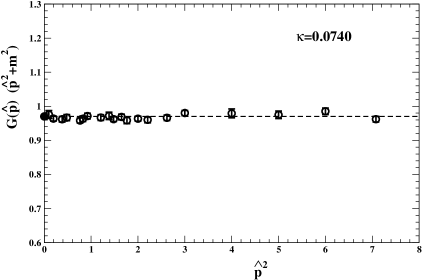
Figure 1: The lattice data of ref.[8] for the re-scaled propagator in the symmetric phase at $\kappa=0.074$ as a function of the square lattice momentum ${\hat{p}}^{2}$. The fitted mass from high ${\hat{p}}^{2}$, $m_{\rm{latt}}=0.2141(28)$, describes well the data down to ${\hat{p}}=0$. The dashed line indicates the value of $Z_{\rm{prop}}=0.9682(23)$ and the ${\hat{p}}=0$ point is $2\kappa\chi m^{2}_{\rm{latt}}=0.9702(91)$.

Let us start from the traditional Euclidean lattice action of $\Phi^{4}$ theory

$$S=\sum_{x}\left[\frac{1}{2}\sum^{4}_{\mu=1}(\partial_{\mu}\Phi_{0})^{2}+\frac{1}{2}m^{2}_{0}\Phi^{2}_{0}(x)+\frac{\lambda_{0}}{4!}\Phi^{4}_{0}(x)\right]$$ (23)

where $\partial_{\mu}\Phi_{0}=\Phi_{0}(x+\hat{\mu})-\Phi_{0}(x)$ and the lattice spacing is taken $a=1$. Analogously, all masses are given in units of $1/a$ and the cutoff is $\Lambda_{s}=\pi/a$. In this action, let us perform the following changes of variables [29] $\Phi_{0}=\sqrt{2\kappa}\Phi$, $m^{2}_{0}=(1-2g)/\kappa-8$ and $\lambda_{0}=6g/\kappa^{2}$ so that we obtain

$$S=\sum_{x}\left[-2\kappa\sum^{4}_{\mu=1}\Phi(x+\hat{\mu})\Phi(x)+\Phi^{2}(x)+g(\Phi^{2}(x)-1)^{2}\right]$$ (24)

Then, for $\lambda_{0}\to+\infty$, the lattice field can only take the values $\Phi(x)=\pm 1$ and one gets the Ising limit

$$S_{Ising}=-2\kappa\sum_{x}\sum^{4}_{\mu=1}\Phi(x+\hat{\mu})\Phi(x)$$ (25)

the broken-symmetry phase corresponding to $\kappa>\kappa_{c}$, with $\kappa_{c}=0.0748474(3)$ [10, 11]. With this lattice action, we computed the lattice field vacuum expectation value

$$v=\langle|\Phi|\rangle\quad,\quad\Phi\equiv\frac{1}{V_{4}}\sum_{x}\Phi(x)$$ (26)

and the connected propagator

$$G(x)=\langle\Phi(x)\Phi(0)\rangle-v^{2}$$ (27)

where $\langle...\rangle$ denotes averaging over the lattice configurations.

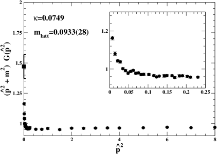
Figure 2: The propagator data of ref.[8], for $\kappa=0.0749$, rescaled with the lattice mass $M_{h}\equiv m_{\rm{latt}}=0.0933(28)$ obtained from the fit to all data with ${\hat{p}}^{2}>0.1$. The peak at $p=0$ is $M^{2}_{h}/m^{2}_{h}=1.47(9)$ as computed from the fitted $M_{h}$ and $m_{h}=(2\kappa\chi)^{-1/2}=0.0769(8)$.

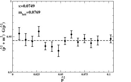
Figure 3: The propagator data of ref.[8] at $\kappa=0.0749$ for ${\hat{p}}^{2}<0.1$. The lattice mass used here for the rescaling was fixed at the value $m_{h}=(2\kappa\chi)^{-1/2}=0.0769(8)$.

By computing the Fourier transformed connected propagator as function of the lattice momentum $\hat{p}_{\mu}=2\sin p_{\mu}/2$, the extraction of $m^{2}_{h}$ is straightforward because its inverse is just the zero-momentum propagator, or susceptibility $\chi$

$$2\kappa\chi\equiv 2\kappa G(p=0)=\frac{1}{m^{2}_{h}}$$ (28)

Instead, to extract $M_{h}$ the propagator data were first fitted to the 2-parameter form

$$G_{\rm{fit}}(p)=\frac{Z_{\rm{prop}}}{{\hat{p}}^{2}+m^{2}_{\rm{latt}}}$$ (29)

in terms of the squared lattice momentum ${\hat{p}}^{2}$. The data were then re-scaled by $({\hat{p}}^{2}+m^{2}_{\rm{latt}})$ so that deviations from a flat plateau are immediately visible. This defines the standard single-particle mass and the difference from unity of the height of the plateau, which is $Z_{\rm{prop}}$, measures the residual coupling to multi-particle states.

The results in Fig.1 for $\kappa=0.074$, i.e. close to the critical point but still in the symmetric phase, show that, there, a single lattice mass works remarkably well in the whole range of momentum down to $p=0$. Thus single-particle states and multi-particles states are very weakly coupled in the whole momentum range. At least with a lattice mass of about 0.2, one is then close enough to the “trivial” continuum limit of $\Phi^{4}$ in 4D.

According to the standard point of view, in the broken phase there should be no particular difference. However, it was already observed in refs.[30] and [29] that, in this case, the mass from the higher-momentum fit cannot describe the data in the $p\to 0$ limit where the deviations from constancy become highly significant. As a further check, one more simulation was performed in ref. [8] on a large $76^{4}$ lattice for $\kappa=0.0749$, which is even closer to the critical point. As one can see from Fig.2, the mass parameter $m_{\rm{latt}}\equiv M_{h}$, obtained from the fit to the propagator for ${\hat{p}}^{2}>0.1$ cannot reproduce the data for ${\hat{p}}^{2}<0.1$. In this low-momentum range, in fact, the data select a smaller mass, which is very close to the inverse susceptibility $m_{h}=(2\kappa\chi)^{-1/2}=0.0769(8)$, see Fig.3.

The difference between $m_{h}$ and $M_{h}$ determines zero-momentum peaks, see Fig.2, which increase for $\kappa\to\kappa_{c}$. The observed values, $M^{2}_{h}/m^{2}_{h}=$1.24(5), 1.31(5), 1.47(9), respectively for $\kappa=$ 0.0751, 0.07504, 0.0749 [8], are consistent with the expected logarithmic trend $M^{2}_{h}=Lm^{2}_{h}(c_{2})^{-1}$ in Eq.(2), so that, as anticipated in the Introduction, one can fit these data and obtain $(c_{2})^{-1/2}=0.67\pm 0.01~{}({\rm stat})\pm 0.02~{}({\rm sys})$. With this value, and the leading-order estimate $\lambda=16\pi^{2}/(3L)$ in the relation $\lambda=3m^{2}_{h}/\langle\Phi\rangle^{2}$, one finds $M_{h}=690\pm 10~{}({\rm stat})\pm 20~{}({\rm sys})~{}{\rm GeV}$. Instead, with the next-to-leading $m_{h}-\langle\Phi\rangle$ relation and the same $c_{2}$, we obtained $M_{h}=750\pm 10~{}({\rm stat})\pm 20~{}({\rm sys})$ GeV [8]. The two values were then summarized into a final estimate $M_{h}\sim 720\pm 30$ GeV which accounts for the theoretical uncertainty and updates the previous work of refs.[13, 14].

5. The role of $m_{h}$ and $M_{h}$ in the observable interactions

The lattice simulations in the previous section, supporting the idea of a scalar propagator which smoothly interpolates between a mass scale $m_{h}$ and much larger $M_{h}$ with $M^{2}_{h}\sim Lm^{2}_{h}$, are consistent with the physical picture deduced from the effective potential. To understand the interplay of the two masses and their role in the observable processes, it is convenient to first follow ref.[31] where the phenomenology of a heavy but weakly interacting Higgs resonance was first considered.

Differently from here, where $m_{h}$ and $M_{h}$ are assumed to coexist, in ref.[31] one was adopting the ideal single-mass limit b) of the Introduction which (with the exception of the Lorentz-invariant, zero-measure set $p_{\mu}=0$) effectively reproduces a standard propagator with mass $M_{h}$. However, the problem was the same considered here: a $\Lambda_{s}-$independent scaling law $M_{h}=K\langle\Phi\rangle$. This opens a corner of parameter space, namely large $K$ but $M_{h}\ll\Lambda_{s}$, that does not exist in the conventional view. But, for this reason, the constant $3K^{2}$ is now basically different from the coupling $\lambda$ defined through the $\beta-$function

$$\ln\frac{\mu}{\Lambda_{s}}=\int^{\lambda}_{\lambda_{0}}~{}\frac{dx}{\beta(x)}$$ (30)

For $\beta(x)=3x^{2}/(16\pi^{2})+O(x^{3})$, whatever the contact coupling $\lambda_{0}$ at the asymptotically large $\Lambda_{s}$, at finite scales $\mu\sim M_{h}$ this gives $\lambda\sim 16\pi^{2}/(3L)$ with $L=\ln(\Lambda_{s}/M_{h})$. As anticipated, this $\lambda$ (and not the $\Lambda_{s}-$ independent $3K^{2}$) is the appropriate coupling to describe the infinitesimal interactions of the fluctuations of the broken phase.

Defining $M_{w}=g_{\rm gauge}\langle\Phi\rangle/2$ and with the notations of [32], a convenient parametrization [31] of these residual interactions in the scalar potential is ($r=M^{2}_{h}/4M^{2}_{w}=K^{2}/g^{2}_{\rm gauge}$)

$$U_{\rm scalar}=\frac{1}{2}M^{2}_{h}h^{2}+\epsilon_{1}rg_{\rm gauge}M_{w}h(\chi^{a}\chi^{a}+h^{2})+\frac{1}{8}\epsilon_{2}rg^{2}_{\rm gauge}(\chi^{a}\chi^{a}+h^{2})^{2}$$ (31)

The two parameters $\epsilon_{1}$ and $\epsilon_{2}$, which are usually set to unity, account for $\lambda\neq 3K^{2}$, i.e.

$$\epsilon^{2}_{1}=\epsilon_{2}=\frac{\lambda}{3K^{2}}\sim 1/L$$ (32)

But what about the full gauge theory? At first sight, the original calculation [33] in the unitary gauge could give the impression that $W_{L}W_{L}$ scattering is indeed governed by the large coupling $3K^{2}=3M^{2}_{h}/\langle\Phi\rangle^{2}$. To find the answer, let us recall the basics of that calculation. One starts from a tree-level amplitude $A_{0}$ which is formally $O(g^{2}_{\rm gauge})$ but ends up with

$$A_{0}(W_{L}W_{L}\to W_{L}W_{L})\sim\frac{3M^{2}_{h}g^{2}_{\rm gauge}}{4M^{2}_{w}}=3K^{2}$$ (33)

Here the factor $g^{2}_{\rm gauge}$ comes from the vertices. The $1/M^{2}_{w}$ derives from the external longitudinal polarizations $\epsilon^{(L)}_{\mu}\sim(k_{\mu}/M_{w})$ and $M^{2}_{h}$ emerges after expanding the propagator

$$\frac{1}{s-M^{2}_{h}}\to\frac{1}{s}(1+\frac{M^{2}_{h}}{s}+...)$$ (34)

While the leading $1/s$ contribution cancels against a similar term from the other diagrams (which otherwise would give an amplitude growing with $s$), the $M^{2}_{h}$ from the 2nd-order term is effectively “promoted” to coupling constant reproducing the same result of a pure $\Phi^{4}$ with contact coupling $\lambda_{0}=3K^{2}$ at some large scale $\Lambda_{s}$.

However, in $\Phi^{4}$, this is just the tree approximation with the same coupling at all momentum scale. To find the $\chi\chi\to\chi\chi$ amplitude at some scale $\mu$, we should instead use Eq.(30) and let the coupling evolve, from $\lambda_{0}$ to $\lambda$, as previously done in Eq.(31), i.e.

$$A(\chi\chi\to\chi\chi)\Big{|}_{g_{\rm gauge}=0}\sim\lambda\sim\frac{1}{\ln(\Lambda_{s}/\mu)}$$ (35)

Thus, recalling that the Equivalence Theorem is valid to all orders in the scalar self-interactions but to lowest order in $g_{\rm gauge}$ [34, 35, 36], we obtain the result anticipated in the Introduction

$$A(W_{L}W_{L}\to W_{L}W_{L})=[1+O(g^{2}_{\rm gauge})]~{}A(\chi\chi\to\chi\chi)\Big{|}_{g_{\rm gauge}=0}=O(\lambda)$$ (36)

This analysis, from our present perspective where $m_{h}$ and $M_{h}$ coexist and could be experimentally determined, shows that at $\mu\sim M_{h}$ the supposed strong interactions proportional to $\lambda_{0}=3K^{2}$ are actually controlled by the much smaller coupling

$$\lambda=\frac{3m^{2}_{h}}{\langle\Phi\rangle^{2}}=3K^{2}~{}\frac{m^{2}_{h}}{M^{2}_{h}}\sim 1/L$$ (37)

Analogously, the conventional very large width into longitudinal vector bosons computed with $\lambda_{0}=3K^{2}$, say $\Gamma^{\rm conv}(M_{h}\to W_{L}W_{L})\sim M^{3}_{h}/\langle\Phi\rangle^{2}$, should instead be rescaled by $\epsilon_{1}^{2}=(\lambda/3K^{2})=m^{2}_{h}/M^{2}_{h}$. This gives

$$\Gamma(M_{h}\to W_{L}W_{L})\sim\frac{m^{2}_{h}}{M^{2}_{h}}~{}\Gamma^{\rm conv}(M_{h}\to W_{L}W_{L})\sim M_{h}~{}\frac{m^{2}_{h}}{\langle\Phi\rangle^{2}}$$ (38)

where $M_{h}$ indicates the available phase space in the decay and ${m^{2}_{h}}/{\langle\Phi\rangle^{2}}$ the interaction strength. Therefore, it is through the decays of the heavier state that the coupling $\lambda=3m^{2}_{h}/\langle\Phi\rangle^{2}$ could become visible, thus confirming that $m_{h}$ and $M_{h}$ represent excitations of the same field.

6. Comparison with 4-lepton data

Suppose to take seriously the idea of a second heavier excitation of the Higgs field with mass $M_{h}\sim$ 700 GeV. Are there experimental indications for such resonance? Furthermore, what kind of phenomenology should we expect? Finally, what about the identification $m_{h}\sim$ 125 GeV, implicitly assumed for our lower mass scale? In the following, I will summarize the results of ref.[37] where these questions were addressed in connection with a certain excess of 4-lepton events observed by ATLAS [38, 39] for invariant mass $\mu_{4l}\sim$ 700 GeV ($l=e,\mu$).

Of course, the 4-lepton channel is just one possible decay channel and, for a comprehensive analysis, one should also look at the other final states. For instance, at the 2-photon channel that, in the past, has been showing some intriguing signal for the close energy of 750 GeV. However, the 4-lepton channel is experimentally clean and, for this reason, is considered the “golden” channel for a heavy Higgs resonance. Moreover, the bulk of the effect can be analyzed at an elementary level. Thus it makes sense to start from here.

The main new aspect is the strong reduction of the conventional width in Eq.(38). For $M_{h}=$ 700 GeV, where $\Gamma^{\rm conv}(M_{h}\to ZZ)\sim 56.7~{}{\rm GeV}$ [40, 41], fixing $m_{h}=125$ GeV gives

$$\Gamma(M_{h}\to ZZ)\sim\frac{m^{2}_{h}}{(700~{}{\rm GeV})^{2}}~{}56.7~{}{\rm GeV}\sim 1.8~{}{\rm GeV}$$ (39)

Afterward, by maintaining the other contributions for $M_{h}=$ 700 GeV [40, 41]

$$\Gamma(M_{h}\to{\rm fermions+gluons+photons...})\sim 28~{}{\rm GeV}$$ (40)

and with the same ratio $\Gamma(M_{h}\to WW)/\Gamma(M_{h}\to ZZ)\sim$ 2.03, we find a total width

$$\Gamma(M_{h}\to all)\sim 28~{}{\rm GeV}+3.03~{}\Gamma(M_{h}\to ZZ)\sim 33.5~{}{\rm GeV}$$ (41)

and a fraction $B(M_{h}\to ZZ)\sim(1.8~{}/~{}33.5)\sim 0.054$.

Now, the production cross section $\sigma(pp\to M_{h})$. Here the main contributions are the basic Gluon-Gluon Fusion (GGF) and Vector-Boson Fusion (VBF) processes, where two gluons or two vector bosons $VV$ ($WW$ or $ZZ$) fuse to produce the heavy state $M_{h}$, i.e.

$$\sigma(pp\to M_{h})\sim\sigma(pp\to M_{h})_{\rm GGF}+\sigma(pp\to M_{h})_{\rm VBF}$$ (42)

For the GGF term I will consider two estimates: $\sigma(pp\to M_{h})_{\rm GGF}=800(80)$ fb from ref.[40] and $\sigma(pp\to M_{h})_{\rm GGF}=1078(150)$ fb from ref.[41]. These refer to $\sqrt{s}=$ 14 TeV and should be rescaled by about $-12\%$ for $\sqrt{s}=$ 13 TeV.

Table 1: For $M_{h}=$ 700 GeV and $m_{h}=$ 125 GeV, we report our predictions for the peak cross section $\sigma_{R}(pp\to 4l)$ and the number of events at two values of the luminosity. The two total cross sections are our extrapolation to $\sqrt{s}=$ 13 TeV of the values in [40] and [41] for $\sqrt{s}=$ 14 TeV. As explained in the text, only the GGF mechanism is relevant in our model.

$\sigma(pp\to M_{h})$	$\sigma_{R}(pp\to 4l)$	$n_{\rm 4l}$ (36.1$fb^{-1})$	$n_{\rm 4l}$(139$fb^{-1})$
700(70) fb	0.17(2) fb	$6.0\pm 0.6$	$23.2\pm 2.3$
950(150) fb	0.23(4) fb	$8.1\pm 1.3$	$31.5\pm 5.0$

About VBF, I observe that the $VV\to M_{h}$ process is the inverse of the $M_{h}\to VV$ decay so that $\sigma(pp\to M_{h})_{\rm VBF}$ can be expressed [42] as a convolution with the parton densities of the same Higgs resonance decay width. Thus with a large $3K^{2}$ coupling to longitudinal $W$’s and $Z$’s and conventional width $\Gamma^{\rm conv}(M_{h}\to WW+ZZ)\sim$ 172 GeV, the VBF mechanism would become sizeable. But this coupling is not present in our picture, where instead $\Gamma(M_{h}\to WW+ZZ)\sim$ 5.5 GeV. Therefore, the VBF will correspondingly be reduced from its conventional estimate $\sigma^{\rm conv}(pp\to M_{h})_{\rm VBF}=250\div 300$ fb by the small ratio (5.5 / 172)$\sim$ 0.032. This gives $\sigma(pp\to M_{h})_{\rm VBF}~{}\lesssim 10~{}$ fb and can be neglected.

In the end, for a relatively narrow resonance the effects of its virtuality should be small. Thus one can approximate the resonance cross section by on-shell branching ratios as

$$\sigma_{R}(pp\to 4l)\sim\sigma(pp\to M_{h})\cdot B(M_{h}\to ZZ)\cdot 4B^{2}(Z\to l^{+}l^{-})$$ (43)

Altogether, for $B(M_{h}\to ZZ)\sim$ 0.054 and $4B^{2}(Z\to l^{+}l^{-})\sim 0.0045$, the expected peak cross section and numbers of events (for efficiency $\sim$ 0.98) are reported in Table 1.

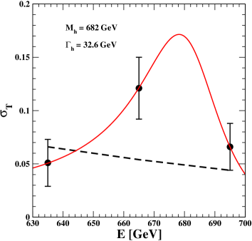
Figure 4: For $M_{h}=$ 682 GeV and $\Gamma_{h}=$ 32.6 GeV, a fit (in red) with Eq.(44) to the ATLAS data converted into cross sections in fb (the black dots). The fitted parameters are $\sigma_{R}=0.154\pm 0.054$ fb and $\sigma_{B}=0.009^{+0.017}_{-0.008}$ fb, or total fitted background $N^{\rm fit}_{B}=4^{+7}_{-4}$. Errors from fit give $\chi^{2}=$ 2.41 with $\chi^{2}_{\rm min}=0$. The dashed line is ATLAS background estimate.

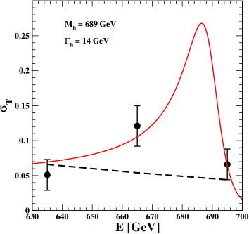
Figure 5: As in Fig.4 for $M_{h}=$ 689 GeV and $\Gamma_{h}=$ 14 GeV. Fitted parameters are $\sigma_{R}=0.19^{+0.16}_{-0.13}$ fb and $\sigma_{B}=0.04^{+0.01}_{-0.03}$ fb, or total fitted background $N^{\rm fit}_{B}=16^{+4}_{-12}$. Errors from fit give $\chi^{2}=$ 2.41 with $\chi^{2}_{\rm min}=1$. The dashed line is ATLAS background estimate.

For the smaller statistics of 36.1 fb^-1, see Fig.4a of [38], these predictions can be directly compared, and are well consistent, with the measured value $n_{\rm 4l}\sim(6\pm 3)$ for $\mu_{\rm 4l}=$ 700 GeV. Instead, to compare with the larger ATLAS sample [39] of 139 fb^-1 a different treatment is needed. In fact, in their Fig.2d there are now three points in the relevant energy region: at $\mu_{\rm 4l}\sim 635(15)$ GeV, where $n_{\rm 4l}\sim 7.0\pm 3.0$, at $\mu_{\rm 4l}\sim 665(15)$ GeV, where $n_{\rm 4l}\sim 16.5\pm 4.0$, and at $\mu_{\rm 4l}\sim 695(15)$ GeV, where $n_{\rm 4l}\sim 9.0^{+2.2}_{-3.0}$. Therefore, by defining $\mu_{4l}=E$ and $s=E^{2}$, we have assumed that these 4-lepton events derive from the interference of a resonating amplitude $A^{R}(s)\sim 1/(s-M^{2}_{R})$ and a slowly varying background $A^{B}(s)$. For positive interference below peak, setting $M^{2}_{R}=M^{2}_{h}-iM_{h}\Gamma_{h}$, this gives a total cross section

$$\sigma_{T}=\sigma_{B}-\frac{2(s-M^{2}_{h})~{}\Gamma_{h}M_{h}}{(s-M^{2}_{h})^{2}+(\Gamma_{h}M_{h})^{2}}~{}\sqrt{\sigma_{B}\sigma_{R}}+\frac{(\Gamma_{h}M_{h})^{2}}{(s-M^{2}_{h})^{2}+(\Gamma_{h}M_{h})^{2}}~{}\sigma_{R}$$ (44)

where, in principle, both the average background $\sigma_{B}$ and the resonating $\sigma_{R}$ could be treated as free parameters. By converting event numbers into cross sections, the best fit is at $M_{h}=$ 682 GeV, see Fig.4. Since in our model, for small changes of the mass, $\Gamma_{h}$ varies linearly with $M_{h}$, the width was constrained by the relation $(\Gamma_{h}/M_{h})=(33.5/700)$. ATLAS estimate of the background is also shown as a dashed line.

With this theoretical input the fit yields a small average background $\sigma_{B}=0.009^{+0.017}_{-0.008}$ fb, equivalent to total background events $N^{\rm fit}_{B}=4^{+7}_{-4}$, and a $\sigma_{R}$ consistent with Table 1. Therefore, if the observed number of events $N_{\rm obs}\sim 32\pm 7$ is expressed as $N_{\rm obs}=\Delta N+N_{B}$ the fit would give a minimum number of extra non-background events $(\Delta N)^{\rm fit}\sim 21\pm 7$, i.e. a genuine non-zero signal at the 3-sigma level. To better understand the relation between strength of the signal and resonance width, I have performed other fits by first decreasing the width. This can give a background closer to ATLAS estimate $N_{B}({\rm ATLAS})\sim$ 22. In fact, an acceptable fit is still obtained with $\Gamma_{h}=$ 14 GeV, $M_{h}=$ 689 GeV and a larger fitted background $N^{\rm fit}_{B}=16^{+4}_{-12}$, see Fig.5. At the opposite side a good fit can also be obtained for $\Gamma_{h}=$ 50 GeV and $M_{h}=$ 677 GeV, see Fig.6, but, in this case, the fitted number of background events $N^{\rm fit}_{B}=1^{+5}_{-1}$ is much, much lower than the ATLAS estimate.

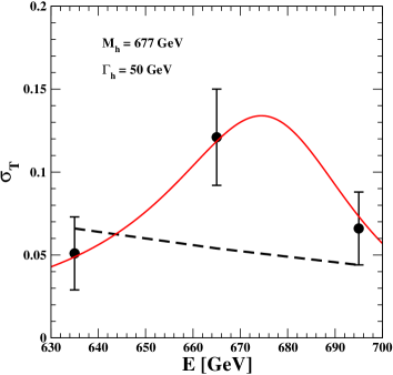
Figure 6: As in Fig.4 for $M_{h}=$ 677 GeV and $\Gamma_{h}=$ 50 GeV. Fitted parameters are $\sigma_{R}=0.131\pm 0.036$ fb and $\sigma_{B}=0.002^{+0.012}_{-0.002}$ fb, or total fitted background $N^{\rm fit}_{B}=1^{+5}_{-1}$. Errors from fit give $\chi^{2}=$ 2.41 with $\chi^{2}_{\rm min}=0.1$. The dashed line is ATLAS background estimate.

Conclusion: with Eq.(44) and the average background as free parameter, one finds an excellent fit of the ATLAS data, see Fig.4, with our reference $\Gamma_{h}/M_{h}$ ratio, a $\sigma_{R}$ as in Table 1 and a small background. Acceptable fits can however be obtained with smaller widths and a background closer to ATLAS value, see Fig.5. Altogether, the observed range of the various parameters can be approximated as: $M_{h}\sim(680\pm 10)$ GeV, $\Gamma_{h}\sim(32\pm 18)$ GeV, $\sigma_{R}\sim(0.15\pm 0.05)$ fb, $\sigma_{B}\sim 0.01^{+0.03}_{-0.01}$ fb. In particular, the fitted $M_{h}$ stays in the theoretical band $M_{h}=690\pm 10~{}({\rm stat})\pm 20~{}({\rm sys})$ GeV obtained when our lattice data [8] are combined with the leading-order $m_{h}-\langle\Phi\rangle$ relation.

Therefore, for the special role of the 4-lepton channel, further checks of the background and further statistical tests are needed. For instance, with the 36.1 fb^-1 luminosity, the deep diving of the local $p_{0}$ at the 3.6 sigma level [43] was already suggesting a new narrow resonance at 700 GeV. It remains to be seen if an unambiguous answer could still be obtained with the present LHC configuration or must be postponed to the high-luminosity phase .

7. Summary and outlook

After the observation of the narrow scalar resonance at 125 GeV, Veltman’s original idea of a naturally large Higgs particle mass seems to be ruled out. Yet, perhaps, the last word has not been said. If SSB in $\Phi^{4}$ theories is really a weak first-order phase transition, as indicated by most recent lattice simulations, one should consider approximations to the effective potential which are consistent with this scenario. Then, by combining analytic calculations and lattice simulations, it becomes conceivable that, besides the known resonance with mass $m_{h}\sim$ 125 GeV, a new excitation with mass $M_{h}\sim 700$ GeV might show up. The peculiarity, though, is that the heavier state should couple to longitudinal vector bosons with the same typical strength of the low-mass state and would thus represent a relatively narrow resonance. In this case, such hypothetical new resonance would naturally fit with some excess of 4-lepton events observed by ATLAS around 680 GeV. Analogous data from CMS are needed to definitely confirm or disprove this interpretation.

But, before concluding, I will discuss the possible implications that a two-mass structure of the Higgs field may have for radiative corrections. Our lattice simulations in Sect.4 indicate two regimes of the inverse propagator $G^{-1}(p)$. This behaves as $(p^{2}+m^{2}_{h})$ in the low-$p^{2}$ limit, see Fig.3 for $p^{2}<$ 0.1, and as $(p^{2}+M^{2}_{h})$ at larger $p^{2}$, see Fig.2 for $p^{2}>$ 0.1. Extrapolating the observed scaling $M^{2}_{h}\sim m^{2}_{h}\ln(\Lambda_{s}/M_{h})$ to very large values of $\Lambda_{s}$ gives the idea, in Minkowski space, of two vastly different mass-shell regions, as when the spectral density has not the standard single-peak structure.

By expressing $G^{-1}(p)=p^{2}-\Pi(p)$, the observed $m_{h}-M_{h}$ difference confirms the point of view of the Introduction that, in the broken-symmetry phase, the self-energy function $\Pi(p)$ exhibits a non-trivial momentum dependence. This can be interpreted as the coexistence, in the cutoff theory, of two kinds of quasi-particles associated respectively with two distinct aspects of the effective potential: its quadratic shape and the zero-point energy which determines its depth. The analogy with superfluid He-4, where the observed energy spectrum arises by combining the two quasi-particle spectra of phonons and rotons, would then suggest a model propagator

$$G(p)=\frac{1-I(p)}{2}\frac{Z_{1}}{p^{2}+m^{2}_{h}}+\frac{1+I(p)}{2}\frac{Z_{2}}{p^{2}+M^{2}_{h}}$$ (45)

where the interpolating function $I(p)$ depends on an intermediate momentum scale $p_{0}$ and tends to $+1$ for large $p^{2}\gg p^{2}_{0}$ and to $-1$ when $p^{2}\to 0$. For instance, by fixing sharply the central values of Sect.4, $Z_{1}=$ 0.945, $m_{h}=$ 0.0769, $Z_{2}=$ 0.966, $M_{h}=$ 0.0933, the form $I(p)=\tanh(p^{2}-p^{2}_{0})/\gamma$ gives a good fit to the lattice data, $\chi^{2}=29/(40-6)$, for $p^{2}_{0}=0.087$ and $\gamma=0.0043$. But small changes of the $Z$’s and of the masses can induce sizeable changes of $p^{2}_{0}$ and $\gamma$ indicating that the crossover region may be wider than with a simple step function. Moreover, any trial form for $I(p)$ in Eq.(45) introduces a model dependence that could obscure the significance of the results. Thus, while the lattice data indicate that, in Minkowski space, the spectral density should exhibit a two-peak structure, in practice, performing the analytic continuation in a non-perturbative regime, and in a numerical simulation where only a discrete set of data is available, is a difficult task [44].

To get some intuitive insight on the interplay of the two masses in radiative corrections, I will thus refer to a work of van der Bij [18] where a propagator which resembles Eq.(45) was also considered. To this end, he starts from two observations. First, renormalizability, by itself, does not mean a single-particle peak but only a spectral density which falls off sufficiently fast at infinity. Second, the Higgs field fixes the vacuum state of the theory which determines the masses of all other particles. Therefore, the Higgs field itself remains different and it is not unreasonable to expect a spectral density which is not a single $\delta-$function. Here, he does not mention the two-branch spectrum of superfluid He-4 but the idea of the SSB vacuum as some kind of medium seems implicit in this remark. With a definite example [45], he then considers the possibility that the physical Higgs boson is actually a mixture of two states with a spectral density approximated by two $\delta-$function peaks. The resulting propagator structure can be written as ($-1\leq\eta\leq 1$)

$$G(p)\sim\frac{1-\eta}{2}\frac{1}{p^{2}+m^{2}_{h}}+\frac{1+\eta}{2}\frac{1}{p^{2}+M^{2}_{h}}$$ (46)

and could be used in the analysis of the $\rho-$parameter [46, 47]. Since the two-loop correction [48] is completely negligible for masses below 1 TeV, one can restrict to the one-loop level, where the two branches Eq.(46) do not mix, as when replacing in the main logarithmic term an effective mass $m_{\rm eff}\sim\sqrt{m_{h}M_{h}}~{}(M_{h}/m_{h})^{\eta/2}$. In our case, this would be between $m_{h}=$ 125 GeV and $M_{h}\sim$ 700 GeV so that it becomes important to understand how well the mass parameter obtained indirectly from radiative corrections agrees with the $m_{h}=$ 125 GeV, measured directly at LHC.

Here, after the (partial) reassessment of the NuTeV anomaly [49, 50], only two measurements give sharp indications. Namely, $A_{\rm FB}(b)$ which favors a large effective mass and $A_{\rm LR}$ from SLD which goes in the opposite direction. This is well illustrated in the PDG review [19]. In fact, from the experimental set ($A_{\rm LR}$, $M_{Z}$, $\Gamma_{Z}$, $m_{t}$), one would predict the pair $[m_{\rm eff}=38^{+30}_{-21}$ GeV, $\alpha_{s}(M_{z})=0.1182(47)$]. While, from the set ($A_{\rm FB}(b,c)$, $M_{Z}$, $\Gamma_{Z}$, $m_{t}$), the other pair [$m_{\rm eff}=348^{+187}_{-124}$ GeV, $\alpha_{s}(M_{z})=0.1278(50)$].

These two extreme cases show that, at this level of precision, we should try to evaluate the uncertainty induced by strong interactions. This enters indirectly, for instance in the $M_{w}-M_{z}$ interdependence, through the contribution of the hadronic vacuum polarization to $\Delta\alpha(M_{z})$, but also directly through the value of $\alpha_{s}(M_{z})$. More precisely, in the two examples considered above, this uncertainty enters through $r(M_{z})$, the strong-interaction correction to the quark-parton model in $\sigma(e+e^{-}\to hadrons)$ at center of mass energy $Q=M_{z}$. Through the total W and Z widths, and the LEP1 peak cross sections, this affects all quantities, even the pure leptonic widths and asymmetries.

Since a small coupling does not guarantee, by itself, a good convergence of the perturbative expansion, one should seriously consider that, even at large center of mass energies, the experimental quantity $r^{\rm EXP}(Q)$ obtained from the data can sizeably differ from its theoretical prediction $r^{\rm TH}(Q)=1+\alpha_{s}(Q)/\pi+...$ computed from the first few terms. In this case, for a real precision test, instead of treating $\alpha_{s}(M_{z})$ as a free parameter, one could extrapolate $r^{\rm EXP}(Q)$ toward $Q=M_{z}$ and use this value to extract the EW corrections from experiments.

As pointed out in ref.[51], in fact, there is some excess in the data so that, to extrapolate correctly from PETRA, PEP and TRISTAN toward the $Z$ peak, one should replace in $r^{\rm TH}$ (34 GeV) a considerably larger $\alpha_{s}$(34 GeV)$\sim$ 0.17 instead of the canonical 0.14 predicted from deep inelastic scattering. This $\Delta\alpha_{s}=+0.03$ is a small $+1\%$ effect in the QCD correction but is visible in the slope of the $\gamma-Z$ interference. On the $Z$ peak, the effect is smaller because we are now speaking of a shift from $\alpha_{s}(M_{z})=0.118$ to $\alpha_{s}(M_{z})=0.128$ which is just a $+0.3\%$ effect in $r^{\rm TH}(M_{z})$. Nevertheless, the Higgs mass parameter extracted from the LEP1 data would be considerably increased [52, 53].

Later on, some excess in the total hadronic cross section had also been observed at LEP2 [54, 55, 56] so that the whole issue of $\sigma(e+e^{-}\to hadrons)$ was reconsidered by Schmitt [57] in a thorough analysis of all data in the range 20 GeV$\leq Q\leq$ 209 GeV. His conclusion was that, individually, none of the measurements shows a significant discrepancy. However, when taken together, there is an overall excess at the 4-sigma level. If translated into the QCD correction, this corresponds to replacing the higher range of values $\alpha_{s}(M_{z})\gtrsim$ 0.128 in $r^{\rm TH}(M_{z})$ and, if used to evaluate the EW corrections, would increase the value of $m_{\rm eff}$ obtained from many experimental quantities. For instance, from the set ($A_{\rm LR}$, $A_{\rm FB}(b,c)$, $M_{Z}$, $\Gamma_{Z}$, $m_{t}$).

In this sense, the present view, that the Higgs mass parameter extracted indirectly from radiative corrections agrees perfectly with the $m_{h}=$ 125 GeV measured directly at LHC, is not free of ambiguities and one could in the end discover other motivations for a new resonance, quite independently of the effective potential and/or of lattice simulations of the propagator. This emphasizes once more the importance of new, combined LHC measurements, starting from the “golden” 4-lepton channel around 700 GeV.

DEDICATION

This paper is dedicated to the memory of Professor M. J. G. Veltman. Perhaps now, that he is no longer with us, we can better realize how much his moral legacy has transcended the purely scientific.

References

- [1] M. Veltman, Acta Phys. Polon. B8 (1977) 475.
- [2] F. Englert, R. Brout, Phys. Rev. Lett. 13 (1964) 321.
- [3] P.W. Higgs, Phys. Lett. 12 (1964) 132.
- [4] S. L. Glashow, Nucl. Phys. B22 (1961) 579.
- [5] ATLAS Collaboration (G. Aad et al.), Phys. Lett. B716 (2012) 1.
- [6] CMS Collaboration (S. Chatrchyan et al.), Phys. Lett. B 716 (2012) 30.
- [7] S.R. Coleman, E.J. Weinberg, Phys. Rev. D7 (1973) 1888.
- [8] M. Consoli, L. Cosmai, Int. J. Mod. Phys. A 35 (2020) 2050103, hep-ph/2006.15378.
- [9] M. Consoli, L. Cosmai, Symmetry 12, 2020, 2037; doi:10.3390/sym12122037.
- [10] P.H. Lundow, K. Markström, Physical Review E 80 (2009) 031104.
- [11] P.H. Lundow, K. Markström, Nucl. Phys. B845 (2011) 120.
- [12] S. Akiyama, et al., Phys. Rev. D 100 (2019) 054510.
- [13] P.Cea, M.Consoli, L.Cosmai, Nucl.Phys.Proc.Suppl. 129 (2004)780, hep-lat/0309050.
- [14] P. Cea, L. Cosmai, ISRN High Energy Phys. (2012) 637950, hep-ph/0911.5220.
- [15] M. Consoli, P.M. Stevenson, Z. Phys. C 63 (1994) 427, hep-ph/9310338.
- [16] M. Consoli, P.M. Stevenson, Phys. Lett. B 391 (1997) 144.
- [17] M. Consoli, P.M. Stevenson, Int. J. Mod. Phys. A 15(2000) 133, hep-ph/9905427.
- [18] J. J. van der Bij, Acta Phys. Polon. B11 (2018) 397.
- [19] M. Tanabashi et al. (Particle Data Group), Phys. Rev. D 98 (2018) 030001.
- [20] D. Shirkov, Lectures at KEK, April 1991, KEK-91-13, 1992 (unpublished).
- [21] K. G. Chetyrkin, S. G. Gorishny, S. A. Larin, and F. V. Tkachov, Phys. Lett. B 132(1983) 351.
- [22] D. I. Kazakov, Phys. Lett. B 133 (1983) 406.
- [23] P. M. Stevenson, Z. Phys. C35 (1987) 467.
- [24] M. Consoli and P. M. Stevenson, Mod. Phys. Lett. A 11 (1996) 2511.
- [25] T. Barnes and G. I. Ghandour, Phys. Rev. D22 (1980) 924.
- [26] P. M. Stevenson, Phys. Rev. D32 (1985) 1389.
- [27] I. Stancu and P. M. Stevenson, Phys. Rev. D42 (1990) 2710.
- [28] P. Cea and L. Tedesco, Phys. Rev. D55 (1997) 4967.
- [29] P. M. Stevenson, Nucl. Phys. B729 (2005) 542.
- [30] P. Cea, M. Consoli, L. Cosmai and P. M. Stevenson, Mod. Phys. Lett. A14 (1999) 1673.
- [31] P. Castorina, M. Consoli, D. Zappalà, J. Phys. G 35 (2008) 075010, hep-ph/0710.0458.
- [32] M. J. G. Veltman and F. Yndurain, Nucl. Phys. B 325 (1989) 1.
- [33] B. W. Lee, C. Quigg, H. B. Tacker, Phys. Rev. D 16 (1977) 1519.
- [34] J.M. Cornwall, D.N. Levin, G. Tiktopoulos, Phys. Rev. D 10 (1974) 1145.
- [35] M.S. Chanowitz, M.K. Gaillard, Nucl. Phys. B 261 (1985) 379.
- [36] J. Bagger and C. Schmidt, Phys. Rev. D 41 (1990) 264.
- [37] M. Consoli and L. Cosmai, arXiv:2007.10837v2 [hep-ph], 25/12/2020.
- [38] M. Aaboud et al. (ATLAS), Eur. Phys. J. C 78 (2018) 293, arXiv:hep-ex/1712.06386.
- [39] G. Aad et al. (ATLAS), Eur. Phys. J. C 81 (2021) 332, arXiv:2009.14791[hep-ex],
- [40] A. Djouadi, Phys. Rept. 457 (2008) 1, arXiv:hep-ph/0503172.
- [41] Report of the LHC Higgs Cross Section Working Group, S. Dittmaier et al., Eds.,arXiv:1101.0593 [hep-ph].
- [42] G. L. Kane, W. W. Repko, W. B. Rolnick, Phys. Lett. B 148 (1984) 367.
- [43] D. Denysiuk, PhD Thesis 2017, https://tel.archives-ouvertes.fr/tel-01681802v2.
- [44] D. Dudal, O. Oliveira, M. Roelfs, P. Silva, Nucl. Phys. B 952, 114912 (2020).
- [45] A. Hill and J.J. van der Bij, Phys. Rev. D36 (1987) 3463.
- [46] D. A. Ross and M. J. G. Veltman, Nucl. Phys. B 95, 135 (1975).
- [47] M. J. G. Veltman, Nucl. Phys. B 123, 89 (1977).
- [48] J. J. van der Bij and M. Veltman, Nucl. Phys. B 231 (1984) 205.
- [49] W. Bentz, I.C. Cloët, J.T. Londergan, A.W. Thomas, Phys. Lett. B 693 (2010) 462.
- [50] P. Coloma, P. B. Denton, M.C. Gonzalez-Garcia, M. Maltoni, T. Schwetzg, JHEP 04, 116 (2017).
- [51] V. Branchina, M. Consoli, R. Fiore and D. Zappalà, Phys. Rev. D46 (1992) 75.
- [52] M. Consoli and Z. Hioki, Mod. Phys. Lett. A10 (1995) 845.
- [53] M. Consoli and Z. Hioki, Mod. Phys. Lett. A10 (1995) 2245.
- [54] J. Erler, arXiv:hep-ph/0310202, 16/10/2003.
- [55] G. Wilkinson, arXiv:hep-ex/0205103, 30/05/2002.
- [56] S. Wynhoff, arXiv:hep-ex/0101016, 12/01/2001.
- [57] M. Schmitt, arXiv:hep-ex/0401034v2, 25/01/2004.