Singular Behavior of the Macroscopic Quantity Near the Boundary for a Lorentz-Gas Model with the Infinite-Range Potential

Abstract

Possibility of the diverging gradient of the macroscopic quantity near the boundary is investigated by a mono-speed Lorentz-gas model, with a special attention to the regularizing effect of the grazing collision for the infinite-range potential on the velocity distribution function (VDF) and its influence on the macroscopic quantity. By careful numerical analyses of the steady one-dimensional boundary-value problem, it is confirmed that the grazing collision suppresses the occurrence of a jump discontinuity of the VDF on the boundary. However, as the price for that regularization, the collision integral becomes no longer finite in the direction of the molecular velocity parallel to the boundary. Consequently, the gradient of the macroscopic quantity diverges, even stronger than the case of the finite-range potential. A conjecture about the diverging rate in approaching the boundary is made as well for a wide range of the infinite-range potentials, accompanied by the numerical evidence.

1 Introduction

It has been known for a long time that the velocity distribution function (VDF) of molecules in a rarefied gas has a jump discontinuity, in general, on the boundary in the direction of molecular velocity parallel to the boundary, e.g. see Refs. K69 ; S07 . Originating from this feature, the macroscopic quantities defined as the moment of VDF change steeply near the boundary in the direction normal to it. Here, the steep change does not mean the Knudsen layer (the kinetic boundary layer) in slightly rarefied gases, but rather means the singular behavior of those quantities at the bottom of the ballistic non-equilibrium region with the thickness of the mean-free-path of a molecule. The Knudsen layer is just an example of such a non-equilibrium region. Note that the non-equilibrium region extends much wider and possibly even to the entire region in low pressure circumstances or in micro-scale physical systems. The variation becomes steeper indefinitely in approaching the boundary, and the variation rate diverges finally on the boundary. The diverging rate follows a universality such that it depends on the local geometry of the boundary. The detailed discussions can be found in Ref. TT17 .

In the literature TF13 ; CLT14 ; TT17 ; TST19 ; CH15 , the diverging rate has been discussed in the connection with a jump discontinuity of the VDF both qualitatively and quantitatively. However, in those discussions it is supposed that the collision integral can be split into the gain and the loss term, namely the case where the collision frequency is finite. This means that the investigated molecular models are the finite-range potentials or the cutoff potentials if the infinite-range potentials are in mind C88 ; S07 . The grazing collisions that change the molecular trajectory only slightly have been studied intensively for the infinite range potentials as an attractive mathematical topics in the last two decades, e.g., Refs. D95 ; DG00 ; V02 ; AV02 ; MS07 ; AMUXY10 ; AMUXY11 ; GS11 ; CH11 ; JL19 , and are found to have a regularizing effect on the VDF for such potentials.

In view of those mathematical studies, it is expected that the jump discontinuity of the VDF is not allowed even on the boundary for the infinite-range potential, which may, in turn, suppress the diverging gradient of macroscopic quantities because of the absence of its origin. It motivates us to study whether or not the diverging gradient occurs for the infinite range potentials by using a mono-speed Lorentz-gas model equation. This model equation, in place of the original Boltzmann equation, has already been used in Ref. T15 to investigate the propagation of the jump discontinuity in the initial data and has been shown to capture the features of the propagation well. In this sense, the present work may also be regarded as an extension of Ref. T15 to the steady one-dimensional boundary-value problem. As will be clarified later, the grazing collisions for the infinite range potential indeed do not allow the jump discontinuity of the VDF on the boundary. Nevertheless, as the price for this regularizing effect, the collision integral no longer remains finite; consequently, the diverging gradient manifests itself more strongly than the case of the finite range potential when approaching the boundary.

The paper is organized as follows. First, the mono-speed Lorentz-gas model is introduced and the one-dimensional boundary-value problem is set up in Sec. 2.Thus, the singularity near the flat boundary will be investigated. Then, in Sec. 3, two numerical methods are introduced. One is a rather direct approach that is particularly suitable for the study of the finite-range and the cutoff potential and is briefly explained in Sec. 3.1. The other is the approach based on the Galerkin method, applicable to the infinite-range potential as well, and explained in detail in Sec. 3.2. The numerical results are presented in Sec. 4. The results for the cutoff potential with various cutoff sizes and those for the corresponding infinite-range potential are compared in the Maxwell-molecule-type case. Furthermore, the diverging rate of the gradient of the macroscopic quantity are identified for the same case in Sec. 4.2. A conjecture on the diverging rate for other infinite range potentials is made in Sec. 4.3, accompanied by the additional numerical evidence. The paper is concluded in Sec. 5.

2 Lorentz-Gas Model

We consider the following mono-speed Lorentz-gas model that is two-dimensional both in the position and the molecular velocity space in the present paper.

$$\frac{\partial f}{\partial t}+\alpha_{i}\frac{\partial f}{\partial x_{i}} =\int_{|\bm{\beta}|=1}b(|\bm{\alpha}\cdot\bm{\beta}|)\{f(t,\bm{x},\bm{\alpha}_{*})-f(t,\bm{x},\bm{\alpha})\}d\bm{\beta},$$ (1a)

$$\bm{\alpha}_{*} =\bm{\alpha}-2(\bm{\beta\cdot\bm{\alpha}})\bm{\beta}.$$ (1b)

The same model was used in Ref. T15 for the study of the grazing collision effects on the time evolution from the initial data with a jump discontinuity. Here, $f$ is the dimensionless velocity distribution function (VDF), $t$ is the dimensionless time, $\bm{x}$ is the dimensionless position vector, and $\bm{\alpha}$, $\bm{\alpha_{*}}$, and $\bm{\beta}$ are unit vectors, where the reference scales of quantities are chosen in such a way that both of the Strouhal and the Knudsen number are unity. The unit vectors $\bm{\alpha}$ and $\bm{\alpha_{*}}$ represent the dimensionless velocity of a molecule, the size of which does not change by the present collision integral, i.e., the right-hand side. The molecular velocity changes only its direction by the effect of the right-hand side. The direction of change is represented by another unit vector $\bm{\beta}$. The function $b$ represents the interaction effect and is non-negative. Here, it is assumed to take the following form in order to mimic the hard-disk and the inverse-power-law potential model:

$$b(|\bm{\alpha}\cdot\bm{\beta}|) =B_{\gamma+2}^{-1}|\bm{\alpha}\cdot\bm{\beta}|^{\gamma},\quad(-3<\gamma\leq 1),$$ (2a)

$$B_{\mathrm{\gamma}} =\int_{|\bm{\beta}|=1}|\bm{\alpha}\cdot\bm{\beta}|^{\gamma}d\bm{\beta}.$$ (2b)

As explained in Ref. T15 , the setting $\gamma=1$ is the hard-disk potential, while the setting $\gamma=-\frac{n+1}{n-1}$ well mimics the angular singularity (or the grazing collision effect) occurring in the Boltzmann equation for the $(n-1)$-th inverse-power-law potential, where $n=5$ (or $\gamma=-3/2$) corresponds to the celebrated Maxwell molecule. It should be noted that $B_{\gamma}$ is the (dimensionless) collision frequency for the adopted interaction potential and remains finite as far as $\gamma>-1$. The range $-1<\gamma<1$ is not covered by the inverse-power-law potential and the collision integral can be split into the so-called gain and loss term safely; this range of $\gamma$ will be referred to the finite-range potential in the present paper. For $-3<\gamma\leq-1$ (or $n>2$), $B_{\gamma}$ is no longer finite but diverges and the collision term can be treated only when the collision integral is treated as a whole; this range of $\gamma$ will be referred to the infinite-range potential in the present paper. The setting $\gamma=-3$ (or $n=2$) corresponds to the Coulomb potential and the collision term no longer remains finite. The factor $B_{\gamma+2}$ occurring in (2a) is the effective collision frequency based on the momentum change in collisions. As is seen from (2b), it does not diverge for $\gamma>-3$.

2.1 Problem and Formulation

In order to study the possibility of the diverging gradient of macroscopic quantities, the following steady one-dimensional boundary-value problem is considered for the above Lorentz-gas model (1):

$$\alpha_{1}\frac{\partial f}{\partial x_{1}} =\int_{|\bm{\beta}|=1}b(|\bm{\alpha}\cdot\bm{\beta}|)\{f(x_{1},\bm{\alpha}_{*})-f(x_{1},\bm{\alpha})\}d\bm{\beta},$$ (3a)

$$\mbox{b.c. }f =\frac{1}{2\pi}(1\pm c),\quad x_{1}=\mp\frac{1}{2},\ \alpha_{1}\gtrless 0,$$ (3b)

where $0<c<1$ is a constant. The (dimensionless) density $\rho$ is expressed as the following moment of $f$:

$$\rho=\int_{|\bm{\alpha}|=1}fd\bm{\alpha},$$ (4)

the behavior of which near the boundary $x_{1}=-1/2$ is the primary target of the present study.

By noting the relation

$$|\bm{\alpha}\cdot\bm{\beta}|=\Big{(}\frac{1-\bm{\alpha}\cdot\bm{\alpha}_{*}}{2}\Big{)}^{1/2},$$ (5)

the above problem (3) is reduced to that for $g\equiv(2\pi f-1)/c$:

$$\sin\theta\frac{\partial g}{\partial x_{1}} =C_{\gamma}[g],$$ (6a)

$$g =\pm 1,\quad x_{1}=\mp\frac{1}{2},\ \sin\theta\gtrless 0.$$ (6b)

Here

$$C_{\gamma}[g] =\frac{1}{B_{\gamma+2}}\int_{-\pi}^{\pi}\Big{(}\frac{1-\cos\theta_{*}}{2}\Big{)}^{\gamma/2}\{g(x_{1},\theta+\theta_{*})-g(x_{1},\theta)\}d\theta_{*}$$

$$=\frac{1}{B_{\gamma+2}}\int_{-\pi}^{\pi}|\sin\frac{\phi-\theta}{2}|^{\gamma}\{g(x_{1},\phi)-g(x_{1},\theta)\}d\phi,$$ (7)

$$B_{\gamma} \equiv\int_{|\bm{\beta}|=1}|\bm{\alpha}\cdot\bm{\beta}|^{\gamma}d\bm{\beta}=\int_{-\pi}^{\pi}|\cos\varphi|^{\gamma}d\varphi=2\int_{0}^{\pi}|\sin\frac{\phi}{2}|^{\gamma}d\phi,$$ (8)

and $\theta$ and $\theta+\theta_{*}$ respectively indicate the clockwise angle of the unit vectors $\bm{\alpha}$ and $\bm{\alpha}_{*}$ measured from the $x_{2}$-direction. Note that in (7), the range of integration for $\phi$ is shifted by $\theta$ because of the $2\pi$-periodicity. The density is then reduced to the following moment of $g$:

$$\rho(x_{1})=1+\frac{c}{2\pi}\int_{-\pi}^{\pi}g(x_{1},\theta)d\theta\equiv 1+c\rho_{g}(x_{1}).$$ (9)

2.2 Angular Cutoff

When $-1<\gamma$, the $C_{\gamma}$ defined in (7) can be treated separately as:

$$C_{\gamma}[g] =C_{\gamma}^{+}[g]-\nu_{\gamma}g,$$ (10a)

$$C_{\gamma}^{+}[g] =\int_{-\pi}^{\pi}b_{\gamma}(\phi-\theta)g(x_{1},\phi)d\phi,$$ (10b)

$$\nu_{\gamma} =\int_{-\pi}^{\pi}b_{\gamma}(\phi-\theta)d\phi=\int_{-\pi}^{\pi}b_{\gamma}(\phi)d\phi,$$ (10c)

$$b_{\gamma}(\varphi)\equiv\frac{1}{B_{\gamma+2}}|\sin\frac{\varphi}{2}|^{\gamma}.$$ (10d)

It is not the case, however, when $-3<\gamma\leq-1$, since $b_{\gamma}(\varphi)$ is singular for $\varphi\to 0$ strongly enough for the integrability not to be assured. Physically, it implies that the grazing events that are little effective to change the particle velocity are all counted as the collision. Hence in the literature, the truncation of the range of $\varphi$, the so-called angular cutoff C88 , is introduced in order to avoid counting such an enormous amount of grazing events. The infinite-range potential with the cutoff will be simply called the cutoff potential in what follows. With the size of the cutoff $\epsilon$, the following notations for the cutoff potential are introduced here:

$$C_{\gamma,\epsilon}[g] =C_{\gamma,\epsilon}^{+}[g]-\nu_{\gamma,\epsilon}g,$$ (11a)

$$C_{\gamma,\epsilon}^{+}[g] =\int_{-\pi}^{\pi}b_{\gamma,\epsilon}(\phi-\theta)g(x_{1},\phi)d\phi,$$ (11b)

$$\nu_{\gamma,\epsilon} =\int_{-\pi}^{\pi}b_{\gamma,\epsilon}(\phi-\theta)d\phi=\int_{-\pi}^{\pi}b_{\gamma,\epsilon}(\phi)d\phi,$$ (11c)

where

$$b_{\gamma,\epsilon}(\varphi) =\begin{cases}\frac{B_{\gamma+2}}{B_{\gamma+2,\epsilon}}b_{\gamma}(\varphi),&\epsilon<\varphi<2\pi-\epsilon\\ 0,&\mathrm{otherwise}\end{cases},\quad(0<\varphi<2\pi),$$ (12)

$$B_{\gamma,\epsilon} =2\int_{\epsilon}^{\pi}|\sin\frac{\phi}{2}|^{\gamma}d\phi,$$ (13)

and the factor $B_{\gamma+2}/B_{\gamma+2,\epsilon}$ is used so that the effective collision cross-section based on the momentum change B94 ; T15 becomes common between the cutoff and the infinite-range potential for the same $\gamma$.

2.3 Small Reduction Using Problem Symmetry

The $g$ having the following symmetry matches the boundary-value problem (6):

$$g(\cdot,\theta) =g(\cdot,\pi-\theta),\quad(\frac{\pi}{2}<\theta<\pi),$$ (14a)

$$g(\cdot,\theta) =g(\cdot,-\pi-\theta),\quad(-\pi<\theta<-\frac{\pi}{2}),$$ (14b)

$$g(x_{1},\theta) =-g(-x_{1},-\theta),\quad(0<x_{1}<\frac{1}{2},\ -\frac{\pi}{2}<\theta<\frac{\pi}{2}).$$ (14c)

The properties (14a) and (14b) admit the following expression of $\rho_{g}$

$$\rho_{g}(x_{1})=\frac{1}{\pi}\int_{-\pi/2}^{\pi/2}g(x_{1},\theta)d\theta,$$ (15)

and the following transformation of $C_{\gamma}$:

$$C_{\gamma}[g] =\int_{-\pi}^{\pi}b_{\gamma}(\phi-\theta)\{g(x_{1},\phi)-g(x_{1},\theta)\}d\phi$$

$$=\int_{-\pi/2}^{\pi/2}b_{\gamma}(\phi-\theta)\{g(x_{1},\phi)-g(x_{1},\theta)\}d\phi$$

$$+\int_{-\pi}^{-\pi/2}b_{\gamma}(\phi-\theta)\{g(x_{1},\phi)-g(x_{1},\theta)\}d\phi$$

$$+\int_{\pi/2}^{\pi}b_{\gamma}(\phi-\theta)\{g(x_{1},\phi)-g(x_{1},\theta)\}d\phi$$

$$=\int_{-\pi/2}^{\pi/2}b_{\gamma}(\phi-\theta)\{g(x_{1},\phi)-g(x_{1},\theta)\}d\phi$$

$$+\int_{-\pi}^{-\pi/2}b_{\gamma}(\phi-\theta)\{g(x_{1},-\pi-\phi)-g(x_{1},\theta)\}d\phi$$

$$+\int_{\pi/2}^{\pi}b_{\gamma}(\phi-\theta)\{g(x_{1},\pi-\phi)-g(x_{1},\theta)\}d\phi$$

$$=\int_{-\pi/2}^{\pi/2}b_{\gamma}(\phi-\theta)\{g(x_{1},\phi)-g(x_{1},\theta)\}d\phi$$

$$+\int_{-\pi/2}^{0}b_{\gamma}(-\psi-\pi-\theta)\{g(x_{1},\psi)-g(x_{1},\theta)\}d\psi\quad(\psi=-\pi-\phi)$$

$$+\int_{0}^{\pi/2}b_{\gamma}(\pi-\psi-\theta)\{g(x_{1},\psi)-g(x_{1},\theta)\}d\psi\quad(\psi=\pi-\phi)$$

$$=\int_{-\pi/2}^{\pi/2}\{b_{\gamma}(\phi-\theta)+b_{\gamma}(\pi-\phi-\theta)\}\{g(x_{1},\phi)-g(x_{1},\theta)\}d\phi,$$ (16)

where the relation

$$b_{\gamma}(-\psi-\theta-\pi)=b_{\gamma}(\psi+\theta+\pi)=b_{\gamma}(\psi+\theta-\pi)=b_{\gamma}(\pi-\psi-\theta),$$ (17)

has been used. Moreover, by using (14c), the problem (6) is reduced to the following problem in $-1/2<x_{1}<0$ and $-\pi/2<\theta<\pi/2$:

$$\sin\theta\frac{\partial g}{\partial x_{1}} =C_{\gamma}[g],$$ (18a)

$$C_{\gamma}[g] =\int_{-\pi/2}^{\pi/2}\{b_{\gamma}(\phi-\theta)+b_{\gamma}(\pi-\phi-\theta)\}\{g(x_{1},\phi)-g(x_{1},\theta)\}d\phi,$$ (18b)

$$\mathrm{b.c.\ }\begin{cases}g(0,\theta)=-g(0,-\theta)&-\pi/2<\theta<0\\ g(-1/2,\theta)=1&0<\theta<\pi/2\end{cases}.$$ (18c)

Since $b_{\gamma,\epsilon}$ matches the same relation (17) as $b_{\gamma}$, the problem (18) is written for the corresponding cutoff potential by simply replacing $C_{\gamma}$ with $C_{\gamma,\epsilon}$:

$$\sin\theta\frac{\partial g}{\partial x_{1}} =C_{\gamma,\epsilon}[g],$$ (19a)

$$C_{\gamma,\epsilon}[g] =\int_{-\pi/2}^{\pi/2}\{b_{\gamma,\epsilon}(\phi-\theta)+b_{\gamma,\epsilon}(\pi-\phi-\theta)\}\{g(x_{1},\phi)-g(x_{1},\theta)\}d\phi,$$ (19b)

$$\mathrm{b.c.\ }\begin{cases}g(0,\theta)=-g(0,-\theta)&-\pi/2<\theta<0\\ g(-1/2,\theta)=1&0<\theta<\pi/2\end{cases}.$$ (19c)

Remind that $C_{\gamma}$ can be treated as

$$C_{\gamma}[g] =C_{\gamma}^{+}[g]-\nu_{\gamma}g,$$ (20a)

$$C_{\gamma}^{+}[g] =\int_{-\pi/2}^{\pi/2}\{b_{\gamma}(\phi-\theta)+b_{\gamma}(\pi-\phi-\theta)\}g(x_{1},\phi)d\phi,$$ (20b)

only when $-1<\gamma$. When $-3<\gamma\leq-1$, it is $C_{\gamma,\epsilon}$ which can be treated separately:

$$C_{\gamma,\epsilon}[g] =C_{\gamma,\epsilon}^{+}[g]-\nu_{\gamma,\epsilon}g,$$ (21a)

$$C_{\gamma,\epsilon}^{+}[g] =\int_{-\pi/2}^{\pi/2}\{b_{\gamma,\epsilon}(\phi-\theta)+b_{\gamma,\epsilon}(\pi-\phi-\theta)\}g(x_{1},\phi)d\phi.$$ (21b)

3 Methods of Numerical Analyses

In numerically treating the problem formulated in Sec. 2.3, the grid points in $\theta$-space are arranged to be symmetric with respect to $\theta=0$ in the region $-\pi/2\leq\theta\leq\pi/2$ so as to make $2N$ small intervals in both the positive and negative side:

$$0=\theta^{(0)}<\theta^{(1)}<\cdots<\theta^{(2N-1)}<\theta^{(2N)}=\frac{\pi}{2},\ \theta^{(-j)}=-\theta^{(j)},\ (j=1,\dots,2N).$$

Two different methods are prepared. One is the method making use of the numerical kernel SOA89 as in Ref. HT15 and is referred to as the direct method in the present paper. The direct method is able to treat (20) and (21) without numerical (or unphysical) oscillation, even when $g$ has a jump discontinuity at $\theta=0$ on the boundary; see Appendix A. This is the primary merit of the method and makes it suitable for the finite-range and the cutoff potential cases. As will be observed later through the results for the infinite-range potential, the jump discontinuity tends to vanish as $\epsilon\to 0$, but the collision integral instead tends to diverge at $\theta=0$ on the boundary, i.e., in the direction parallel to the boundary. This implies that a weaker formulation is unavoidable to study the infinite-range potential and motivates the approach using the Galerkin method.

Since the jump discontinuity is expected not to appear for the infinite-range potential, $g(x_{1},\theta)$ is approximated by the set of quadratic basis functions continuously. Then, the problem (18) is discretized by the projection into the space of the same basis functions in the Galerkin method. If the same is applied to the cutoff potential (19), artificial oscillations occur due to the jump discontinuity. However, as will be observed later in Sec. 4, it affects little to the behavior of $\rho_{g}$.

3.1 Direct Method for the Finite-Range and the Cutoff Potential

For the finite-range and the cutoff potential, the collision integral can be split into the loss and the gain term safely, and the problem is formally solved as :

$$g(x_{1},\theta) =\begin{cases}{\displaystyle e^{-\frac{\nu}{\sin\theta}(x_{1}+\frac{1}{2})}+\int_{-1/2}^{x_{1}}\frac{1}{\sin\theta}C^{+}[g]{(s,\theta)}e^{-\frac{\nu}{\sin\theta}(x_{1}-s)}ds,}\\ \qquad\qquad\qquad\qquad(0<\theta<\pi/2,\ -1/2<x_{1}<0),\\ {\displaystyle-g(0,-\theta)e^{-\frac{\nu}{\sin\theta}x_{1}}+\int_{0}^{x_{1}}\frac{1}{\sin\theta}C^{+}[g]{(s,\theta)}e^{-\frac{\nu}{\sin\theta}(x_{1}-s)}ds,}\\ \qquad\qquad\qquad\qquad(-\pi/2<\theta<0,\ -1/2<x_{1}<0),\end{cases}$$

where the subscript $\gamma$ and $\epsilon$ are omitted in $C^{+}$ and $\nu$, since there is no need of discrimination in the present context, while the arguments of $C^{+}[g]$ are indicated explicitly for clarity. The same omission convention will be applied in what follows, unless any confusions/ambiguities are expected. In the direct method, the solution $g$ is constructed by iteration from its initial guess. In this process, by substituting $g$ of the following approximation (the expansion in terms of the quadratic basis functions $\{Y_{j}(\theta)\}$, see Appendix A):

$$g(x_{1},\theta)=\sum_{j=-2N}^{2N}g_{j}(x_{1})Y_{j}(\theta),$$ (22)

with $g_{j\gtrless 0}$ being the value on the grid points in $\theta\gtrless 0$, the $C^{+}[g]$ at the grid point $\theta=\theta^{(i)}$ is expressed as $C^{+}[g]{(s,\theta^{(i)})}=\sum_{j=-2N}^{2N}g_{j}(s)C^{+}[Y_{j}]{(\theta^{(i)})}$. In this expression, the discrimination between $j=\pm 0$ is made when there is a jump discontinuity of $g$ at $\theta=0$. Although the analytical expression of $C^{+}[Y_{j}]$ in $\theta$ is obtained [see Appendix A, especially the descriptions below (50) there, for more details], $C^{+}[Y_{j}]{(\theta^{(i)})}$ at the grid point of $\theta$ are stored beforehand as the numerical kernel SOA89 in order to avoid repeating the same computation in the iteration in solving $g$. The integration with respect to $s$ is performed analytically after the quadratic interpolation of the data $C^{+}[g]{(s,\theta)}$ at the discrete position in $s$.

3.2 Galerkin Method

In the Galerkin method KR19 , irrespective of whether or not $g$ has a jump discontinuity in $\theta$, the approximate expression (22) of $g$ in terms of the quadratic basis functions $\{Y_{j}(\theta)\}$ is used as it stands, i.e., without the discrimination between $j=\pm 0$. More precisely, even for the finite-range and the cutoff potential, where $g$ is expected to have a jump discontinuity, (22) with $g_{0}=g_{-0}$ will be used in the solution process (see Appendix A). Before going into details, it should be noted that, thanks to the symmetric arrangement of the grid points $\theta^{(j)}$, it holds that $Y_{j}(\theta)=Y_{-j}(-\theta)$ and that $g_{j}(x_{1})=-g_{-j}(-x_{1})$ from the property (14c).

In order to construct the numerical procedure by the Galerkin method, first substitute (22) into (18a) with (18b) and then integrate the result multiplied with $Y_{i}(\theta)\ (i=-2N,\dots,2N)$ with respect to $\theta$. The result is that

$$\sum_{j=-2N}^{2N}A_{i,j}\frac{dg_{j}}{dx_{1}} =\sum_{j=-2N}^{2N}D_{i,j}g_{j},$$ (23)

$$A_{i,j} =\int_{-\pi/2}^{\pi/2}Y_{i}(\theta)Y_{j}(\theta)\sin\theta\ d\theta,$$

$$D_{i,j} =\int_{-\pi/2}^{\pi/2}Y_{i}(\theta)C[Y_{j}]{(\theta)}d\theta.$$

Here again the subscripts $\gamma$ and $\epsilon$ to $C$ are omitted. Note that the integration in the definitions of $A_{i,j}$ and $D_{i,j}$ can be done analytically and that

$$A_{i,j}=A_{j,i}=-A_{-i,-j},\quad(i,j=0,\pm 1,\dots,\pm 2N),$$ (24a)

$$A_{-i,j}=A_{i,-j}=0,\quad(i,j=1,\dots,2N),$$ (24b)

by definition. Moreover, $D_{i,j}=D_{j,i}$ holds, since $C$ is self-adjoint. In order to solve (23), it is relevant to check whether or not the following $(4N+1)\times(4N+1)$-symmetric matrix $A$ is regular:

$$A\equiv[A_{i,j}]= \left[\begin{array}[]{ccccccc}A_{-2N,-2N}&\cdots&A_{-2N,-1}&A_{-2N,0}&A_{-2N,1}&\cdots&A_{-2N,2N}\\ \vdots&\ddots&\vdots&\vdots&\vdots&\ddots&\vdots\\ A_{-1,-2N}&\cdots&A_{-1,-1}&A_{-1,0}&A_{-1,1}&\cdots&A_{-1,2N}\\ A_{0,-2N}&\cdots&A_{0,-1}&A_{0,0}&A_{0,1}&\cdots&A_{0,2N}\\ A_{1,-2N}&\cdots&A_{1,-1}&A_{1,0}&A_{1,1}&\cdots&A_{1,2N}\\ \vdots&\ddots&\vdots&\vdots&\vdots&\ddots&\vdots\\ A_{2N,-2N}&\cdots&A_{2N,-1}&A_{2N,0}&A_{2N,1}&\cdots&A_{2N,2N}\end{array}\right].$$

By direct calculations, it was observed that $A$ is not full rank and is rank deficient by one when $N=1,2,3$. This strongly suggests that the rank deficiency is due to the factor $\sin\theta$ in front of the spatial derivative of $g$ in (18a) is zero and the differential equation degenerates at $\theta=0$; thus the same rank deficiency is expected for other integer $N$. In what follows, the numerical procedure is constructed by supposing $\mathrm{rank}A=4N$, i.e., the rank deficiency by one.

Thanks to the property (24), the matrix $A$ is expressed as

$$A=[A_{i,j}]= \begin{array}[]{c}\left[\begin{array}[]{c|c}A^{(-)}&0\\ \hline\cr 0&A^{(+)}\end{array}\right]\begin{array}[]{c}(i<0)\\ (i>0)\end{array}\end{array},$$ (30)

$$\begin{array}[]{cc}(j<0),(j>0)\end{array}$$ (32)

where    indicates the row $i=0$, $\Big{|}$ indicates the column $j=0$, and $A^{(+)}$ and $A^{(-)}$ are $2N\times 2N$ symmetric matrices. The row $i=0$ and the column $j=0$ vector are non-zero. From (24), it is clear that $A_{0,0}=0$ and that $A_{i,j}^{(+)}=-A_{-i,-j}^{(-)}$, implying that both $A^{(+)}$ and $A^{(-)}$ are regular under the assumption $\mathrm{rank}A=4N$. Consequently, it follows that the $j>0$ part of the row $i=0$ of $A$ is expressed by the linear combination of the row vectors of $A^{(+)}$, while the $j<0$ part of the same row is expressed by the linear combination of the row vectors of $A^{(-)}$. That is, there are two sets of constants $\{c_{1},\dots c_{2N}\}$ and $\{\tilde{c}_{1},\dots\tilde{c}_{2N}\}$ such that

$$A_{0,j} =\sum_{i=1}^{2N}c_{i}A_{i,j}^{(+)},\quad(j>0),$$

$$A_{0,-j} =\sum_{i=1}^{2N}\tilde{c}_{i}A_{-i,-j}^{(-)}=-\sum_{i=1}^{2N}\tilde{c}_{i}A_{i,j}^{(+)},\quad(j>0).$$

Since $A_{0,-j}=-A_{0,j}$ by (24), it follows that $c_{i}=\tilde{c}_{i}$ and that

$$c_{i}=\sum_{j=1}^{2N}A_{0,j}A_{j,i}^{(+)-1},\quad(i=1,2,\dots 2N).$$

By the same $c_{i}$, it is seen that

$$\sum_{i=1}^{2N}c_{i}(A_{i,0}+A_{-i,0})=\sum_{i=1}^{2N}c_{i}(A_{i,0}-A_{i,0})=0=A_{0,0}.$$

Hence, the row vector $i=0$ of $A$ is recovered by the linear combination of the other row vectors with coefficients $\{c_{i}\}$.

Now, on one hand, (23) with $i=0$ is

$$\sum_{j=-2N}^{2N}A_{0,j}\frac{dg_{j}}{dx_{1}}=\sum_{j=-2N}^{2N}D_{0,j}g_{j},$$

while, on the other hand, since $A_{0,j}$ is expressed by the combination of the other rows, the left-hand side is rewritten as

$$\mbox{L.H.S.}= \sum_{j=-2N}^{2N}\{\sum_{i=1}^{2N}c_{i}(A_{i,j}+A_{-i,j})\}\frac{dg_{j}}{dx_{1}}$$

$$= \sum_{j=-2N}^{2N}\{\sum_{i=1}^{2N}c_{i}(D_{i,j}+D_{-i,j})\}g_{j}.$$

Hence, it follows that

$$\sum_{j=-2N}^{2N}\big{\{}D_{0,j}-\sum_{i=1}^{2N}c_{i}(D_{i,j}+D_{-i,j})\big{\}}g_{j}=0.$$

By putting

$$\widetilde{D}_{j}\equiv D_{0,j}-\sum_{i=1}^{2N}c_{i}(D_{i,j}+D_{-i,j}),\quad(j=-2N,\dots 2N),$$

and further assuming $\widetilde{D}_{0}\neq 0$, $g_{0}$ is expressed as

$$g_{0}=-\frac{1}{\widetilde{D}_{0}}\sum_{j=1}^{2N}(\widetilde{D}_{j}g_{j}+\widetilde{D}_{-j}g_{-j}).$$ (33)

After the preparation above, the problem is reduced to solving the following problem for $g_{j}$ with $j\neq 0$ that is obtained by the substitution of (33) to (23):

$$\sum_{j\neq 0}\overline{A}_{i,j}\frac{dg_{j}}{dx_{1}} =\sum_{j\neq 0}\overline{D}_{i,j}g_{j},\quad(i=\pm 1,\dots\pm 2N),$$

$$\overline{A}_{i,j} =A_{i,j}-\frac{A_{i,0}}{\widetilde{D}_{0}}\widetilde{D}_{j},\quad\overline{D}_{i,j}=D_{i,j}-\frac{D_{i,0}}{\widetilde{D}_{0}}\widetilde{D}_{j}.$$

It should be noted that, although $A$ without $i=0$ row and without $j=0$ column is regular, it is not clear whether or not $\overline{A}=[\overline{A}_{ij}]$ is regular. Nevertheless, it is natural to suppose that $\overline{A}$ is regular. Then, the problem is further reduced to

$$\frac{dg_{i}}{dx_{1}} =\sum_{j\neq 0}\mathcal{D}_{i,j}g_{j},\quad(i=\pm 1,\dots\pm 2N),$$ (34)

$$\mathcal{D}_{i,j} =\sum_{k\neq 0}\overline{A}_{i,k}^{-1}\overline{D}_{k,j},\quad(i,j=\pm 1,\dots\pm 2N),$$

and to the eigenvalue problem of the new $4N\times 4N$ matrix $\mathcal{D}=[\mathcal{D}_{i,j}]$.

In order to study the eigenvalue problem of $\mathcal{D}$, first go back to the $(4N+1)\times(4N+1)$ matrix $D\equiv[D_{i,j}]$, which is a discrete version of $C[g]$. Then, the $(4N+1)$-dimensional unit vector ${}^{t}\!(1,\dots,1)/\sqrt{4N+1}$ corresponding to $g=1/\pi$, the null (or the collision invariant) of $C$, is the eigenvector for the eigenvalue zero of $D$, where the superscript $t$ indicates the transpose of the row vector. Then, since $\overline{D}_{i,0}=0$ by construction, it holds that $\overline{D}\bm{u}_{(0)}=\bm{0}$ and $\mathcal{D}\bm{u}_{(0)}=\bm{0}$, where $\overline{D}\equiv[\overline{D}_{i,j}]$ ($i,j=\pm 1,\dots,\pm 2N$) is a $4N\times 4N$ matrix and $\bm{u}_{(0)}\equiv\,^{t}\!(1,\dots,1)/\sqrt{4N}$ is a $4N$-dimensional unit vector. That is, $\bm{u}_{(0)}$ is the eigenvector for the eigenvalue zero of $\overline{D}$ and $\mathcal{D}$. Moreover, thanks to the symmetric arrangement of grid points in $\theta$-space and the symmetry of the problem (14c), the eigenvalues of $\mathcal{D}$ appear pairwise in the sense that if $\lambda$ is a nonzero-eigenvalue, $-\lambda$ is also the eigenvalue and the eigenvector for $\lambda$ and that for $-\lambda$ have the reversed order of components each other. Because of the pairwise occurrence of nonzero eigenvalues, the eigenvalue zero ought to be multiple, since $\mathcal{D}$ has $4N$ eigenvalues. Now assume that the multiplicity of the eigenvalue zero is two and denote the other $4N-2$ non-zero eigenvalues by $\lambda_{q}$ ($q=\pm 1,\pm 2,\dots,\pm 2N\mp 1$), where it is set that $\lambda_{q}=-\lambda_{-q}$ and the real part of $\lambda_{q>0}$ is positive. Further supposing that $\lambda_{q}\neq\lambda_{p}$ for $q\neq p$, the unit eigenvectors $\bm{u}_{(q)}$ for the eigenvalue $\lambda_{q}$ form the basis of the $4N$-dimensional vector space together with the unit eigenvector $\bm{u}_{(0)}$ and the unit generalized eigenvector $\bm{u}_{*}$ for the eigenvalue zero, where $\bm{u}_{*}$ is chosen to be perpendicular to $\bm{u}_{(0)}$ for the later convenience. Then, making the matrix $P$ as

$$P=[\bm{u}_{(-2N+1)},\dots,\bm{u}_{(-1)},\bm{u}_{(1)},\dots,\bm{u}_{(2N-1)},\bm{u}_{(0)},\bm{u}_{*}]$$

and multiplying its inverse $P^{-1}$ with (34) from the left result in

$$\frac{dz_{i}}{dx_{1}}=\sum_{j\neq 0}\mathcal{M}_{i,j}z_{j},\quad(i=\pm 1,\dots\pm 2N),$$ (35)

where

$$\bm{z} =P^{-1}\bm{g},$$ (36)

$$\mathcal{M} =P^{-1}\mathcal{D}P=\left[\begin{array}[]{cccccccc}\lambda_{-2N+1}\\ &\ddots&&&&0\\ &&\lambda_{-1}\\ &&&\lambda_{1}\\ &&&&\ddots\\ &0&&&&\lambda_{2N-1}\\ &&&&&&0&\xi\\ &&&&&&0&0\end{array}\right],$$ (45)

with $\xi$ being a certain constant. It is easy to solve (35) as

$$\bm{z} =\left[\begin{array}[]{c}\eta_{-2N+1}e^{\lambda_{-2N+1}(x_{1}+\frac{1}{2})}\\ \vdots\\ \eta_{-1}e^{\lambda_{-1}(x_{1}+\frac{1}{2})}\\ \eta_{1}e^{\lambda_{1}(x_{1}-\frac{1}{2})}\\ \vdots\\ \eta_{2N-1}e^{\lambda_{2N-1}(x_{1}-\frac{1}{2})}\\ \eta_{*}\xi x_{1}+\eta_{0}\\ \eta_{*}\end{array}\right],$$

and thus $\bm{g}(=P\bm{z})$ is obtained in the form:

$$\bm{g}(x_{1}) =\sum_{q=1}^{2N-1}\{\eta_{q}e^{\lambda_{q}(x_{1}-\frac{1}{2})}\bm{u}_{(q)}+\eta_{-q}e^{\lambda_{-q}(x_{1}+\frac{1}{2})}\bm{u}_{(-q)}\}$$

$$\qquad\qquad+(\eta_{*}\xi x_{1}+\eta_{0})\bm{u}_{(0)}+\eta_{*}\bm{u}_{*}$$

$$=\sum_{q=1}^{2N-1}\{\eta_{q}e^{\lambda_{q}(x_{1}-\frac{1}{2})}\bm{u}_{(q)}+\eta_{-q}e^{-\lambda_{q}(x_{1}+\frac{1}{2})}\bm{u}_{(-q)}\}$$

$$\qquad\qquad+(\eta_{*}\xi x_{1}+\eta_{0})\bm{u}_{(0)}+\eta_{*}\bm{u}_{*},$$ (46)

where $\lambda_{q}=-\lambda_{-q}$ has been used. The $\eta_{0},\eta_{*},\eta_{\pm 1},\dots,\eta_{\pm(2N-1)}$ are unknown constants and will be determined by using the conditions at $x_{1}=0$ and $x_{1}=-1/2$.

Consider first the condition at $x_{1}=0$. Let $\bm{a}^{-}$ be $\bm{a}$ with its component order reversed. Then, the condition at $x_{1}=0$ is written as $\bm{g}(0)=-\bm{g}^{-}(0)$. In the meantime, the expression (46) yields

$$\bm{g}(0) =\sum_{q=1}^{2N-1}\eta_{q}e^{-\lambda_{q}/2}\bm{u}_{(q)}+\sum_{q=1}^{2N-1}\eta_{-q}e^{-\lambda_{q}/2}\bm{u}_{(-q)}+\eta_{0}\bm{u}_{(0)}+\eta_{*}\bm{u}_{*},$$ (47)

and thus

$$\bm{g}^{-}(0) =\sum_{q=1}^{2N-1}e^{-\lambda_{q}/2}\{\eta_{q}\bm{u}_{(q)}^{-}+\eta_{-q}\bm{u}_{(-q)}^{-}\}+\eta_{0}\bm{u}_{(0)}^{-}+\eta_{*}\bm{u}_{*}^{-}.$$

Since $\bm{u}_{(q)}=\bm{u}_{(-q)}^{-}$, the second equation above is rewritten as

$$\bm{g}^{-}(0)=\sum_{q=1}^{2N-1}e^{-\lambda_{q}/2}\{\eta_{q}\bm{u}_{(-q)}+\eta_{-q}\bm{u}_{(q)}\}+\eta_{0}\bm{u}_{(0)}+\eta_{*}\bm{u}_{*}^{-},$$ (48)

where $\bm{u}_{(0)}=\bm{u}_{(0)}^{-}$ has been used as well. Since $\bm{u}_{*}\perp\bm{u}_{(0)}$, it also holds that $\bm{u}_{*}^{-}\perp\bm{u}_{(0)}^{-}$; thus $\bm{u}_{*}^{-}$ is also perpendicular to $\bm{u}_{(0)}$. Now let $\bm{u}_{*}^{-}$ expressed as

$$\bm{u}_{*}^{-}=\zeta_{0}\bm{u}_{(0)}+\zeta_{*}\bm{u}_{*}+\sum_{q=1}^{2N-1}(\zeta_{-q}\bm{u}_{(-q)}+\zeta_{q}\bm{u}_{(q)}).$$

Since $\{\bm{u}_{(q)}^{-}\}$ and $\{\bm{u}_{(q)}\}$ span the same vector space, neither $\bm{u}_{*}$ nor $\bm{u}_{*}^{-}$ belongs to that space. Hence, by putting the first two terms on the right-hand side to the left-hand side:

$$\bm{u}_{*}^{-}-\zeta_{*}\bm{u}_{*}-\zeta_{0}\bm{u}_{(0)}=\sum_{q=1}^{2N-1}(\zeta_{-q}\bm{u}_{(-q)}+\zeta_{q}\bm{u}_{(q)}),$$

it is found that $\zeta_{\pm q}=0$ ($q=1,\dots,2N-1$). Then, the inner product with $\bm{u}_{(0)}$ shows that $\zeta_{0}=0$. Therefore,

$$\bm{u}_{*}^{-}=\zeta_{*}\bm{u}_{*},$$

and the substitution into (48) gives

$$\bm{g}^{-}(0)=\sum_{q=1}^{2N-1}e^{-\lambda_{q}/2}\{\eta_{q}\bm{u}_{(-q)}+\eta_{-q}\bm{u}_{(q)}\}+\eta_{0}\bm{u}_{(0)}+\eta_{*}\zeta_{*}\bm{u}_{*}.$$

Finally, comparing with (47) and taking account of the property $\bm{g}(0)=-\bm{g}^{-}(0)$, the following relations are obtained:

$$\eta_{0}=0,\ \eta_{*}=-\eta_{*}\zeta_{*},\ \eta_{q}=-\eta_{-q}\quad(q=1,\dots,2N-1).$$

Note that $\bm{u}_{*}$ is a unit vector and thus $|\zeta_{*}|=1$. It is numerically checked that $\bm{u}_{*}^{-}=-\bm{u}_{*}$ actually, i.e., $\zeta_{*}=-1$. Therefore, $\eta_{*}$ and $\eta_{q}$ ($q=1,\dots 2N-1$) still remains unknown. In order to determine them, finally consider the condition at $x_{1}=-1/2$. To this end, use the expression

$$\bm{g}(-1/2) =\sum_{q=1}^{2N-1}\eta_{q}e^{-\lambda_{q}}\bm{u}_{(q)}+\sum_{q=1}^{2N-1}\eta_{-q}\bm{u}_{(-q)}-\frac{1}{2}\eta_{*}\xi\bm{u}_{(0)}+\eta_{*}\bm{u}_{*}$$

$$=\sum_{q=1}^{2N-1}\eta_{q}\{e^{-\lambda_{q}}\bm{u}_{(q)}-\bm{u}_{(q)}^{-}\}-\frac{1}{2}\eta_{*}\xi\bm{u}_{(0)}+\eta_{*}\bm{u}_{*},$$

and take its components with a positive subscript, where $\bm{g}=^{t}[g_{-2N,}\dots,g_{-1},g_{1},\dots,g_{2N}]$. Then, by the condition at $x_{1}=-1/2$, the components $g_{1},\dots,g_{2N}$ at $x_{1}=-1/2$ are all unity and thus the above expression gives $2N$ equations for $2N$ unknown constants $\eta_{*}$ and $\eta_{q}$ ($q=1,\dots 2N-1$). Thus the construction of the numerical procedure is completed.

To summarize, in the construction process, it is optimistically supposed that

1. $\mathrm{rank}A=4N$;

2. $\widetilde{D}_{0}\neq 0$;

3. $\overline{A}$ is regular;

4. the multiplicity of the eigenvalue zero is two and nonzero eigenvalues are not multiple: $\lambda_{p}\neq\lambda_{q}$ for $p\neq q$.

These properties have been confirmed numerically to be valid, so that the constructed procedure has worked well actually.

Before closing this section, there are two things that should be remarked. Firstly, the present method is applicable for infinite-range potentials with $\gamma>-2$ only, since the piecewise quadratic approximation of $g$ does not guarantee the continuity of its derivative with respect to $\theta$. Secondly, on the boundary $x_{1}=-1/2$, the boundary condition is adopted to represent the value of $g_{+0}$ in the computation, since $g_{+0}$ for $x_{1}=-1/2$ does not necessarily coincides with the value of $g_{0}\equiv g_{-0}$. It is, however, expected that $g_{\pm 0}$ are the same for $-3<\gamma\leq-1$, because of the regularizing effect of the grazing collision. Indeed, the computed $g_{0}$ is very close to $g_{+0}$, and furthermore, as the grid intervals are refined, the tiny difference of the computed $g_{0}$ from $g_{+0}$ tends to vanish.

4 Results and Discussions

4.1 Numerical Results

According to the literature, e.g., Refs. TT17 ; TF13 ; CLT14 ; TST19 ; SO73 , in the case of a hard-sphere gas and the relaxation-type models [e.g., the Bhatnagar–Gross–Krook (BGK), the Ellipsoidal Statistical (ES) model], the velocity distribution function has a jump discontinuity on the boundary in the molecular velocity space in the direction parallel to the boundary, which causes the diverging derivative of moment in the normal direction in approaching the boundary (the moment singularity, for short). In the case of the flat boundary, the diverging rate is logarithmic in the distance from the boundary TF13 ; CLT14 ; S64 ; SO73 , which was first pointed out in the analyses of the Rayleigh problem by Sone S64 and of the structure of the Knudsen layer SO73 on the basis of the BGK model. The essence of the logarithmic moment singularity can be understood by the damping model in Ref. TF13 that is based on the strong damping of the jump discontinuity on the boundary by the loss term for the finite-range potential. The jump discontinuity and logarithmic moment singularity for the finite-range and the cutoff potential are the key tests of the present approach via of the Lorentz-gas model.

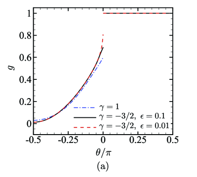
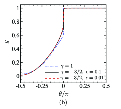
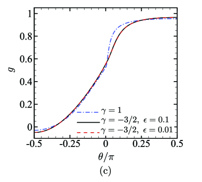
Figure 1: Reduced VDF $g$ for the finite-range ($\gamma=1$) and the cutoff potential ($\gamma=-3/2$) with $\epsilon=0.1$ and 0.01. (a) $x_{1}=-1/2$, (b) $x_{1}=-1/2+0.106\times 10^{-3}$, and (c) $x_{1}=-1/2+0.520\times 10^{-1}$.

Figure 1 shows the profiles of $g$ for the finite-range potential with $\gamma=1$ (the hard-disk) and the cutoff potential with $\gamma=-3/2$ (the cutoff Maxwell molecule). As is seen in Fig. 1(a), there is a jump discontinuity at $\theta=0$ on the boundary $x_{1}=-1/2$, which vanishes even immediately away from the boundary [Figs. 1(b) and (c)]. Figure 2(a) shows the profile of $\rho_{g}$, more precisely $|\mathrm{SE}[\rho_{g}]|=|\rho_{g}(x_{1})-\rho_{g}(-1/2)|$ divided by the distance from the boundary (see Appendix B), near the boundary for the same case as Fig. 1 with the abscissa being the logarithmic scale.

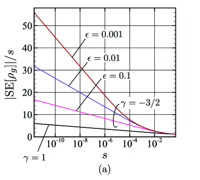
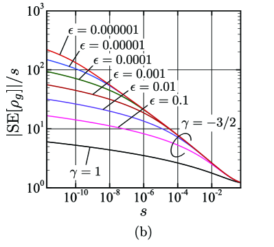
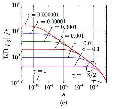
Figure 2: Variations of $\rho_{g}$ near the boundary as a function of the normal distance $s\equiv x_{1}+1/2$ from the boundary for the finite-range ($\gamma=1$) and the cutoff potential ($\gamma=-3/2$) with various sizes of cutoff $\epsilon$. (a) $|\mathrm{SE}[\rho_{g}]|/s$ in the semilog plot, (b) $|\mathrm{SE}[\rho_{g}]|/s$ in the log-log plot, and (c) $|\mathrm{KR}[\rho_{g}]|/s$.

Because it shows a nearly straight line for $s\equiv x_{1}+1/2\lesssim 10^{-6}$, $\mathrm{SE}[\rho_{g}]$ (or $\rho_{g}$) changes in proportion to $s\ln s$ from its value on the boundary. In other words, $d\rho_{g}/dx_{1}$ diverges logarithmically in approaching the boundary. Hence, the moment singularity studied in Refs. TF13 ; CLT14 ; SO73 ; CH15 is well reproduced by the present Lorentz-gas model.

Next, the results for the cutoff potential with $\gamma=-3/2$ for various values of $\epsilon$ down to $10^{-6}$ from $10^{-1}$ are shown in Figs. 2(b) and 2(c). Again, $|\mathrm{SE}[\rho_{g}]|$ divided by the distance from the boundary is shown in Fig. 2(b), but as the log-log plot. It is observed that the profiles for different $\epsilon$ forms an envelope outside the region of logarithmic change in Fig. 2(a) and that the envelope extends towards the boundary as $\epsilon$ decreases. Although it is not enough clear in Fig. 2(b), the envelope follows the power law of the distance $s$, which is clearly demonstrated in Fig. 2(c), where $|\mathrm{KR}[\rho_{g}]|$ (in place of $|\mathrm{SE}[\rho_{g}]|$) divided by the distance is shown as the log-log plot, following an efficient estimate method by Koike K21 (see Appendix B for the definition of $\mathrm{KR}$), in order to pick up the asymptotic behavior of $\rho_{g}$ near the boundary efficiently. The envelope part becomes nearly straight in Fig. 2(c) with its slope very close to $-1/5$; $|\mathrm{KR}[\rho_{g}]|$ divided by the distance is proportional to $s^{-1/5}$ there. Furthermore, the envelope extends again toward the boundary as $\epsilon\to 0$. This strongly suggests that, for the infinite range potential, the logarithmic divergence observed in the cutoff potential does not occur and instead the diverging rate becomes stronger, here $s^{-1/5}$ for $\gamma=-3/2$. In order to confirm it, the computation for the infinite-range potential with $\gamma=-3/2$ has been carried out by the Galerkin method. The result is shown in Fig. 3. The results obtained by the Galerkin method applied to the cutoff potential are also shown for comparisons with those obtained by the direct method for the reliability assessment of both methods. Excellent agreement is achieved both in Figs. 3(a) and 3(b). As expected, the envelope extends indeed down to the boundary for the infinite-range potential. From Fig. 3(b), the slope of $|\mathrm{KR}[\rho_{g}]|$ divided by the distance is estimated as $-1/5$. This confirms that $d\rho_{g}/dx_{1}$ diverges with the rate $s^{-1/5}$ in approaching the boundary (i.e., as $s\to 0$).

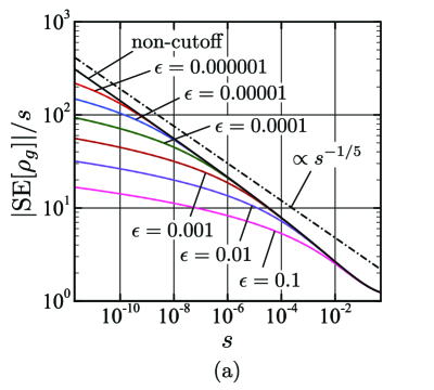
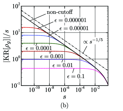
Figure 3: Variations of $\rho_{g}$ near the boundary as a function of the normal distance $s\equiv x_{1}+1/2$ from the boundary for the infinite-range and the corresponding cutoff potential ($\gamma=-3/2$). (a) $|\mathrm{SE}[\rho_{g}]|/s$ and (b) $|\mathrm{KR}[\rho_{g}]|/s$. The solid lines indicate the results by the Galerkin method. The dashed lines the results by the direct method. The latter agree well with the former and are almost invisible except for the left end in (b).

Incidentally, the computation of $|\mathrm{KR}[\rho_{g}]|$ can be sensitive to the round off errors, compared with the simpler computation of $|\mathrm{SE}[\rho_{g}]|$. Accordingly, the unnatural change of profile is observed for very small value of $s$ in the results of the direct method, because its numerical code makes use of the double precision arithmetic. Such unnatural behavior is not observed in the results of the Galerkin method, where the numerical code fully makes use of the multiple precision arithmetic with the aid of efficient libraries: exflib F by Fujiwara and Python-FLINT J by Johansson.

4.2 Discussions

In viewing the existing works for the finite-range potential, the diverging gradient of macroscopic quantities originates from the jump discontinuity of the VDF on the boundary. In this sense, it is striking that the singularity of diverging gradient occurs (more strongly) for the infinite-range potential in spite of the fact that the grazing collision regularizes $g$ to have no jump discontinuity on the boundary as shown in Fig. 4(a); see also Fig. 4(b) for other values of $\gamma$. We show below two clue observations that give the hints to this unexpected result.

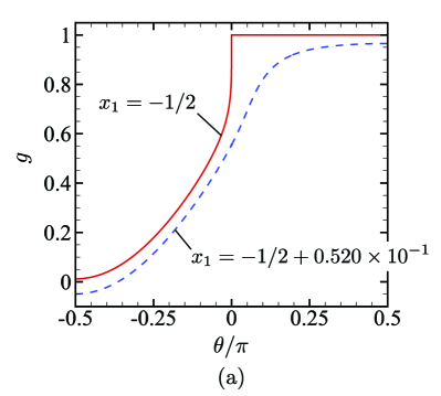
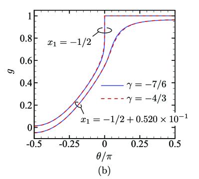
Figure 4: Reduced VDF $g$ for the infinite-range potential on and away from the boundary. (a) $\gamma=-3/2$, (b) $\gamma=-4/3$ and $-7/6$.

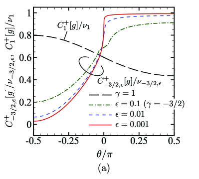
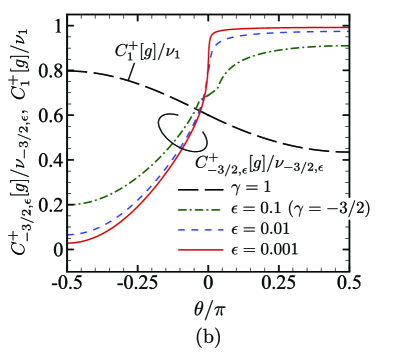
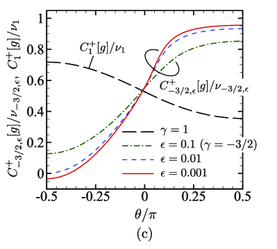
Figure 5: Gain term divided by the collision frequency for the finite-range ($\gamma=1$) and the cutoff potential ($\gamma=-3/2$) with $\epsilon=0.1,0.01,0.001$: $C_{-3/2,\epsilon}^{+}[g]/\nu_{-3/2,\epsilon}$ and $C_{1}^{+}[g]/\nu_{1}$. (a) $x_{1}=-1/2$, (b) $x_{1}=-1/2+0.106\times 10^{-3}$, and (c) $x_{1}=-1/2+0.520\times 10^{-1}$.

The first clue is the collision term $C[g]$. For the finite-range potential, the singular feature of $C[g]$ is confined in the loss term as the jump discontinuity of $g$ and the gain term $C^{+}[g]$ behaves smoothly as demonstrated in Fig. 5 (see the case $\gamma=1$). For the cutoff potential, however, $C^{+}[g]$ changes steeply for $\theta\sim 0$, losing the smooth feature observed for the finite range potential (see Fig. 5 for $\gamma=-3/2$ with small $\epsilon$). Accordingly, even after combined with the loss term, the collision integral $C[g]$ changes steeply and tends to diverge as $\theta\to 0$; see Figs. 6(a) and 6(b). Figure 6(c) shows the behavior of $C_{-3/2,\epsilon}[g]$ on the boundary for various values of $\epsilon$, which strongly suggests that $C_{-3/2}[g]$ on the boundary diverges in the limit $\theta\to 0$ with the rate $|\theta|^{-3/10}$. The grazing collision induces, even if locally, the divergence of the collision integral, as the price for regularizing the VDF. The trade-off makes the situation worse in the moment singularity.

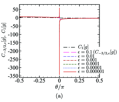
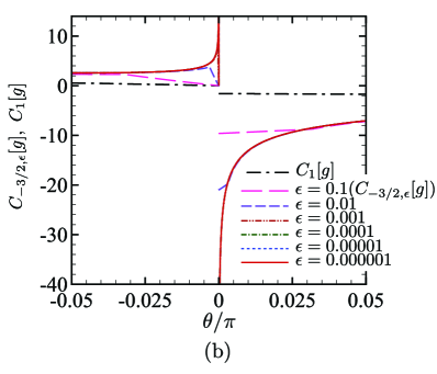
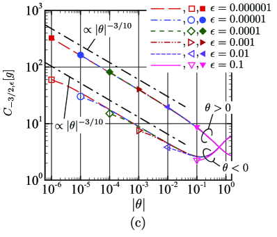
Figure 6: Collision integral for the finite-range ($\gamma=1$) and the cutoff potential ($\gamma=-3/2$) on the boundary $x_{1}=-1/2$: $C_{-3/2,\epsilon}[g]$ and $C_{1}[g]$. (a) $C_{-3/2,\epsilon}[g]$ and $C_{1}[g]$ as functions of $\theta/\pi$, (b) close-up of (a), and (c) $C_{-3/2,\epsilon}[g]$ for $|\theta|\geq\epsilon$. In (c), the data $C_{-3/2,\epsilon}[g]$ are plotted for various values of $\epsilon$ and the data at $|\theta|=\epsilon$ are indicated by a symbol.

The second clue is the correspondence among the eigenvalues $\lambda_{\pm 1},\cdots,\lambda_{\pm(2N-1)}$ and coefficients $\eta_{\pm 1},\cdots,\eta_{\pm(2N-1)}$ that occur in the exponential elements; see (46). Thanks to (22), $\rho_{g}$ is expressed as

$$\rho_{g}(x_{1})=\sum_{j=-2N}^{2N}g_{j}(x_{1})w_{j},\quad w_{j}=\frac{1}{\pi}\int_{-\pi/2}^{\pi/2}Y_{j}(\theta)d\theta.$$

Then, the substitution of (33) gives

$$\rho_{g}(x_{1})=\sum_{j\neq 0}g_{j}(x_{1})\{w_{j}-\frac{\widetilde{D}_{j}}{\widetilde{D}_{0}}w_{0}\},$$

which is further transformed by the substitution of (46) as follows:

$$\rho_{g}(x_{1}) =\sum_{j\neq 0}\Big{[}\sum_{q=1}^{2N-1}\{\eta_{q}e^{\lambda_{q}(x_{1}-\frac{1}{2})}u_{(q)j}+\eta_{-q}e^{-\lambda_{q}(x_{1}+\frac{1}{2})}u_{(-q)j}\}$$

$$\qquad\qquad+\eta_{*}\xi x_{1}u_{(0)j}+\eta_{*}u_{*j}\Big{]}\{w_{j}-\frac{\widetilde{D}_{j}}{\widetilde{D}_{0}}w_{0}\}$$

$$=\sum_{q=1}^{2N-1}\{W_{(q)}e^{\lambda_{q}(x_{1}-\frac{1}{2})}+W_{(-q)}e^{-\lambda_{q}(x_{1}+\frac{1}{2})}\}+\xi x_{1}W_{(0)}+W_{*}$$

$$=\sum_{q=1}^{2N-1}W_{(q)}\{e^{\lambda_{q}(x_{1}-\frac{1}{2})}-e^{-\lambda_{q}(x_{1}+\frac{1}{2})}\}+\xi x_{1}W_{(0)}+W_{*},$$

where

$$W_{(q)}=\sum_{j\neq 0}\{w_{j}-\frac{\widetilde{D}_{j}}{\widetilde{D}_{0}}w_{0}\}\eta_{q}u_{(q)j}=-W_{(-q)},$$

$$W_{(0)}=\sum_{j\neq 0}\{w_{j}-\frac{\widetilde{D}_{j}}{\widetilde{D}_{0}}w_{0}\}\eta_{*}u_{(0)j},\quad W_{*}=\sum_{j\neq 0}\{w_{j}-\frac{\widetilde{D}_{j}}{\widetilde{D}_{0}}w_{0}\}\eta_{*}u_{*j},$$

and $\eta_{0}=0$ has been used. Figure 7 shows $W_{(q)}$ vs $\lambda_{q}$ and $\Delta\lambda_{q}$ vs $\lambda_{q}$ for the infinite-range potential with $\gamma=-3/2$, where $\Delta\lambda_{q}=\lambda_{q}-\lambda_{q-1}$ and $\lambda_{q}$ increases indefinitely as $q\to\infty$. From the figure, it is seen that $W_{(q)}\propto\lambda_{q}^{-4/5}$ and $\Delta\lambda_{q}\propto\lambda_{q}$ as $\lambda_{q}$ (or $q$) increases. Then, as is often done in the statistical mechanics for large $N$, the summation with respect to $q$ is well estimated by the integration as $\sum_{q=1}^{2N-1}W_{(q)}e^{-a\lambda_{q}}=\int_{\lambda_{1}}^{\infty}W(\lambda)e^{-a\lambda}d\lambda$ for $a>0$, where $W$, $\lambda$, and $d\lambda$ are the appropriate continuous counterparts of $W_{(q)}/\Delta\lambda_{q}$, $\lambda_{q}$, and $\Delta\lambda_{q}$. For the present purpose of the diverging rate estimate, the lower bound of the integration range $\lambda_{1}$ may be replaced by unity, because only the behavior of the integrand for large $\lambda$ is relevant.

Hence, because of Fig. 7, $W(\lambda)\sim\lambda^{-9/5}$ for $\gamma=-3/2$, and the singular behavior of $\rho_{g}$ can be estimated by

$$\int_{1}^{\infty}\lambda^{-9/5}\exp(-\lambda s)d\lambda=\frac{5}{4}-\frac{5\pi\sec(\frac{3\pi}{10})}{4\Gamma(\frac{4}{5})}s^{4/5}+O(s).$$

By taking the derivative with respect to $s$, the diverging rate $s^{-1/5}$ of $d\rho_{g}/dx_{1}$ is reproduced.

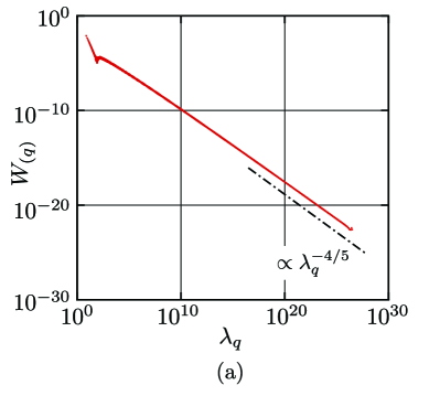
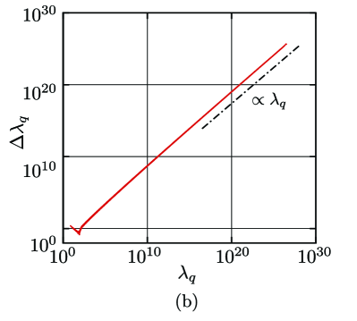
Figure 7: Weight $W_{(q)}$ and the interval of eigenvalues $\Delta\lambda_{q}$ against the eigenvalue $\lambda_{q}$ for the infinite-range potential ($\gamma=-3/2$). (a) $W_{(q)}$ and (b) $\Delta\lambda_{q}$. In the plot, the data for the grid system for $\theta$ with $N=688$ are used, where the grid points next to the origin are $\theta^{(\pm 1)}=\pm 1.05\times 10^{-17}$.

4.3 Conjecture on the Diverging Rate for Infinite-Range Potentials

From the detailed observations on the case $\gamma=-3/2$, it is conjectured for $\gamma<-1$ that

$$W(\lambda)\sim\lambda^{\frac{2}{\gamma-1}-1}=\lambda^{\frac{1}{n}-2}\quad\mbox{as }\lambda\to\infty,$$ (49)

and that the diverging rate of $d\rho_{g}/dx_{1}$ is $s^{-\frac{\gamma+1}{\gamma-1}}=s^{-1/n}$. Indeed, this conjecture recovers the second clue part of Sec. 4.2. When $\gamma=-7/6$ (or $n=13)$, it gives

$$W(\lambda)\sim\lambda^{-25/13}\quad\mbox{as }\lambda\to\infty,$$

$$\int_{1}^{\infty}\lambda^{-25/13}\exp(-\lambda s)d\lambda=\frac{13}{12}-\frac{13\pi\sec(\frac{11}{26}\pi)}{12\Gamma(\frac{12}{13})}s^{12/13}+O(s),$$

and predicts the diverging rate of $s^{-1/13}$; when $\gamma=-4/3$ (or $n=7)$, it gives

$$W(\lambda)\sim\lambda^{-13/7}\quad\mbox{as }\lambda\to\infty,$$

$$\int_{1}^{\infty}\lambda^{-13/7}\exp(-\lambda s)d\lambda=\frac{7}{6}-\frac{7\pi\sec(\frac{5}{14}\pi)}{6\Gamma(\frac{6}{7})}s^{6/7}+O(s),$$

and predicts the diverging rate of $s^{-1/7}$. The prediction rates for $\gamma=-4/3,-7/6$ are also confirmed numerically, as shown in Fig. 8.

Furthermore, when $\gamma=-2$ (or $n=3$), it gives

$$W(\lambda)\sim\lambda^{-5/3}\quad\mbox{as }\lambda\to\infty,$$

$$\int_{1}^{\infty}\lambda^{-5/3}\exp(-\lambda s)d\lambda=\frac{3}{2}-\frac{\sqrt{3}\pi}{\Gamma(\frac{2}{3})}s^{2/3}+O(s),$$

and predicts the diverging rate of $s^{-1/3}$; when $\gamma=-7/3$ (or $n=5/2$), it gives

$$W(\lambda)\sim\lambda^{-8/5}\quad\mbox{as }\lambda\to\infty,$$

$$\int_{1}^{\infty}\lambda^{-8/5}\exp(-\lambda s)d\lambda=\frac{5}{3}-\frac{5\pi\sec(\frac{\pi}{10})}{3\Gamma(\frac{3}{5})}s^{3/5}+O(s),$$

and predicts the diverging rate of $s^{-2/5}$. Although the direct numerical assessment is not available for $\gamma\leq-2$ at present, an alternative assessment is possible by numerically observing the asymptotic behavior of the envelope in $|\mathrm{KR}[\rho_{g}]|/s$ for small $\epsilon$’s by using the direct method; the results support the prediction for $\gamma=-2$ and $-7/3$; see Fig. 9.

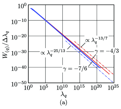
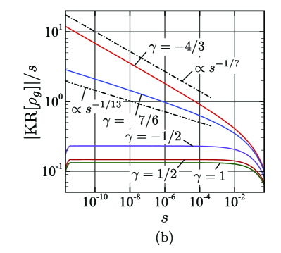
Figure 8: $W_{(q)}/\Delta\lambda_{q}$ against the eigenvalue $\lambda_{q}$ and the variation of $\rho_{g}$ near the boundary for the infinite-range potential in the case $\gamma=-4/3,-7/6$. (a) $W_{(q)}/\Delta\lambda_{q}$ and (b) $|\mathrm{KR}[\rho_{g}]|$. In (b) the cases for the finite-range potential ($\gamma=1$ and $\gamma=\pm 1/2$) are also shown for reference. For (a), see the caption of Fig. 7 as well.

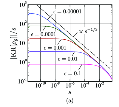
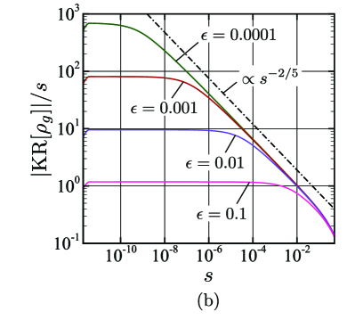
Figure 9: Variation of $\rho_{g}$ for the cutoff potential for $\gamma=-2$ and $-7/3$ with various sizes of cutoff $\epsilon$. (a) $\gamma=-2$ and (b) $\gamma=-7/3$. See (53) in Appendix B for $\mathrm{KR}[\rho_{g}]$.

To summarize, the diverging rate is logarithmic for the finite-range ($-1<\gamma\leq 1$) and the cutoff potential [see Fig. 2 and Fig. 8(b) for $\gamma=\pm 1/2$], while it is $s^{-\frac{\gamma+1}{\gamma-1}}=s^{-1/n}$ for the infinite-range potential with $-3<\gamma<-1$.

5 Conclusion

Using a mono-speed Lorentz-gas model, the moment singularity near the flat boundary has been investigated. First, the logarithmic moment singularity in approaching the boundary is checked to be reproduced for the finite-range and the cutoff potentials by the Lorentz-gas model. The jump discontinuity of the velocity distribution function is also reproduced well on the boundary. Then, by using the Galerkin method for the infinite-range potential, it is demonstrated that the grazing collision indeed has the regularizing effect on the velocity distribution function and that the jump discontinuity disappears on the boundary. Surprisingly however, the moment singularity is not weakened but rather strengthened to be of the inverse power of the distance from the boundary. This is due to the fact that the collision integral becomes locally infinite in the molecular velocity direction parallel to the boundary ($\theta=0$) as the price for the regularization of the VDF on the boundary. By detailed analyses of the high-resolution numerical data, a conjecture is made for the prediction of the diverging rate for the infinite range potential with $-3<\gamma<-1$, which are numerically confirmed for different values of $\gamma$. In conclusion, the diverging rate is logarithmic for the finite-range ($-1<\gamma\leq 1$) and the cutoff potential, while it is $s^{-\frac{\gamma+1}{\gamma-1}}=s^{-1/n}$ for the infinite-range potential with $-3<\gamma<-1$.

Finally, by the present work, it is strongly suggested that for the infinite-range potential the collision integral of the standard Boltzmann equation does not remain finite on the boundary and that the moment singularity is induced as well near the boundary. The rate expected near the planar boundary is of the inverse-power which is stronger than the logarithmic rate for the finite-range and the cutoff potential.

Appendix A Basis Functions

For the sake of the numerical convenience, the grid points in $\theta$-space are arranged to be symmetric with respect to $\theta=0$ in the region $-\pi/2\leq\theta\leq\pi/2$ so as to make $2N$ small intervals in both the positive and negative side:

$$0 =\theta^{(0)}<\theta^{(1)}<\cdots<\theta^{(2N-1)}<\theta^{(2N)}=\pi/2,\quad\theta^{(-j)}=-\theta^{(j)},\quad(j=1,\dots,2N).$$

The size of the intervals is not uniform and is smaller near $\theta=0$ so that many grid points are around there. Then the following basis function set $\{Y_{i}(\theta)\}$ ($i=-2N,\dots,2N$) is used for the piecewise quadratic approximation of a function of $\theta$:

$$Y_{2\ell}(\theta)=\begin{cases}{\displaystyle\frac{(\theta-\theta^{(2\ell+1)})(\theta-\theta^{(2\ell+2)})}{(\theta^{(2\ell)}-\theta^{(2\ell+1)})(\theta^{(2\ell)}-\theta^{(2\ell+2)})}},&\theta^{(2\ell)}<\theta<\theta^{(2\ell+2)},\ -N\leq\ell<N,\\ {\displaystyle\frac{(\theta-\theta^{(2\ell-1)})(\theta-\theta^{(2\ell-2)})}{(\theta^{(2\ell)}-\theta^{(2\ell-1)})(\theta^{(2\ell)}-\theta^{(2\ell-2)})}},&\theta^{(2\ell-2)}<\theta<\theta^{(2\ell)},\ -N<\ell\leq N,\\ 0,&\mbox{otherwise},\end{cases}$$

$$Y_{2\ell+1}(\theta)=\begin{cases}{\displaystyle\frac{(\theta-\theta^{(2\ell)})(\theta-\theta^{(2\ell+2)})}{(\theta^{(2\ell+1)}-\theta^{(2\ell)})(\theta^{(2\ell+1)}-\theta^{(2\ell+2)})}},&\theta^{(2\ell)}<\theta<\theta^{(2\ell+2)},\ -N\leq\ell<N,\\ 0,&\mbox{otherwise}.\end{cases}$$

By definition, $Y_{j}(\theta)=Y_{-j}(-\theta)$ and that $Y_{0}(\theta)$ is even in $\theta$.

In the direct method, $Y_{\pm 0}(\theta)=Y_{0}(\theta)H(\pm\theta)$ is also prepared to express the jump discontinuity of $g$ at $\theta=0$, where $H(\theta)$ is the Heaviside function. Using the notation $g_{\pm 0}(x_{1})=g(x_{1},\theta=\pm 0)$, the $g$ having a jump discontinuity at $\theta=0$ is approximated by

$$g(x_{1},\theta)=\sum_{i=1}^{2N}\{g_{-i}(x_{1})Y_{-i}(\theta)+g_{i}(x_{1})Y_{i}(\theta)\}+g_{-0}(x_{1})Y_{-0}(\theta)+g_{+0}(x_{1})Y_{+0}(\theta).$$ (50)

If there is no jump discontinuity, $g$ is simply approximated by $g=\sum_{i=-2N}^{2N}g_{i}Y_{i}(\theta)$ with the simplified notation $g_{0}(x_{1})\equiv g_{\pm 0}(x_{1})$. Accordingly, the numerical kernel used in the direct method takes the form $C^{+}[g]=\sum_{i=1}^{2N}\{g_{-i}C^{+}[Y_{-i}]+g_{i}C^{+}[Y_{i}]\}+g_{-0}C^{+}[Y_{-0}]+g_{+0}C^{+}[Y_{+0}]$ or $C^{+}[g]=\sum_{i=-2N}^{2N}g_{i}C^{+}[Y_{i}]$, depending on whether the jump discontinuity exists or not.

The analytical expression of $C^{+}[Y_{i}]$ is available with the aid of the series expansion of $|\sin\frac{\varphi}{2}|^{\gamma}$. Although it is truncated by a finite number of terms, the expression is helpful to perform the accurate numerical computation. The same applies to the Galerkin method, i.e., both $A_{ij}$ and $D_{ij}$ can be obtained analytically as well even for the infinite-range potential. The highly accurate computations with the multiple precision arithmetic are achieved in this way.

Appendix B Acceleration Method for Estimating the Asymptotic Behavior

In the present study, an acceleration method proposed in Ref. K21 that makes use of the Richardson extrapolation is found to be very powerful in estimating the asymptotic behavior of the density in approaching the boundary. The method is briefly explained in this appendix.

Suppose that a function $f$ of $x(\geq X)$ behaves

$$f(x)\sim f(X)+a_{\alpha}s^{\alpha}+a_{1}s+o(s),$$ (51)

for $x\sim X$, where $s=x-X$ and $0<\alpha<1$ is an unknown constant. In the application to the present work, put $X=-1/2$. The idea of the method is composed of killing the third term to clearly pick up the second term on the right-hand side, thereby improving the estimate of the exponent $\alpha$ by the linear regression on the log-log plot.

The straightforward estimate (SE) for the exponent $\alpha$ is just to take

$$\mathrm{SE}[f]\equiv f(x)-f(X)\sim a_{\alpha}s^{\alpha}+a_{1}s+o(s),$$ (52)

and to use the linear regression. As is clear from the most-right-hand side, however, the $O(s)$ term may affect the linear regression unless a clear difference of scale appears in the data at hands. In Ref. K21 , the following combination of $f$ that makes use of the Richardson extrapolation is proposed by Koike (the KR method, for short):

$$\mathrm{KR}[f]\equiv f(x)-2f(X+s/2)+f(X).$$ (53)

Then, it behaves

$$\mathrm{KR}[f]\sim a_{\alpha}(1-2^{1-\alpha})s^{\alpha}+o(s),$$

and accordingly there is no longer influence of the term $O(s)$ in the linear regression. Hence, the estimate of $\alpha$ should be improved.

Practically, there is a possible drawback such that $\mathrm{KR}[f]$ would require more significant digits than $\mathrm{SE}[f]$ in order to avoid the influence of the round-off error. Indeed, in Figs. 2(c) and 3(b), the influence can be observed in the results by the direct method but not in the results by the Galerkin method. The difference comes from that the computation code for the former uses the double precision arithmetic, while that for the latter uses the multiple precision arithmetic and does not make a discretization in $x_{1}$.

- (1) Kogan, M. N.: Rarefied Gas Dynamics, Plenum Press, New York (1969).
- (2) Sone, Y.: Molecular Gas Dynamics, Birkhäuser, Boston (2007); supplementary notes and errata are available from KURENAI (http://hdl.handle.net/2433/66098).
- (3) Takata, S., Taguchi, S.: Gradient divergence of fluid-dynamic quantities in rarefied gases on smooth boundaries, J. Stat. Phys. 168, 1319–1352 (2017). https://doi.org/10.1007/s10955-017-1850-7.
- (4) Takata, S., Funagane, H.: Singular behaviour of a rarefied gas on a planar boundary, J. Fluid Mech. 717, 30–47 (2013). https://doi.org/10.1017/jfm.2012.559.
- (5) Chen, I.-K., Liu, T.-P., Takata, S.: Boundary singularity for thermal transpiration problem of the linearized Boltzmann equation, Arch. Rational Mech. Anal. 212, 575–595 (2014). https://doi.org/10.1007/s00205-013-0714-9.
- (6) Taguchi, S., Saito, K., Takata, S.: A rarefied gas flow around a rotating sphere: diverging profiles of gradients of macroscopic quantities, J. Fluid Mech. 862, 5–33 (2019). https://doi.org/10.1017/jfm.2018.946.
- (7) Chen, I.-K., Hsia, C.-H.: Singularity of macroscopic variables near boundary for gases with cutoff hard potential, SIAM J. Math. Anal. 47, 4332–4349 (2015).
- (8) Cercignani, C.: The Boltzmann Equation and Its Applications, Springer, Berlin (1988). http://dx.doi.org/10.1007/978-1-4612-1039-9.
- (9) Desvillettes, L.: About the regularizing properties of the non-cut-off Kac equation, Commun. Math. Phys. 168, 417–440 (1995). https://doi.org/10.1007/BF02101556.
- (10) Desvillettes, L., Golse, F.: On a model Boltzmann equation without angular cutoff, Differential and Integral Equations 13, 567–594 (2000).
- (11) Villani, C.: A review of mathematical topics in collisional kinetic theory, in Handbook of Mathematical Fluid Dynamics, Vol. I, Friedlander, S., Serre, D. eds., Chapter 2 (2002). https://www.sciencedirect.com/science/handbooks/18745792/1.
- (12) Alexandre, R., Villani, C.: On the Boltzmann equation for long-range interactions, Commun. Pure Appl. Math. 55, 30–70 (2002). https://doi.org/10.1002/cpa.10012.
- (13) Mouhot, C., Strain, R. M.: Spectral gap and coercivity estimates for linearized Boltzmann collision operators without angular cutoff, J. Math. Pures Appl. 87, 515–535 (2007). https://doi.org/10.1016/j.matpur.2007.03.003.
- (14) Alexandre, R., Morimoto, Y., Ukai, S., Xu, C.-J., Yang, T.: Regularizing effect and local existence for the non-cutoff Boltzmann equation, Arch. Rational Mech. Anal. 198, 39–123 (2010). https://doi.org/10.1007/s00205-010-0290-1.
- (15) Alexandre, R., Morimoto, Y., Ukai, S., Xu, C.-J., Yang, T.: Global existence and full regularity of the Boltzmann equation without angular cutoff, Commun. Math. Phys. 304, 513–581 (2011). https://doi.org/10.1007/s00220-011-1242-9
- (16) Gressman, P. T., Strain, R. M.: Global classical solutions of the Boltzmann equation without angular cut-off, J. American Math. Soc. 24, 771–847 (2011). https://doi.org/10.1090/S0894-0347-2011-00697-8.
- (17) Chen, Y., He, L.-B.: Smoothing estimates for Boltzmann equation with full-range interactions: Spatially homogeneous case, Arch. Rational Mech. Anal. 201, 501–548 (2011). doi: 10.1007/s00205-010-0393-8
- (18) Jiang, J.-C., Liu, T.-P.: Boltzmann collision operator for the infinite range potential: A limit problem, Ann. I. H. Poincaré 36, 1639–1677 (2019). https://doi.org/10.1016/j.anihpc.2019.03.001
- (19) Takata, S.: A toy-model study of the grazing collisions in the kinetic theory, J. Stat. Phys. 160, 770–792 (2015). https://doi.org/10.1007/s10955-015-1259-0.
- (20) Bird, G. A.: Molecular Gas Dynamics and the Direct Simulation of Gas Flows, Clarendon Press, Oxford (1994).
- (21) Sone, Y., Ohwada, T., Aoki, K.: Temperature jump and Knudsen layer in a rarefied gas over a plane wall: Numerical analysis of the linearized Boltzmann equation for hard-sphere molecules, Phys. Fluids A 1, 363–370 (1989). https://doi.org/10.1063/1.857457.
- (22) Hattori, M., Takata, S.: Second-order Knudsen-layer analysis for the generalized slip-flow theory I, Bulletin of the Institute of Mathematics, Academia Sinica (New Series) 10, 423–448 (2015).
- (23) Kessler, T., Rjasanow, S.: Fully conservative spectral Galerkin–Petrov method for the inhomogeneous Boltzmann equation, Kinetic & Related Models 12, 507–549 (2019). doi: 10.3934/krm.2019021.
- (24) Sone, Y., Onishi, Y.: Kinetic theory of evaporation and condensation, J. Phys. Soc. Jpn 35, 1773–1776 (1973) https://doi.org/10.1143/JPSJ.35.1773; ibid, Kinetic theory of evaporation and condensation—Hydrodynamic equation and slip boundary condition—, J. Phys. Soc. Jpn 44, 1981–1994 (1978). https://doi.org/10.1143/JPSJ.44.1981.
- (25) Sone, Y.: Kinetic theory analysis of linearized Rayleigh problem, J. Phys. Soc. Jpn 19, 1463–1473 (1964). https://doi.org/10.1143/JPSJ.19.1463
- (26) Koike, K.: Refined pointwise estimates for a 1D viscous compressible flow and the long-time behavior of a point mass, RIMS Kôkyûroku, Appendix A.1 (to be published).
- (27) As of May 20, 2021, the library is available from http://www-an.acs.i.kyoto-u.ac.jp/~fujiwara/exflib/.
- (28) As of May 20, 2021, the library is available from https://fredrikj.net/python-flint/#.