Forecasting VaR and ES using a joint quantile regression and implications in portfolio allocation

Abstract

In this paper we propose a multivariate quantile regression framework to forecast Value at Risk (VaR) and Expected Shortfall (ES) of multiple financial assets simultaneously, extending Taylor (2019). We generalize the Multivariate Asymmetric Laplace (MAL) joint quantile regression of Petrella and Raponi (2019) to a time-varying setting, which allows us to specify a dynamic process for the evolution of both VaR and ES of each asset. The proposed methodology accounts for the dependence structure among asset returns. By exploiting the properties of the MAL distribution, we then propose a new portfolio optimization method that minimizes the portfolio risk and controls for well-known characteristics of financial data. We evaluate the advantages of the proposed approach on both simulated and real data, using weekly returns on three major stock market indices. We show that our method outperforms other existing models and provides more accurate risk measure forecasts compared to univariate ones.

Keywords: Quantile Regression, Multiple quantiles, Multivariate Asymmetric Laplace Distribution, CAViaR, Value at Risk, Expected Shortfall

1 Introduction

The events of the ongoing credit crisis and past financial crises have emphasized the necessity for appropriate risk measures. The use of quantitative risk measures has become an essential management tool providing advice, analysis and support for financial and asset management decisions to market participants and regulators. The most widely used risk measure is Value at Risk (VaR). VaR measures the maximum loss which a financial operator can incur over a defined time horizon and for a given confidence level. Its clear meaning and computational ease made it very popular among practitioners, so much so that it has largely contaminated the banking regulatory framework. However, VaR has a number of drawbacks (Artzner et al. 1997, 1999). First, VaR does not account for tail risk, i.e. it does not warn us about the size of the losses that occur with a probability lower than the predetermined confidence level. Second, VaR is not a “coherent” risk measure (Artzner et al. 1999) since it does not satisfy the sub-additivity property, and hence, it does not take into consideration the benefits of diversification. As a result, investors and risk managers are likely to construct positions with unintended weaknesses that result in greater losses under conditions beyond the VaR level (Yamai and Yoshiba 2005). Market participants could solve such problems by adopting the Expected Shortfall (ES) risk measure, which is defined as the conditional expectation of exceedances beyond VaR (see Acerbi and Tasche (2002) and Rockafellar and Uryasev (2000)). Unlike VaR, ES is a coherent risk measure and provides more information on the shape and the heaviness of the tails of the loss distribution. Therefore, ES has gained increasing attention from risk managers, banking regulators and investors as an alternative measure of risk, complementing the VaR measure.

However, despite its interesting properties, and in contrast with VaR, little work exists on modeling ES. This is in part due to the fact that ES is not an “elicitable” measure, in the sense that there does not exist a loss function such that ES is the solution that minimizes the expected loss. Several works have been proposed in the literature to overcome the problem of elicitability (see, e.g., Engle and Manganelli (2004), Cai and Wang (2008), Taylor (2008), Zhu and Galbraith (2011), Du and Escanciano (2017), Patton et al. (2019), Bu et al. (2019)). Recently, using the results of Fissler and Ziegel (2016), who show that ES is jointly elicitable with VaR, Taylor (2019) uses the Asymmetric Laplace (AL) distribution to jointly estimate dynamic models for both VaR and ES. In particular, Taylor (2019) shows that the negative of the log-likelihood associated to the AL distribution belongs to the class of loss functions presented in Fissler and Ziegel (2016), and hence it can be used to estimate and forecast VaR and ES measures in one step. In his paper, the joint estimation of VaR and ES is obtained in a univariate quantile regression framework, exploiting the interesting result that ES can be expressed in terms of the scale parameter of the AL density.

The literature mentioned above, however, has mainly focused on univariate time series, which completely disregards the strong interrelation among assets in financial markets. To capture the degree of tail interdependence between assets, several quantile-based methods have also been proposed to estimate VaR, without however specifying a model for the ES component; see, for example, the relevant works by Baur (2013); Bernardi et al. (2015); White et al. (2015); Kraus and Czado (2017) and Bonaccolto et al. (2019).

In this paper, we extend the univariate approach of Taylor (2019) to a multivariate framework, with the objective of obtaining joint estimates of both VaR and ES for multiple financial assets simultaneously, accounting for their dependence structure. To this end, we generalize the Multivariate Asymmetric Laplace (MAL) quantile regression approach of Petrella and Raponi (2019) to a time-varying setting, by allowing the parameters of the MAL to vary over time. For each asset, we model the evolution of VaR and ES as functions of the location and scale parameters of the distribution. In particular, for the VaR component, we adopt a Conditional Autoregressive Value at Risk (CAViaR) specification (Engle and Manganelli (2004)).

The advantages of our methodology are manifold. Firstly, our approach is a joint modelling framework where both the model parameters and the pair (VaR, ES) of multiple returns are estimated simultaneously, generalizing the univariate results of Bassett et al. (2004) and Taylor (2019). Secondly, our theory captures empirical characteristics of financial data such as peakedness, skewness, and heavy tails (see e.g., Kraus and Litzenberger (1976); Friend and Westerfield (1980) and Barone-Adesi (1985)), without relying on the limitation of normally distributed returns.

The inferential problem is solved by developing a suitable Expectation-Maximization (EM) algorithm, which exploits the mixture representation of the MAL distribution (see Petrella and Raponi (2019)) properly generalized to the case of time-varying parameters. The finite sample properties of the proposed estimation method are also evaluated using a simulation exercise, where we show the validity and the robustness of our procedure under different data generating processes.

A further contribution of the paper concerns the evaluation of VaR and ES in the context of portfolio optimization (see, e.g, Yiu (2004) and Alexander and Baptista (2008)). In recent years, the MAL density has attracted wide attention in the literature for its flexibility in modeling financial data (Mittnik and Rachev (1991); Kotz et al. (2012) and Paolella (2015)) and for its interesting properties that can be exploited to derive optimal portfolio allocations (see Zhao et al. (2015) and Shi et al. (2018)). In the classic Mean-Variance (MV) methodology of Markowitz (1952), portfolio risk is measured using the standard deviation of the portfolio. However, the MV approach is reasonably applicable only in cases where either returns follow a Gaussian distribution or the investors utility function is quadratic. Given the empirical evidence showing that market participants have a preference for positive skewness and they are more concerned about the downside risk (see Arditti (1971) and Konno and Suzuki (1995) among others), the MAL distribution could represents a more effective tool to select optimal portfolio allocations in the case of risk-averse agents. Therefore, in this paper we exploit the MAL properties to incorporate skewness directly into the portfolio optimization method and to identify the optimal allocation weights. We then compute the corresponding portfolio VaR and ES as a function of the multivariate structure of the data. We prove how this result follows directly from the fact that any linear combination of the MAL components is still AL distributed, with location, skew and scale parameters that are functions of the MAL parameters and the portfolio weights. Therefore, once we obtain the Maximum Likelihood (ML) estimates of the MAL parameters from the proposed dynamic quantile regression model, we fix a desired level of risk for any target portfolio and search for the optimal allocation weights according to the adopted strategy.

Specifically, we consider the Skewness Mean-Variance (SMV) strategy of Zhao et al. (2015), where the optimal allocation is obtained by minimizing the portfolio variance, while controlling for the skewness of asset returns. However, Zhao et al. (2015) employed the method of moments to estimate the portfolio variance; on the contrary, we estimate the MAL parameters in a ML framework by using an EM algorithm.

Empirically, we analyze weekly returns of the FTSE 100, NIKKEI 225 and Standard $\&$ Poor’s 500 (S&P 500) market indices from April 1985 to February 2021. In a first out-of-sample exercise we jointly estimate the VaR and ES of the three stock market indices using the proposed dynamic joint quantile regression model, hence taking into account for the correlation among the three indices. To evaluate VaR and ES forecasts and to show the main advantages of the proposed method, we use different backtesting procedures, where we compare the out-of-sample VaR and ES predictions with the ones obtained by applying the univariate method of Taylor (2019). In particular, to perform a joint evaluation of VaR and ES, we follow Fissler et al. (2015), Nolde et al. (2017), Patton et al. (2019) and Taylor (2019) and extend their approach by introducing a new scoring function based on the MAL distribution. We find that our multivariate method always provides more accurate VaR and ES predictions compared to other well-known approaches, like the Quantile AutoRegression of Koenker and Xiao (2006) and the dynamic quantile regression of Taylor (2019). Moreover, in line with Taylor (2019), our results show that the Asymmetric Slope CAViaR specification of Engle and Manganelli (2004) yields the best VaR and ES forecasts for all the three indices at different quantile levels, confirming the existence of relevant asymmetries in the impact of positive and negative returns.

In a second empirical analysis, we aggregate the stock market indices to form a financial portfolio with a predetermined level of risk, and estimate its optimal allocation weights by implementing our new optimization procedure. We then compute the out-of-sample portfolio’s VaR and ES and evaluate the predictions using the univariate backtesting procedures of Taylor (2019), Nolde et al. (2017) and Patton et al. (2019). The empirical analysis reveals that our multivariate method produces the lowest average losses compared to other existing strategies based on the multivariate Normal and t- distributions, regardless of the scoring function being used. In addition, we find that the proposed methodology overall yields the highest Sharpe Ratio and the least concentrated portfolio allocations.

The rest of the paper is organized as follows. In Section 2, we introduce the dynamic multiple quantile regression and propose a joint model for VaR and ES. We then illustrate the EM-based ML approach for the simultaneous estimation of VaR and ES. Section 3 develops the portfolio allocation problem. Section 4 introduces a new scoring function for the joint evaluation of VaR and ES forecasts. In Section 5 we discuss the main empirical results, while Section 6 concludes. All the proofs are provided in Appendix A, while the simulation study is presented in Appendix B.

2 Multivariate framework

In this paper we generalize the univariate regression approach of Taylor (2019). Specifically, by extending the MAL density of Petrella and Raponi (2019) – allowing the location and scale parameters of the MAL to vary over time – we estimate the pair of VaR and ES associated to each asset using a joint quantile regression framework. In this way, we are able to calculate the time-varying VaR and ES simultaneously for all marginal response variables, accounting for possible correlation among the considered assets. For the VaR components, we assume a CAViaR specification (see Engle and Manganelli (2004)). Parameter estimation is carried out using a suitable EM algorithm as in Petrella and Raponi (2019), properly extended to deal with the time-varying setting. In this way, the estimated parameters account for tail interdependence among multiple returns and convey this information onto the VaR and ES estimates.

We start by introducing the time-varying joint quantile regression model in Section 2.1, where we consider a dynamic generalization of the MAL density proposed in Petrella and Raponi (2019). We then show in Section 2.2 how the resulting time-varying scale parameter of the MAL can be used to model the ES vector and derive a parsimonious approach for simultaneous estimation of VaR and ES in a multidimensional setting. Parameter estimation and the EM algorithm are described in Section 2.3.

2.1 Dynamic joint quantile regression

Let $\boldsymbol{Y}_{t}=[Y_{t1},Y_{t2},...,Y_{tp}]^{\prime}$ be a $p$-variate response variable and denote by ${\cal Q}_{Y_{tj}}(\tau_{j}|\mathcal{F}_{t-1})$ the $\tau_{j}$-quantile function of each of the $j$-th component of $\boldsymbol{Y}_{t}$, conditional on the information set $\mathcal{F}_{t-1}$ available at time $t-1$, for $j=1,...,p$ and $t=1,...,T$. Then, for a given $\tau_{j}$, we consider the following autoregressive dynamic:

$${\cal Q}_{Y_{tj}}(\tau_{j}|\mathcal{F}_{t-1})=\omega_{j}+\eta_{j}{\cal Q}_{Y_{t-1j}}(\tau_{j}|\mathcal{F}_{t-2})+\ell(\boldsymbol{\beta}_{j},Y_{t-1j}),$$ (1)

where $\omega_{j}=\omega_{j}(\tau_{j})$, $\eta_{j}=\eta_{j}(\tau_{j})$ and $\boldsymbol{\beta}_{j}=\boldsymbol{\beta}_{j}(\tau_{j})=[\beta_{1j},...,\beta_{Kj}]^{\prime}$ are model parameters that depend on the chosen level $\tau_{j}$ and where we suppress the index $\tau_{j}$ for simplicity of notation. The dynamic specification in (1) is well-known in the literature as the CAViaR model of Engle and Manganelli (2004), which attempts to compute the $\tau$-th level VaR by estimating the $\tau$-th level quantile of the asset returns through a conditional autoregressive structure. The function $\ell(\cdot)$ represents the so-called News Impact Curve (NIC), originally introduced by Engle and Ng (1993). For each $j$-th component, the NIC function essentially feeds back the last available observation ($Y_{t-1j}$) into the present value of the conditional quantile, through the $K\times 1$ parameter vector $\boldsymbol{\beta}_{j}$. Following the CAViaR literature, we will consider different specifications for $\ell(\cdot)$ to model the marginal quantiles, which will be described in the next section.

Using matrix notation, the representation in (1) can be embedded in the following multivariate linear regression model:

$$\boldsymbol{Y}_{t}=\boldsymbol{\mu}_{t}+\boldsymbol{\epsilon}_{t},\quad\quad t=1,2,...,T$$ (2)

where $\boldsymbol{\epsilon}_{t}$ denotes a $p\times 1$ vector of error terms, having each marginal quantile (at fixed levels $\tau_{1},..,\tau_{p}$, respectively) equal to zero, to ensure that $\boldsymbol{\mu}_{t}={\cal Q}_{\boldsymbol{Y}_{t}}(\boldsymbol{\tau}|\mathcal{F}_{t-1})$.

To estimate the regression model in (2), we consider a dynamic generalization of the MAL distribution introduced in Petrella and Raponi (2019) and Kotz et al. (2012), i.e. we consider the time-varying distribution $\mbox{MAL}_{p}\left(\boldsymbol{\mu}_{t},\boldsymbol{D}_{t}\boldsymbol{\tilde{\xi}},\,\boldsymbol{D}_{t}\boldsymbol{\tilde{\Sigma}}\boldsymbol{D}_{t}\right)$, with density function:

$$f_{\boldsymbol{Y}_{t}}(\boldsymbol{y}_{t}|\boldsymbol{\mu}_{t},\boldsymbol{D}_{t}\boldsymbol{\tilde{\xi}},\boldsymbol{D}_{t}\boldsymbol{\tilde{\Sigma}}\boldsymbol{D}_{t},\mathcal{F}_{t-1})=\frac{2\exp{\left\{(\boldsymbol{y}_{t}-\boldsymbol{\mu}_{t})^{\prime}\boldsymbol{D}_{t}^{-1}\boldsymbol{\tilde{\Sigma}}^{-1}\boldsymbol{\tilde{\xi}}\right\}}}{(2\pi)^{p/2}|\boldsymbol{D}_{t}\boldsymbol{\tilde{\Sigma}}\boldsymbol{D}_{t}|^{1/2}}\left(\frac{\tilde{m}_{t}}{2+\tilde{d}}\right)^{\nu/2}K_{\nu}\left(\sqrt{(2+\tilde{d})\tilde{m}_{t}}\right).$$

In (2.1), $\boldsymbol{\mu}_{t}$ represents the location parameter vector, $\boldsymbol{D}_{t}\boldsymbol{\tilde{\xi}}\in{\mathcal{R}}^{p}$ is the scale (or skew) parameter, with $\boldsymbol{D}_{t}=\mbox{diag}[\delta_{t1},\delta_{t2},...,\delta_{tp}]$, $\delta_{tj}>0$ and $\boldsymbol{\tilde{\xi}}=[\tilde{\xi}_{1},\tilde{\xi}_{2},...,\tilde{\xi}_{p}]^{\prime}$, having generic element $\tilde{\xi}_{j}=\frac{1-2\tau_{j}}{\tau_{j}(1-\tau_{j})}$. $\boldsymbol{\tilde{\Sigma}}$ is a $p\times p$ positive definite matrix such that $\boldsymbol{\tilde{\Sigma}}=\boldsymbol{\tilde{\Lambda}}\boldsymbol{\Psi}\boldsymbol{\tilde{\Lambda}}$, with $\boldsymbol{\Psi}$ having the structure of a correlation matrix and $\boldsymbol{\tilde{\Lambda}}=\mbox{diag}[\tilde{\sigma}_{1},\tilde{\sigma}_{1},...,\tilde{\sigma}_{p}]$, with $\tilde{\sigma}_{j}^{2}=\frac{2}{\tau_{j}(1-\tau_{j})}$, $j=1,...,p$. Moreover, $\tilde{m}_{t}=(\boldsymbol{y}_{t}-\boldsymbol{\mu}_{t})^{\prime}(\boldsymbol{D}_{t}\boldsymbol{\tilde{\Sigma}}\boldsymbol{D}_{t})^{-1}(\boldsymbol{y}_{t}-\boldsymbol{\mu}_{t})$, $\tilde{d}=\boldsymbol{\tilde{\xi}}^{\prime}\boldsymbol{\tilde{\Sigma}}^{-1}\boldsymbol{\tilde{\xi}}$, and $K_{\nu}(\cdot)$ denotes the modified Bessel function of the third kind with index parameter $\nu=(2-p)/2$.

Notice that, as stressed in Petrella and Raponi (2019), the specification in (2.1) should not be viewed as a parametric assumption in model (2), but rather a convenient tool to jointly estimate marginal dynamic quantiles of a multivariate response variable in a quantile regression framework. Moreover, as clarified in their paper, the constraints $\tilde{\xi}_{j}=\frac{1-2\tau_{j}}{\tau_{j}(1-\tau_{j})}$ and $\tilde{\sigma}_{j}^{2}=\frac{2}{\tau_{j}(1-\tau_{j})}$ need to be imposed to guarantee model identifiability (see Petrella and Raponi (2019), Proposition 2), and also to ensure that the dynamic quantile specification in (1) holds, i.e. $\mathbb{P}(Y_{tj}<\mu_{tj})=\tau_{j}$ holds for each $j=1,2,...,p$.

In addition, when such constraints are satisfied, then each marginal component of the MAL in (2.1) follows a univariate AL distribution, that is $Y_{tj}\sim\textnormal{AL}(\mu_{tj},\tau_{j},\delta_{tj})$, where $\delta_{tj}$ represents the time-varying scale parameter of $Y_{tj}$. This allows us to exploit the result of Taylor (2019), who shows the link between the scale parameter of the AL distribution and the ES risk measure in a univariate framework. By extending these results, we provide new insights on how to estimate conditional VaR and ES jointly in a multidimensional setting, that accounts for correlations between marginals. This is explained in details in the next section.

2.2 Modeling VaR and ES jointly

Following Engle and Manganelli (2004), the CAViaR specification in (1) allows us to derive the VaR of an asset at level $\tau_{j}$ by estimating the corresponding quantile at the $\tau_{j}$-th level, through a conditional autoregressive structure. In the following, we consider several CAViaR formulations, depending on the choice of the NIC function $\ell(\cdot)$. We then extend the idea of Taylor (2019) to a multivariate setting, in order to model and estimate the ES component dynamically.

The CAViaR specifications that we consider are the following:

$${\cal Q}_{Y_{tj}}(\tau_{j}|\mathcal{F}_{t-1}) = \omega_{j}+\eta_{j}{\cal Q}_{Y_{t-1j}}(\tau_{j}|\mathcal{F}_{t-2})+\beta_{1j}|Y_{t-1j}|,\quad\quad\textit{Symmetric Absolute Value (SAV)}$$

$${\cal Q}_{Y_{tj}}(\tau_{j}|\mathcal{F}_{t-1}) = \omega_{j}+\eta_{j}{\cal Q}_{Y_{t-1j}}(\tau_{j}|\mathcal{F}_{t-2})+\beta_{1j}Y^{+}_{t-1j}+\beta_{2j}Y^{-}_{t-1j},\quad\quad\textit{Asymmetric Slope (AS)}$$

$${\cal Q}_{Y_{tj}}(\tau_{j}|\mathcal{F}_{t-1}) = \left(\omega_{j}+\eta_{j}{\cal Q}^{2}_{Y_{t-1j}}(\tau_{j}|\mathcal{F}_{t-2})+\beta_{2j}Y^{2}_{t-1j}\right)^{1/2}\quad\quad\textit{Indirect GARCH(1,1) (IG)}$$

where $\boldsymbol{\omega}=[\omega_{1},...,\omega_{p}]^{\prime},\boldsymbol{\eta}=[\eta_{1},...,\eta_{p}]^{\prime}$ and $\boldsymbol{\beta}=[\boldsymbol{\beta}_{1},...,\boldsymbol{\beta}_{p}]^{\prime}$, with $\boldsymbol{\beta}_{j}=[\beta_{1j},\beta_{2j}]^{\prime}$, are unknown parameters to be estimated, and where $y^{+}=\max(y,0)$ and $y^{-}=-\min(y,0)$, denote the positive and negative part of $y$, respectively.

For the ES component, we exploit the interesting link provided in Bassett et al. (2004), which relates univariate quantile regression to conditional ES through the following relation:

$$ES_{tj}=\mathbb{E}[Y_{tj}]-\frac{\mathbb{E}[(Y_{tj}-{\cal Q}_{Y_{tj}})(\tau_{j}-\boldsymbol{1}_{(Y_{tj}<{\cal Q}_{Y_{tj}})})]}{\tau_{j}}$$ (7)

with $\boldsymbol{1}(\cdot)$ being the indicator function. Following Taylor (2019), the expression in (7) can be rearranged so that the conditional ES can be expressed in terms of the conditional AL scale parameter $\delta_{tj}$. Specifically, recalling that each marginal of the MAL distribution has a univariate AL density with conditional scale parameter equal to $\delta_{tj}={\mathbb{E}[(Y_{tj}-{\cal Q}_{Y_{tj}})(\tau_{j}-\boldsymbol{1}_{(Y_{tj}<{\cal Q}_{Y_{tj}})})]}$, then equation (7) reduces to:

$$ES_{tj}=\mathbb{E}[Y_{tj}]-\frac{\delta_{tj}}{\tau_{j}},\quad\quad t=1,2,...,T,\quad j=1,2,...,p$$ (8)

implying that

$$\delta_{tj} = {\tau_{j}}\left(\mathbb{E}[Y_{tj}]-ES_{tj}\right),\quad\quad t=1,2,...,T,\quad j=1,2,...,p$$ (9)

In order to ensure that each estimated ES does not cross the corresponding estimated quantile, we model ES in (9) as the product of the quantile and a constant factor (see, e.g., Gourieroux et al. (2012) and Taylor (2019)) as follows:

$$ES_{tj}=(1+e^{\gamma_{0j}}){\cal Q}_{Y_{tj}}(\tau_{j}),\quad\quad t=1,2,...,T,\quad j=1,2,...,p,$$ (10)

where $\gamma_{0j}$ is an unconstrained parameter to be estimated such that $1+e^{\gamma_{0j}}$ is greater than 1 and $\boldsymbol{Y}_{t}$ is assumed with zero mean. We collect the unknown parameters in the vector $\boldsymbol{\gamma}_{0}=[\gamma_{01},...,\gamma_{0p}]^{\prime}$. As explained in Taylor (2019), this formulation correctly describes the relationship between ES and VaR for different data generating processes, such as a GARCH process with a Student-t distribution. Therefore, the representation in (10) provides a simple and parsimonious approach to estimate VaR and ES simultaneously in a dynamic framework.

In (10), however, only the quantile is dynamic, while the factor $1+e^{\gamma_{0j}}$ remains constant through time. Therefore, in order to generalize this approach, we also consider the alternative formulation for the ES presented in Taylor (2019), where the difference between the ES and the VaR is modeled using an AutoRegressive (AR) specification as follows:

$$ES_{tj} ={\cal Q}_{Y_{tj}}(\tau_{j})-x_{tj},\quad\quad t=1,2,...,T,\quad j=1,2,...,p,$$ (11)

$$x_{tj} =(\gamma_{1j}+\gamma_{2j}({\cal Q}_{Y_{t-1j}}(\tau_{j})-Y_{t-1j})+\gamma_{3j}x_{t-1j})\boldsymbol{1}_{(Y_{tj}\leq{\cal Q}_{Y_{tj}})}+x_{t-1j}\boldsymbol{1}_{(Y_{tj}>{\cal Q}_{Y_{tj}})},$$ (12)

where we define the nonnegative parameter $\boldsymbol{\gamma}=[\boldsymbol{\gamma}_{1},...,\boldsymbol{\gamma}_{p}]^{\prime}$, with $\boldsymbol{\gamma}_{j}=[\gamma_{1j},\gamma_{2j},\gamma_{3j}]^{\prime}$, to ensure that the VaR and ES estimates do not cross.

In the next section, we show how to estimate model parameters using a ML approach based on a dynamic modification of the EM algorithm proposed by Petrella and Raponi (2019).

2.3 Parameter estimation using the EM algorithm

Before describing the main steps of the EM algorithm, we first introduce the notation $\boldsymbol{\cal Q}_{t}={\cal Q}_{\boldsymbol{Y}_{t}}(\boldsymbol{\tau}|\mathcal{F}_{t-1})$, $\boldsymbol{D}_{t}(\boldsymbol{\gamma})$ and ${\boldsymbol{\tilde{\Sigma}}}(\boldsymbol{\Psi})$ to make clear that the vector ${\cal Q}_{\boldsymbol{Y}_{t}}(\boldsymbol{\tau}|\mathcal{F}_{t-1})$ and the matrices $\boldsymbol{D}_{t}$ and $\boldsymbol{\tilde{\Sigma}}$ depend on the unknown parameters $\boldsymbol{\omega},\boldsymbol{\eta},\boldsymbol{\beta},\boldsymbol{\gamma}$ and $\boldsymbol{\Psi}$, respectively. The derivation of the EM algorithm is based on the Proposition 3 of Petrella and Raponi (2019), properly extended to deal with the autoregressive structure of the quantile function $\boldsymbol{\cal Q}_{t}$ and the time dependency of the scale matrix $\boldsymbol{D}_{t}(\boldsymbol{\gamma})$.

Let ${\boldsymbol{\Phi}}=\{\boldsymbol{\omega},\boldsymbol{\eta},\boldsymbol{\beta},\boldsymbol{\gamma},{\boldsymbol{\Psi}}\}$ denote the global set of parameters and define ${\boldsymbol{\hat{\Phi}}}=\{\boldsymbol{\hat{\omega}},\boldsymbol{\hat{\eta}},\boldsymbol{\hat{\beta}},\boldsymbol{\hat{\gamma}},{\boldsymbol{\hat{\Psi}}}\}$ as the corresponding set of parameter estimates. For a given vector $\boldsymbol{\tau}=[\tau_{1},\tau_{2},...,\tau_{p}]^{\prime}$, the expected complete log-likelihood function (up to additive constants), given the observed data $\boldsymbol{Y}_{t}$ and the parameter estimates ${\boldsymbol{\hat{\Phi}}}$, is:

[]

$$E\left[\l_{c}({\boldsymbol{\Phi}}|\boldsymbol{Y}_{t},\boldsymbol{\hat{\Phi}})\right]=-\frac{1}{2}\sum_{t=1}^{T}\log|\boldsymbol{D}_{t}{({\boldsymbol{\gamma}})}\tilde{\boldsymbol{\Sigma}}{(\boldsymbol{\Psi})}\boldsymbol{D}_{t}{({\boldsymbol{\gamma}})}|+\sum_{t=1}^{T}(\boldsymbol{Y}_{t}-\boldsymbol{\cal Q}_{t})^{\prime}\boldsymbol{D}_{t}{({\boldsymbol{\gamma}})}^{-1}\tilde{\boldsymbol{\Sigma}}{(\boldsymbol{\Psi})}^{-1}\tilde{\boldsymbol{\xi}}$$ (13)

[]

$$-\frac{1}{2}\sum_{t=1}^{T}z_{t}(\boldsymbol{Y}_{t}-\boldsymbol{\cal Q}_{t})^{\prime}(\boldsymbol{D}_{t}{({\boldsymbol{\gamma}})}\tilde{\boldsymbol{\Sigma}}{({\boldsymbol{\Psi}})}\boldsymbol{D}_{t}{({\boldsymbol{\gamma}})})^{-1}(\boldsymbol{Y}_{t}-\boldsymbol{\cal Q}_{t})$$ (14)

$$-\frac{1}{2}\tilde{{\boldsymbol{\xi}}}^{\prime}\tilde{\boldsymbol{\Sigma}}{(\boldsymbol{\Psi})}^{-1}\tilde{\boldsymbol{\xi}}\sum_{t=1}^{T}u_{t},$$ (15)

where

$${u}_{t} = E[W_{t}|\boldsymbol{Y}_{t},\boldsymbol{\hat{\Phi}}]=\left(\frac{\hat{\tilde{m}}_{t}}{2+\hat{\tilde{d}}}\right)^{\frac{1}{2}}\frac{K_{\nu+1}\left(\sqrt{(2+\hat{\tilde{d}})\hat{\tilde{m}}_{t}}\right)}{K_{\nu}\left(\sqrt{(2+\hat{\tilde{d}})\hat{\tilde{m}}_{t}}\right)}$$ (16)

$${z}_{t} = E[W_{t}^{-1}|\boldsymbol{Y}_{t},\boldsymbol{\hat{\Phi}}]=\left(\frac{2+\hat{\tilde{d}}}{\hat{\tilde{m}}_{t}}\right)^{\frac{1}{2}}\frac{K_{\nu+1}\left(\sqrt{(2+\hat{\tilde{d}})\hat{\tilde{m}}_{t}}\right)}{K_{\nu}\left(\sqrt{(2+\hat{\tilde{d}})\hat{\tilde{m}}_{t}}\right)}-\frac{2\nu}{\hat{\tilde{m}}_{t}},$$ (17)

with

$$\hat{\tilde{m}}_{t} = (\boldsymbol{y}_{t}-\boldsymbol{\cal Q}_{t})^{\prime}(\boldsymbol{D}_{t}{(\hat{\boldsymbol{\gamma}})}\tilde{\boldsymbol{\Sigma}}{(\hat{\boldsymbol{\Psi}})}\boldsymbol{D}_{t}{(\hat{\boldsymbol{\gamma}})})^{-1}(\boldsymbol{y}_{t}-\boldsymbol{\cal Q}_{t}),\qquad\hat{\tilde{d}}=\tilde{\boldsymbol{\xi}}^{\prime}\tilde{\boldsymbol{\Sigma}}{(\hat{\boldsymbol{\Psi}})}^{-1}\tilde{\boldsymbol{\xi}},$$ (18)

and where $W_{t}$ follows a standard exponential distribution.

For a given vector $\boldsymbol{\tau}$, the expected complete log-likelihood in (13)-(15) is then maximized with respect to the parameter set $\boldsymbol{\Phi}$, yielding to the M-step updates ${\boldsymbol{\hat{\Phi}}}=\{\boldsymbol{\hat{\omega}},\boldsymbol{\hat{\eta}},\boldsymbol{\hat{\beta}},\boldsymbol{\hat{\gamma}},{\boldsymbol{\hat{\Psi}}}\}$. Notice that, unlike Petrella and Raponi (2019), closed form solutions for $\boldsymbol{\hat{\omega}},\boldsymbol{\hat{\eta}},\boldsymbol{\hat{\beta}}$ and $\boldsymbol{\hat{\gamma}}$ do not exist, due to the autoregressive structure of the data and, therefore, numerical optimization is required. Updated estimates of $\boldsymbol{\tilde{\Sigma}}(\boldsymbol{\hat{\Psi}})$ can be instead derived using the following expression:

[]

$${\tilde{\boldsymbol{\Sigma}}}{(\hat{\boldsymbol{\Psi}})} =\frac{1}{T}\sum_{t=1}^{T}{z}_{t}\boldsymbol{D}_{t}{(\hat{\boldsymbol{\gamma}})}^{-1}(\boldsymbol{Y}_{t}-\boldsymbol{\cal Q}_{t})(\boldsymbol{Y}_{t}-\boldsymbol{\cal Q}_{t})^{\prime}\boldsymbol{D}_{t}{(\hat{\boldsymbol{\gamma}})}^{-1}$$ (19)

$$+\frac{1}{T}\sum_{t=1}^{T}{u}_{t}\tilde{\boldsymbol{\xi}}\tilde{\boldsymbol{\xi}}^{\prime}-\frac{2}{T}\sum_{t=1}^{T}\boldsymbol{D}_{t}{(\hat{\boldsymbol{\gamma}})}^{-1}(\boldsymbol{Y}_{t}-\boldsymbol{\cal Q}_{t})\tilde{\boldsymbol{\xi}}^{\prime}.$$ (20)

Therefore, the EM algorithm can be implemented as follows:

E-step: Set the iteration number $h=1$. Fix the vector $\boldsymbol{\tau}$ at the chosen quantile levels $\tau_{1},...,\tau_{p}$ of interest and initialize the parameter set ${\boldsymbol{\Phi}}=\{\boldsymbol{\omega},\boldsymbol{\eta},\boldsymbol{\beta},\boldsymbol{\gamma},{\boldsymbol{\Psi}}\}$. Then, given $\boldsymbol{\hat{\Phi}}=\boldsymbol{\hat{\Phi}}^{(h)}=\{\boldsymbol{\hat{\omega}}^{(h)},\boldsymbol{\hat{\eta}}^{(h)},\boldsymbol{\hat{\beta}}^{(h)},\boldsymbol{\hat{\gamma}}^{(h)},\boldsymbol{\hat{\Psi}}^{(h)}\}$, at each iteration $h$ calculate the weights:

$$\hat{u}^{(h)}_{t} = \left(\frac{\hat{\tilde{m}}^{(h)}_{t}}{2+\hat{\tilde{d}}^{(h)}}\right)^{\frac{1}{2}}\frac{K_{\nu+1}\left(\sqrt{(2+\hat{\tilde{d}}^{(h)})\hat{\tilde{m}}^{(h)}_{t}}\right)}{K_{\nu}\left(\sqrt{(2+\hat{\tilde{d}}^{(h)})\hat{\tilde{m}}^{(h)}_{t}}\right)}$$ (21)

$$\hat{z}^{(h)}_{t} = \left(\frac{2+\hat{\tilde{d}}^{(h)}}{\hat{\tilde{m}}^{(h)}_{t}}\right)^{\frac{1}{2}}\frac{K_{\nu+1}\left(\sqrt{(2+\hat{\tilde{d}}^{(h)})\hat{\tilde{m}}^{(h)}_{t}}\right)}{K_{\nu}\left(\sqrt{(2+\hat{\tilde{d}}^{(h)})\hat{\tilde{m}}^{(h)}_{t}}\right)}-\frac{2\nu}{\hat{\tilde{m}}^{(h)}_{t}}$$ (22)

where

$$\hat{\tilde{m}}^{(h)}_{t} = (\boldsymbol{y}_{t}-\boldsymbol{\cal Q}_{t}^{(h)})^{\prime}(\boldsymbol{D}_{t}{(\hat{\boldsymbol{\gamma}}^{(h)})}\tilde{\boldsymbol{\Sigma}}{(\hat{\boldsymbol{\Psi}}^{(h)})}\boldsymbol{D}_{t}{(\hat{\boldsymbol{\gamma}}^{(h)})})^{-1}(\boldsymbol{y}_{t}-\boldsymbol{\cal Q}_{t}^{(h)}),$$ (23)

$$\hat{\tilde{d}}^{(h)} = \tilde{\boldsymbol{\xi}}^{\prime}\tilde{\boldsymbol{\Sigma}}{(\hat{\boldsymbol{\Psi}}^{(h)})}^{-1}\tilde{\boldsymbol{\xi}}.$$ (24)

M-step: Use the estimates $\hat{u}^{(h)}_{t}$ and $\hat{z}^{(h)}_{t}$ to maximize $E[\l_{c}(\boldsymbol{\Phi}|\boldsymbol{\hat{\Phi}}^{(h)})]$ with respect to $\boldsymbol{\Phi}$, and obtain the updated set of parameter estimates $\boldsymbol{\hat{\Phi}}^{(h+1)}$.

The optimization procedure is iterated until convergence, that is when the difference between the likelihood function evaluated at two consecutive iterations is smaller than $10^{-5}$. We initialize the EM algorithm by providing the univariate parameter estimates of Taylor (2019) on each asset, while the initial value for the correlation matrix $\boldsymbol{\Psi}$ in (2.1) is calibrated using the empirical correlation matrix of the data. We fit the univariate models following the estimation procedure in Engle and Manganelli (2004) and Taylor (2019). In addition, we also consider a multiple random starts strategy with 100 different starting points to better explore the parameter space, and retain the solution corresponding to the maximum likelihood value. This strategy would prevent convergence issues and avoid the algorithm to be trapped at some local maxima. From an algorithmic point of view, the EM method exploits the Nelder-Mead and the Broyden-Fletcher-Goldfarb-Shanno (BFGS) optimization routines to obtain the updated estimates of $\boldsymbol{\beta}$ and $\boldsymbol{\gamma}$, meanwhile it uses (19) to compute the updated estimate of $\boldsymbol{\tilde{\Sigma}}$.
The computational analysis has been conducted using the R (version 4.0.2) software where the functions to update $\boldsymbol{\beta}$, $\boldsymbol{\gamma}$ and $\boldsymbol{\tilde{\Sigma}}$ were coded in efficient C++ object-oriented programming.
The validity and the performance of the proposed EM algorithm have been assessed using also a simulation exercise (see Appendix B).

3 Portfolio Construction

In this section we approach the problem of portfolio allocation. Particularly, we construct the Skewness Mean-Variance (SMV) portfolio of Zhao et al. (2015), taking into account both for the multivariate structure and the skewness of asset returns. Following Stolfi et al. (2018) and Zhao et al. (2015), we exploit an interesting property characterizing the MAL distribution in (2.1). Specifically, we show that any linear combination of its marginal components follows a univariate AL distribution, whose parameters are a function of the MAL parameters in (2.1). Note that, while the MAL density has so far been regarded as a convenient tool for estimating the marginal quantiles, in this section the MAL distribution is used as a data driven assumption to describe the empirical characteristics of asset returns. As already stated in the Introduction, this choice has been positively accepted in the recent financial literature to detect peakedness, fat-tail, and skewness of financial assets, overcoming possible deficiencies of standard approaches relying, for example, on the Gaussian distribution assumption. We then evaluate the riskiness of the selected portfolio by calculating its corresponding VaR and ES, using the results of Section 2.2.

3.1 Linear combinations of MAL components

Let assume that $\boldsymbol{Y}_{t}$ is a $p$-dimensional random variable describing the joint dynamics of $p$ variables at time $t$. Let us consider a linear combination (with weights to be determined) of each component of $\boldsymbol{Y}_{t}$. Then, the following proposition holds.

Proposition 1.

Let $\boldsymbol{Y}_{t}\sim\mbox{MAL}_{p}(\boldsymbol{\mu}_{t},\boldsymbol{D}_{t}\boldsymbol{\tilde{\xi}},\boldsymbol{D}_{t}\boldsymbol{\tilde{\Sigma}}\boldsymbol{D}_{t})$, with density function defined in (2.1). Let $\boldsymbol{b}_{t}=(b_{t1},...,b_{tp})^{\prime}\in{\cal R}^{p}$ be a vector of weights such that $\boldsymbol{b}_{t}\neq\boldsymbol{0}_{p}$, with $\boldsymbol{0}_{p}$ denoting a $p$-vector of zeros. Define the random variable $Y_{t}^{\boldsymbol{b}}=\sum_{j=1}^{p}b_{tj}Y_{tj}$. Then,

$$Y_{t}^{\boldsymbol{b}}\sim\mbox{AL}(\mu_{t}^{\star},\tau_{t}^{\star},\delta_{t}^{\star})$$ (25)

where

$$\mu_{t}^{\star}=\boldsymbol{b_{t}^{\prime}\mu_{t}}\mbox{,}\quad\tau_{t}^{\star}=\frac{1}{2}(1-\frac{\boldsymbol{b_{t}^{\prime}D_{t}\tilde{\xi}}}{\sqrt{2(\boldsymbol{b_{t}^{\prime}D_{t}\tilde{\Sigma}D_{t}b_{t}})+(\boldsymbol{b_{t}^{\prime}D_{t}\tilde{\xi}})^{2}}})\quad\textnormal{and}\quad\delta_{t}^{\star}=\frac{(\boldsymbol{b_{t}^{\prime}D_{t}\tilde{\Sigma}D_{t}b_{t}})}{2{\sqrt{2(\boldsymbol{b_{t}^{\prime}D_{t}\tilde{\Sigma}D_{t}b_{t}})+(\boldsymbol{b_{t}^{\prime}D_{t}\tilde{\xi}})^{2}}}}.$$

Proposition 1 brings out two main considerations. First, the distribution of $Y_{t}^{\boldsymbol{b}}$ is still AL, which greatly facilitates the computation of the VaR and the ES in our context. Second, the parameters of $Y_{t}^{\boldsymbol{b}}$ are expressed as a function of the multivariate parameters $\boldsymbol{\mu}_{t},\boldsymbol{D}_{t}$ and $\boldsymbol{\tilde{\Sigma}}$ of the MAL in (2.1). This allows us to take into account the possible association among the marginal components of ${\boldsymbol{Y}_{t}}$ when choosing the allocation weights $\boldsymbol{b}_{t}$. In the next section, we exploit such property to retrieve the returns distribution of a financial portfolio, whose optimal weights can be derived by solving a simple constrained optimization problem. Given the resulting optimal portfolio weights, we can then use the results of Section 2.2 to derive appropriate measures of portfolio’s VaR and ES.

3.2 The portfolio optimization problem

Assume that $\boldsymbol{Y}_{t}$ follows the distribution in (2.1). Given such specification, at each time $t$, investors might be interested in deriving a portfolio $Y^{b}_{t}=\sum_{j=1}^{p}b_{tj}Y_{tj}$, by investing a portion $b_{tj}$ of their capital on the asset $Y_{tj}$, such that $\sum_{j=1}^{p}b_{tj}=1$. Then, under this setting, the result of Proposition 1 can be easily applied, yielding a portfolio with location, skewness and scale parameters equal to, respectively, $\mu^{\star}_{t}$, $\tau^{\star}_{t}$ and $\delta_{t}^{\star}$ as in (1).

Typically, in risk management applications, the skewness parameter is fixed a priori by the researcher at a certain level (constant over time) $\tau^{\star}_{t}=\tilde{\tau}$, as it essentially measures the overall riskiness of a financial product (a portfolio, in our case). Therefore, once we estimate the time-varying MAL parameters from the quantile regression model in (2), for a fixed level of risk $\tilde{\tau}$, the investor’s portfolio decision is based on the solution of the selected portfolio strategy. As stated above, to obtain the optimal portfolio allocation, we adopt the SMV strategy of Zhao et al. (2015), which seeks to minimize the portfolio variance and at the same time control for the skewness of asset returns. Formally, according to Proposition 1, the SMV portfolio solves the following constrained optimization problem:

$$\underset{\boldsymbol{b}_{t}\in\mathcal{R}^{p}}{{\rm argmin}} \quad\boldsymbol{b}_{t}^{\prime}\boldsymbol{D}_{t}\boldsymbol{\tilde{\Sigma}}\boldsymbol{D}_{t}\boldsymbol{b}_{t}$$ (27a)

s.t. $$\quad\tau_{t}^{\star}=\tilde{\tau},\quad\forall t$$ (27b)

$$\quad\boldsymbol{b}^{\prime}_{t}\boldsymbol{1}_{p}=1$$ (27c)

where $\boldsymbol{\tilde{\Sigma}}$ has been introduced in (2.1) and accounts for the covariance matrix of the returns, while $\boldsymbol{b}_{t}$ denotes the portfolio’s weights at time $t$ held by the investor over the period $[t,t+1)$.

From an empirical point of view, the constraint in (27b) implies that the portfolio weights must be adjusted at each holding period to guarantee that the VaR of the portfolio has constant level $\tilde{\tau}$, namely $\mathbb{P}(Y^{\boldsymbol{b}}_{t}<\mu^{\star}_{t}|\mathcal{F}_{t-1})=\tilde{\tau}$. Once we obtain the optimal portfolio weights for the period $[t,t+1)$, we can then compute the conditional portfolio’s VaR and ES at level $\tilde{\tau}$ by simply applying the result in (8) to the univariate case.

As already explained above, since the parameters $\mu_{t}^{\star},\tau_{t}^{\star},\delta_{t}^{\star}$ depend on the parameter estimates of the MAL, information on the dependence structure and on the empirical characteristics embedded in the data is channeled through such estimates into the portfolio’s VaR and ES forecasts. This motivates our approach even further, since it could offer an operative and useful tool to help investors and asset managers in deriving optimal portfolio allocations and, at the same time, monitoring multiple VaR and ES jointly.

4 Assessment of VaR and ES forecasts

To assess the performance of VaR and ES predictions jointly, we introduce a new backtesting procedure, based on the multivariate approach discussed in Section 2.

Backtesting techniques are based on quantitative tests which scrutinize model performance in terms of accuracy and precision with respect to a defined criterion. Existing approaches, however, rely on tests that analyze VaR and ES predictions separately, i.e. they only focus on the individual evaluation of one risk measure or the other. VaR evaluation is typically based on coverage tests, which measure the percentage of times that the returns have exceeded the estimated VaR at a chosen probability level $\tau$ (see, e.g., the unconditional coverage (LR_uc) test of Kupiec (1995), the conditional coverage (LR_cc) test of Christoffersen (1998) and the Dynamic Quantile (DQ) test of Engle and Manganelli (2004)).

To evaluate ES forecasts, the backtesting analysis becomes more complicated since ES is not an elicitable measure (Gneiting, 2011) and, therefore, suitable scoring functions cannot be determined (Taylor, 2019). The test of McNeil and Frey (2000) is commonly used in this context, which is based on the discrepancy between the observed return and the ES forecast for the periods in which the return exceeds the VaR forecast. Another suitable option is the backtesting procedure of Du and Escanciano (2017) which is based on the Unconditional ES (U_ES) and Conditional ES (C_ES) tests.

However, since ES relies on observations exceeding the VaR, it is clear that assessment of ES forecasts cannot be independent of the predicted VaR values. This, together with the fact that ES is not elicitable, motivates the introduction of a scoring function for jointly evaluating VaR and ES forecasts. Based on the characterization of consistent scoring functions introduced by Fissler and Ziegel (2016) and Nolde et al. (2017), several scoring rules have been proposed in the literature for the univariate setting (see, e.g., Patton et al. (2019), Fissler et al. (2015) and Taylor (2019)).

In the following, we provide a new scoring rule that can be used in a multivariate setting, to jointly evaluate VaR and ES forecasts of multiple (and possibly correlated) financial assets. To provide support for our proposal of estimating multiple VaR and ES by maximizing the MAL likelihood, we define a new scoring function ($S_{MAL}$) using the negative of the MAL log score:

$$\begin{aligned} S_{MAL}\left(\boldsymbol{\cal Q}_{t},\boldsymbol{ES}_{t},\boldsymbol{y}_{t};\boldsymbol{\tilde{\Sigma}},\boldsymbol{\tau}\right)=\frac{1}{2}\log\left(|\boldsymbol{\tilde{\Sigma}}|\right)+\log\left(|(\boldsymbol{\tau}\boldsymbol{ES}_{t}^{\prime})\circ\textnormal{{I}}_{p}|\right)-\frac{\nu}{2}\log\left(\frac{\tilde{m}_{t}}{2+\tilde{d}}\right)\\ +(\boldsymbol{y}_{t}-\boldsymbol{\cal Q}_{t})^{\prime}{\left((\boldsymbol{\tau}\boldsymbol{ES}_{t}^{\prime})\circ\textnormal{{I}}_{p}\right)}^{-1}\boldsymbol{\tilde{\Sigma}}^{-1}\boldsymbol{\tilde{\xi}}-\log\left(K_{\nu}\left(\sqrt{(2+\tilde{d})\tilde{m}_{t}}\right)\right)\end{aligned}$$ (28)

where $\circ$ denotes the Hadamard product and $\textnormal{{I}}_{p}$ represents the identity matrix of order $p$.

Notice that, when $p$ is equal to 1, the $S_{MAL}$ in (28) reduces to the AL log score of Taylor (2019). When $p>1$, the loss function $S_{MAL}$ allows us to: (i) perform a joint assessment of the pairs (VaR, ES) specific to each asset and, at the same time, (ii) control for the existing correlation among returns.

5 Empirical Study

In this section we apply the methodology presented in Sections 2 and 3 to real data in order to evaluate and compare its empirical implications with the ones obtained by using a univariate framework. Particularly, we follow Taylor (2019) and use weekly returns of the FTSE 100, NIKKEI 225, and S&P 500 stock market indices, from April 26, 1985 to February 01, 2021. Using a rolling window exercise, we estimate the one-week-ahead VaR and ES forecasts implied by the CAViaR specifications described in Section 2.2, and select the most desirable model using the Diebold and Mariano (2002) test. In a second empirical exercise, we aggregate the market indices to form a financial portfolio and determine its optimal allocation weights by solving the optimization problem described in Section 3.2. We finally compute and assess the resulting portfolio’s conditional VaR and ES for the out-of-sample period, which consists of the last 368 observations of the sample.

5.1 Data

Our sample is collected from Bloomberg and it consists of 1868 weekly returns for each of the three stock indices. The main summary statistics are displayed below in Table 1, providing evidence of the well-known stylized facts on fat tails, high kurtosis, serial and cross-sectional correlation that typically characterize financial assets. Moreover, all series exhibit a negative skewness, the Jarque-Bera test significantly rejects the normality assumption, the Ljung-Box test advocates the presence of serial correlation and the Augmented Dickey-Fuller test supports the hypothesis of absence of unit roots. These results clearly motivate us to consider a quantile regression approach as investigative tool.

5.2 Out-of-sample VaR and ES forecasting

Using the approach introduced in Section 2, in this section we derive a joint estimation of VaR and ES for the three stock market indices described above. Particularly, we estimate the out-of-sample series of VaR and ES by considering the three different specifications in (LABEL:SAV), (LABEL:AS) and (LABEL:IG), with both the multiplicative factor in (10) and the AR formulation in (11)-(12) for the ES component. Moreover, since we are concerned with the downside risk, we evaluate the out-of-sample forecasts at three different probability levels, namely $\boldsymbol{\tau}=[0.1,0.1,0.1],\boldsymbol{\tau}=[0.05,0.05,0.05]$ and $\boldsymbol{\tau}=[0.01,0.01,0.01]$.

The first objective is to assess the performance of the CAViaR specifications using the proposed multivariate framework. We start by evaluating the VaR forecasts using the conventional LR_uc, LR_cc and the DQ tests, while we perform the U_ES and C_ES tests of Du and Escanciano (2017) to evaluate the ES predictions. The results are shown in Table 2, where Panel A refers to the case of the ES vector modeled as in (10), while Panel B refers to the AR specification in (11)-(12). Looking at VaR forecasts, in both panels, for all the three indices and for all the three quantile levels, we find that the CAViaR-AS specification is always successfully backtested at the 5% significance level. The results are less clear, instead, for the other two CAViaR specifications. The same results are confirmed when evaluating the ES predictions, as the CAViaR-AS specification yields again outstanding performances for all the three indices and for all the three quantile levels.
To jointly evaluate VaR and ES forecasts associated to each stock market index, in addition to the results of the coverage tests, Table 3 reports the values of the loss functions $S_{FZN}$ of Nolde et al. (2017) and $S_{FZ0}$ of Patton et al. (2019), averaged over the out-of-sample period where:

$$S_{FZN}({\cal Q}_{t},ES_{t},y_{t})=(\mathbf{1}_{(y_{t}<{\cal Q}_{t})}-\tau)\frac{{\cal Q}_{t}}{2\tau\sqrt{-ES_{t}}}-\frac{1}{2\sqrt{-ES_{t}}}(\mathbf{1}_{(y_{t}<{\cal Q}_{t})}\frac{y_{t}}{\tau}-ES_{t})+\sqrt{-ES_{t}}$$ (29)

and

$$S_{FZ0}({\cal Q}_{t},ES_{t},y_{t})=\frac{1}{\tau ES_{t}}\mathbf{1}_{(y_{t}<{\cal Q}_{t})}(y_{t}-{\cal Q}_{t})+\frac{{\cal Q}_{t}}{ES_{t}}+\log(-ES_{t})-1.$$ (30)

The losses in (29) and (30) belong to the class of scoring rules proposed in Nolde et al. (2017) and Patton et al. (2019) and have the additional advantage of generating loss differences (between competing forecasts) that are homogeneous of degree $1/2$ and zero, respectively.
Overall, the results show that both the CAViaR-AS and CAViaR-IG dynamics are associated with smaller losses compared to the CAViaR-SAV model, except for the case of $\boldsymbol{\tau}=[0.1,0.1,0.1]$. Moreover, in line with Taylor (2019), we find evidence of a better forecasting performance when using the constant multiplicative factor $(1+e^{\gamma_{0j}})$ to model the ES parameter (Panel A), compared to the AR dynamics (Panel B).
Finally, to reinforce our analysis, we evaluate the forecasting performance of the three CAViaR competing models using the scoring function in (28). Specifically, at each time $t$, and for the specified level $\boldsymbol{\tau}$, we define by $S_{MAL_{t}}^{(j)}(\boldsymbol{\tau})$ the scoring function associated to model $j$, and denote the difference between the scoring function of model $i$ and model $j$ by $\Delta_{MAL,t}^{(i,j)}=S_{MAL_{t}}^{(i)}(\boldsymbol{\tau})-S_{MAL_{t}}^{(j)}(\boldsymbol{\tau})$, where $i,j=1,2,3$. We then test for the null hypothesis that $\mathbb{E}[\Delta_{MAL,t}^{(i,j)}]=0$ against $\mathbb{E}[\Delta_{MAL,t}^{(i,j)}]<0$ using the Diebold and Mariano (2002) test, for all the pairs of models $i$ and $j$. If the null hypothesis is rejected, then forecasts delivered by model $i$ are more accurate than those of model $j$, and therefore model $i$ is preferable than model $j$. The results of the test, together with the corresponding p-values, are reported in Table 4. The table clearly shows that the CAViaR-AS specification outperforms both the CAViaR-IG and CAViaR-SAV models at all the three quantile levels and for both the adopted ES formulations of constant multiplicative factor (Panel A) and AR dynamics (Panel B). Therefore, in order to select the best performing model between the two CAViaR-AS in Panels A and B, we apply again the Diebold and Mariano (2002) test on the two competing CAViaR-AS specifications. The results are reported in Table 5 and suggest that the CAViaR-AS model with the ES specified as a constant multiple of the VaR provides the most accurate predictions at all the three quantile levels. This is in line with Taylor (2019), who also find that the same specification not only produces the smallest losses, but it also delivers the most accurate predictions than all the other competing CAViaR dynamics. These results corroborate the fact that accounting for asymmetries in the autoregressive process of a given quantile improves the model’s forecasting ability (see, e.g., Engle and Manganelli (2004), Xiliang and Xi (2009), Taylor (2005) and Laporta et al. (2018)).

To show the advantages and the different implications of our approach, we compare our results with the ones obtained by considering each asset separately, as if we ignored their possible dependence structure. Specifically, the three CAViaR models are estimated individually for each stock market index using the univariate approach of Taylor (2019). To assess the performance of the three models and to combine the individual forecasts of the three indices in a single value, we use the sum of the three corresponding AL log scores (see Taylor (2019)) as consistent scoring rule. That is, at each time $t$, and for each model $j$, we define the following scoring function:

$$S_{AL_{t}}^{(j)}(\boldsymbol{\tau})=\sum_{p=1}^{3}S_{AL_{p,t}}^{(j)}(\tau_{p})$$ (31)

where $S_{AL_{p,t}}^{(j)}(\tau_{p})$ denotes the AL log-score of Taylor (2019), corresponding to model $j$ and asset $p$:

$$S_{AL_{p,t}}^{(j)}(\tau_{p})=-\log\left(\frac{\tau_{p}-1}{ES^{(j)}_{p,t}}\right)-\frac{\left(y_{p,t}-{\cal Q}_{p,t}^{(j)}\right)\left(\tau_{p}-\mathbf{1}_{(y_{p,t}<{\cal Q}_{p,t}^{(j)})}\right)}{\tau_{p}ES_{p,t}^{(j)}}.$$ (32)

As explained in Frongillo and Kash (2015), summing up the three AL scoring functions would produce a consistent scoring rule in this case, since each function $S_{AL_{p,t}}^{(j)}(\tau_{p})$ elicits the pair (VaR, ES) for the corresponding $p$-th asset (see Fissler and Ziegel (2016) and Taylor (2019)).

Then, as before, we define the difference between the scoring function of model $i$ and model $j$ by $\Delta_{AL,t}^{(i,j)}=S_{AL_{t}}^{(i)}(\boldsymbol{\tau})-S_{AL_{t}}^{(j)}(\boldsymbol{\tau})$ and apply the Diebold and Mariano (2002) test to look for the best model in terms of forecasting accuracy. The results are reported in Table 6 (Panels A and B). As shown in the table, the conclusion of the test is now less clear and does not provide any significant evidence in favor of a particular model. This is one of the first advantages of our approach, as we are able to identify a clear hierarchy among competing models.

A second question of interest concerns the “efficiency gain” of the multiple approach compared to the univariate one. In this sense, we would like to test whether taking into account the association structure among the market indices would provide us with better predictions in terms of VaR and ES. To do that, we use the backtesting procedure to identify the most “efficient” model, that is, the model producing the best forecasts according to the Diebold and Mariano (2002) test. To measure the efficiency gain we analyze the difference, if any, in the predictive accuracy between the forecast (VaR, ES) produced by our multivariate approach and the univariate ones. Therefore, for a given CAViaR specification, we test for the difference between the scores obtained with the scoring rule in (31) and the ones obtained with (28). The null hypothesis is that, on average, the difference is not statistically different from zero, i.e. the two approaches have the same forecasting performance. The alternative hypothesis is that the difference is smaller than zero, i.e. the multivariate approach delivers significantly better predictions (smaller losses).

Table 7 shows the resulting test statistics and the corresponding p-values for each of the possible pairs of competing models. Interestingly, for all the considered risk levels and for all the three CAViaR specifications, we are always able to reject the null hypothesis at 5% level, providing evidence of the efficiency gain of our proposed joint approach.

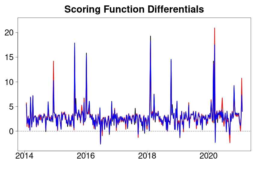
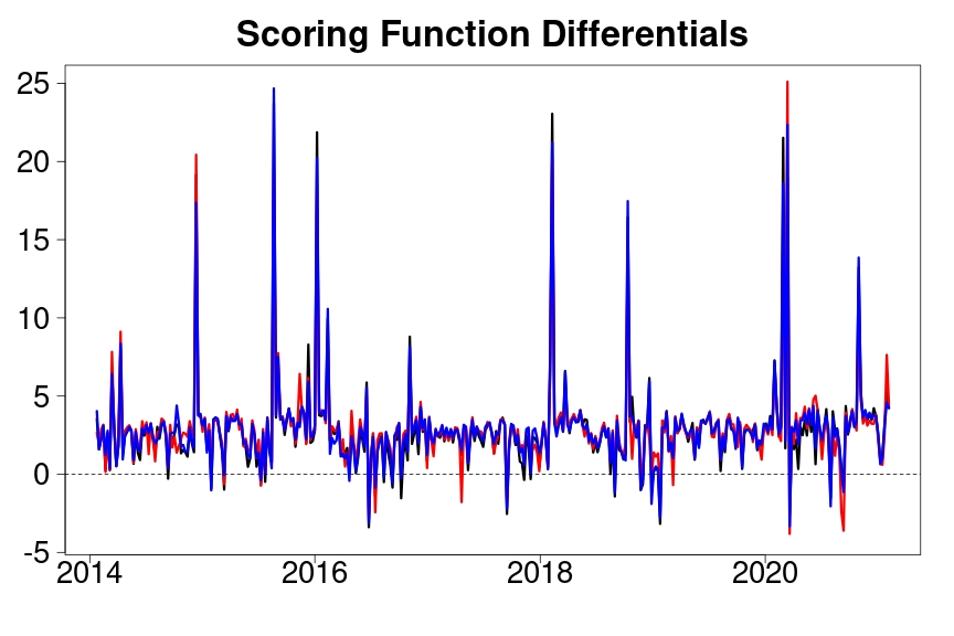
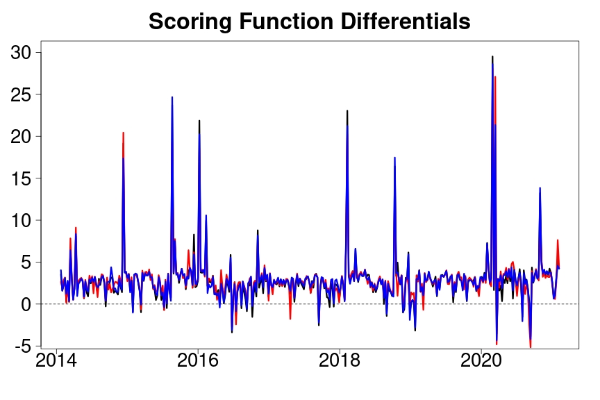
To offer a graphical intuition of the results, Figure 1 shows the time series of the difference between the scoring function in (31) consistent with the univariate approach and the scoring function proposed in (28), over the whole out-of-sample period and for the three considered CAViaR specifications with the ES modeled as a multiple of VaR. The left graph in Figure 1 refers to the case of $\boldsymbol{\tau}=[0.1,0.1,0.1]$, the center graph displays the case of $\boldsymbol{\tau}=[0.05,0.05,0.05]$, while the right plot is for $\boldsymbol{\tau}=[0.01,0.01,0.01]$. The black line represents the difference of the two scoring functions obtained by using the CAViaR-SAV specification in (LABEL:SAV), while the red and the blue lines refer to the CAViaR-AS and CAViaR-IG dynamics, respectively. The efficiency gain of the multivariate approach clearly emerges from these pictures. Indeed, for all the considered risk levels, and regardless of the dynamic specification of the quantiles, the difference between the two approaches is almost always positive. This confirms the idea that the losses associated with the univariate model can be very large if the dependence structure of the data is not accounted for.

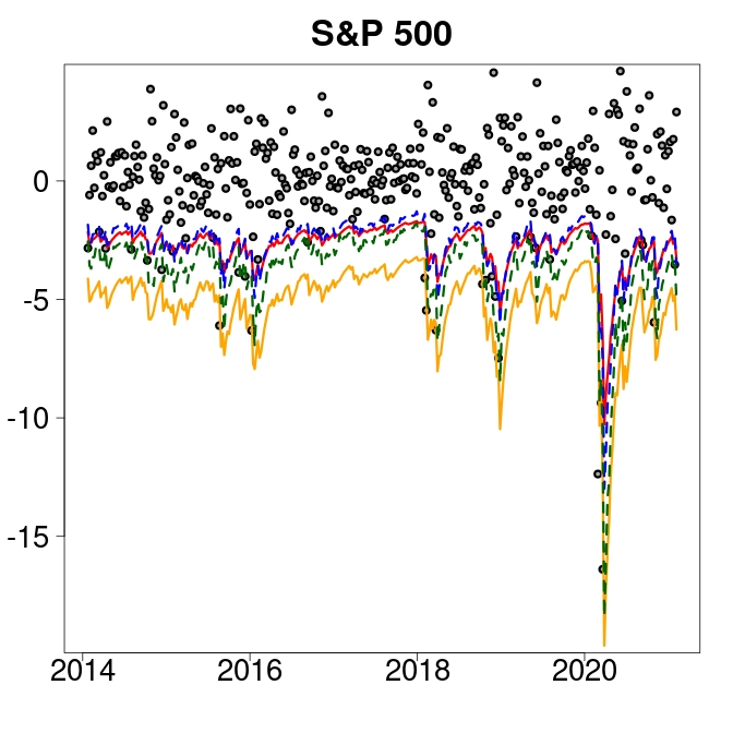
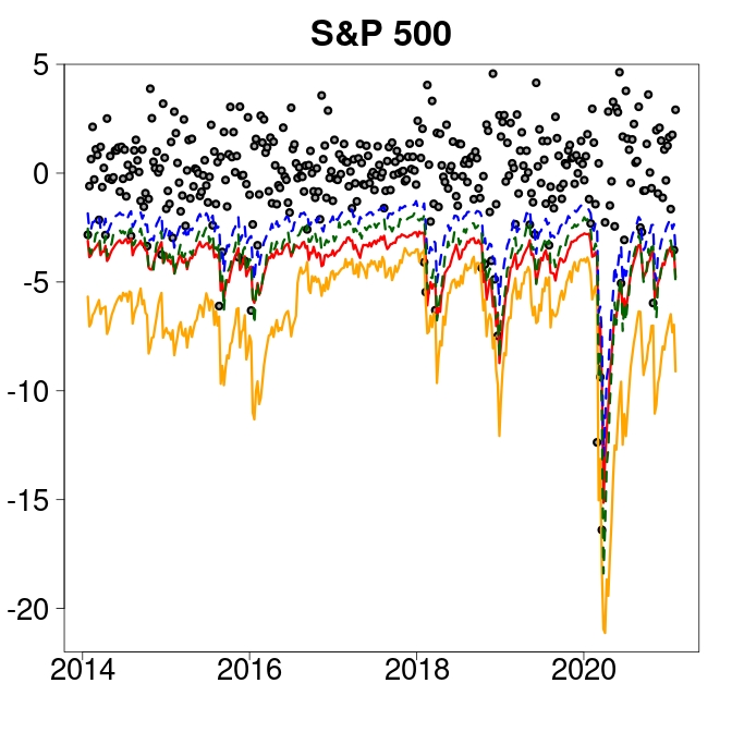
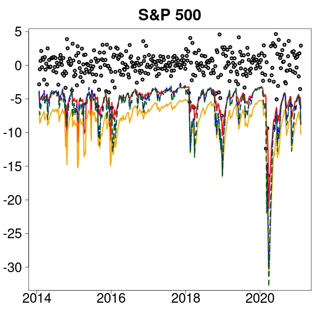
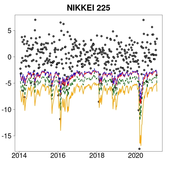
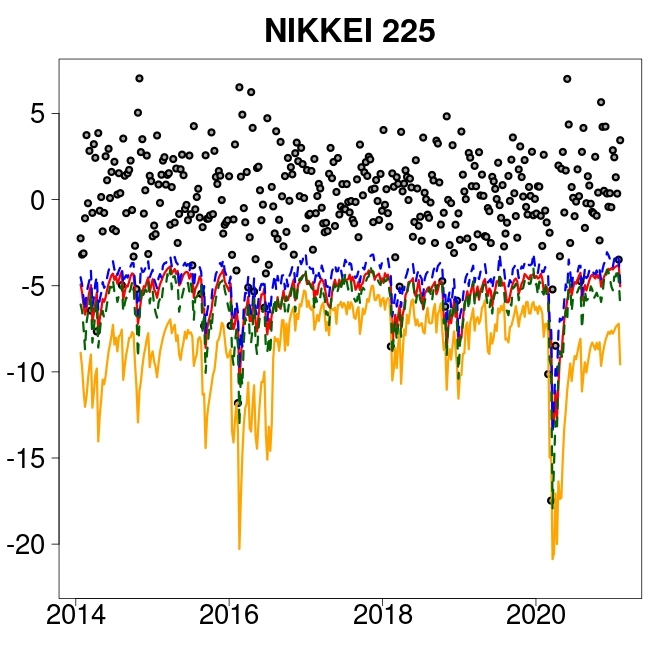
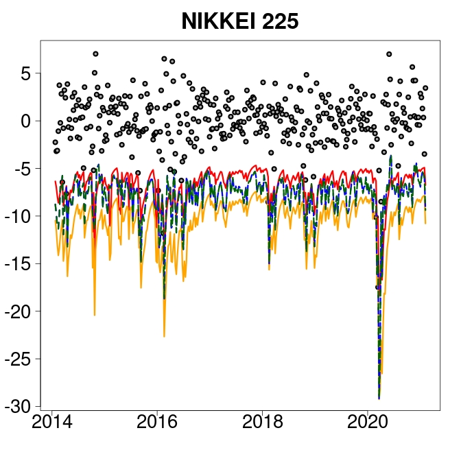
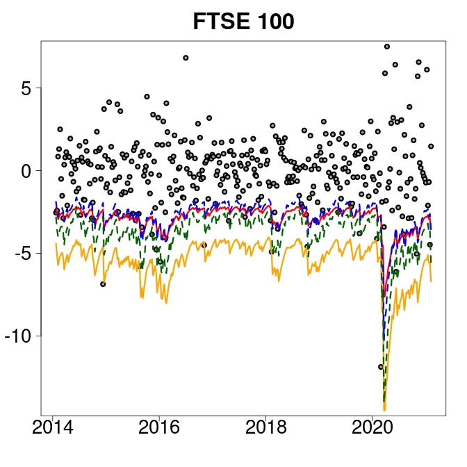
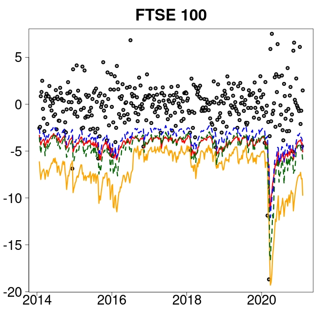
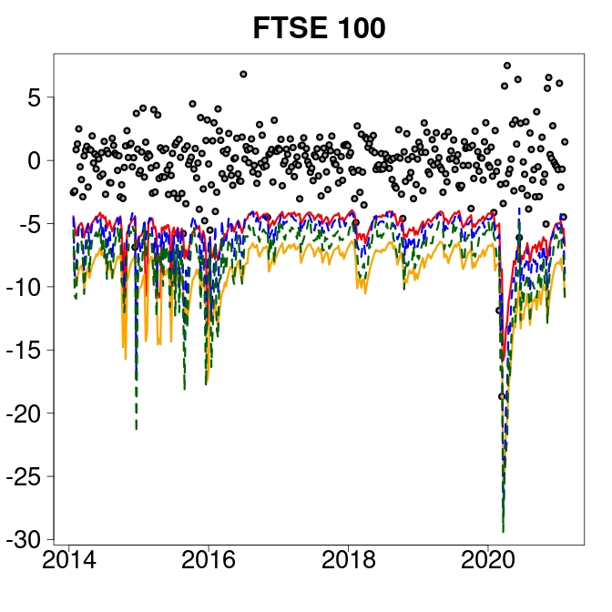
In Figure 2, we display the series of the out-of-sample forecasts of VaR and ES, for each of the three stock indices, estimated by assuming the selected CAViaR-AS specification in both the univariate and the joint approaches. VaR predictions obtained with the univariate approach of Taylor (2019) are represented by the dotted blue line, while the VaR estimates produced by our joint approach are depicted in the solid red line. The estimated ES is represented by the dotted green line (using the univariate approach) and the solid orange line (using the joint approach). Left panels of Figure 2 refer to $\boldsymbol{\tau}=[0.1,0.1,0.1]$, the center panels report the case $\boldsymbol{\tau}=[0.05,0.05,0.05]$ while the right ones consider $\boldsymbol{\tau}=[0.01,0.01,0.01]$. The gray dots denote the original return series of each stock index. In all the cases, the estimates of VaR and ES produced by our joint approach lie below the corresponding values obtained with the univariate setting, suggesting that our proposed method could lead to more conservative results.

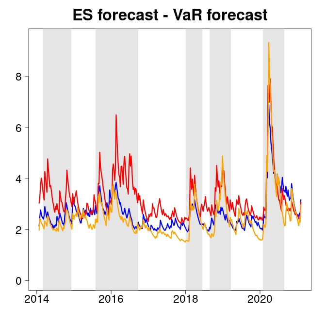
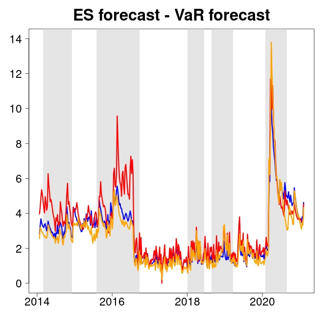
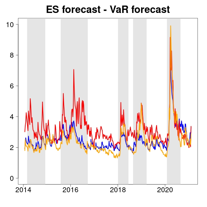
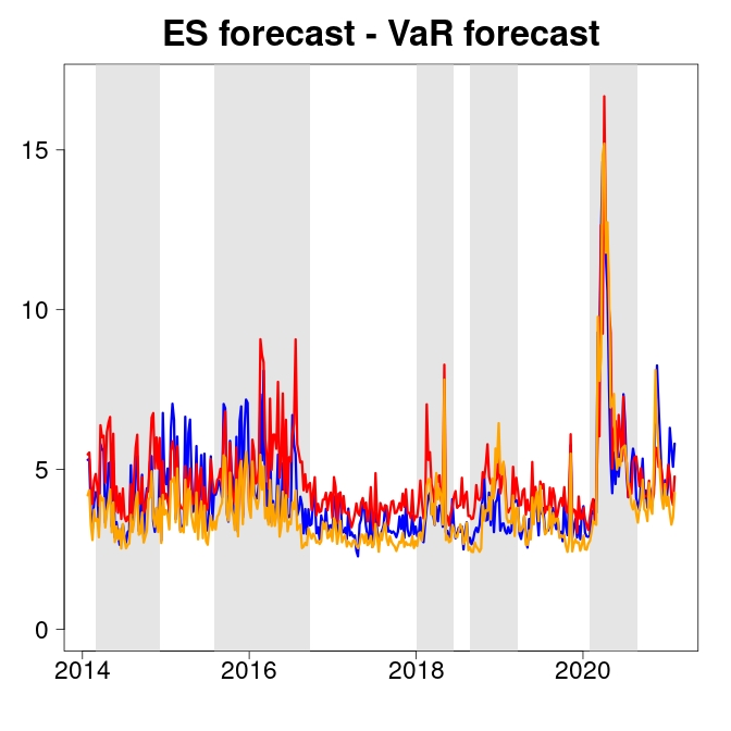
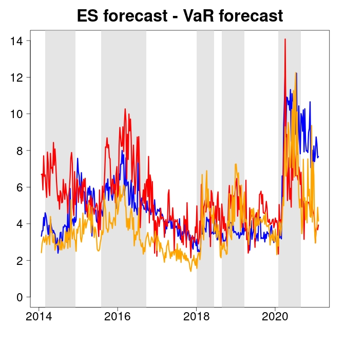
Finally, to get a more intuitive representation of the relationship between the estimated VaR and the ES over time and across the quantile levels, Figure 3 displays the absolute difference between the out-of-sample VaR and ES forecasts for each of the three stock indices. The plots in the first row are obtained by assuming the CAViaR-AS specification with the ES modeled as in (10), while the plots in the second row refer to the case of the CAViaR-AS specification with the ES following the dynamic in (11)-(12), at the $\boldsymbol{\tau}=[0.1,0.1,0.1]$ (left column), $\boldsymbol{\tau}=[0.05,0.05,0.05]$ (center column) and $\boldsymbol{\tau}=[0.01,0.01,0.01]$ (right column) quantile levels. The blue, red and orange lines refer to the FTSE 100, NIKKEI 225 and S&P 500 stock market indices, respectively, while the grey bands correspond to the main recession periods and to various economic and financial crises occurred since 2014. As one could reasonably expect, such difference follows the overall market volatility. Indeed, we find that the difference between the estimated risk measures is typically smaller in calm periods and larger in period of turbulent markets, with more pronounced upward spikes when the AR dynamics for the ES is used. High volatility is also clearly evident in correspondence and in the aftermath of major economic and financial crises, such as, for example, the Chinese stock market crash at the start of 2016, the Brexit in 2018 and the outbreak of COVID-19 pandemic in 2020.

Based on these considerations, in the next section we consider the CAViaR-AS specification in (LABEL:AS) with the ES expressed as in (10), to implement the portfolio optimization procedure.

5.3 Out-of-sample portfolio VaR and ES forecasting

In this section we use the three stock market indices of FTSE 100, NIKKEI 225 and S&P 500 to build a SMV portfolio that delivers a certain fixed level of risk $\tilde{\tau}$. The optimal allocation weights are determined by solving the optimization problem described in Section 3.2, using the parameter estimates provided by the CAViaR-AS specification in Section 5.2.

We evaluate the benefits of our approach by considering alternative strategies. First, we use the estimation method of Zhao et al. (2015), where the covariance matrix $\boldsymbol{\tilde{\Sigma}}$ in (27a) is estimated using the sample variance and the sample mean of the return series. We call this strategy Moment-SMV. Second, we evaluate the classic MV of Markowitz (1952). In this case, we model the conditional covariance of asset returns using several well-known autoregressive dynamics, i.e. the multivariate GARCH Dynamic Conditional Correlation model (Engle 2002), under both the multivariate Normal (MV-G-DCC-N) and Student-t (MV-G-DCC-t) error distributions, and the asymmetric Dynamic Conditional Correlation model with multivariate Normal (MV-G-aDCC-N) and Student-t (MV-G-aDCC-t) errors. Moreover, since the MV strategy could often be inadequate in controlling for asymmetric risk-averse agents, we also consider the above strategies under the multivariate skew Normal (SN) and the multivariate skew Student-t (St) distributions of Bauwens and Laurent (2005) as further competing strategies, which we denote by MV-G-DCC-SN, MV-G-DCC-St, MV-G-aDCC-SN and MV-G-aDCC-St, respectively. Then, for each model we forecast the one-week-ahead conditional covariance matrix and plug it into the portfolio optimization problem.

We jointly estimate VaR and ES of the resulting portfolios and analyze their out-of-sample performance using the last 368 returns of the sample. The backtesting results for the considered strategies are shown in Table 8, where we report the AL log-score of Taylor (2019), together with the S_FZN and S_FZ0 loss functions in (29) and (30) for the joint evaluation of the pair (VaR, ES). The results clearly make our approach stand out compared to the other strategies. Indeed, the strategies based on the multivariate Normal and t- distributions, and their skewed counterparts, produce highly volatile VaR forecasts and suffer from larger average losses over the out-of-sample period. On the other hand, the SMV and Moment-SMV models deliver better performance gains over the MV portfolios, with the SMV being preferred at the three VaR levels, especially at the most extreme case of $\tau=0.01$. Such gain may be traced back to the higher efficiency in the estimation procedure based on the ML approach proposed in Section 2.3. It is worth noticing that these conclusions remain still valid even when we use the $S_{FZ0}$ and the $S_{FZN}$ scoring rules, which do not directly depend on the AL likelihood function.

From a financial viewpoint, in Table 8 we also evaluate the risk-adjusted returns of the competing portfolios, measured by the Sharpe Ratio (SR) and the Herfindahl-Hirchman Index of weights concentration (HHI). We find that the SMV strategy delivers the portfolio with the highest SR and the least concentrated portfolios at both $\tau=0.1$ and $\tau=0.05$, with an average HHI of $0.558$ and $0.557$, respectively. On the other hand, when $\tau=0.01$, the MV strategy seems to yield the portfolios with the highest SR, while the Mom-SMV strategy produces the lowest degree of weights concentration.

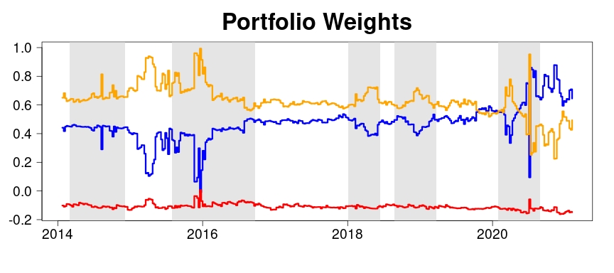
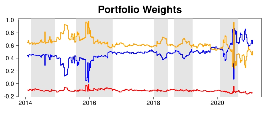
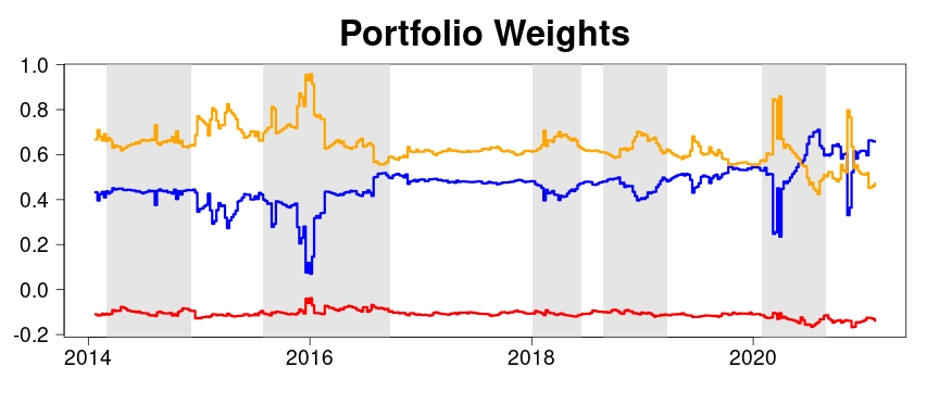
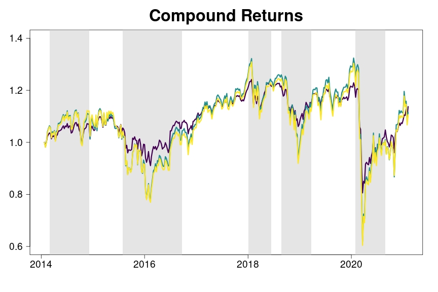
A graphical representation of the SMV portfolio weights and their evolution over time is provided in Figure 4. In each plot of the figure, the blue line denotes the allocation weights assigned to the FTSE 100, the red line refers to the NIKKEI 225, while the allocation weights of the S&P 500 are displayed in orange. The left panel considers $\tau=0.1$, the center one $\tau=0.05$, while in the right-hand side we plot the results for $\tau=0.01$. As one can see, the SMV strategy tends to invest mainly in the FTSE 100 and in the S&P 500, while it always tends to hold only a small short position on the NIKKEI 225. It is also interesting to notice that the portfolio weights exhibit the highest volatility in periods of high uncertainty in the market, such as, for example at the end of 2016 and during the ongoing COVID-19 pandemic. Finally, we evaluate the evolution of the wealth generated by the portfolios at the three risk levels during the out-of-sample period. Figure 5 highlights a positive trend for all quantile levels $\tau=0.1$ (violet line), $\tau=0.05$ (green line) and $\tau=0.01$ (yellow line) from 2014 to 2015 and from 2016 until the outbreak of COVID-19 at the beginning of 2020.

6 Discussion and conclusions

This paper proposes a dynamic joint quantile regression model for estimating VaR and ES of multiple financial assets in one step, extending the univariate framework of Taylor (2019). To implement the methodology, we suggest a likelihood-based approach based on the MAL density proposed in Petrella and Raponi (2019), generalized to the case of time-varying parameters. This offers a powerful tool to model the dynamics of multiple VaR and ES jointly. Indeed, the location parameter of the MAL density represents the vector of VaRs, while the ES can be expressed as a simple function of the density scale parameter.

We show that our approach can offer several important advantages, both theoretical and practical. First, it provides a significant gain in terms of estimation efficiency, as it allows us to estimate multiple VaR and ES in just one step. Second, it can significantly improve forecasts accuracy, since it accounts for the dependence structure among financial assets, that cannot be detected by univariate methods. These results are also confirmed empirically. Indeed, using three stock market indices as in Taylor (2019), we estimate the pairs of (VaR, ES) for each of the three assets and evaluate the forecasts using a new scoring function based on the MAL density, which allows us to account for the dependence structure among the considered assets at each point in time. The forecasts of VaR and ES have been compared with the ones obtained by the univariate approach of Taylor (2019), i.e. by considering the three stock market indices separately, as they were independent to each other. What we find is a significant gain in terms of forecasting accuracy using the proposed multivariate framework, leading to more reliable risk measure estimates.

Following Zhao et al. (2015), we also exploit the properties of the time-varying MAL distribution to derive a new portfolio optimization method, where the optimal allocation weights are adjusted at each holding period to ensure that the portfolio meets a predetermined level of risk. Empirically, we find that our optimization method produces a portfolio with less concentrated allocation weights and higher Sharpe Ratio compared to other existing strategies.

Several extensions and generalizations could be analyzed, leaving space for future research. Although we have only focused on CAViaR models, one could consider other VaR based models in the quantile regression framework and/or specify different ES dynamics where the factor $(1+e^{\gamma_{tj}})$ varies over time according to an autoregressive process for $\gamma_{tj}$. Another interesting research problem would involve the evaluation of the portfolio performance when a larger set of indices is considered, which may help us in providing an empirical ranking based on their VaR and ES forecasts. In this case, a penalized approach, as done, for instance, by Petrella and Raponi (2019), could be adopted to deal with the curse of dimensionality, improve estimation, gain in parsimony and conduct a variable selection procedure. Finally, other portfolio strategies can be implemented as well, where the choice of the weights might be motivated by other practical considerations or regulatory restrictions.

Appendix A. Proof of Proposition 1

As stated in Petrella and Raponi (2019), the $\mbox{MAL}_{p}(\boldsymbol{\mu},\boldsymbol{D}\boldsymbol{\tilde{\xi}},\boldsymbol{D}\boldsymbol{\tilde{\Sigma}}\boldsymbol{D})$ in (2.1) can be written as a location-scale mixture, having the following representation:

$$\boldsymbol{Y}=\boldsymbol{\mu}+\boldsymbol{D}\boldsymbol{\tilde{\xi}}W+\sqrt{W}\boldsymbol{D}\boldsymbol{\tilde{\Sigma}}^{1/2}\boldsymbol{Z}$$ (33)

where $\boldsymbol{\tilde{\xi}}=[\tilde{\xi}_{1},\tilde{\xi}_{2},...,\tilde{\xi}_{p}]^{\prime}$, having generic element $\tilde{\xi}_{j}=\frac{1-2\tau_{j}}{\tau_{j}(1-\tau_{j})}$, $j=1,...,p$. $\boldsymbol{\tilde{\Sigma}}$ is a $p\times p$ positive definite matrix such that $\boldsymbol{\tilde{\Sigma}}=\boldsymbol{\tilde{\Lambda}}\boldsymbol{\Psi}\boldsymbol{\tilde{\Lambda}}$, with $\boldsymbol{\Psi}$ being a correlation matrix and $\boldsymbol{\tilde{\Lambda}}=\mbox{diag}[\tilde{\sigma}_{1},\tilde{\sigma}_{1},...,\tilde{\sigma}_{p}]$, with $\tilde{\sigma}_{j}^{2}=\frac{2}{\tau_{j}(1-\tau_{j})}$, $j=1,...,p$. Finally, $\boldsymbol{Z}\sim{\cal N}_{p}(\boldsymbol{0}_{p},\boldsymbol{I}_{p})$ denotes a $p$-variate standard Normal distribution and $W\sim\mbox{Exp}(1)$ has a standard Exponential distribution, with $\boldsymbol{Z}$ being independent of $W$. Notice that, under the constraints imposed on $\boldsymbol{\tilde{\xi}}$ and $\boldsymbol{\tilde{\Lambda}}$, the representation in (33) implies that:

$$\boldsymbol{Y}\mid W=w\sim{\cal N}_{p}(\boldsymbol{\mu}+\boldsymbol{D}\boldsymbol{\tilde{\xi}}w,w\boldsymbol{D\tilde{\Sigma}D}).$$ (34)

Let $\phi_{\boldsymbol{Y}}(\boldsymbol{t})$ denote the characteristic function of $\boldsymbol{Y}$, with $\boldsymbol{t}\in{\cal R}^{p}$. Using the result in (33), it follows that:

$$\phi_{\boldsymbol{Y}}(\boldsymbol{t})=\mathbb{E}_{W}\left[\mathbb{E}_{Y}[e^{i\boldsymbol{t^{\prime}Y}}\mid W=w]\right]=\int_{0}^{\infty}\mathbb{E}_{Z}[e^{i\boldsymbol{t^{\prime}}(\boldsymbol{\mu}+\boldsymbol{D\tilde{\xi}}w+\sqrt{w}\boldsymbol{D\tilde{\Sigma}}^{\frac{1}{2}}\boldsymbol{Z})}\mid W=w]e^{-w}dw.$$ (35)

Now, using the conditional distribution of $\boldsymbol{Y}$ given $W$ in (34), we have that:

$$\mathbb{E}_{Z}[e^{i\boldsymbol{t^{\prime}}(\boldsymbol{\mu}+\boldsymbol{D\tilde{\xi}}w+\sqrt{w}\boldsymbol{D\tilde{\Sigma}}^{\frac{1}{2}}\boldsymbol{Z})}\mid W=w]=e^{i\boldsymbol{t^{\prime}\mu}+i\boldsymbol{t^{\prime}D\tilde{\xi}}w-\frac{w}{2}\boldsymbol{t^{\prime}D\tilde{\Sigma}Dt}}.$$

Substituting this result into (35) yields:

$$\phi_{\boldsymbol{Y}}(\boldsymbol{t}) = e^{i\boldsymbol{t^{\prime}\mu}}\int_{0}^{\infty}e^{-w(1+\frac{1}{2}\boldsymbol{t^{\prime}D\tilde{\Sigma}Dt}-i\boldsymbol{t^{\prime}D\tilde{\xi}})}dw.$$ (36)

Finally, integrating over $W$, we obtain:

$$\phi_{\boldsymbol{Y}}(\boldsymbol{t}) = e^{i\boldsymbol{t^{\prime}\mu}}\left(1+\frac{1}{2}\boldsymbol{t^{\prime}D\tilde{\Sigma}Dt}-i\boldsymbol{t^{\prime}D\tilde{\xi}}\right)^{-1}.$$ (37)

Now, let $\boldsymbol{b}=(b_{1},...,b_{p})^{\prime}\in{\cal R}^{p}$ be a $p\times 1$ vector such that $\boldsymbol{b}\neq\boldsymbol{0}_{p}$ and consider a new random variable $Y^{\boldsymbol{b}}=\sum_{j=1}^{p}b_{j}Y_{j}={\boldsymbol{b}}^{\prime}{\boldsymbol{Y}}$, having characteristic function $\phi_{Y^{\boldsymbol{b}}}(z)$, with $z\in{\cal R}$. Notice that $Y^{\boldsymbol{b}}$ is a linear transformation of the marginals $Y_{1},\dots,Y_{p}$. Therefore, the relation $\phi_{Y^{\boldsymbol{b}}}(z)=\phi_{\boldsymbol{b^{\prime}Y}}(z)=\phi_{\boldsymbol{Y}}(\boldsymbol{b}z)$ holds, since:

$$\phi_{Y^{\boldsymbol{b}}}(z) = e^{iz\boldsymbol{b^{\prime}\mu}}\left(1+\frac{1}{2}z^{2}\boldsymbol{b^{\prime}D\tilde{\Sigma}Db}-iz\boldsymbol{b^{\prime}D\tilde{\xi}}\right)^{-1}.$$ (38)

The characteristic function in (38) resembles the characteristic function of the AL univariate distribution discussed in Yu and Moyeed (2001) and Kozumi and Kobayashi (2011) where $\mu^{\star},\tau^{\star},\delta^{\star}$ are the scale, skewness and scale parameters, respectively. Therefore, the characteristic function of $Y^{\boldsymbol{b}}$ in (38) can be rewritten as the characteristic function of a univariate AL distribution with parameters:

$$\mu^{\star}=\boldsymbol{b^{\prime}\mu}\mbox{,}\quad\tau^{\star}=\frac{1}{2}\left(1-\frac{\boldsymbol{b^{\prime}D\tilde{\xi}}}{\sqrt{2(\boldsymbol{b^{\prime}D\tilde{\Sigma}Db})+(\boldsymbol{b^{\prime}D\tilde{\xi}})^{2}}}\right)\quad\mbox{and}\quad\delta^{\star}=\frac{(\boldsymbol{b^{\prime}D\tilde{\Sigma}Db})}{2{\sqrt{2(\boldsymbol{b^{\prime}D\tilde{\Sigma}Db})+(\boldsymbol{b^{\prime}D\tilde{\xi}})^{2}}}}.$$

∎

In conclusion, we obtain that $Y^{\boldsymbol{b}}\sim\mbox{AL}(\mu^{\star},\tau^{\star},\delta^{\star})$ and $\mathbb{P}(Y^{\boldsymbol{b}}<\mu^{\star})=\tau^{\star}$. Consequently, the parameter $\tau^{\star}$ controls the probability assigned to each side of $Y^{\boldsymbol{b}}$ and $\mu^{\star}$ is the corresponding quantile at level $\tau^{\star}$. Notice that the denominator $2(\boldsymbol{b^{\prime}D\tilde{\Sigma}Db})+(\boldsymbol{b^{\prime}D\tilde{\xi}})^{2}$ in (Appendix A. Proof of Proposition 1) is well defined on the positive real line since $(\boldsymbol{b^{\prime}D\tilde{\xi}})^{2}\geq 0$ and $2(\boldsymbol{b^{\prime}D\tilde{\Sigma}Db})>0$ because $\boldsymbol{\tilde{\Sigma}}$ is a positive definite matrix. Furthermore, when $\boldsymbol{\tau}=[0.5,0.5,...,0.5]$, we have that $\boldsymbol{b^{\prime}D\tilde{\xi}}=0$ and (Appendix A. Proof of Proposition 1) simplifies to $\tau^{\star}=0.5$ and $\delta^{\star}=\frac{\sqrt{\boldsymbol{b^{\prime}D\tilde{\Sigma}Db}}}{2\sqrt{2}}$, which implies that the distribution of $Y^{\boldsymbol{b}}$ is symmetric around $\mu^{\star}$.

Appendix B. Simulation study

In this Appendix we conduct a simulation study to evaluate the finite sample properties of the proposed method and its ability to jointly estimate the pair (VaR, ES) for multiple correlated assets. This simulation exercise addresses the following issues. First, we consider different distributional choices for the error term to investigate the behaviour of the model in the presence of non-Gaussian errors. Second, we evaluate the bias and accuracy of the ML estimators when the interest of the research is focused upon the lower tails of the distribution. Finally, we inspect the impact of dimensionality on both the estimated parameters and the computational burden of the optimization routine.

In the first experiment, we consider a sample size of $T=1500$ and set $p=3$. The observations are simulated using the following data generating process:

$$\boldsymbol{Y}_{t}={\cal Q}_{\boldsymbol{Y}_{t}}(\boldsymbol{\tau}|\mathcal{F}_{t-1})+\boldsymbol{\epsilon}_{t},\quad\quad t=1,2,...,T,$$ (40)

where ${\cal Q}_{\boldsymbol{Y}_{t}}(\boldsymbol{\tau}|\mathcal{F}_{t-1})$ is generated according to the three different CAViaR specifications described in (LABEL:SAV)-(LABEL:IG). For the ES component we adopted both the multiplicative factor specification in (10) and the AR formulation in (11)-(12). Following Petrella and Raponi (2019), two different simulation scenarios are considered for the error terms $\boldsymbol{\epsilon}_{t}$ in (40):

1. (i) a multivariate Normal distribution ($\mathcal{N}_{3})$ with zero mean and variance-covariance matrix equal to $\boldsymbol{D}_{t}\boldsymbol{\tilde{\Sigma}}\boldsymbol{D}_{t}$, that is $\boldsymbol{\epsilon}_{it}\sim\mathcal{N}_{3}(\boldsymbol{0},\boldsymbol{D}_{t}\boldsymbol{\tilde{\Sigma}}\boldsymbol{D}_{t})$;

2. (ii) a multivariate Student-t distribution ($\mathcal{T}_{3}$) with 5 degrees of freedom, scale parameter $\boldsymbol{D}_{t}\boldsymbol{\tilde{\Sigma}}\boldsymbol{D}_{t}$ and non centrality parameter equal to $\boldsymbol{D}_{t}\boldsymbol{\tilde{\xi}}$, that is $\boldsymbol{\epsilon}_{it}\sim\mathcal{T}_{3}(5,\boldsymbol{D}_{t}\boldsymbol{\tilde{\xi}},\boldsymbol{D}_{t}\boldsymbol{\tilde{\Sigma}}\boldsymbol{D}_{t})$.

The true values of the CAViaR model and the ES dynamics are calibrated using the real data in the empirical application. Specifically, we set

$$\boldsymbol{\omega}=[-0.20,-0.12,-0.24]^{\prime},\quad\boldsymbol{\eta}=[0.85,0.70,0.60]^{\prime},\quad\boldsymbol{\beta}_{1}=[-0.10,-0.05,-0.20]^{\prime},\quad\boldsymbol{\beta}_{2}=[0.05,0.10,0.20]^{\prime}$$

and

$$\boldsymbol{\gamma}_{0}=[-1.1,-1.5,-1.3]^{\prime},\quad\boldsymbol{\gamma}_{1}=[0.05,0.10,0.02]^{\prime},\quad\boldsymbol{\gamma}_{2}=[0.12,0.05,0.20]^{\prime}\quad\textnormal{and}\quad\boldsymbol{\gamma}_{3}=[0.80,0.70,0.60]^{\prime}.$$

For the CAViaR-IG dynamic, each element of the vector $\boldsymbol{\omega}$ is considered in absolute value to guarantee that the autoregressive process in (LABEL:IG) is well-defined. Finally, we set $\boldsymbol{\Psi}=\begin{bmatrix}1&0.3&0.7\\ 0.3&1&0.5\\ 0.7&0.5&1\end{bmatrix}$.
Since we are interested in evaluating the downside risk, we analyze three different quantile vectors, namely $\boldsymbol{\tau}=[0.1,0.1,0.1]$, $\boldsymbol{\tau}=[0.05,0.05,0.05]$ and $\boldsymbol{\tau}=[0.01,0.01,0.01]$. For each model, we carry out $B=250$ Monte Carlo replications and report the percentage relative bias (Bias%) and the Root Mean Square Error (RMSE), averaged across the B simulations. Tables 9 and 10 report the results for all the parameters $\boldsymbol{\omega},\boldsymbol{\eta}$ and $\boldsymbol{\beta}$ of the three CAViaR specifications. As can be noted, our estimation method is able to recover the true CAViaR specifications under both the $\mathcal{N}_{3}$- and $\mathcal{T}_{3}$- scenarios, and for both the considered ES dynamics. Indeed, both the Bias% and the RMSE remain reasonably small under all the different scenarios even though, as expected, their values tend to slightly increase as the quantile level becomes more extreme (due to the reduced information available at the tails of the distribution) and when we consider a heavy-tailed distribution ($\mathcal{T}_{3}$-scenario). To computationally evaluate the speed of convergence of the EM algorithm, in the last row of each panel we also report the median number of iterations and CPU Time (in seconds) required by the implemented R code using an Intel Xeon E5-2609 2.40GHz processor. Running times range from $9.613$ seconds for the simplest SAV specification with a constant multiplicative factor specified for the ES component, up to $47.242$ seconds for the most complex AS model with autoregressive ES component, confirming the practical feasibility of our optimization algorithm.

Finally, to evaluate the impact of dimensionality on the optimization routine, we considered the same simulation experiment in (40) with $T=1500$ and $\boldsymbol{\tau}=[0.1,0.1,...,0.1]$, and let $p=\{3,5,10,12\}$ grow. Specifically, for each value of $p$, Tables 11 and 12 report the Bias% and RMSE of the parameter $\theta=\mid\mid\boldsymbol{\theta}\mid\mid$ over 100 Monte Carlo replications, where $\boldsymbol{\theta}=[\boldsymbol{\omega},\boldsymbol{\eta},\boldsymbol{\beta}]^{\prime}$ and $\mid\mid\cdot\mid\mid$ denote the $\ell_{1}$ norm of $\boldsymbol{\theta}$. As before, we also report the median number of iterations and CPU Time (in seconds) needed to fit the model. As one can easily see, the Bias% remains relatively constant regardless of the value of $p$, even though, as expected, the RMSE slightly increases with the dimensionality of the problem.

CAViaR	SAV			AS			IG
$\boldsymbol{\tau}$	$[0.1,0.1,0.1]$	$[0.05,0.05,0.05]$	$[0.01,0.01,0.01]$	$[0.1,0.1,0.1]$	$[0.05,0.05,0.05]$	$[0.01,0.01,0.01]$	$[0.1,0.1,0.1]$	$[0.05,0.05,0.05]$	$[0.01,0.01,0.01]$
Panel A: $\boldsymbol{\epsilon}_{it}\sim\mathcal{N}_{3}(\boldsymbol{0},\boldsymbol{D}_{t}\boldsymbol{\tilde{\Sigma}}\boldsymbol{D}_{t})$
$\omega_{1}$	$-0.120\;(0.027)$	$0.758\;(0.047)$	$3.874\;(0.149)$	$-1.621\;(0.036)$	$-2.048\;(0.050)$	$-3.472\;(0.151)$	$-1.494\;(0.031)$	$2.520\;(0.044)$	$3.749\;(0.156)$
$\omega_{2}$	$-1.020\;(0.037)$	$-3.119\;(0.052)$	$2.057\;(0.145)$	$-1.265\;(0.030)$	$-3.738\;(0.054)$	$-4.086\;(0.169)$	$-1.334\;(0.036)$	$1.558\;(0.053)$	$3.622\;(0.142)$
$\omega_{3}$	$-1.371\;(0.028)$	$-2.245\;(0.053)$	$3.900\;(0.162)$	$-1.454\;(0.035)$	$-2.617\;(0.063)$	$-3.238\;(0.147)$	$-1.195\;(0.033)$	$2.751\;(0.048)$	$3.964\;(0.148)$
$\eta_{1}$	$1.184\;(0.025)$	$1.337\;(0.057)$	$-1.528\;(0.153)$	$2.241\;(0.030)$	$2.379\;(0.049)$	$-3.185\;(0.155)$	$0.548\;(0.048)$	$-2.690\;(0.059)$	$-2.941\;(0.159)$
$\eta_{2}$	$1.228\;(0.035)$	$1.753\;(0.041)$	$-2.537\;(0.143)$	$-0.179\;(0.034)$	$-1.855\;(0.062)$	$1.992\;(0.199)$	$1.794\;(0.039)$	$-2.314\;(0.041)$	$-3.570\;(0.144)$
$\eta_{3}$	$1.560\;(0.027)$	$2.472\;(0.036)$	$-1.132\;(0.174)$	$1.830\;(0.041)$	$2.991\;(0.062)$	$4.230\;(0.178)$	$1.981\;(0.031)$	$2.220\;(0.054)$	$2.781\;(0.153)$
$\beta_{11}$	$-1.573\;(0.031)$	$-2.688\;(0.038)$	$3.971\;(0.155)$	$-1.409\;(0.035)$	$-3.308\;(0.056)$	$-3.366\;(0.168)$	$-0.141\;(0.040)$	$2.704\;(0.041)$	$3.497\;(0.162)$
$\beta_{12}$	$-0.841\;(0.033)$	$-1.521\;(0.060)$	$2.459\;(0.140)$	$-0.517\;(0.031)$	$-0.797\;(0.045)$	$1.871\;(0.159)$	$1.427\;(0.045)$	$1.981\;(0.062)$	$2.082\;(0.185)$
$\beta_{13}$	$-1.799\;(0.045)$	$-2.066\;(0.057)$	$3.211\;(0.165)$	$-1.439\;(0.039)$	$-1.937\;(0.055)$	$3.540\;(0.167)$	$1.899\;(0.041)$	$2.853\;(0.073)$	$3.198\;(0.159)$
$\beta_{21}$				$1.862\;(0.033)$	$2.008\;(0.046)$	$5.335\;(0.147)$
$\beta_{22}$				$-0.187\;(0.039)$	$1.705\;(0.054)$	$4.059\;(0.161)$
$\beta_{23}$				$0.634\;(0.039)$	$1.089\;(0.049)$	$3.899\;(0.158)$
Iterations	6	8	12	8	14	27	6	9	14
CPU Time	9.613	11.824	17.090	11.498	22.830	33.933	9.669	12.816	18.159
Panel B: $\boldsymbol{\epsilon}_{it}\sim\mathcal{T}_{3}(5,\boldsymbol{D}_{t}\boldsymbol{\tilde{\xi}},\boldsymbol{D}_{t}\boldsymbol{\tilde{\Sigma}}\boldsymbol{D}_{t})$
$\omega_{1}$	$-1.196\;(0.039)$	$-2.393\;(0.063)$	$2.996\;(0.156)$	$-0.196\;(0.049)$	$-2.898\;(0.051)$	$-2.393\;(0.168)$	$-1.291\;(0.029)$	$1.996\;(0.056)$	$3.560\;(0.163)$
$\omega_{2}$	$-1.833\;(0.045)$	$-1.572\;(0.059)$	$1.385\;(0.162)$	$-2.833\;(0.035)$	$-2.380\;(0.052)$	$-4.572\;(0.179)$	$-1.533\;(0.034)$	$1.385\;(0.052)$	$2.608\;(0.160)$
$\omega_{3}$	$-1.397\;(0.036)$	$-1.297\;(0.041)$	$3.736\;(0.168)$	$-2.397\;(0.046)$	$-2.120\;(0.061)$	$-4.297\;(0.151)$	$-1.558\;(0.032)$	$1.736\;(0.068)$	$1.825\;(0.169)$
$\eta_{1}$	$2.699\;(0.051)$	$0.292\;(0.067)$	$-2.097\;(0.170)$	$2.699\;(0.041)$	$2.266\;(0.057)$	$2.292\;(0.167)$	$1.132\;(0.027)$	$-2.097\;(0.050)$	$-1.940\;(0.164)$
$\eta_{2}$	$1.050\;(0.048)$	$1.849\;(0.068)$	$-4.367\;(0.177)$	$0.050\;(0.038)$	$1.421\;(0.047)$	$1.849\;(0.198)$	$1.805\;(0.037)$	$-2.367\;(0.047)$	$-3.034\;(0.153)$
$\eta_{3}$	$1.508\;(0.042)$	$2.455\;(0.061)$	$3.581\;(0.167)$	$1.508\;(0.032)$	$1.783\;(0.049)$	$3.455\;(0.151)$	$1.335\;(0.036)$	$1.581\;(0.057)$	$2.243\;(0.140)$
$\beta_{11}$	$-1.718\;(0.030)$	$-0.402\;(0.050)$	$2.688\;(0.154)$	$-2.718\;(0.049)$	$-3.440\;(0.068)$	$-3.702\;(0.160)$	$-1.908\;(0.036)$	$2.688\;(0.054)$	$1.954\;(0.162)$
$\beta_{12}$	$-1.615\;(0.048)$	$-0.402\;(0.052)$	$3.189\;(0.163)$	$-1.615\;(0.038)$	$-2.691\;(0.064)$	$-2.402\;(0.147)$	$-0.940\;(0.034)$	$1.189\;(0.053)$	$2.514\;(0.189)$
$\beta_{13}$	$-2.557\;(0.037)$	$1.942\;(0.049)$	$3.087\;(0.180)$	$-2.157\;(0.047)$	$-2.542\;(0.060)$	$1.942\;(0.199)$	$1.769\;(0.041)$	$2.087\;(0.080)$	$3.941\;(0.170)$
$\beta_{21}$				$1.371\;(0.059)$	$1.057\;(0.056)$	$3.782\;(0.170)$
$\beta_{22}$				$-0.803\;(0.040)$	$-1.690\;(0.052)$	$1.166\;(0.166)$
$\beta_{23}$				$0.489\;(0.039)$	$1.607\;(0.065)$	$2.210\;(0.163)$
Iterations	7	10	15	11	16	28	7	11	16
CPU Time	9.617	12.799	18.141	11.691	22.983	34.631	9.628	13.812	18.385

Table 9: Bias% and RMSE (in brackets) of point estimates for $\boldsymbol{\omega},\boldsymbol{\eta}$ and $\boldsymbol{\beta}$ of the three CAViaR specifications in (LABEL:SAV)-(LABEL:IG) with the ES modeled as a multiple of VaR as in (10), under the $\mathcal{N}_{3}$- and $\mathcal{T}_{3}$- scenarios. The last two rows of each Panel show the median number of iterations and CPU Time (in seconds) required to fit the model using a single run of the EM algorithm.

CAViaR	SAV			AS			IG
$\boldsymbol{\tau}$	$[0.1,0.1,0.1]$	$[0.05,0.05,0.05]$	$[0.01,0.01,0.01]$	$[0.1,0.1,0.1]$	$[0.05,0.05,0.05]$	$[0.01,0.01,0.01]$	$[0.1,0.1,0.1]$	$[0.05,0.05,0.05]$	$[0.01,0.01,0.01]$
Panel A: $\boldsymbol{\epsilon}_{it}\sim\mathcal{N}_{3}(\boldsymbol{0},\boldsymbol{D}_{t}\boldsymbol{\tilde{\Sigma}}\boldsymbol{D}_{t})$
$\omega_{1}$	$-0.688\;(0.037)$	$-2.193\;(0.094)$	$-3.853\;(0.155)$	$-2.266\;(0.060)$	$2.609\;(0.156)$	$2.245\;(0.196)$	$0.505\;(0.059)$	$-2.726\;(0.075)$	$2.522\;(0.150)$
$\omega_{2}$	$-0.413\;(0.037)$	$-2.936\;(0.053)$	$-3.462\;(0.165)$	$-1.189\;(0.065)$	$2.139\;(0.055)$	$3.807\;(0.191)$	$-1.986\;(0.077)$	$-2.309\;(0.084)$	$3.130\;(0.162)$
$\omega_{3}$	$-1.796\;(0.055)$	$-1.046\;(0.063)$	$-3.785\;(0.145)$	$-1.949\;(0.057)$	$1.749\;(0.073)$	$2.424\;(0.165)$	$-1.162\;(0.064)$	$-4.810\;(0.121)$	$3.644\;(0.153)$
$\eta_{1}$	$1.691\;(0.037)$	$2.940\;(0.061)$	$2.999\;(0.140)$	$0.642\;(0.061)$	$-3.533\;(0.067)$	$-2.804\;(0.199)$	$1.430\;(0.040)$	$-2.116\;(0.074)$	$-3.672\;(0.162)$
$\eta_{2}$	$1.884\;(0.043)$	$-2.023\;(0.050)$	$-2.133\;(0.177)$	$-1.217\;(0.052)$	$-2.763\;(0.091)$	$-4.777\;(0.140)$	$-1.813\;(0.054)$	$-1.854\;(0.119)$	$-3.088\;(0.155)$
$\eta_{3}$	$1.018\;(0.065)$	$-1.174\;(0.057)$	$3.017\;(0.162)$	$-3.500\;(0.065)$	$-2.376\;(0.045)$	$-2.197\;(0.150)$	$1.158\;(0.081)$	$-2.133\;(0.136)$	$-2.316\;(0.167)$
$\beta_{11}$	$-1.850\;(0.048)$	$-3.514\;(0.045)$	$3.345\;(0.133)$	$1.850\;(0.064)$	$1.395\;(0.053)$	$4.856\;(0.176)$	$-2.688\;(0.060)$	$1.699\;(0.102)$	$2.803\;(0.189)$
$\beta_{12}$	$-1.609\;(0.041)$	$-2.701\;(0.057)$	$2.465\;(0.186)$	$2.602\;(0.066)$	$3.041\;(0.091)$	$3.230\;(0.141)$	$-2.357\;(0.074)$	$-2.640\;(0.128)$	$2.921\;(0.182)$
$\beta_{13}$	$-1.224\;(0.038)$	$-1.291\;(0.045)$	$2.808\;(0.164)$	$1.659\;(0.063)$	$2.407\;(0.067)$	$4.289\;(0.119)$	$-1.928\;(0.065)$	$-2.191\;(0.117)$	$4.053\;(0.143)$
$\beta_{21}$				$1.320\;(0.058)$	$-2.763\;(0.141)$	$-2.013\;(0.193)$
$\beta_{22}$				$1.599\;(0.069)$	$-2.484\;(0.121)$	$-3.276\;(0.162)$
$\beta_{23}$				$1.082\;(0.060)$	$-2.179\;(0.118)$	$3.936\;(0.174)$
Iterations	12	14	19	15	23	35	10	15	18
CPU Time	13.791	20.739	25.738	16.112	22.956	45.946	13.796	20.781	25.784
Panel B: $\boldsymbol{\epsilon}_{it}\sim\mathcal{T}_{3}(5,\boldsymbol{D}_{t}\boldsymbol{\tilde{\xi}},\boldsymbol{D}_{t}\boldsymbol{\tilde{\Sigma}}\boldsymbol{D}_{t})$
$\omega_{1}$	$-1.687\;(0.049)$	$-3.265\;(0.121)$	$-3.792\;(0.151)$	$-2.793\;(0.037)$	$2.309\;(0.126)$	$3.497\;(0.215)$	$-1.006\;(0.038)$	$-2.278\;(0.117)$	$3.580\;(0.142)$
$\omega_{2}$	$-2.891\;(0.078)$	$-2.992\;(0.084)$	$-4.143\;(0.189)$	$-1.244\;(0.048)$	$4.041\;(0.121)$	$4.667\;(0.223)$	$-2.308\;(0.069)$	$-3.344\;(0.102)$	$2.875\;(0.127)$
$\omega_{3}$	$-1.169\;(0.087)$	$-2.719\;(0.128)$	$-4.852\;(0.156)$	$-1.529\;(0.070)$	$1.858\;(0.093)$	$2.045\;(0.216)$	$-1.845\;(0.044)$	$-2.442\;(0.125)$	$4.644\;(0.194)$
$\eta_{1}$	$2.834\;(0.038)$	$3.721\;(0.096)$	$-3.089\;(0.157)$	$1.081\;(0.057)$	$2.490\;(0.171)$	$-3.874\;(0.190)$	$1.595\;(0.051)$	$2.387\;(0.093)$	$-4.524\;(0.146)$
$\eta_{2}$	$-1.345\;(0.062)$	$-2.788\;(0.166)$	$-4.423\;(0.154)$	$-1.449\;(0.063)$	$-2.036\;(0.176)$	$-3.810\;(0.215)$	$0.404\;(0.059)$	$-2.002\;(0.086)$	$-4.258\;(0.189)$
$\eta_{3}$	$1.642\;(0.067)$	$-2.089\;(0.094)$	$-2.026\;(0.144)$	$-1.104\;(0.073)$	$2.716\;(0.096)$	$-2.981\;(0.221)$	$2.186\;(0.057)$	$3.929\;(0.106)$	$2.565\;(0.192)$
$\beta_{11}$	$-2.171\;(0.046)$	$-3.313\;(0.091)$	$2.090\;(0.132)$	$0.920\;(0.066)$	$3.032\;(0.133)$	$3.917\;(0.186)$	$-1.893\;(0.040)$	$-3.994\;(0.138)$	$3.613\;(0.161)$
$\beta_{12}$	$-2.212\;(0.050)$	$-3.605\;(0.112)$	$1.394\;(0.146)$	$1.261\;(0.082)$	$2.959\;(0.090)$	$3.883\;(0.197)$	$-1.525\;(0.047)$	$-2.143\;(0.104)$	$3.346\;(0.181)$
$\beta_{13}$	$-1.536\;(0.042)$	$-2.111\;(0.085)$	$3.773\;(0.129)$	$1.971\;(0.082)$	$3.189\;(0.145)$	$2.862\;(0.184)$	$-2.807\;(0.054)$	$-3.592\;(0.092)$	$4.842\;(0.164)$
$\beta_{21}$				$1.171\;(0.051)$	$1.847\;(0.137)$	$3.866\;(0.177)$
$\beta_{22}$				$1.229\;(0.067)$	$2.621\;(0.154)$	$3.195\;(0.196)$
$\beta_{23}$				$1.456\;(0.063)$	$2.158\;(0.133)$	$3.535\;(0.187)$
Iterations	13	14	20	16	24	37	11	16	20
CPU Time	13.797	20.760	25.790	16.783	22.176	47.242	13.794	20.752	26.766

Table 10: Bias% and RMSE (in brackets) of point estimates for $\boldsymbol{\omega},\boldsymbol{\eta}$ and $\boldsymbol{\beta}$ of the three CAViaR specifications in (LABEL:SAV)-(LABEL:IG) with the AR process for the ES as in (11)-(12), under the $\mathcal{N}_{3}$- and $\mathcal{T}_{3}$- scenarios. The last two rows of each Panel show the median number of iterations and CPU Time (in seconds) required to fit the model using a single run of the EM algorithm.

	$p=3$			$p=5$			$p=10$			$p=12$
CAViaR	SAV	AS	IG	SAV	AS	IG	SAV	AS	IG	SAV	AS	IG
Panel A: $\boldsymbol{\epsilon}_{it}\sim\mathcal{N}_{3}(\boldsymbol{0},\boldsymbol{D}_{t}\boldsymbol{\tilde{\Sigma}}\boldsymbol{D}_{t})$
Bias%	0.754	0.672	0.855	0.697	0.742	0.748	0.803	0.729	0.764	0.869	0.680	0.654
RMSE	0.083	0.088	0.075	0.118	0.390	0.272	0.299	0.267	0.315	0.351	0.391	0.341
Iterations	6	9	6	12	14	11	18	27	22	47	55	48
CPU Time	9.812	11.746	9.756	46.207	60.240	47.248	88.980	102.840	98.040	126.540	137.880	120.660
Panel B: $\boldsymbol{\epsilon}_{it}\sim\mathcal{T}_{3}(5,\boldsymbol{D}_{t}\boldsymbol{\tilde{\xi}},\boldsymbol{D}_{t}\boldsymbol{\tilde{\Sigma}}\boldsymbol{D}_{t})$
Bias%	0.837	0.809	0.785	0.793	0.884	0.895	0.734	0.831	0.702	0.893	0.708	0.929
RMSE	0.095	0.085	0.083	0.207	0.375	0.321	0.372	0.396	0.380	0.362	0.379	0.442
Iterations	6	9	7	11	16	12	18	29	23	48	57	50
CPU Time	9.783	11.742	9.776	47.900	64.440	48.944	84.720	98.840	96.760	130.200	164.100	155.460

Table 11: Bias% and RMSE of point estimates of $\theta=\mid\mid\boldsymbol{\theta}\mid\mid$, where $\boldsymbol{\theta}=[\boldsymbol{\omega},\boldsymbol{\eta},\boldsymbol{\beta}]^{\prime}$, for different values of $p$ and for the three CAViaR specifications in (LABEL:SAV)-(LABEL:IG), with the ES modeled as a multiple of VaR as in (10). Panels A and B refer to the $\mathcal{N}_{3}$- and $\mathcal{T}_{3}$- scenarios, respectively, where the last two rows of each panel show the median number of iterations and CPU Time (in seconds) required to fit the model using a single run of the EM algorithm.

	$p=3$			$p=5$			$p=10$			$p=12$
CAViaR	SAV	AS	IG	SAV	AS	IG	SAV	AS	IG	SAV	AS	IG
Panel A: $\boldsymbol{\epsilon}_{it}\sim\mathcal{N}_{3}(\boldsymbol{0},\boldsymbol{D}_{t}\boldsymbol{\tilde{\Sigma}}\boldsymbol{D}_{t})$
Bias%	0.786	0.791	0.773	0.731	0.865	0.671	0.912	0.713	0.792	0.803	0.753	0.800
RMSE	0.140	0.149	0.147	0.265	0.279	0.232	0.243	0.322	0.223	0.364	0.358	0.437
Iterations	12	13	11	23	24	21	38	37	35	67	75	68
CPU Time	12.617	15.799	13.141	82.140	89.400	85.400	109.680	168.240	118.320	196.620	303.360	196.540
Panel B: $\boldsymbol{\epsilon}_{it}\sim\mathcal{T}_{3}(5,\boldsymbol{D}_{t}\boldsymbol{\tilde{\xi}},\boldsymbol{D}_{t}\boldsymbol{\tilde{\Sigma}}\boldsymbol{D}_{t})$
Bias%	0.722	0.729	0.742	0.704	0.783	0.639	0.737	0.765	0.762	0.828	0.734	0.633
RMSE	0.152	0.180	0.152	0.256	0.297	0.302	0.315	0.356	0.283	0.393	0.425	0.395
Iterations	12	14	12	25	23	23	38	39	43	68	77	70
CPU Time	12.681	16.824	13.090	89.880	94.920	83.652	106.260	168.360	117.960	177.420	314.840	258.620

Table 12: Bias% and RMSE of point estimates of $\theta=\mid\mid\boldsymbol{\theta}\mid\mid$, where $\boldsymbol{\theta}=[\boldsymbol{\omega},\boldsymbol{\eta},\boldsymbol{\beta}]^{\prime}$, for different values of $p$ and for the three CAViaR specifications in (LABEL:SAV)-(LABEL:IG), with the AR process for the ES as in (11)-(12). Panels A and B refer to the $\mathcal{N}_{3}$- and $\mathcal{T}_{3}$- scenarios, respectively, where the last two rows of each panel show the median number of iterations and CPU Time (in seconds) required to fit the model using a single run of the EM algorithm.

References

- Acerbi and Tasche (2002) Acerbi, C. and D. Tasche (2002). On the coherence of Expected Shortfall. Journal of Banking & Finance 26(7), 1487–1503.
- Alexander and Baptista (2008) Alexander, G. J. and A. M. Baptista (2008). Active portfolio management with benchmarking: Adding a Value-at-Risk constraint. Journal of Economic Dynamics and Control 32(3), 779 – 820.
- Arditti (1971) Arditti, F. D. (1971). Another look at mutual fund performance. Journal of Financial and Quantitative Analysis 6(3), 909–912.
- Artzner et al. (1997) Artzner, P., F. Delbaen, J.-M. Eber, and D. Heath (1997). Thinking coherently. Risk 10(11), 68–72.
- Artzner et al. (1999) Artzner, P., F. Delbaen, J.-M. Eber, and D. Heath (1999). Coherent measures of risk. Mathematical Finance 9(3), 203–228.
- Barone-Adesi (1985) Barone-Adesi, G. (1985). Arbitrage equilibrium with skewed asset returns. Journal of Financial and Quantitative Analysis 20(3), 299–313.
- Bassett et al. (2004) Bassett, G. W., R. Koenker, and G. Kordas (2004). Pessimistic portfolio allocation and choquet expected utility. Journal of Financial Econometrics 2(4), 477–492.
- Baur (2013) Baur, D. G. (2013). The structure and degree of dependence: A quantile regression approach. Journal of Banking & Finance 37(3), 786–798.
- Bauwens and Laurent (2005) Bauwens, L. and S. Laurent (2005). A new class of multivariate skew densities, with application to generalized autoregressive conditional heteroscedasticity models. Journal of Business & Economic Statistics 23(3), 346–354.
- Bernardi et al. (2015) Bernardi, M., G. Gayraud, L. Petrella, et al. (2015). Bayesian tail risk interdependence using quantile regression. Bayesian Analysis 10(3), 553–603.
- Bonaccolto et al. (2019) Bonaccolto, G., M. Caporin, and S. Paterlini (2019). Decomposing and backtesting a flexible specification for CoVaR. Journal of Banking & Finance 108, 105659.
- Bu et al. (2019) Bu, D., Y. Liao, J. Shi, and H. Peng (2019). Dynamic Expected Shortfall: A spectral decomposition of tail risk across time horizons. Journal of Economic Dynamics and Control 108, 103753.
- Cai and Wang (2008) Cai, Z. and X. Wang (2008). Nonparametric estimation of conditional VaR and Expected Shortfall. Journal of Econometrics 147(1), 120–130.
- Christoffersen (1998) Christoffersen, P. F. (1998). Evaluating interval forecasts. International Economic Review 39(4), 841–862.
- Diebold and Mariano (2002) Diebold, F. X. and R. S. Mariano (2002). Comparing predictive accuracy. Journal of Business & Economic Statistics 20(1), 134–144.
- Du and Escanciano (2017) Du, Z. and J. C. Escanciano (2017). Backtesting Expected Shortfall: accounting for tail risk. Management Science 63(4), 940–958.
- Engle (2002) Engle, R. (2002). Dynamic conditional correlation: A simple class of multivariate generalized autoregressive conditional heteroskedasticity models. Journal of Business & Economic Statistics 20(3), 339–350.
- Engle and Manganelli (2004) Engle, R. F. and S. Manganelli (2004). CAViaR: conditional autoregressive Value at Risk by regression quantiles. Journal of Business & Economic Statistics 22(4), 367–381.
- Engle and Ng (1993) Engle, R. F. and V. K. Ng (1993). Measuring and testing the impact of news on volatility. The Journal of Finance 48(5), 1749–1778.
- Fissler and Ziegel (2016) Fissler, T. and J. F. Ziegel (2016). Higher order elicitability and Osband’s principle. The Annals of Statistics 44(4), 1680–1707.
- Fissler et al. (2015) Fissler, T., J. F. Ziegel, and T. Gneiting (2015). Expected Shortfall is jointly elicitable with Value at Risk - implications for backtesting. arXiv preprint arXiv:1507.00244.
- Friend and Westerfield (1980) Friend, I. and R. Westerfield (1980). Co-skewness and capital asset pricing. The Journal of Finance 35(4), 897–913.
- Frongillo and Kash (2015) Frongillo, R. and I. A. Kash (2015). Vector-Valued property elicitation. In Conference on Learning Theory, pp. 710–727.
- Gneiting (2011) Gneiting, T. (2011). Making and evaluating point forecasts. Journal of the American Statistical Association 106(494), 746–762.
- Gourieroux et al. (2012) Gourieroux, C., W. Liu, and G. Liu (2012). Converting Tail-VaR to VaR: An econometric study. Journal of Financial Econometrics 10(2), 233–264.
- Koenker and Xiao (2006) Koenker, R. and Z. Xiao (2006). Quantile autoregression. Journal of the American Statistical Association 101(475), 980–990.
- Konno and Suzuki (1995) Konno, H. and K.-i. Suzuki (1995). A mean-variance-skewness portfolio optimization model. Journal of the Operations Research Society of Japan 38(2), 173–187.
- Kotz et al. (2012) Kotz, S., T. Kozubowski, and K. Podgorski (2012). The Laplace distribution and generalizations: a revisit with applications to communications, economics, engineering, and finance. Springer Science & Business Media.
- Kozumi and Kobayashi (2011) Kozumi, H. and G. Kobayashi (2011). Gibbs sampling methods for bayesian quantile regression. Journal of Statistical Computation and Simulation 81(11), 1565–1578.
- Kraus and Litzenberger (1976) Kraus, A. and R. H. Litzenberger (1976). Skewness preference and the valuation of risk assets. The Journal of Finance 31(4), 1085–1100.
- Kraus and Czado (2017) Kraus, D. and C. Czado (2017). D-vine copula based quantile regression. Computational Statistics & Data Analysis 110, 1–18.
- Kupiec (1995) Kupiec, P. H. (1995). Techniques for verifying the accuracy of risk measurement models. The Journal of Derivatives 3(2), 73–84.
- Laporta et al. (2018) Laporta, A. G., L. Merlo, and L. Petrella (2018). Selection of Value at Risk models for energy commodities. Energy Economics 74, 628–643.
- Markowitz (1952) Markowitz, H. (1952). Portfolio selection. The Journal of Finance 7(1), 77–91.
- McNeil and Frey (2000) McNeil, A. J. and R. Frey (2000). Estimation of tail-related risk measures for heteroscedastic financial time series: An extreme value approach. Journal of Empirical Finance 7(3-4), 271–300.
- Mittnik and Rachev (1991) Mittnik, S. and S. T. Rachev (1991). Alternative multivariate stable distributions and their applications to financial modeling. In Stable processes and related topics, pp. 107–119. Springer.
- Nolde et al. (2017) Nolde, N., J. F. Ziegel, et al. (2017). Elicitability and backtesting: Perspectives for banking regulation. The Annals of Applied Statistics 11(4), 1833–1874.
- Paolella (2015) Paolella, M. S. (2015). Multivariate asset return prediction with mixture models. The European Journal of Finance 21(13-14), 1214–1252.
- Patton et al. (2019) Patton, A. J., J. F. Ziegel, and R. Chen (2019). Dynamic semiparametric models for Expected Shortfall (and Value-at-Risk). Journal of Econometrics 211(2), 388–413.
- Petrella and Raponi (2019) Petrella, L. and V. Raponi (2019). Joint estimation of conditional quantiles in multivariate linear regression models with an application to financial distress. Journal of Multivariate Analysis 173, 70–84.
- Rockafellar and Uryasev (2000) Rockafellar, R. T. and S. Uryasev (2000). Optimization of conditional Value-at-Risk. Journal of Risk 2(3), 21–42.
- Shi et al. (2018) Shi, Y., C. T. Ng, and K.-F. C. Yiu (2018). Portfolio selection based on asymmetric Laplace distribution, coherent risk measure, and expectation-maximization estimation. Quantitative Finance and Economics 2(4), 776–797.
- Stolfi et al. (2018) Stolfi, P., M. Bernardi, and L. Petrella (2018). The sparse method of simulated quantiles: an application to portfolio optimization. Statistica Neerlandica 72(3), 375–398.
- Taylor (2005) Taylor, J. W. (2005). Generating volatility forecasts from Value at Risk estimates. Management Science 51(5), 712–725.
- Taylor (2008) Taylor, J. W. (2008). Estimating Value at Risk and Expected Shortfall using expectiles. Journal of Financial Econometrics 6(2), 231–252.
- Taylor (2019) Taylor, J. W. (2019). Forecasting Value at Risk and Expected Shortfall using a semiparametric approach based on the asymmetric Laplace distribution. Journal of Business & Economic Statistics 37(1), 121–133.
- White et al. (2015) White, H., T.-H. Kim, and S. Manganelli (2015). VAR for VaR: Measuring tail dependence using multivariate regression quantiles. Journal of Econometrics 187(1), 169–188.
- Xiliang and Xi (2009) Xiliang, Z. and Z. Xi (2009). Estimation of Value-at-Risk for energy commodities via CAViaR model. In Cutting-Edge Research Topics on Multiple Criteria Decision Making, pp. 429–437. Springer.
- Yamai and Yoshiba (2005) Yamai, Y. and T. Yoshiba (2005). Value-at-Risk versus Expected Shortfall: A practical perspective. Journal of Banking & Finance 29(4), 997–1015.
- Yiu (2004) Yiu, K. (2004). Optimal portfolios under a Value-at-Risk constraint. Journal of Economic Dynamics and Control 28(7), 1317 – 1334.
- Yu and Moyeed (2001) Yu, K. and R. A. Moyeed (2001). Bayesian quantile regression. Statistics & Probability Letters 54(4), 437–447.
- Zhao et al. (2015) Zhao, S., Q. Lu, L. Han, Y. Liu, and F. Hu (2015). A mean-CVaR-skewness portfolio optimization model based on asymmetric Laplace distribution. Annals of Operations Research 226(1), 727–739.
- Zhu and Galbraith (2011) Zhu, D. and J. W. Galbraith (2011). Modeling and forecasting Expected Shortfall with the generalized asymmetric Student-t and asymmetric exponential power distributions. Journal of Empirical Finance 18(4), 765–778.