Measuring the robustness of Gaussian processes to kernel choice

Abstract

Gaussian processes (GPs) are used to make medical and scientific decisions, including in cardiac care and monitoring of atmospheric carbon dioxide levels. Notably, the choice of GP kernel is often somewhat arbitrary. In particular, uncountably many kernels typically align with qualitative prior knowledge (e.g. function smoothness or stationarity). But in practice, data analysts choose among a handful of convenient standard kernels (e.g. squared exponential). In the present work, we ask: Would decisions made with a GP differ under other, qualitatively interchangeable kernels? We show how to answer this question by solving a constrained optimization problem over a finite-dimensional space. We can then use standard optimizers to identify substantive changes in relevant decisions made with a GP. We demonstrate in both synthetic and real-world examples that decisions made with a GP can exhibit non-robustness to kernel choice, even when prior draws are qualitatively interchangeable to a user.

1 INTRODUCTION

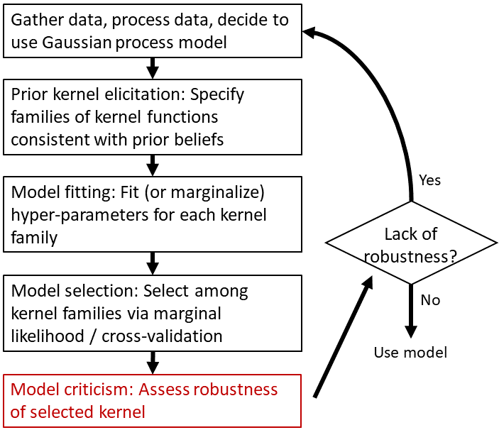
Gaussian processes (GPs) enable practitioners to estimate flexible functional relationships between predictors and outcomes. GPs have been used to monitor physiological vital signs in hospital patients (e.g. Cheng et al.,, 2020; Colopy et al.,, 2016; Futoma et al., 2017a, ; Futoma et al., 2017b, ), to estimate the health effects of exposure to airborne pollutants (e.g. Ferrari and Dunson,, 2020; Lee et al.,, 2017; Ren et al.,, 2021), and in many other medical and scientific settings. To use a GP for any application, a practitioner must choose a covariance kernel. The kernel determines the shape, smoothness, and other properties of the latent function of interest (Duvenaud,, 2014, Chap. 2). Ideally a user would specify a kernel that exactly encodes all of their prior beliefs about the latent function. In practice, a user often has only vague qualitative prior information and typically selects a kernel from a relatively small set of commonly used families. It seems plausible that other kernels could have been equally compatible with the user’s beliefs. When a user has no reason to prefer one kernel over another given their prior beliefs, we call the kernels qualitatively interchangeable. We would worry if substantive medical or scientific decisions changed when using a qualitatively interchangeable kernel: that is, if real-life decisions are non-robust to the choice of kernel. In this paper, we propose a workflow to assess the robustness of the GP posterior under qualitatively interchangeable choices of the kernel. Fig. 1 situates our work, an example of model criticism, in the modeling workflow.

Related work. Robustness and sensitivity of data analyses to data and model choice have been studied for decades (Andrews et al.,, 1972; Huber and Ronchetti,, 2009; Goodfellow et al.,, 2015). In the context of Bayesian methods, sensitivity to the choice of prior has been studied as well (Berger et al.,, 1994; Gustafson,, 1996; Berger,, 2000; Giordano et al.,, 2021). These works assess sensitivity by varying the prior within a small epsilon-ball around the user-specified prior with the intuition that a small ball will mostly contain priors that are acceptable alternatives to the user-specified prior. In contrast, we note that the class of qualitatively interchangeable kernels is actually the class of alternative priors of interest; we explicitly define and study sensitivity within this class.

Our focus on robustness to kernel choice stands in contrast to existing work on robustness in GPs, which focus on robustness to data perturbations (Kim and Ghahramani,, 2008; Hernández-Lobato et al.,, 2011; Jylänki et al.,, 2011; Ranjan et al.,, 2016; Bogunovic et al.,, 2018; Cardelli et al.,, 2019). Our focus is also distinct from that of works studying convergence rates (van der Vaart and van Zanten,, 2011; Teckentrup,, 2020; Wang and Jing,, 2021; Wynne et al.,, 2021) and asymptotic predictive equivalence (Stein,, 1993; Bevilacqua et al.,, 2019; Kirchner and Bolin,, 2021) for GP regression with misspecified kernels. These works do not examine how kernel choice affects non-linear functionals like posterior variances, do not study what happens in finite samples, and do not consider kernel choice as an issue of prior specification as we do. One might hope that automatic kernel discovery procedures (e.g. Benton et al.,, 2019; Duvenaud et al.,, 2013; Wilson and Adams,, 2013; Wilson et al.,, 2016) ostensibly obviate the need for careful kernel specification. However, choosing a particular kernel via model fitting does not preclude that many other kernels might satisfy a user’s prior beliefs. Indeed, we show that decisions made with kernels selected via modern model fitting can still exhibit non-robustness to kernel choice (Appendix E).

Model robustness versus model sensitivity. We emphasize that the goal of our work is to assess model robustness, which we now distinguish from model sensitivity. Model sensitivity measures how much our reported estimates change when we change our model. To assess model robustness, though, we also need to know how the model is being used. Often in applied analyses, many models reasonably reflect our prior beliefs and there is an application-specific threshold beyond which changes in reported estimates are deemed important; if our sensitivity is sufficiently high that we can observe an “important” change within the “reasonable” models, we say that our conclusion is (model) non-robust. While sensitivity is an objective and measurable quantity, model robustness is inherently qualitative and user-dependent. So the methods we present here are (and should be) qualitative and user-dependent. Although these general ideas are well-established (Berger et al.,, 1994; Insua and Ruggeri,, 2000), operationalizing them in the context of GPs is novel and challenging.

Our contributions. We propose and implement the first workflow to discover whether applied decisions based on a GP posterior are robust to the choice of the user-specified prior (i.e. the kernel). Our workflow proceeds as follows. (A) Keep expanding a class of appropriate kernels around the original kernel until some kernel in this class yields a substantively different decision. (B) Assess if this decision-changing kernel is qualitatively interchangeable with the original kernel. If the two kernels are interchangeable, we conclude the decision is not robust; a different decision could be reached with the same prior information. If the two kernels are not interchangeable, we cannot conclude non-robustness. We provide a practical implementation of steps (A) and (B). We demonstrate the practical utility of our workflow by discovering non-robustness in various applied uses of Gaussian processes: (1) predicting whether a hospital patient’s heart rate is alarmingly high, (2) predicting future carbon dioxide levels, and (3) classifying MNIST handwritten digits.

Figure 1: Where we sit in the modeling workflow.

2 OUR WORKFLOW

Setup and notation. Consider data $\mathcal{D}=\{(\bm{x}_{n},y_{n})\}_{n=1}^{N}$, with covariates $\bm{x}_{n}\in\mathbb{R}^{D}$ and outcomes $y_{n}\in\mathbb{R}.$ We model this data as $y_{n}\sim\mathcal{N}(f(x_{n}),\sigma^{2})$, where $f:\mathbb{R}^{D}\to\mathbb{R}$ is an unknown function, and $\sigma>0$ is a noise parameter. We place a zero-mean Gaussian process (GP) prior on $f$ with kernel $k$. Equivalently, we place a zero-mean GP prior on $\{y_{n}\}_{n=1}^{N}$ with kernel $k^{\prime}(x_{n},x_{m}):=k(x_{n},x_{m})+\sigma^{2}\delta_{nm}$. Going forward, we assume that kernels $k^{\prime}$ are comprised of a base kernel $k$ plus a noise term $\sigma^{2}\delta_{nm}$. Typical base kernels $k$ depend on a vector of hyperparameters $\theta_{k}$; for convenience, we define $\theta:=(\theta_{k},\sigma^{2})$. Unless stated otherwise, we assume that $\theta$ is estimated using maximum marginal likelihood estimation (MMLE). That is,

$$\hat{\theta}=(\hat{\theta}_{k},\hat{\sigma}^{2})=\operatorname*{arg\,max}_{\theta_{k},\sigma^{2}}p(y_{1:N},\mid\bm{x}_{1:N},\theta_{k},\sigma^{2}).$$ (1)

Let $k_{0}$ be the practitioner-chosen base kernel with MMLE hyperparameters $\hat{\theta}_{k}$. Let $F^{\star}(k)$ be any scalar functional of the posterior $f\mid\mathcal{D}$ that is a differentiable function of the base kernel $k$. Let the level $L\in\mathbb{R}$ represent a decision threshold in $F^{\star}(k)$. That is, we make one decision when $F^{\star}(k)\geq L$ and a different one when $F^{\star}(k)<L$. For example, let time be a single covariate, and let outcome be the resting heart rate of a hospital patient. $F^{\star}(k)$ could be the 95th percentile of the GP posterior at a given time; an alarm might trigger if $F^{\star}(k)$ is greater than $L=$130 bpm but not otherwise (Fidler et al.,, 2017). While many applied examples use $F^{\star}$ as a function of the posterior at a single test point $\bm{x}^{*}$, we stress that $F^{\star}$ can be any differentiable function of the posterior, e.g. the smooth maximum of means at a set of test points (Section 4).

We want to assess whether our decision would change if we used a different, but qualitatively interchangeable, kernel. Without loss of generality, we assume that $F^{\star}(k_{0})<L$. Then we can define non-robustness.

Definition 1.

For original kernel $k_{0}$, we say that our decision $F^{\star}(k_{0})<L$ is non-robust to the choice of kernel if there exists a kernel $k_{1}$ that is qualitatively interchangeable with $k_{0}$ and $F^{\star}(k_{1})\geq L$.

We emphasize that non-robustness as defined in Definition 1 is dependent on a number of user-dependent quantities – $k_{0}$, $F^{\star}$, $L$, and the user’s qualitative prior beliefs – as well as the particular observed data $\{(\bm{x}_{n},y_{n})\}_{n=1}^{N}$ and $\hat{\sigma}$. Also note that here we assess robustness to the specification of the GP governing the function $f$. In the present work, we do not assess sensitivity to the choice of i.i.d. normal noise around $f$ or the choice to use a GP prior at all. But allowing more components of the model to vary can only increase sensitivity. So if we find an analysis is non-robust using our current methods, the analysis would remain non-robust if we allowed more model variation.

Workflow overview. Our workflow is summarized in Algorithm 1. We start by defining a set $\mathcal{K}_{\varepsilon}$ of kernels that are “$\varepsilon$-near” $k_{0}$. We then optimize:

$$k_{1}(\varepsilon):=\operatorname*{arg\,max}_{k\in\mathcal{K}_{\varepsilon}}F^{\star}(k)$$

$$\varepsilon^{*}=\ \text{smallest}\ \varepsilon\ \text{s.t.}\ F^{\star}(k_{1}(\varepsilon))\geq L.$$ (2)

To find $\varepsilon^{*}$, we slowly increase $\varepsilon$ until $k_{1}(\varepsilon)$ changes our decision. We then check whether the decision-changing kernel, $k_{1}(\varepsilon^{*})$, is qualitatively interchangeable with $k_{0}$. It remains to precisely define a set of “$\varepsilon$-near” kernels and show that we can efficiently solve Eq. 2 (Section 2.1), and to provide ways to assess qualitative interchangeability (Section 2.2).

Note that although Algorithm 1 can detect non-robustness, it cannot certify robustness; it is possible, even though it may be unlikely, that there exists a qualitatively interchangeable kernel that the methodology has not detected but that still changes the decision. The inability to decisively declare an analysis robust is generally true of robustness analyses, and the present workflow is no exception. This observation is similar in spirit to classical hypothesis tests: a user can reject – but not accept – a null hypothesis.

Algorithm 1 Workflow for assessing robustness of GP inferences to kernel choice

1:Choose initial kernel $k_{0}$ using prior information.

2:Choose posterior quantity of interest $F^{\star}$. $\triangleright$ E.g. Posterior mean at test point $\bm{x}^{\star}$

3:Define decision threshold $L$ $\triangleright$ E.g. 130 bpm is an alarming resting heart rate

4:Define “$\varepsilon$-near” kernels $\mathcal{K}_{\varepsilon}$, for $\varepsilon>0$ $\triangleright$ Section 2.1

5:Solve Eq. 2 to get $k_{1}(\varepsilon^{*})$ $\triangleright$ Section 2.1

6:Assess if $k_{0}$ and $k_{1}(\varepsilon^{*})$ are qualitatively interchangeable. $\triangleright$ Section 2.2

7:if $k_{0}$ and $k_{1}(\varepsilon^{*})$ qualitatively interchangeable then return “$F^{\star}$ is non-robust to the choice of kernel.”

8:else  return “Did not find that $F^{\star}$ is non-robust to the choice of kernel.”

2.1 Nearby kernels and efficient optimization

We give two practical examples of how to choose $\mathcal{K}_{\varepsilon}$ in the present work and detail how to solve Eq. 2 in each case. First, we consider the case where we assume $k\in\mathcal{K}_{\varepsilon}$ should be stationary. Second, we allow non-stationary kernels $k\in\mathcal{K}_{\varepsilon}$.

Stationary kernels. Stationary kernels $k$ satisfy $k(\bm{x}_{n},\bm{x}_{m}):=k(\tau)$, where $\tau:=\bm{x}_{n}-\bm{x}_{m}$. By Bochner’s theorem, every stationary kernel can be represented by a positive measure (Rasmussen and Williams,, 2006, Thm. 4.1). In the kernel discovery literature, it is common to make the additional assumption that this measure has a density $S(\omega)=\int e^{-2\pi i\tau^{T}\omega}k(\tau)d\tau$ (Wilson and Adams,, 2013; Benton et al.,, 2019; Wilson et al.,, 2016). These authors show that the class of stationary kernels with a spectral density is a rich, flexible class of kernels. So, we optimize over spectral densities $S(\omega)$ – which are positive integrable functions on the reals – to recover stationary kernels. To make this optimization problem finite dimensional, we optimize the spectral density over a finite grid of frequencies $\omega$. All of our examples here use 1-dimensional covariates, so we use the trapezoidal rule to recover $k$. For our constraint set $\mathcal{K}_{\varepsilon}$, we use an $\varepsilon$ ball in the $\ell_{\infty}$ norm around the spectral density of $k_{0}$ for some $\varepsilon>0$. We find this simple constraint set to be sufficient for the examples in this paper; however, if users have specific prior beliefs about how the spectral density of $k_{1}$ should be constrained, this $\mathcal{K}_{\varepsilon}$ can be modified. We summarize this constraint set and the resulting optimization objective in Algorithm 2; see Appendix A for more details, including selection of $\omega_{1},\dots,\omega_{G}$.

Algorithm 2 Objective and $\mathcal{K}_{\varepsilon}$ for stationary kernels

1:Objective

2:Input: Frequencies $\omega_{1},\dots,\omega_{G}$, and density values $S(\omega_{1}),\dots,S(\omega_{G})$.

3:Approximate the integral $k(\tau)=\int e^{2\pi i\tau^{T}\omega}S(\omega)d\omega$ at $\tau$ needed to evaluate $F^{\star}$ (e.g. trapezoidal rule).

4:return $F^{\star}(k)$.

1:

2:Constraint on $S(\omega_{1}),\dots,S(\omega_{G})$ defining $\mathcal{K}_{\varepsilon}$

3:Input: Frequencies $\omega_{1},\dots,\omega_{G}$, density values $S(\omega_{1}),\dots,S(\omega_{G})$, constraint set size $\varepsilon>0$.

4:Compute $S_{0}(\omega_{1}),\dots,S_{0}(\omega_{G})$ (spectral density of $k_{0}$) via trapezoidal rule or exact formula.

5:if Spectral density $S$ of $k$ satisfies:

$$\max\big{(}0,(1-\varepsilon)S_{0}(\omega_{g})\big{)} \leq S(\omega_{g})\leq(1+\varepsilon)S_{0}(\omega_{g}),$$

$$\quad g=1,\dots,G.$$

 then return “In constraint set”

6:Else return “Not in constraint set”

Non-stationary kernels. In many modeling problems, stationarity may be a choice of convenience rather than prior conviction, or one may believe non-stationarity is probable. In either case, we wish to allow non-stationary kernels in the neighborhood $\mathcal{K}_{\varepsilon}$. A convenient technique for constructing non-stationary kernels relies on input warping (Rasmussen and Williams,, 2006, Sec 4.2.3). Given a kernel $k_{0}$ and a non-linear mapping $g$, we define a perturbed kernel $k(\bm{x},\bm{x}^{\prime})=k_{0}(g(\bm{x}),g(\bm{x}^{\prime}))$. This construction guarantees that the perturbed kernel $k$ is a kernel function as long as $k_{0}$ is a valid kernel. We let the function $g$ have parameters $w$ and set $g(\bm{x};w):=\bm{x}+h(\bm{x};w),$ where $h:\mathbb{R}^{D}\rightarrow\mathbb{R}^{D}$ is a small neural network with weights $w$. By controlling the magnitude of $h$, we can control the deviations from $k_{0}$.

We could optimize the weights $w$ under the constraint $\|h(\bm{x};w)\|_{2}^{2}\leq\varepsilon$. However, it is unclear how to enforce this constraint. Instead, we select a grid of $M$ points $\tilde{\bm{x}}_{1},\ldots,\tilde{\bm{x}}_{M}\in\mathbb{R}^{D}$ and add a regularizer to our objective, $\frac{1}{\varepsilon}\frac{1}{M}\sum_{m=1}^{M}||h(\tilde{\bm{x}}_{m},w)||_{2}^{2},$ where $\varepsilon$ controls the regularization strength. We find using a grid of points to be a computationally cheap, mathematically simple, and empirically successful approximation to regularizing the entire function. We summarize our objective as a function of the network weights $w$ in Algorithm 3. Note that we have also changed our objective to include a generic loss $\ell$; some care needs to be taken to ensure that the optimal $k_{1}(\varepsilon)$ is finite. See Sections 4 and 5 for specific implementations of $\ell$. Given the $\hat{w}$ minimizing the objective in Algorithm 3, we set $k_{1}(\varepsilon)(\bm{x},\bm{x}^{\prime})=k_{0}(g(\bm{x};\hat{w}),g(\bm{x}^{\prime};\hat{w}))$.

Algorithm 3 Objective for non-stationary kernels

1:Input: Grid points $\tilde{\bm{x}}_{1},\dots,\tilde{\bm{x}}_{M}$, regularizer strength $\varepsilon>0$, neural network weights $w\in\mathbb{R}^{D}$.

2:Define neural network $h(x;w)$ with weights $w$.

3:Define $k(\bm{x},\bm{x}^{\prime}):=k_{0}(\bm{x}+h(\bm{x};w),\bm{x}^{\prime}+h(\bm{x}^{\prime};w))$.

4:return $\ell(k;F^{\star},L)+\frac{1}{\varepsilon}\frac{1}{M}\sum_{m=1}^{M}||h(\tilde{\bm{x}}_{m};w)||_{2}^{2}$

2.2 Assessing qualitative interchangeability

We introduce two assessments, similar to prior predictive checks (Gabry et al.,, 2019), to assess qualitative interchangeability between two kernels $k_{0}$ and $k_{1}$.

Visual comparison of prior draws. When the covariates $\bm{x}$ are low-dimensional, we can plot a small collection of functions drawn from each of the two distributions $\mathcal{GP}(0,k_{0})$ and $\mathcal{GP}(0,k_{1}).$ To ensure that visual differences between the priors are due to actual differences in the kernels and not randomness in the draws, we use noise-matched prior draws. To define noise-matched draws, recall that one can draw from an $N$-dimensional Gaussian distribution $\mathcal{N}(0,\Sigma)$ by computing the Cholesky decomposition $LL^{\top}=\Sigma$; if we draw $z\sim\mathcal{N}(0,I_{N})$, we then have $Lz\sim\mathcal{N}(0,\Sigma)$. We say that draws from two multivariate Gaussians are noise-matched if they use the same $z$.

If the user believes the two plots express the same qualitative information, the kernels are qualitatively interchangeable under this test. A potential drawback to this method is that when covariates are high-dimensional, it may be difficult to effectively visualize prior draws. We address this concern next.

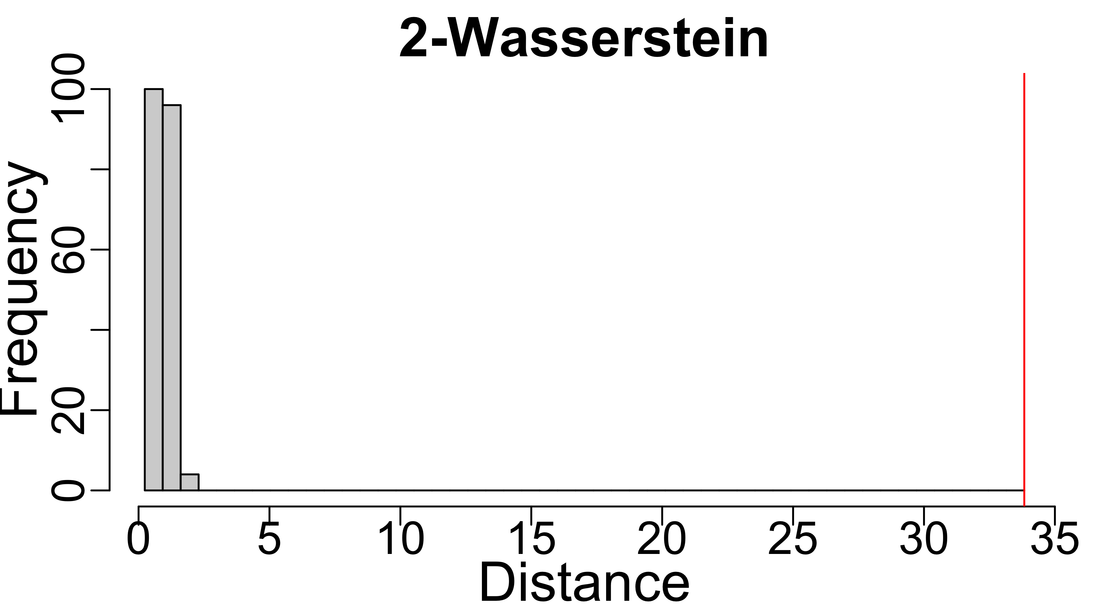
Comparison through Wasserstein distances. Our second test for qualitative interchangeability computes a distance between the priors $\mathcal{GP}(0,k_{0})$ and $\mathcal{GP}(0,k_{1})$ and uses hyperparameter uncertainty in $k_{0}^{\prime}$ to help users understand whether this distance is large. Although directly computing distances between Gaussian processes is difficult, we can compare the $\mathcal{GP}(0,k_{0}^{\prime})$ and $\mathcal{GP}(0,k_{1}^{\prime})$ priors on the set $\{\bm{x}_{1},\dots,\bm{x}_{N}\}$. On this set, these priors are just multivariate normal distributions with covariance matrices equal to the Gram matrices $k_{0}(X,X)+\hat{\sigma}^{2}I_{N}$ and $k_{1}(X,X)+\hat{\sigma}^{2}I_{N}$, where $X\in\mathbb{R}^{N\times D}$ is the matrix of covariates. Going forward, we denote by $d(k_{0}^{\prime},k_{1}^{\prime})$ the 2-Wasserstein distance between these multivariate normals. We use the 2-Wasserstein as a default choice because it directly corresponds to quantities easily interpretable by users: a 2-Wasserstein distance of $\alpha$ means that coordinate-wise standard deviations differ by at most $\alpha$ (Thm. 3.4 Huggins et al.,, 2020). While we feel the 2-Wasserstein distance provides a good default choice of $d$, users can substitute other choices if there are application-specific reasons why another distance is more meaningful. In Appendix G, we discuss this possibility and also show that our results are typically not sensitive to the choice of $d$ throughout our experiments.

Even though users may be able to understand the meaning of $d(k_{0}^{\prime},k_{1}^{\prime})$, users may still have difficulty understanding whether $d(k_{0}^{\prime},k_{1}^{\prime})$ is large or not. In particular, users may not have an understanding of the scale of $d$. To help users understand the scale of $d$, we use a particular form of uncertainty about $k_{0}^{\prime}.$ Since we learn the hyperparameters $\hat{\theta}$ of $k_{0}^{\prime}$ from finite data, there remains frequentist sampling uncertainty about $\hat{\theta}$, which we denote by the distribution $q(\hat{\theta}).$ We make $R$ i.i.d. draws $\{\theta^{(r)}\}_{r=1}^{R}$ from $q(\hat{\theta})$ (or an approximation of $q$). For each $r$, we compute $d(k_{0}^{\prime},k^{{}^{\prime}(r)})$, where $k^{{}^{\prime}(r)}$ has the same functional form as $k_{0}^{\prime}$ but with hyperparameters $\theta^{(r)}$ instead of $\hat{\theta}$. To the extent that bootstrap resamples capture frequentist sampling variability, users should be as open to using most $k^{{}^{\prime}(r)}$ as they are to using $k_{0}’$. Thus if $d(k_{0}^{\prime},k_{1}^{\prime})$ is small relative to the $d(k_{0}^{\prime},k^{{}^{\prime}(r)})$’s, we say that $k_{0}$ and $k_{1}$ are qualitatively interchangeable. Note that we cannot necessarily reject qualitative interchangeability if $d(k_{0}^{\prime},k_{1}^{\prime})$ is large relative to the $d(k_{0}^{\prime},k^{{}^{\prime}(r)})$. For example, if we observe more and more data $(\bm{x},y)$ with the $\bm{x}$’s contained in a compact region of $\mathbb{R}^{D}$, then we expect our uncertainty about the hyperparameters to go to zero. Thus, for fixed $k_{1}^{\prime}$, $d(k_{0}^{\prime},k_{1}^{\prime})$ will eventually always be large relative to the $d(k_{0}^{\prime},k^{{}^{\prime}(r)})$.

In our experiments, we make the following choices. Unless otherwise stated, we approximately sample from $q(\hat{\theta})$ by drawing bootstrap samples from $\{(\bm{x}_{n},y_{n})\}_{n=1}^{N}$ and re-solving Eq. 1 with the bootstrapped data. We construct a histogram of the 2-Wasserstein distance between $k^{{}^{\prime}(r)}$ and $k_{0}^{\prime}$ across $r$, with a marker indicating the position of the 2-Wasserstein between $k_{1}^{\prime}$ and $k_{0}^{\prime}$. If the marker lies to the left of or within the histogram, we conclude that $k_{1}$ and $k_{0}$ are qualitatively interchangeable.

2.3 Workflow illustration on synthetic data

Figure 2: (Far left): Synthetic data. Vertical lines denote our interpolation point ($\bm{x}^{\star}=2.0$) and extrapolation point ($\bm{x}^{\star}=6.25$). (Center left:) Draws from the original prior $\mathcal{GP}(0,k_{0})$. (Center right): Draws from $\mathcal{GP}(0,k^{(ex)})$. (Far right): Draws from $\mathcal{GP}(0,k^{(in)})$. The prior draws are noise-matched to the draws from $k_{0}$ (Section 2.2).

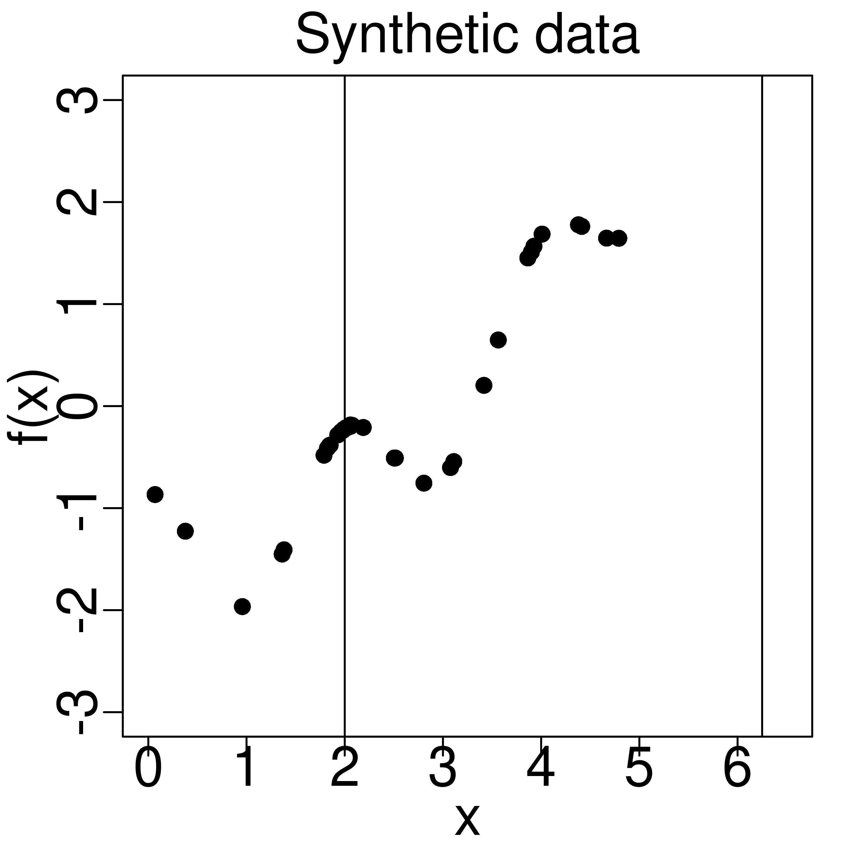
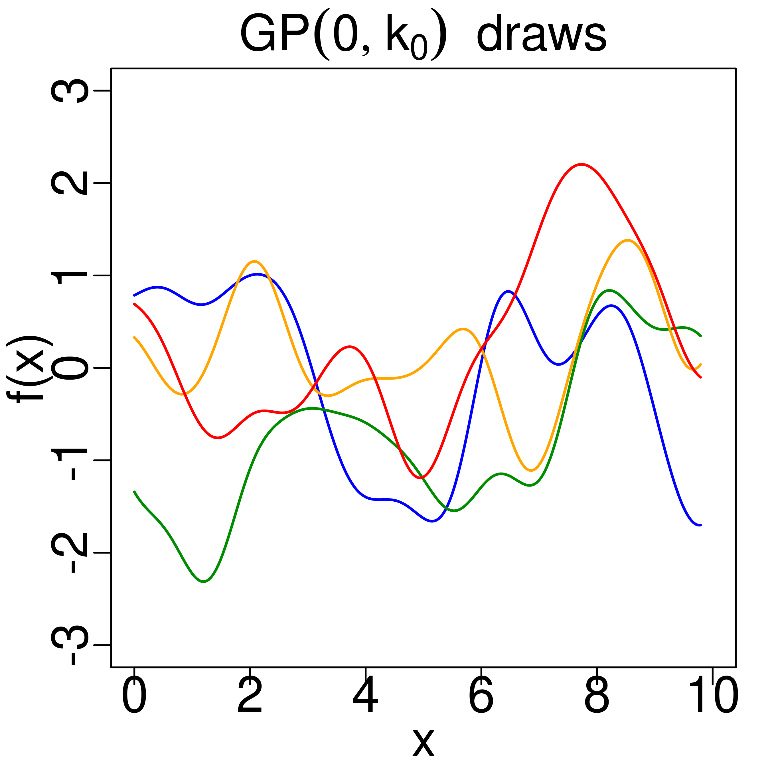
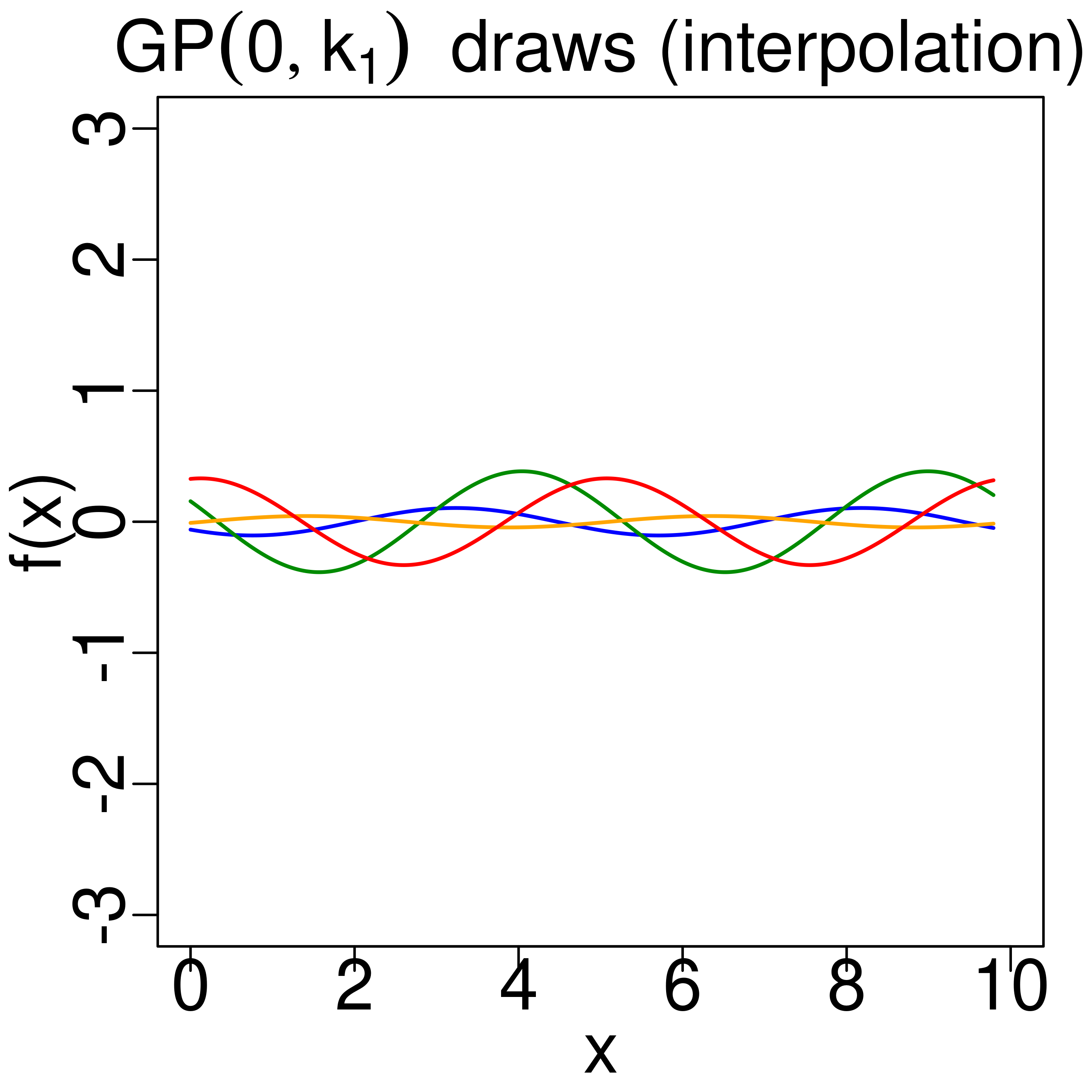
Data and decision. Before turning to real data, we illustrate our workflow with a synthetic-data example. We consider $N=24$ data points with a single covariate; see the leftmost panel of Fig. 2. We assume we have qualitative prior beliefs that (i) $f$ is smooth and (ii) our beliefs about $f$ are invariant to translation along the single covariate (stationarity). In this case a plausible kernel choice is a squared exponential kernel: $k_{0}(x_{1},x_{2})=\exp\big{(}-0.5(x_{1}-x_{2})^{2}/\ell\big{)}$. We estimate $k_{0}$’s hyperparameter $\ell$ and the noise parameter $\sigma$ via maximum marginal likelihood estimation (MMLE). Four draws from the resulting prior are shown in the second panel of Fig. 2.

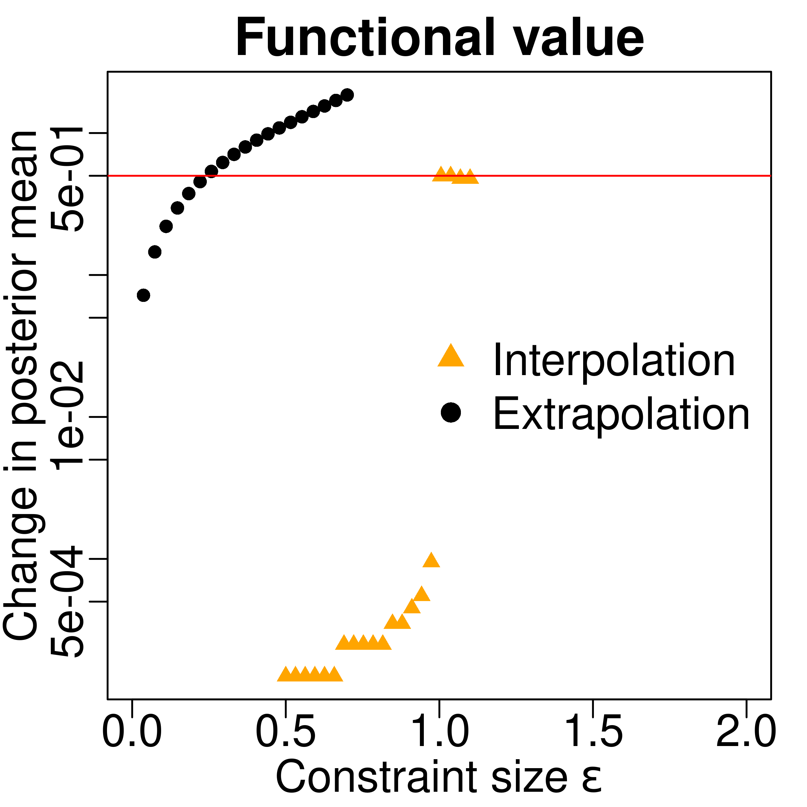
For the purposes of this illustration, we will look at two separate decisions. One is at $\bm{x}^{\star}=2.0,$ which is within a dense region of training data (interpolation). And one is at $\bm{x}^{\star}=6.25,$ which is outside the range of the training data (extrapolation). Our functional of interest at either point will be the change in posterior mean, $F^{\star}(k):=\mu(\bm{x}^{\star},k)-\mu(\bm{x}^{\star},k_{0})$, where $\mu(\bm{x}^{\star},k)$ is the posterior mean at test point $x$ under kernel $k$. We suppose that we would make a different decision if the posterior mean changed by a small amount: $F^{\star}\geq L=0.01$. Intuitively, we expect only minor changes to the prior to be needed to bring about such a posterior change in our extrapolation example. In our interpolation example, we expect a substantial change to the prior to be needed to change the posterior even a small amount, as we have intentionally chosen our interpolation point to sit in a region of dense training data. We now show that the output of our method matches this intuition in both cases.

Nearby kernels. Since we assume stationarity, we choose Algorithm 2 at line 4 of Algorithm 1. Fig. 3 (first panel) shows what happens as we increase $\varepsilon$ to solve Eq. 2. The black dots (extrapolation) quickly cross the decision threshold line, so we have solved Eq. 2. The orange triangles (interpolation) show that a larger $\varepsilon$ is required to breach our decision threshold.

Figure 3: (Left): Maximal value of the function $F^{\star}$ as a function of constraint set $\varepsilon.$ Comparison of the 2-Wasserstein distance between $k_{0}(X,X)$ and $k_{1}(X,X)$ to the posterior variation due to hyperparameter uncertainty for extrapolation (middle) and interpolation (right). The red line corresponds to our decision-changing kernel $k_{1}$.

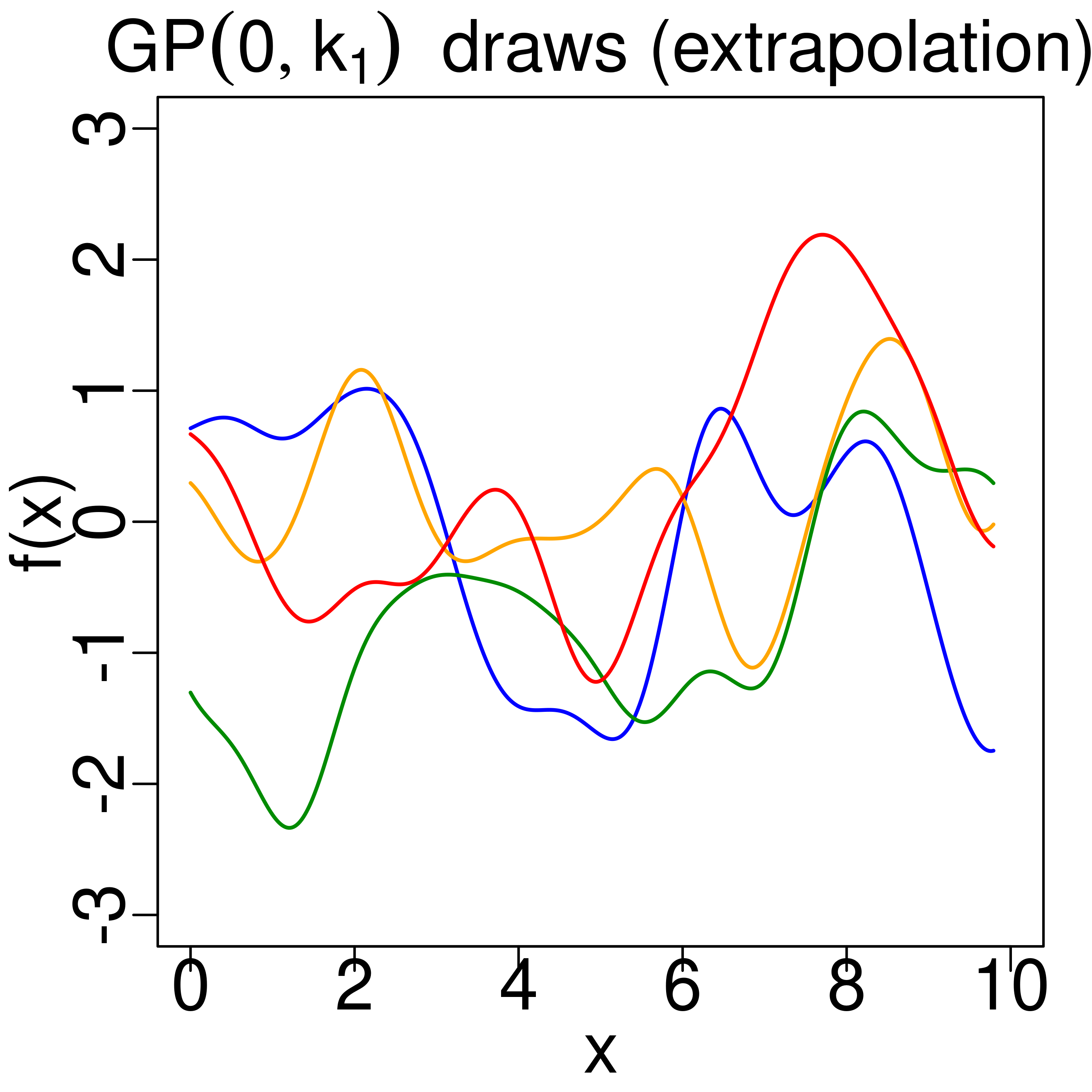
Qualitative interchangeability: Visual comparison of prior draws. We now demonstrate our first test for qualitative interchangeability. For our extrapolation example ($\bm{x}^{\star}=6.25$), let $k^{(ex)}$ be the solution to Eq. 2. The third panel of Fig. 2 shows prior draws with $k^{(ex)}$; the draws are noise-matched with the second panel. $k^{(ex)}$ is so similar to $k_{0}$ that the two sets of prior draws (second and third panels) are visually indistinguishable. We say that $k^{(ex)}$ is qualitatively interchangeable with $k_{0}$.

Let $k^{(in)}$ be the solution to Eq. 2 for our interpolation example ($\bm{x}^{\star}=2.0$). The fourth panel of Fig. 2 shows prior draws with $k^{(in)}$; the draws are noise-matched with the second panel. Again, by design, both sets of draws (second and fourth panels) are stationary and smooth. However, the magnitudes of peaks and troughs with $k^{(in)}$ are much smaller than those with $k_{0}$. Thus, we say that $k^{(in)}$ is not qualitatively interchangeable with $k_{0}$ under this test.

Qualitative interchangeability: 2-Wasserstein comparison. Histograms of the 2-Wasserstein distance between $k_{0}$ and $k^{(r)}$ appear in Fig. 3. $k^{(ex)}$ sits within the histogram of alternative kernels generated via hyperparameter uncertainty (center), whereas $k^{(in)}$ sits outside this uncertainty region (right). As in our prior visualization comparison, we say that $k^{(in)}$ is not qualitatively interchangeable with $k_{0}$ under our 2-Wasserstein comparison, whereas $k^{(ex)}$ is.

Finally, following our workflow, we conclude that our extrapolation example is non-robust to the choice of kernel in the sense of Definition 1. On the other hand, in our interpolation example, we do not find non-robustness.

3 STATIONARY PERTURBATIONS TO A MODEL OF HEART RATES

We now provide an example of using our workflow to assess the sensitivity of GP predictions of hospital patient deterioration. Colopy et al., (2016) use a GP to model individual patients’ heart rates and predict potentially troubling behavior at a future time $\bm{x}^{\star}$. We check whether this prediction is robust to kernel choice.

Figure 4: Sensitivity of heart rate analysis in Section 3. (Top row): (left) Observed data. (middle and right) Noise-matched draws from original prior $\mathcal{GP}(0,k_{0})$ (middle) and alternative prior $\mathcal{GP}(0,k_{1})$ (right). (Bottom row): (left) Comparison of the difference between $k_{0}$ and $k_{1}$ (red line) to bootstrapped hyperparameter uncertainty (histogram). (middle) Once we expand the constraint set to $\varepsilon=0.24$ the predicted 95% quantile of heart rate at $\bm{x}^{\star}$ exceeds 130 bpm (red line). (right) Comparison of posterior distributions $f(\bm{x}^{\star})\mid\mathcal{D}$ computed using $k_{0}$ (blue) and $k_{1}(\varepsilon^{*})$ (red).

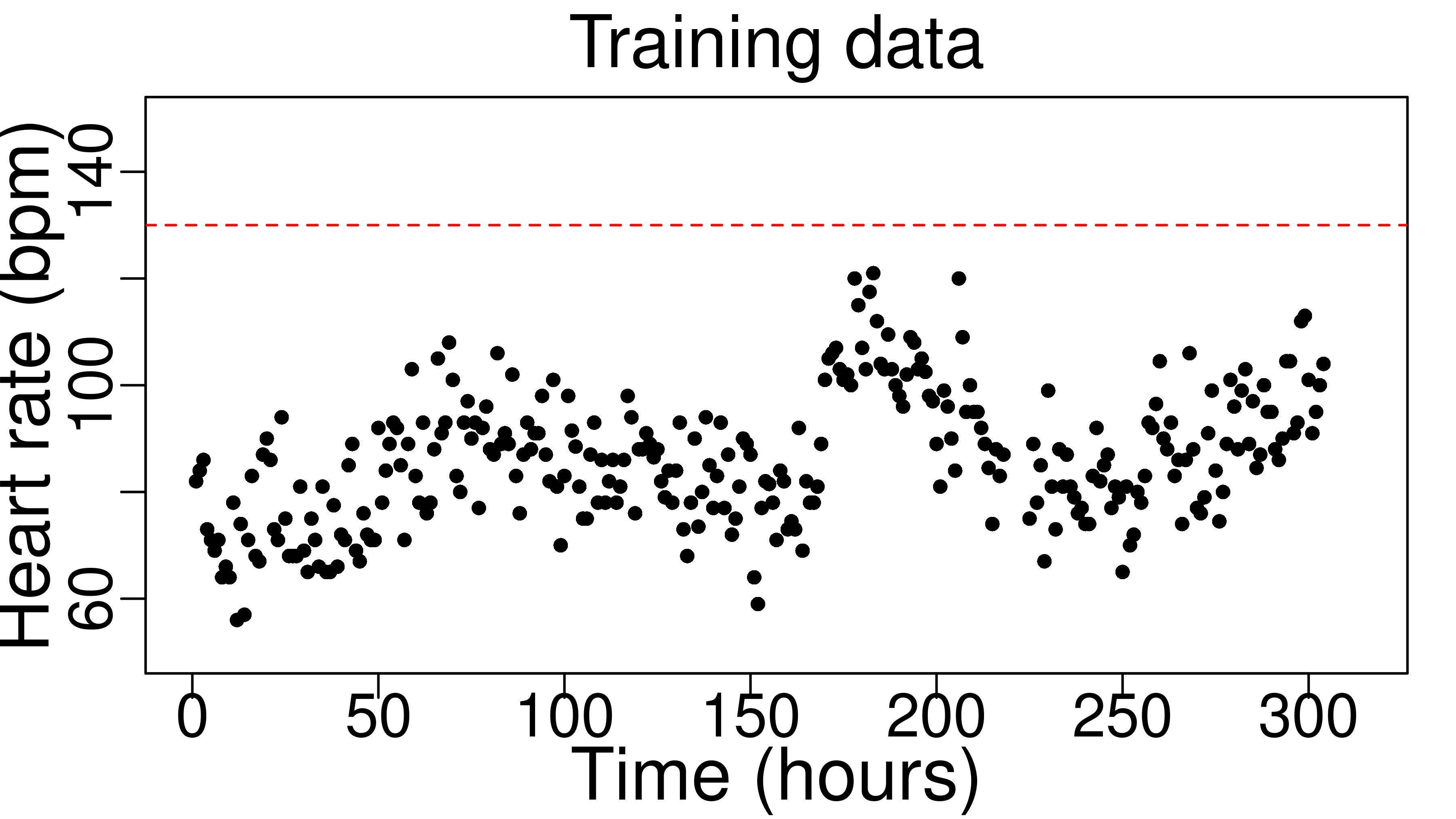
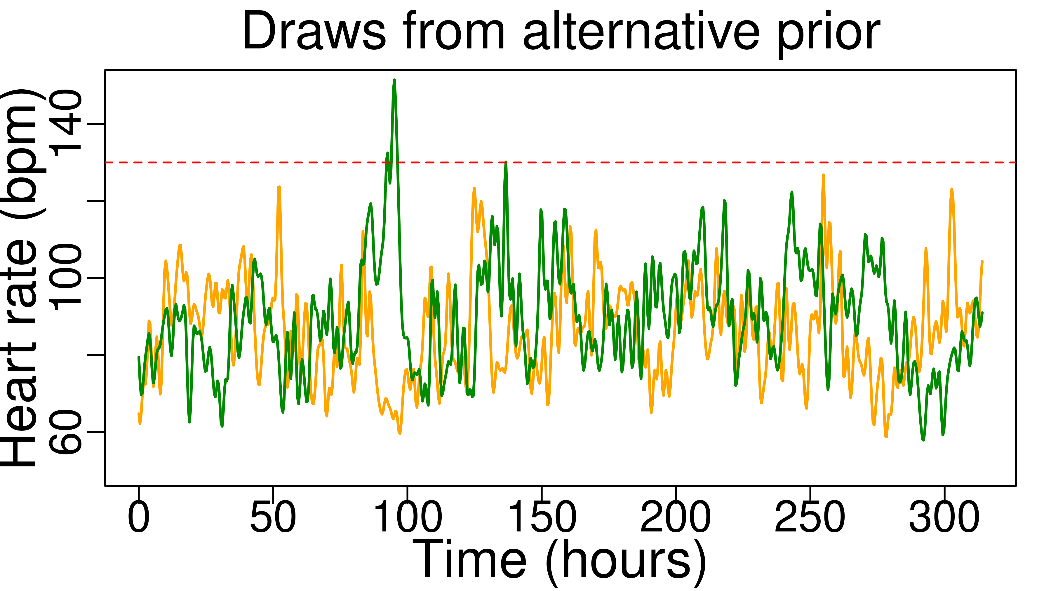
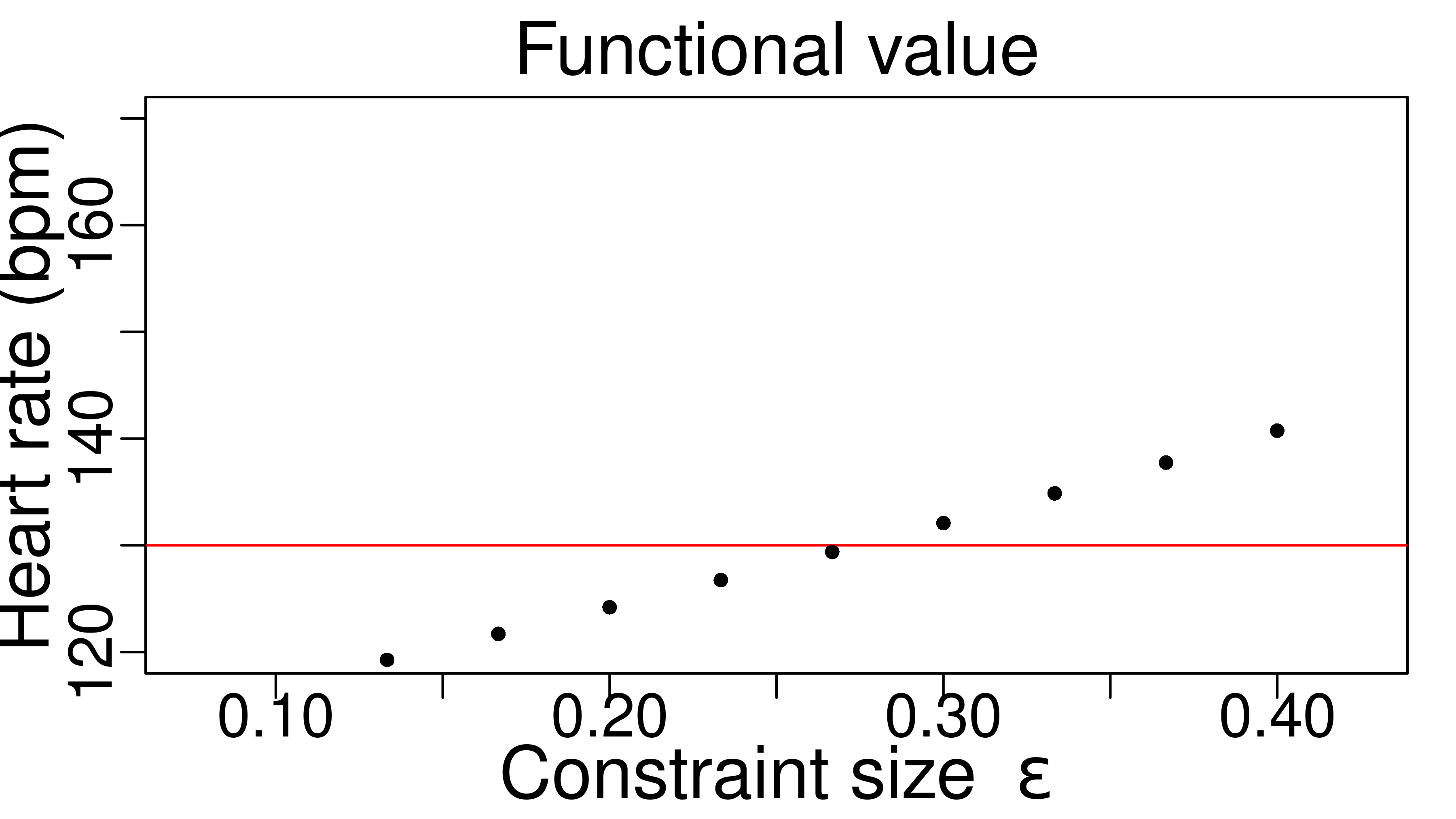
Data, model, and decision. Colopy et al., (2016) observe an outcome, heart-rate data measured in beats per minute (bpm), as a function of one covariate, time. The authors choose their GP model to have mean equal to zero and a kernel equal to the sum of a squared exponential and Matérn(5/2) kernel; see Appendix C. We fit the overall kernel’s hyperparameters via MMLE and refer to the resulting kernel as $k_{0}$. Some standard hospital alarm systems activate at 130 bpm (Fidler et al.,, 2017), a threshold describing a worryingly-high resting heart rate. So we consider the task of predicting whether the 95th percentile of the GP posterior is above $L=130$ bpm. Most predictions in Colopy et al., (2016) take place 1.5 hours in the future, so we set $F^{\star}$ to be the 95th quantile at 1.5 hours hours after the last observed data point. The data from Colopy et al., (2016) is confidential, so we use heart-rate data from the 2019 Computing in Cardiology Challenge (Reyna et al.,, 2019; Goldberger et al.,, 2000).

Prior beliefs. Colopy et al., (2016) note that $k_{0}$ encodes the belief that “longer trends (on the order of hours) are governed by the smooth RBF kernel, while minutely variations in [heart-rate] are governed by a twice-differentiable Matérn(5/2) kernel.” Although Colopy et al., (2016) are not explicit about assuming stationarity, we presume it is a reasonable prior belief here; while we expect that a patient’s heart rate may change while in the hospital, our prior beliefs about the timing of any changes may be roughly uniform. We thus choose $\mathcal{K}_{\varepsilon}$ according to the stationary specification in Section 2.1.

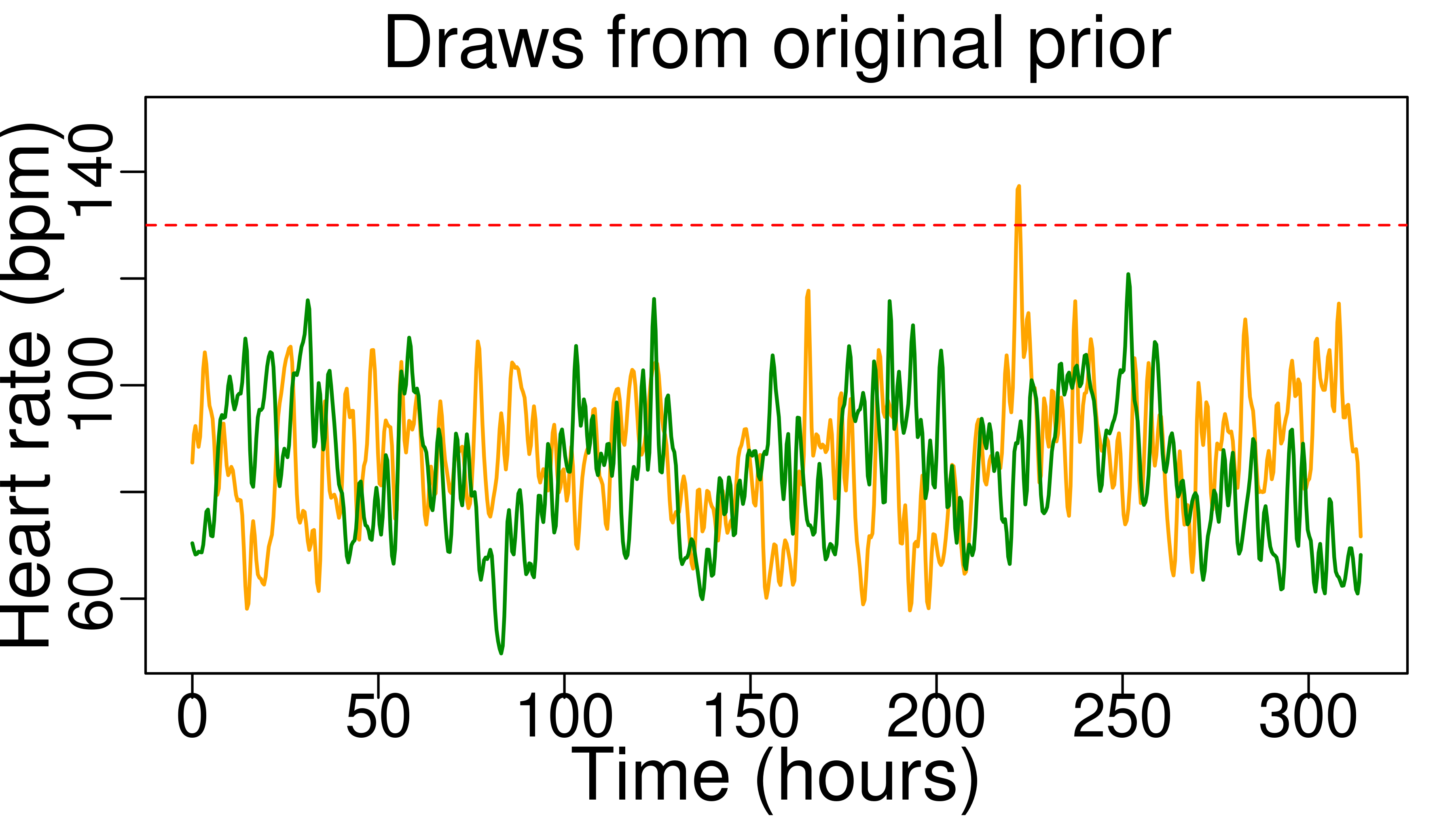
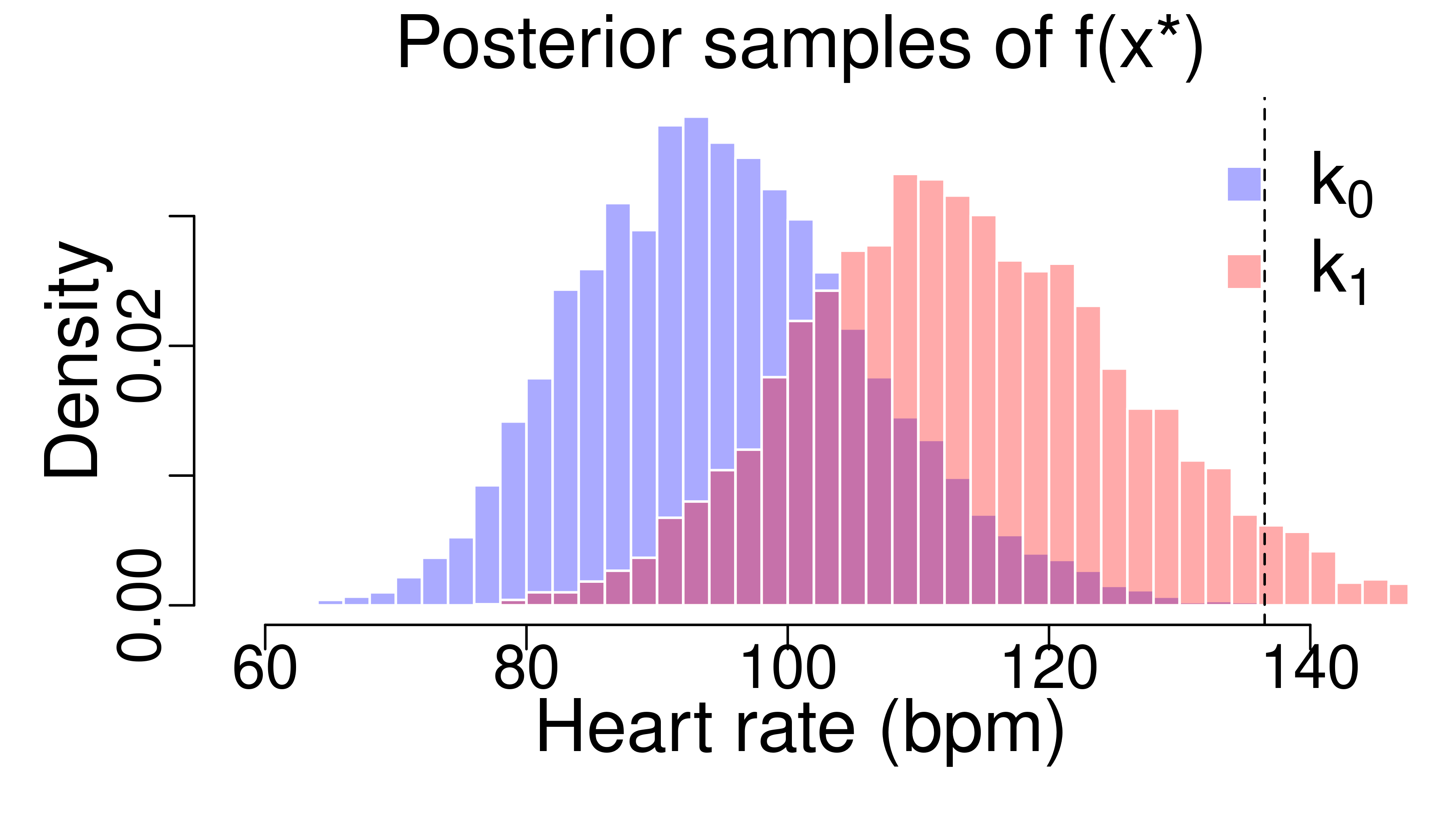
Robustness. Fig. 4 depicts our workflow (Algorithm 1) in action. We solve Eq. 2 to obtain $k_{1}(\varepsilon^{*})$ such that $F^{\star}(k_{1}(\varepsilon^{*}))\geq L$. We then compare noise-matched samples from the priors using $k_{0}$ and $k_{1}(\varepsilon^{*})$. The noise-matched samples do not clearly represent different pieces of prior information; both prior plots display functions that are fairly rough with similar length scales. Finally, we see that the 2-Wasserstein distance between $k_{0}$ and $k_{1}(\varepsilon^{*})$ is substantially smaller than the 2-Wasserstein distance between $k_{0}$ and kernels from the sampling uncertainty in the MMLE hyperparameters. Our tests suggest $k_{0}$ and $k_{1}(\varepsilon^{*})$ are qualitatively interchangeable; we conclude that the prediction that $F^{\star}$ will breach the alarm threshold is non-robust in the sense of Definition 1. While this outcome may be surprising, it is not entirely unintuitive. The patient’s heart rate is trending up toward the end of the observed data. In Appendix C, we show an example where the observed data is trending downward at the end of the observed data. In the latter case, the resulting kernel $k_{1}(\varepsilon^{*})$ fails both of our tests of qualitative interchangeability and so we cannot conclude non-robustness.

4 NON-STATIONARY PERTURBATIONS TO A MODEL OF CO₂ LEVELS

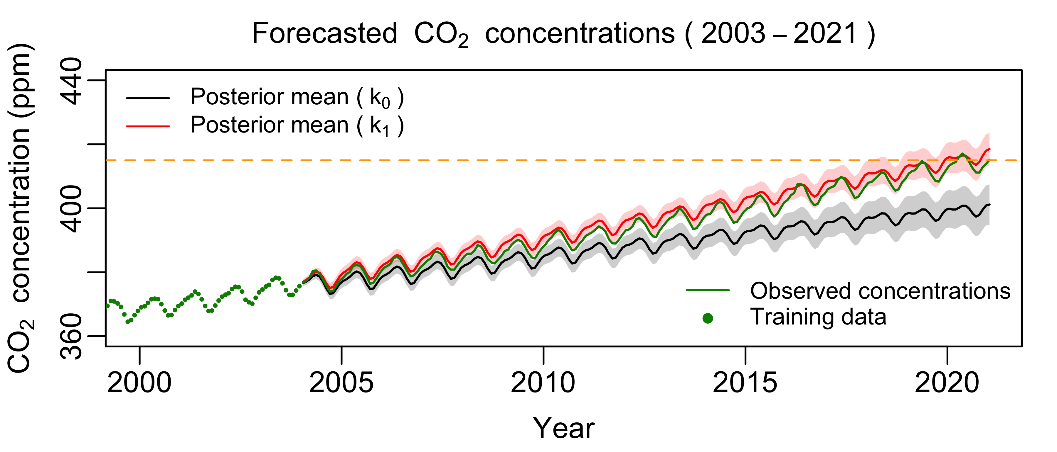
In a now-classic analysis of carbon dioxide (CO₂) levels at Mauna Loa, Rasmussen and Williams, (2006) predicted future CO₂ levels based on data up to 2003. With data up to 2021, we can now see that the Rasmussen and Williams, (2006) analysis substantially underestimates present-day CO₂ levels; compare the gray region (99.7% quantile of the original predictions) to the green (true levels) in Fig. 5. In this section, we show that this prediction of modern CO₂ levels is non-robust to kernel choice. In Appendix E, we repeat the analysis with a kernel whose structure is learned using the automatic statistician (Duvenaud et al.,, 2013) and discover similar lack of robustness.

Data, model, and decision. At the present day, monthly data for CO₂ emissions is available from the year 1958 through 2021. But Rasmussen and Williams, (2006) use training data up to 2003. Rasmussen and Williams, (2006) use a kernel that is a sum of four basic kernels, where each term plays a specific role; e.g. a periodic term models the periodic seasonal trend in CO₂ levels. See Appendix D for a full description of the kernel. We take this kernel with hyperparameters fit via MMLE as our $k_{0}$. Actual CO₂ levels breached 415 ppm for the first time in human history (Solly,, 2019) in 2019. Under $k_{0}$, this level lies more than three standard deviations away from the predicted means in all of 2019. To see whether a qualitatively interchangeable $k_{1}$ would better predict modern CO₂ levels, we let $F^{\star}$ be the smooth-max of all posterior means in 2019. We will say the posterior has substantively changed if $F^{\star}\geq L=415$ ppm.

Prior beliefs. While $k_{0}$ is a stationary kernel we might also have non-stationary prior information such as known historical or expected future developments in climate policy or technology. So we choose $\mathcal{K}_{\varepsilon}$ according to the non-stationary input-warping specification in Section 2.1. For our regularizer grid, we use 600 evenly spaced points $\tilde{\bm{x}}_{1},\dots,\tilde{\bm{x}}_{600}$ between 1958 and 2021 to control $h$ throughout our time period of interest. Input warping the entire kernel as $k=k_{0}(g(\bm{x}),g(\bm{x}^{\prime}))$ would violate an important piece of prior information that we have about CO₂ levels: CO₂ has a regular seasonality, with minimal levels in the winter and maximal levels in the summer. The original $k_{0}$ accounts for this feature of the data with a periodic term; Fig. 5 (top) shows that this periodicity lines up very well with the training data. To produce an alternative kernel that accounts for this piece of prior knowledge, we leave the periodic portion of the kernel unwarped. To parameterize $g$, we use a fully connected network with two hidden layers, $50$ units, and ReLU nonlinearities. To ensure the optimal $k_{1}$ is finite, we take the loss in Algorithm 3 to be $\ell(k;F^{\star},L)=(F^{\star}(k)-L)^{2}$ to guarantee our objective is bounded below.

Figure 5: Sensitivity of the Mauna Loa analysis in Section 4. (Top-left): Predictions made with the original kernel $k_{0}$ (black) and a qualitatively interchangeable kernel $k_{1}$ (red). (Top-right): $F^{\star}$, the mean CO₂ level in June 2020, as a function of $\varepsilon$. (Bottom): Noise-matched draws from a $\mathcal{GP}(0,k_{0})$ (left) and $\mathcal{GP}(0,k_{1}(\varepsilon^{*}))$ (right) prior. See Appendix D for a closer inspection of each prior draw.

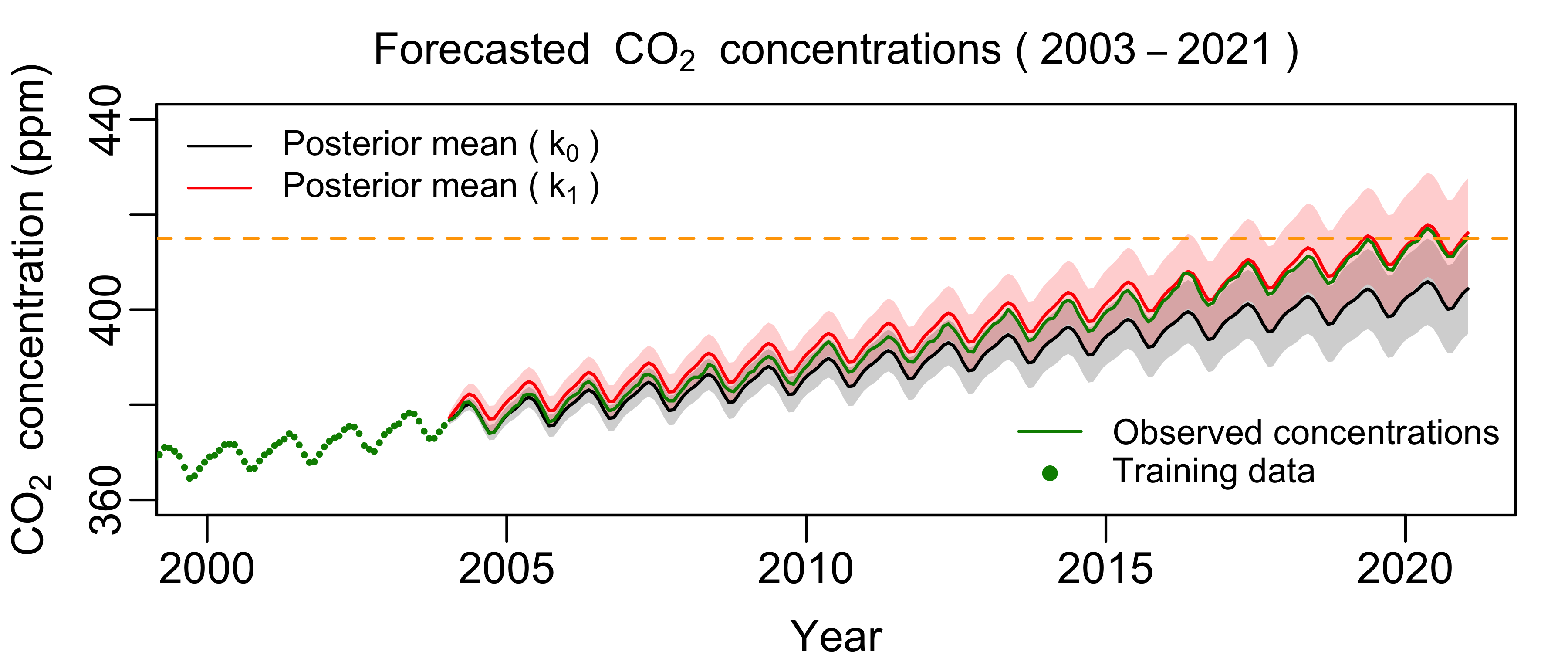
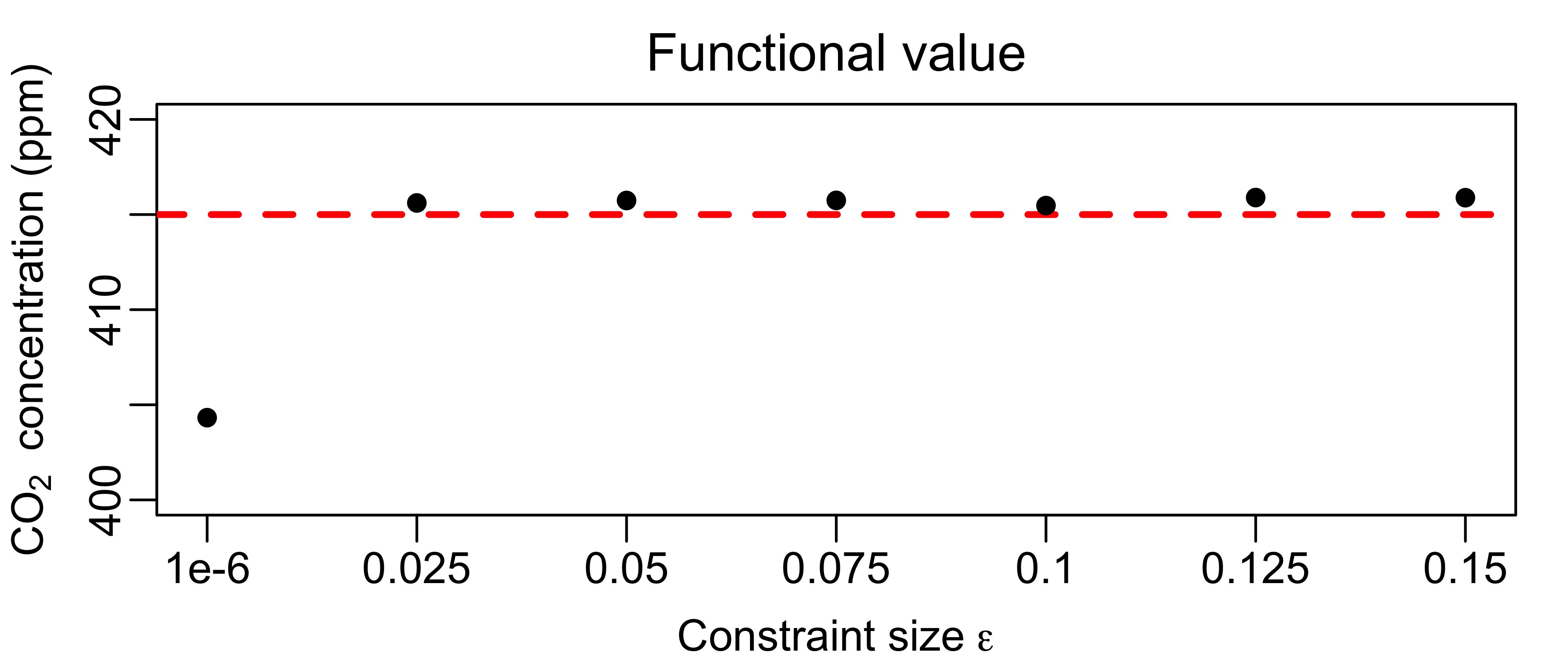
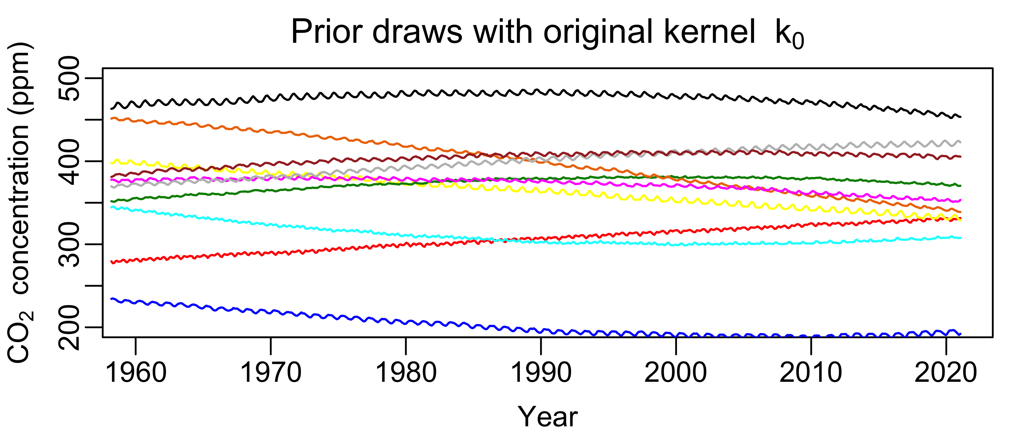
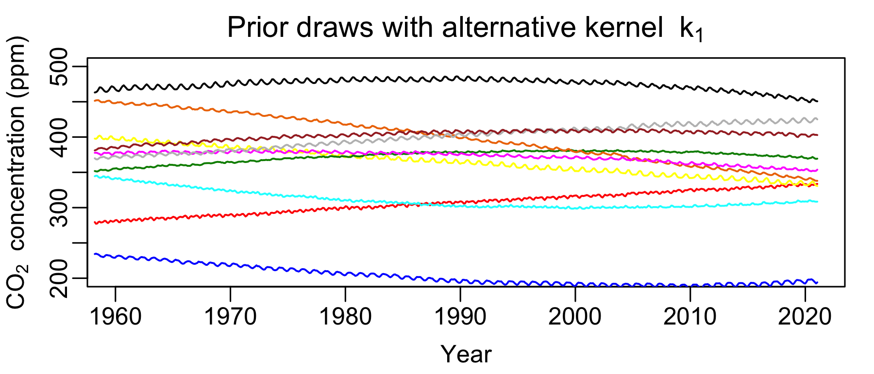
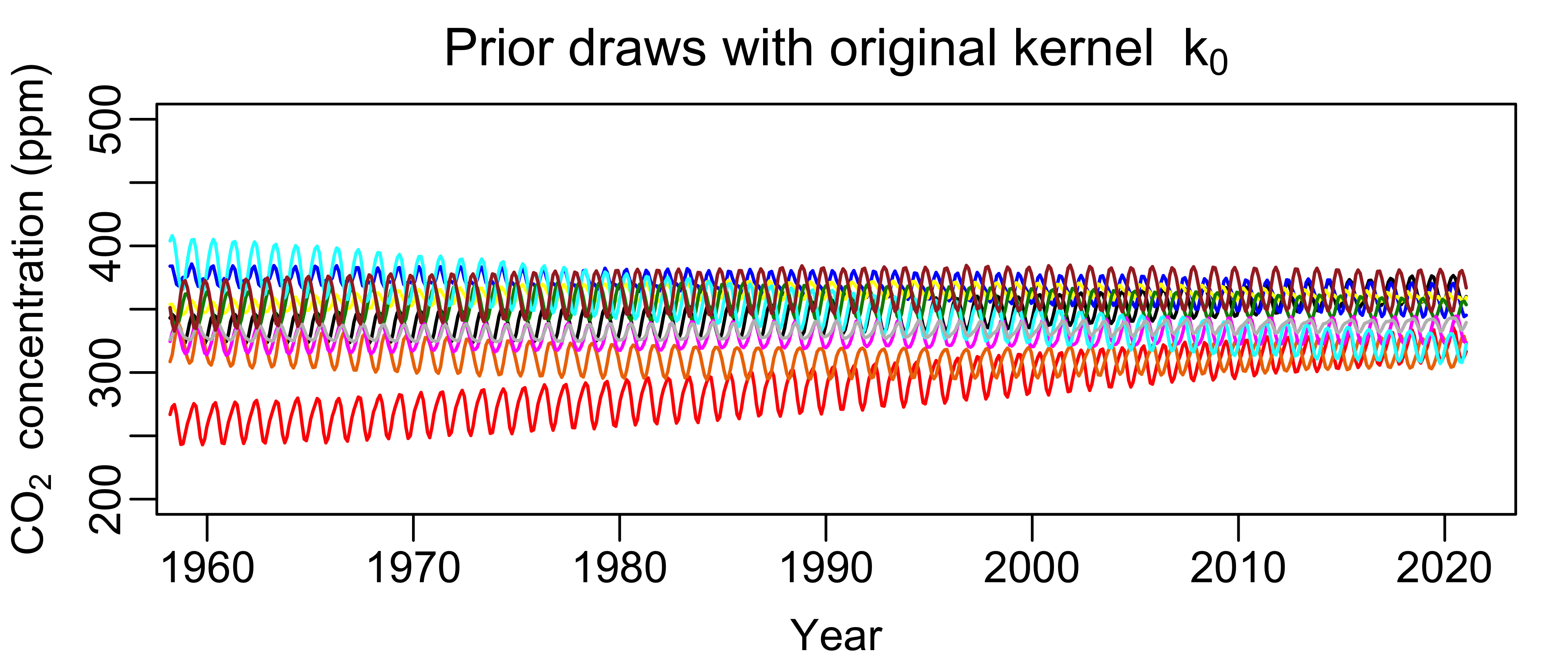
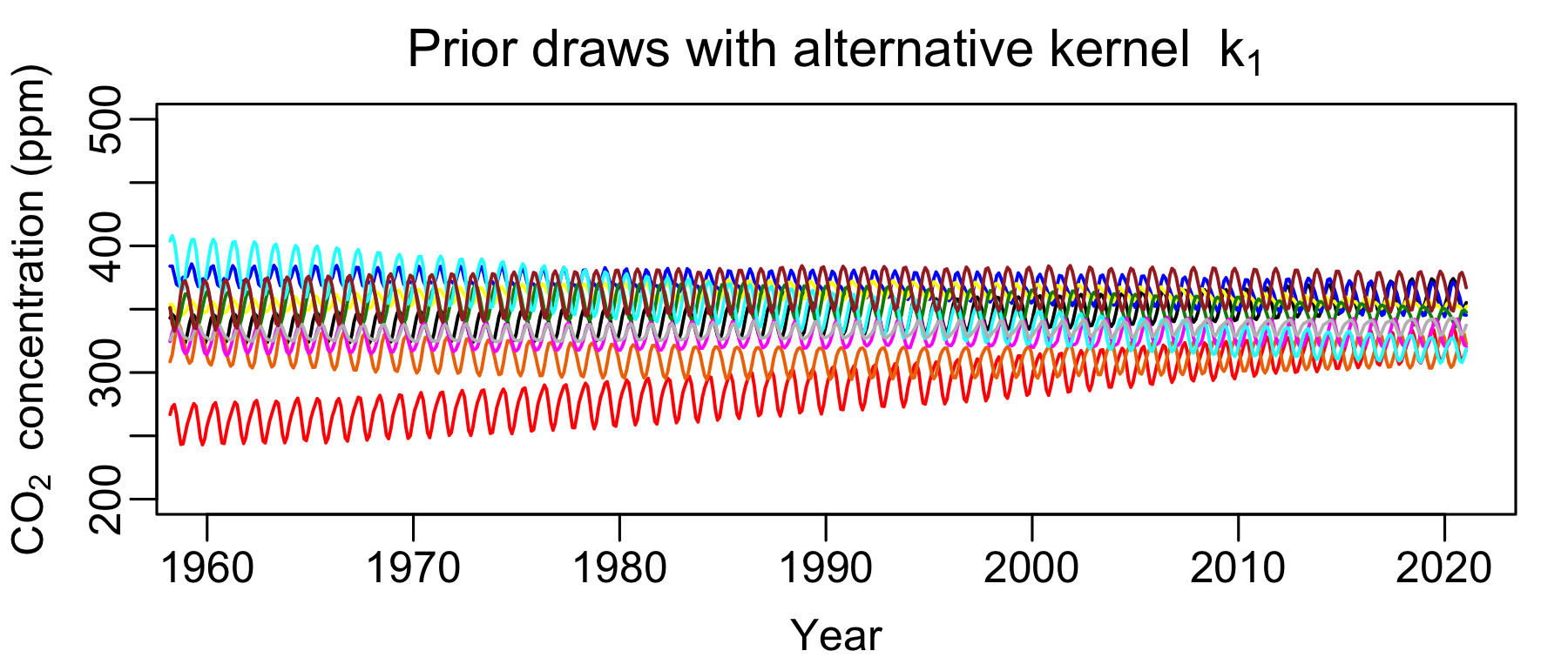
Robustness. We now use our workflow to ask whether qualitatively interchangeable kernels might have better predicted the record-breaking CO₂ levels in 2019; see Fig. 5 for our results. We lower the regularization strength (i.e. increase $\varepsilon$ in Algorithm 3) until $F^{\star}\geq L$. In the bottom of Fig. 5, we plot noise-matched prior draws from $k_{0}$ alongside draws from the resulting $k_{1}(\varepsilon^{*})$. Differences between draws from $k_{0}$ and $k_{1}(\varepsilon^{*})$ are almost visually indistinguishable on this scale. A closer inspection in Appendix D confirms that the two priors capture the same yearly periodic trend. These same zoomed-in plots show that the priors are not completely indistinguishable; however, in our opinion, the draws display the same prior beliefs. The 2-Wasserstein comparison in Fig. 16 of Appendix D further confirms that the perturbed kernel sits well within the histogram of alternate kernels stemming from hyperparameter uncertainty. We conclude that future predictions of CO₂ levels using the original $k_{0}$ are non-robust to the choice of kernel in the sense of Definition 1.

5 NON-STATIONARY PERTURBATIONS IN CLASSIFYING MNIST DIGITS

Figure 6: Sensitivity of MNIST analysis in Section 5. (Left): $F^{\star}$ as a function of regularizer strength. (Right): Histogram of the 2-Wasserstein distances between the $1000$ (one for each test image) input-warped kernel Gram matrices (in red) plotted with those arising from kernel hyperparameter uncertainty around $k_{0}$ (in black).

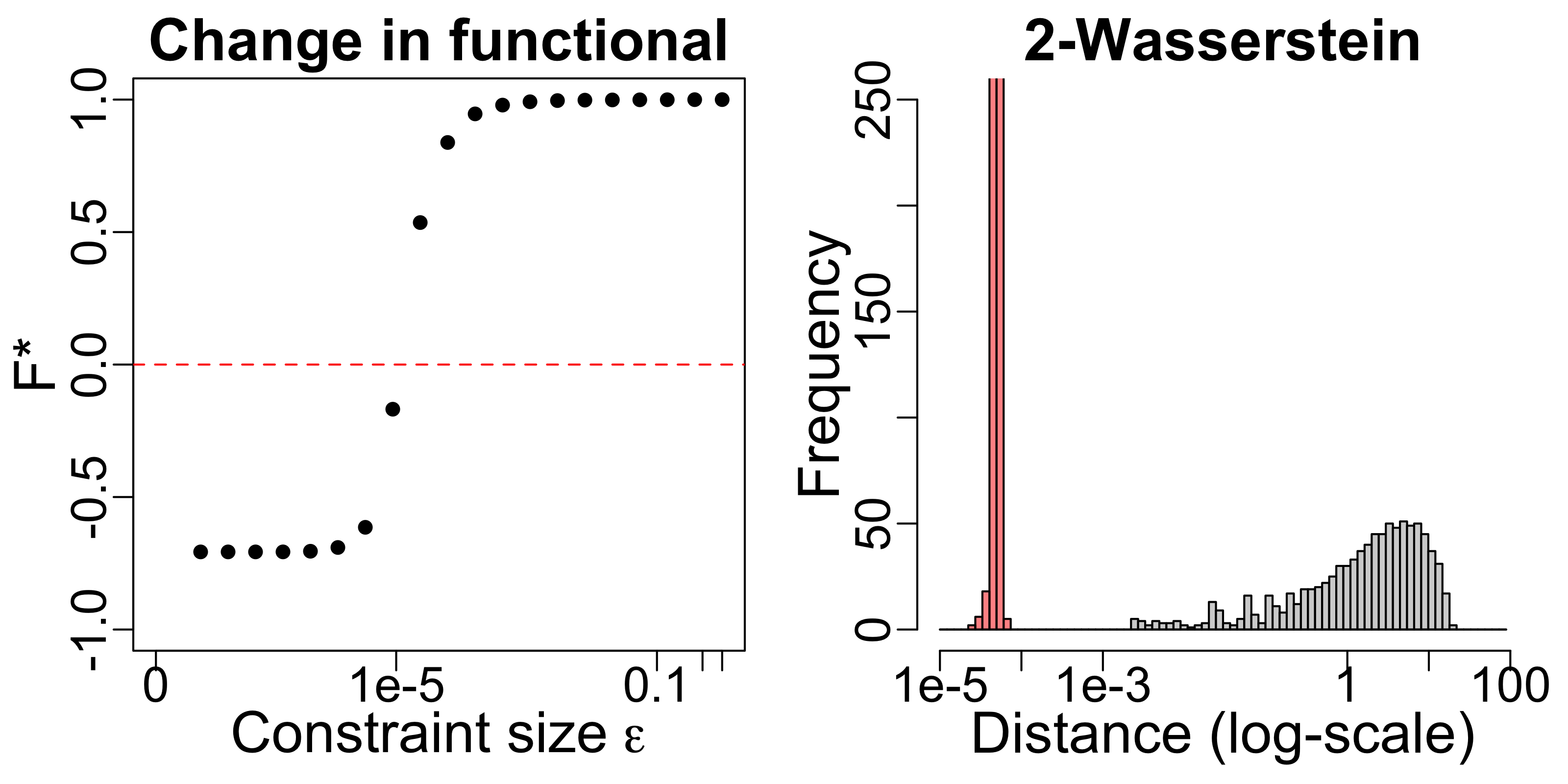
So far we have restricted our attention to low-dimensional covariates. To evaluate our approach in a high-dimensional setting, we reproduce the MNIST image classification experiment of Lee et al., (2018). It is rare to have specific beliefs about high-dimensional functions, so in this case we do not consider $k_{0}$ as arising from prior beliefs. Rather we imagine $k_{0}$ is used purely for convenience and predictive quality – but that a malicious actor is interested in changing the kernel to achieve different test predictions without detection.

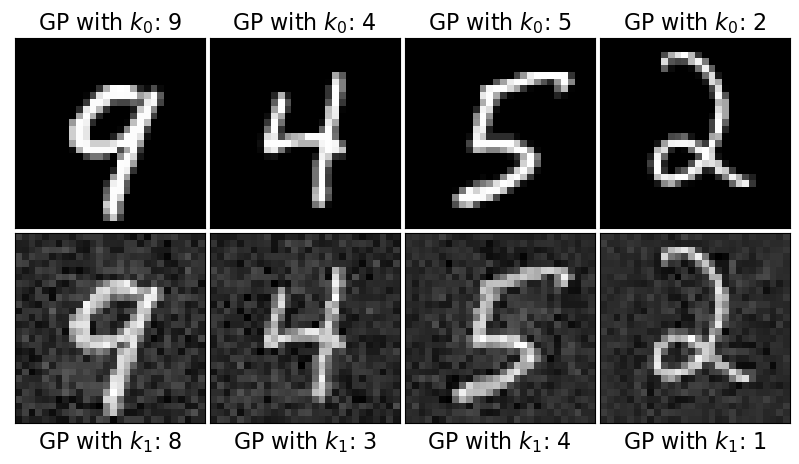
Data, model, and decision. Similar to Lee et al., (2018), we use 1000 randomly sampled MNIST images for a training set, and a separate 1000 images for a test set. Given a test image $\bm{x}^{\star}$, Lee et al., (2018) predict the class label $c\in\{1,\dots,C\}$ by using a $C$-output GP with compositional structure, considered as the infinite-width limit of a sequence of Bayesian neural networks (Lee et al.,, 2018; de G. Matthews et al.,, 2018). Let $f_{c}(\bm{x}^{\star})$ be the $c$th output. The authors classify any image $\bm{x}^{\star}$ by picking the class $c$ that has the posterior mean of $f_{c}(\bm{x}^{\star})$, i.e. $\mu_{c}(\bm{x}^{\star})$, closest to 0.9; see Appendix F for details. We use the kernel and hyperparameters from Lee et al., (2018) for $k_{0}$. We imagine that the malicious actor wants to change the label of a single test image $\bm{x}^{\star}$ from its current label $c_{0}$ to a different label $c_{1}$. For concreteness, we set $c_{1}:=|c_{0}-1|$. We consider 1000 separate iterations of this exercise, once for each of the 1000 test images. For a particular $\bm{x}^{\star}$, we set our posterior quantity of interest to be $F^{\star}=|\mu_{c_{0}}(\bm{x}^{\star})-0.9|-|\mu_{c_{1}}(\bm{x}^{\star})-0.9|$. Since $F^{\star}\geq 0$ implies that we have changed the prediction for $\bm{x}^{\star}$, we set our decision threshold $L=0$.

Malicious actor. Instead of considering a range of priors that match prior beliefs, we here consider a range of priors that will allow a malicious actor to avoid detection. Since we have no prior belief of stationarity, we use the non-stationary construction from Section 2.1. We find that optimizing $F^{\star}$ directly leads to kernels where for $c\neq c_{1}$, $\mu_{c}(\bm{x}^{\star})$ takes on values at least an order of magnitude higher than for the original kernel. This change could be easily detected by an automated system. For the purposes of the malicious actor, we therefore consider these kernels to not be qualitatively interchangeable. We instead optimize a surrogate loss that maximizes the log probability of $c_{1}$ being correct and all other classes being incorrect; see Appendix F. We find that optimizing this surrogate loss leads to more benign-looking $\mu_{c}(\bm{x}^{\star})$ and achieves $F^{\star}\geq L$.

Robustness. Fig. 6 shows the results of our workflow applied to this problem. We find a sufficiently large setting of $\varepsilon$ that allows us, across all 1000 test-image problems, to change every decision. In particular, for $\varepsilon=10^{-4},$ we are able to find perturbed kernels that change the predicted class label in every case. It is not clear how to visualize our priors in this application. So, of the approaches in Section 2.2, we use only the hyperparameter uncertainty visualization to assess qualitative interchangeability. Lee et al., (2018) optimize the hyperparameters of $k_{0}$ over a grid. Instead of bootstrapping this procedure, we note that the size of the grid defines a natural variability in the hyperparameters $\hat{\theta}$. To be conservative, we sample $\theta^{(r)}$ from an area around the hyperparameters selected by Lee et al., (2018) that is over 10 times smaller than the full grid. (Using the full original grid would find more extreme non-robustness.) The Gram matrices corresponding to our perturbed kernels are much closer to $k_{0}(X,X)$ than are the Gram matrices corresponding to each $\theta^{(r)}$. We conclude that classification of handwritten digits using $k_{0}$ is non-robust to the choice of kernel in the sense of Definition 1.

6 DISCUSSION

In this paper, we proposed and implemented a workflow for measuring the sensitivity of GP inferences to the choice of the kernel function. We used our workflow to discover substantial non-robustness in a variety of practical examples, but also showed that many analyses are not flagged as non-robust by our method. There are many exciting directions for expanding on the present work – both within our existing workflow and beyond. We discuss these directions below.

Improving our workflow. Our workflow is made up of many modular parts, and in some parts choices were made for mathematical convenience (e.g. the particular constraint in our stationary objective or the particular regularizer in our non-stationary objective in Algorithm 3). Perhaps different choices could be made to allow easier detection of non-robustness – or to allow for certification of robustness (whereas our workflow can only fail to find non-robustness)

What should we do about non-robustness? Our framework flags non-robustness but does not show how to make an analysis more robust. The instances of non-robustness we have found suggest it might be worthwhile to develop methods to robustify GP inferences to the choice of kernel. One challenge would be how to best balance robustness against the ability to adapt to the prior assumptions at hand: if a method is completely robust to any change in prior assumptions, there is no point in specifying a prior at all!

Studying model selection and robustness. Our example in Section 4 shows that the use of sophisticated kernel selection tools does not necessarily mean robustness issues are not present. However, it could be that non-robustness is typically lessened or removed by the use of such tools. Or maybe certain classes of kernel selection tools ameliorate non-robustness issues more than others. It remains to formalize and study these questions.

Acknowledgements

The authors thank Ryan Giordano for useful conversations about this work. This work was supported by the MIT-IBM Watson AI Lab, an NSF CAREER Award, an ARPA-E project with program director David Tew, and an ONR MURI.

Appendix A Details of spectral density constraints

Here, we give the details of how we optimize over spectral densities to produce a stationary kernel as summarized in Algorithm 2. Our goal is to optimize over the set of stationary kernels. It is not immediately clear how to enforce this constraint; however, Bochner’s theorem (Rasmussen and Williams,, 2006, Thm. 4.1) tells us that every stationary kernel $k(x,x^{\prime})=k(\tau)$, where $\tau=x-x^{\prime}$ has a positive finite spectral measure $\mu$ on $\mathbb{R}^{D}$ such that:

$$k(\tau)=\int_{\mathbb{R}^{D}}e^{2\pi i\tau^{T}\omega}d\mu(\omega).$$ (3)

A common assumption in the literature on kernel discovery (Wilson and Adams,, 2013; Benton et al.,, 2019; Wilson et al.,, 2016) is to assume that $\mu$ has a density $S$ with respect to the Lebesgue measure; that is, we can write:

$$k(\tau)=\int_{\mathbb{R}^{D}}e^{2\pi i\tau^{T}\omega}S(\omega)d\omega.$$ (4)

These works have shown that the class of stationary kernel with spectral densities is a rich, flexible class of kernels. We thus focus on the class of stationary kernels with spectral densities as this allows us to transform the problem of optimizing over stationary kernels into the problem of optimizing over positive real valued functions. In all of our examples optimizing over spectral densities, we have $D=1$. We thus assume $D=1$ in the rest of our development here. In this case, it must be that $S$ is symmetric around the origin to obtain a real-valued $k$. So, we can simply Eq. 4 further as:

$$k(\tau)=\int_{0}^{\infty}\cos(2\pi\tau\omega)S(\omega)d\omega.$$ (5)

Optimizing over positive functions $S$ on the positive real line seems at least somewhat more tractable than optimizing over stationary positive-definite functions $k(\tau)$. However, this is still an infinite dimensional optimization problem. To recover a finite dimensional optimization problem, we follow Benton et al., (2019) and choose a grid $\omega_{1},\dots,\omega_{G}$. We can then optimize over the finite values $S(\omega_{1}),\dots,S(\omega_{G})$ and use the trapezoidal rule to approximate the integral in Eq. 5. Benton et al., (2019) find that $G=100$ gives reasonable performance in their experiments; we find the same in ours, and fix $G=100$ throughout. Benton et al., (2019) recommend setting $\omega_{g}=2\pi g/(8\tau_{max})$, where $\tau_{max}$ is the maximum spacing between datapoints. We find this to sometimes give inaccurate results in the sense that using the trapezoidal rule / an exact formula to compute the density of $k_{0}$, $S(\omega_{1}),\dots,S(\omega_{G})$ and then using the trapezoidal rule to recover the gram matrix $k_{0}(X,X)$ gives an inaccurate approximation to $k_{0}(X,X)$. This is problematic in our case, as it would imply $k_{0}(X,X)$ is not in the constraint set for small $\varepsilon$. Instead, we recommend setting our $\omega_{g}$’s as a uniform grid from $\omega_{1}=0$ up to an $\omega_{G}$ such that $S_{0}(\omega_{G})$ is equal to the floating point epsilon ($10^{-15}$ in our experiments); some manual experimentation will be required to implement this rule.

As we are only interested in kernels nearby $k_{0}$, we will have to put some kind of constraint on $k_{1}$’s spectral density, $S_{1}(\omega_{1}),\dots,S_{1}(\omega_{G})$. We use a simple $\varepsilon$-ball given by:

$$\max\big{(}0,(1-\varepsilon)S_{0}(\omega_{g})\big{)}\leq S_{1}(\omega_{g})\leq(1+\varepsilon)S_{0}(\omega_{g}),\quad g=1,\dots,G,$$ (6)

Because our posterior functional of interest $F^{\star}$ is a differentiable function of the kernel matrix, we can compute gradients of $F^{\star}$ with respect to our discretized spectral density. Rather than manually work out the derivatives of the trapezoidal rule combined with $F^{\star}$, we use the automatic differentiation package jax (Bradbury et al.,, 2018). Given a gradient of $F^{\star}$, we take a step in the direction of the gradient and then project the current iterate onto our constraint set in Eq. 6 by clipping the resulting spectral density.

Appendix B Additional details of synthetic-data experiment

We generated the $x$-component of the synthetic data by first drawing $25$ uniform random numbers in $[0,5].$ To investigate what happens when interpolating in a region of dense training data, we then add $3.00,3.025,3.075$, and $3.10$ as covariates (recall the interpolation point is $\bm{x}^{\star}=3.05$). The extrapolation point $\bm{x}^{\star}=5.29$ lies $0.5$ to the right of the largest $x$ value drawn. The $y$-component is defined to be, $y_{n}=x_{n}+\epsilon_{n}$, where $\epsilon_{n}\stackrel{{\scriptstyle iid}}{{\sim}}\mathcal{N}(0,1.5)$.

To discretize the spectral density, we follow Appendix A in using $100$ frequencies evenly-spaced from $0$ to $3.5.$ To optimize over nearby spectral densities, we also perform constrained gradient descent with randomized initializations in the sense of Appendix A. For extrapolation ($\bm{x}^{\star}=5.29$), using $25$ random seeds, we find non-robustness. For interpolation ($\bm{x}^{\star}=3.05$), even with $40$ random seeds, we do not find non-robustness.

Fig. 13 compares the distance between $k_{1}$ and $k_{0}$ to the distances between $k_{0}$ and $k^{(r)},$ where $k^{(r)}$ is a bootstrapped version of $k_{0}.$

Computation for the synthetic experiments is done using a computing cluster, which has xeon-p8 computing cores. We request $7$ nodes, each using $15$ cores to run parallel experiments across both $\epsilon$ and the random seed for initialization. Total wall-clock time comes to roughly $10$ minutes.

Appendix C Additional details for the heart rate example

Figure 7: Sensitivity of heart rate analysis in Appendix C for an example where we do not find non-robustness. (Top-left): Heart rate data; notice the data is trending downwards at the end of the time series. (Top-right): Prior draws from our original kernel $k_{0}$ from Eq. 7). (Bottom-left): Prior draws from our decision-changing kernel $k_{1}$ that achieves $F^{\star}=L$, noise matched by color to the draws from $k_{0}$. (Bottom-right): Comparison of the difference between $k_{0}$ and $k_{1}$ (red line) to posterior hyperparameter uncertainty (histogram).

Here, we give additional details for our heart rate modeling example from Section 3. According to Reyna et al., (2019), the data was collected under the approval of appropriate institutional review boards, and personal identifiers were removed. Following Colopy et al., (2016), we first take the log transform of our heart rate observations $y_{n}$. We then zero-mean the observations ($\sum_{n=1}^{N}y_{n}=0$) and set them to have unit variance ($\sum_{n=1}^{N}y_{n}^{2}=1$). The kernel used by Colopy et al., (2016) to model the resulting data log-scaled standardized data is a Matérn $5/2$ kernel plus a squared exponential kernel:

$$k_{0}(x,x^{\prime})=h_{1}^{2}\left(1+\frac{\sqrt{5}\left|x-x^{\prime}\right|}{\lambda_{1}}+\frac{5\left|x-x^{\prime}\right|^{2}}{3\lambda_{1}}\right)\exp\left[-\frac{\sqrt{5}\left|x-x^{\prime}\right|}{\lambda_{1}}\right]+h_{2}^{2}\exp\left[-\frac{\left|x-x^{\prime}\right|^{2}}{2\lambda_{2}^{2}}\right],$$ (7)

where $h_{1},h_{2},\lambda_{1},\lambda_{2}>0$ are kernel hyperparameters, which we set via MMLE. While all inferences are done on the zero-mean, unit-variance log-scaled data, all of our plots and discussion are given in the untransformed (i.e. raw bpm) scale for ease of interpretability.

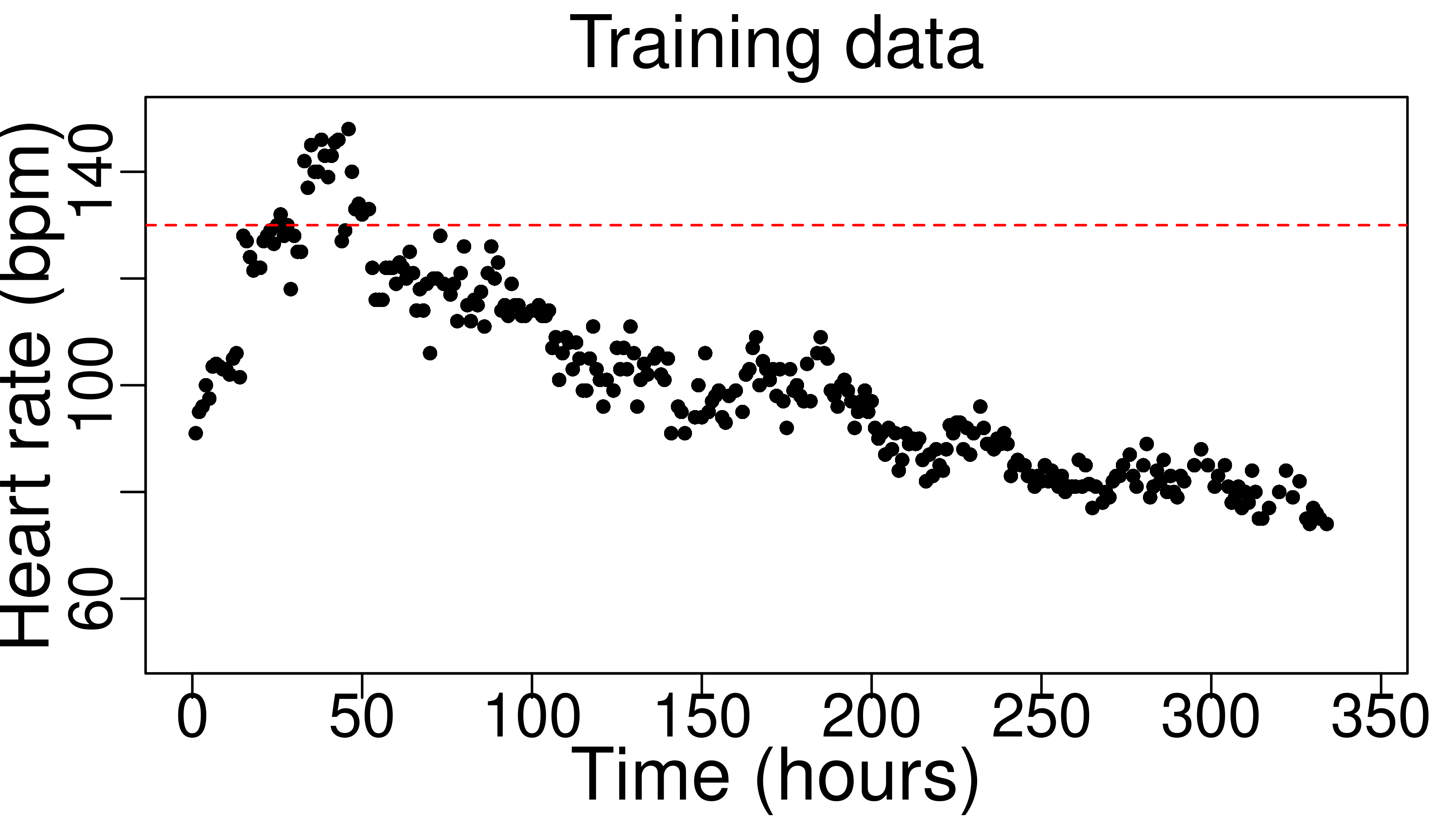
In the main text, we showed an example where our workflow in Algorithm 1 discovered non-robustness in predicting whether a patient’s heart rate would be likely to be above 130 BPM or not 1.5 hours in the future. We noted that there was some evidence in the data supporting this finding: the patient’s heart rate was trending upward towards the end of the observed data, so we might expect that small changes to the prior could result in significant posterior mass being placed on high heart rates. To demonstrate that we do not always find GP analyses non-robust to the choice of the prior, we give an example here where we do not find non-robustness. For our example, we use a different patient from the Computing in Cardiology challenge Reyna et al., (2019); Goldberger et al., (2000). The heart rate for this patient is plotted in Fig. 7; notice that their heart rate is trending down at the end of the observed data.

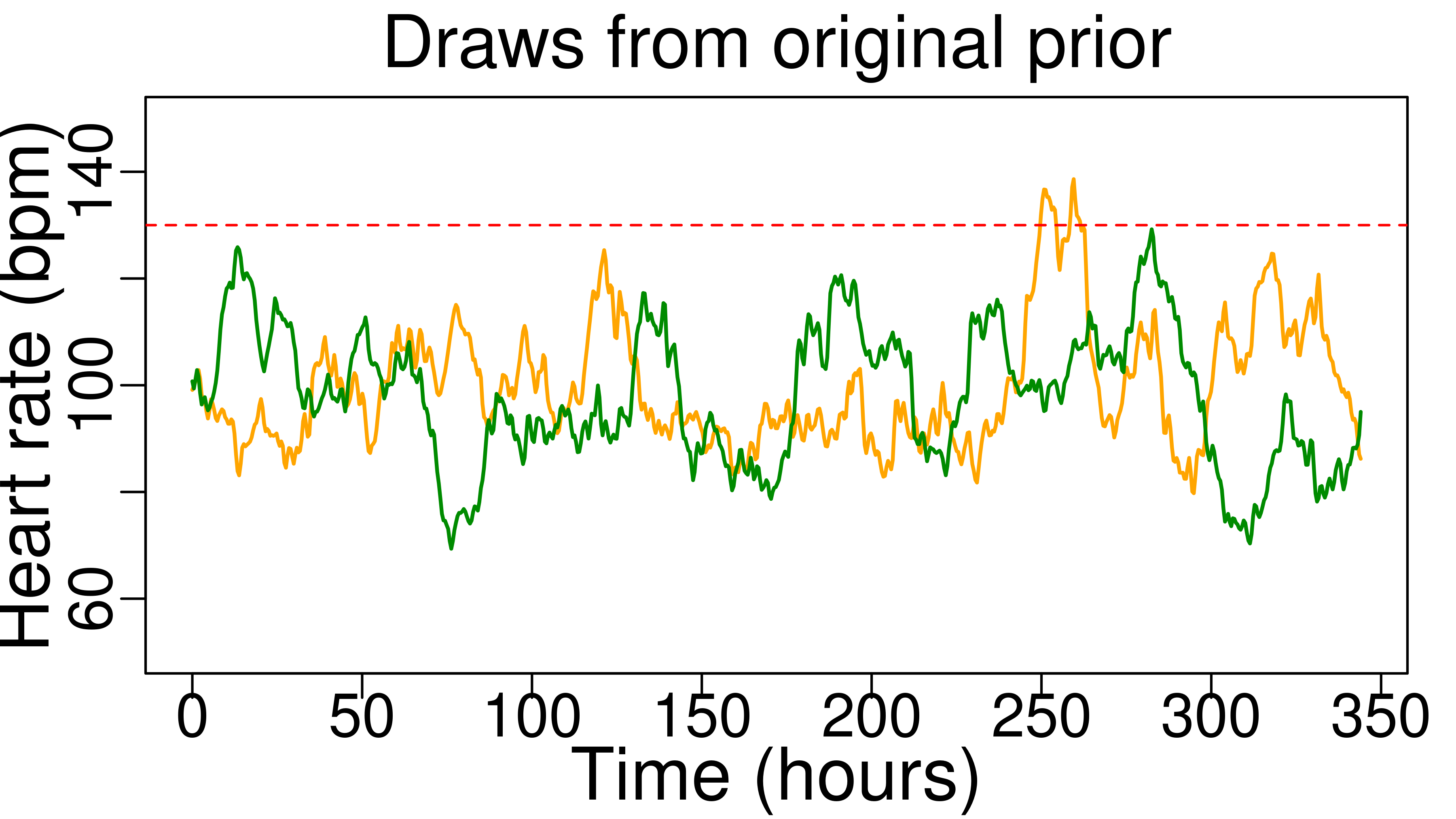
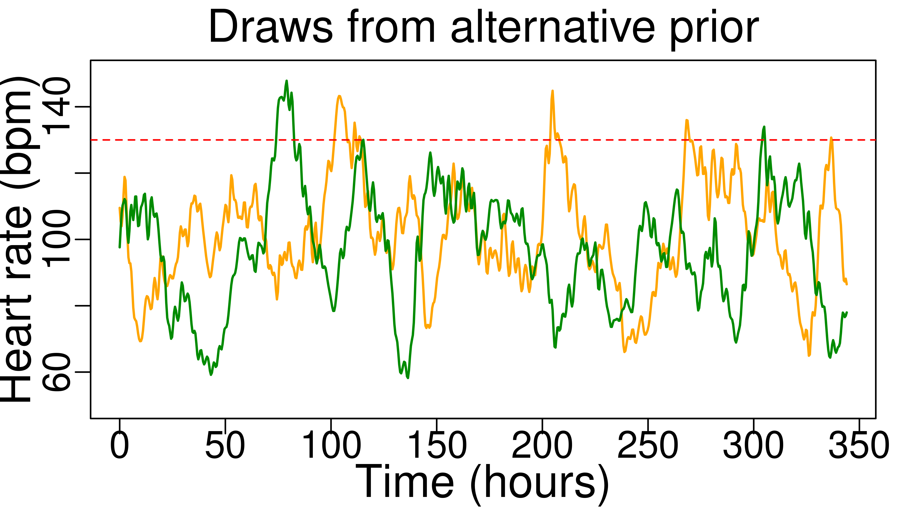
As in Section 3, we use the constraint set and objective specified by Algorithm 2 (i.e. we constrain ourselves to stationary kernels with spectral densities close to the density of $k_{0}$). Following Algorithm 1, we solve Eq. 2 to find $k_{1}(\varepsilon^{*})$ such that $F^{\star}(k_{1}(\varepsilon^{*}))=L$. We then assess whether the recovered $k_{1}(\varepsilon^{*})$ is qualitatively qualitatively interchangeable with $k_{0}$. We plot noise-matched prior draws from $k_{0}$ and $k_{1}(\varepsilon^{*})$ in Fig. 7. We see that $k_{1}(\varepsilon^{*})$ has obvious qualitative deviations from $k_{0}$; the functions drawn from $k_{1}(\varepsilon^{*})$ have noticably larger variance (count the number of times the functions from $k_{1}(\varepsilon^{*})$ pass 130 bpm). Additionally, we see in Fig. 7 that the 2-Wasserstein distance between $k_{0}(X,X)$ and $k_{1}(X,X)$ is much larger than the typical deviations around $k_{0}$ due to hyperparameter uncertainty. We conclude that $k_{0}$ and $k_{1}(\varepsilon^{*})$ are not qualitatively interchangeable. Thus, we say that we do not find non-robustness in the sense of Definition 1. Again, this conclusion is fairly sensible: at the final observation, the patient’s heart rate is below 80 BPM and is trending downwards. It thus seems reasonable that it would take a somewhat unusual prior to predict that the patient’s heart rate would suddenly spike to 130.

The two heart rate experiments in were run on a laptop with a six-core i7-9750H processor. The experiments took roughly five minutes each to complete.

Appendix D Additional details for CO₂ experiment

Figure 8: Sensitivity analysis of Mauna Loa. Each plot shows noise matched samples from a zero mean Gaussian process with original and perturbed kernel functions. These plots provide a zoomed in view of the prior samples shown in Fig. 5. We note that draws from $k_{1}(\varepsilon^{*})$ are in-phase with those of $k_{0}$ (i.e. $k_{1}(\varepsilon^{*})$ captures the seasonal maxima and minima of CO₂ just as well as $k_{0}$ does). Overall, there is high agreement between functions sampled from the two GPs.

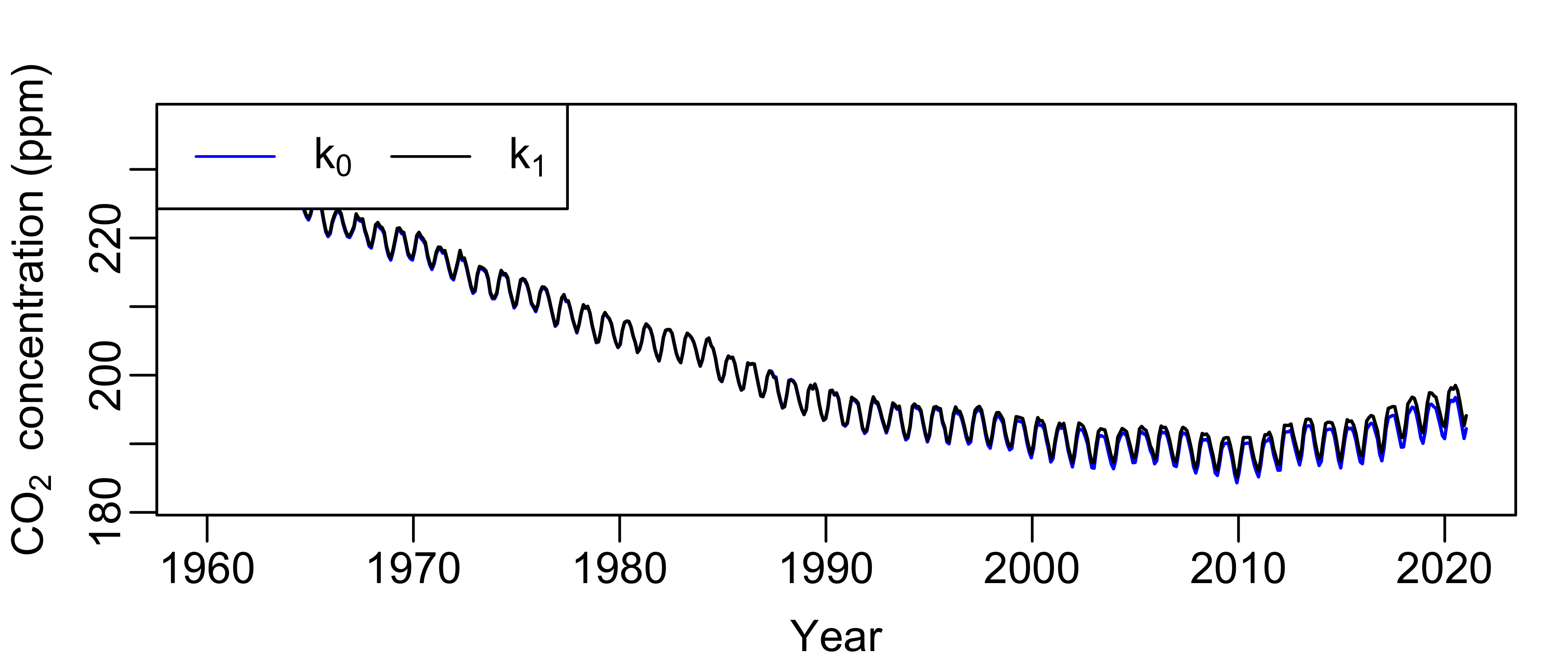
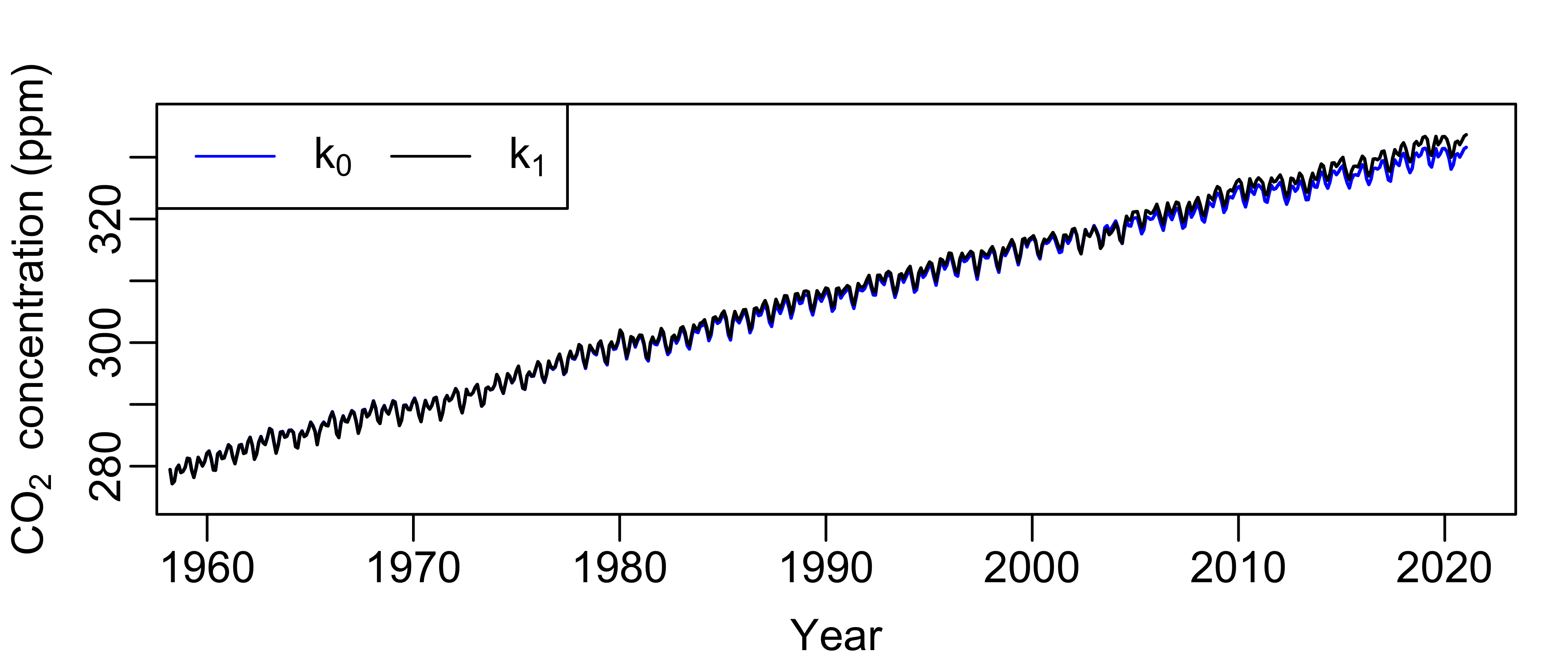
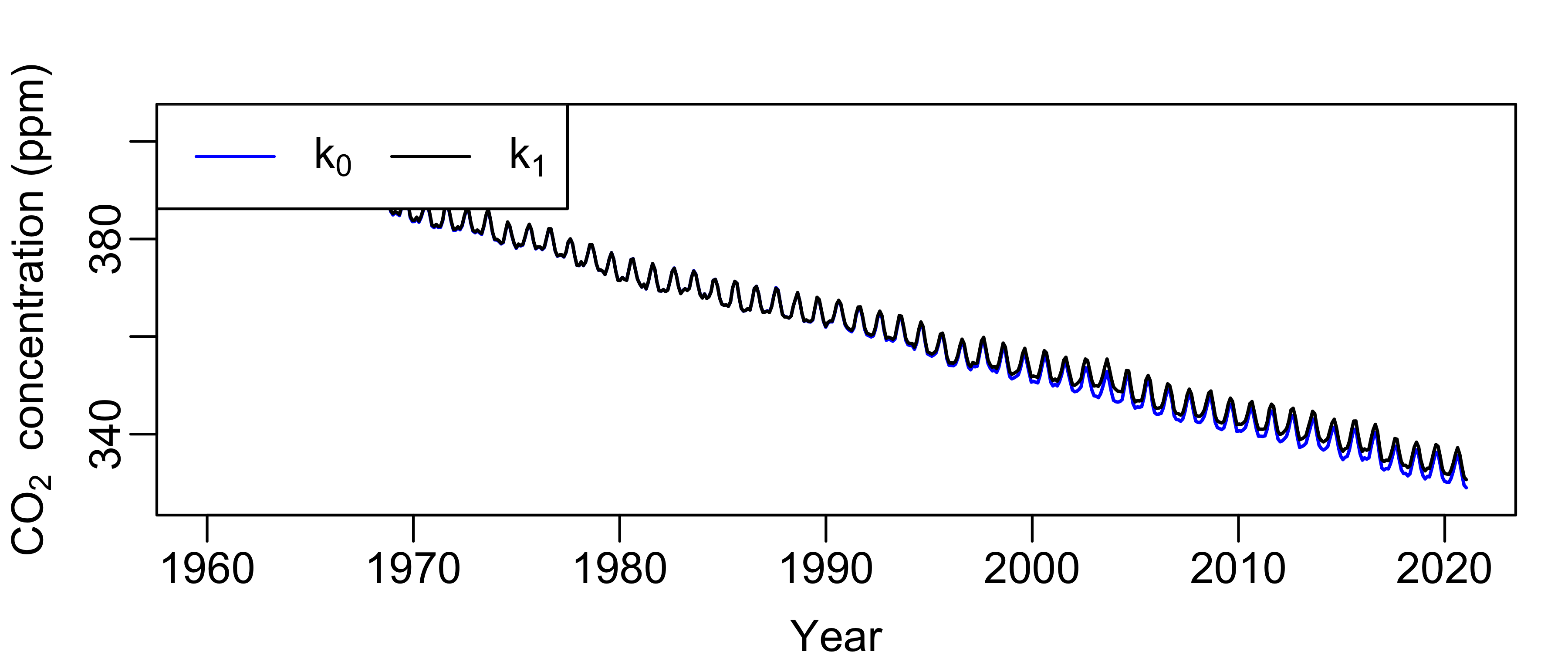
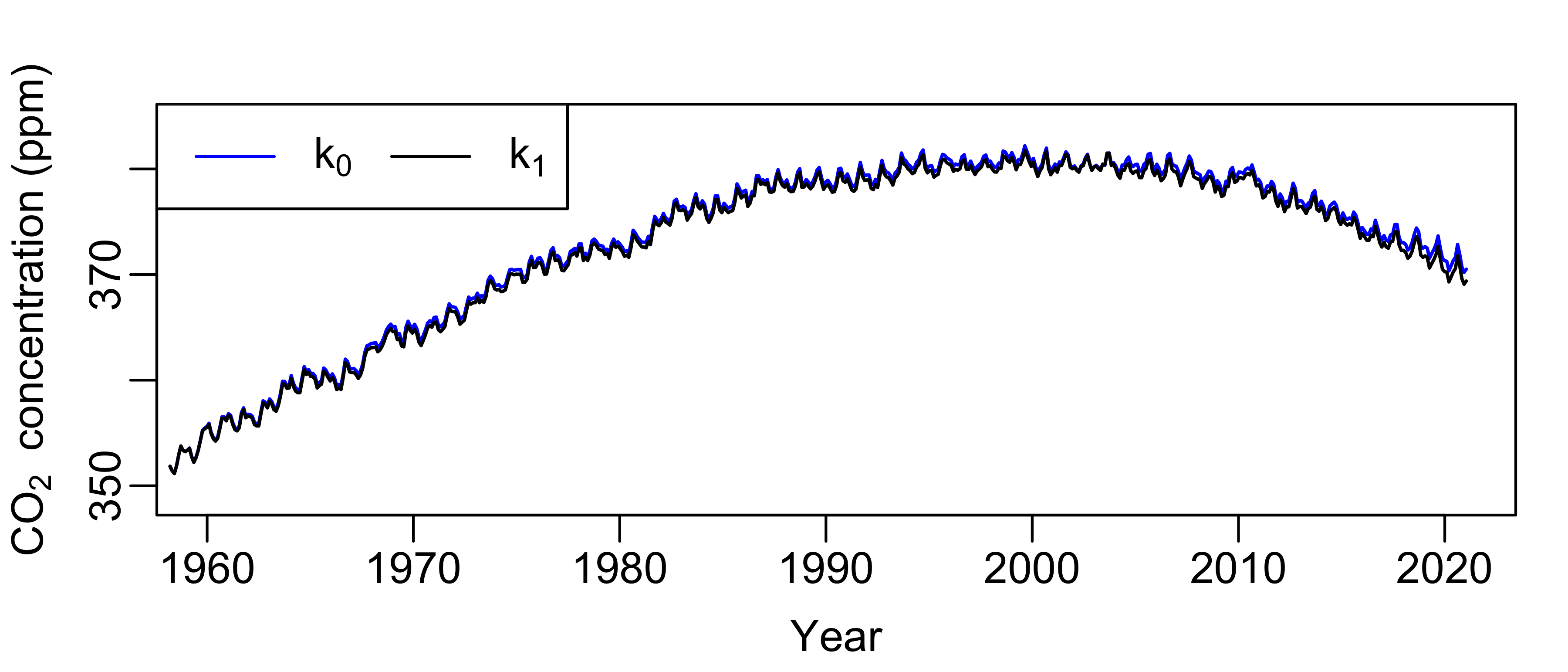
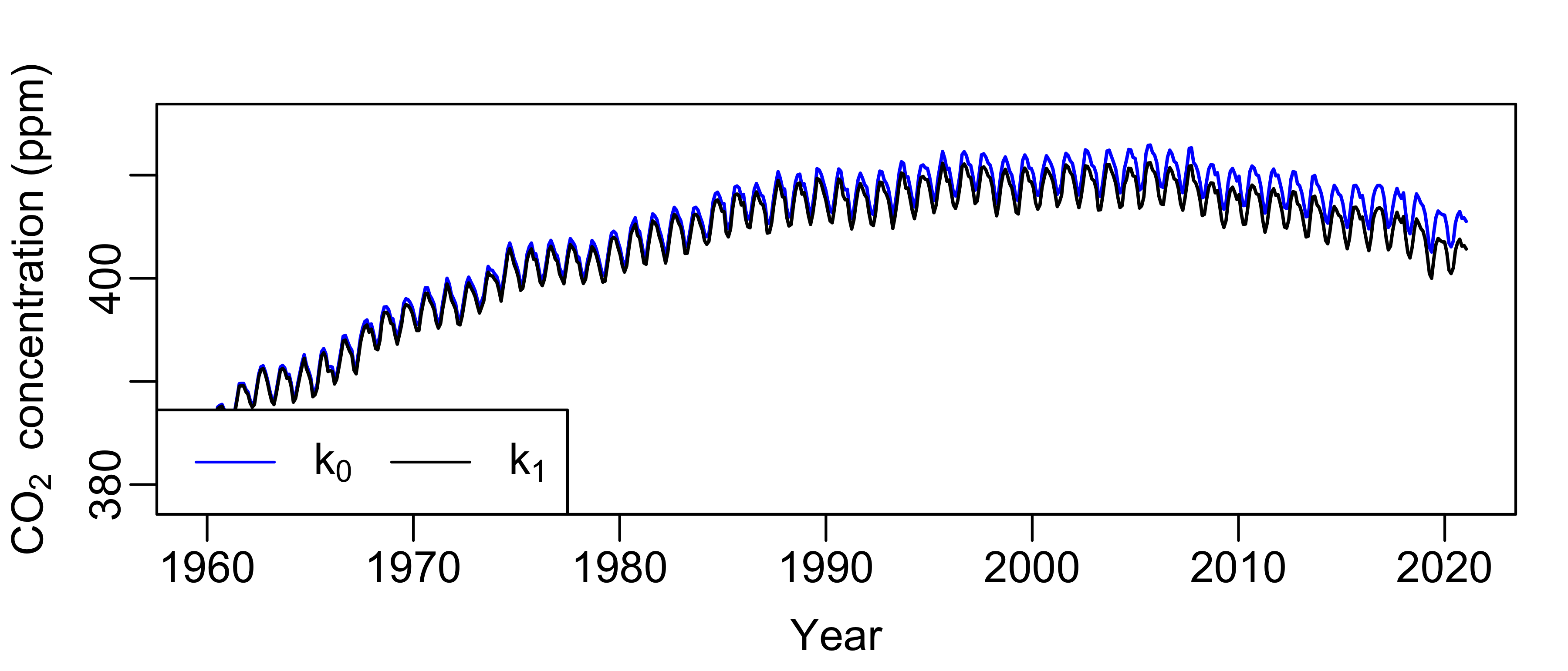
Here, we give additional details on the CO₂ experiment from Section 4. Our dataset is a series of monthly CO₂ levels taken from Mauna Loa in Hawaii between 1958 and 2021 (Keeling et al.,, 2005); we download our data from https://scrippsco2.ucsd.edu/assets/data/atmospheric/stations/in_situ_co2/monthly/monthly_in_situ_co2_mlo.csv. Rasmussen and Williams, (2006, Section 5.4.3) predict future CO₂ levels using a GP. Their kernel is the sum of four terms:

$$k_{0}(x_{1},x_{2}) =\theta_{1}^{2}\exp\left(-\frac{(x_{1}-x_{2})^{2}}{2\theta_{2}^{2}}\right)$$ (8)

$$+\theta_{3}^{2}\exp\left(-\frac{(x_{1}-x_{2})^{2}}{2\theta_{4}^{2}}-\frac{2\sin^{2}(\pi(x_{1}-x_{2}))}{\theta_{5}^{2}}\right)$$ (9)

$$+\theta_{6}^{2}\left(1+\frac{(x_{1}-x_{2})^{2}}{2\theta_{7}^{2}\theta_{8}}\right)^{-\theta_{8}}$$ (10)

$$+\theta_{9}^{2}\exp\left(-\frac{(x_{1}-x_{2})^{2})}{2\theta_{10}^{2}}\right),$$ (11)

where the $\theta_{i}$ comprise the kernel hyperparameters (in addition to the noise variance $\sigma^{2}$). The different components of this kernel encode different pieces of prior knowledge. The two squared exponentials encode long-term trends and small-scale noise, respectively. The rational quadratic kernel (Eq. 14) encodes small seasonal variability in CO₂ levels between different years. The periodic kernel captures the periodic trend in CO₂ levels, which peak in the summer and reach their minimum in the winter. This periodic is multiplied by a squared exponential to allow deviations away from exact periodicity.

Similar to (Rasmussen and Williams,, 2006, Section 5.4.3), we first transform the training data by making the CO₂ levels have zero mean. To set the GP hyperparameters, we find that the hyperparameters values reported in Rasmussen and Williams, (2006, Section 5.4.3) are close, but not exactly, the MMLE solution on our data set (the gradient of the marginal log-likelihood has an entry substantively different from zero under the parameters from Rasmussen and Williams, (2006)). We set hyperparameters by $10$ random restarts of MMLE, where the solution iterates are initialized at the values reported in (Rasmussen and Williams,, 2006, Section 5.4.3). The fitted values are $\theta_{1}=68.58$, $\theta_{2}=69.09$, $\theta_{3}=2.55$, $\theta_{4}=87.60$, $\theta_{5}=1.44$, $\theta_{6}=0.66$, $\theta_{7}=1.18$, $\theta_{8}=0.74$, $\theta_{9}=0.18$, $\theta_{10}=0.13$, $\theta_{11}=0.19.$ They are, for the most part, within $5\%$ of the values reported in Rasmussen and Williams, (2006, Section 5.4.3).

When Rasmussen and Williams, (2006) ran their analysis, only data up to 2003 were available. As it turns out, their analysis significantly underestimates current CO₂ levels. In particular, they fail to predict the fact that CO₂ levels hit 415 ppm for the first time in human history in 2019; in fact, the maximum of the predicted CO₂ levels in 2019 is over three posterior standard deviations away from 415 ppm. We ask if a qualitatively interchangeable kernel could have changed this result. Ideally, we would set $F^{\star}$ to be the max of all posterior predictions in 2019. However, this is not a smooth function of the kernel. So we instead let $F^{\star}$ to be the smooth max of the posterior means of all the test points in 2019, $\{\mu(x_{t})\}_{t=1}^{T}$. The smooth-max we use is a scaled log-sum-exp, with a scale $\alpha>0$: $F^{\star}(k)=\log\left(\sum_{t=1}^{T}e^{\alpha\mu(x_{t})}\right)/\alpha.$ Larger values of $\alpha$ provide a better approximation to the actual max function but may cause numerical difficulties; we choose $\alpha=10$ as it seems to provide a reasonable approximation to the max function without introducing numerical problems. While we optimize using this approximation to the max, our experiments show that the recovered $k_{1}(\varepsilon^{*})$ have an exact max prediction in 2019 of 415 ppm.

$k_{0}$ is stationary, so we could search for alternative stationary kernels using our spectral density framework from Section 2.1 (Algorithm 2). However, there is good reason to think we might want to consider non-stationary prior beliefs. Developments in technology and/or global policy could have a large impact on CO₂ levels. Thus, we might encode past / expected future changes in technology and policy into our prior beliefs, making our prior beliefs non-stationary.

Thus, we use the input warping approach from Section 2.1 (Algorithm 3). However, we do not input warp the entirety of $k_{0}$. As we know CO₂ data has a regular periodicity, we leave the periodic component of the kernel, $\exp[-2\sin^{2}(\pi(x_{1}-x_{2}))/\theta^{2}_{5}]$ unwarped. In preliminary experiments, we input warped the entirety of $k_{0}$; the resulting prior draws sometimes had minima in the summer and maxima in the winter, a clear violation of our prior knowledge about CO₂ levels. We input warp all other parts of $k_{0}$ using a use a two hidden layer fully connected network, with $50$ units and ReLU nonlinearities to parameterize $h$. Finally, to ensure the optimal $k_{1}(\varepsilon)$ is finite, we use $\ell(k;F^{\star},L)=(F^{\star}(k)-L)^{2}$ in Algorithm 3, which guarantees that our objective is bounded below.

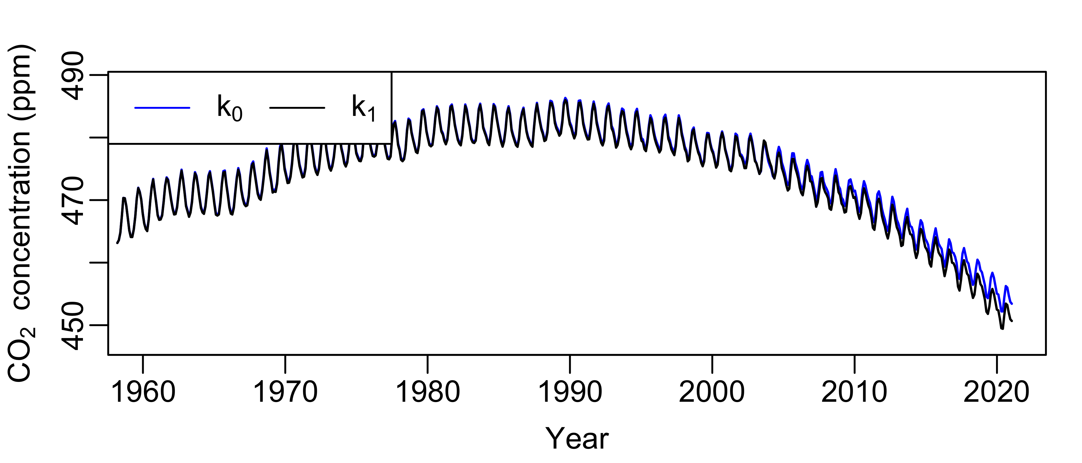
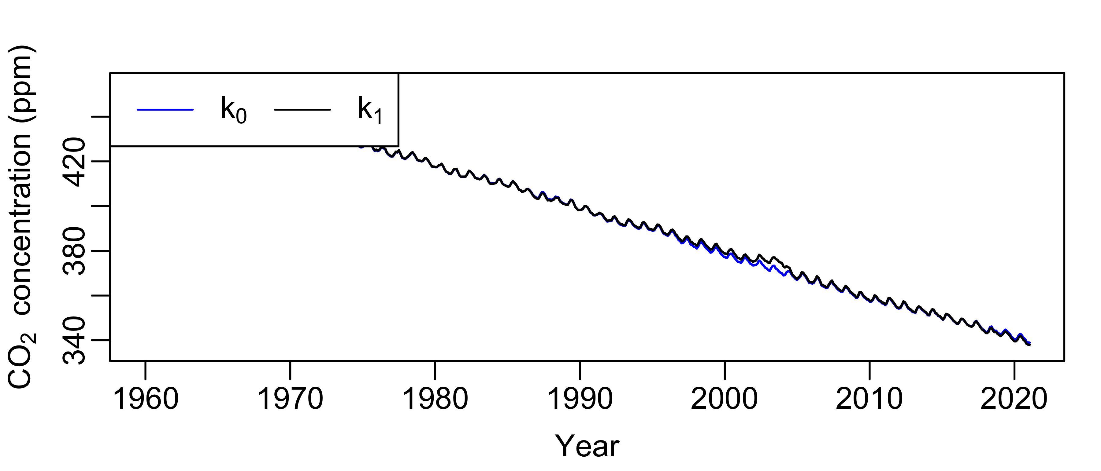
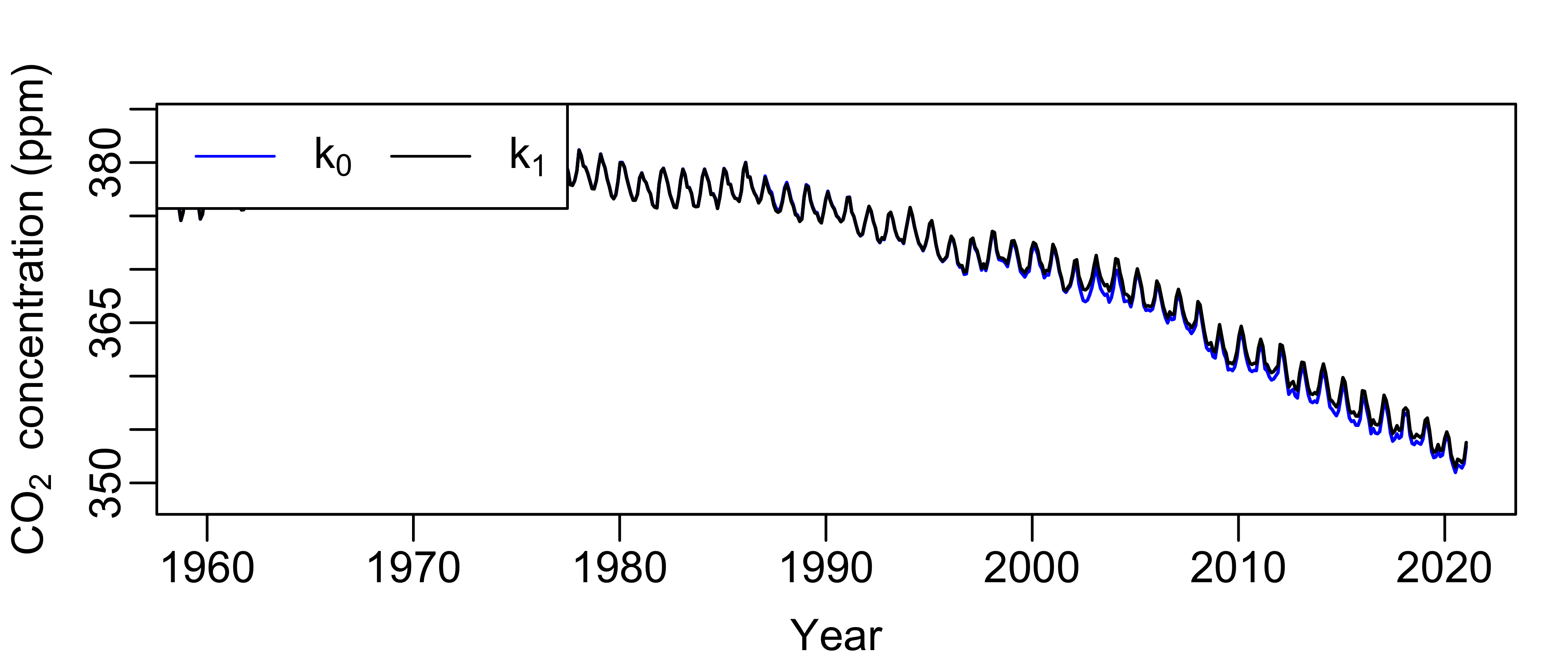
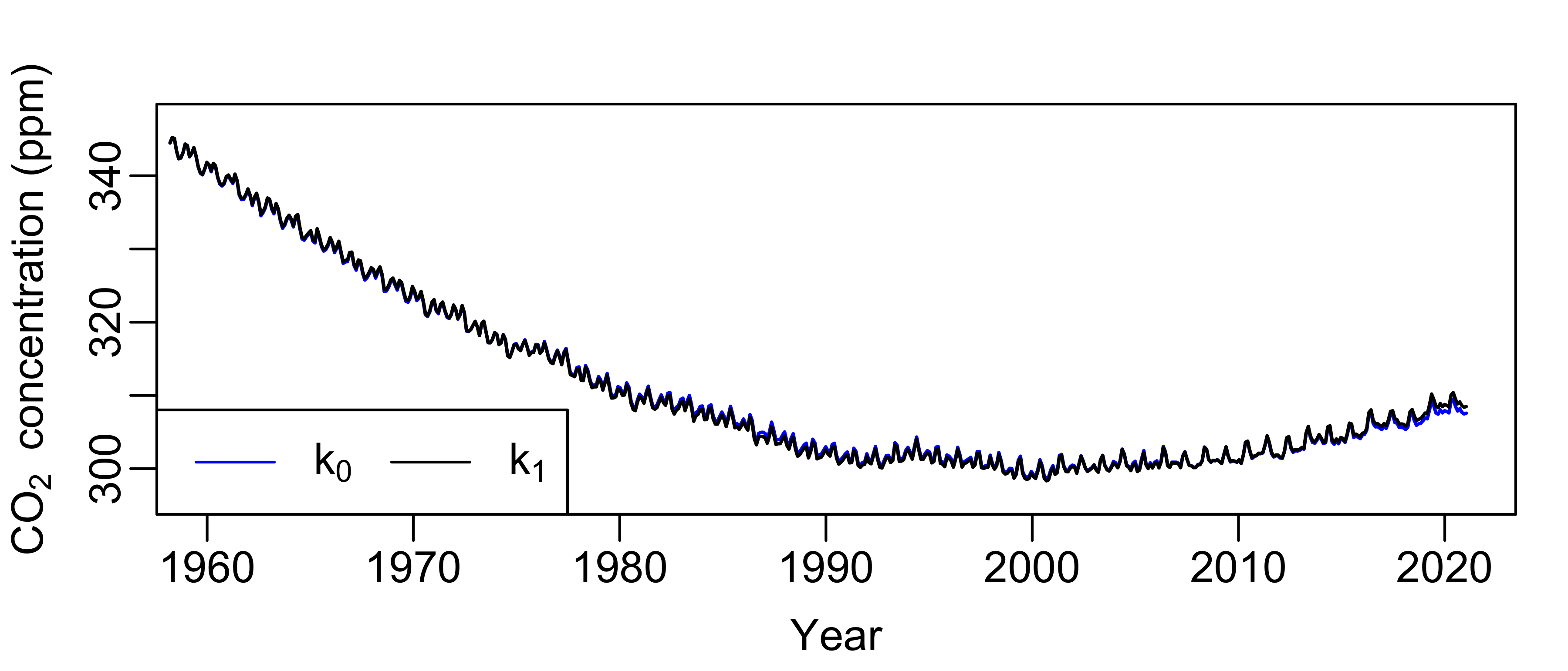
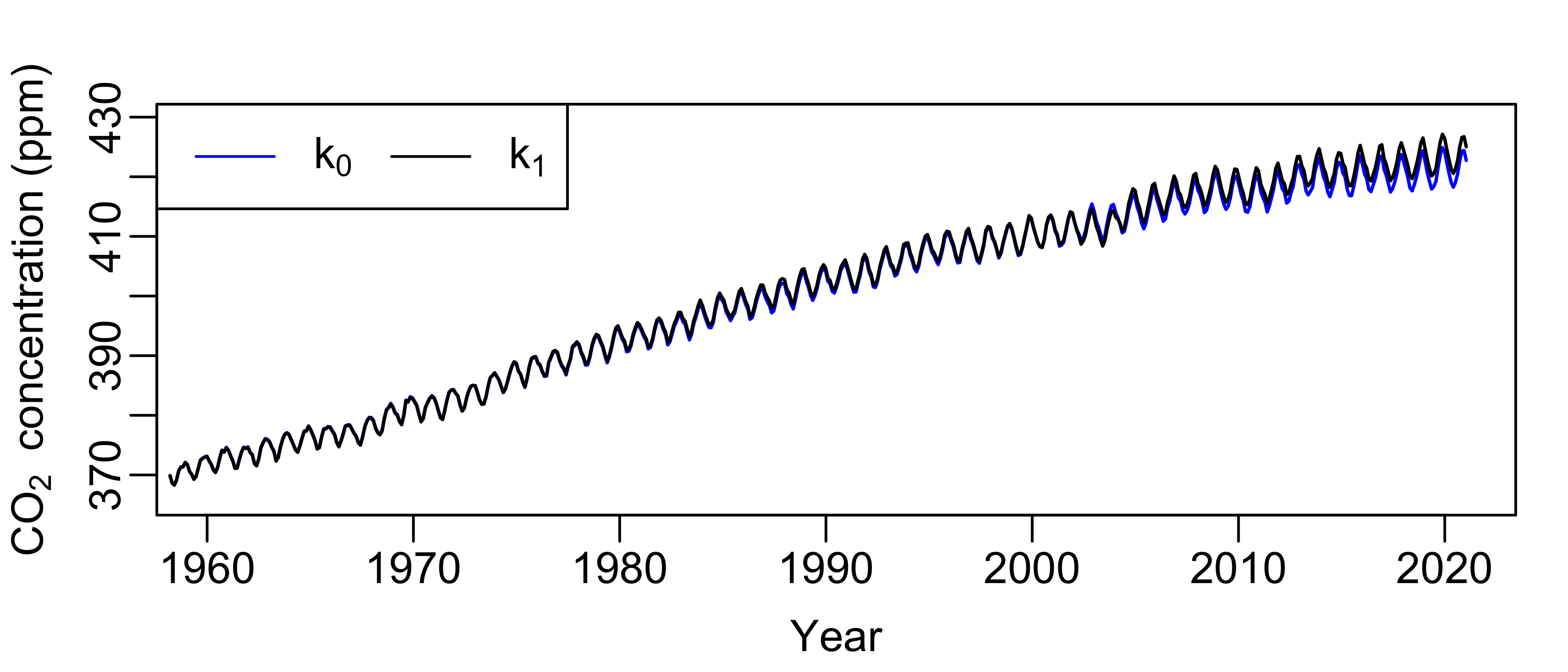
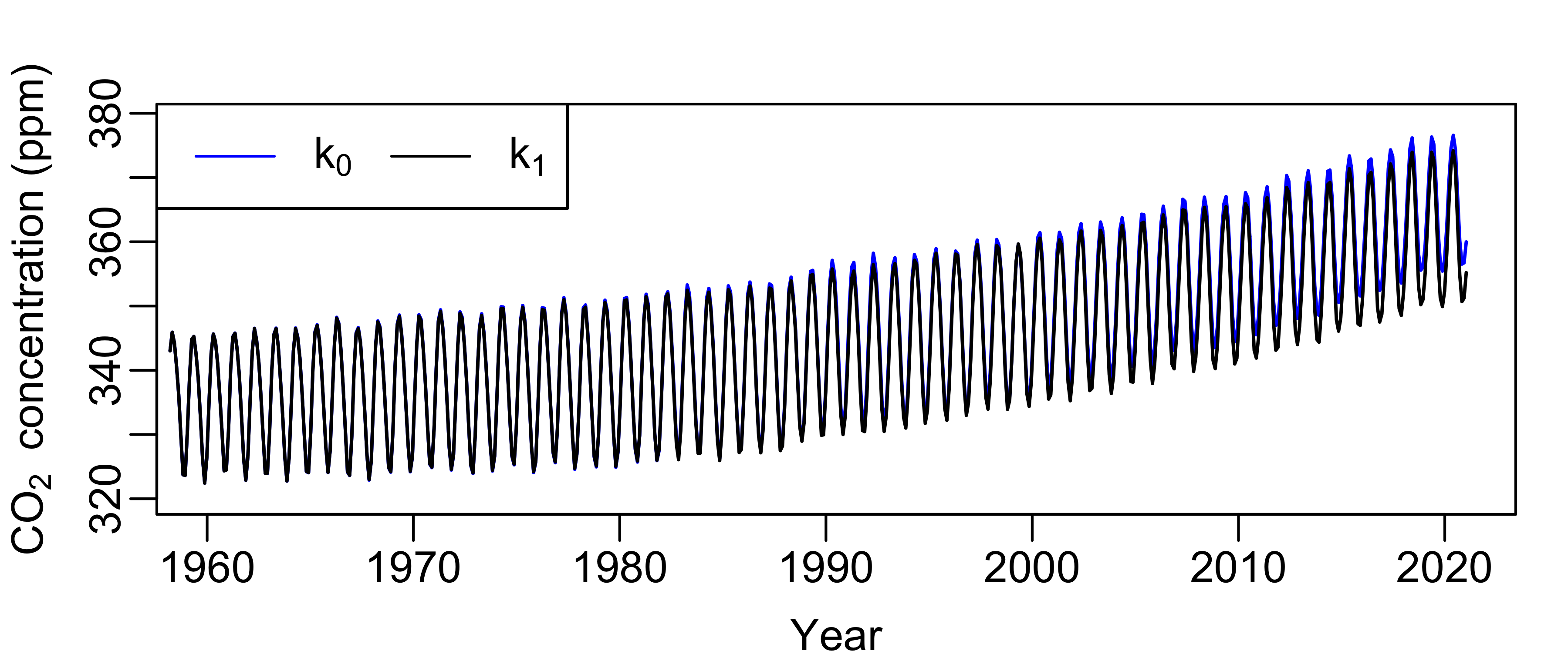
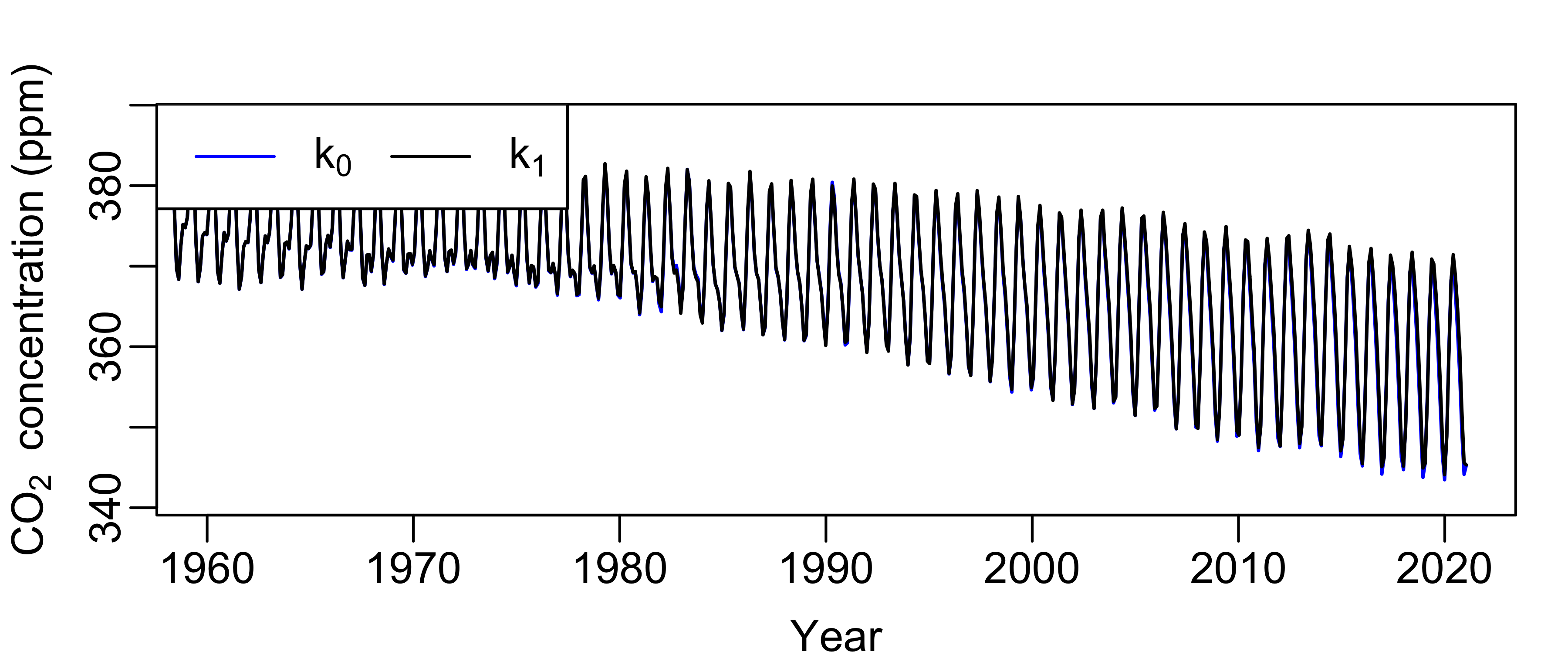
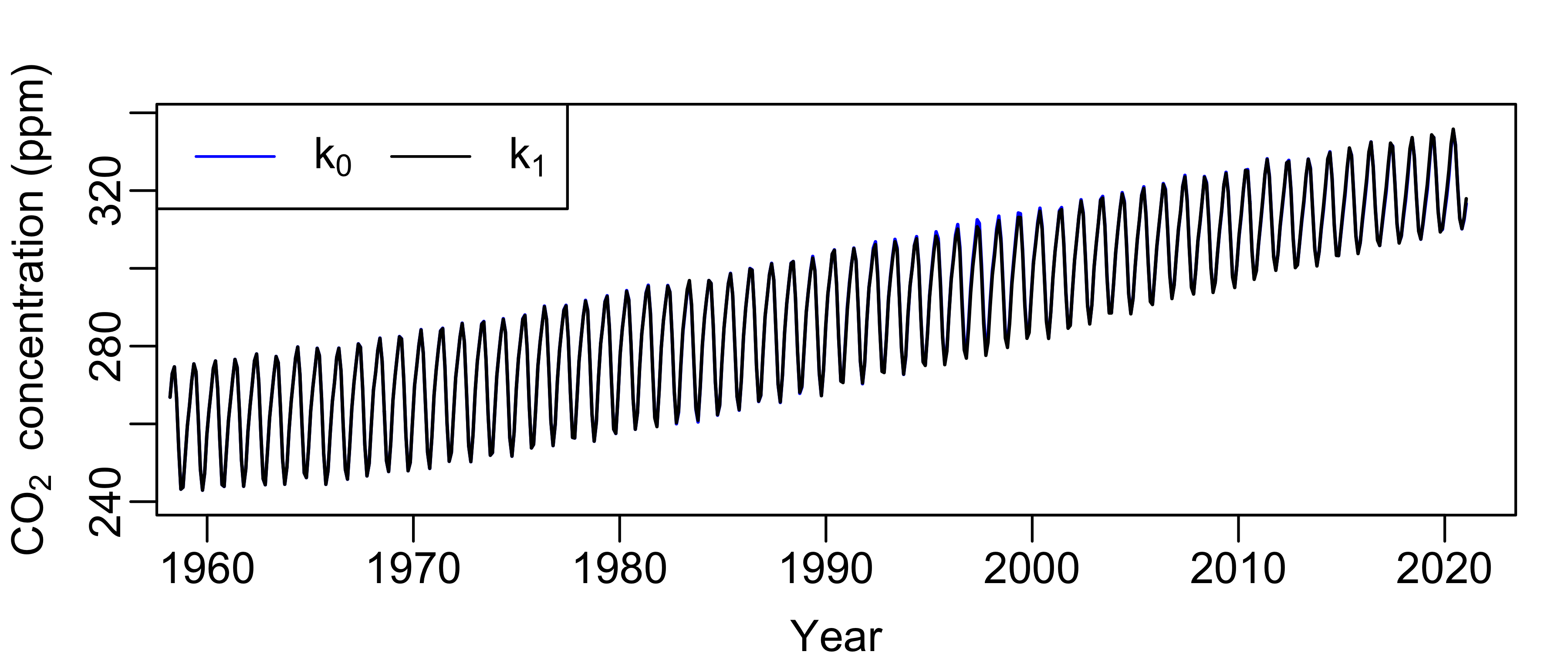
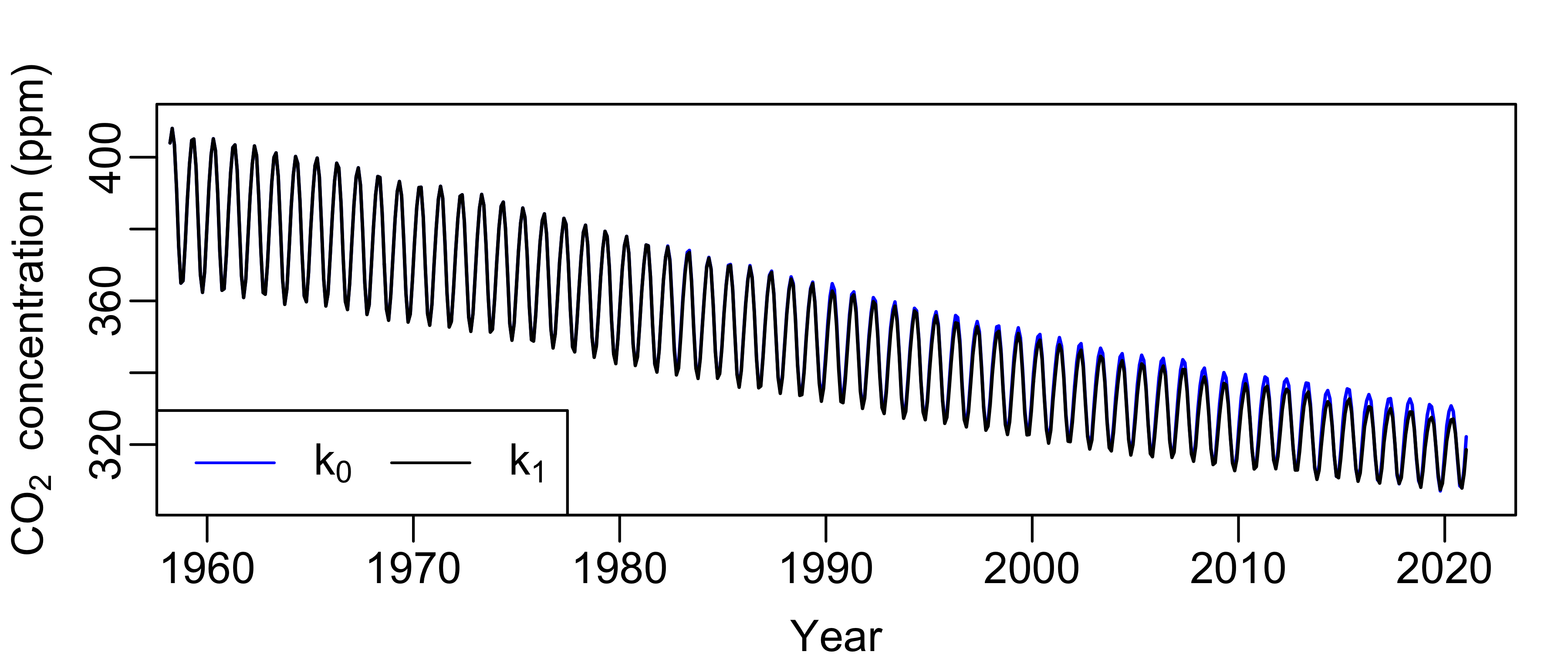
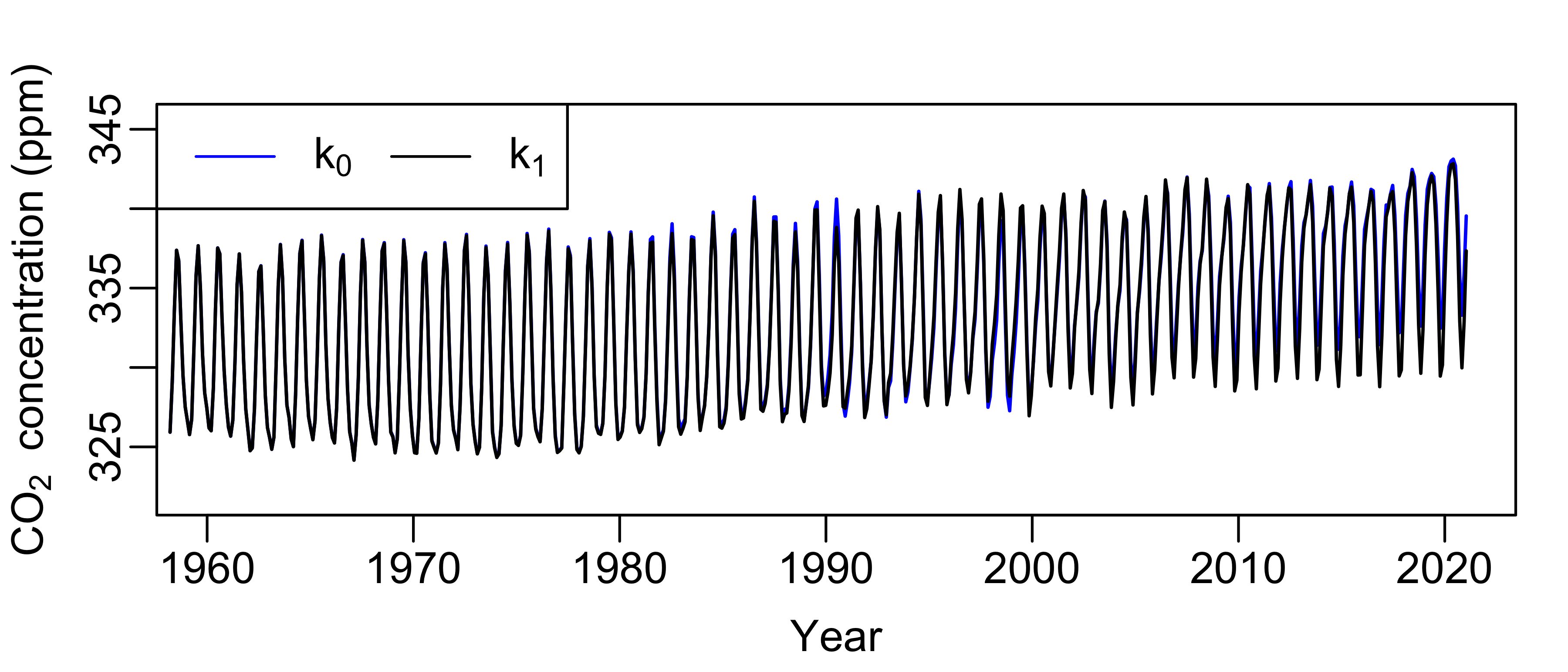
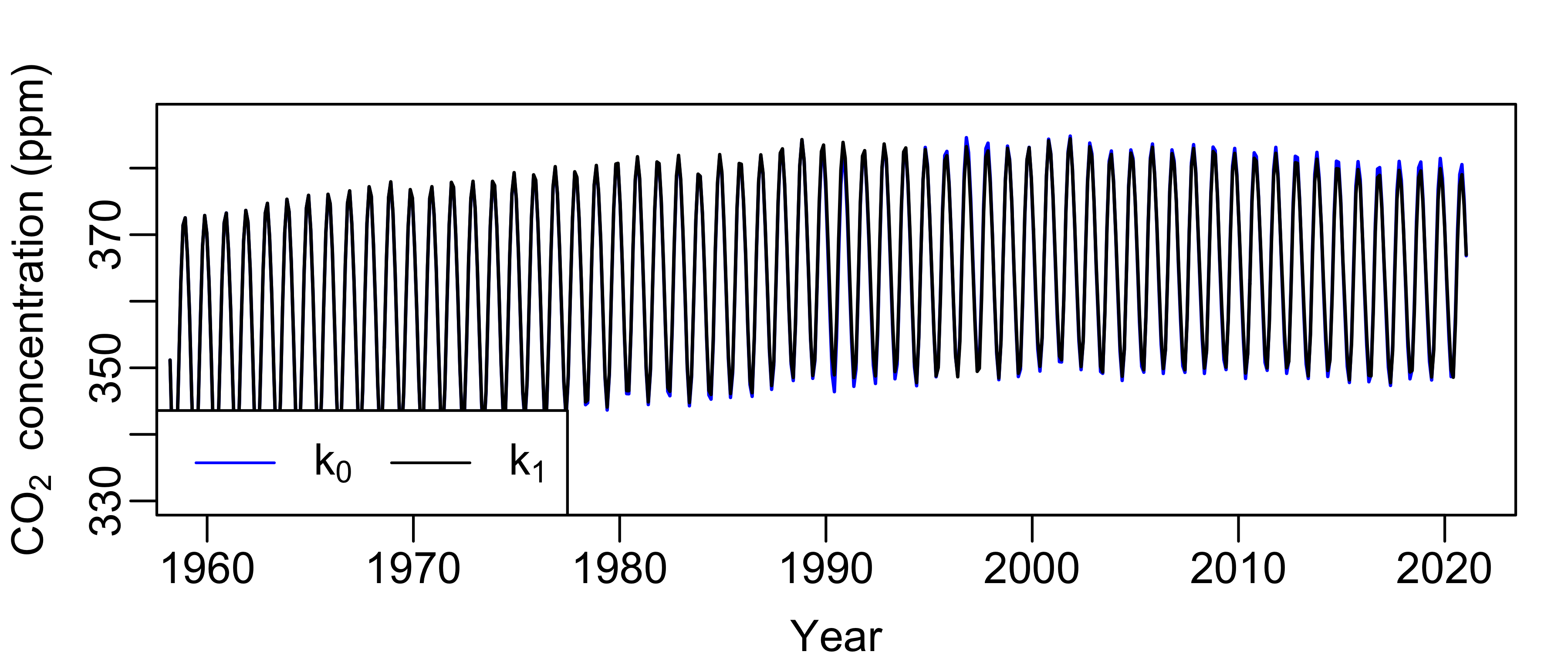
We plot noise matched prior draws for $k_{0}$ and $k_{1}(\varepsilon^{*})$ in Fig. 8. The samples from $k_{1}(\varepsilon^{*})$ appropriately line up with the expected maxima and minima of CO₂ levels (to see this, note that the draws from $k_{1}(\varepsilon^{*})$ are in-phase with those from $k_{0}$, which correctly captures the seasonal maxima and minima). The deviations between the noise-matched samples do not seem significant, so we say that $k_{1}(\varepsilon^{*})$ and $k_{0}$ are qualitatively interchangeable. Further, we find that the distance between $k_{1}(\varepsilon^{*})$ and $k_{0}$ is smaller than what we might expect to arise from sampling uncertainty about $k_{0}$’s hyperparameters (see Fig. 16 in Appendix G). We therefore conclude that the prediction of CO₂ levels under $k_{0}$ is non-robust to the choice of the kernel in the sense of Definition 1.

The Mauna Loa experiments were run on a laptop with a 2.3 GHz 8-Core Intel Core i9, with 64 GB of RAM. The experiment (which optimizes from five random initialization) took about 15 minutes to run, with each seed taking about 3 mins.

Appendix E CO₂ experiments using the automatic statistician

Here we use the kernel learned by the automatic statistician Duvenaud et al., (2013) to model the Mauna-Loa CO₂ data. The automatic statistician kernel is:

$$k_{0}(x_{1},x_{2}) =\left(\theta_{1}^{2}+\theta_{2}^{2}(x_{1}-\theta_{3})(x_{2}-\theta_{3})\right)\times\theta_{4}^{2}\exp\left(-\frac{(x_{1}-x_{2})^{2}}{2\theta_{5}^{2}}\right)$$ (12)

$$+\theta_{6}^{2}\exp\left(-\frac{2\sin^{2}(\pi(x_{1}-x_{2})/\theta_{7})}{\theta_{8}^{2}}\right)\times\theta_{9}^{2}\exp\left(-\frac{(x_{1}-x_{2})^{2}}{2\theta_{10}^{2}}\right)$$ (13)

$$+\theta_{11}^{2}\left(1+\frac{(x_{1}-x_{2})^{2}}{2\theta_{12}^{2}\theta_{13}}\right)^{-\theta_{14}}\times\theta_{15}^{2}\exp\left(-\frac{(x_{1}-x_{2})^{2})}{2\theta_{16}^{2}}\right).$$ (14)

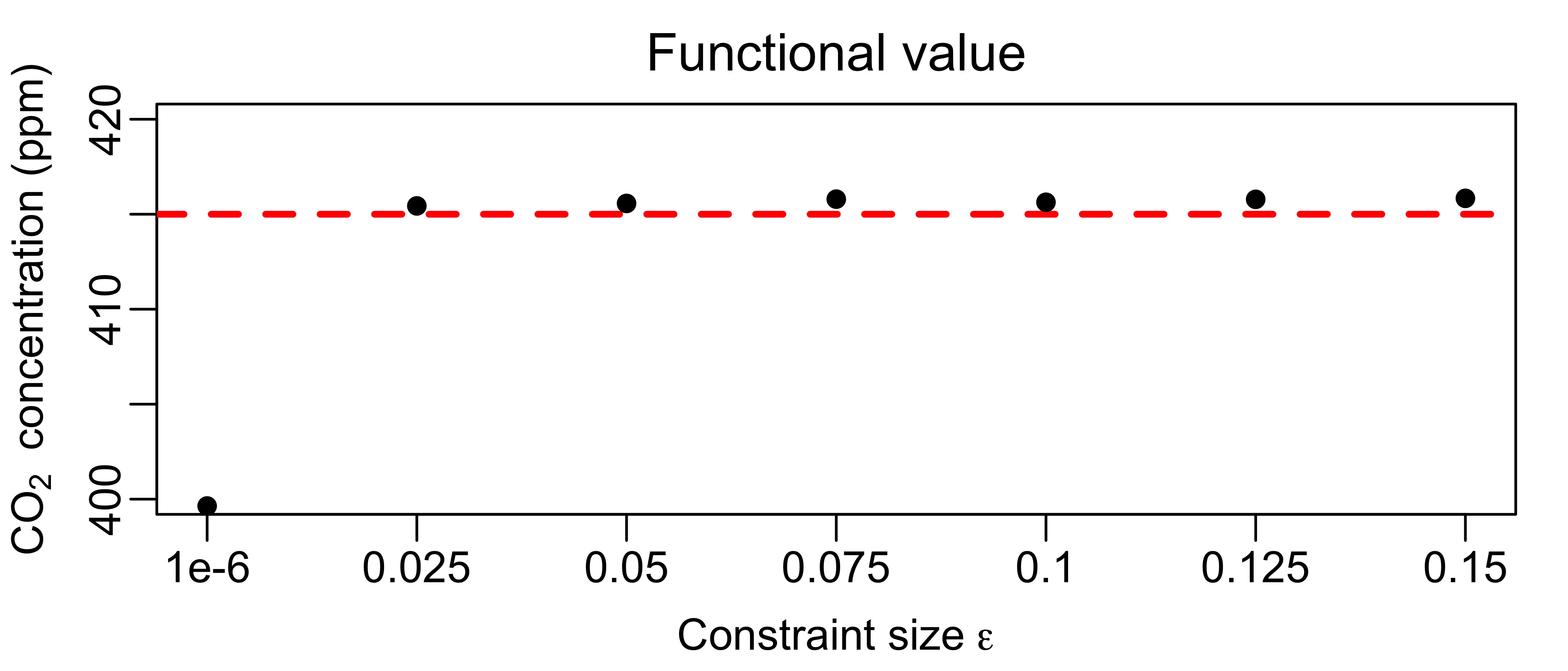
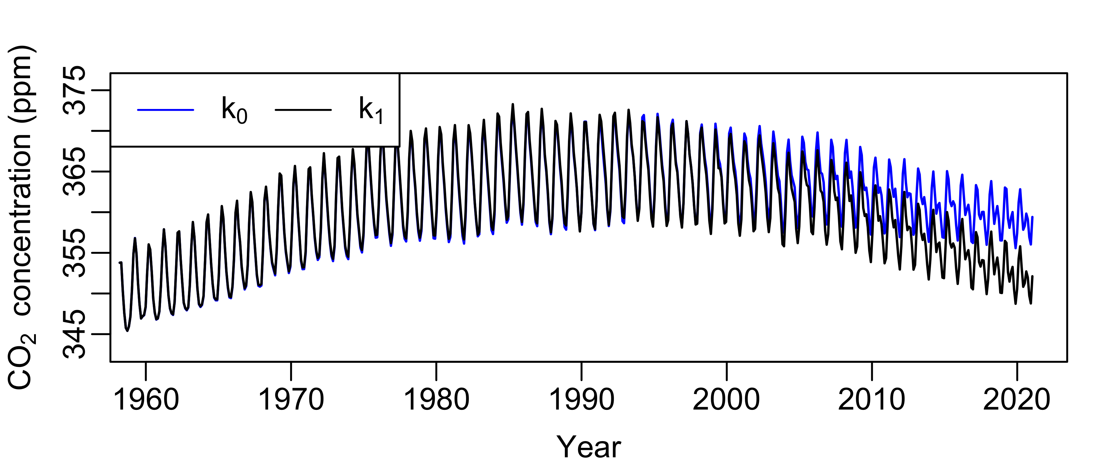
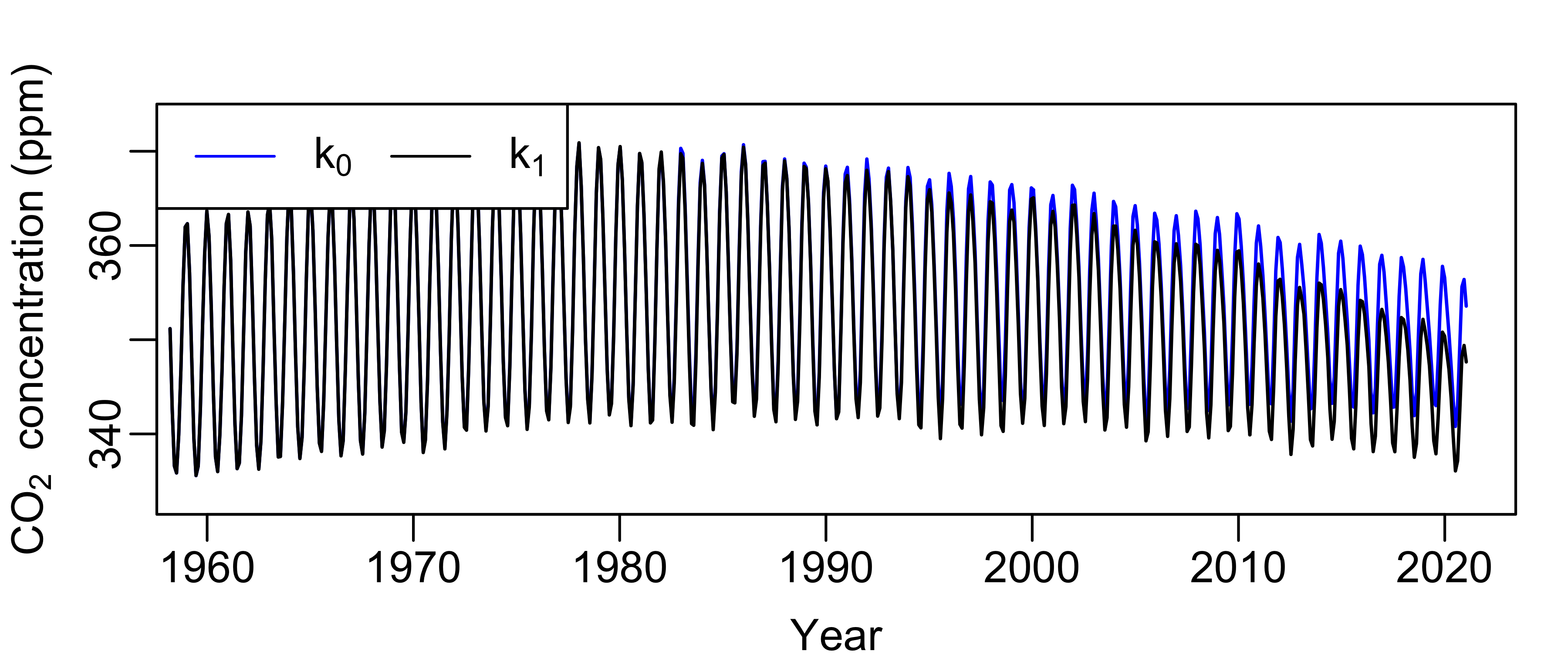
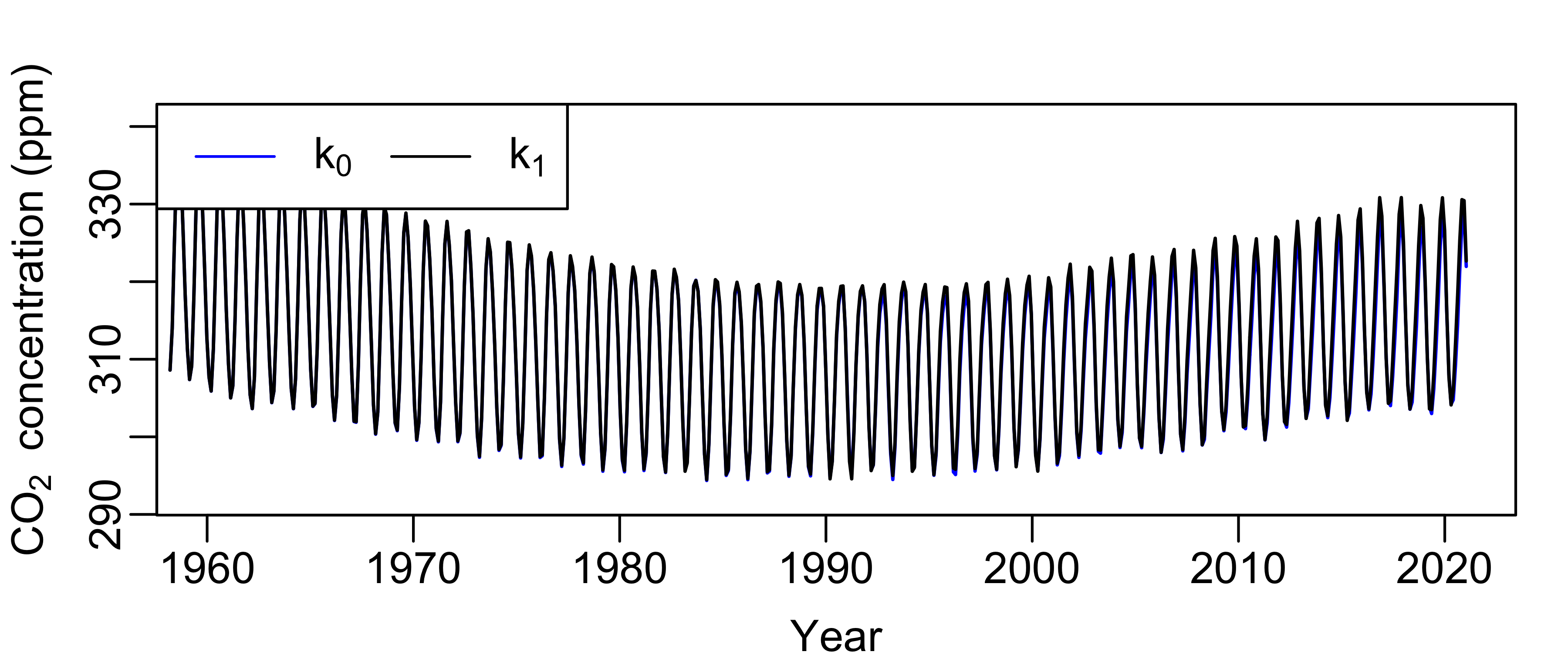
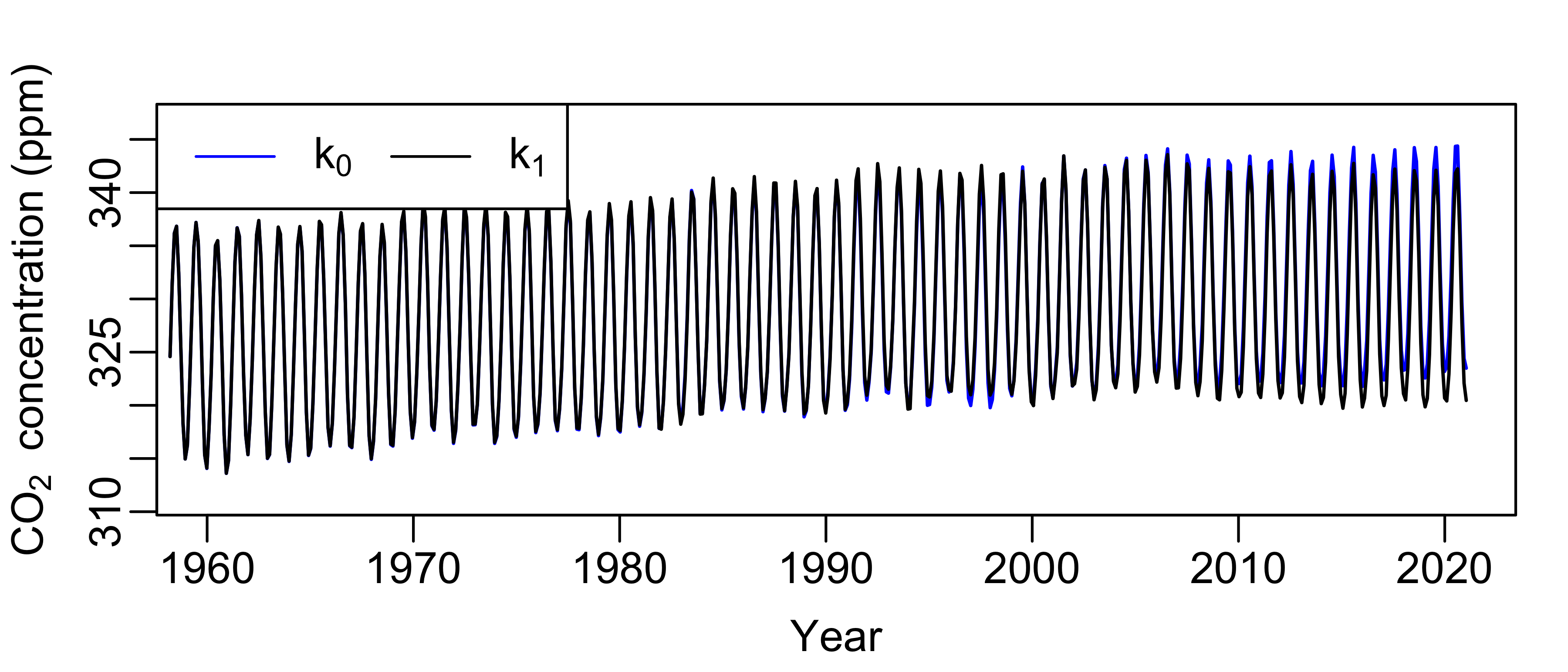
We learned the hyper-parameters of the kernel by maximizing the marginal likelihood on data up till $2003$, mimicking the process used for learning the parameters of the hand designed kernel described in Appendix D. Fig. 9 presents analogous results to those presented in Fig. 5 for the hand designed kernel.

Figure 9: Sensitivity of the Mauna Loa analysis in Appendix E. (Top-left): Predictions made with the automatic statistician kernel $k_{0}$ (black) and a qualitatively interchangeable kernel $k_{1}$ (red). (Top-right): $F^{\star}$, the mean CO₂ level in June 2020, as a function of $\varepsilon$. (Bottom): Noise-matched draws from a $\mathcal{GP}(0,k_{0})$ (left) and $\mathcal{GP}(0,k_{1}(\varepsilon^{*}))$ (right) prior. See Fig. 10 for a closer inspection of each prior draw.

Figure 10: Sensitivity analysis of Mauna Loa. Each plot shows noise matched samples from a zero mean Gaussian process with original and perturbed kernel functions. These plots provide a zoomed in view of the prior samples shown in Fig. 9. We note that draws from $k_{1}(\varepsilon^{*})$ are in-phase with those of $k_{0}$ (i.e. $k_{1}(\varepsilon^{*})$ captures the seasonal maxima and minima of CO₂ just as well as $k_{0}$ does). Overall, there is high agreement between functions sampled from the two GPs.

Appendix F More details on MNIST experiments

Figure 11: Additional MNIST experiments. Here we visualize the training and test set performances along the hyperparamter grid used for assessing qualitative interchangeability. The train and test accuracies exhibit high performance and low variability across the grid.

Figure 12: Example test images from Section 5. $\bm{x}^{\star}$ (upper) and their warps $g(\bm{x}^{\star})$ (lower) and predicted class labels (above and below).

We use the publicly available neural-tangents (Novak et al.,, 2020) package for constructing the kernels in our MNIST experiments. We follow the experimental setup of Lee et al., (2018) where the authors use a Gaussian process with a kernel corresponding to a $20$ layer, infinitely wide, fully connected, deep neural network with ReLU non-linearities. They place zero mean Gaussian priors over the weights, $\mathcal{N}(0,\sigma^{2}_{w})$, and biases, $\mathcal{N}(0,\sigma^{2}_{b})$, and set the hyper-parameters $\sigma^{2}_{w}=1.45$ and $\sigma^{2}_{b}=0.28$ via a grid search over parameters to maximize held-out predictive performance. Lee et al., (2018) use a GP with $C=10$ outputs (classes). They pre-process one-hot encoded output vectors to have zero mean, i.e. $y_{ic}=0.9$ if $c$ is the correct class for the $i$th training point, and $y_{ic}=-0.1$ for all incorrect classes; input images are flattened and an overall mean is subtracted from every image. Test prediction is made by selecting a class corresponding to the GP output with mean closest to $0.9$. The resulting GP trained on one thousand images from the MNIST training set and evaluated on the MNIST test set achieves an accuracy of $92.79\%$.

In our experiments we assess the robustness of their kernel. The $28\times 28$ MNIST images require a warping function $g:\mathbb{R}^{784}\rightarrow\mathbb{R}^{784}$. We use a fully connected multi-layer perceptron with one $784$ unit hidden layer, $784$ input, and $784$ output units with ReLU non-linearities to parametrize $g$. Let $c_{0}$ be the prediction under the original kernel at a target test image $\bm{x}^{\star}$. We define $c_{1}:=|c_{0}-1|$ and create a “fake” output $y^{*}$ with $y^{*}_{c_{1}}=0.9$ and $y^{*}_{c}=-0.1$ for $c\neq c_{1}$. We find parameters of $g$ by minimizing the objective in Algorithm 3 plugging in

$$\ell(k;F^{\star},L)=-\frac{1}{C}\sum_{c=1}^{10}\log p(y^{*}_{c}|X,\bm{x}^{\star},Y),$$ (15)

i.e. the negative log-likelihood of the “fake” output at a particular test image $\bm{x}^{\star}$ under the perturbed kernel; $X$ and $Y$ are the train inputs and outputs. As we discussed in the main text, directly optimizing the posterior quantity of interest $F^{\star}=|\mu_{c_{0}}(\bm{x}^{\star})-0.9|-|\mu_{c_{1}}(\bm{x}^{\star})-0.9|$ produces unrealistic outputs, e.g. $\mu_{c_{0}}(\bm{x}^{\star})\ll-0.1$. Such predictions would look obviously suspicious to a user, so we would say that our supposed malicious actor has not achieved their goal in this case. Instead, we optimize the surrogate loss in Eq. 15. With this surrogate loss we are able to find kernel perturbations yielding benign-looking outputs and achieving the goal of the malicious actor to change the prediction at $\bm{x}^{\star}$ to $c_{1}$, i.e. $\mu_{c_{1}}(\bm{x}^{\star})\approx 0.9$ and $\mu_{c}(\bm{x}^{\star})\approx-0.1$ for all $c\neq c_{1}$. In this case, we feel that a user would not be able to identify these predictions as obviously wrong, and so we say that the malicious actor has achieved their goal of changing the predictions of $k_{0}$ without detection.

Hyperparameter sensitivity. To quantify variability in the Gram matrices arising from hyperparameter uncertainty, we vary $\sigma^{2}_{w}$ over $30$ uniformly spaced points between $1.4$ and $1.5$, and $\sigma^{2}_{b}$ over $30$ uniformly spaced points between $0.23$ and $0.33$. This defines a grid that is ten times smaller than the grid Lee et al., (2018) optimize their hyperparameters over when searching for $\hat{\theta}$. Thus we have no reason to pick $\hat{\theta}$ as the true optimum over any of our grid points; that is, our grid points provide a natural (conservative) notion of uncertainty in $\hat{\theta}$. Fig. 11 shows that over the $900$ possible hyperparameter combinations the train and test accuracies remain high and exhibit low variability.

The experiment took approximately 55 minutes to run for a single test image. We ran the computations for the 1000 test images in parallel on a compute cluster with Intel Xeon E5-2667 v2, 3.30GHz cores, requesting one core each time.

Appendix G Additional Gram matrix comparisons

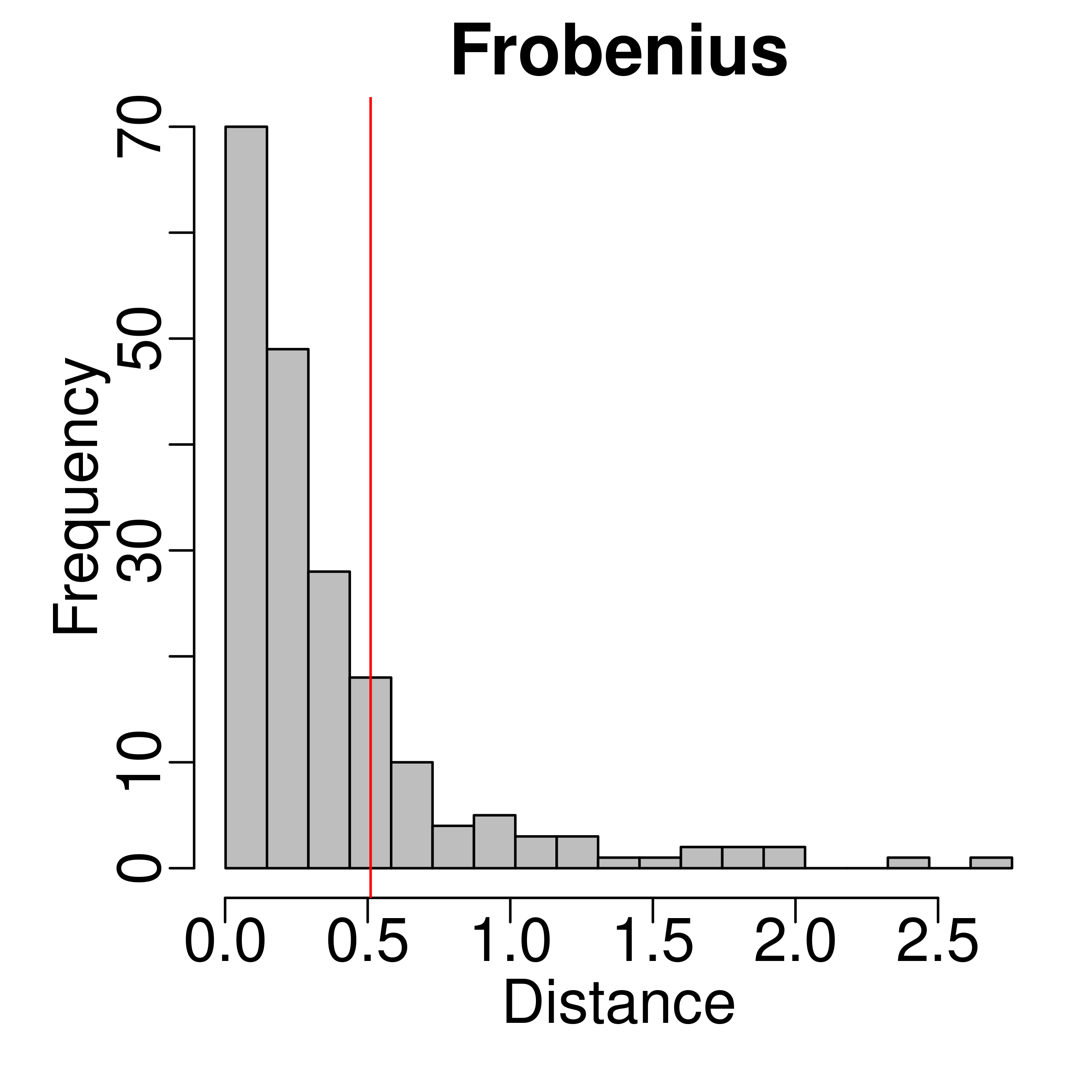
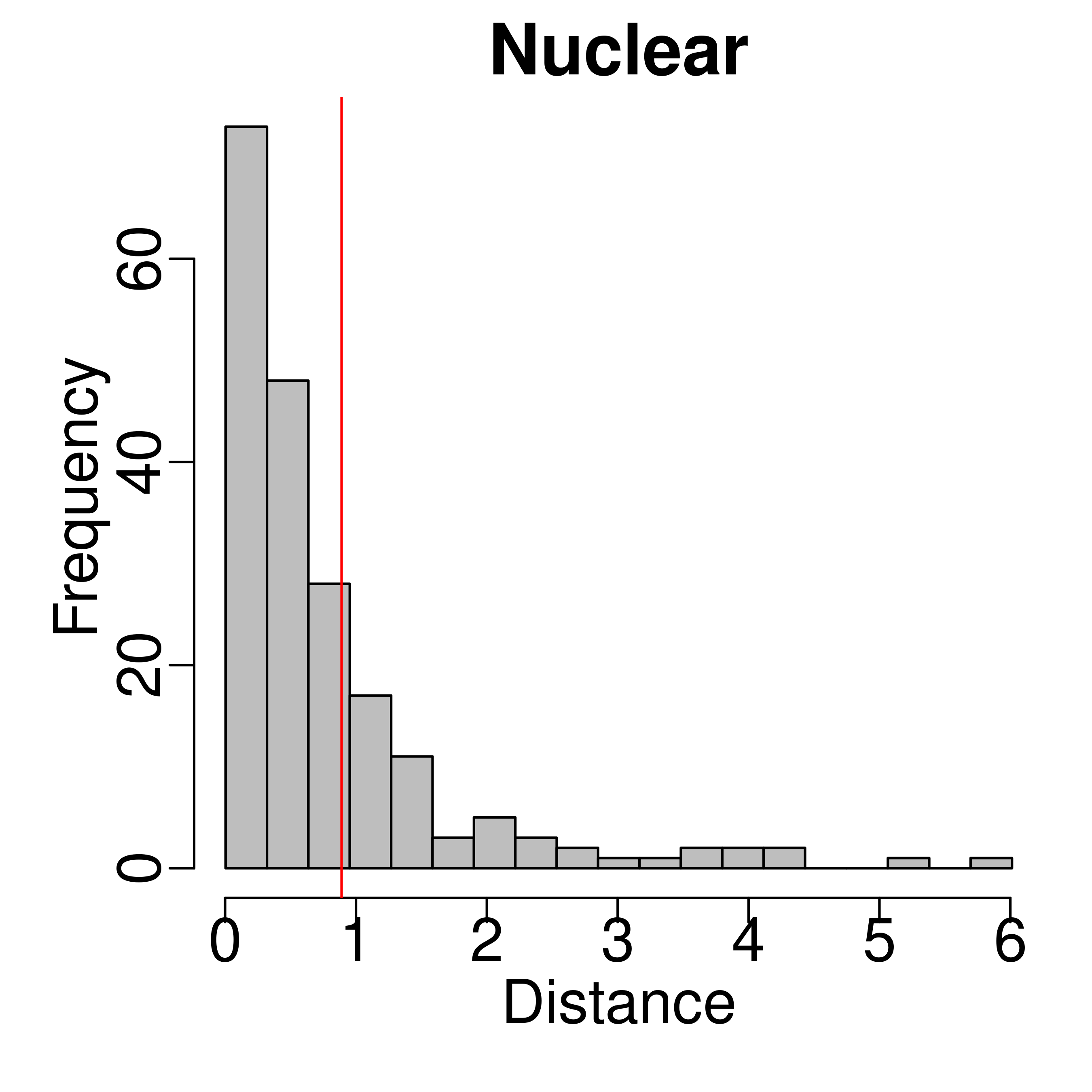
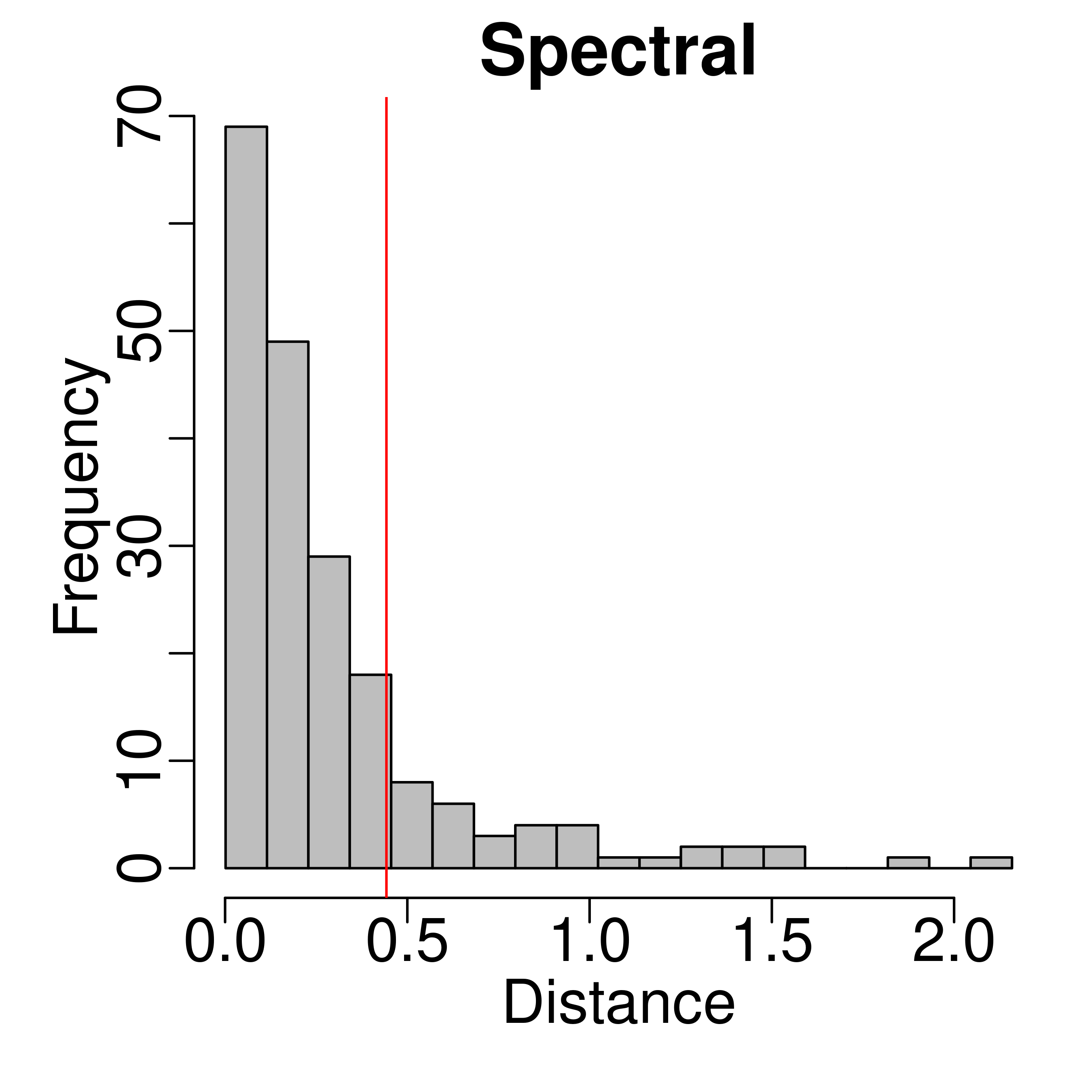
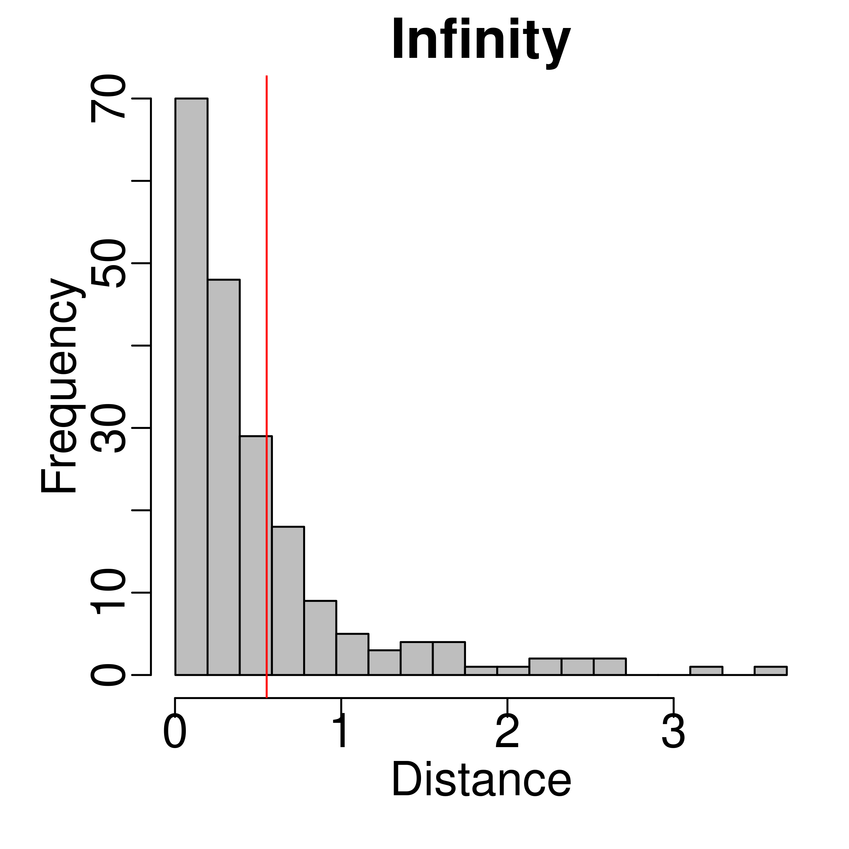
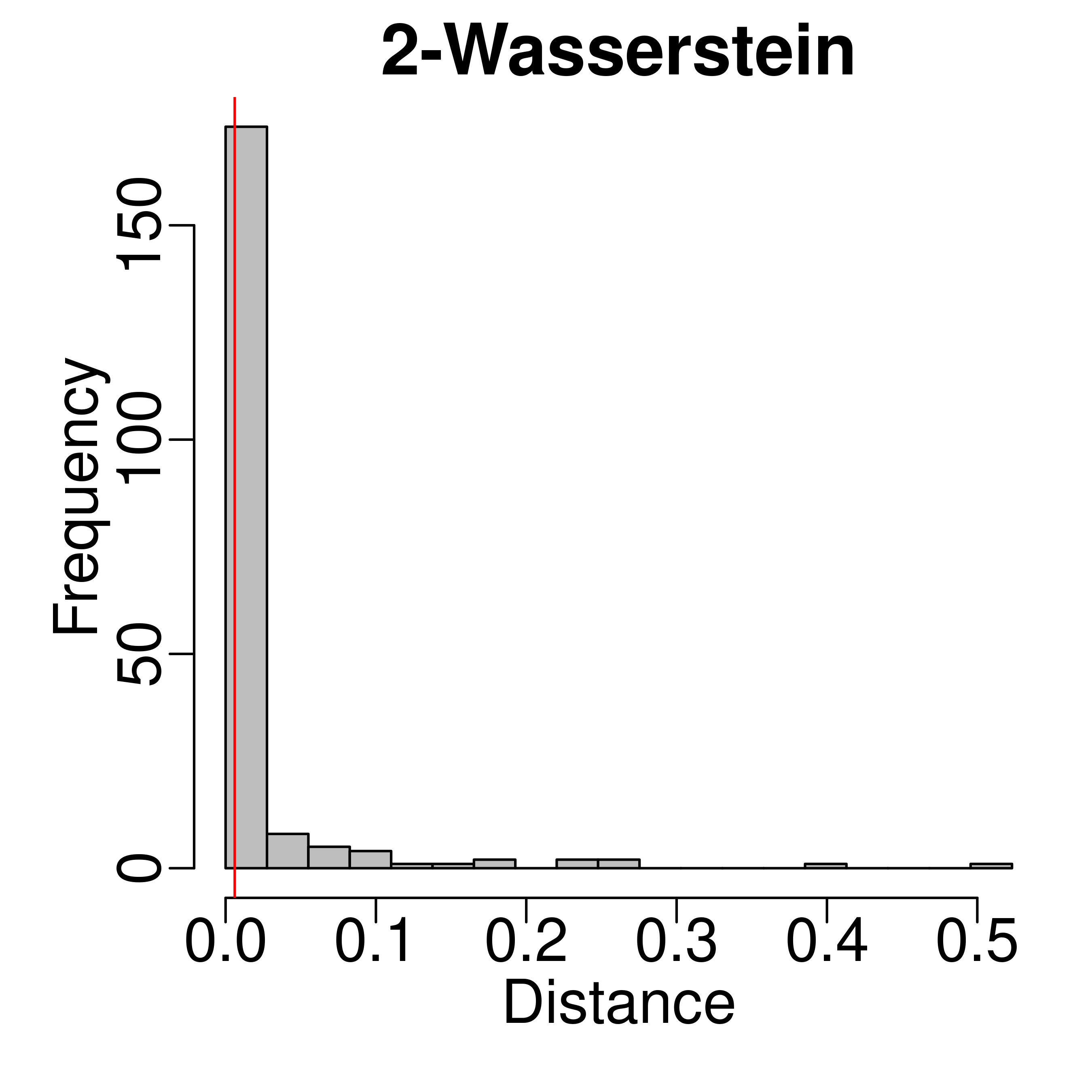
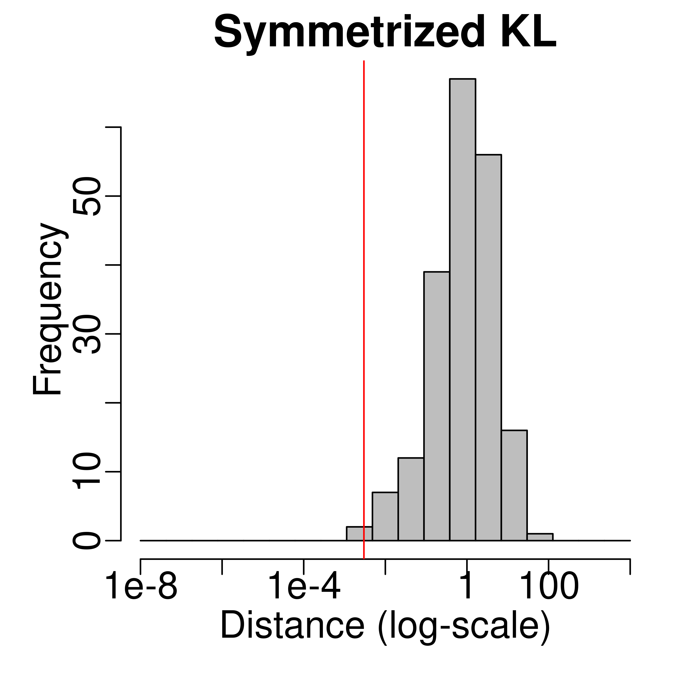
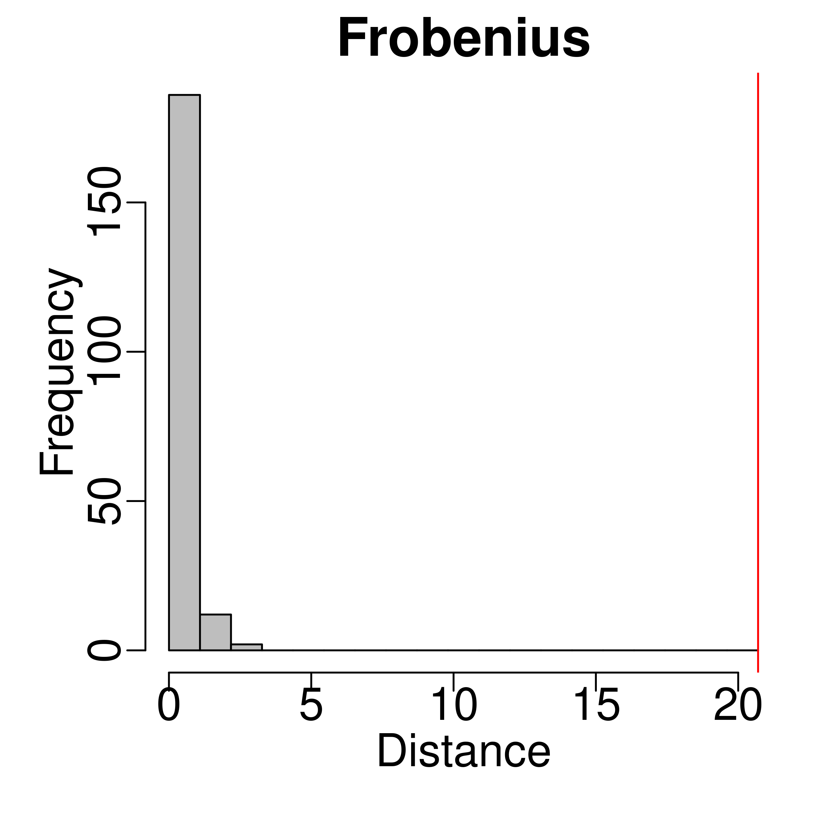
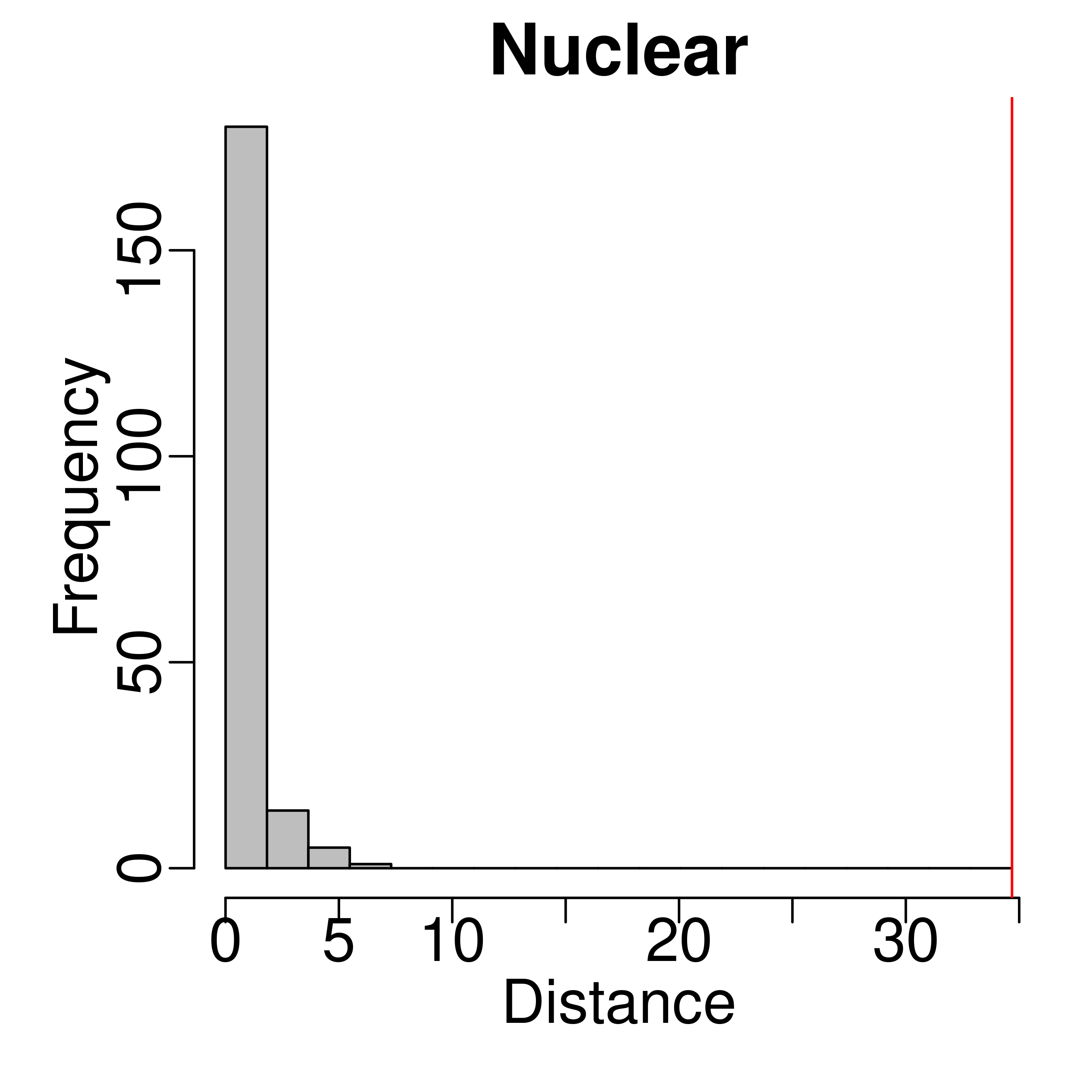
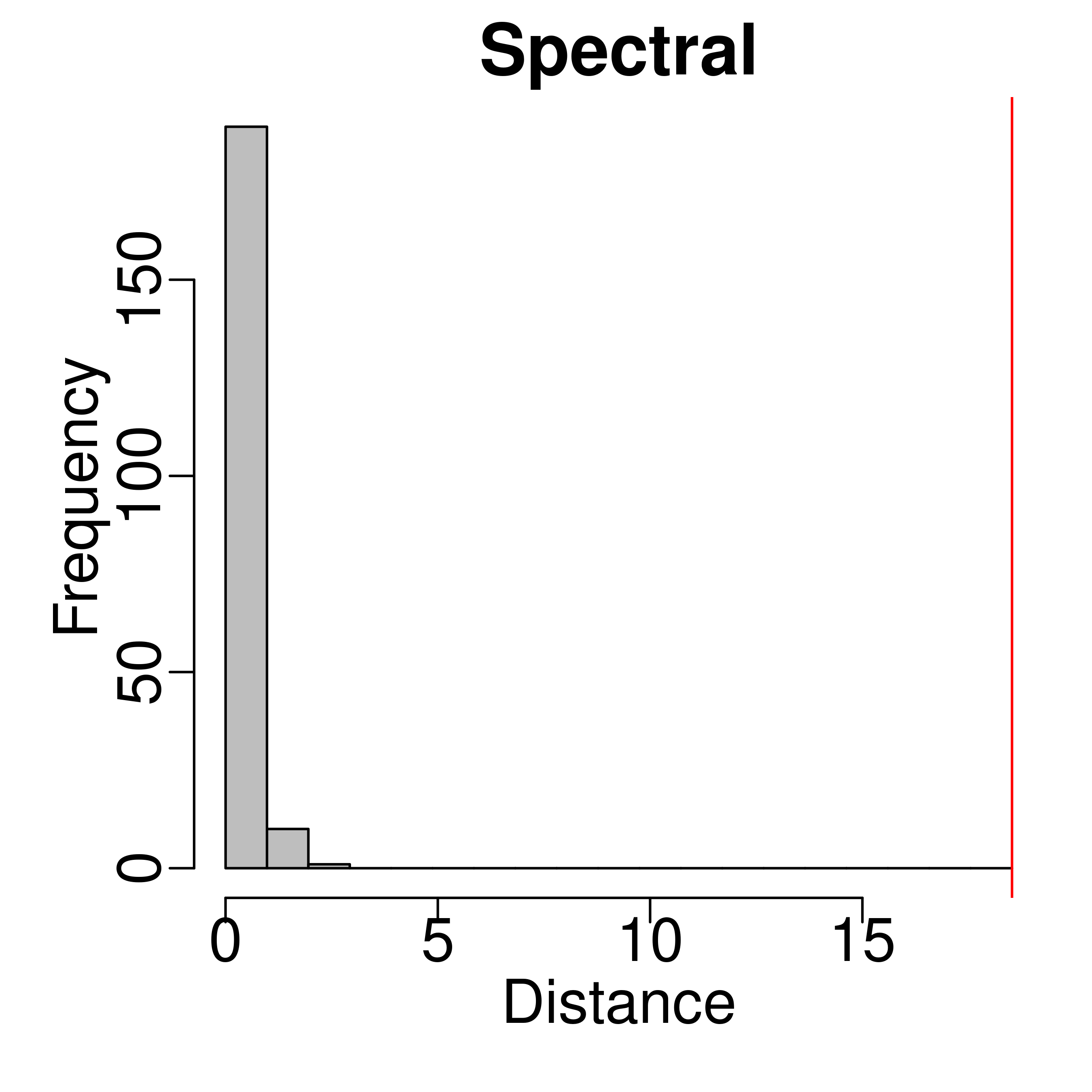
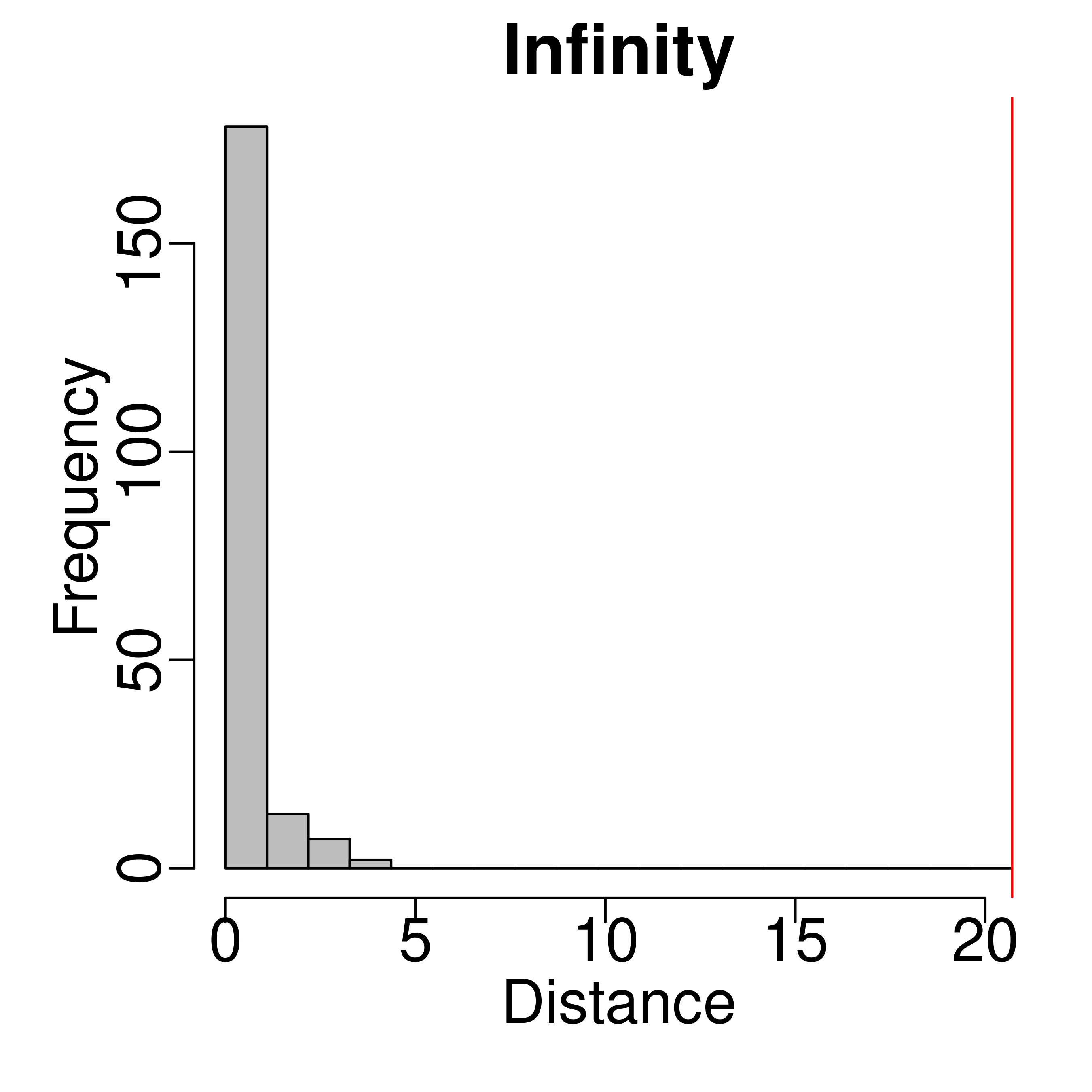
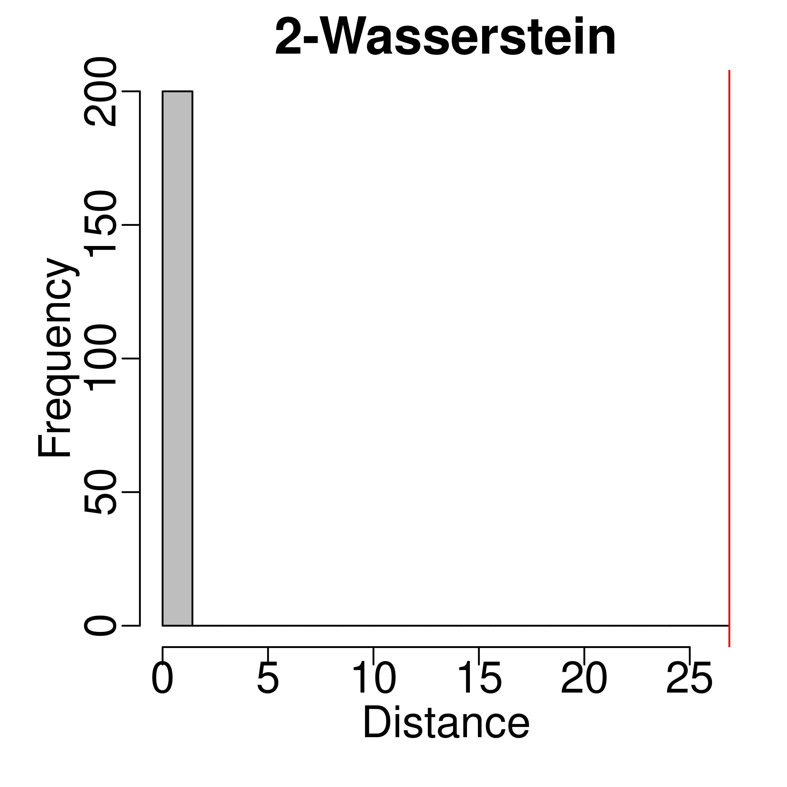
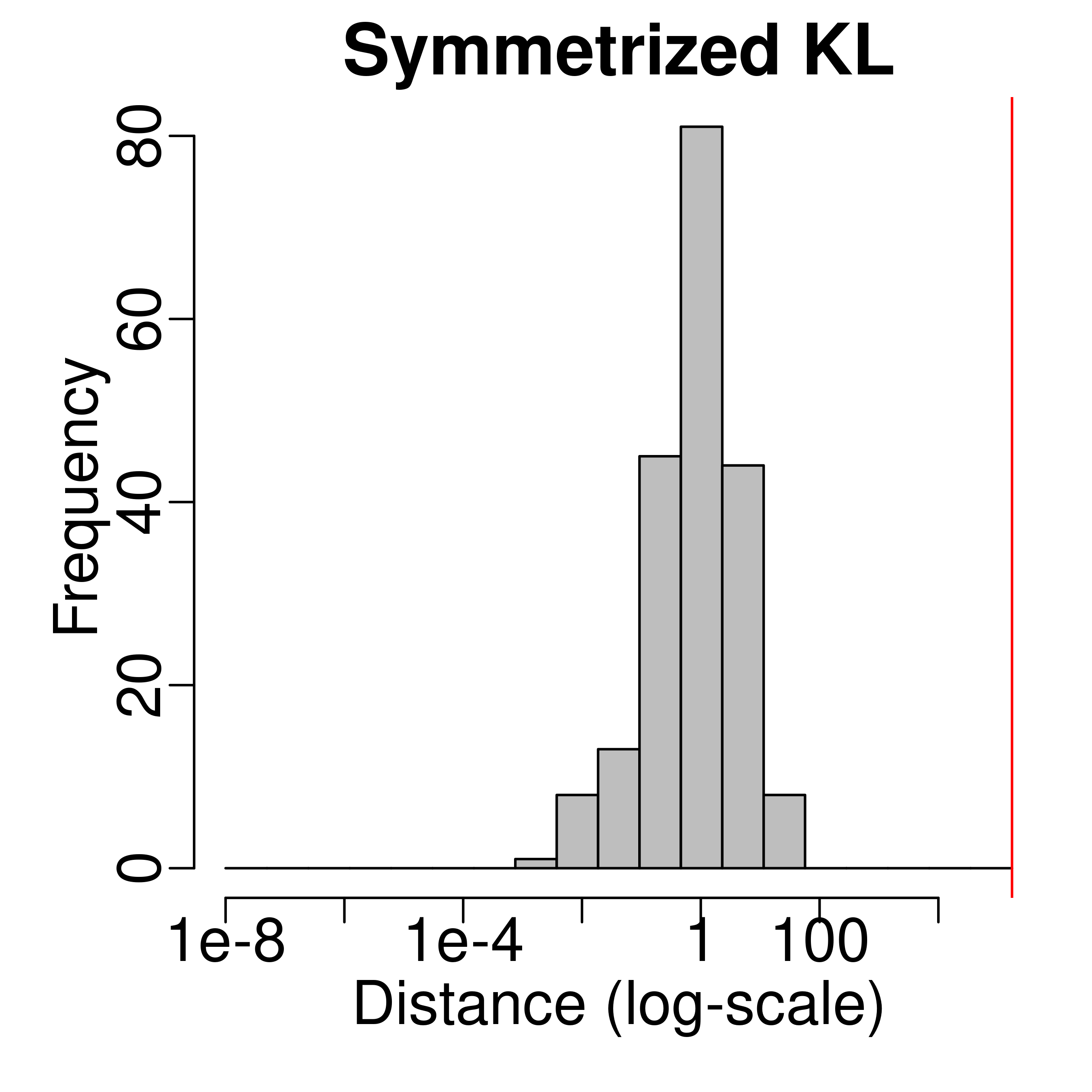
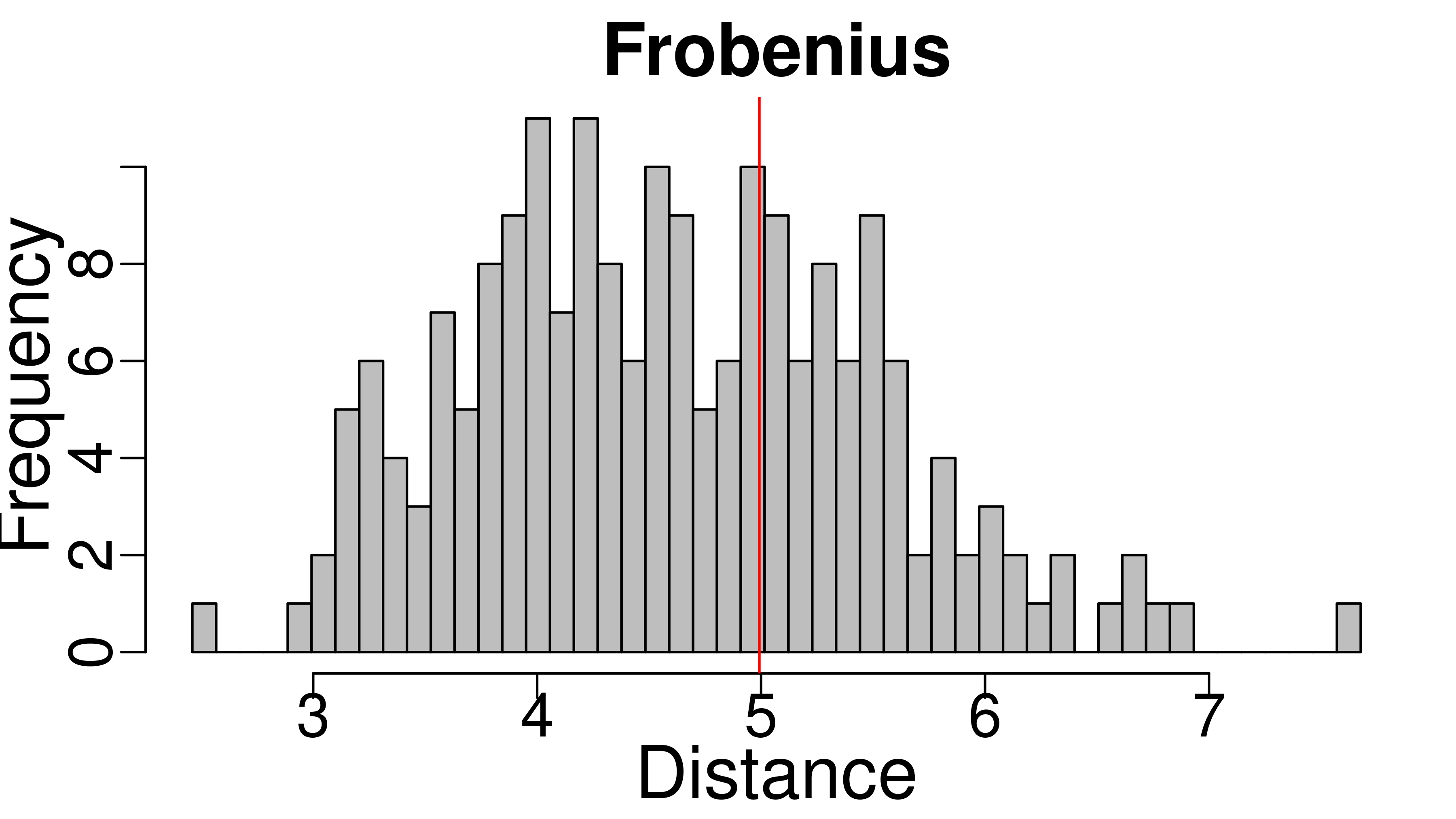
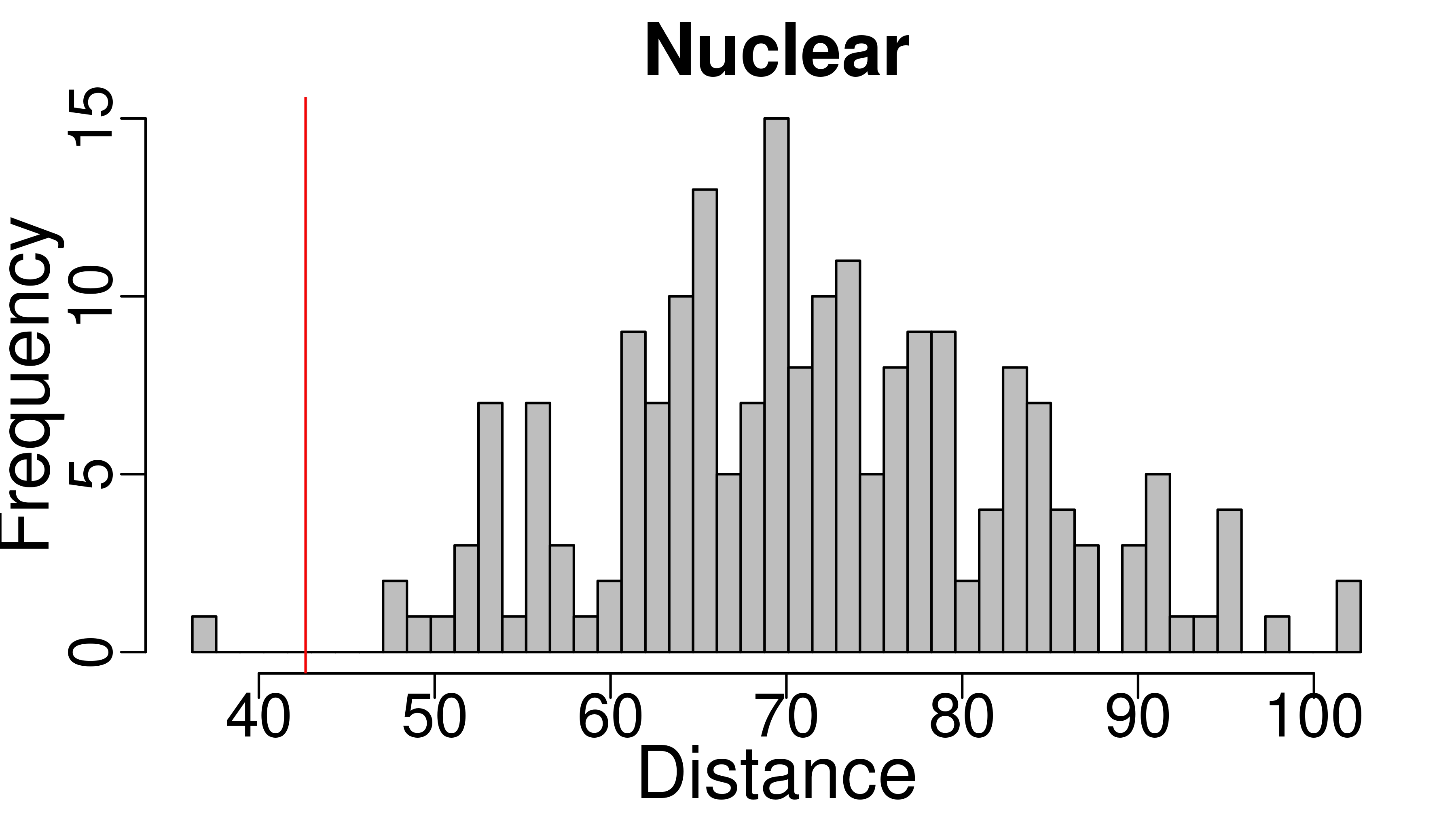
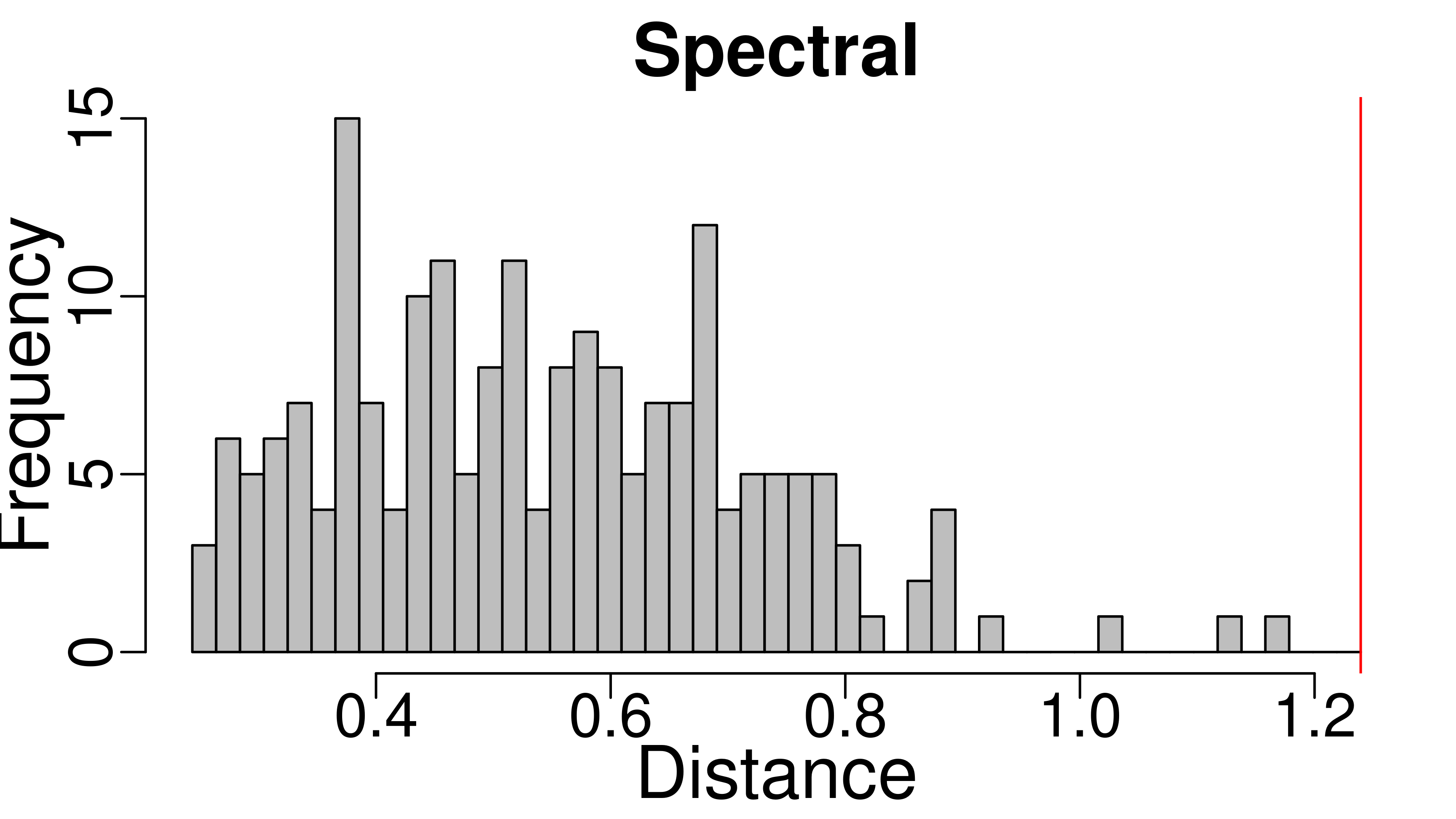
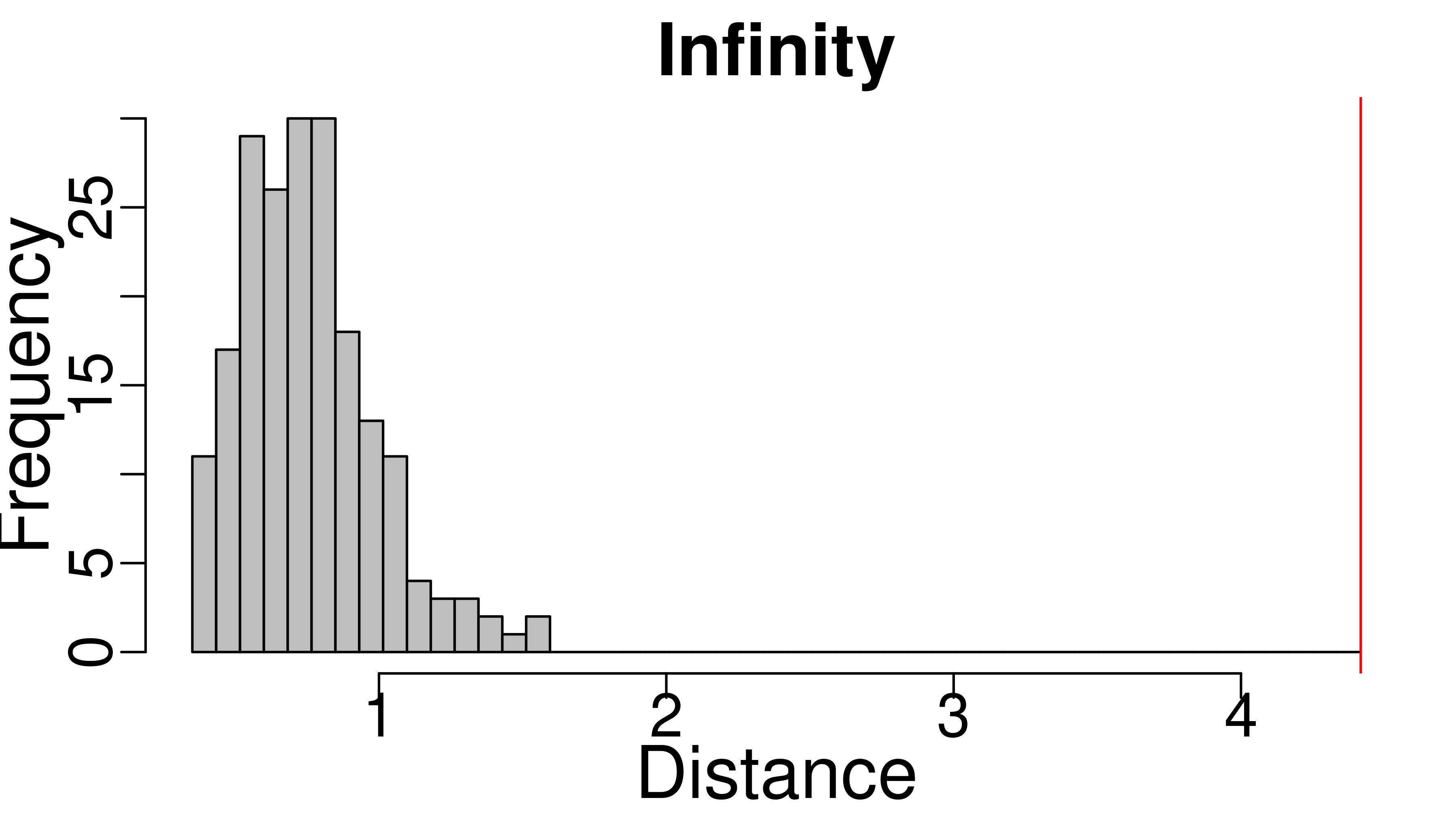
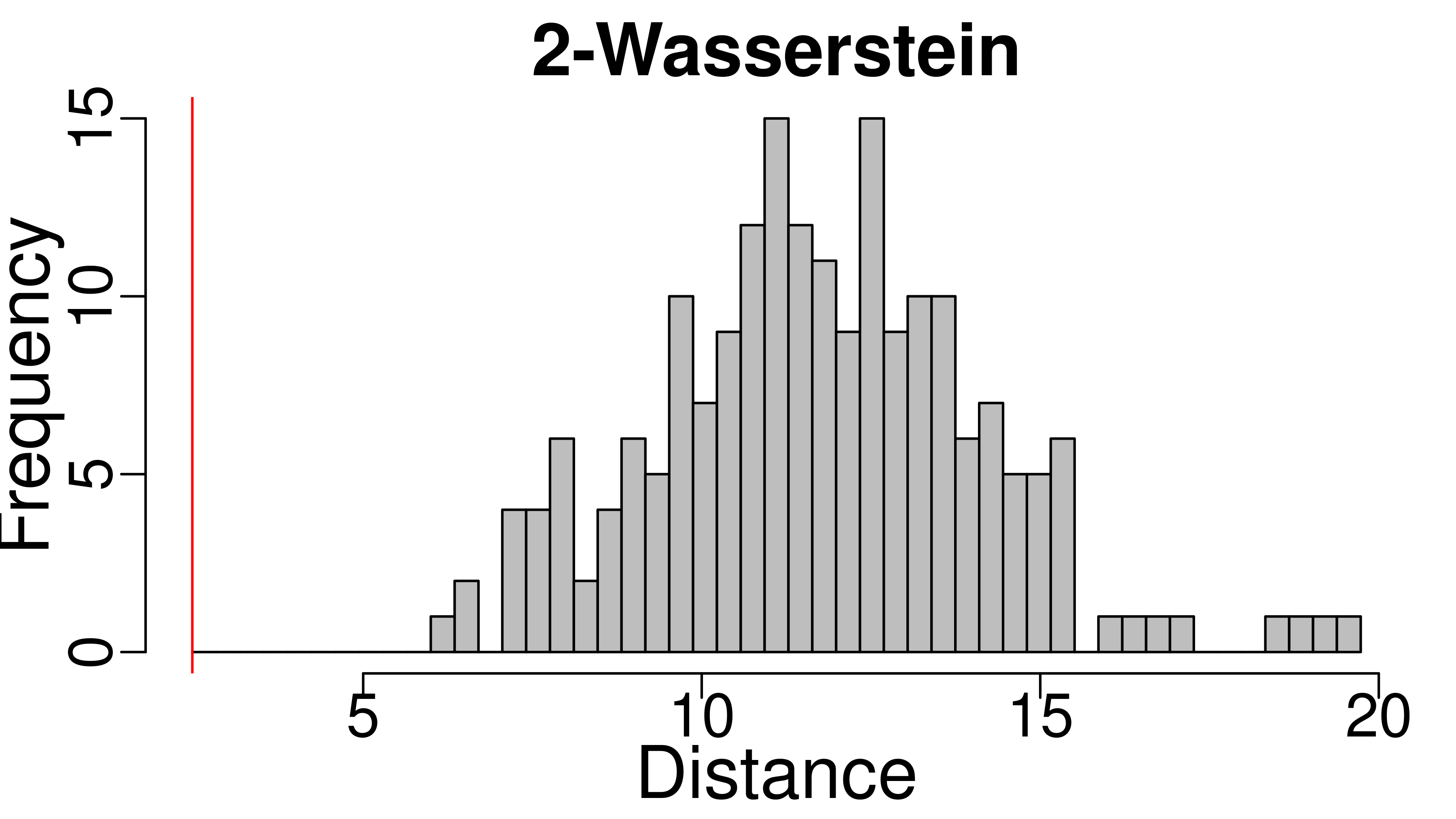
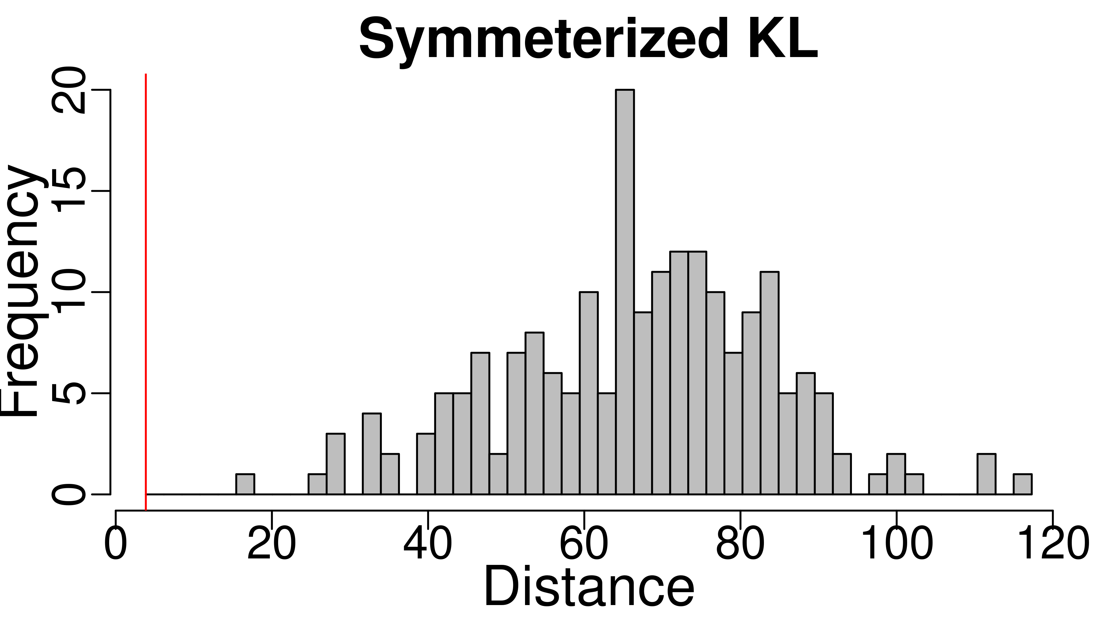
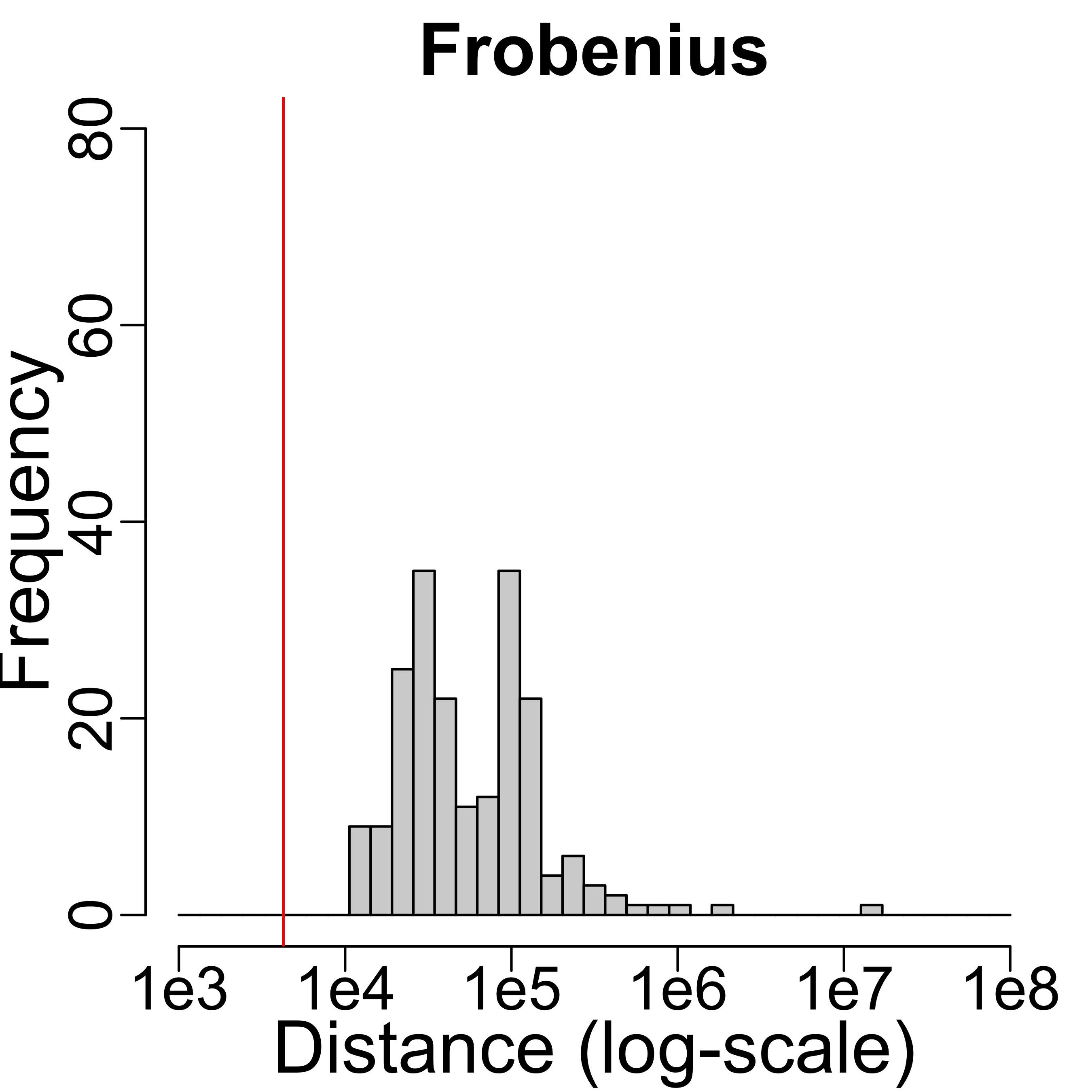
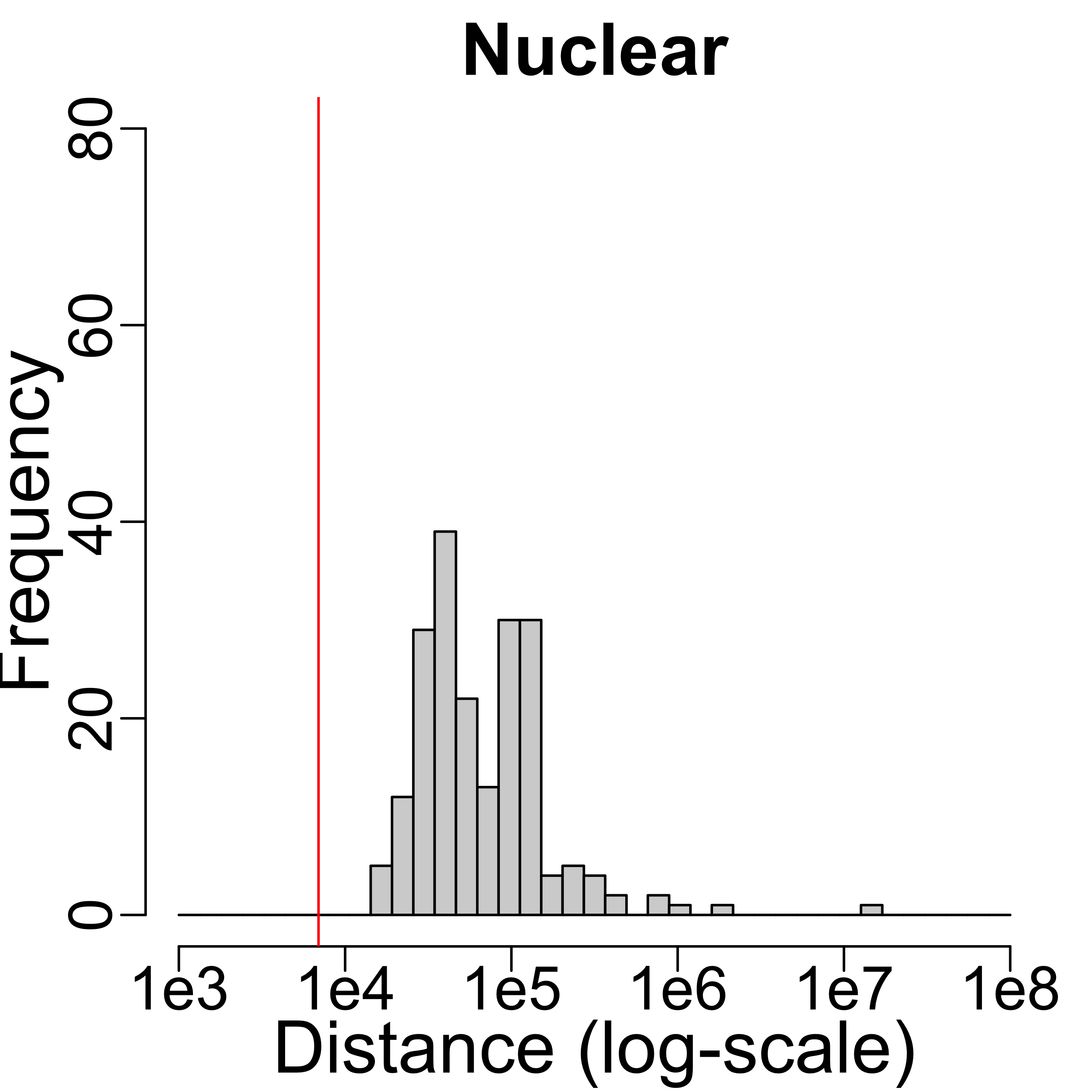
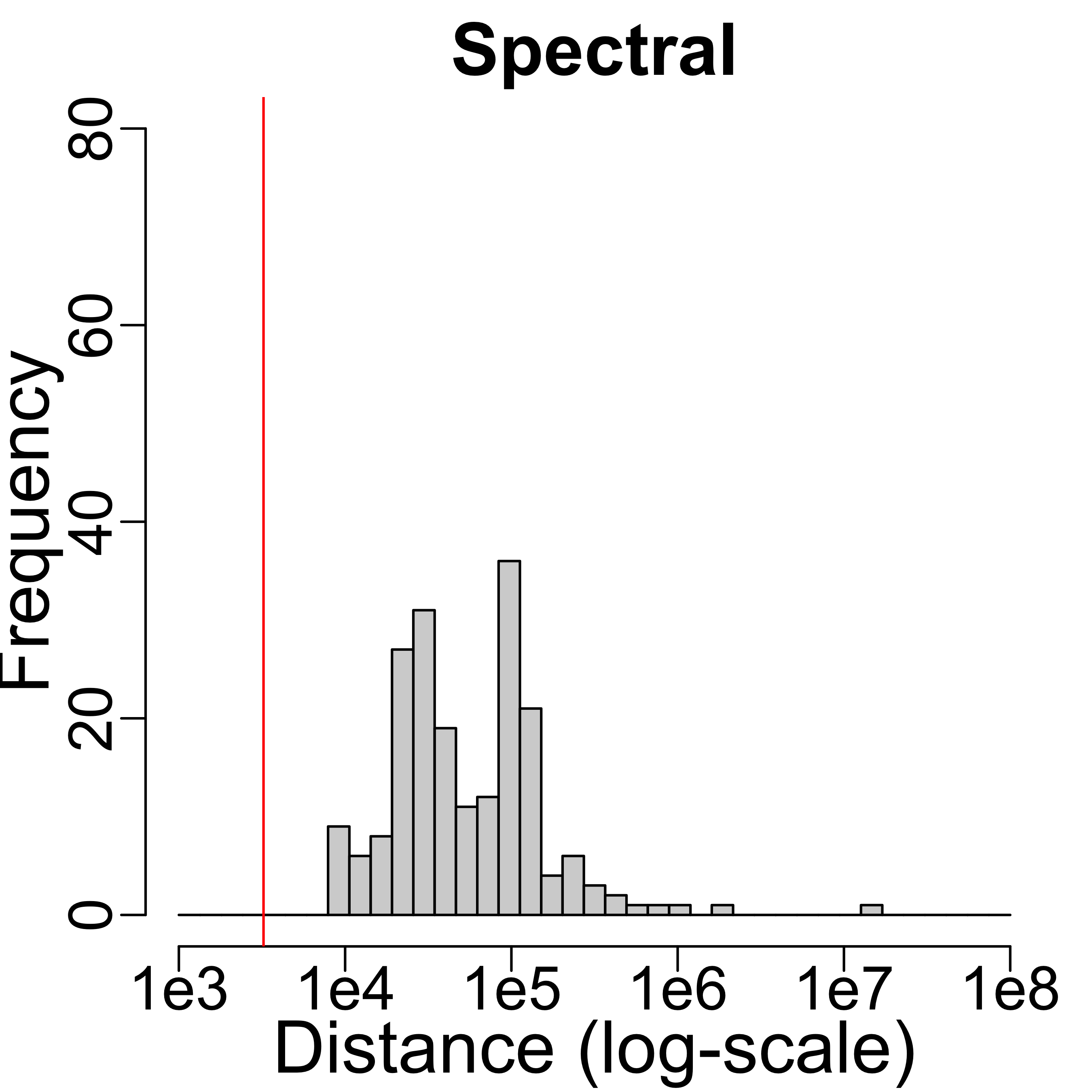
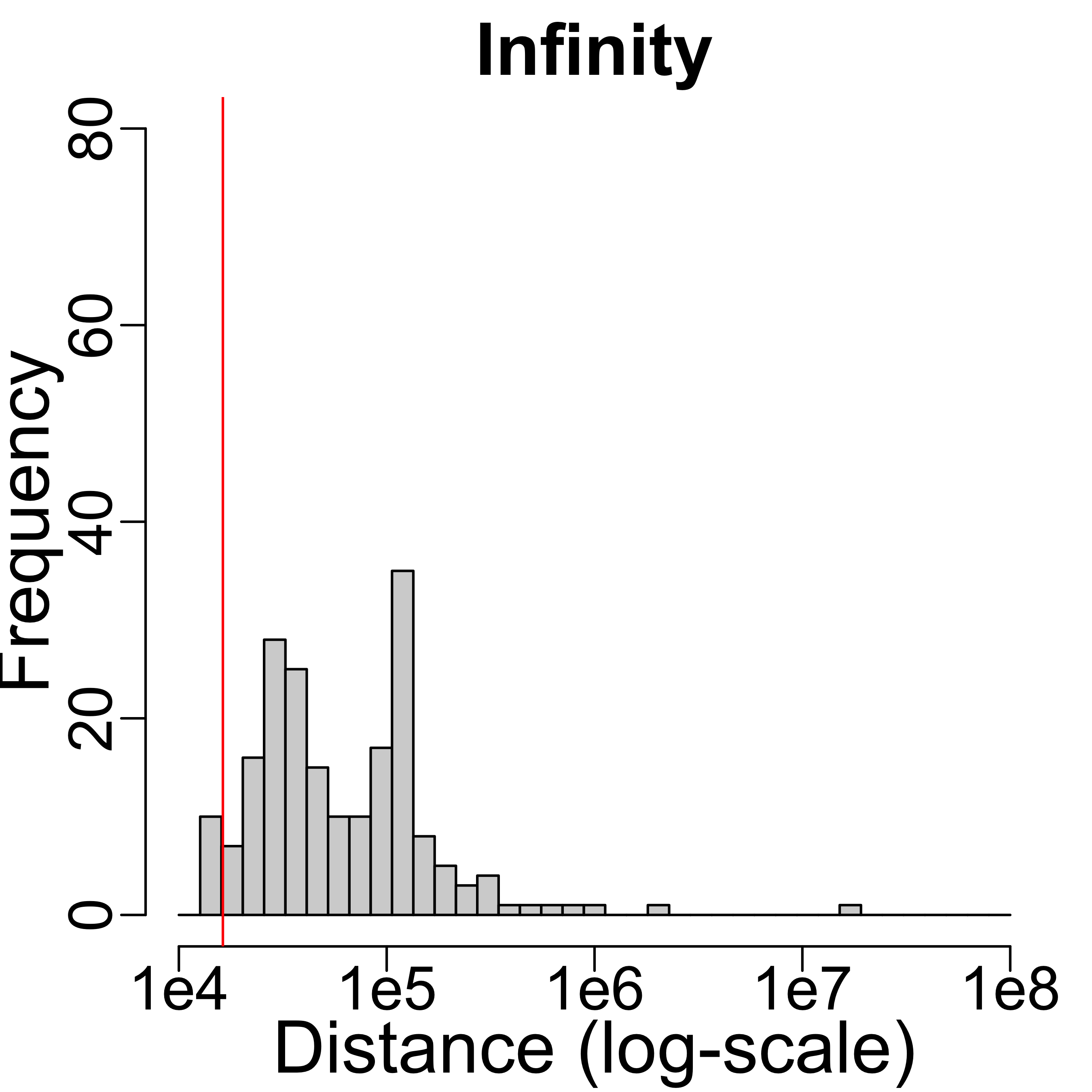
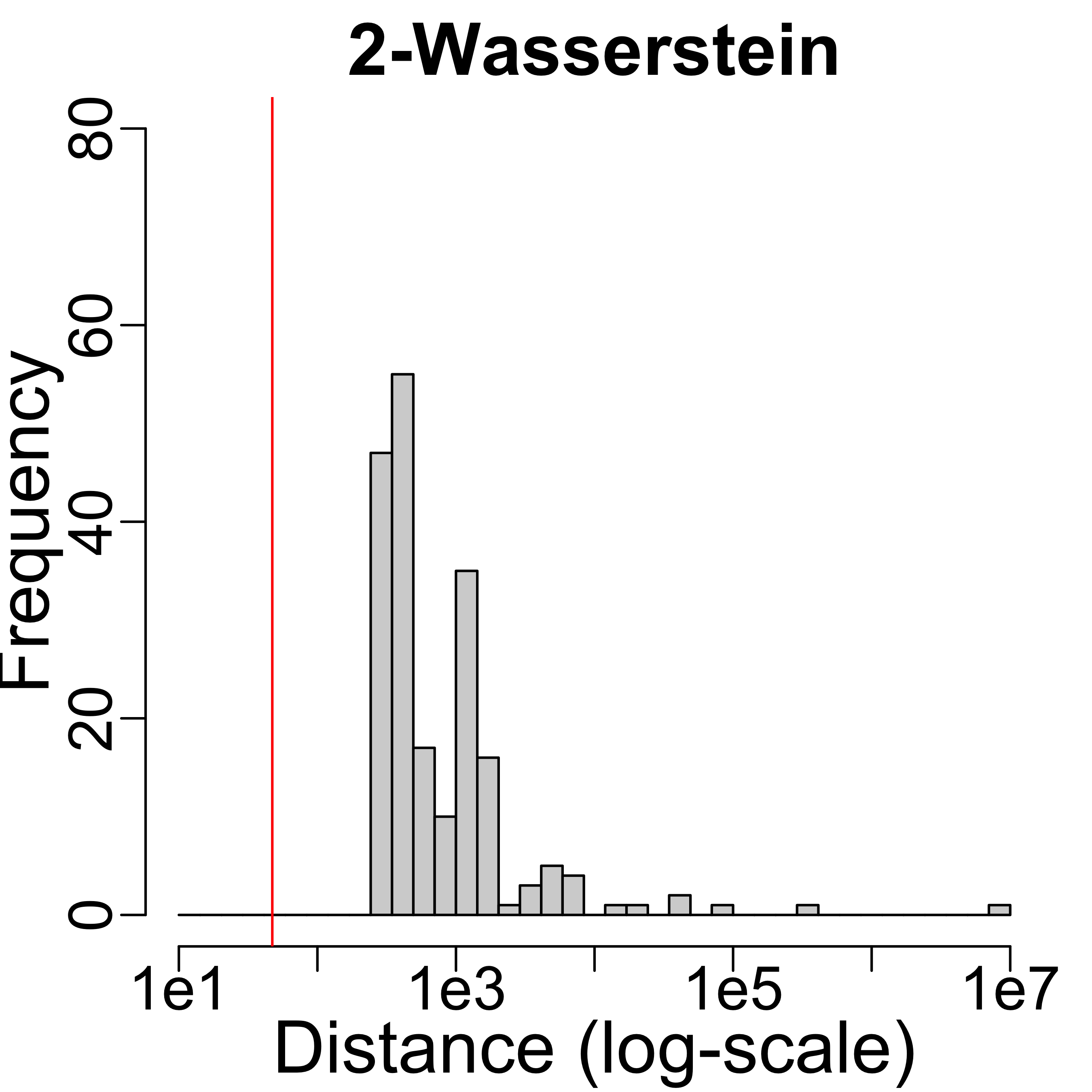
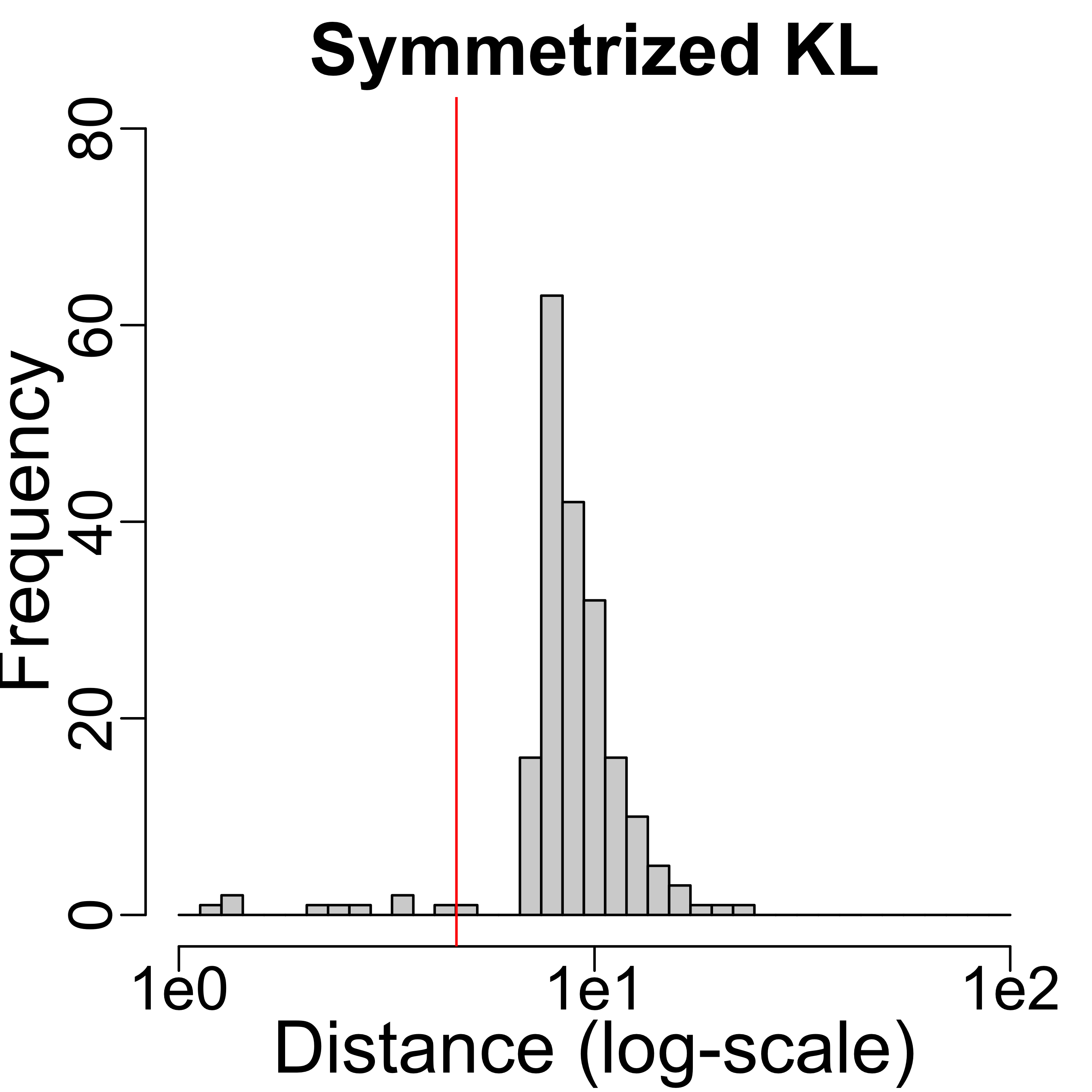
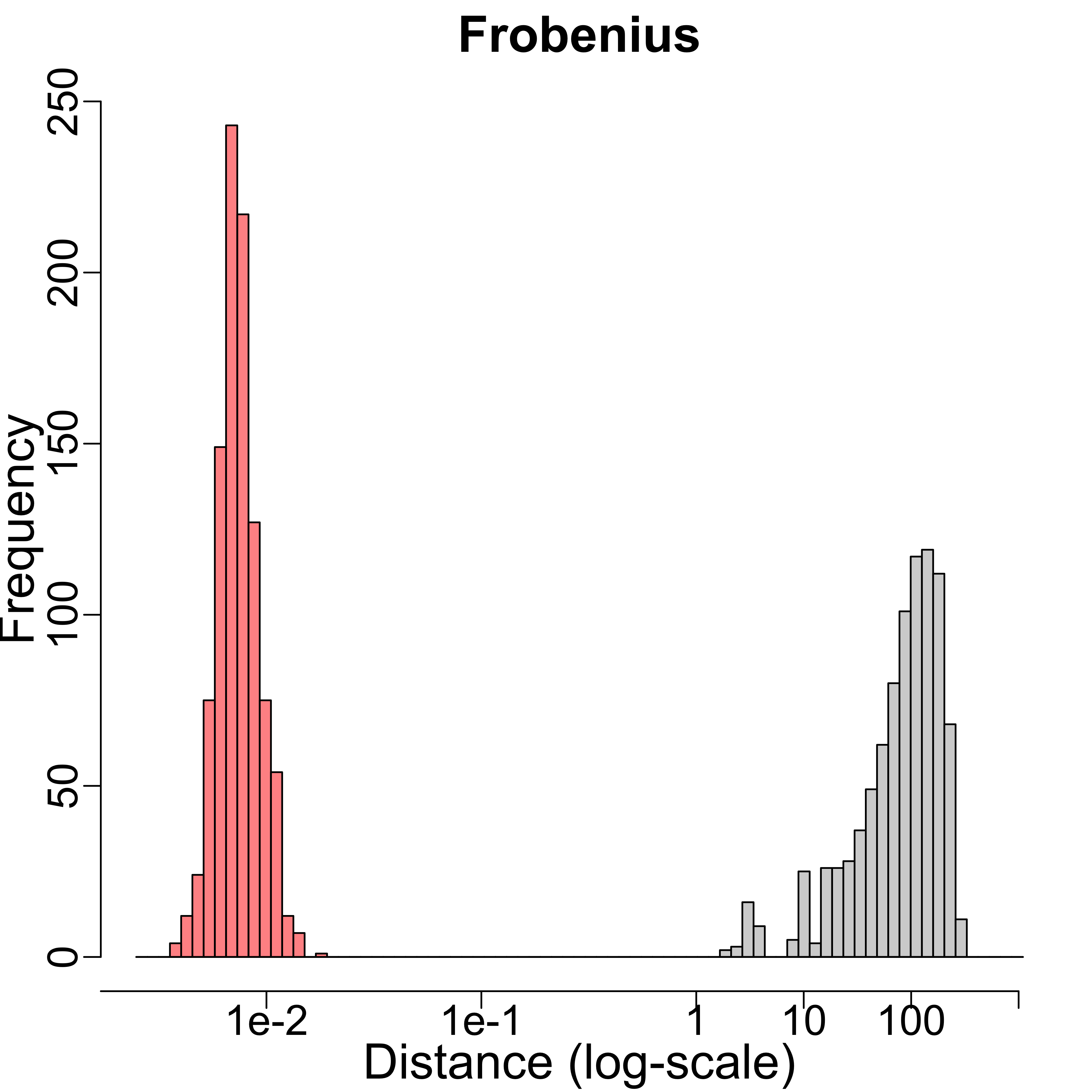
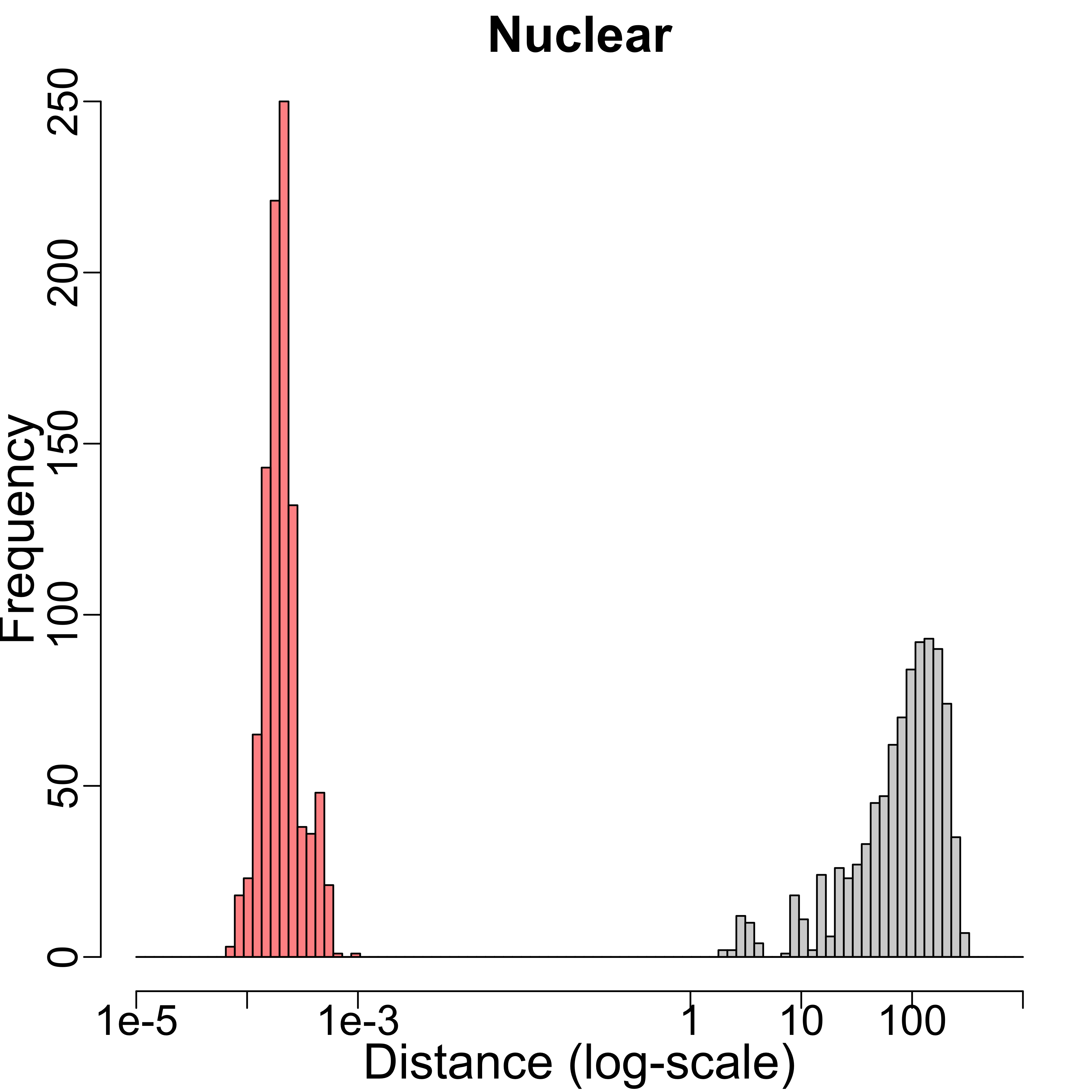
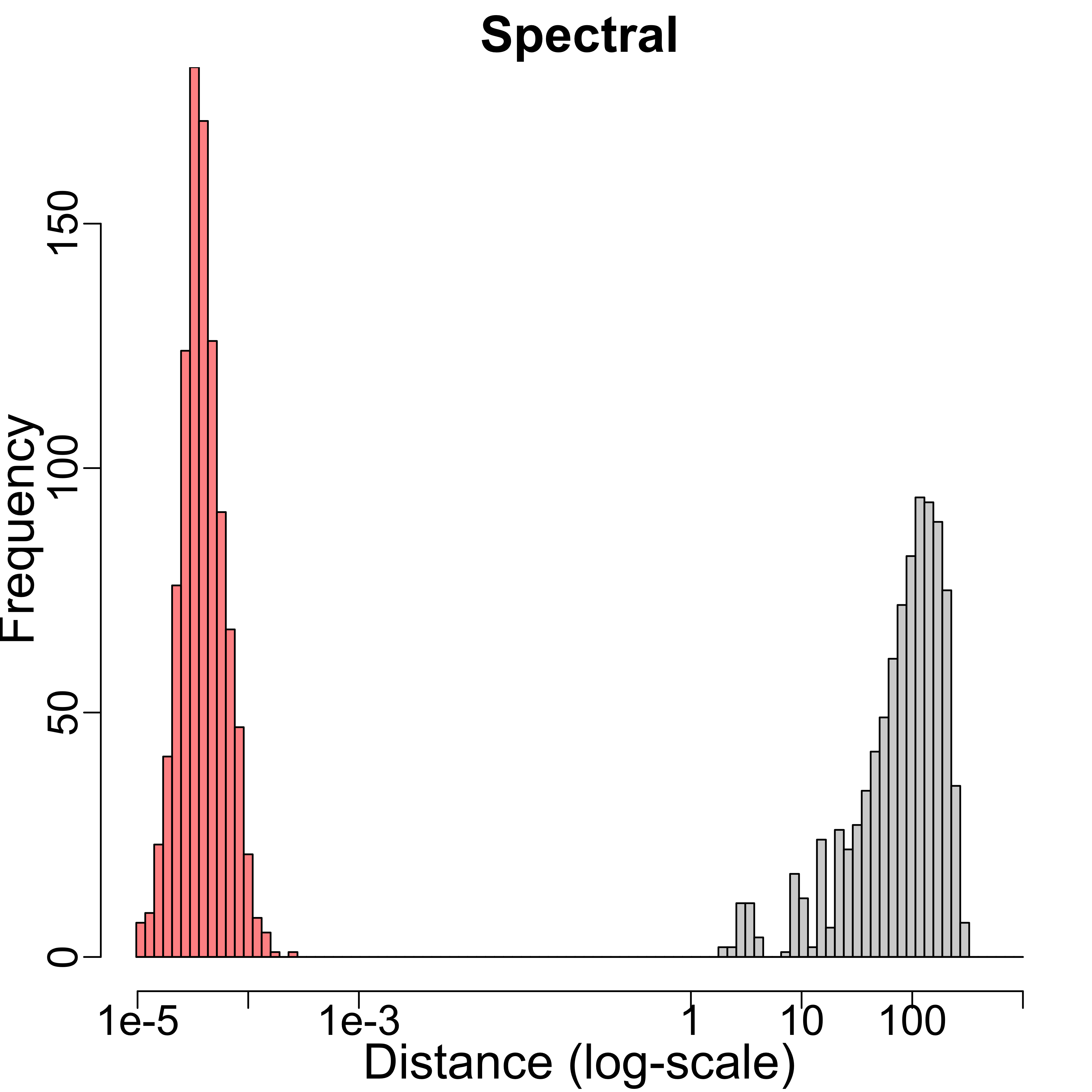
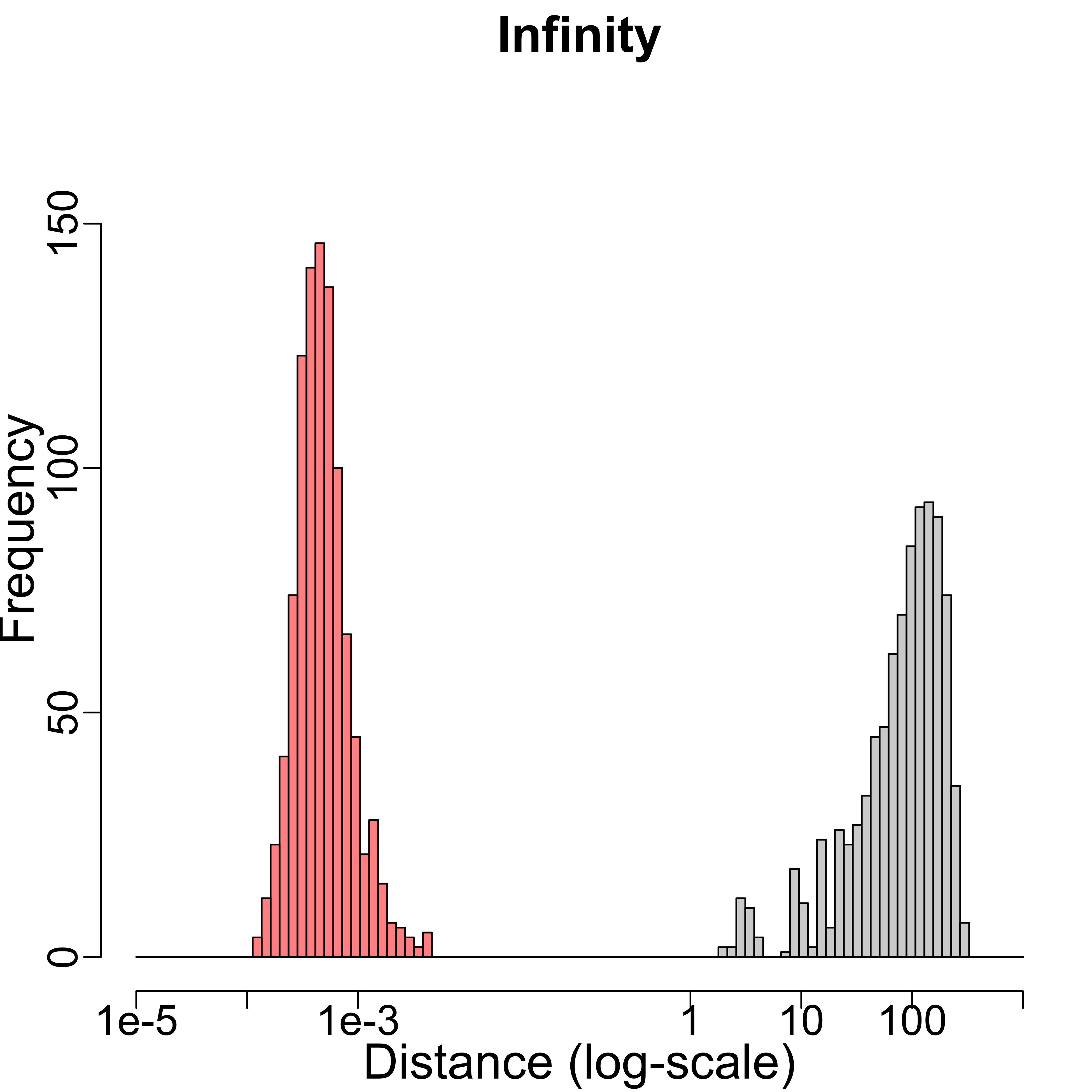
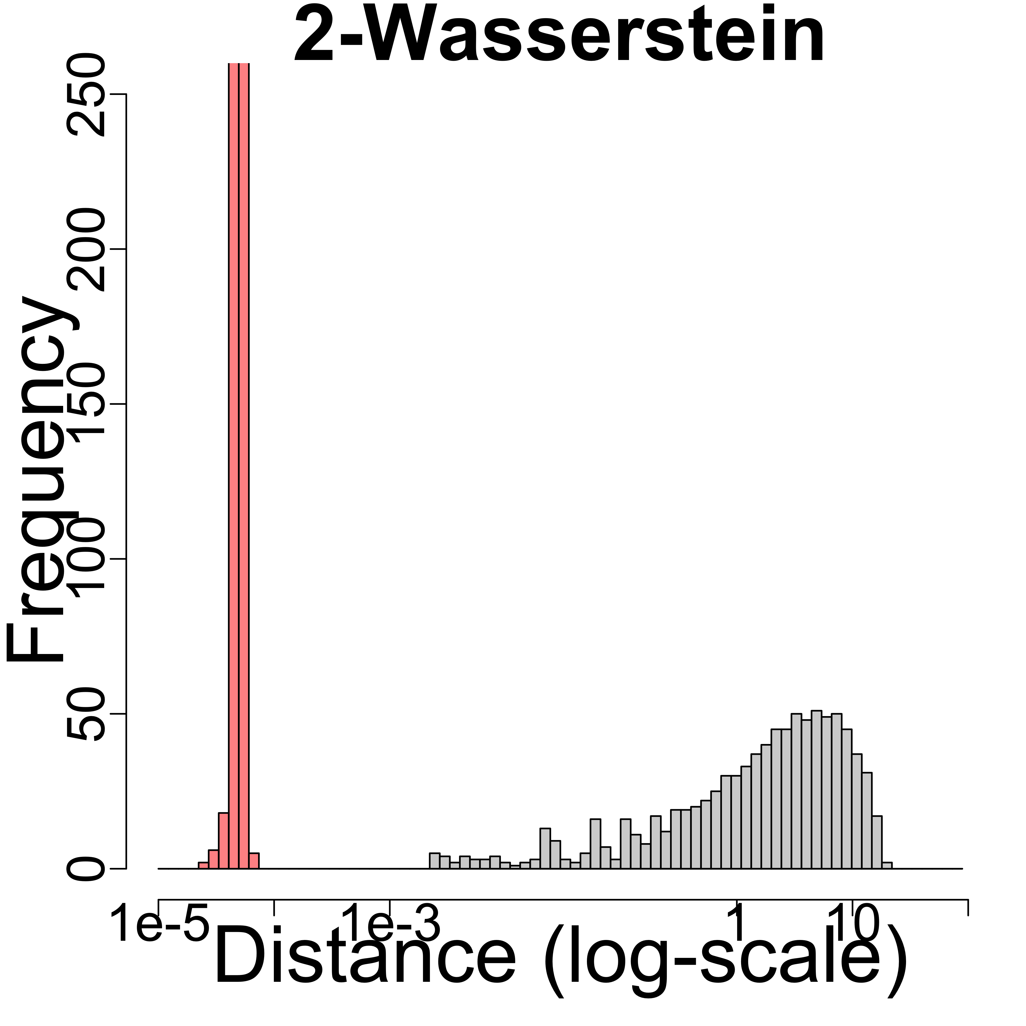
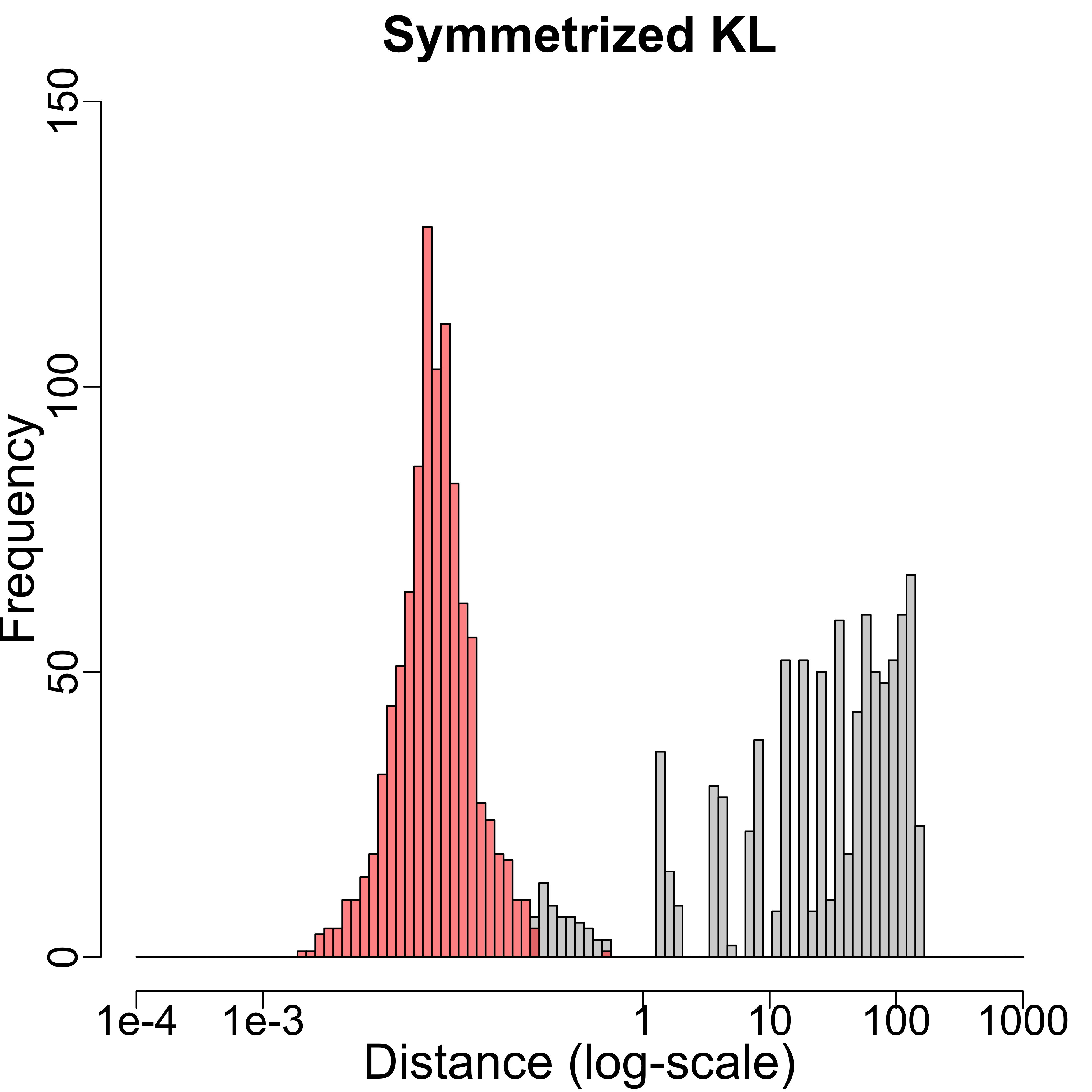
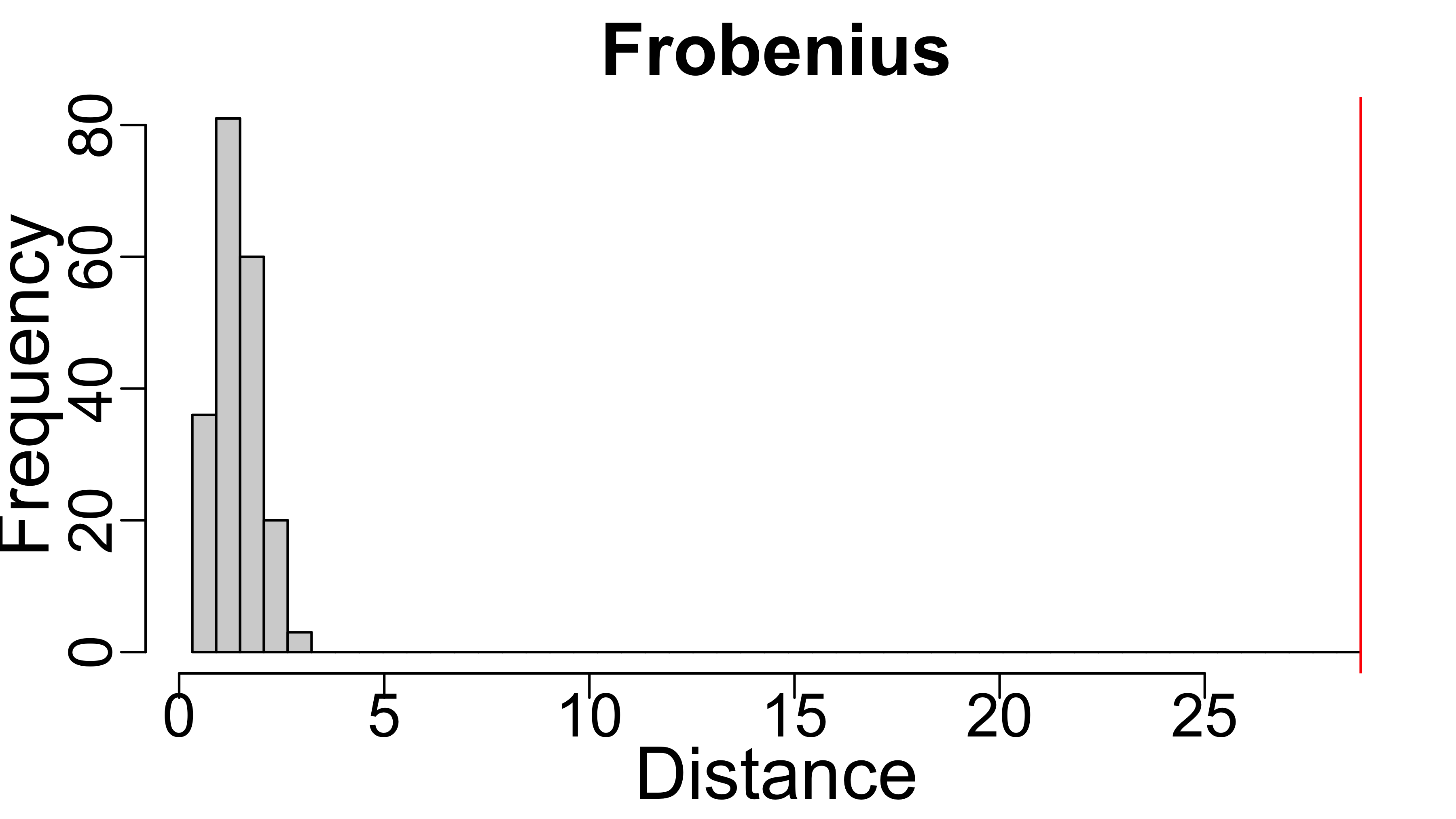
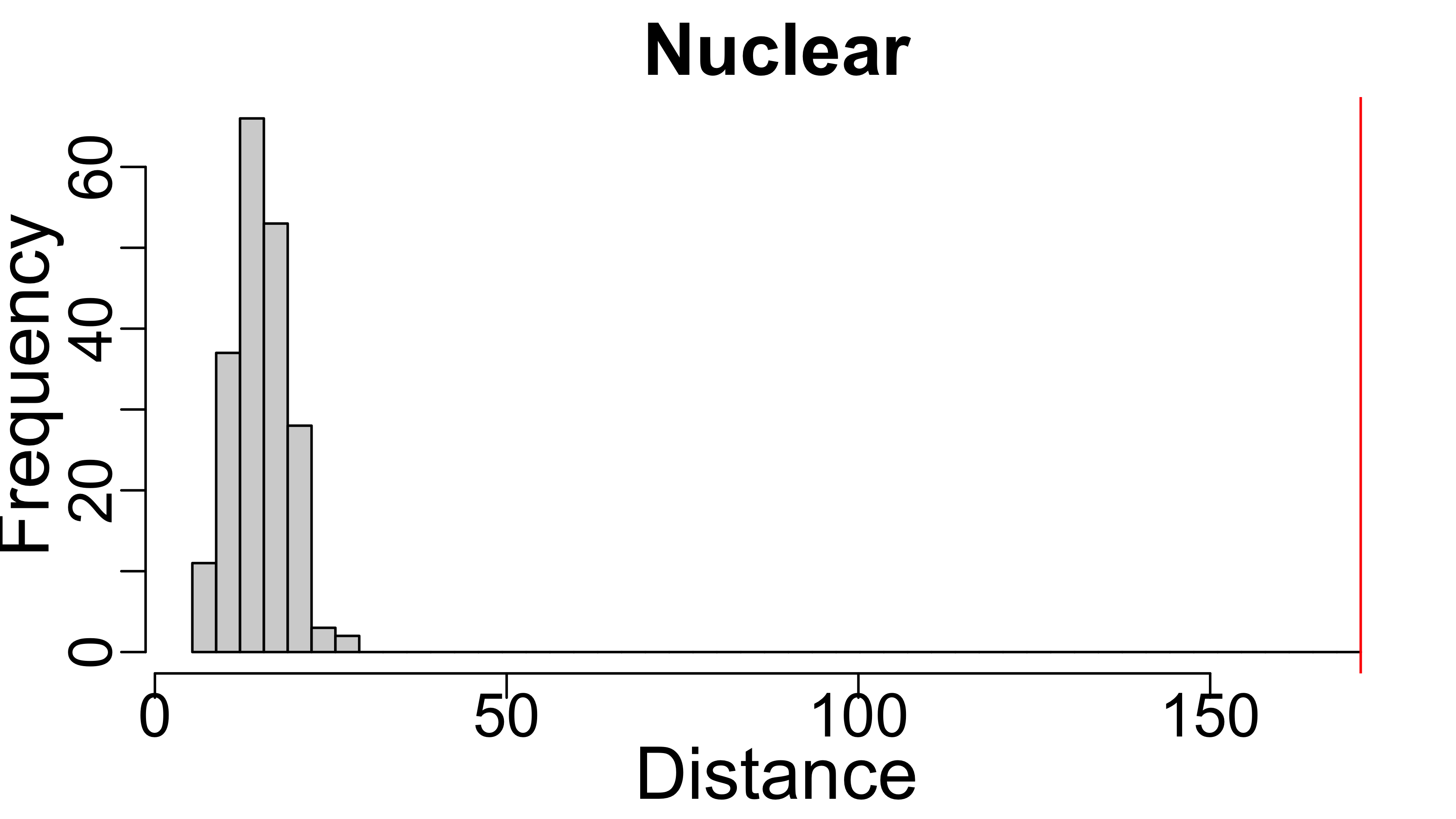
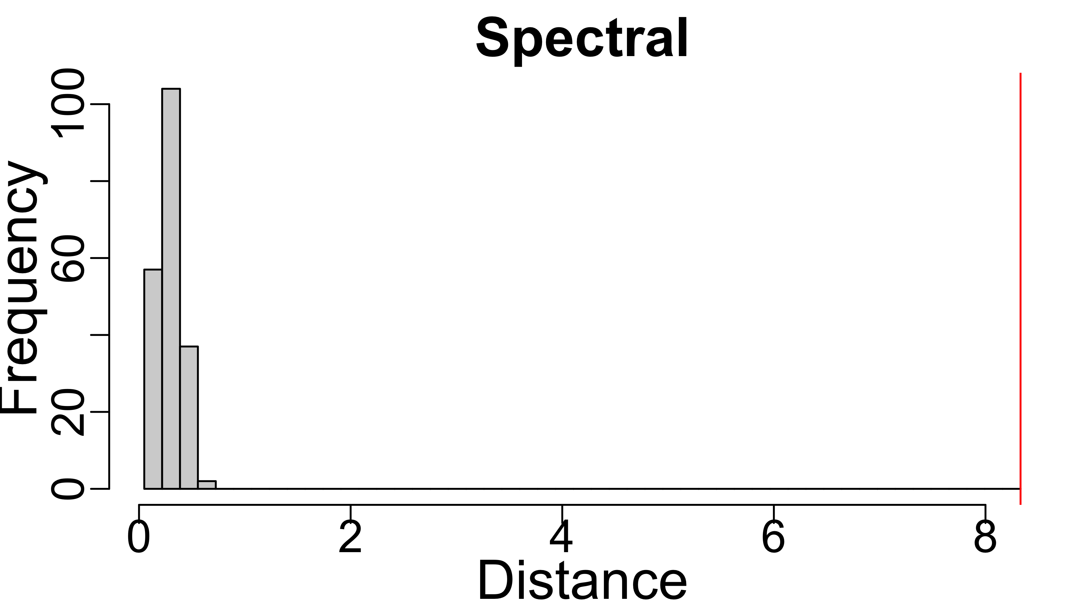
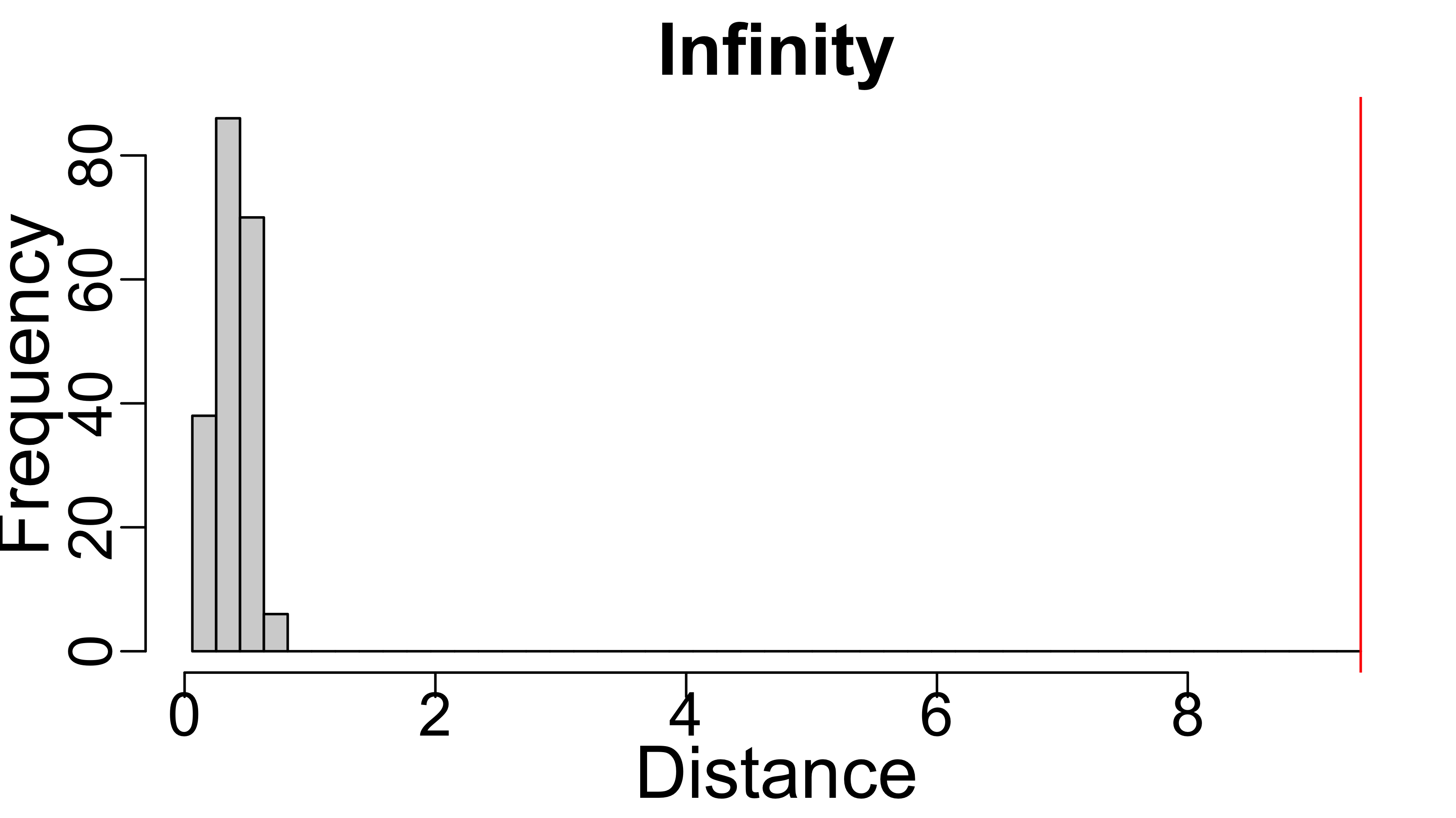
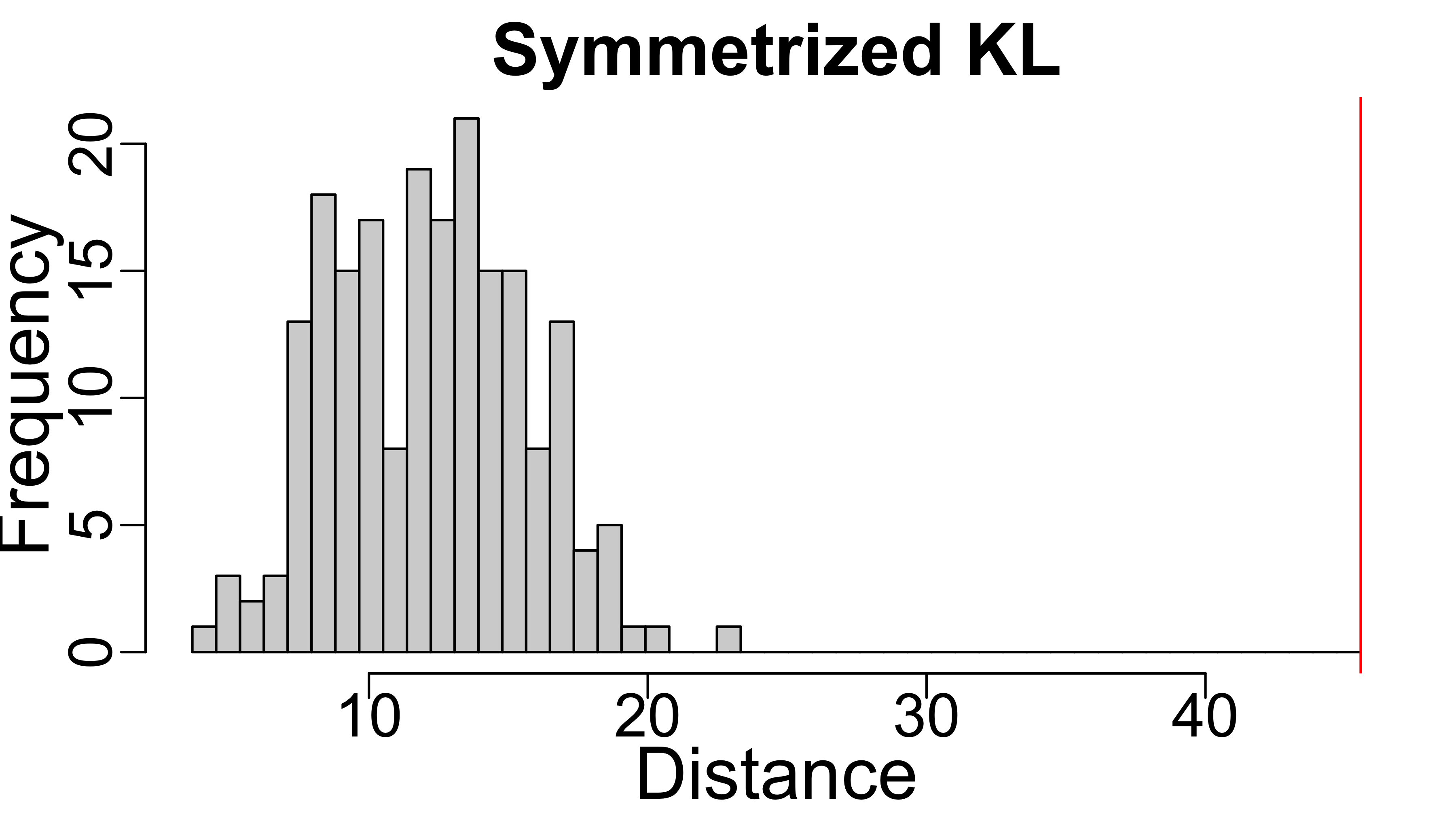
To assess qualitative interchangeability, we compared the 2-Wasserstein distance $d$ between the Gram matrices $k_{0}(X,X)$ and $k_{1}(\varepsilon^{*})(X,X)$ to the 2-Wasserstein distance between $k_{0}(X,X)$ and $k^{(r)}(X,X),$ where $k^{(r)}$ had the same functional form as $k_{0}$ but different hyperparameters. In Section 2.2, we argue that the 2-Wasserstein distance is a good default choice, as it corresponds to coordinate-wise differences in standard deviations. However, we emphasize that if a user has problem-specific knowledge that would make another distance $d$ more suitable, then our workflow can use this $d$ just as well. For example, if a user thinks that for any points $x_{1},x_{2}\in\mathbb{R}^{D}$, deviation in the covariance $\left|k_{1}(x_{1},x_{2})-k_{0}(x_{1},x_{2})\right|$ is meaningful in their problem, then they may want to consider $d$ as the infinity norm between Gram matrices. Here, we examine what what happens in all of our experiments when considering a number of matrix norms and statistical distances for $d$; in particular, we consider the Frobenius norm, nuclear norm, spectral norm, infinity norm, and symmetrized Kullback-Leibler distance.

In Figs. 13, 14, 15 and 18, we show the results of our histogram tests for qualitative interchangeability under these alternative $d$’s for our synthetic and heart-rate experiments. While the use of some $d$’s leads to the same conclusion as our use of the 2-Wasserstein distance in the main text, the use of the spectral norm or infinity norm can result in a different conclusion. In particular, in our synthetic extrapolation experiment and our heart rate example from the main text, we concluded that $k_{1}(\varepsilon^{*})$ and $k_{0}$ were qualitatively interchangeable (the red line sat to the left of the grey histograms); however, in Figs. 13 and 15, we see that the red line lies to the right of the grey histograms, which would lead us to reject qualitative interchangeability. We note that it is not surprising that kernels optimized according to Algorithm 2 deviation significantly in the spectral norm or infinity norm. This is because Algorithm 2 only constraints the spectral density of $k_{1}(\varepsilon^{*})$ to be close in a percentage-wise sense to the spectral density of $k_{0}$. If the spectral density of $k_{0}$ is large in an absolute sense – and it typically is for lower frequencies – then $k_{1}(\varepsilon^{*})$’s spectral density can have large deviations in an absolute sense. Large absolute deviations in the spectral density allow for large absolute deviations in the Gram matrices. As large absolute deviations in the Gram matrices is what the spectral and infinity norm measure, it is unsurprising that $\|k_{1}(\varepsilon^{*})(X,X)-k_{0}(X,X)\|_{spectral}$ and $\|k_{1}(\varepsilon^{*})(X,X)-k_{0}(X,X)\|_{infinity}$ are somewhat large. So, if a user decides that the spectral or infinity norm are appropriate in their context, we recommend using a constraint set in Algorithm 2 that better reflects this choice. E.g. one might constrain the density of $k_{1}(\varepsilon^{*})$ to be close in both a percentage and absolute sense.

Our CO₂ modeling example and MNIST example do not use the stationary constraints from Algorithm 2. We see in Figs. 16 and 17 that under all alternative choices of $d$ we consider here (including the spectral and infinity norms), we reach the same conclusions about qualitative interchangeability as we did under the 2-Wasserstein distance.

Figure 13: Extra hyperparameter uncertainty histograms for our synthetic extrapolation example in Section 2.3 in which we find find non-robustness. We compare the difference between $k_{0}$ and $k_{1}(\varepsilon^{*})$ (red) to bootstrapped hyperparameter uncertainty (gray) in several distances.

Figure 14: Extra hyperparameter uncertainty histograms for our synthetic interpolation example in Section 2.3 in which we find do not find non-robustness. We compare the difference between $k_{0}$ and $k_{1}(\varepsilon^{*})$ (red) to bootstrapped hyperparameter uncertainty (gray) in several distances.

Figure 15: Extra hyperparameter uncertainty histograms for our heart rate experiment in Section 3 in which we find non-robustness. We compare the difference between $k_{0}$ and $k_{1}(\varepsilon^{*})$ (red) to bootstrapped hyperparameter uncertainty (gray) in several distances.

Figure 16: Extra hyperparameter uncertainty histograms for our Mauna Loa experiment in Section 4 in which we find non-robustness. We compare the difference between $k_{0}$ and $k_{1}(\varepsilon^{*})$ (red) to bootstrapped hyperparameter uncertainty (gray) in several distances.

Figure 17: Extra hyperparameter uncertainty histograms for our MNIST experiment in Section 5 in which we find non-robustness. We compare the difference between $k_{0}$ and $k_{1}(\varepsilon^{*})$ (red) to bootstrapped hyperparameter uncertainty (gray) in several distances. Note, distances are plotted on the log-scale.

Figure 18: Extra hyperparameter uncertainty histograms for our additional heart rate experiment in Appendix C in which we to find non-robustness. We compare the difference between $k_{0}$ and $k_{1}(\varepsilon^{*})$ (red) to bootstrapped hyperparameter uncertainty (gray) in several distances.

References

- Andrews et al., (1972) Andrews, D. F., Bickel, P. J., Hampel, F. R., Huber, P. J., Rogers, W. H., and Tukey, J. W. (1972). Robust estimates of location: Survey and advances. Technical report, Princeton University.
- Benton et al., (2019) Benton, G. W., Maddox, W. J., Salkey, J. P., Albinati, J., and Wilson, A. G. (2019). Function-space distribution over kernels. In Advances in Neural Information Processing Systems (NeurIPS).
- Berger, (2000) Berger, J. O. (2000). Bayesian Robustness, pages 1–32. Springer New York, New York, NY.
- Berger et al., (1994) Berger, J. O., Moreno, E., Pericchi, L. R., Bayarri, M. J., Bernardo, J. M., Cano, J. A., De la Horra, J., Martín, J., Ríos-Insúa, D., Betrò, B., Dasgupta, A., Gustafson, P., Wasserman, L., Kadane, J. B., Srinivasan, C., Lavine, M., O’Hagan, A., Polasek, W., Robert, C. P., Goutis, C., Ruggeri, F., Salinetti, G., and Sivaganesan, S. (1994). An overview of robust Bayesian analysis. Test, 3(1):5 – 124.
- Bevilacqua et al., (2019) Bevilacqua, M., Faouzi, T., Furrer, R., and Porcu, E. (2019). Estimation and prediction using generalized Wendland covariance functions under fixed domain asymptotics. Annals of Statistics, 47(2).
- Bogunovic et al., (2018) Bogunovic, I., Scarlett, J., Jegelka, S., and Cevher, V. (2018). Adversarially robust optimization with Gaussian processes. In Advances in Neural Information Processing Systems (NeurIPS).
- Bradbury et al., (2018) Bradbury, J., Frostig, R., Hawkins, P., Johnson, M. J., Leary, C., Maclaurin, D., Necula, G., Paszke, A., VanderPlas, J., Wanderman-Milne, S., and Zhang, Q. (2018). JAX: composable transformations of Python+NumPy programs.
- Cardelli et al., (2019) Cardelli, L., Kwiatkowska, M., Laurenti, L., and Patane, A. (2019). Robustness guarantees for Bayesian inference with Gaussian processes. In AAAI Conference on Artificial Intelligence.
- Cheng et al., (2020) Cheng, L.-F., Dumitrascu, B., Darnell, G., Chivers, C., Draugelis, M., Li, K., and Engelhardt, B. E. (2020). Sparse multi-output Gaussian processes for online medical time series prediction. BMC Medical Informatics and Decision Making, 20(1):152 – 174.
- Colopy et al., (2016) Colopy, G. W., Pimentel, M. A. F., Roberts, S. J., and Clifton, D. A. (2016). Bayesian Gaussian processes for identifying the deteriorating patient. In 2016 38th Annual International Conference of the IEEE Engineering in Medicine and Biology Society (EMBC).
- de G. Matthews et al., (2018) de G. Matthews, A. G., Hron, J., Rowland, M., Turner, R. E., and Ghahramani, Z. (2018). Gaussian process behaviour in wide deep neural networks. In International Conference on Learning Representations (ICLR).
- Duvenaud, (2014) Duvenaud, D. (2014). Automatic model construction with Gaussian processes. PhD thesis, University of Cambridge.
- Duvenaud et al., (2013) Duvenaud, D., Lloyd, J. R., Grosse, R., Tenenbaum, J. B., and Ghahramani, Z. (2013). Structure discovery in nonparametric regression with compositional kernel search. In Proceedings of the 30th International Conference on Machine Learning (ICML).
- Ferrari and Dunson, (2020) Ferrari, F. and Dunson, D. B. (2020). Identifying main effects and interactions among exposures using Gaussian processes. Annals of Applied Statistics, 14(4):1743 – 1758.
- Fidler et al., (2017) Fidler, R. L., Pelter, M. M., Drew, B. J., Palacios, J. A., Bai, Y., Stannard, D., Aldrich, J. M., and Hu, X. (2017). Understanding heart rate alarm adjustment in the intensive care units through an analytical approach. PLoS One, 12(11):1 – 10.
- (16) Futoma, J., Hariharan, S., and Heller, K. (2017a). Learning to detect sepsis with a multitask Gaussian process RNN classifier. In Proceedings of the 34th International Conference on Machine Learning (ICML), volume 70.
- (17) Futoma, J., Hariharan, S., Heller, K., Sendak, M., Brajer, N., Clement, M., Bedoya, A., and O’Brien, C. (2017b). An improved multi-output Gaussian process RNN with real-time validation for early sepsis detection. In Proceedings of the 2nd Machine Learning for Healthcare Conference (MLHC).
- Gabry et al., (2019) Gabry, J., Simpson, D., Vehtari, A., Betancourt, M., and Gelman, A. (2019). Visualization in Bayesian workflow. Journal of the Royal Statistical Society: Series A (Statistics in Society), 182(2):389 – 402.
- Giordano et al., (2021) Giordano, R., Liu, R., Jordan, M. I., and Broderick, T. (2021). Evaluating sensitivity to the stick breaking prior in Bayesian nonparametrics. arXiv preprint arXiv:2107.03584v2.
- Goldberger et al., (2000) Goldberger, A. L., Amaral, L. A. N., Glass, L., Hausdorff, J. M., Ivanov, P. C., Mark, R. G., Mietus, J. E., Moody, G. B., Peng, C.-K., and Stanley, H. (2000). PhysioBank, PhysioToolkit, and PhysioNet: Components of a new research resource for complex physiologic signals. Circulation, 101(23):e215 – e220.
- Goodfellow et al., (2015) Goodfellow, I. J., Shlens, J., and Szegedy, C. (2015). Explaining and harnessing adversarial examples. In International Conference on Learning Representations (ICLR).
- Gustafson, (1996) Gustafson, P. (1996). Local sensitivity of posterior expectations. Annals of Statistics, 24(1):174 – 195.
- Hernández-Lobato et al., (2011) Hernández-Lobato, D., Hernández-Lobato, J. M., and Dupont, P. (2011). Robust multi-class Gaussian process classification. In Advances in Neural Information Processing Systems (NeurIPS).
- Huber and Ronchetti, (2009) Huber, P. J. and Ronchetti, E. (2009). Robust Statistics. John Wiley and Sons, Inc.
- Huggins et al., (2020) Huggins, J. H., Kasprzak, M., Campbell, T., and Broderick, T. (2020). Validated variational inference via practical posterior error bounds. In Proceedings of the 19th International Conference on Artificial Intelligence and Statistics (AISTATS).
- Insua and Ruggeri, (2000) Insua, D. R. and Ruggeri, F. (2000). Robust Bayesian Analysis. Springer.
- Jylänki et al., (2011) Jylänki, P., Vanhatalo, J., and Vehtari, A. (2011). Robust Gaussian process regression with a Student-t likelihood. Journal of Machine Learning Research, 12(99):3227 – 3257.
- Keeling et al., (2005) Keeling, C. D., Piper, S. C., Bacastow, R. B., Wahlen, M., Whorf, T. P., Heimann, M., and Meijer, H. A. (2005). Atmospheric and exchange with the terrestrial biosphere and oceans from 1978 to 2000: Observations and carbon cycle implications. In A history of atmospheric and its effects on plants, animals, and ecosystems, pages 83–113. Springer.
- Kim and Ghahramani, (2008) Kim, H.-C. and Ghahramani, Z. (2008). Outlier robust Gaussian process classification. In Structural, Syntactic, and Statistical Pattern Recognition, pages 896 – 905.
- Kirchner and Bolin, (2021) Kirchner, K. and Bolin, D. (2021). Necessary and sufficient conditions for asymptotically optimal linear prediction of random fields on compact metric spaces. arXiv preprint arXiv:2005.08904v4.
- Lee et al., (2017) Lee, D., Mukhopadhyay, S., Rushwork, A., and Sahu, S. K. (2017). A rigorous statistical framework for spatio-temporal pollution predition and estimation of its long-term impact on health. Biostatistics, 2:370 – 385.
- Lee et al., (2018) Lee, J., Sohl-Dickstein, J., Pennington, J., Novak, R., Schoenholz, S., and Bahri, Y. (2018). Deep neural networks as Gaussian processes. In International Conference on Learning Representations (ICLR).
- Novak et al., (2020) Novak, R., Xiao, L., Hron, J., Lee, J., Alemi, A. A., Sohl-Dickstein, J., and Schoenholz, S. S. (2020). Neural tangents: Fast and easy infinite neural networks in python. In International Conference on Learning Representations (ICLR).
- Ranjan et al., (2016) Ranjan, R., Huang, B., and Fatehi, A. (2016). Robust Gaussian process modeling using EM algorithm. Journal of Process Control, 42:125 – 136.
- Rasmussen and Williams, (2006) Rasmussen, C. E. and Williams, C. K. (2006). Gaussian Processes for Machine Learning. The MIT Press.
- Ren et al., (2021) Ren, B., Wu, X., Braun, D., Pillai, N., and Dominici, F. (2021). Bayesian modeling for exposure response curve via Gaussian processes: causal effects of exposure to air pollution on health outcomes. arXiv preprint arXiv:2105.0354v1.
- Reyna et al., (2019) Reyna, M., Josef, C., Jeter, R., Shashikumar, S., Moody, B., Westover, M., Sharm, A., Nemati, S., and Clifford, G. (2019). Early Prediction of Sepsis from Clinical Data – the PhysioNet Computing in Cardiology Challenge 2019 (version 1.0.0).
- Solly, (2019) Solly, M. (2019). Carbon dioxide levels reach highest point in human history. Smithsonian Magazine.
- Stein, (1993) Stein, M. L. (1993). A simple condition for asymptotic optimality of linear predictions of random fields. Statistics and Probability Letters, 17.
- Teckentrup, (2020) Teckentrup, A. L. (2020). Convergence of Gaussian process regression with estimated hyper-parameters and applications in Bayesian inverse problems. SIAM/ASA Journal on Uncertainty Quantification, 8:1310–1337.
- van der Vaart and van Zanten, (2011) van der Vaart, A. and van Zanten, H. (2011). Information rates of nonparametric Gaussian process methods. Journal of Machine Learning Research, 12:2095–2119.
- Wang and Jing, (2021) Wang, W. and Jing, B.-Y. (2021). Convergence of Gaussian process regression: Optimality, robustness, and relationship with kernel ridge regression. arXiv preprint arXiv:2104.09778v1.
- Wilson and Adams, (2013) Wilson, A. G. and Adams, R. P. (2013). Gaussian process kernels for pattern discovery and extrapolation. In Proceedings of the 30th International Conference on Machine Learning (ICML).
- Wilson et al., (2016) Wilson, A. G., Hu, Z., Salakhutdinov, R., and Xing, E. P. (2016). Deep kernel learning. In Proceedings of the 19th International Conference on Artificial Intelligence and Statistics (AISTATS).
- Wynne et al., (2021) Wynne, G., Briol, F.-X., and Girolami, M. (2021). Convergence guarantees for Gaussian process means with misspecified likelihoods and smoothness. Journal of Machine Learning Research, 22(123):1 – 40.