Attention-based Partial Face Recognition

Abstract

Photos of faces captured in unconstrained environments, such as large crowds, still constitute challenges for current face recognition approaches as often faces are occluded by objects or people in the foreground. However, few studies have addressed the task of recognizing partial faces. In this paper, we propose a novel approach to partial face recognition capable of recognizing faces with different occluded areas. We achieve this by combining attentional pooling of a ResNet’s intermediate feature maps with a separate aggregation module. We further adapt common losses to partial faces in order to ensure that the attention maps are diverse and handle occluded parts. Our thorough analysis demonstrates that we outperform all baselines under multiple benchmark protocols, including naturally and synthetically occluded partial faces. This suggests that our method successfully focuses on the relevant parts of the occluded face.

Index Terms—  Partial Face Recognition, Biometrics, Attention

1 Introduction

State-of-the-art Face Recognition (FR) approaches [1, 2, 3, 4] achieve satisfying performance under controlled imaging conditions, such as frontal faces, manually aligned images, regular expressions, and consistent illuminations. However, these requirements are often not fulfilled in many practical scenarios due to ineffectual control over the subjects and environments, resulting in partially visible faces. As illustrated in Figure 1, there are multiple examples for partial faces occurring in real-life scenarios: faces with extreme head poses causing face parts to become invisible; faces with intense illuminations or saturations provoking vanishing face details; faces in the background being obstructed by foreground objects or persons; faces at the edge of the image being cut off.

Fig. 1: Examples of partial faces ocurring in the LFW dataset [5].

After face detection, typical FR approaches for holistic faces use Convolutional Neural Networks to embed faces into a deep feature space, in which face pairs are considered genuine if their feature distance is lower than a threshold. For partial faces, however, partial face detection algorithms [6, 7, 8] are required to detect face parts even when the face is occluded, yielding a face with an arbitrary resolution. Therefore, partial FR approaches need to be capable of either handling arbitrary input resolutions [9, 10, 11, 12, 13] or tolerate that the information is only present in a small area within the input [14, 15]. Moreover, to compare partial with holistic faces, it is desirable to design a network performing well for both faces.

In our work, we propose an approach to partial FR using fixed-size images. The extracted face patches are normalized and zero-padded to match the input resolution. Hence, the face patch is not deformed yet centered, which causes the loss of any spatial information. To compensate for this information loss, we predict attention maps capable of focusing on their respective region of interest independent of their positions. Using attentional pooling followed by aggregation, we obtain a single feature vector robust against the lack of spatial information in face patches.

The contributions of our work can be summed up as follows:

• On the example of a ResNet [16], we propose an extension that utilizes attentional pooling with an aggregation network and is trained with two popular losses adapted for partial FR.

• In our exhaustive analysis covering multiple partial FR protocols, we show that our modifications substantially improve recognition performance and outperform the baselines for synthetically and naturally occluded partial faces.

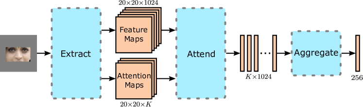
Fig. 2: Overview of our approach for partial FR.

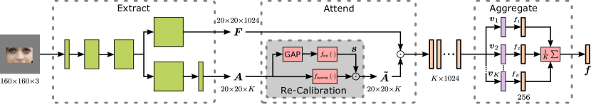
Fig. 3: Our proposed partial FR approach: A modified ResNet extracts feature maps $\boldsymbol{F}$ and attention maps $\boldsymbol{A}$. The re-calibrated attention maps $\boldsymbol{\tilde{A}}$ are used to pool $\boldsymbol{F}$ into $K$ feature descriptors $\boldsymbol{v}_{k}$. In the Aggregate module, $K$ independent fully connected layers transform every $\boldsymbol{v}_{k}$ into a joint feature space, in which the feature vectors $\boldsymbol{f}_{k}$ are averaged to obtain the final feature $\boldsymbol{f}$.

2 Related Work

Traditional partial FR approaches can be divided into region-based [17, 18, 19] and keypoint-based [9, 10, 11] approaches. Region-based approaches extract features from face patches, such as eyes, ears and nose [17], face halves [18], or the periocular region [19]. Keypoint-based approaches compute descriptors from face patches of arbitrary size. While Liao et al. [9] utilized Garbor Ternary Patterns as a descriptor and applied a sparse representation-based classification algorithm, Hu et al. [10] focused on SIFT features. Apart from SIFT, Weng et al. [11] also incorporated SURF and scale-invariant local binary pattern descriptors.

With emerging deep learning algorithms, He et al. [12] proposed a multiscale region-based CNN, which extracts a feature for every face patch at different scales. In order to cope with face patches of arbitrary size, He et al. [13] used dynamic feature learning to match local feature maps, which were obtained by a fully convolutional neural network. However, all previous approaches require overlapping patches during the matching. Thus, a cross-matching of partial faces of, e.g., the eye with the mouth region, is not possible.

In order to obtain a global face representation and focus on non-occluded face areas, utilizing a siamese network together with a predicted occlusion mask [14] or attention map [15] was proposed.

3 Methodology

3.1 Network Architecture

Figure 3 depicts our partial FR approach divided into three modules: Extract, Attend, and Aggregate. The Extract module extracts feature maps $\boldsymbol{F}\in\mathbb{R}^{20\times 20\times 1024}$ and attention maps $\boldsymbol{A}\in\mathbb{R}^{20\times 20\times K}$ from the input image with $K$ denoting the number of attention maps. In the Attend module, the feature maps are pooled into $K$ intermediate feature vectors using re-calibrated attention maps. The aggregation module maps these intermediate feature vectors into a joint feature space, in which the final feature vector $\boldsymbol{f}\in\mathbb{R}^{256}$ is obtained.

Table 1: The architecture of the Extract module. Residual blocks are shown in brackets, with the numbers of blocks stacked.

Block	Size	Layer
1	$80^{2}$	7$\times$7, 64, stride 2
2	$40^{2}$	3$\times$3 max pool, stride 2
		$\left[\begin{array}[]{c}\text{1$\times$1, \phantom{2}64}\\[-0.90005pt] \text{3$\times$3, \phantom{2}64}\\[-0.90005pt] \text{1$\times$1, 256}\end{array}\right]$$\times$3
3	$20^{2}$	$\left[\begin{array}[]{c}\text{1$\times$1, 128}\\[-0.90005pt] \text{3$\times$3, 128}\\[-0.90005pt] \text{1$\times$1, 512}\end{array}\right]$$\times$4
4	$20^{2}$	$\left[\begin{array}[]{c}\text{1$\times$1, \phantom{1}256}\\[-0.90005pt] \text{3$\times$3, \phantom{1}256}\\[-0.90005pt] \text{1$\times$1, 1024}\end{array}\right]$$\times$6	$\left[\begin{array}[]{c}\text{1$\times$1, \phantom{1}256}\\[-0.90005pt] \text{3$\times$3, \phantom{1}256}\\[-0.90005pt] \text{1$\times$1, 1024}\end{array}\right]$$\times$6
			1$\times$1, $K$

3.1.1 Extract

Inspired by [20], we utilize a truncated ResNet-50 architecture [16], which is concluded after the fourth block. Hence, we only perform three spatial downsamplings and obtain feature maps of size $20\times 20$, in which the regions are still well distinguishable. Unlike [20], we separate the ResNet after the third block to allow both branches to focus on their respective tasks. While we directly obtain $\boldsymbol{F}$ after the fourth ResNet block, we add an extra $1\times 1$ convolution with ReLU [21] activation function to obtain $\boldsymbol{A}$. The detailed architecture is summed up in Table 1.

The generated attention maps should fulfill the following two key attributes: 1) Attention maps should be mutually exclusive, i.e., different attention maps focus on different regions of a face image; 2) The attention maps’ activations should correlate with their respective region’s visibility.

Notably, the implicitly-defined attention map activations do not necessarily follow the same intuition as human-defined facial landmarks such as eyes or nose.

3.1.2 Attend

As in [20], the attention maps $\boldsymbol{A}$ need to be re-calibrated. Xie et al. [20] proposed the attentional pooling for set-based FR normalizing $\boldsymbol{A}$ separately over all images within a set, thereby ensuring that the respective information is extracted from the image with the largest activation in $\boldsymbol{A}$. For partial FR, however, we only consider a single image and expect different attention maps to be relevant depending on the region of the face, i.e., if the eyes are occluded, the corresponding attention maps should contain low activations. Thus, we propose to use a parameter-free re-calibration following the structure of [22]:

First, we normalize $\boldsymbol{A}$ by applying the sigmoid function $f_{\text{norm}}\left(\cdot\right)=\operatorname{sigmoid}\left(\cdot\right)$. In this way, every pixel in every attention map is normalized separately to $(0;1)$. Besides, we compute a vector $\boldsymbol{s}\in\mathbb{R}^{K}$ representing the importance of every attention map by applying Global Average Pooling (GAP) followed by $f_{\text{ex}}\left(\cdot\right)=\operatorname{softmax}\left(\cdot\right)$:

$$\boldsymbol{s}=f_{\text{ex}}\left(\frac{1}{20^{2}}\sum_{i,j}\boldsymbol{A}_{i,j,k}\right)$$ (1)

with the indices $i$, $j$, and $k$ denoting the pixel in the $i$-th row and $j$-th column of the $k$-th attention map. By incorporating GAP, we obtain global information of all attention maps and transform it into a probability distribution indicating the importance of the respective attention map using the softmax function. Next, we multiply the $k$-th self-normalized attention map $\boldsymbol{A}_{k}$ with its corresponding importance $s_{k}$ to obtain the final re-calibrated attention map $\boldsymbol{\tilde{A}}_{k}$:

$$\boldsymbol{\tilde{A}}_{k}=s_{k}\cdot\operatorname{sigmoid}\left(\boldsymbol{A}_{k}\right)$$ (2)

Hence, in our re-calibration, we combine local information within each attention map together with global information across the attention maps.

After re-calibration, we apply attentional pooling as in [20] to obtain $K$ feature descriptors $\boldsymbol{v}_{k}\in\mathbb{R}^{1024}$:

$$\boldsymbol{v}_{k}=\sum_{i,j}\boldsymbol{F}_{i,j,:}\odot\boldsymbol{\tilde{A}}_{i,j,k}$$ (3)

In this way, the $k$-th feature descriptor contains the information of $\boldsymbol{F}$ at the activation of the corresponding attention map $\boldsymbol{A}_{k}$.

3.1.3 Aggregate

We conclude our partial FR model with the Aggregate module. Since all feature descriptors $\boldsymbol{v}_{k}$ focus on different regions within $\boldsymbol{F}$ depending on their corresponding attention map $\boldsymbol{A}_{k}$, a direct aggregation is impossible. Thus, we map every $\boldsymbol{v}_{k}$ separately into a joint feature space $\boldsymbol{f}_{k}\in\mathbb{R}^{256}$ utilizing a single fully connected layer each. Note that as every $\boldsymbol{v}_{k}$ is in a different feature space, the weights are not shared. Since $\boldsymbol{f}_{k}$ encode identity information likewise, we compute the mean to obtain the final feature vector $\boldsymbol{f}\in\mathbb{R}^{256}$:

$$\boldsymbol{f}=\frac{1}{K}\sum\limits_{k}\boldsymbol{f}_{k}$$ (4)

3.2 Loss Functions

To train our model, we apply a weighted sum of three losses $\mathscr{L}$, which are described in the following:

$$\mathscr{L}=\ \lambda_{\text{wCE}}\mathscr{L}_{\text{wCE}}+\ \lambda_{\text{wDIV}}\mathscr{L}_{\text{wDIV}}+\lambda_{\text{REG}}\mathscr{L}_{\text{REG}}$$ (5)

with $\lambda_{\text{wCE}}$, $\lambda_{\text{wDIV}}$ and $\lambda_{\text{REG}}$ denoting hyperparameters to balance the losses, and $\mathscr{L}_{\text{REG}}$ is the $L^{2}$-norm of all trainable weights.

3.2.1 Weighted Cross-Entropy $\mathscr{L}_{\text{wCE}}$

To cope with some vectors $\boldsymbol{f}_{k}$ representing occluded regions and thus being less relevant, we propose a weighted softmax Cross-Entropy (CE) loss. As usual for CE losses, we add a fully connected layer to every feature vector $\boldsymbol{f}_{k}$ matching the number of classes in our training dataset. In this way, we obtain $K$ CE losses $\mathscr{L}_{\text{CE},k}$. To obtain our final weighted CE loss, we scale every $\mathscr{L}_{\text{CE},k}$ with its importance $s_{k}$ as computed in Equation 1:

$$\mathscr{L}_{\text{wCE}}=\sum\limits_{k}s_{k}\cdot\mathscr{L}_{\text{CE},k}$$ (6)

In this way, the network learns to emphasize attention maps representing visible face areas while mitigating the influence of attention maps representing occluded regions. Note that since the weights of the last fully connected layers are shared, every $\boldsymbol{f}_{k}$ is transformed equally, and thereby, we ensure that they encode identity information likewise, i.e., lie in the same feature space. Moreover, due to the high number of classes in the training dataset, $\boldsymbol{f}_{k}$ act as bottleneck layers improving our network’s generalization.

3.2.2 Weighted Diversity Regularizer $\mathscr{L}_{\text{wDIV}}$

The diversity regularizer’s objective is to assure diversity within the attention maps as, without regularization, the network is prone to tend towards using only one attention map or generating $K$ identical attention maps. We apply an adaptation of the diversity regularizer from Xie et al. [20] to penalize the mutual overlap between different attention maps. First, every attention map $\boldsymbol{A}_{k}$ is self-normalized into a probability distribution $\boldsymbol{P}_{k}$ using the softmax function:

$$\boldsymbol{P}_{i,j,k}=\frac{\exp\left(\boldsymbol{A}_{i,j,k}\right)}{\sum\limits_{i,j}\exp\left(\boldsymbol{A}_{i,j,k}\right)}$$ (7)

Next, we compute their pixel-wise maximum of all $\boldsymbol{P}_{k}$ scaled with their respective $s_{k}$ and obtain the sum of all pixels. For mutually non-overlapping attention maps, this sum is close to 1, which allows computing the weighted diversity loss $\mathscr{L}_{\text{wDIV}}$ as follows:

$$\mathscr{L}_{\text{wDIV}}=1-\sum\limits_{i,j}\max_{k}\left(s_{k}\cdot\boldsymbol{P}_{i,j,k}\right)$$ (8)

4 Experiments

4.1 Training Details

Our training is divided into two steps. First, we pretrain the model on holistic faces for 20 epochs with ADAM optimizer [23] and a batch size of 50. However, instead of using the weighted CE as defined in Equation 6, we average all $\mathscr{L}_{\text{CE},k}$ and balance the losses by setting $\lambda_{\text{wCE}}=\lambda_{\text{wDIV}}=1$ and $\lambda_{\text{REG}}=5\cdot 10^{-5}$. We start with an initial learning rate of $0.05$ and divide it by $4$ every 6 epochs. As training dataset, we utilize VGG-Face2 [24], which comprises 3.3 M images of 8631 identities. Using the facial landmarks extracted with MTCNN [25], we align every face and crop it to a resolution of $160\times 160$ pixels. To improve generalization, we augment the faces by changing brightness, contrast and saturation, and perform left-right flipping with a probability of $50\,\%$. Moreover, dropout with $80\,\%$ keep probability is added after $\boldsymbol{v}_{k}$.

In a second step, we leverage that the model performs well on holistic faces and further finetune it on partial faces. As depicted in Figure 4 (left), we synthetically generate rectangular partial faces with an area between $10\,\%$ and $100\,\%$ with a probability of $80\,\%$. Since weights are now well-initialized, we finetune the model for 5 more epochs using an initial learning rate of 0.002 and decay it every 2 epochs. Moreover, we use the weighted CE loss $\mathscr{L}_{\text{wCE}}$ as in Equation 6. All remaining parameters are identical as during pretraining.

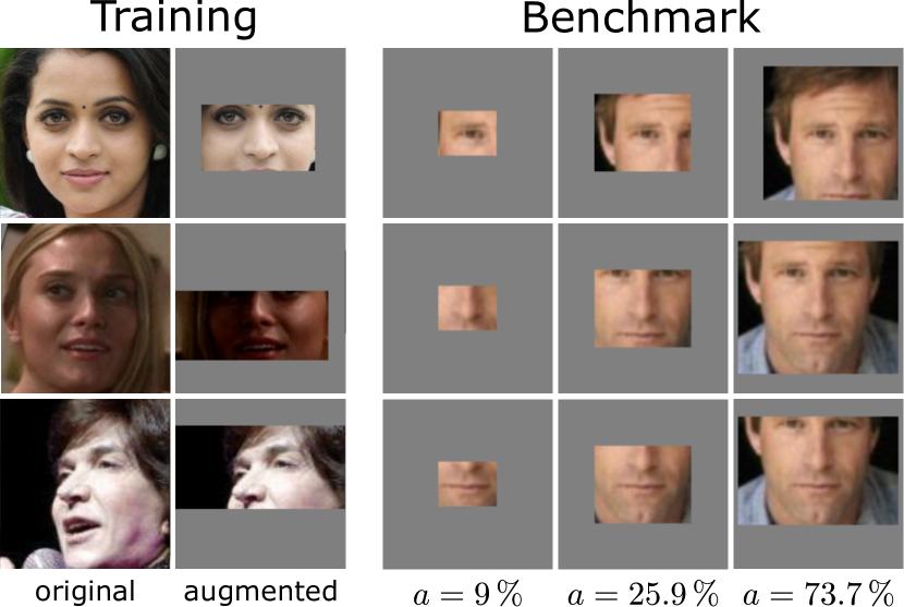
Fig. 4: Faces during finetuning before (first column) and after (second column) applying data augmentation (left). Generation of faces for our centered partial LFW protocol for different non-occluded areas $a$ (right).

Table 2: Effect of different parameters on the accuracy in $\%$ on the LFW and CPLFW dataset. Mean accuracies over nine non-occluded areas $a$ are reported for partial - holistic (e.g. mouth - holistic), partial - same (e.g. mouth - mouth), and partial - cross (e.g. mouth - nose).

					CPLFW	LFW
							non-centered: partial -			centered: partial -			#
$K$	Agg	$\mathscr{L}_{\text{wCE}}$	$f_{\text{ex}}$	$f_{\text{norm}}$	holistic	holistic	holistic	same	cross	holistic	same	cross	Params
ResNet-41					87.52	99.62	97.71	97.27	94.53	97.25	96.80	93.56	08.82 M
ResNet-50 (no finetune)					88.20	99.58	94.77	94.93	88.85	92.05	92.47	83.92	24.05 M
ResNet-50					87.80	99.60	97.75	97.36	94.80	95.48	94.72	89.60	24.05 M
5			no re-calibration		87.80	99.47	97.60	97.18	94.14	97.01	96.64	92.96	16.19 M
5			softmax	softmax	88.42	99.45	97.76	97.30	94.23	97.25	96.77	93.00	16.19 M
5			softmax	sigmoid	88.87	99.62	98.04	97.60	94.58	97.62	97.16	93.45	16.19 M
5	$\surd$		softmax	sigmoid	89.10	99.47	98.02	97.56	94.79	97.61	97.12	93.74	17.25 M
5	$\surd$	$\surd$	softmax	sigmoid	89.18	99.67	97.99	97.54	94.79	97.58	97.08	93.73	17.25 M
12			no re-calibration		88.03	99.63	97.74	97.28	94.38	97.17	96.63	93.06	16.20 M
12			softmax	softmax	88.10	99.50	97.61	97.11	94.43	96.77	96.24	92.68	16.20 M
12			softmax	sigmoid	89.13	99.62	97.99	97.61	94.62	97.54	97.03	93.44	16.20 M
12	$\surd$		softmax	sigmoid	89.08	99.60	98.02	97.56	94.85	97.60	97.08	93.86	19.09 M
12	$\surd$	$\surd$	softmax	sigmoid	88.97	99.70	98.03	97.66	94.90	97.64	97.16	93.87	19.09 M

4.2 Benchmark Details

We evaluate our approach on the synthetically-occluded partial Labeled Faces in the Wild (LFW) dataset , which is based on LFW [5]. To generate partial faces, we crop rectangular face patches of nine different areas ranging from $a=9\,\%$ to $a=73.7\,\%$ of the original face around three landmarks: left eye, nose, and mouth. Next, we either leave the cropped face patches at their initial location and fill the remaining image with zeros (non-centered) or move the patch to the center and zero-pad to match the input resolution (centered). Moreover, we utilize the CPLFW [26] dataset, which contains naturally occurring occlusion due to extreme head poses. As distance measure, we utilize the cosine distance of the features $\boldsymbol{f}$.

Fig. 5: Accuracy on the LFW dataset for $K=12$, $f_{\text{ex}}=\operatorname{sigmoid}$, and $f_{\text{norm}}=\operatorname{softmax}$ with Aggregate and $\mathscr{L}_{\text{wCE}}$ on the centered partial - cross protocol dependent on the non-occluded area $a$.

4.3 Baselines

We compare our approach with a standard ResNet-50 and a ResNet-41, which is obtained by removing the last block of a ResNet-50 and, thus, has the same depth as our approach. Both are trained on softmax CE loss and with identical parameters as in subsection 4.1. We also train without the Aggregate module (Agg) by averaging all $K$ normalized attention maps $\boldsymbol{\tilde{A}}_{k}$ to obtain a global attention map. Then, attentional pooling is applied only for the global attention map followed by a single bottleneck layer to obtain the feature vector.

4.4 Results

Table 2 depicts the aggregated accuracies for different benchmark protocols on the LFW dataset. When considering a ResNet-50 (no finetune), which was never exposed to partial faces during training, we can observe that standard FR models are very susceptible to partial faces. By finetuning on partial faces, the model performs better on the partial protocols. While ResNet-50 outperforms ResNet-41 on the non-centered protocols, it is inferior on the centered protocols. We believe that this is due to ResNet-50 containing more trainable parameters. Thus, it is more prone to overfit on the spatial information present during training, since centering was not part of our data augmentation.

Our ablation study shows that the re-calibration with $f_{\text{ex}}$ $=\operatorname{sigmoid}$ and $f_{\text{norm}}$$\,=\,$$\operatorname{softmax}$ is crucial for a well-performing model. The number of attention maps $K$ only has a minor influence, yet models with $K$$\,=\,$$12$ tend to have superior performance. The Aggregate module and weighted CE loss $\mathscr{L}_{\text{wCE}}$ improve the performance, especially in the partial - cross protocols. For naturally occurring occlusions as in CPLFW, our model also improves the baseline. Besides, our approach further boosts the accuracy on the holistic LFW benchmark, suggesting that our Attend and Aggregate modules combined with partial faces as data augmentation assist generalization. Overall, our approach to partial FR outperforms all baselines while comprising fewer parameters than ResNet-50.

In Figure 5, we illustrate the influence of the non-occluded area $a$ of partial faces in the centered: partial - cross protocol. While the accuracy when recognizing Left Eye - Right Eye is only slightly affected by $a$, the scenario of verifying whether Mouth - Left Eye belong to the same identity is considered most challenging. Overall, we can conclude that our model is more robust compared to the baseline for all centered: partial - cross cases.

5 Conclusion

In this paper, we propose a CNN for partial FR consisting of three modules: 1) Extract to predict feature maps and attention maps using a truncated ResNet-50; 2) Attend to re-calibrate the attention maps and perform attentional pooling; 3) Aggregate to fuse the feature information into one global feature vector.

Our exhaustive analysis demonstrates that our approach outperforms all baselines and provides satisfying results for the arguable more challenging partial - cross protocols (e.g. mouth - nose). These results suggest that our model successfully transforms any arbitrary face patch into a joint feature space, in which even the matching of non-overlapping face patches is possible.

References

- [1] W. Liu, Y. Wen, Z. Yu, M. Li, B. Raj, and L. Song, “SphereFace: Deep Hypersphere Embedding for Face Recognition,” in IEEE Conference on Computer Vision and Pattern Recognition (CVPR), 2017, pp. 6738–6746.
- [2] H. Wang, Y. Wang, Z. Zhou, X. Ji, D. Gong, J. Zhou, Z. Li, and W. Liu, “CosFace: Large Margin Cosine Loss for Deep Face Recognition,” in Proceedings of the IEEE Conference on Computer Vision and Pattern Recognition (CVPR), 2018, pp. 5265–5274.
- [3] J. Deng, J. Guo, N. Xue, and S. Zafeiriou, “ArcFace: Additive Angular Margin Loss for Deep Face Recognition,” in Proceedings of the IEEE Conference on Computer Vision and Pattern Recognition (CVPR), 2019, pp. 4690–4699.
- [4] Y. Kim, W. Park, M.C. Roh, and J. Shin, “GroupFace: Learning Latent Groups and Constructing Group-based Representations for Face Recognition,” in Proceedings of the IEEE/CVF Conference on Computer Vision and Pattern Recognition (CVPR), 2020, pp. 5621–5630.
- [5] E. G. Huang, G. B. Learned-Miller, “Labeled Faces in the Wild: Updates and New Reporting Procedures,” Tech. Rep. UM-CS-2014-003, University of Massachusetts, Amherst, May 2014.
- [6] M. Opitz, G. Waltner, G. Poier, H. Possegger, and H. Bischof, “Grid Loss: Detecting Occluded Faces,” in European Conference on Computer Vision (ECCV), 2016.
- [7] U. Mahbub, V.M. Patel, D. Chandra, B. Barbello, and R. Chellappa, “Partial Face Detection for Continuous Authentication,” in IEEE International Conference on Image Processing (ICIP). IEEE, 2016, pp. 2991–2995.
- [8] Y. Chen, L. Song, Y. Hu, and R. He, “Adversarial Occlusion-aware Face Detection,” in IEEE 9th International Conference on Biometrics Theory, Applications and Systems (BTAS). IEEE, 2018, pp. 1–9.
- [9] S. Liao, A. K. Jain, and S. Z. Li, “Partial Face Recognition: An Alignment Free Approach,” IEEE Transactions on Pattern Analysis and Machine Intelligence, vol. 35, no. 5, pp. 1193–1205, 2012.
- [10] J. Hu, J. Lu, and Y.P. Tan, “Robust partial face recognition using instance-to-class distance,” in Visual Communications and Image Processing (VCIP). IEEE, 2013, pp. 1–6.
- [11] R. Weng, J. Lu, and Y.P. Tan, “Robust Point Set Matching for Partial Face Recognition,” IEEE Transactions on Image Processing, vol. 25, no. 3, pp. 1163–1176, 2016.
- [12] L. He, H. Li, Q. Zhang, Z. Sun, and Z. He, “Multiscale Representation for Partial Face Recognition Under Near Infrared Illumination,” in IEEE 8th International Conference on Biometrics Theory, Applications and Systems (BTAS). IEEE, 2016, pp. 1–7.
- [13] L. He, H. Li, Q. Zhang, and Z. Sun, “Dynamic Feature Learning for Partial Face Recognition,” in IEEE/CVF Conference on Computer Vision and Pattern Recognition (CVPR). IEEE, 2018, pp. 7054–7063.
- [14] L. Song, D. Gong, Z. Li, C. Liu, and W. Liu, “Occlusion Robust Face Recognition Based on Mask Learning With Pairwise Differential Siamese Network,” in IEEE/CVF International Conference on Computer Vision (ICCV). IEEE, 2019, pp. 773–782.
- [15] X. Xu, N. Sarafianos, and I. A. Kakadiaris, “On Improving the Generalization of Face Recognition in the Presence of Occlusions,” in IEEE/CVF Conference on Computer Vision and Pattern Recognition Workshops (CVPRW), 2020, pp. 798–799.
- [16] K. He, X. Zhang, S. Ren, and J. Sun, “Identity Mappings in Deep Residual Networks,” in European Conference on Computer Vision (ECCV). Springer, 2016, pp. 630–645.
- [17] K. Sato, S. Shah, and J. Aggarwal, “Partial Face Recognition Using Radial Basis Function Networks,” in Proceedings Third IEEE International Conference on Automatic Face and Gesture Recognition (FG). IEEE, 1998, pp. 288–293.
- [18] S. Gutta, V. Philomin, and M. Trajkovic, “An Investigation into the Use of Partial-Faces for Face Recognition,” in Proceedings of Fifth IEEE International Conference on Automatic Face and Gesture Recognition (FG). IEEE, 2002, pp. 33–38.
- [19] U. Park, R. R. Jillela, A. Ross, and A. K. Jain, “Periocular Biometrics in the Visible Spectrum,” IEEE Transactions on Information Forensics and Security, vol. 6, no. 1, pp. 96–106, 2010.
- [20] W. Xie, L. Shen, and A. Zisserman, “Comparator networks,” in Proceedings of the European Conference on Computer Vision (ECCV), 2018, pp. 782–797.
- [21] V. Nair and G.E. Hinton, “Rectified Linear Units Improve Restricted Boltzmann Machines,” in International Conference on Machine Learning (ICML), 2010.
- [22] J. Hu, L. Shen, and G. Sun, “Squeeze-and-Excitation Networks,” in IEEE/CVF Conference on Computer Vision and Pattern Recognition (CVPR), 2018, pp. 7132–7141.
- [23] D. P. Kingma and J. Ba, “Adam: A Method for Stochastic Optimization,” in International Conference in Learning Representations (ICLR), 2015.
- [24] Q. Cao, L. Shen, W. Xie, O.M. Parkhi, and A. Zisserman, “VGGFace2: A dataset for recognising faces across pose and age,” in 13th IEEE International Conference on Automatic Face & Gesture Recognition (FG 2018). IEEE, 2018, pp. 67–74.
- [25] K. Zhang, Z. Zhang, Z. Li, and Y. Qiao, “Joint face detection and alignment using multitask cascaded convolutional networks,” IEEE Signal Processing Letters, vol. 23, no. 10, pp. 1499–1503, 2016.
- [26] T. Zheng and W. Deng, “Cross-Pose LFW: A Database for Studying Cross-Pose Face Recognition in Unconstrained Environments,” Beijing University of Posts and Telecommunications, Tech. Rep, vol. 5, 2018.