Decoupled Greedy Learning of CNNs for Synchronous and Asynchronous Distributed Learning

Abstract

A commonly cited inefficiency of neural network training using back-propagation is the update locking problem: each layer must wait for the signal to propagate through the full network before updating. Several alternatives that can alleviate this issue have been proposed. In this context, we consider a simple alternative based on minimal feedback, which we call Decoupled Greedy Learning (DGL). It is based on a classic greedy relaxation of the joint training objective, recently shown to be effective in the context of Convolutional Neural Networks (CNNs) on large-scale image classification. We consider an optimization of this objective that permits us to decouple the layer training, allowing for layers or modules in networks to be trained with a potentially linear parallelization. With the use of a replay buffer we show that this approach can be extended to asynchronous settings, where modules can operate and continue to update with possibly large communication delays. To address bandwidth and memory issues we propose an approach based on online vector quantization. This allows to drastically reduce the communication bandwidth between modules and required memory for replay buffers. We show theoretically and empirically that this approach converges and compare it to the sequential solvers. We demonstrate the effectiveness of DGL against alternative approaches on the CIFAR-10 dataset and on the large-scale ImageNet dataset.

Keywords: Greedy Learning, Asynchronous Distributed Optimization, Decoupled Optimization, Compression for Optimization

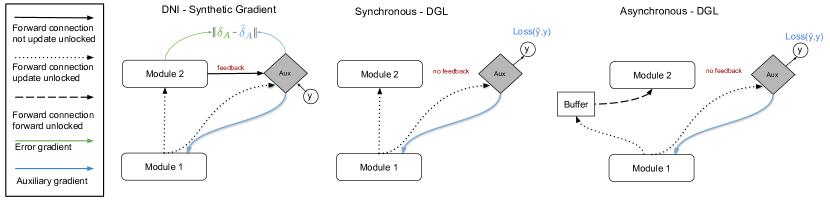
Figure 1: Comparison of DNI, Synchronous and Asynchronous DGL. Note that in DGL subsequent modules do not provide feedback to earlier modules, thus removing dependencies of the auxiliary network on backpropagated gradient information. Asynchronous DGL allows achieving forward unlocking (updates can be performed without waiting for prior modules).

1 Introduction

Jointly training all layers using back-propagation and stochastic optimization is the standard method for learning neural networks, including the computationally intensive Convolutional Neural Networks (CNNs). Due to the sequential nature of gradient processing, standard back-propagation has several well-known inefficiencies that prohibit parallelization of the computations of the different constituent modules. Jaderberg et al. (2017) characterize these inefficiencies in order of severity as the forward-, update-, and backward locking problems. Backward unlocking of a module would permit updates of all modules once forward signals have propagated to all subsequent modules, update unlocking would permit updates of a module before a signal has reached all subsequent modules, and forward unlocking would permit a module to operate asynchronously from its predecessor and dependent modules.

Methods addressing backward locking to a certain degree have been proposed in (Huo et al., 2018b, a; Choromanska et al., 2018; Nø kland, 2016). However, update locking is a far more severe inefficiency. Thus Jaderberg et al. (2017) and Czarnecki et al. (2017) propose and analyze Decoupled Neural Interfaces (DNI), a method that uses an auxiliary network to predict the gradient of the backward pass directly from the input. This method unfortunately does not scale well computationally or in terms of accuracy, especially in the case of CNNs (Huo et al., 2018a, b). Indeed, auxiliary networks must predict a weight gradient, usually high-dimensional for larger models and input sizes.

A major obstacle to update unlocking is the heavy reliance on the upper modules for feedback. Several works have recently revisited the classic (Ivakhnenko and Lapa, 1965; Bengio et al., 2007) approach of supervised greedy layerwise training of neural networks (Huang et al., 2018a; Marquez et al., 2018). In Belilovsky et al. (2019) it is shown that such an approach, which relaxes the joint learning objective, and does not require global feedback, can lead to high-performance deep CNNs on large-scale datasets. We will show that the greedy sequential learning objective used in these papers can be efficiently solved with an alternative parallel optimization algorithm, which permits decoupling the computations and achieves update unlocking. This then opens the door to extend to a forward unlocked model, which is a challenge not effectively addressed by any of the prior work. In particular, we use replay buffers (Lin, 1992) to achieve forward unlocking. This simple strategy can be shown to be a superior baseline for parallelizing the training across modules of a neural network. A training procedure that permits forward and update unlocked computation allows for model components to communicate infrequently and be trained in low-bandwidth settings such as across geographically distant nodes.

The present paper is an extended version of (Belilovsky et al., 2020) that expands the asynchronous (forward unlocked) algorithm, addressing some of its key limitations. In particular, a major issue of replay buffers used to store intermediate representations is that they can grow large, requiring large amounts of on-node memory and more critically increasing inter-node bandwidth. We introduce and evaluate a potential path for drastically reducing the bandwidth constraints between nodes in the case of asynchronous DGL as well as reducing the need for on-node memory. In order to address this issue, a natural approach is compression. However, the replay buffers here store time-varying activations. In this context and inspired by Caccia et al. (2020); Oord et al. (2017) we thus propose a computationally efficient method for online learned compression using codebooks. Specifically, we introduce in Sec. 2.4 and test in Sec. 4.4, the use of a quantization module that compresses the intermediary features used between successive layers but is able to rapidly adapt to distribution shifts. In complement to Belilovsky et al. (2020), this module can deal with online distributions and regularly update a code-book that memorizes some attributes of the current stream of data. It allows to both reduce significantly the local memory of a node as well as the transmission between two subsequent machines, without significantly decreasing the final accuracy of our models. We further show that for a fixed budget of memory, this new method outperforms the algorithm introduced in Belilovsky et al. (2020).

The paper is structured as follows. In Sec. 2 we propose an optimization procedure for a decoupled greedy learning objective that achieves update unlocking and then extend it to an asynchronous setting (async-DGL) using a replay buffer, addressing forward unlocking. Further, we introduce a new quantization module that reduces the memory use of our method. In Sec. 3 we show that the proposed optimization procedure converges and recovers standard rates of non-convex optimization, motivating empirical observations in the subsequent experimental section. In Sec. 4 we show that DGL can outperform competing methods in terms of scalability to larger and deeper models and stability to optimization hyperparameters and overall parallelism, allowing it to be applied to large datasets such as ImageNet. In Sec. 4.4, we test our new quantization module on CIFAR-10. We extensively study async-DGL and find that it is robust to significant delays. In several experiments we show that buffer quantization improves both performance and memory consumption. We also empirically study the impact of parallelized training on convergence. Code for experiments is included in the submission.

2 Parallel Decoupled Greedy Learning

In this section we formally define the greedy objective and parallel optimization which we study in both the synchronous and asynchronous setting. We mainly consider the online setting and assume a stream of samples or mini-batches denoted $\mathcal{S}\triangleq\{(x_{0}^{t},y^{t})\}_{t\leq T}$, run during $T$ iterations.

2.1 Preliminaries

For comparison purposes, we briefly review the update unlocking approach from DNI (Jaderberg et al., 2017). There, each network module has an associated auxiliary net which, given the output activation of the module, predicts the gradient signal from subsequent modules: the module can thus perform an update while modules above are still forward processing. The DNI auxiliary model is trained by using true gradients provided by upper modules when they become available, requiring activation caching. This also means that the auxiliary module can become out of sync with the changing output activation distribution, often requiring slow learning rates. Due to this and the high dimensionality of the predicted gradient which scales with module size, this estimate is challenging. One may ask how well a method that entirely avoids the use of feedback from upper modules would fare given similarly-sized auxiliary networks. We will show that adapting the objective in (Belilovsky et al., 2019; Bengio et al., 2007) can also allow for update unlock and a degree of forward unlocking, with better properties.

Input: Stream $\mathcal{S}\triangleq\{(x_{0}^{t},y^{t})\}_{t\leq T}$ of samples or mini-batches.

1 Initialize Parameters $\{\theta_{j},\gamma_{j}\}_{j\leq J}$.

2 for  $(x_{0}^{t},y^{t})\in\mathcal{S}$  do

3       for $j\in 1,...,J$ do

4            $x^{t}_{j}\leftarrow f_{\theta_{j-1}}(x^{t}_{j-1})$.

5             Compute $\nabla_{(\gamma_{j},\theta_{j})}\hat{\mathcal{L}}(y^{t},x^{t}_{j};\gamma_{j},\theta_{j})$.

6             $(\theta_{j},\gamma_{j})\leftarrow$Update parameters $(\theta_{j},\gamma_{j})$.

7       end for

8      

9 end for

Algorithm 1 Synchronous DGL

Input: Stream $\mathcal{S}\triangleq\{(x_{0}^{t},y^{t})\}_{t\leq T}$; Distribution of the delay $p=\{p(j)\}_{j}$; Buffer size $M$.

1 Initialize: Buffers $\{B_{j}\}_{j}$; params $\{\theta_{j},\gamma_{j}\}_{j}$.

2 while  training do

3      Sample $j$ in $\{1,...,J\}$ following $p$.

4       if $j=1$ then

5             $(x_{0},y)\leftarrow\mathcal{S}$

6      else

7             $(x_{j-1},y)\leftarrow B_{j-1}$.

8       end if

9      $x_{j}\leftarrow f_{\theta_{j-1}}(x_{j-1})$.

10       Compute $\nabla_{(\gamma_{j},\theta_{j})}\hat{\mathcal{L}}(y,x_{j};\gamma_{j},\theta_{j})$.

11       $(\theta_{j},\gamma_{j})\leftarrow$ Update parameters $(\theta_{j},\gamma_{j})$.

12       if $j<J$ then  $B_{j}\leftarrow(x^{j},y)$.

13      

14 end while

Algorithm 2 Asynchronous DGL with Replay

Input: Stream $\mathcal{S}\triangleq\{(x_{0}^{t},y^{t})\}_{t\leq T}$; Distribution of the delay $p=\{p(j)\}_{j}$; Buffer size $M$. Codebooks $\{\mathcal{C}_{j}\}_{j}$. Codebook update delay $T_{code}$

1 Initialize: Buffers $\{B_{j}\}_{j}$; params $\{\theta_{j},\gamma_{j}\}_{j}$; codebooks $\{\mathcal{C_{j}}\}_{j}$.

2 while  training do

3      Sample $j$ in $\{1,...,J\}$ following $p$.

4       if $j=1$ then

5             $(x_{0},y)\leftarrow\mathcal{S}$

6      else

7             $(\tilde{x}_{j-1},y)\leftarrow B_{j-1}$.

8             $x_{j-1}=\text{UnQuantize}(\tilde{x}_{j-1},\mathcal{C}_{j})$

9       end if

10      $x_{j}\leftarrow f_{\theta_{j-1}}(x_{j-1})$.

11       Compute $\nabla_{(\gamma_{j},\theta_{j})}\hat{\mathcal{L}}(y,x_{j};\gamma_{j},\theta_{j})$.

12       $(\theta_{j},\gamma_{j})\leftarrow$ Update parameters $(\theta_{j},\gamma_{j})$.

13       If $j\%T_{code}$: ReceiveCodebooks $\{\mathcal{C}_{j}\}$.

14       if $j<J$ then  $B_{j}\leftarrow(\text{Quantize}[x^{j}],y)$.

15      

16 end while

17

Algorithm 3 Asynchronous DGL with Replay and Quantized modules

2.2 Optimization for Greedy Objective

Let $\bm{X}_{0}$ and $Y$ be the data and labels, $\bm{X_{j}}$ be the output representation for module $j$. We will denote the per-module objective function $\hat{\mathcal{L}}(\bm{X}_{j},Y;\theta_{j},\gamma_{j})$, where the parameters $\theta_{j}$ correspond to the module parameter (i.e. $\bm{X}_{j+1}=f_{\theta_{j}}(\bm{X}_{j})$). Here $\gamma_{j}$ represents parameters of the auxiliary networks used to predict the final target and compute the local objective. $\hat{\mathcal{L}}$ in our case will be the empirical risk with a cross-entropy loss. The greedy training objective is thus given recursively by defining $P_{j}$:

$$\min_{\theta_{j},\gamma_{j}}\hat{\mathcal{L}}(\bm{X}_{j},Y;\theta_{j},\gamma_{j}), P_{j}$$ ()

where $\bm{X}_{j}=f_{\theta_{j-1}^{*}}(\bm{X}_{j-1})$ and $\theta_{j-1}^{*}$ is the minimizer of Problem ($P_{j-1}$). A natural way to solve the optimization problem for $J$ modules, $(P_{J})$, is thus by sequentially solving the problems $\{P_{j}\}_{j\leq J}$ starting with $j=1$. This is the approach taken in e.g. Marquez et al. (2018); Huang et al. (2018a); Bengio et al. (2007); Belilovsky et al. (2019). Here we consider an alternative procedure for optimizing the same objective, which we refer to as Sync-DGL. It is outlined in Alg 1. In Sync-DGL individual updates of each set of parameters are performed in parallel across the different layers. Each layer processes a sample or mini-batch, then passes it to the next layer, while simultaneously performing an update based on its own local loss. Note that at line $5$ the subsequent layer can already begin computing line $4$. Therefore, this algorithm achieves update unlocking. Once $x_{j}^{t}$ has been computed, subsequent layers can begin processing. Sync-DGL can also be seen as a generalization of the biologically plausible learning method proposed in concurrent work (Nøkland and Eidnes, 2019). Appendix D also gives an explicit version of an equivalent multi-worker pseudo-code. Fig. 1 illustrates the decoupling compared to how samples are processed in the DNI algorithm.

In this work we solve the sub-problems $P_{j}$ by backpropagation, but we note that any iterative solver available for $P_{j}$ will be applicable (e.g. Choromanska et al. (2018)). Finally we emphasize that unlike the sequential solvers of (e.g. Bengio et al. (2007); Belilovsky et al. (2019)) the distribution of inputs to each sub-problem solver changes over time, resulting in a learning dynamic whose properties have never been studied nor contrasted with sequential solvers.

2.3 Asynchronous DGL with Replay

We can now extend this framework to address forward unlocking (Jaderberg et al., 2017). DGL modules already do not depend on their successors for updates. We can further reduce dependency on the previous modules such that they can operate asynchronously. This is achieved via a replay buffer that is shared between adjacent modules, enabling them to reuse older samples. Scenarios with communication delays or substantial variations in speed between layers/modules benefit from this. We study one instance of such an algorithm that uses a replay buffer of size $M$, shown in Alg. 2 and illustrated in Fig. 1.

Our minimal distributed setting is as follows. Each worker $j$ has a buffer that it writes to and that worker $j+1$ can read from. The buffer uses a simple read/write protocol. A buffer $B_{j}$ lets layer $j$ write new samples. When it reaches capacity it overwrites the oldest sample. Layer $j+1$ requests samples from the buffer $B_{j}$. They are selected by a last-in-first-out (LIFO) rule, with precedence for the least reused samples. Alg. 2 simulates potential delays in such a setup by the use of a probability mass function (pmf) $p(j)$ over workers, analogous to typical asynchronous settings such as (Leblond et al., 2017). At each iteration, a layer is chosen at random according to $p(j)$ to perform a computation. In our experiments we limit ourselves to pmfs that are uniform over workers except for a single layer which is chosen to be selected less frequently on average. Even in the case of a uniform pmf, asynchronous behavior will naturally arise, requiring the reuse of samples. Alg. 2 permits a controlled simulation of processing speed discrepancies and will be used over settings of $p$ and $M$ to demonstrate that training and testing accuracy remain robust in practical regimes. Appendix D also provides pseudo-code for implementation in a parallel environment.

Unlike common data-parallel asynchronous algorithms (Zhang et al., 2015), the asynchronous DGL does not rely on a master node and requires only local communication similar to recent decentralized schemes (Lian et al., 2017). Contrary to decentralized SGD, DGL nodes only need to maintain and update the parameters of their local module, permitting much larger modules. Combining asynchronous DGL with distributed synchronous SGD for sub-problem optimization is a promising direction. For example it can alleviate a common issue of the popular distributed synchronous SGD in deep CNNs, which is the often limiting maximum batch size (Goyal et al., 2017).

2.4 Reducing the memory- and communication footprint of Asynchronous DGL

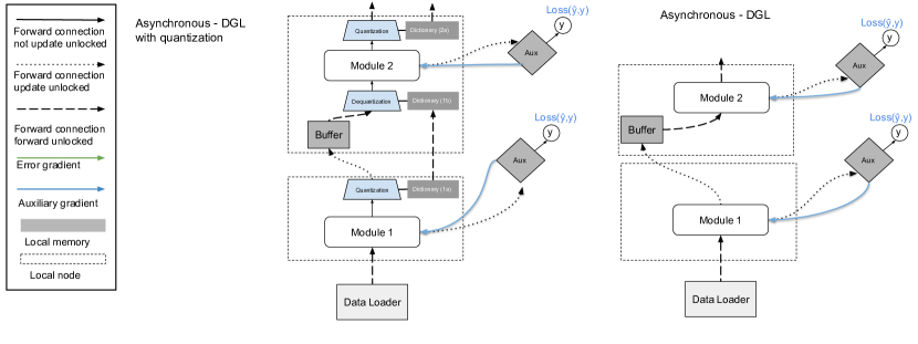
Figure 2: Schematic diagram that explains how the buffers and encoder/decoder quantization modules are incorporated. (left) with quantization (right) without quantization.

The typical objective of an optimization procedure distributed along $H$ nodes is to linearly reduce by $\mathcal{O}(H)$ the training time compared to using a single node. However, in practical applications, the speed-up is in general sub-linear due to communication issues: bandwidth restrictions (e.g., a bandwidth bottleneck or a significant lag between distant nodes) can substantially increase the communication time. In a distributed use case Sync-DGL and Async-DGL would be bottlenecked by communication bandwidth. As the model grows larger, features must be sent across nodes. Similarly for Async DGL the local memory footprint might also be an issue if each node is a device with limited available computational resources. We propose a solution to this problem based on an online dictionary learning algorithm, which is able to rapidly adapt a compression algorithm to the changing features at each node, leading to a large reduction in communication bandwidth and memory. The method is illustrated in Fig. 2 and the algorithm we used is given in Alg. 3.

As illustrated in the Figure 2 we propose to incorporate a quantization module that relies on a codebook with $C$ atoms. Following van den Oord et al. (2017), the quantization step works as follows: each output feature is assigned to its closest atom in its local encoding codebook and the decoding step consists simply in recovering the corresponding atom via its local decoding codebook. The numbers of bits required to encode a single quantized vector is thus $\lceil\log_{2}(C)\rceil$ bits.

During training, the distribution of features at each layer is changing, so the codebooks must be updated online. We must also send the codes to the subsequent node to synchronize the codebooks of two distant communicating modules, so that the following node can decode. Notably the rate at which codebooks are synchronized need not be the same as the rate at which features are sent. We write $\alpha\in[0,1]$ the synchronization rate of the codebooks: We only synchronize the codebook during a selected fraction $\alpha$ of the training iterations. Empirically we will illustrate in the sequel that the codebooks can be synchronized infrequently as compared to the rate a module sends out features. The codebook is updated via an EM algorithm that is learning to minimize the reconstruction error of a given batch of samples, as done in van den Oord et al. (2017); Caccia et al. (2020). In order to deal with batches of data, the dictionary is updated with Exponential Moving Averages (EMA).

We will now discuss the bandwidth and memory savings of the quantization module by deriving explicit equations. First, let us introduce the necessary notations. In the following, at a given module indexed by $j$, we write $\mathcal{B}$ the batch size of a batch $x_{j}$ of features with dimension $K_{j}\times N_{j}^{2}$, where $N_{j}$ corresponds to the spatial size of $x_{j}$ and $K_{j}$ is the number of channels. Assuming the variables are coded as 32-bit floating point numbers, this implies that without quantization, a batch of features will require $32\mathcal{B}N_{j}^{2}K_{j}\,\text{bits}$. Similarly, the buffer memory, which is required in this case, corresponds to $32MN_{j}^{2}K_{j}$, where we always have $M>\mathcal{B}$ in order to avoid sampling issues for sampling a new batch of data.

As in Caccia et al. (2020); van den Oord et al. (2017) we incorporate a spatial structure to our encoding-decoding mechanism: our quantization algorithm will encode the feature vector at each spatial location using the same encoding procedure, leading to a spatial array of codebook indices. Furthermore, as done in Caccia et al. (2020), we assume that we use $k=32$ codebooks to encode respectively each fraction $\lfloor\frac{K_{j}}{k}\rfloor$ of the channel of a given batch. This implies that the communication between two successive modules will require for a single batch of size $\mathcal{B}$:

$$\mathcal{B}kN_{j}^{2}\lceil\log_{2}(C)\rceil+\alpha 32(K_{j}+K_{j-1})C\,\text{ bits.}$$ (1)

Obtained in a similar fashion, the memory footprint of the buffer will be reduced to:

$$MkN_{j}^{2}\lceil\log_{2}(C)\rceil+32K_{j}C\,\text{ bits}\,.$$ (2)

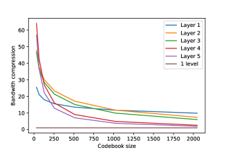
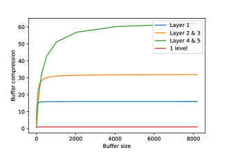
Figure 3: Illustration of bandwidth and buffer memory Compression factors as given by Eq.  (3) and Eq.  (4) for $\alpha=1$ at various depths for a specific CNN model (from Sec. 4.4). On the left figure, we display the bandwidth compression factor as a function of the number of codebook atoms. The right figure corresponds to the buffer compression factor when the buffer size increases. We observe that in all cases we have substantial reduction in bandwidth and memory. Note the buffer size memory compression is variable due to the size of the codebook. For simplicity, we employed the architecture of Sec. 4.3.

As a consequence, we can define two different compression factors when implementing the quantization inside the buffer. The bandwidth compression is defined as

$$C_{b}=\frac{32\mathcal{B}N_{j}^{2}K_{j}}{\mathcal{B}kN_{j}^{2}\log_{2}(C)+\alpha 32(K_{j}+K_{j-1})C},$$ (3)

and indicates an improvement when it is greater than 1. The buffer compression is defined as

$$C_{n}=\frac{32MN_{j}^{2}K_{j}}{MkN_{j}^{2}\log_{2}(C)+32K_{j}C},$$ (4)

and indicates an improvement if it is greater than 1.

As an illustration in Fig. 3 displays the bandwidth reduction factor for a reference network, similar to one to be studied in the sequel, as a function of codebook size $C$. Our reference network has $N_{j}\in[32,16,16,8,8]$, $B=128$, $K_{j}\in[128,256,256,512,512]$, and $\alpha=1$, as well as the buffer memory reduction factor as a function of the buffer size $M$ at a constant codebook size of $C=256$. Note that in both cases, the memory footprint used by the codebook is small compared that of the quantized features. The compression at the buffer level increases when the buffer does. It reaches a threshold defined by the ratio of codebook encoding size and uncompressed channel sizes. However the Bandwidth compression decreases, as increasing codebook size becomes more and more similar to working in 32-bit precision.

2.5 Auxiliary and Primary Network Design

Like DNI our procedure relies on an auxiliary network to obtain update signal. Both methods thus require auxiliary network design in addition to the main CNN architecture. Belilovsky et al. (2019) have shown that spatial averaging operations can be used to construct a scalable auxiliary network for the same objective as used in Sec 2.2. However, they did not directly consider the parallel training use case, where additional care must be taken in the design: The primary consideration is the relative speed of the auxiliary network with respect to its associated main network module. We will use primarily FLOP count in our analysis and aim to restrict our auxiliary networks to be $5\%$ of the main network.

Although auxiliary network design might seem like an additional layer of complexity in CNN design and may require invoking slightly different architecture principles, this is not inherently prohibitive since architecture design is often related to training (e.g., the use of residuals is originally motivated by optimization issues inherent to end-to-end backprop (He et al., 2016)).

Finally, we note that although we focus on the distributed learning context, this algorithm and associated theory for greedy objectives is generic and has other potential applications. For example greedy objectives have recently been used in (Haarnoja et al., 2018; Huang et al., 2018a) and even with a single worker DGL reduces memory.

3 Theoretical Analysis

We now study the convergence results of DGL. Since we do not rely on any approximated gradients, we can derive stronger properties than DNI Czarnecki et al. (2017), such as a rate of convergence in our non-convex setting. To do so, we analyze Alg. 1 when the update steps are obtained from stochastic gradient methods. We show convergence guarantees (Bottou et al., 2018) under reasonable assumptions. In standard stochastic optimization schemes, the input distribution fed to a model is fixed (Bottou et al., 2018). In this work, the input distribution to each module is time-varying and dependent on the convergence state of the previous module. At time step $t$, for simplicity we will denote all parameters of a module (including auxiliary) as $\Theta_{j}^{t}\triangleq(\theta_{j}^{t},\gamma_{j}^{t})$, and samples as $Z_{j}^{t}\triangleq(X_{j}^{t},Y^{t})$, which follow the density $p_{j}^{t}(z)$. For each auxiliary problem, we aim to prove the strongest existing guarantees (Bottou et al., 2018; Huo et al., 2018a) for the non-convex setting despite time-varying input distributions from prior modules. Proofs are given in the Appendix.

Let us fix a depth $j$, such that $j>1$ and consider the converged density of the previous layer, $p^{*}_{j-1}(z)$. We consider the total variation distance: $c^{t}_{j-1}\triangleq\int|p_{j-1}^{t}(z)-p_{j-1}^{*}(z)|\,dz$. Denoting $\ell$ the composition of the non-negative loss function and the network, we will study the expected risk $\mathcal{L}(\Theta_{j})\triangleq\mathbb{E}_{p^{*}_{j-1}}[\ell(Z_{j-1};\Theta_{j})]$. We will now state several standard assumptions we use.

Assumption 1 ($L$-smoothness)

$\mathcal{L}$ is differentiable and its gradient is $L$-Lipschitz.

We consider the SGD scheme with learning rate $\{\eta_{t}\}_{t}$:

$$\Theta^{t+1}_{j}=\Theta^{t}_{j}-\eta_{t}\nabla_{\Theta_{j}}\ell(Z_{j-1}^{t};\Theta_{j}^{t}),$$ (5)

where $Z^{t}_{j-1}\sim p_{j-1}^{t}$.

Assumption 2 (Robbins-Monro conditions)

The step sizes satisfy $\sum_{t}\eta_{t}=\infty$ yet $\sum_{t}\eta_{t}^{2}<\infty$.

Assumption 3 (Finite variance)

There exists $G>0$ such that $\forall t,\Theta_{j},\mathbb{E}_{p^{t}_{j-1}}\big{[}\|\nabla_{\Theta_{j}}\ell(Z_{j-1};\Theta_{j})\|^{2}\big{]}\leq G$.

The Assumptions 1, 2 and 3 are standard (Bottou et al., 2018; Huo et al., 2018a), and we show in the following that our proof of convergence leads to similar rates, up to a multiplicative constant. The following assumption is specific to our setting where we consider a time-varying distribution:

Assumption 4 (Convergence of the previous layer)

We assume that $\sum_{t}c^{t}_{j-1}<\infty$.

Lemma 1

Under Assumption 3 and 4, for all $\Theta_{j},$ one has $\mathbb{E}_{p^{*}_{j-1}}\big{[}\|\nabla_{\Theta_{j}}\ell(Z_{j-1};\Theta_{j})\|^{2}\big{]}\leq G$.

We are now ready to prove the core statement for the convergence results in this setting:

Lemma 2

Under Assumptions 1, 3 and 4, we have:

$$\mathbb{E}[\mathcal{L}(\Theta_{j}^{t+1})] \leq \mathbb{E}[\mathcal{L}(\Theta_{j}^{t})]+\frac{LG}{2}\eta_{t}^{2}\,$$

$$-\eta_{t}\big{(}\mathbb{E}[\|\nabla\mathcal{L}(\Theta_{j}^{t})\|^{2}]-G\sqrt{2c^{t}_{j-1}}\big{)}.$$

The expectation is taken over each random variable. Also, note that without the temporal dependency (i.e. $c_{j}^{t}=0$), this becomes analogous to Lemma 4.4 in (Bottou et al., 2018). Naturally it follows, that

Proposition 3

Under Assumptions 1, 2, 3 and 4, each term of the following equation converges:

$$\sum_{t=0}^{T}\eta_{t}\mathbb{E}[\|\nabla\mathcal{L}(\Theta_{j}^{t})\|^{2}] \leq\mathbb{E}[\mathcal{L}(\Theta^{0}_{j})]$$

$$+G\sum_{t=0}^{T}\eta_{t}\left(\sqrt{2c_{j-1}^{t}}+\frac{L\eta_{t}}{2}\right).$$

Thus the DGL scheme converges in the sense of (Bottou et al., 2018; Huo et al., 2018a). We can also obtain the following rate:

Corollary 4

The sequence of expected gradient norm accumulates around 0 at the following rate:

$$\inf_{t\leq T}\mathbb{E}[\|\nabla\mathcal{L}(\Theta_{j}^{t})\|^{2}]\leq\mathcal{O}\left(\frac{\sum_{t=0}^{T}\sqrt{c_{j-1}^{t}}\eta_{t}}{\sum_{t=0}^{T}\eta_{t}}\right)\,.$$ (6)

Thus compared to the sequential case, the parallel setting adds a delay that is controlled by $\sqrt{c_{j-1}^{t}}$.

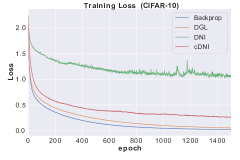
Figure 4: Comparison of DNI, cDNI, and DGL in terms of training loss and test accuracy for experiment from (Jaderberg et al., 2017). DGL converges better than cDNI and DNI with the same auxiliary net. and generalizes better than backprop.

4 Experiments

We conduct experiments that empirically show that DGL optimizes the greedy objective well, showing that it is favorable to recent state-of-the-art proposals for decoupling training of deep network modules. We show that unlike previous decoupled proposals it can still work on a large-scale dataset (ImageNet) and that it can, in some cases, generalize better than standard back-propagation. We then extensively evaluate the asynchronous version of DGL, simulating large delays. For all experiments we use architectures taken from prior works and standard optimization settings.

4.1 Other Approaches and Auxiliary Network Designs

This section presents experiments evaluating DGL with the CIFAR-10 dataset (Krizhevsky, 2009) and standard data augmentation. We first use a setup that permits us to compare against the DNI method and which also highlights the generality and scalability of DGL. We then consider the design of a more efficient auxiliary network which will help to scale to the ImageNet dataset. We will also show that DGL is effective at optimizing the greedy objective compared to a naive sequential algorithm.

Comparison to DNI

We reproduce the CIFAR-10 CNN experiment described in (Jaderberg et al., 2017), Appendix C.1. This experiment utilizes a 3 layer network with auxiliary networks of 2 hidden CNN layers. We compare our reproduction to the DGL approach. Instead of the final synthetic gradient prediction for the DGL we apply a final projection to the target prediction space. Here, we follow the prescribed optimization procedure from (Jaderberg et al., 2017), using Adam with a learning rate of $3\times 10^{-5}$. We run training for 1500 epochs and compare standard backprop, DNI, context DNI (cDNI) (Jaderberg et al., 2017) and DGL. Results are shown in Fig. 4. Details are included in the Appendix. The DGL method outperforms DNI and the cDNI by a substantial amount both in test accuracy and training loss. Also in this setting, DGL can generalize better than standard backprop and obtains a close final training loss.

We also attempted DNI with the more commonly used optimization settings for CNNs (SGD with momentum and step decay), but found that DNI would diverge when larger learning rates were used, although DGL sub-problem optimization worked effectively with common CNN optimization strategies. We also note that the prescribed experiment uses a setting where the scalability of our method is not fully exploited. Each layer of the primary network of (Jaderberg et al., 2017) has a pooling operation, which permits the auxiliary network to be small for synthetic gradient prediction. This however severely restricts the architecture choices in the primary network to using a pooling operation at each layer. In DGL, we can apply the pooling operations in the auxiliary network, thus permitting the auxiliary network to be negligible in cost even for layers without pooling (whereas synthetic gradient predictions often have to be as costly as the base network). Overall, DGL is more scalable, accurate and robust to changes in optimization hyper-parameters than DNI.

Auxiliary Network Design

We consider different auxiliary networks for CNNs. As a baseline we use convolutional auxiliary layers as in (Jaderberg et al., 2017) and (Belilovsky et al., 2019). For distributed training application this approach is sub-optimal as the auxiliary network can be substantial in size compared to the base network, leading to poorer parallelization gains. We note however that even in those cases (that we don’t study here) where the auxiliary network computation is potentially on the order of the primary network, it can still give advantages for parallelization for very deep networks and many available workers.

The primary network architecture we use for this study is a simple CNN similar to VGG family of models (Simonyan and Zisserman, 2014) and those used in (Belilovsky et al., 2019). It consists of 6 convolutions of size $3\times 3$, batchnorm and shape preserving padding, with $2\times 2$ maxpooling at layers 1 and 3. The width of the first layer is 128 and is doubled at each downsampling operation. The final layer does not have an auxiliary model– it is followed by a pooling and 2-hidden layer fully connected network, for all experiments. Two alternatives to the CNN auxiliary of (Belilovsky et al., 2019) are explored (Tab. 1).

	Relative FLOPS	Acc.
CNN-aux	$200\%$	92.2
MLP-aux	$0.7\%$	90.6
MLP-SR-aux	$4.0\%$	91.2

Table 1: Comparison of auxiliary networks on CIFAR. CNN-aux applied in previous work is inefficient w.r.t. the primary module. We report flop count of the aux net relative to the largest module. MLP-aux and MLP-SR-aux applied after spatial averaging operations are far more effective with min. acc. loss.

The baseline auxiliary strategy based on (Belilovsky et al., 2019) and (Jaderberg et al., 2017) applies 2 CNN layers followed by a $2\times 2$ averaging and projection, denoted as CNN-aux. First, we explore a direct application of the spatial averaging to $2\times 2$ output shape (regardless of the resolution) followed by a 3-layer MLP (of constant width). This is denoted MLP-aux and drastically reduces the FLOP count with minimal accuracy loss compared to CNN-aux. Finally, we study a staged spatial resolution, first reducing the spatial resolution by 4$\times$ (and total size 16$\times$), then applying 3 $1\times 1$ convolutions followed by a reduction to $2\times 2$ and a 3 layer MLP, that we denote as MLP-SR-aux. These latter two strategies that leverage the spatial averaging produce auxiliary networks that are less than $5\%$ of the FLOP count of the primary network even for large spatial resolutions as in real world image datasets. We will show that MLP-SR-aux is still effective even for the large-scale ImageNet dataset. We note that these more effective auxiliary models are not easily applicable in the case of DNI’s gradient prediction.

Sequential vs. Parallel Optimization of Greedy Objective

We briefly compare the sequential optimization of the greedy objective (Belilovsky et al., 2019; Bengio et al., 2007) to the DGL (Alg. 1). We use a 6 layer CIFAR-10 network with an MLP-SR-aux auxiliary model. In parallel we train the layers together for 50 epochs and in the sequential training we train each layer for 50 epochs before moving to the subsequent one. Thus the difference to DGL lies only in the input received at each layer (fully converged previous layer versus not fully converged previous layer). The rest of the optimization settings are identical. Fig. 5 shows comparisons of the learning curves for sequential training and DGL at layer 4 (layer 1 is the same for both as the input representation is not varying over the training period). DGL quickly catches up with the sequential training scheme and appears to sometimes generalize better. Like Oyallon (2017), we also visualize the dynamics of training per layer in Fig. 6, which demonstrates that after just a few epochs the individual layers build a dynamic of progressive improvement with depth.

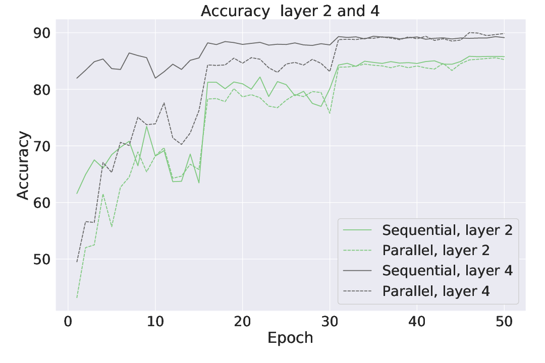
Figure 5: Comparison of sequential and parallel training. Parallel catches up rapidly to sequential.

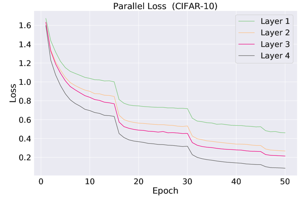
Figure 6: Per layer-loss on CIFAR: after few epochs, the layers build a dynamic of progressive improvement in depth.

Multi-Layer modules

We have so far mainly considered the setting of layer-wise decoupling. This approach however can easily be applied to generic modules. Indeed, approaches such as DNI (Jaderberg et al., 2017) often consider decoupling entire multi-layer modules. Furthermore the propositions for backward unlocking (Huo et al., 2018b, a) also rely on and report they can often only decouple 100 layer networks into 2 or 4 blocks before observing optimization issues or performance losses and require that the number of parallel modules be much lower than the network depth for the theoretical guarantees to hold. As in those cases, using multi-layer decoupled modules can improve performance and is natural in the case of deeper networks. We now use such a multi-layer approach to directly compare to the backward unlocking of (Huo et al., 2018b) and then subsequently we will apply this on deep networks for ImageNet. From here on we will denote $K$ the number of total modules a network is split into.

Comparison to DDG

Huo et al. (2018b) propose a solution to the backward locking (less efficient than solving update-locking, see discussion in Sec 5).

Backprop	DDG	DGL
93.53	93.41	$93.5\pm 0.1$

Table 2: ResNet-110($K=2$) for Backprop and DDG method from (Huo et al., 2018b). DGL is run for 3 trials to compute variance. They give the same acc. with DGL being update unlocked, DDG only backward unlocked. DNI is reported to not work in this setting (Huo et al., 2018b).

We show that even in this situation the DGL method can provide a strong baseline for work on backward unlocking. We take the experimental setup from (Huo et al., 2018b), which considers a ResNet-110 parallelized into $K=2$ blocks. We use the auxiliary network MLP-SR-aux which has less than $0.1\%$ the FLOP count of the primary network. We use the exact optimization and network split points as in (Huo et al., 2018b).

To assess variance in CIFAR-10 accuracy, we perform 3 trials. Tab. 2 shows that the accuracy is the same across the DDG method, backprop, and our approach. DGL achieves better parallelization because it is update unlocked. We use the parallel implementation provided by (Huo et al., 2018b) to obtain a direct wall clock time comparison. We note that there are multiple considerations for comparing speed across these methods (see Appendix C).

Wall Time Comparison

We compare to the parallel implementation of (Huo et al., 2018b) using the same communication protocols and run on the same hardware. We find for $K=2,4$ GPU gives a $~{}5\%,18\%$ respectively speedup over DDG. With DDG $K=4$ giving approximately $2.3\times$ speedup over standard backprop on same hardware (close to results from (Huo et al., 2018b)).

4.2 Large-scale Experiments

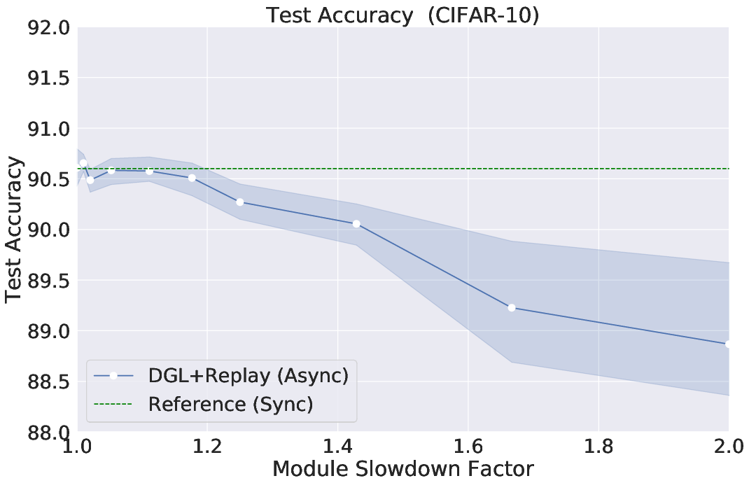
Figure 7: Evaluation of Async DGL. A single layer is slowed down on average over others, with negligible losses of accuracy at even substantial delays.

Model (training method)	Top-1	Top-5
VGG-13 (DGL per Layer, $K=10$)	64.4	85.8
VGG-13 (DGL $K=4$)	67.8	88.0
VGG-13 (backprop)	66.6	87.5
VGG-19 (DGL $K=4$)	69.2	89.0
VGG-19 (DGL $K=2$)	70.8	90.2
VGG-19 (backprop)	69.7	89.7
ResNet-152 (DGL $K=2$)	74.5	92.0
ResNet-152 (backprop)	74.4	92.1

Figure 8: ImageNet results using training schedule of (Xiao et al., 2019) for DGL and standard e2e backprop. DGL with VGG and ResNet obtains similar or better accuracies, while enabling parallelization and reduced memory.

Existing methods considering update or backward locking have not been evaluated on large image datasets as they are often unstable or already show large losses in accuracy on smaller datasets. Here we study the optimization of several well-known architectures, mainly the VGG family (Simonyan and Zisserman, 2014) and the ResNet (He et al., 2016), with DGL on the ImageNet dataset. In all our experiments we use the MLP-SR-aux auxiliary net which scales well from the smaller CIFAR-10 to the larger ImageNet. The final module has no auxiliary network. For all optimization of auxiliary problems and for end-to-end optimization of reference models we use the shortened optimization schedule prescribed in (Xiao et al., 2019). Results are shown in Tab. 8. We see that for all the models DGL can perform as well and sometimes better than the end-to-end trained models, while permitting parallel training. In all these cases the auxiliary networks are neglibile (see Appendix Table 4 for more details). For the VGG-13 architecture we also evaluate the case where the model is trained layer by layer ($K=10$). Although here performance is slightly degraded, we find it is suprisingly high given that no backward communication is performed. We conjecture that improved auxiliary models and combinations with methods such as (Huo et al., 2018a) to allow feedback on top of the local model, may further improve performance. Also for the settings with larger potential parallelization, slower but more performant auxiliary models could potentially be considered as well.

The synchronous DGL has also favorable memory usage compared to DDG and to the DNI method, DNI requiring to store larger activations and DDG having high memory compared to the base network even for few splits (Huo et al., 2018a). Although not our focus, the single worker version of DGL has favorable memory usage compared to standard backprop training. For example, the ResNet-152 DGL $K=2$ setting can fit $38\%$ more samples on a single 16GB GPU than the standard end-to-end training.

4.3 Asynchronous DGL with Replay

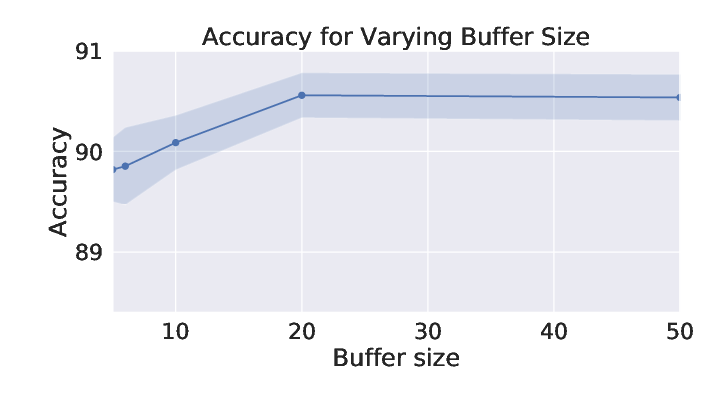
Figure 9: Buffer size vs. Acc. for Async DGL. Smaller buffers produce only small loss in acc.

We now study the effectiveness of Alg. 2 with respect to delays. We use a 5 layer CIFAR-10 network with the MLP-aux and with all other architecture and optimization settings as in the auxiliary network experiments of Sec. 4.1. Each layer is equipped with a buffer of size $M$ samples. At each iteration, a layer is chosen according to the pmf $p(j)$, and a batch selected from buffer $B_{j-1}$. One layer is slowed down by decreasing its selection probability in the pmf $p(j)$ by a factor $S$. We define $S=\frac{p}{p(j)}$, where $p$ is the constant probability of any other worker being selected, so $p=(1-p(j))/(J-1)$. Taken together his implies that:

$$S=\frac{1}{J-1}\left(\frac{1}{p(j)}-1\right)$$ (7)

We evaluate different slowdown factors (up to $S=2.0$). Accuracy versus $S$ is shown in Fig. 8. For this experiment we use a buffer of size $M=50$ samples. We run separate experiments with the slowdown applied at each of the 6 layers of the network as well as 3 random seeds for each of these settings (thus 18 experiments per data point). We show the evaluations for 10 values of $S$. To ensure a fair comparison we stop updating layers once they have completed 50 epochs, ensuring an identical number of gradient updates for all layers in all experiments.

In practice one could continue updating until all layers are trained. In Fig. 8 we compare to the synchronous case. First, observe that the accuracy of the synchronous algorithm is maintained in the setting where $S=1.0$ and the pmf is uniform. Note that even this is a non-trivial case, as it will mean that layers inherently have random delays (as compared to Alg.  1). Secondly, observe that accuracy is maintained until approximately $1.2\times$ and accuracy losses after that the difference remains small. Note that even case $S=2.0$ is somewhat drastic: for 50 epochs, the slowed-down layer is only on epoch 25 while those following it are at epoch 50.

We now consider the performance with respect to the buffer size. Results are shown in Fig. 9. For this experiment we set $S=1.2\times$. Observe that even a tiny buffer size can yield only a slight loss in accuracy. Building on this demonstration there are multiple directions to improve Async DGL with replay. For example improving the efficiency of the buffer Oyallon et al. (2018), by including data augmentation in feature space (Verma et al., 2018), mixing samples in batches, or improved batch sampling, among others.

4.4 Adaptive Online Compression for Async-DGL with Replay

We now evaluate the online compression proposed in Sec. 2.4. We consider the setting of the previous Sec. 4.3. In the subsequent experiments on CIFAR-10 we will consider the same simplified CNN architecture, however to simplify the analysis we will focus on just a 4 module version of this model which will allow us to explore in more depth the behavior of the proposed approach.

Similarly to the previous section on Aync-DGL, we slow down the communication between selected layers. This permits to consider a scenario where each layer is hosted on a different node. In such a setting the communication bandwidth would naturally be bounded. We follow the same training strategy as above: Each layer is asynchronously optimized using SGD with an initial learning rate of 0.1 (with a decay factor of $0.2$ every 15 epochs), momentum of 0.9, a weight decay equal to $5\times 10^{-4}$, and a cross-entropy loss.After completing the equivalent of 50 epochs each layer stops performing updates and only passes signals to upper layers. As in the previous section we use a LIFO priority rule with a penalty for reuse. In all our experiments, results are reported as an averaging over 5 seeds.

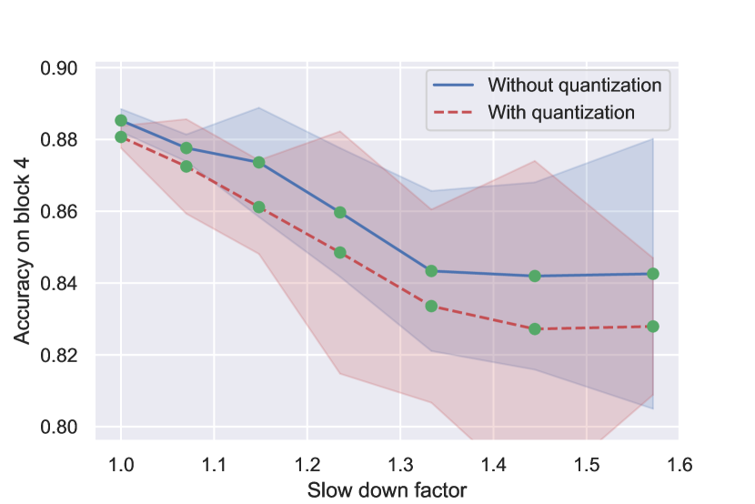
(a) Communication lag between layer 1-2

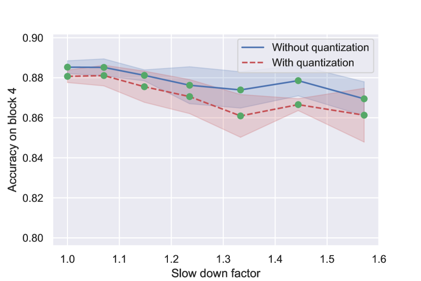
(b) Communication lag between layer 2-3

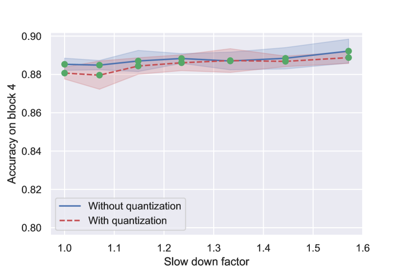
(c) Communication lag between layer 3-4

Figure 10: Comparison between quantization and no quantization: Accuracy when the communication between nodes $i,i+1$ is slowed down for the layers $i=1,2,3$. Using quantization we observe a drop in performance when the slow-down is applied on early layers, but we also note that the slow-down has positive impact when applied to the layer 3. This is expected: layer slow-downs will affect the distribution of the subsequent layers, except if applied to the final layer which can then learn on top of almost converged features.

We follow the adaptive quantization procedure proposed in Sec. 2.4 that encodes and decodes a modules local memory with a learned set of codebooks. With respect to this buffered memory and quantization procedure all experiments are conducted with a buffer of size $M=2$ batches (note the batch size is 128). The number of codebooks with 256 atoms, and a batch size of 128, unless otherwise stated. In all our experiments, we kept constant the number of different codebooks at 32. Each setting was independently run with 5 random seeds: we report the average accuracy with its corresponding confidence interval at $95\%$ level.

The results in this setting are illustrated in Fig. 10. Here we apply a slow-down factor in the range $[1,1.6]$ to each layer, as defined in (7) and we keep all the other hyper-parameters fixed. We compare the numerical accuracy with and without quantization. Compared to the previous section, we refine our study by reporting the accuracy at every depth instead of averaging the accuracies for each given slow-down factor regardless of the position at which it was applied.

Note that, thanks to the quantization module, the communication bandwidth is reduced by a factor $15.5,23.3,21.3$ respectively, and the buffer memory is reduced with a factor in $15.8,28.4,28.4$ respectively. We observe there are small, but potentially acceptable, accuracy losses with quantization depending on where the delay is induced. If it is in the first 2 layers the difference is typically less than $1.5\%$. This improves in cases where the delay is induced at a layer. We hypothesize the 3rd module shows less performance gains when slowed down as it receives features from the previous layers which are potentially changing less dramatically and are more stable. We note that even a $1.5\%$ accuracy loss can be compensated by ability to train much larger models due to parallelization thereby leading to potentially higher accuracy models overall. The results suggest that our Quantized Async-DGL is robust to the distribution shifts incurred by the lag. We now ablate various aspects of the Quantized Async DGL.

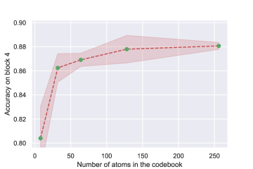
Figure 11: Accuracy at the final layer of our model as a function of the number of atoms. Only 7 bits are necessary to obtain our top accuracies.

Codebook size

We study the impact of the codebook size on the accuracy of a quantized buffer. As expected, the number of atoms in the compression codebook is correlated with performance for small codebook sizes and it reaches a plateau when the number of atoms is large enough. Indeed, the more items in our dictionary, the better is the approximation of the quantization. This means that for a large number of atoms, the accuracy behaves similarly to the non-compressed version, whereas with a small number of atoms, the accuracy depends on the compression rate. For these experiments, no nodes are artificially slowed down. Our results in Fig. 11 illustrate the robustness of our approach. Indeed 128 or 256 atoms are enough to reach standard performances (256 atoms can be encoded using 8 bits, which is to be compared with the 32 bits single floating point precision). The bandwidth compression rate depends on the layer, but is always above 12 in this experiment. Despite this compression, we can still recover accuracies at the level of those obtained in Sec. 5.

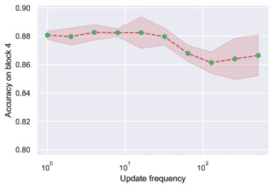
Figure 12: Accuracy of the final block as a function of codebook update frequency. Updating the atoms only one out of 16 iterations still preserves the final accuracy with almost no degradation, while leading to substantial bandwidth saving. In fact, updating the codebook only once every 400 iterations leads to a drop of only $2\%$. This is surprising and indicates that the codebook can be largely ignored when measuring the bandwidth needed for this method

Update Frequency

The codebook size has to be added to the bandwidth use, because a step of synchronization is required as the distribution of the activations is changing with time. Our hypothesis is that the distribution of the features will evolve slowly, making it unnecessary to sync codebooks at every iteration. We choose an update frequency $\alpha\leq 1$, (c.f. Sec. 2.4) and update the codebook only at a fraction $\alpha$ of the iterations. This makes the communications of the dictionary negligible and the procedure may only have minor impact on the final accuracy of our model. We thus propose to study this effect: we only update the weights of the codebook every $\frac{1}{\alpha}>1$ iterations. Fig. 12 shows that the accuracy of our model is extremely stableeven at low update frequency. We note that updating the codebook every 10 iterations preserves the accuracy of the final layer. Then the accuracy drops only by $2\%$ even if the dictionaries of the quantization modules are updated only once per epoch. The final point on our logarithmic scale corresponds to a setting where the codebook is not updated at all: in this particular case, the codebook is randomly initialized, and the network adapts to it. This shows the strength of our method.

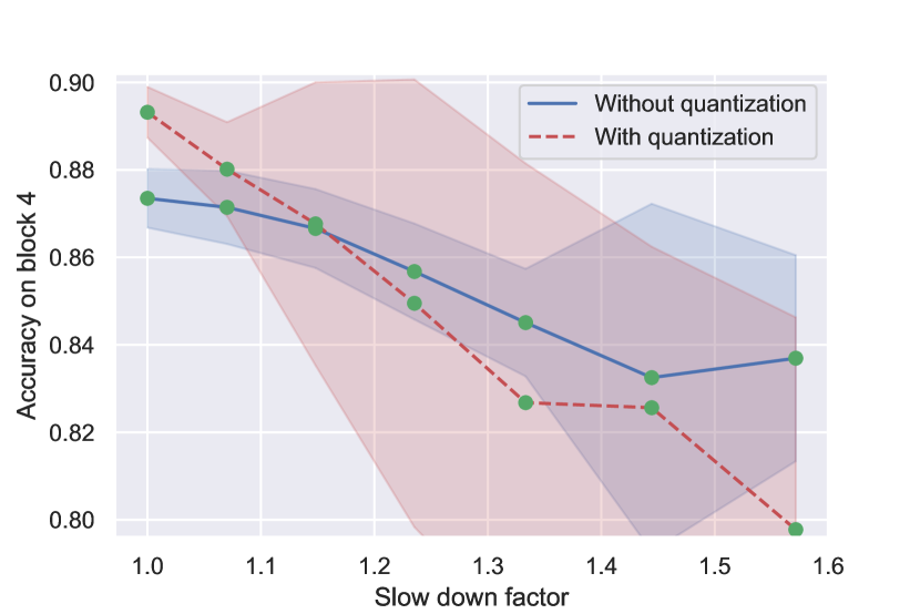
(a) Communication lag between layer 1-2

(b) Communication lag between layer 2-3

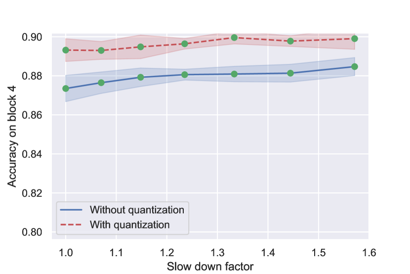
(c) Communication lag between layer 3-4

Figure 13: We compare the test accuracy obtained for our Asynchronous method when we slow down a layer at various depths, with and without a quantization module at a fixed memory budget. We used the hyper-parameters obtained from the Sec. 4.4 and we adjusted the size of the codebook such that the buffer memory used both with and without a quantization step is the same. Interestingly, in every settings, the algorithm which uses quantization outperforms the non-quantized version. Note, if the layer is very out of sync, there is a substantial degradation of the accuracy. Note that slowing down the final layer as in (c) slightly boost the accuracy because this layer is fed with converged features during its last steps of training.

Tradeoff between compression and buffer size at fixed memory budget

In this experiment, we design a setting where each node has the same amount of limited total memory to store both the input and output dictionaries and the the buffer. We then compare at fixed budget the difference between quantized and standard approaches in terms of accuracy. For the non-quantized version, the buffer size is set at 128. For the quantized version, we increase the buffer size until its memory use matches the non-quantized versions. Overall the quantized version can store $[1984~{},~{}3277~{},~{}3277~{},~{}2726]$ samples at layer 1 to 4 respectively. The accuracy is compared between these in Figure 13. We observe the same trend in terms of impact of delays on the accuracy as in Fig. 10. More importantly we observe for a similar Buffer memory consumption that the quantized version reaches better performances than the non-quantized one in almost all cases, which implies that our quantization modules help improve the accuracy at a fixed memory budget. In addition, we also have a (highly) favorable bandwidth compression factor (above 15). As a consequence, for the same Buffer Memory budget, and a weaker bandwidth, the quantized version delivers better performances with and without slow-downs (almost everywhere).

5 Related work

To the best of our knowledge (Jaderberg et al., 2017) is the the first to directly consider the update or forward locking problems in deep feed-forward networks. Other works (Huo et al., 2018a, b) study the backward locking problem. Furthermore, a number of backpropagation alternatives (Choromanska et al., 2018; Lee et al., 2014; Nø kland, 2016) can address backward locking. However, update locking is a more severe inefficiency. Consider the case where each layer’s forward processing time is $T_{F}$ and is equal across a network of $L$ layers. Given that the backward pass is a constant multiple in time of the forward, in the most ideal case the backward unlocking will still only scale as $\mathcal{O}(LT_{F})$ with $L$ parallel nodes, while update unlocking could scale as $\mathcal{O}(T_{F})$.

One class of alternatives to standard back-propagation aims to avoid its biologically implausible aspects, most notably the weight transport problem (Bartunov et al., 2018; Nø kland, 2016; Lillicrap et al., 2014; Lee et al., 2014; Ororbia et al., 2018; Ororbia and Mali, 2019). Some of these methods (Lee et al., 2014; Nø kland, 2016) can also achieve backward unlocking as they permit all parameters to be updated at the same time, but only once the signal has propagated to the top layer. However, they do not solve the update or forward locking problems. Target propagation uses a local auxiliary network as in our approach, for propagating backward optimal activations computed from the layer above. Feedback alignment replaces the symmetric weights of the backward pass with random weights. Direct feedback alignment extends the idea of feedback alignment passing errors from the top to all layers, potentially enabling simultaneous updates. These approaches have also not been shown to scale to large datasets (Bartunov et al., 2018), obtaining only $17.5\%$ top-5 accuracy on ImageNet (reference model achieving $59.8\%$). On the other hand, greedy learning has been shown to work well on this task (Belilovsky et al., 2019). We also note concurrent work in the context of biologically plausible models by (Nøkland and Eidnes, 2019) which improves on results from Mostafa et al. (2018), showing an approach similar to a specific instantiation of the synchronous version of DGL. This work however does not consider the applications to unlocking nor asynchronous training and cannot currently scale to ImageNet.

Another line of related work inspired by optimization methods such as Alternating Direction Method of Multipliers (ADMM) (Taylor et al., 2016; Carreira-Perpinan and Wang, 2014; Choromanska et al., 2018) use auxiliary variables to break the optimization into sub-problems. These approaches are fundamentally different from ours as they optimize for the joint training objective, the auxiliary variables providing a link between a layer and its successive layers, whereas we consider a different objective where a layer has no dependence on its successors. None of these methods can achieve update or forward unlocking. However, some (Choromanska et al., 2018) are able to have simultaneous weight updates (backward unlocked). Another issue with ADMM methods is that most of the existing approaches except for (Choromanska et al., 2018) require standard (“batch”) gradient descent and are thus difficult to scale. They also often involve an inner minimization problem and have thus not been demonstrated to work on large-scale datasets. Furthermore, none of these have been combined with CNNs.

Distributed optimization based on data parallelism is a popular area in machine learning beyond deep learning models and often studied in the convex setting (Leblond et al., 2018). For deep network optimization the predominant method is distributed synchronous SGD (Goyal et al., 2017) and variants, as well as asynchronous (Zhang et al., 2015) variants. Our work is closer to a form of model parallelism rather than data parallelism, and can be easily combined with many data parallel methods (e.g. distributed synchronous SGD). Recently federated learning, where the dataset used on each node is different, has become a popular line of research Konečnỳ et al. (2015). Federated learning is orthogonal to our proposal, but the idea of facilitating different data on each node could potentially be incorporated in our framework. One direction for doing this would consider a class of models where individual layers can provide both input and output to other layers as done in Huang et al. (2016).

Recent proposals for “pipelining” (Huang et al., 2018b) consider systems level approaches to optimize latency times. These methods do not address the update, forward, locking problems(Jaderberg et al., 2017) which are algorithmic constraints of the learning objective and backpropagation. Pipelining can be seen as a attempting to work around these restrictions, with the fundamental limitations remaining. Removing and reducing update, backward, forward locking would simplify the design and efficiency of such systems-level machinery. Tangential to our work Lee et al. (2015) considers auxiliary objectives but with a joint learning objective, which is not capable of addressing any of the problems considered in this work.

We also note that since publication of Belilovsky et al. (2020) several works have extended the methods and studied various things such as how it affects representations Laskin et al. (2020) to allow for improved scalability. However, these works largely consider the synchronous setting and have not extensively considered the asynchronous setting emphasized in Sec. 4.3 and 4.4.

6 Conclusion

We have analyzed and introduced a simple and strong baseline for parallelizing per layer and per module computations in CNN training. This work matches or exceeds state-of-the-art approaches addressing these problems and is able to scale to much larger datasets than others. In several realistic settings, for the same bytes range, an asynchronous framework with quantized buffers can be more robust to delays than a non-quantized version while providing better bandwidth. Future work can develop improved auxiliary problem objectives and combinations with delayed feedback.

Acknowledgements

LL was supported by ANR-20-CHIA-0022-01 ”VISA-DEEP”. EO acknowledges NVIDIA for its GPU donation. EB acknowledges funding from IVADO. This work was granted access to the HPC resources of IDRIS under the allocation 2020-[AD011011216R1] made by GENCI and it was partly supported by ANR-19-CHIA ”SCAI”.

A Proofs

Lemma 1

Under Assumption 3 and 4, one has: $\forall\Theta_{j},\mathbb{E}_{p^{*}_{j-1}}\big{[}\|\nabla_{\Theta_{j}}\ell(Z_{j-1};\Theta_{j})\|^{2}\big{]}\leq G$.

Proof  First of all, observe that under Assumption 4 and via Fubini’s theorem:

$$\sum_{t}c_{j-1}^{t}=\sum_{t}\int|p_{j-1}^{t}(z)-p_{j-1}^{*}(z)|\,dz=\int\sum_{t}|p_{j-1}^{t}(z)-p_{j-1}^{*}(z)|\,dz<\infty$$ (8)

thus, $\sum_{t}|p_{j}^{t}-p_{j}^{*}|$ is convergent a.s. and $|p_{j}^{t}-p_{j}^{*}|\rightarrow 0$ a.s as well. From Fatou’s lemma, one has:

$$\int p^{*}_{j-1}(z)\|\nabla_{\Theta_{j}}\ell(z;\Theta_{j})\|^{2}\,dz =\int\lim\inf_{t}p^{t}_{j-1}(z)\|\nabla_{\Theta_{j}}\ell(z;\Theta_{j})\|^{2}\,dz$$ (9)

$$\leq\lim\inf_{t}\int p^{t}_{j-1}(z)\|\nabla_{\Theta_{j}}\ell(z;\Theta_{j})\|^{2}\,dz\leq G$$ (10)

then, observe that this implies that:

$$p_{j}^{t}(z)\leq p_{j}^{*}(z)+(p_{j}^{t}(z)-p_{j}^{*}(z))\leq p_{j}^{*}(z)+|p_{j}^{t}(z)-p_{j}^{*}(z)|\leq p_{j}^{*}(z)+\sum_{t}|p_{j}^{t}(z)-p_{j}^{*}(z)|$$ (11)

thus, $\sup_{t}p_{j}^{t}$ is integrable because the right term is integrable as well. Then, observe that:

$$\|\nabla\ell_{j,t}\||p^{*}_{j}(z)-p^{t}_{j}(z)|=\|\nabla\ell_{j,t}\|1_{p^{*}_{j}(z)<p^{t}_{j}(z)}|p^{*}_{j}(z)-p^{t}_{j}(z)|+\|\nabla\ell_{j,t}\|1_{p^{*}_{j}(z)\geq p^{t}_{j}(z)}|p^{*}_{j}(z)-p^{t}_{j}(z)|$$

Then, the left term is bounded because:

$$\|\nabla\ell_{j,t}\|1_{p^{*}_{j}(z)<p^{t}_{j}(z)}|p^{*}_{j}(z)-p^{t}_{j}(z)|\leq\|\nabla\ell_{j,t}\|1_{p^{*}_{j}(z)<p^{t}_{j}(z)}p^{t}_{j}(z)\leq\|\nabla\ell_{j,t}\|1_{p^{*}_{j}(z)<p^{t}_{j}(z)}\sup_{t}p^{t}_{j}(z)$$ (12)

$$\int\sum_{t}1_{p^{*}_{j}(z)\geq p^{t}_{j}(z)}(p^{*}_{j}(z)-p^{t}_{j}(z))\,dz\leq\int\sum_{t}1_{p^{*}_{j}(z)=p^{t}_{j}(z)}|p^{*}_{j}(z)-p^{t}_{j}(z)|\,dz<\infty$$

In particular:

$$\int\sum_{t}1_{p^{*}_{j}(z)\geq p^{t}_{j}(z)}p^{*}_{j}(z)\,dz<\infty$$

It implies that $\sum_{t}1_{p^{*}_{j}(z)\geq p^{t}_{j}(z)}$ is almost surely finite, and, a.s. $\forall z,\exists t_{0},p^{*}_{j}(z)\leq p^{t_{0}}_{j}(z)$. In particular this implies that a.s.:

$$\forall z,p^{*}_{j}(z)\leq\sup_{t}p_{j}^{t}(z)$$

 

Lemma 2

Under Assumptions 1, 3 and 4, we have:

$$\mathbb{E}[\mathcal{L}(\Theta_{j}^{t+1})]\leq\mathbb{E}[\mathcal{L}(\Theta_{j}^{t})]-\eta_{t}\big{(}\mathbb{E}[\|\nabla\mathcal{L}(\Theta_{j}^{t})\|^{2}]-\sqrt{2}Gc^{t}_{j-1}\big{)}+\frac{LG}{2}\eta_{t}^{2}\,,$$

Observe that the expectation is taken over each random variable.

Proof  By $L$-smoothness:

$$\mathcal{L}(\Theta_{j}^{t+1})\leq\mathcal{L}(\Theta_{j}^{t}) +\nabla\mathcal{L}(\Theta_{j}^{t})^{T}(\Theta^{t+1}_{j}-\Theta_{j}^{t})+\frac{L}{2}\|\Theta_{j}^{t+1}-\Theta_{j}^{t}\|^{2}$$ (13)

Substituting $\Theta_{j}^{t+1}-\Theta_{j}^{t}$ on the right:

$$\mathcal{L}(\Theta_{j}^{t+1}) \leq\mathcal{L}(\Theta_{j}^{t})-\eta_{t}\nabla\mathcal{L}(\Theta_{j}^{t})^{T}\nabla_{\Theta_{j}}\ell(Z_{j-1}^{t};\Theta_{j}^{t})+\frac{L\eta_{t}^{2}}{2}\|\nabla_{\Theta_{j}}\ell(Z_{j-1}^{t};\Theta_{j}^{t})\|^{2}$$ (14)

Taking the expectation w.r.t. $Z_{j-1}^{t}$ which has a density $p_{j-1}^{t}$, we get:

$$\mathbb{E}_{p^{t}_{j-1}}[\mathcal{L}(\Theta_{j}^{t+1})] \leq\mathcal{L}(\Theta_{j}^{t})-\eta_{t}\nabla\mathcal{L}(\Theta_{j}^{t})^{T}\mathbb{E}_{p_{j-1}^{t}}[\nabla_{\Theta_{j}}\ell(Z_{j-1}^{t};\Theta_{j}^{t})]+\frac{L\eta_{t}^{2}}{2}\mathbb{E}_{p_{j-1}^{t}}\big{[}\|\nabla_{\Theta_{j}}\ell(Z_{j-1}^{t};\Theta_{j}^{t})\|^{2}\big{]}$$

From Assumption 3, we obtain that:

$$\frac{L\eta_{t}^{2}}{2}\mathbb{E}_{p_{j-1}^{t}}\big{[}\|\nabla_{\Theta_{j}}\ell(Z_{j-1}^{t};\Theta_{j}^{t})\|^{2}\big{]}\leq\frac{L\eta_{t}^{2}G}{2}$$ (15)

Then, as a side computation, observe that:

$$\|\mathbb{E}_{p_{j-1}^{t}}\big{[}\nabla_{\Theta_{j}}\ell(Z_{j-1}^{t};\Theta_{j}^{t})\big{]}-\nabla\mathcal{L}(\Theta_{j}^{t})\| =\|\int\nabla\ell(z,\Theta_{j}^{t})p^{t}_{j-1}(z)\,dz-\int\nabla\ell(z,\Theta_{j}^{t})p^{*}_{j-1}(z)\,dz\|$$ (16)

$$\leq\int\|\nabla\ell(z,\Theta_{j}^{t})\|~{}|p^{t}_{j-1}(z)-p^{*}_{j-1}(z)|\,dz$$ (17)

$$=\int\big{(}\|\nabla\ell(z,\Theta_{j}^{t})\|\sqrt{|p^{t}_{j-1}(z)-p^{*}_{j-1}(z)|}\big{)}~{}\sqrt{|p^{t}_{j-1}(z)-p^{*}_{j-1}(z)|}\,dz$$ (18)

Let us apply the Cauchy-Swchartz inequality, we obtain:

$$\|\mathbb{E}_{p_{j-1}^{t}}\big{[}\nabla_{\Theta_{j}}\ell(Z_{j-1}^{t};\Theta_{j}^{t})\big{]}-\nabla\mathcal{L}(\Theta_{j}^{t})\| \leq\sqrt{\int\|\nabla\ell(z,\Theta_{j}^{t})\|^{2}|p^{t}_{j-1}(z)-p^{*}_{j-1}(z)|\,dz}\sqrt{\int|p^{t}_{j-1}(z)-p^{*}_{j-1}(z)|\,dz}$$ (20)

$$=\sqrt{\int\|\nabla\ell(z,\Theta_{j}^{t})\|^{2}|p^{t}_{j-1}(z)-p^{*}_{j-1}(z)|\,dz}\sqrt{c_{j-1}^{t}}$$ (21)

Then, observe that:

$$\int\|\nabla\ell(z,\Theta_{j}^{t})\|^{2}|p^{t}_{j-1}(z)-p^{*}_{j-1}(z)|\,dz \leq\int\|\nabla\ell(z,\Theta_{j}^{t})\|^{2}\big{(}p^{t}_{j-1}(z)+p^{*}_{j-1}(z)\big{)}\,dz$$ (22)

$$=\mathbb{E}_{p^{t}_{j-1}}[\|\nabla\ell(Z_{j-1},\Theta_{j}^{t})\|^{2}]+\mathbb{E}_{p^{*}_{j-1}}[\|\nabla\ell(Z_{j-1},\Theta_{j}^{t})\|^{2}]$$ (23)

$$\leq 2G$$ (24)

The last inequality follows from Lemma 4.1 and Assumption 3.

Then, using again Cauchy-Schwartz inequality:

$$\bigg{|}\|\nabla\mathcal{L}(\Theta_{j}^{t})\|^{2}-\nabla\mathcal{L}(\Theta_{j}^{t})^{T}\mathbb{E}_{p_{j-1}^{t}}[\nabla_{\Theta_{j}}\ell(Z_{j-1}^{t};\Theta_{j}^{t})]\bigg{|} =\bigg{|}\nabla\mathcal{L}(\Theta_{j}^{t})^{T}\big{(}\nabla\mathcal{L}(\Theta_{j}^{t})-\mathbb{E}_{p_{j-1}^{t}}[\nabla_{\Theta_{j}}\ell(Z_{j-1}^{t};\Theta_{j}^{t})]\big{)}\bigg{|}$$ (25)

$$\leq\|\nabla\mathcal{L}(\Theta^{t}_{j})\|~{}\|\mathbb{E}_{p_{j-1}^{t}}\big{[}\nabla_{\Theta_{j}}\ell(Z_{j-1}^{t};\Theta_{j}^{t})\big{]}-\nabla\mathcal{L}(\Theta_{j}^{t})\|$$ (26)

$$\leq\|\nabla\mathcal{L}(\Theta^{t}_{j})\|\sqrt{2Gc^{t}_{j-1}}$$ (27)

Then, taking the expectation leads to

$$\big{|}\mathbb{E}\bigg{[}\|\nabla\mathcal{L}(\Theta_{j}^{t})\|^{2}-\nabla\mathcal{L}(\Theta_{j}^{t})^{T}\mathbb{E}_{p_{j-1}^{t}}[\nabla_{\Theta_{j}}\ell(Z_{j-1}^{t};\Theta_{j}^{t})]\bigg{]}\big{|} \leq\mathbb{E}[\bigg{|}\|\nabla\mathcal{L}(\Theta_{j}^{t})\|^{2}-\nabla\mathcal{L}(\Theta_{j}^{t})^{T}\mathbb{E}_{p_{j-1}^{t}}[\nabla_{\Theta_{j}}\ell(Z_{j-1}^{t};\Theta_{j}^{t})]\bigg{|}]$$ (28)

$$\leq\mathbb{E}[\|\nabla\mathcal{L}(\Theta^{t}_{j})\|]\sqrt{2Gc^{t}_{j-1}}$$ (29)

$$\leq\sqrt{\mathbb{E}[\|\nabla\mathcal{L}(\Theta^{t}_{j})\|^{2}]}\sqrt{2Gc^{t}_{j-1}}$$ (30)

However, observe that by Lemma 4.1 and Jensen inequality:

$$\|\nabla\mathcal{L}(\Theta_{j}^{t})\|^{2}=\|\mathbb{E}_{p^{*}_{j}}[\nabla_{\Theta_{j}}\ell(Z,\Theta_{j}^{t})]\|^{2}\leq\mathbb{E}_{p^{*}_{j}}[\|\nabla_{\Theta_{j}}\ell(Z,\Theta_{j}^{t})\|^{2}]\leq G$$ (32)

Combining this inequality and Assumption 3, we get:

$$\mathbb{E}[\mathcal{L}(\Theta_{j}^{t+1})]\leq\mathbb{E}[\mathcal{L}(\Theta_{j}^{t})]-\eta_{t}\big{(}\mathbb{E}[\|\nabla\mathcal{L}(\Theta_{j}^{t})\|^{2}]-\sqrt{2}Gc^{t}_{j-1}\big{)}+\frac{LG}{2}\eta_{t}^{2}\,,$$

 

Proposition 3

Under Assumptions 1, 2, 3 and 4, each term of the following equation converges:

$$\begin{split}\sum_{t=0}^{T}\eta_{t}\mathbb{E}[\|\nabla\mathcal{L}(\Theta_{j}^{t})\|^{2}]\leq\mathbb{E}[\mathcal{L}(\Theta^{0}_{j})]+G\sum_{t=0}^{T}\eta_{t}(\sqrt{2c_{j-1}^{t}}+\frac{L\eta_{t}}{2})\end{split}$$ (33)

Proof  Applying Lemma 2 for $t=0,...,T-1$, we obtain (observe the telescoping sum), for our non-negative loss:

$$\sum_{t=0}^{T}\eta_{t}\mathbb{E}[\|\nabla\mathcal{L}(\Theta_{j}^{t})\|^{2}] \leq\mathbb{E}[\mathcal{L}(\Theta^{0}_{j})]-\mathbb{E}[\mathcal{L}(\Theta^{T+1}_{j})]+\sqrt{2}G\sum_{t=0}^{T}\sqrt{c_{j}^{t}}\eta_{t}+\frac{LG}{2}\sum_{t=0}^{T}\eta_{t}^{2}$$ (34)

$$\leq\mathbb{E}[\mathcal{L}(\Theta^{0}_{j})]+\sqrt{2}G\sum_{t=0}^{T}\sqrt{c_{j}^{t}}\eta_{t}+\frac{LG}{2}\sum_{t=0}^{T}\eta_{t}^{2}$$ (35)

Yet, $\sum\sqrt{c_{j}^{t}}\eta_{t}$ is convergent, as $\sum c_{j}^{t}$ and $\sum_{t}\eta_{t}^{2}$ are convergent, thus the right term is bounded.  

B Additional Descriptions of Experiments

Here we provide some additional details of the experiments. Code for experiments is provided along with the supplementary materials.

Comparisons to DNI

The comparison to DNI attempts to directly replicate the Appendix C.1 (Jaderberg et al., 2017). Although the baseline accuracies for backprop and cDNI are close to those reported in the original work, those of DNI are worse than those reported in (Jaderberg et al., 2017), which could be due to minor differences in the implementation. We utilize a popular pytorch DNI implementation available and source code will be provided.

Auxiliary network study

We use SGD with momentum of $0.9$ and weight decay $5\times 10^{-4}$ (Zagoruyko and Komodakis, 2016) and a short schedule of 50 epochs and decay factor of $0.2$ every 15 epochs (Belilovsky et al., 2019).

Sequential vs Greedy optimization experiments

We use the same architecture and optimization as in the Auxiliary network study

Imagenet

We use the shortened optimization schedule prescribed in (Xiao et al., 2019). It consists of training for 50 epochs with mini-batch size $256$, uses SGD with momentum of 0.9, weight decay of $10^{-4}$, and a learning rate of $0.1$ reduced by a factor 10 every 10 epochs.

C Detailed Discussion of Relative Speed of Competing Methods

Here we describe in more detail the elements governing differences between methods such as DNI(Jaderberg et al., 2017), DDG/FA(Huo et al., 2018a), and the simpler DGL. We will argue that if we take the assumption that each approach runs for the same number of epochs or iterations and applies the same splits of the network then DGL is by construction faster than the other methods which rely on feedback. The relative speeds of these methods are governed by the following:

1. Computation besides forward and backward passes on primary network modules (e.g. auxiliary networks forward and backward passes)

2. Communication time of sending activations from one module to the next module

3. Communication time of sending feedback to the previous module

4. Waiting time for signal to reach final module

As discussed in the text our auxiliary modules which govern (1) for DGL are negligible thus the overhead of (1) is negligible. DNI will inherently have large auxiliary models as it must predict gradients, thus (1) will be much greater than in DGL. (2) should be of equal speed across all methods given the same implementation and hardware. (3) does not exist for the case of DGL but exists for all other cases. (4) applies only in the case of backward unlocking methods (DDG/FA) and does not exist for DNI or DGL as they are update unlocked.

Thus we observe that DGL by construction is faster than the other methods. We note that for use cases in multi-GPU settings communication would need to be well optimized for use of any of these methods. Although we include a parallel implementation based on the software from (Huo et al., 2018b), an optimized distributed implementations of the ideas presented here and related works is outside of the scope of this work.

C.1 Auxiliary Network Sizes and FLOP comparisons on ImageNet

	Flops Net	Flops Aux
VGG-13 ($K=4$)	13 GFLOPs	0.2 GFLOP
VGG-19 ($K=4$)	20 GFLOPs	0.2 GFLOP
ResNet-152 ($K=2$)	11 GFLOP	0.02 GFLOP

Table 3: ImageNet comparisons of FLOPs for auxiliary model in major models trained. Auxiliary networks are negligible.

We briefly illustrate the sizes of auxiliary networks. Lets take as an example the ImageNet experiments for VGG-13. At the first layer the output is $224\times 224\times 64$. The MLP-aux here would be applied after averaging to $2\times 2\times 64$, and would consists of 3 fully connected layers of size $256$ ($2*2*64$) followed by a projection to $1000$ image categories. The MLP-SR-aux network used would first reduce to $56\times 56\times 64$ and then apply 3 layers of $1\times 1$ convolutions of width 64. This is followed by reduction to $2\times 2$ and 3 FC layers as in the MLP-aux network. As mentioned in Sec.  4.2 the auxiliary networks are neglibile in size. We further illustrate this in 3.

D Additional pseudo-code

To illustrate the parallel implementations of the Algorithms we show a different pseudocode implementation with an explicit behavior for each worker specified. The following Algorithm 4 is equivalent to Algorithm 1 in terms of output but directly illustrates a parallel implementation. Similarly  5 illustrates a parallel implementation of the algorithm described in Algorithm 2. The probabilities used in Algorithm 5 are not included here as they are derived from communication and computation speed differences. Finally we illustrate the parallelism compared to backprop in 14

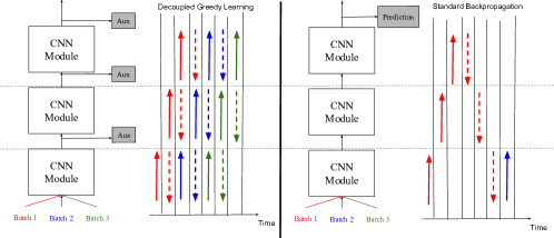
Figure 14: We illustrate the signal propagation for three mini-batches processed by standard back-propagation and with decoupled greedy learning. In each case a module can begin processing forward and backward passes as soon as possible. For illustration we assume same speed for forward and backward passes, and discount the auxiliary network computation (negligible here).

Input: Stream $\mathcal{S}\triangleq\{(x_{0}^{t},y^{t})\}_{t\leq T}$ of samples or mini-batches;

1 Initialize Parameters $\{\theta_{j},\gamma_{j}\}_{j\leq J}$

2 Worker 0:

3 for $x_{0}^{t}\in\mathcal{S}$ do

4       $x^{t}_{1}\leftarrow f_{\theta^{t}_{0}}(x^{t}_{0})$

5       Send $x_{0}^{t}$ to worker $1$

6       Compute $\nabla_{(\gamma_{1},\theta_{1})}\hat{\mathcal{L}}(y^{t},x^{t}_{0};\gamma^{t}_{0},\theta^{t}_{0})$

7       $(\theta^{t+1}_{0},\gamma^{t+1}_{0})\leftarrow$ Step of parameters $(\theta^{t}_{0},\gamma^{t}_{0})$

8 end for

9Worker $j$:

10 for $t\in 0...T$ do

11       Wait until $x^{t}_{j-1}$ is available

12       $x^{t}_{j}\leftarrow f_{\theta^{t}_{j-1}}(x^{t}_{j-1})$

13       Compute $\nabla_{(\gamma_{j},\theta_{j})}\hat{\mathcal{L}}(y^{t},x^{t}_{j};\gamma^{t}_{j},\theta^{t}_{j})$

14       Send $x^{t}_{j}$ to worker $x^{t}_{j+1}$

15       $(\theta^{t+1}_{j},\gamma^{t+1}_{j})\leftarrow$ Step of parameters $(\theta^{t}_{j},\gamma^{t}_{j})$

16 end for

Algorithm 4 DGL Parallel Implementation

Input: Stream $\mathcal{S}\triangleq\{(x_{0}^{t},y^{t})\}_{t\leq T}$; Distribution of the delay $p=\{p_{j}\}_{j}$; Buffer size $M$

1 Initialize: Buffers $\{B_{j}\}_{j}$ with size $M$; params $\{\theta_{j},\gamma_{j}\}_{j}$

2 Worker $j$:

3 while  training do

4       if  $j=1$ then  $(x_{0},y)\leftarrow\mathcal{S}$

5       else  $(x_{j-1},y)\leftarrow B_{j-1}$

6      

7       $x_{j}\leftarrow f_{\theta_{j-1}}(x_{j-1})$

8       Compute $\nabla_{(\gamma_{j},\theta_{j})}\hat{\mathcal{L}}(y,x_{j};\gamma_{j},\theta_{j})$

9       $(\theta_{j},\gamma_{j})\leftarrow$ Step of parameters $(\theta_{j},\gamma_{j})$

10       if $j<J$ then  $B_{j}\leftarrow(x^{j},y)$

11      

12 end while

Algorithm 5 DGL Async Buffer Parallel Impl.

References

- Bartunov et al. (2018) Sergey Bartunov, Adam Santoro, Blake Richards, Luke Marris, Geoffrey E Hinton, and Timothy Lillicrap. Assessing the scalability of biologically-motivated deep learning algorithms and architectures. In Advances in Neural Information Processing Systems, pages 9389–9399, 2018.
- Belilovsky et al. (2019) Eugene Belilovsky, Michael Eickenberg, and Edouard Oyallon. Greedy layerwise learning can scale to imagenet. Proceedings of the 36th International Conference on Machine Learning (ICML), 2019.
- Belilovsky et al. (2020) Eugene Belilovsky, Michael Eickenberg, and Edouard Oyallon. Decoupled greedy learning of cnns. In International Conference on Machine Learning, pages 736–745. PMLR, 2020.
- Bengio et al. (2007) Yoshua Bengio, Pascal Lamblin, Dan Popovici, and Hugo Larochelle. Greedy layer-wise training of deep networks. In Advances in neural information processing systems, pages 153–160, 2007.
- Bottou et al. (2018) Léon Bottou, Frank E Curtis, and Jorge Nocedal. Optimization methods for large-scale machine learning. SIAM Review, 60(2):223–311, 2018.
- Caccia et al. (2020) Lucas Caccia, Eugene Belilovsky, Massimo Caccia, and Joelle Pineau. Online learned continual compression with adaptive quantization modules. Proceedings of the 37th International Conference on Machine Learning, 2020.
- Carreira-Perpinan and Wang (2014) Miguel Carreira-Perpinan and Weiran Wang. Distributed optimization of deeply nested systems. In Artificial Intelligence and Statistics, pages 10–19, 2014.
- Choromanska et al. (2018) Anna Choromanska, Sadhana Kumaravel, Ronny Luss, Irina Rish, Brian Kingsbury, Ravi Tejwani, and Djallel Bouneffouf. Beyond backprop: Alternating minimization with co-activation memory. arXiv preprint arXiv:1806.09077, 2018.
- Czarnecki et al. (2017) Wojciech Marian Czarnecki, Grzegorz Swirszcz, Max Jaderberg, Simon Osindero, Oriol Vinyals, and Koray Kavukcuoglu. Understanding synthetic gradients and decoupled neural interfaces. CoRR, abs/1703.00522, 2017. URL http://arxiv.org/abs/1703.00522.
- Goyal et al. (2017) Priya Goyal, Piotr Dollár, Ross B. Girshick, Pieter Noordhuis, Lukasz Wesolowski, Aapo Kyrola, Andrew Tulloch, Yangqing Jia, and Kaiming He. Accurate, large minibatch SGD: training imagenet in 1 hour. CoRR, abs/1706.02677, 2017. URL http://arxiv.org/abs/1706.02677.
- Haarnoja et al. (2018) Tuomas Haarnoja, Kristian Hartikainen, Pieter Abbeel, and Sergey Levine. Latent space policies for hierarchical reinforcement learning. In Jennifer Dy and Andreas Krause, editors, Proceedings of the 35th International Conference on Machine Learning, volume 80 of Proceedings of Machine Learning Research, pages 1851–1860, Stockholmsmässan, Stockholm Sweden, 10–15 Jul 2018. PMLR. URL http://proceedings.mlr.press/v80/haarnoja18a.html.
- He et al. (2016) Kaiming He, Xiangyu Zhang, Shaoqing Ren, and Jian Sun. Deep residual learning for image recognition. In Proceedings of the IEEE conference on computer vision and pattern recognition, pages 770–778, 2016.
- Huang et al. (2018a) Furong Huang, Jordan Ash, John Langford, and Robert Schapire. Learning deep resnet blocks sequentially using boosting theory. International Conference on Machine Learning(ICML), 2018a.
- Huang et al. (2016) Gao Huang, Yu Sun, Zhuang Liu, Daniel Sedra, and Kilian Q Weinberger. Deep networks with stochastic depth. In European conference on computer vision, pages 646–661. Springer, 2016.
- Huang et al. (2018b) Yanping Huang, Yonglong Cheng, Dehao Chen, HyoukJoong Lee, Jiquan Ngiam, Quoc V Le, and Zhifeng Chen. Gpipe: Efficient training of giant neural networks using pipeline parallelism. arXiv preprint arXiv:1811.06965, 2018b.
- Huo et al. (2018a) Zhouyuan Huo, Bin Gu, and Heng Huang. Training neural networks using features replay. Advances in Neural Information Processing Systems, 2018a.
- Huo et al. (2018b) Zhouyuan Huo, Bin Gu, qian Yang, and Heng Huang. Decoupled parallel backpropagation with convergence guarantee. In Jennifer Dy and Andreas Krause, editors, Proceedings of the 35th International Conference on Machine Learning, volume 80 of Proceedings of Machine Learning Research, pages 2098–2106, Stockholmsmässan, Stockholm Sweden, 10–15 Jul 2018b. PMLR. URL http://proceedings.mlr.press/v80/huo18a.html.
- Ivakhnenko and Lapa (1965) A G Ivakhnenko and V G Lapa. Cybernetic Predicting Devices. CCM Information Corporation., 1965.
- Jaderberg et al. (2017) Max Jaderberg, Wojciech Marian Czarnecki, Simon Osindero, Oriol Vinyals, Alex Graves, David Silver, and Koray Kavukcuoglu. Decoupled neural interfaces using synthetic gradients. International Conference of Machine Learning, 2017.
- Konečnỳ et al. (2015) Jakub Konečnỳ, Brendan McMahan, and Daniel Ramage. Federated optimization: Distributed optimization beyond the datacenter. arXiv preprint arXiv:1511.03575, 2015.
- Krizhevsky (2009) Alex Krizhevsky. Learning multiple layers of features from tiny images. Technical report, Citeseer, 2009.
- Laskin et al. (2020) Michael Laskin, Luke Metz, Seth Nabarrao, Mark Saroufim, Badreddine Noune, Carlo Luschi, Jascha Sohl-Dickstein, and Pieter Abbeel. Parallel training of deep networks with local updates. arXiv preprint arXiv:2012.03837, 2020.
- Leblond et al. (2017) Rémi Leblond, Fabian Pedregosa, and Simon Lacoste-Julien. Asaga: Asynchronous parallel saga. In 20th International Conference on Artificial Intelligence and Statistics (AISTATS) 2017, 2017.
- Leblond et al. (2018) Remi Leblond, Fabian Pedregosa, and Simon Lacoste-Julien. Improved asynchronous parallel optimization analysis for stochastic incremental methods. Journal of Machine Learning Research, 19(81):1–68, 2018. URL http://jmlr.org/papers/v19/17-650.html.
- Lee et al. (2015) Chen-Yu Lee, Saining Xie, Patrick Gallagher, Zhengyou Zhang, and Zhuowen Tu. Deeply-supervised nets. In Artificial intelligence and statistics, pages 562–570, 2015.
- Lee et al. (2014) Dong-Hyun Lee, Saizheng Zhang, Antoine Biard, and Yoshua Bengio. Target propagation. CoRR, abs/1412.7525, 2014. URL http://arxiv.org/abs/1412.7525.
- Lian et al. (2017) Xiangru Lian, Wei Zhang, Ce Zhang, and Ji Liu. Asynchronous decentralized parallel stochastic gradient descent. arXiv preprint arXiv:1710.06952, 2017.
- Lillicrap et al. (2014) Timothy P. Lillicrap, Daniel Cownden, Douglas B. Tweed, and Colin J. Akerman. Random feedback weights support learning in deep neural networks. CoRR, abs/1411.0247, 2014. URL http://arxiv.org/abs/1411.0247.
- Lin (1992) Long-Ji Lin. Self-improving reactive agents based on reinforcement learning, planning and teaching. Machine learning, 8(3-4):293–321, 1992.
- Marquez et al. (2018) E. S. Marquez, J. S. Hare, and M. Niranjan. Deep cascade learning. IEEE Transactions on Neural Networks and Learning Systems, 29(11):5475–5485, Nov 2018. ISSN 2162-237X. doi: 10.1109/TNNLS.2018.2805098.
- Mostafa et al. (2018) Hesham Mostafa, Vishwajith Ramesh, and Gert Cauwenberghs. Deep supervised learning using local errors. Frontiers in neuroscience, 12:608, 2018.
- Nø kland (2016) Arild Nø kland. Direct feedback alignment provides learning in deep neural networks. In D. D. Lee, M. Sugiyama, U. V. Luxburg, I. Guyon, and R. Garnett, editors, Advances in Neural Information Processing Systems 29, pages 1037–1045. 2016.
- Nøkland and Eidnes (2019) Arild Nøkland and Lars Hiller Eidnes. Training neural networks with local error signals. arXiv preprint arXiv:1901.06656, 2019.
- Oord et al. (2017) Aaron van den Oord, Oriol Vinyals, and Koray Kavukcuoglu. Neural discrete representation learning. arXiv preprint arXiv:1711.00937, 2017.
- Ororbia and Mali (2019) Alexander G Ororbia and Ankur Mali. Biologically motivated algorithms for propagating local target representations. In Proceedings of the AAAI Conference on Artificial Intelligence, volume 33, pages 4651–4658, 2019.
- Ororbia et al. (2018) Alexander G Ororbia, Ankur Mali, Daniel Kifer, and C Lee Giles. Conducting credit assignment by aligning local representations. arXiv preprint arXiv:1803.01834, 2018.
- Oyallon (2017) Edouard Oyallon. Building a regular decision boundary with deep networks. In Proceedings of the IEEE Conference on Computer Vision and Pattern Recognition, pages 5106–5114, 2017.
- Oyallon et al. (2018) Edouard Oyallon, Eugene Belilovsky, Sergey Zagoruyko, and Michal Valko. Compressing the input for cnns with the first-order scattering transform. In Proceedings of the European Conference on Computer Vision (ECCV), pages 301–316, 2018.
- Simonyan and Zisserman (2014) Karen Simonyan and Andrew Zisserman. Very deep convolutional networks for large-scale image recognition. arXiv preprint arXiv:1409.1556, 2014.
- Taylor et al. (2016) Gavin Taylor, Ryan Burmeister, Zheng Xu, Bharat Singh, Ankit Patel, and Tom Goldstein. Training neural networks without gradients: A scalable admm approach. In Maria Florina Balcan and Kilian Q. Weinberger, editors, Proceedings of The 33rd International Conference on Machine Learning, volume 48 of Proceedings of Machine Learning Research, pages 2722–2731, New York, New York, USA, 20–22 Jun 2016. PMLR. URL http://proceedings.mlr.press/v48/taylor16.html.
- van den Oord et al. (2017) Aäron van den Oord, Oriol Vinyals, and Koray Kavukcuoglu. Neural discrete representation learning. In NIPS, 2017.
- Verma et al. (2018) Vikas Verma, Alex Lamb, Christopher Beckham, Amir Najafi, Aaron Courville, Ioannis Mitliagkas, and Yoshua Bengio. Manifold mixup: Learning better representations by interpolating hidden states. 2018.
- Xiao et al. (2019) Will Xiao, Honglin Chen, Qianli Liao, and Tomaso A. Poggio. Biologically-plausible learning algorithms can scale to large datasets. International Conference on Learning Representations, 2019.
- Zagoruyko and Komodakis (2016) Sergey Zagoruyko and Nikos Komodakis. Wide residual networks. arXiv preprint arXiv:1605.07146, 2016.
- Zhang et al. (2015) Sixin Zhang, Anna E Choromanska, and Yann LeCun. Deep learning with elastic averaging sgd. In C. Cortes, N. D. Lawrence, D. D. Lee, M. Sugiyama, and R. Garnett, editors, Advances in Neural Information Processing Systems 28, pages 685–693. Curran Associates, Inc., 2015.