Projection-based resolved interface mixed-dimension method for embedded tubular network systems

Abstract

We present a flexible discretization technique for computational models of thin tubular networks embedded in a bulk domain, for example a porous medium. These systems occur in the simulation of fluid flow in vascularized biological tissue, root water and nutrient uptake in soil, hydrological or petroleum wells in rock formations, or heat transport in micro-cooling devices. The key processes, such as heat and mass transfer, are usually dominated by the exchange between the network system and the embedding domain. By explicitly resolving the interface between these domains with the computational mesh, we can accurately describe these processes. The network is efficiently described by a network of line segments. Coupling terms are evaluated by projection of the interface variables. The new method is naturally applicable for nonlinear and time-dependent problems and can therefore be used as a reference method in the development of novel implicit interface 1D-3D methods and in the design of verification benchmarks for embedded tubular network methods. Implicit interface, not resolving the bulk-network interface explicitly have proven to be very efficient but have only been mathematically analyzed for linear elliptic problems so far. Using two application scenarios, fluid perfusion of vascularized tissue and root water uptake from soil, we investigate the effect of some common modeling assumptions of implicit interface methods numerically.

1 Introduction

Figure 1: Examples of systems with embedded network structures. Left, blood vessel network simulation (geometry and boundary conditions from [1]) in the rat brain cortex coupled with the embedding tissue. Color signifies simulated blood pressure. A grey matter tissue volume of $1\text{\,}{\mathrm{mm}}^{3}$ may contain around 10’000 blood vessels. Right, simulation of root water and tracer uptake from soil by a young lupine root system, image adapted from [2] (license: CC BY 4.0).

There is a strong demand for efficient and accurate models describing flow and transport processes in porous media with embedded tubular network systems, such as vascularized biological tissue, plant root system growing in soil, hydrological, geothermal or petroleum wells in rock formations. Reduced models are necessary due to the computational complexity arising from the large number of network segments (for example about 10’000 blood vessels in a $1\text{\,}{\mathrm{mm}}^{3}$ cube of gray matter brain tissue [3], or hundreds of meters of cumulative root length in a $60$-day-old maize root system [4]) and the small diameter of the tubes with respect to the entire computational domain (for example wells of $10\text{\,}\mathrm{cm}$ diameter in a $\mathrm{km}$-scale reservoir). Two motivational examples of mixed-dimensional simulations are shown in Fig. 1.

Various methods have been developed recently to numerically solve coupled mixed-dimensional partial differential equations (PDEs) that arise from flow and transport models in such systems. Typically, flow and transport in the embedded tubular network system are described by one-dimensional equations posed on a network of (center-)line segments. These networks are embedded into the surrounding bulk medium, often porous media, which are described by three-dimensional equations. Network and bulk PDEs are coupled by source terms that depend on state variables from both domains. The different numerical techniques differ in the way they deal with the dimensional gap of $2$ between network and bulk domain. The source term contribution in the embedding bulk medium can be described by line source terms [5, 6, 7, 8, 9], surface source terms [10, 11] or volume source terms [12].

A common assumption of mixed-dimensional models is that the radial scale of network tubes $R$ is much smaller than the dimension $\lvert{\Omega}\rvert$ of the domain of interest $\Omega$. More specifically for network systems, $R$ has to be much smaller than the average distance to the closest neighboring segment in the network. While this precondition may be clearly satisfied in some cases (e.g. simple injection and extraction wells in large distance to each other), it is less clear in others (blood capillaries with $38\text{\,}\mathrm{\SIUnitSymbolMicro m}$ vessel radius with average distances of $50\text{\,}\mathrm{\SIUnitSymbolMicro m}$ in a microvascular network occupying about $23\text{\,}\mathrm{\char 37\relax}$ of the tissue volume). Based on this main assumption, a couple of arguments are derived leading to the simplification of the model equations. To allow for simple meshing procedure independent of the network domain, the three-dimensional domain is extended to also cover the volume occupied by the tubular network geometry [11]. This means the volume of the three-dimensional domain is overestimated. Moreover, the tubes do not pose any resistance to flow since the physical presence of the tubes is removed. Finally, since these mixed-dimension models are usually derived for infinite cylindrical segments, some error is involved at bifurcations by assuming finite cylindrical segments. In this work, we want to investigate some of these assumptions numerically in more detail than previously presented.

The mentioned mixed-dimensional models have been derived in the context of linear elliptic PDEs with line source terms. Extensions to time-dependent problems and nonlinear problems have been analyzed to a much less extent. Mixed-dimension methods are for example used to describe root water uptake from soil, in which case the soil is described by the Richards equation—a strongly nonlinear PDE. Although simple mixed-dimension methods have been used for more than two decades root water uptake simulations [13], the proper grid resolution required to accurately solve the model equations in dry soils is rarely considered in the literature [14, 15]. It is known that a coarse grid resolution in the soil domain may not accurately approximate local pressure gradients and models for the root water uptake flux correction have been developed [16, 17, 18]. To the best of our knowledge, the coupled root water uptake problem has not been rigorously analyzed mathematically. The estimation of discretization errors and possible errors in the model reduction are yet to be better understood. In this work we present a model technique to investigate such errors numerically.

In previous works on tissue perfusion models [6] and in more general mathematical works [19], it has been found that mixed-dimension embedded schemes exhibit sub-optimal convergence rates, if the local discretization length $h$ is larger than the radius $R$ of the embedded vessels. While convergence rates alone are inconclusive about the error at a given practical discretization length, the results in [19, 10, 12] indicate that in order to achieve sufficiently accurate numerical results, the discretization length in the embedding bulk domain has to be chosen in the order of the network tube radii or smaller. This is in stark contrast to typical grid resolutions in root water uptake simulations, where soil cells are routinely chosen an order of magnitude larger than the root radius [14, 4]. Several techniques to relax this discretization length restriction have been discussed in the context of linear stationary elliptic mixed-dimensional equations [9, 12, 20].

In this work, we present a method where the tubular network is described by a network of line segments with a given radius function as common in mixed-dimensional models. However, we explicitly resolve the interface of the tubular network with the computational mesh describing the embedding bulk domain. The new interface-resolving method developed subsequently can be considered a reference method for the comparison of efficient mixed-dimension embedded schemes based on implicit or reduced interface concepts.

For reference, we mention that in root-soil interaction simulations, the root-soil interface has been explicitly resolved based on imaging data in a recent work by Daly2018 [21]. However, only flow in the soil is simulated and the flow field is not coupled to the flow field in the root xylem. Consequently, it is necessary to specify boundary conditions on the root-soil interface. For the subsequently introduced method, the state of the root-soil interface is part of the solution. Finally, we briefly introduced the new method in [22], where it is suggested for the purpose of providing a reference solution in a benchmark study for root water uptake simulators. In this work, we describe and analyse the method in more detail.

The new numerical method is derived in Section 2 (mathematical model) and Section 2.3 (discretization aspects) and then applied in several numerical cases in Section 3. A grid convergence study in Section 3.1 shows that the method is more accurate than other mixed-dimension methods for similar mesh sizes. We compare the new method with previously published methods for examples for numerical test cases of tissue perfusion and root water uptake in Sections 3.2 and 3.3.

2 Mixed-dimension method with resolved interface

Figure 2: Embedded tubular network system. A tubular network structure with centerline skeleton $\Lambda$ is embedded into the bulk domain $\Omega$. The surface of the tubes $\Gamma$ (dark grey) forms an internal boundary for $\Omega$, $\Gamma\subset\Omega\cap\mho$. Both domains are equipped with (local) coordinate systems. $R=R(s)$ denotes the equivalent local radius of the tube.

The tubular segments in network systems like plant roots or capillary blood vessels are usually much smaller in radial extent than in axial extent, $R\ll L$. Often, it is therefore a good assumption to neglect radial variations and work with cross-section averaged quantities and one-dimensional models that describe the change of e.g. average pressure, temperature, concentration, etc. along the centerline axis [23]. In this work we will assume that this one-dimensional description is sufficiently accurate and exploit this fact by not resolving the network structure with a fully-resolved three-dimensional computational mesh which would result in problems of intractable size. Moreover, we assume that any membrane separating the internal highly conducting space of the tube (e.g. blood vessel lumen, root xylem) from the bulk domain can be described as a two-dimensional sharp interface $\Gamma$.

In the following, we will exemplarily consider the case of root water uptake. For details on the mathematical modeling of root water uptake with three-dimensional root architectures, we refer to the literature [13, 24, 25, 26, 27, 22]. Fluid flow in the root xylem—a structure that can be imagined as a bundle of tubes located in the center of the root and transporting fluid in axial direction upwards toward the plant leaves—can be described by

$$-{\partial_{s}}\left(K_{\text{ax}}{\partial_{s}}p_{\mathrm{1D}}\right)=-q\quad\text{on}\quad\Lambda,$$ (2.1)

with some boundary conditions on $\partial\Lambda$, where $s$ denotes the local axial coordinate, $K_{\text{ax}}$ (in ${\mathrm{m}}^{4}\text{\,}{\mathrm{Pa}}^{-1}\text{\,}{\mathrm{s}}^{-1}$) is the axial root xylem conductivity, $p_{\mathrm{1D}}$ is the root xylem pressure (in $\mathrm{Pa}$), and $q$ (in ${\mathrm{m}}^{2}\text{\,}{\mathrm{s}}^{-1}$) is a source term modeling fluid exchange with the embedding soil domain and depends on both $p_{\mathrm{1D}}$ and the soil pressure $p_{\mathrm{3D}}$ on the interface $\Gamma$.

Water flow in the soil is described by the Richards equation,

$$-\nabla\cdot\!\left(\frac{k_{r}(p_{\mathrm{3D}})}{\mu}K\nabla\!p_{\mathrm{3D}}+\rho\boldsymbol{g}\right) =0 \text{in}\quad\Omega,$$ (2.2)

$$-\left(\frac{k_{r}(p_{\mathrm{3D}})}{\mu}K\nabla\!p_{\mathrm{3D}}+\rho\boldsymbol{g}\right)\cdot\boldsymbol{n}_{\Gamma} =K_{\text{r}}\left[p_{\mathrm{3D}}(\boldsymbol{x}_{\Gamma})-p_{\mathrm{1D}}(\Pi\boldsymbol{x}_{\Gamma})\right] \text{on}\quad\Gamma,$$ (2.3)

with suitable boundary conditions prescribed on $\partial\Omega\setminus\Gamma$. In Eq. 2.2, $\mu$ is the dynamic fluid viscosity (in $\mathrm{Pa}\text{\,}\mathrm{s}$), $\rho$ is the fluid density (in $\mathrm{kg}\text{\,}{\mathrm{m}}^{-3}$), $k_{r}$ denotes the dimensionless relative permeability, and $K$ the intrinsic permeability of the soil (in ${\mathrm{m}}^{2}$). The relative permeability is a nonlinear function of $p_{\mathrm{3D}}$, e.g. modeled by the well-known Van Genuchten-Mualem model [28, 29]. In Eq. 2.3, $\boldsymbol{n}_{\Gamma}$ is an outward-pointing (with respect to $\Omega$) unit normal on $\Gamma$ and $K_{r}$ is the radial root conductivity (in $\mathrm{m}\text{\,}{\mathrm{Pa}}^{-1}\text{\,}{\mathrm{s}}^{-1}$). Finally, $\Pi\bullet$ is a surjective projection operator that maps any point $\boldsymbol{x}_{\Gamma}$ on $\Gamma$ to a corresponding point $\hat{s}$ on $\Lambda$, given a parameterization of $\Lambda$ in terms of $\hat{s}$.

In order to obtain a mass conservative coupling scheme, we need to define the source term $q$ in Eq. 2.1. To this end, we denote with $\Lambda_{\varsigma}\subseteq\Lambda$ some compact subset of $\Lambda$ and with $\Gamma_{\varsigma}=\{\boldsymbol{x}_{\Gamma}\in\Gamma\mid\Pi\boldsymbol{x}_{\Gamma}\in\Lambda_{\varsigma}\}$ the corresponding set of surface points on $\Gamma$. Then, the coupling condition is given by

$$\begin{split}\int_{\Lambda_{\varsigma}}\!q\,\text{d}s&=\int_{\Gamma_{\varsigma}}\!\left(\frac{k_{r}(p_{\mathrm{3D}})}{\mu}K\nabla\!p_{\mathrm{3D}}+\rho\boldsymbol{g}\right)\cdot\boldsymbol{n}_{\Gamma}\,\text{d}\gamma\\ &=\int_{\Gamma_{\varsigma}}\!-K_{\text{r}}\left[p_{\mathrm{3D}}(\boldsymbol{x}_{\Gamma})-p_{\mathrm{1D}}(\Pi\boldsymbol{x}_{\Gamma})\right]\,\text{d}\gamma,\end{split}$$ (2.4)

given some suitable parameterization of $\Gamma_{\varsigma}$ in terms of $\gamma$.

2.1 Practical geometry parameterization

Figure 3: Three-dimensional representations of a segmented root architecture (lupine). From right to left: graph representation with segment-wise continuous radius field, implicit geometrical representation as the sum of capsules, and discrete representation of root-soil interface as the surface facets of a tetrahedron mesh of the soil domain (generated with CGAL [30]).

The interface $\Gamma$ between network and bulk domain may often be given by some implicit description in form of a continuous or discrete level set function, e.g. obtained from imaging data. From such an implicit description it is possible to generate surface triangulations [31], and extract center-lines, for example based on the medial axis transformation [32, 33]. Nevertheless, there is in general no unique choice for the mapping $\Pi$.

Since our method is targeted at the creation of verification tests for reduced methods without explicit interface resolution, we simplify the geometrical description as follows. The root network center-lines $\Lambda$ are approximated by $\Lambda_{h}$, a set of linear root segment center-lines $\Lambda_{i}$ defined by two points $\boldsymbol{q}_{i}$, $\boldsymbol{p}_{i}$ and parametrized by

$$\tilde{\boldsymbol{x}}(\tilde{s}_{i}):=\boldsymbol{p}_{i}+\tilde{s}_{i}\boldsymbol{m}_{i},\quad\boldsymbol{m}_{i}=\boldsymbol{q}_{i}-\boldsymbol{p}_{i},\quad\text{for}\quad\tilde{s}_{i}\in[0,1].$$ (2.5)

Moreover, associated which each segment is a continuous radius function $R_{i}(\tilde{s}_{i})$ which is often—but not necessarily—constant per segment but varies from segment to segment. From this representation, we implicitly define a three-dimensional network representation by the signed distance functions (SDFs),

$$\begin{split}d_{\Lambda_{h}}(\boldsymbol{x})&:=\min\limits_{\Lambda_{i}\in\Lambda_{h}}d_{\Lambda_{i}}(\boldsymbol{x}),\quad\boldsymbol{x}\in\mathbb{R}^{3},\\ d_{\Lambda_{i}}(\boldsymbol{x})&:=\|\tilde{\boldsymbol{x}}(\mathbb{P}_{i}(\boldsymbol{x}))-\boldsymbol{x}\|-R_{i}(\mathbb{P}_{i}(\boldsymbol{x})),\\ &\text{where}\quad\hat{s}_{i}:=\mathbb{P}_{i}(\boldsymbol{x})=\max\left\{0,\min\left\{\frac{(\boldsymbol{x}-\boldsymbol{p}_{i})\cdot\boldsymbol{m}_{i}}{\lVert\boldsymbol{m}_{i}\rVert^{2}_{2}},1\right\}\right\}.\end{split}$$ (2.6)

This parameterization allows for the convenient definition of the operator $\Pi$ to yield the position $\hat{s}_{i}$ on the segment $\Lambda_{i}$ with minimal $d_{\Lambda_{i}}(\boldsymbol{x})$.

Remark.

The SDFs $d_{\Lambda_{i}}$ describe capsules with radius function $R_{i}(\tilde{s}_{i})$ around the line $\Lambda_{i}$ and the SDF $d_{\Lambda_{h}}$ describes the union of all such capsules. Then every point $\boldsymbol{x}$ is inside the root, if $d_{\Lambda_{h}}(\boldsymbol{x})<0$, or in the soil or outside the domain, if $d_{\Lambda_{h}}(\boldsymbol{x})>0$. Consequently, the root-soil surface is given by the zero level set $\Gamma=\{\boldsymbol{x}\,|\,d_{\Lambda_{h}}(\boldsymbol{x})=0\}$.

In this work, we use the meshing capabilities of the C++ geometry library CGAL [30] to generate computational grids for the bulk domain from such an implicit description. These grid explicitly resolve the bulk-network interface. An exemplary root network, the three-dimensional representation as a union of capsules, and a triangulated representation of $\Gamma$ is shown in Fig. 3.

We note that the surface implied by the zero level set of Eq. 2.6 is only piecewise differentiable due to the possible discontinuity of $R$ between segments. If necessary, the surface’s smoothness can be improved by using a smooth minimum function for $d_{\Lambda_{h}}$, such as

$$\operatorname{smin}(a,b,k):=\min\{a,b\}-\frac{1}{6}h^{3}k,\quad h=\frac{1}{k}\max\{k-|a-b|,0\},$$ (2.7)

rendering the surface function twice differentiable ($C^{2}$) [34]. The parameters $a$ and $b$ are signed distances and $k>0$ is a smoothing parameter (with units $\mathrm{m}$) which is to be chosen in the order of magnitude of the dimensions of the objects merged. In the following, we do not perform such smoothing of the network surface, and approximate the surface by the zero level set of the distance function Eq. 2.6.

2.2 Relation to implicit surface mixed-dimension methods

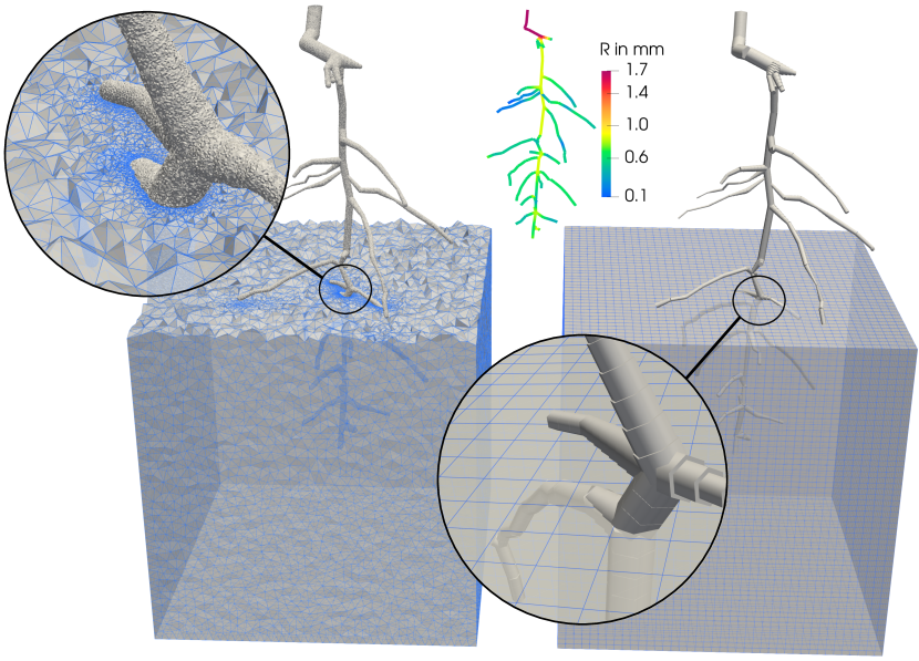
Figure 4: Comparison of two mixed-dimension discretization concepts. A root system is embedded in a soil domain. Left, resolved-interface discretization. Coupling terms appear as boundary conditions for the 3D bulk domain. Right, implicit interface method with non-matching discretization. The bulk domain is extended to include the space occupied by the network (in its three-dimensional representation). Coupling terms for each segment appear as source terms restricted to a line [6], a local surface [10], or a local volume [12], depending on the chosen method. This approach introduces additional model errors but implicit interface methods are expected to be computationally more efficient than the resolved-interface approach.

With the parameterization introduced in Section 2.1, consider a circular cross-section of radius $R_{i}$ of an infinite cylindrical tube. Then, we can show that

$$q(\tilde{s}_{i}) =\int_{0}^{2\pi}\!-K_{r}\left(p_{\mathrm{3D}}(\boldsymbol{x})-p_{\mathrm{1D}}(\Pi\boldsymbol{x})\right)R_{i}\text{d}\theta$$

$$=-2\pi R_{i}K_{r}\left(\frac{1}{2\pi}\int_{0}^{2\pi}\!p_{\mathrm{3D}}(\boldsymbol{x})\,\text{d}\theta-\frac{1}{2\pi}\int_{0}^{2\pi}\!p_{\mathrm{1D}}(\Pi\boldsymbol{x})\,\text{d}\theta\right)$$

$$=-2\pi R_{i}K_{r}\left(\hat{p}^{\bigcirc}_{\mathrm{3D}}-p_{\mathrm{1D}}(\tilde{s}_{i})\right),$$ (2.8)

where we used the fact that $p_{\mathrm{1D}}$ is independent of $\theta$, and define the average pressure on the perimeter as

$$\hat{p}^{\bigcirc}_{\mathrm{3D}}:=\frac{1}{2\pi}\int_{0}^{2\pi}\!p_{\mathrm{3D}}(\boldsymbol{x})\,\text{d}\theta.$$ (2.9)

Hence, if the network is approximated by sufficiently long discrete cylinder segments and exchange is assumed to only occur over the lateral surface of the cylinders, the source term can be formulated solely in terms of quantities on the cross-sectional plane. Furthermore, assuming that the network domain does not pose any resistance to flow in the bulk domain and its volume is negligible, $\Omega$ is extended to include the network domain, $\Omega^{\text{ex}}=\Omega\cup\mho$, and we arrive at a reduced model that can be written in terms of a delta distribution restricting the bulk source term onto $\Gamma$, cf. [10],

$$-\nabla\cdot\!\left(\frac{k_{r}(p_{\mathrm{3D}})}{\mu}K\nabla\!p_{\mathrm{3D}}\right) =q\delta_{\Gamma} \text{in}\quad\Omega^{\text{ex}},$$ (2.10)

$$-{\partial_{s}}\left(K_{\text{ax}}{\partial_{s}}p_{\mathrm{1D}}\right) =-q \text{on}\quad\Lambda,$$ (2.11)

$$q =-2\pi RK_{\text{r}}(\hat{p}_{\mathrm{3D}}^{\bigcirc}-p_{\mathrm{1D}}),$$ (2.12)

$$\int_{\Omega^{\text{ex}}}\!q\delta_{\Gamma}\,\text{d}\boldsymbol{x} =\int_{\Gamma}\!\frac{q}{2\pi R}\,\text{d}\gamma=\int_{\Lambda}\!q\,\text{d}s.$$ (2.13)

In the following, we refer to such formulations as implicit surface methods as the exchange between bulk domain and network is entirely formulated in terms of source terms in $\Omega^{\text{ex}}$ instead of boundary conditions on $\Gamma$ and an explicit resolution of the bulk-network interface by the computational mesh of the bulk domain is not necessary anymore. However, we note that the interface $\Gamma$ still appears implicitly in form of the delta distribution. Figure 4 compares the meshes used for resolved-interface descriptions and implicit interface description in non-matching discretization schemes.

In [35], the author suggests to use $\delta_{\Lambda}$ instead of $\delta_{\Gamma}$ in Eq. 2.10, i.e. the source term is restricted to a line in $\Omega^{\text{ex}}$. This formulation results in pressure solutions with feature singularities on $\Lambda$ and are difficult to approximate by numerical schemes. In [12], the authors suggest to replace the surface source term by a volume source term using a distribution kernel in combination with a local reconstruction scheme of the interface pressure $\hat{p}_{\mathrm{3D}}^{\bigcirc}$. This technique allows to decouple the discretization length from the tube radius, but the local reconstruction scheme has only been investigated for linear problems so far (corresponding to a constant relative permeability $k_{r}$ in Eq. 2.10). In Section 3, we compare the new resolved-interface method with implicit interface methods in numerical experiments. To this end, we follow the terminology of [12] and refer with css (cylinder surface source) to the method due to [10] using formulation Eqs. 2.10, 2.11 and 2.12. We refer with ls (line source) to the method due to [35] where $\delta_{\Gamma}$ is replaced by $\delta_{\Lambda}$, and with ds (distributed source) to the method due to [12], where $\delta_{\Gamma}$ is replaced by a volumetric distribution kernel and the source term $q$ is computed based on a local reconstruction scheme.

2.3 Integration of the coupling term

In the discrete setting, the root and the soil domain, $\Lambda$ and $\Omega$ are partitioned into a finite number of grid cells such that $\Lambda_{h}=\bigcup K_{\Lambda}$ and $\Omega_{h}=\bigcup K_{\Omega}$ are discrete mesh representations of $\Lambda$ and $\Omega$ with the cells $K_{\Lambda}$ and $K_{\Omega}$. The computational grids can be chosen independently. A part of the boundary of $\Omega$ explicitly resolves the root-soil interface $\Gamma$ and $\Gamma_{h}$ denotes the set of cell facets on the interface. Since the interface is explicitly described by $\Gamma_{h}$, the the coupling conditions, Eq. 2.3, can be directly evaluated by numerically approximating the surface integrals. However, in the discrete setting, the approximation of $p_{\mathrm{3D}}$ is typically only piecewise differentiable. In this work, we consider piecewise linear functions. The source term $q$ needs to be integrated over a control volume $K_{\Lambda}$ which may involve integration over several interface facets. For this purpose, we suggest an algorithm based on virtual local refinement of the interface facets to accurately capture the surface integration area element associated with the integration over $K_{\Lambda}$. The algorithm is given as pseudo-code in Algorithm 1. In brief, we map the corners of a surface triangle with $\Pi$ and evaluate if the mapped points are contained in different network control volumes. If so, the triangle is virtually refined and the procedure is repeated recursively until all corners map to the same control volumes, or some maximum refinement level is reached. We add only one integration point per surface triangle and coupled network control volume at the centroid of the union of coupled sub-triangles. For $p_{\mathrm{3D}}$ and $p_{\mathrm{1D}}$ being piecewise linear functions, integrating with the mid-point rule is exact.

3 Numerical results and discussion

In this section, we compare the introduced explicit interface method with previously suggested implicit interface methods in three cases. We use the abbreviations ls, css, ds introduced in Section 2.2 for the implicit interface methods and abbreviate with ps (projection source) the explicit interface method. In the first case, Section 3.1, we show for a simple rotation-symmetric setup with a single tubular inclusion that ps accurately approximates a given analytical solution and verify that the surface integration scheme proposed in Section 2.3 is sufficiently accurate. In the second case, Section 3.2, we investigate errors introduced by implicit interface methods at the example of tissue perfusion described by a linear elliptic mixed-dimensional model. In the third case, Section 3.3, we investigate differences between ps and css in a root water uptake example described by a nonlinear elliptic mixed-dimension model based on the Richards equations.

The three-dimensional bulk domains $\Omega$, $\Omega^{\text{ex}}$ and the network domain $\Lambda$ are spatially decomposed into the meshes $\Omega_{h}$, $\Omega_{h}^{\text{ex}}$ and $\Lambda_{h}$ consisting of cells $K_{\Omega}\in\Omega_{h}$ and $K_{\Lambda}\in\Lambda_{h}$, respectively. The discretization length computed as the maximal cell diameter is denoted by $h$. We discretize the continuous equation in space using finite volume methods. For structured Cartesian grids as well as for the network equations, we use a cell-centered finite volume method (fvm) with a two-point flux approximation (tpfa), cf. [12]. When using (unstructured) tetrahedral meshes for the ps method, or in the case of locally refined meshes for the css method in Section 3.3, we use vertex-centered finite volumes with linear basis functions (also referred to as box method) [36, 37, 2]. This is because cell-centered tpfa-fvm are generally not consistent on such meshes [38]. The resulting discrete system of equations is solved with Newton’s method. (In case of a linear model Newton’s method converges in one step.) The linearized system of equations within each Newton iteration, is solved with a stabilized bi-conjugate gradient method using a block-diagonal preconditioner based on incomplete LU-factorization, cf. [12]. All presented methods and simulations are implemented using the open-source software framework DuMu^x [2] with the network grid implementation dune-foamgrid [39] for representing the embedded network domain.

3.1 Mixed-dimension single phase flow

Figure 5: Reference solution for an embedded cylinder. Cylindrical tube embedded in a box-shaped domain with dimensions $[-1,1]\times[-1,1]\times[-1,1]$. The domain is cut in half revealing the tube of radius $R=0.03$ visualized with a reduced radius to make the interface visible. The numerical solutions $p_{\mathrm{3D}}^{\textsc{ps}}$, $p_{\mathrm{1D}}^{\textsc{ps}}$ computed on a fine grid with $h=0.008$ are shown exemplarily but they are visually identical to a plot of the analytical solution.

Figure 6: Convergence rates over discretization length.

Let us consider a slightly simplified problem, adapted from d2007multiscale [35, 12], (for simplicity we use the same symbols as previously introduced but all unknowns and parameters are to be interpreted as dimensionless quantities,)

$$-\partial_{s}\left(K_{\text{ax}}\partial_{s}p_{\mathrm{1D}}\right) =-q\quad \text{in }\Lambda,$$ (3.1a)

$$-\nabla\cdot\!(\nabla\!p_{\mathrm{3D}}) =q\delta_{\Lambda}\quad \text{in }\Omega^{\text{ex}},$$ (3.1b)

$$q =-2\pi RK_{r}(\hat{p}_{\mathrm{3D}}^{\bigcirc}-p_{\mathrm{1D}}),$$ (3.1c)

with the domains $\Omega^{\text{ex}}=[-1,1]\times[-1,1]\times[-1,1]$ and $\Lambda=\{0\}\times\{0\}\times[0,1]$, i.e the vessel center-line coincides with the $x_{3}$-axis. The tube has radius $R$ and $\mho$ is given by the cylinder with center-line $\Lambda$, radius $R$ and unit length. Recall that for this straight cylindrical tube case, due to the observation in Section 2.2, problem formulation Eq. 3.1 is equivalent to the formulation with boundary conditions on $\Gamma$, cf. Eqs. 2.1, 2.2 and 2.3 and

$$\int_{\Lambda}\!q\,\text{d}s=\int_{\Omega^{\text{ex}}}\!q\delta_{\Lambda}\,\text{d}x=\int_{\Gamma}\!-K_{\text{r}}\left[p_{\mathrm{3D}}(\boldsymbol{x}_{\Gamma})-p_{\mathrm{1D}}(\Pi\boldsymbol{x}_{\Gamma})\right]\,\text{d}\gamma.$$ (3.2)

Choosing the conductivities as

$$K_{\text{ax}}=1+x_{3}+\frac{1}{2}x_{3}^{2},\quad K_{r}=\left(2\pi R+R\ln{R}\right)^{-1},$$

the pressure solutions,

$$p_{\mathrm{1D},\mathrm{e}}=1+x_{3},\quad p_{\mathrm{3D},\mathrm{e}}=-\frac{1+x_{3}}{2\pi}\ln r,\quad r\geq R$$ (3.3)

with $r=\sqrt{x_{1}^{2}+x_{2}^{2}}$, solve Eq. 3.1 with matching boundary conditions. From the analytical pressure solutions follows that $q_{\mathrm{e}}=1+x_{3}$ is the analytical source term.

In this setting, we can directly compare the explicit interface method with implicit interface methods. The analytical solutions $p_{\mathrm{1D},\mathrm{e}}$ and $q_{\mathrm{e}}$ are identical for all mentioned methods, cf. [12]. The exact pressure in the bulk domain, $p_{\mathrm{3D},\mathrm{e}}$, can be extended to all of $\Omega^{\text{ex}}$ and differs between the different methods for $r<R$ (and $r<\varrho$ for the distributed source method (ds) of [12] where $\varrho$ is the radius of the distribution kernel), but is identical for $r\geq R$ ($r\geq\varrho$ for ds). The analytical solutions $p_{\mathrm{3D},\mathrm{e}}^{\textsc{m}}\in\Omega^{\text{ex}}$ for the methods $M\in\{\textsc{ls},\textsc{css},\textsc{ds}\}$ are given in Appendix B.

For the resolved interface method ps, in the case of straight cylindrical vessels, integration of the source term $q_{K_{\Lambda}}$ over the discrete interface $\Gamma_{h}$ can be performed exactly. To this end, we compute for every segment $K_{\Lambda}$ the intersections of the space between the two planes implied the segment $K_{\Lambda}$ (the two planes through the end points and normal to the segment) and all surface triangles $T\in\Gamma_{h}$. Effectively, every $T$ is sub-triangulated such that every sub-triangle couples with exactly one $K_{\Lambda}$. The boundary integral can be computed by the mid-point rule which is exact since the integrand is a linear function. Intersections cannot be so easily computed in networks where the interface is only given as an implicit function. Therefore, we suggested an approximate integration algorithm based on virtual refinement in Section 2.3. For this particular test case, we implemented both approaches to verify the accuracy of the latter. We denote the exact approach with ps-e and the approximate approach with ps-a.

We solve Eq. 3.1 with the methods ls, css, ds, ps-e and ps-a and by prescribing the analytical solutions as Dirichlet boundary conditions, except for the top and bottom sections of $\Omega$ or $\Omega^{ex}$ ($x_{3}=0$, $x_{3}=1$) where we prescribe the normal derivative of the analytical solution as Neumann boundary condition. Obviously, for the methods ps-e and ps-a, $\Gamma$ does not require boundary conditions and fluxes over $\Gamma$ are computed by the coupling conditions, Eq. 3.2. The numerical solutions $p^{\textsc{ps}}_{\mathrm{3D}}$ and $p_{\mathrm{1D}}$ for ${R}=0.03$ are shown in Fig. 5.

We compute pressure discretization errors in the normalized discrete norm

$$\lVert p_{\mathrm{3D}}-p^{\textsc{m}}_{\mathrm{3D},\mathrm{e}}\rVert_{2}:=\frac{\left[\sum_{\Omega_{h}}|K_{\Omega}|(p^{\textsc{m}}_{K_{\Omega},\mathrm{e}}-p_{K_{\Omega}})^{2}\right]^{1/2}}{\sum_{\Omega_{h}}|K_{\Omega}|},$$ (3.4)

where $p_{K_{\Omega}}$, $p_{K_{\Omega},\mathrm{e}}$ denote numerical and exact pressure evaluated at the center of a control volume $K_{\Omega}$ and $|K_{\Omega}|$ its volume. The error for $p_{\mathrm{1D}}$ in $\Lambda_{h}$ is computed analogously. The error in the source term $q$ is computed as

$$\lVert q-q_{e}\rVert_{2}=\frac{\left[\sum_{\Lambda_{h}}|K_{\Lambda}|(q_{K_{\Lambda},\mathrm{e}}-q_{K_{\Lambda}})^{2}\right]^{1/2}}{\sum_{\Lambda_{h}}|K_{\Lambda}|},$$ (3.5)

where

$$q_{K_{\Lambda},\mathrm{e}}=\int_{K_{\Lambda}}\!q_{\mathrm{e}}\,\text{d}s\quad\text{and}\quad q_{K_{\Lambda}}=\int_{K_{\Lambda}}\!q\,\text{d}s.$$ (3.6)

The maximum control volume size, $h$, is given by the maximum cell diameter in both domains. We choose $h=h_{\Omega}$ such that $h_{\Omega}\approx h_{\Lambda}$. Both domains are uniformly refined. The mesh for ps is remeshed so that the discrete interface $\Gamma_{h}$ approaches the real interface $\Gamma$ with grid refinement. Pressure and source error norms with grid refinement are shown in Fig. 6.

For sufficiently smooth solutions, the employed finite volume schemes are expected to show a quadratic error decay of both pressures with grid refinement in the specified discrete norms. However, $p_{\mathrm{3D},\mathrm{e}}^{\textsc{ls}}$ exhibits a singularity for all $\boldsymbol{x}\in\Lambda$ and $p_{\mathrm{3D},\mathrm{e}}^{\textsc{css}}$ has a kink on $\Gamma$. Therefore, the convergence rate is reduced for these methods. Unfortunately, for the ls method the convergence order of $p_{\mathrm{1D},\mathrm{e}}^{\textsc{ls}}$ is affected by the reduced convergence order of $p_{\mathrm{3D},\mathrm{e}}^{\textsc{ls}}$.

It is evident from the convergence results that for a given grid resolution the ps method shows the smallest error of all presented methods. Furthermore, the integration scheme suggested in Section 2.3 (ps-a) is accurate enough and matches the results with the exact integration formula (ps-e) well. This motivates the conclusion that the newly introduced explicit interface method may serve as a reference for implicit interface methods.

3.2 Fluid perfusion of vascularized tissue

Fluid flow in the capillary blood vessels, in the (fluid-filled) extra-vascular extra-cellular space (interstitium), and fluid exchange between these compartments can be described by linear mixed-dimensional PDE systems [6, 8, 12]. In this section, we consider the following model:

$$-\partial_{s}\left(K_{\text{ax}}\partial_{s}p_{\mathrm{1D}}\right) =-q \text{on}\quad\Lambda,$$ (3.7a)

$$-\nabla\cdot\!\left(\frac{K}{\mu_{I}}\nabla\!p_{\mathrm{3D}}\right) =0 \text{in}\quad\Omega,$$ (3.7b)

$$-\left(\frac{K}{\mu_{I}}\nabla\!p_{\mathrm{3D}}\right)\cdot\boldsymbol{n}_{\Gamma} =K_{\text{r}}\left[p_{\mathrm{3D}}(\boldsymbol{x}_{\Gamma})-p_{\mathrm{1D}}(\Pi\boldsymbol{x}_{\Gamma})+\Delta\pi\right] \text{on}\quad\Gamma,$$ (3.7c)

$$\int_{\Lambda_{\varsigma}}\!q\,\text{d}s =\int_{\Gamma_{\varsigma}}\!-K_{\text{r}}\left[p_{\mathrm{3D}}(\boldsymbol{x}_{\Gamma})-p_{\mathrm{1D}}(\Pi\boldsymbol{x}_{\Gamma})+\Delta\pi\right]\,\text{d}\gamma,$$ (3.7d)

where here $p_{\mathrm{1D}}$ denotes the blood pressure, $K_{\text{ax}}=\frac{\pi R^{4}}{8\mu_{B}}$ is the axial conductivity with the apparent blood viscosity $\mu_{B}$, here taken as a constant; $p_{\mathrm{3D}}$, $\mu_{I}$ denote the interstitial fluid pressure and viscosity, $K$ is the intrinsic permeability of the interstitium, and $\Delta\pi$ is the colloid osmotic pressure difference between both compartments, often assumed constant [40]. The corresponding implicit interface model can be derived analogously to Eqs. 2.10, 2.11 and 2.12 and is discussed for various implicit interface methods in more detail in [12].

We consider two scenarios. First, the fluid flow on a cross-sectional cut plane through several parallel infinitely long vessels with different but constant pressures. In this case we investigate the error involved in neglecting the vessel volume and resistance in the bulk domain by extending $\Omega$ to $\Omega^{\text{ex}}$. Second, we consider coupled fluid flow in and around a small three-dimensional vessel network extracted from the rat brain. In this case we investigate the error involved in approximating vessel bifurcations by possibly overlapping cylinder segments as frequently done in implicit interface methods.

3.2.1 Effect of neglecting vessel resistance to bulk flow

In this section, we show with a numerical example comparing the explicit interface ps method with implicit interface methods that neglecting the resistance of the vessel to bulk flow introduces some error in the bulk pressure field and the computed exchange source term. However, this error is likely small and may be neglected in practical simulations.

Consider a scenario with several parallel vessels of different radius and constant but different vessel pressures. For this particular case, the system Eq. 3.7 can be reduced to two dimensions, since all cross-sectional planes have identical solutions. However, for code verification purposes such a scenario can still be simulated as a three-dimensional problem. To this end, we restrict the meshes for bulk and vessel domain to a single cell in the axial direction. The vessel pressure is fixed (Dirichlet boundary conditions) and the top and bottom plane (axial cross-sectional plane) are assigned no-flow boundary conditions (homogeneous Neumann boundary conditions).

Remark.

It is known that for the particular case of parallel vessels and constant vessel pressures [10, 12], the solution obtained with one of the implicit interface methods (ls, css or ds) converges to a solution $p_{\mathrm{3D},e}\in\mathbb{R}^{2}$ on each cross-sectional plane that can be written as the superposition of fundamental solutions and a harmonic function $H$ chosen to satisfy given boundary conditions on $\partial\Omega\setminus\Gamma$,

$$p_{\mathrm{3D},e}=H+\sum_{i}^{N}\frac{q_{i}}{2\pi}ln{\frac{\lVert\boldsymbol{x}_{i}-\boldsymbol{x}\rVert_{2}}{R_{i}}},\quad q_{i}=-2\pi RK_{\text{r}}(p_{\mathrm{3D},e,i}^{\bigcirc}-p_{\mathrm{1D},e,i}),$$ (3.8)

where $N$ is the number of vessels, $\boldsymbol{x}_{i}$ is the centerline position and $R_{i}$ the radius of vessel $i$, $p_{\mathrm{1D},e,i}$ denotes the given vessel pressure of vessel $i$ and $p_{\mathrm{3D},e,i}^{\bigcirc}$ the average bulk pressure on the perimeter of vessel $i$. Taking the average of Eq. 3.8 over every vessel perimeter results in a system of $N$ equations with $N$ unknown $p_{\mathrm{3D},e,i}^{\bigcirc}$. The system can be solved numerically to obtain a simple expression for $p_{\mathrm{3D},e}$ in terms of known $q_{i}$, cf. [12]. For continuations of the function to $\Omega^{\text{ex}}$ in consistency with the respective method, see [12].

On the other hand, the ps method converges to a different (but physically more sensible) solution since the vessel volume is actually excluded from the domain and the vessels therefore act as virtually impermeable (due to the low permeability of the vessel wall) obstacles to flow in the bulk domain. This vessel resistance is neglected in the derivation of implicit interface methods when the extra-vascular domain is extended to $\Omega^{\text{ex}}$ neglecting the vessel volume.

We consider a scenario with $7$ parallel vessels. The case is chosen such that the distances between vessels are unusually small and pressure differences between neighboring vessel are large. For this setup, pressure gradients in the bulk domain are strongly influenced by neighboring vessels. Therefore, possible differences between implicit and explicit interface schemes are expected to be particularly large. For simplicity, we here choose $H=0$. The other parameters and the computed $q_{i}$ are given in Tables 2 and 3. Figure 7 shows a comparison of the numerical pressure solution for the ps method in comparison with the analytical solution Eq. 3.8 for implicit interface methods. Dirichlet boundary conditions on the outer boundary fix the solution to Eq. 3.8.

As evident in Fig. 7 the local bulk pressure differs significantly close to the vessel surface (up to $7\text{\,}\mathrm{\char 37\relax}$). However, the difference diminishes rapidly in some distance to the vessel. Moreover, we show the bulk pressure distribution on the vessel interface for both cases in Fig. 7(left). For the ps method the pressure varies significantly. With respect to the bulk flow direction the interface pressure is higher upstream and lower downstream due the resistance posed by the vessel. This variance is considerably reduced in the implicit interface case where this resistance is neglected.

We recall that in the given scenario, the source terms $q_{i}$ depend on the average interface pressure for both methods. Remarkably, the differences in $p_{\mathrm{3D},i}^{\bigcirc}$ are much lower than point-wise differences. The largest difference (relative to the maximum bulk pressure) is found for vessel $1$ with $1.2\text{\,}\mathrm{\char 37\relax}$ and the smallest for vessel $3$ with $0.1\text{\,}\mathrm{\char 37\relax}$. Therefore, although bulk pressure may differ significantly at the interface, the source term are estimated relatively accurate. Another important aspect leading to even smaller differences in the source term is the fact that the bulk-vessel pressure drop is usually dominated by the pressure drop over the vessel wall membrane. Therefore, possible errors in $p_{\mathrm{3D},i}^{\bigcirc}$ are not categorically visible in $q_{i}$. Interestingly, the largest difference in $q_{i}$ (relative to the maximum absolute source term) is found to be $0.02\text{\,}\mathrm{\char 37\relax}$ for vessel $1$, while the smallest difference is $0.0001\text{\,}\mathrm{\char 37\relax}$ for vessel $3$.

We conclude that such differences are negligible in the vast majority of applications where usually exchange fluxes and conditions in some distance to the vessel (e.g. oxygen concentration in a diffusion problem) are of particular interest.

Figure 7: Effect of neglecting vessel resistance to bulk flow. Pressure distribution in the interstitial space on a cross-sectional plane around seven parallel circular vessels with different but constant pressures. Fluid flow is driven by the pressure difference between vessels (holes in the visualization) and interstitium. Some vessels produce fluid (arterial end) and some absorb fluid (venous end) from the interstitium. Left, surface plot of the pressure distribution resulting from the resolved interface method. Orange circles show the pressure distribution on the vessel surface when neglecting the vessel volumes (and the associated resistance to bulk flow) in implicit interface methods. Right, pressure difference in the interstitium between the numerical solution of the resolved interface method and the analytical solution corresponding to implicit interface methods. The difference is relative to the maximum absolute bulk pressure.

As a final remark, we want to mention that the resistance of the embedded network to flow in the bulk can be incorporated in implicit interface methods by assigning a low permeability to cells which are fully contained in $\mho=\Omega^{\text{ex}}\setminus\Omega$. However, this may lead to ill-conditioned systems if this permeability value is chosen too low. Such cells (and associated degrees of freedom) can also be entirely removed from the mesh. However then, the efficiency of structured Cartesian grids might not be fully exploitable. In both cases, the resolution of the 3D mesh needs to be fine enough to actually resolve the vessel geometry.

In our experience, local parameter adjustment or cell removal is not necessary to obtain sufficiently accurate results with implicit interface methods. As suggested by the scenario in this section, the introduced error by neglecting vessel resistance to bulk flow is small. (This also explains why the ds method [12] is able to produce accurate results despite coarse grid resolution which are achieved by an interface pressure reconstruction technique that necessitates the negligence of vessel resistance to bulk flow.) Furthermore, as we will demonstrate in the subsequent sections, other types of model and discretization errors usually dominate.

3.2.2 Effect of bifurcation geometry approximations

In this section, we solve a fluid perfusion problem in a tissue sample containing a vascular geometry extracted from the rat brain cortex [41, 42]. Inlets and outlets are annotated in the data set. For the inlets, velocity estimates based on the vessel radius are given in [42], and herein enforced as Neumann boundary conditions. The vessel radii are in the range of $24.5\text{\,}\mathrm{\SIUnitSymbolMicro m}$. We use the identical setup as described in [12]. Dirichlet boundary conditions enforce $p_{\mathrm{1D},\text{out}}=$1.025\text{\cdot}{10}^{5}\text{\,}\mathrm{Pa}$$ at the outlets. The extra-vascular domain $\Omega^{\text{ex}}$ is given by a rectangular box, $$200\text{\,}\mathrm{\SIUnitSymbolMicro m}$\times$210\text{\,}\mathrm{\SIUnitSymbolMicro m}$\times$190\text{\,}\mathrm{\SIUnitSymbolMicro m}$$. All boundaries $\partial\Omega\setminus\Gamma$ are considered symmetry boundaries, $\nabla\!p_{\mathrm{3D}}\cdot\boldsymbol{n}=0$ on $\partial\Omega$. The full network geometry and the embedding tissue cube is shown in Fig. 9 (right).

A reference solution is computed using the ps method with $h_{\Omega}\in[$0.3\text{\,}\mathrm{\SIUnitSymbolMicro m}$,$10\text{\,}\mathrm{\SIUnitSymbolMicro m}$]$ and $h_{\Lambda}=$1.0\text{\,}\mathrm{\SIUnitSymbolMicro m}$$ for which we verified grid independence. The unstructured tetrahedron mesh $\Omega_{h}$ is locally refined around the vessel and has $1.1$ Mio. cells, see Fig. 9 (right). The discrete source terms $q_{K_{\Lambda}}$ (as defined in Eq. 3.6) are computed for $h_{\Lambda}=$1.0\text{\,}\mathrm{\SIUnitSymbolMicro m}$$ and for different $h_{\Omega}$ using the methods css, and ds (with kernel radius $\varrho/R_{i}=5$, cf. [12]). We start from $h_{\Omega}=$20\text{\,}\mathrm{\SIUnitSymbolMicro m}$$ and refine the grid $\Omega_{h}^{\text{ex}}$ (structured Cartesian grid) uniformly. The total mass flux exchanged between tissue and vessels is computed as

$$q^{\leftrightarrow}_{\Sigma}:=\frac{1}{2}\sum\limits_{K_{\Lambda}\in\Lambda_{h}}|q_{K_{\Lambda}}|.$$ (3.9)

Moreover, we compute relative differences of the source terms between the implicit interface method solutions and the reference, i.e. $\lVert\boldsymbol{q}^{\textsc{m}}-\boldsymbol{q}^{\textsc{ps}}\rVert_{2}/\lVert\boldsymbol{q}^{\textsc{ps}}\rVert_{2}$, $M\in\{\textsc{css},\textsc{ds}\}$, where $\boldsymbol{q}$ are vectors with entries $q_{K_{\Lambda}}$. To further distinguish errors around bifurcation, we define a set of bifurcation region cells containing all cells $K_{\Lambda}$ whose centroid is closer than $10\text{\,}\mathrm{\SIUnitSymbolMicro m}$ to a junction point.

Figure 8: Local effect of (poor) bifurcation geometry approximations. Differences in cell-local source terms between the implicit interface methods css and ds and a reference solution obtained with a fine grid and the explicit interface ps method of this work. The vectors $\boldsymbol{q}$ are vectors of integrated cell-local source terms $q_{K_{\Lambda}}$ (units of $\mathrm{kg}\text{\,}{\mathrm{s}}^{-1}$). In the cases marked with ($A_{\Gamma}$) the local vessel surface area for each network grid cell $K_{\Lambda}$ is adjusted such that it matches exactly that of the explicitly meshed interface.

Differences in source terms are reported in Fig. 8 (solid lines). The difference initially decreases with grid refinement but quickly plateaus for resolutions below $5\text{\,}\mathrm{\SIUnitSymbolMicro m}$. When only looking at the bifurcations regions (right-most graph in Fig. 8 (solid lines)), it is evident that this difference seems to be concentrated around bifurcations. The reason for this becomes evident in Fig. 9 which shows differences in the interfacial area of each network cell $K_{\Lambda}$ which linearly scales the source term $q_{K_{\Lambda}}$. The approximation of each vessel branch with cylindrical segments in the implicit interface methods introduces local errors in the estimated interfacial area (here in comparison with the explicitly meshes surface used in the ps method as described in Section 2.1).

Figure 9: Interfacial area approximation in by discrete meshes. Left, ratio of $A_{\Gamma}$, the surface area approximated by the interface-resolving mesh used for the ps method, and the surface area of a cylinder $A_{c}=2\pi RL$, where $R$ and $L$ are radius and length of a network cell $K_{\Lambda}$. White color represents equal areas ($A_{\Gamma}/A_{c}=$100\text{\,}\mathrm{\char 37\relax}$$). $A_{c}$ is commonly used for implicit surface methods. At bifurcations (A, B) and kinks (C) cylinders of neighboring vessel may overlap leading to large local differences in the surface area with respect to an explicit surface representation. Right, boundary and interface faces of the mesh $\Omega_{h}$. Zoom-in shows the locally refined mesh around an exemplary vessel.

In a second experiment, we therefore correct the source terms by the area ratio such that the interfacial area matches the area of the explicit scheme. The results are shown in  Fig. 8 (dashed lines). The difference at bifurcations is significantly reduced (from $\approx$45\text{\,}\mathrm{\char 37\relax}$$ to $10\text{\,}\mathrm{\char 37\relax}$). It also reduces the difference in the rest of the domain and the norm $\lVert\boldsymbol{q}^{\textsc{m}}-\boldsymbol{q}^{\textsc{ps}}\rVert_{2}/\lVert\boldsymbol{q}^{\textsc{ps}}\rVert_{2}$ is reduced to less than $3\text{\,}\mathrm{\char 37\relax}$. We conclude that in case some better information about the interfacial area is available, the accuracy of implicit interface methods can be improved by simply accounting for the mismatch in the interfacial area.

Figure 10: Comparison of total fluid exchange and pressure field. Left, total fluid exchange between network and bulk for the implicit interface methods css and ds for different grid resolutions and the reference ps method solution on a fine grid. The difference in $q_{\Sigma}^{\leftrightarrow}$ between the implicit interface methods and the explicit interface method is less than $1\text{\,}\mathrm{\char 37\relax}$ on the finest grid and $4\text{\,}\mathrm{\char 37\relax}$ (ds) to $23\text{\,}\mathrm{\char 37\relax}$ (css) on the coarsest grid. The correction of the surface area ($A_{\Gamma}$) has no significant influence on the approximation of $q_{\Sigma}^{\leftrightarrow}$. Right, comparison of pressure field for the css method ($h_{\Omega}=$1.75\text{\,}\mathrm{\SIUnitSymbolMicro m}$$) and the ps method ($h_{\Omega}\in[$0.3\text{\,}\mathrm{\SIUnitSymbolMicro m}$,$10\text{\,}\mathrm{\SIUnitSymbolMicro m}$]$) on a slice through the middle of the domain (without interface area correction).

However, when looking at the total fluid exchange $q^{\leftrightarrow}_{\Sigma}$ and the pressure field in Fig. 10, this does not even seem to be necessary to reproduce accurate results. A possible reason is found in Fig. 9 for the circled bifurcation $A$ and the kink $C$. Often, an overestimation of the interfacial area on one side of the bifurcation is balanced with the underestimation of the interfacial area in a connected vessel branch. Also it can be seen that these effects are very localized around such features. Therefore it seems that the pressure field in some distance or the global flux exchange in a larger tissue volume is hardly affected by these local perturbations of the interfacial area. Both tested implicit interface methods css and ds show a difference in $q^{\leftrightarrow}_{\Sigma}$ of less than $1\text{\,}\mathrm{\char 37\relax}$ (for the finest grid) to the explicit interface method ps. A visual comparison of the pressure maps on a slice obtained with the css and the ps methods shows an excellent agreement.

In conclusion for the example of fluid tissue perfusion (a linear and stationary elliptic mixed-dimensional equation system), the new explicit interface method helped to analyze the suitability of several fundamental assumptions and simplifications in the derivation of implicit interface methods. Our results show that in the chosen numerical example with a realistic vessel network and parameters, the tested implicit interface methods provide very good approximations of the solution and the assumptions going in the derivation are justified. In [12], different implicit interface methods have been compared to each other but no reference model was available. The current results show that in comparison with an impartial reference solution, the implicit interface methods perform similar in the limit of fine grids (cf. Fig. 8). This suggests that differences among the tested implicit interface methods are less relevant than the modeling error introduced by some common underlying assumptions. The results also support the finding of [12] that the ds method accurately approximates (difference in $q^{\leftrightarrow}_{\Sigma}$ of $4\text{\,}\mathrm{\char 37\relax}$ to ps reference for a resolution of $20\text{\,}\mathrm{\SIUnitSymbolMicro m}$) the exchange fluid fluxes even for relatively coarse grids.

3.3 Root water uptake

In the following application scenario, we compute root water uptake with small root system architecture obtained from MRI measurements. The scenario is similar to benchmark scenario C1.2 presented in [22]. However, instead of a transient problem, we solve a stationary problem for various root collar pressures enforced as Dirichlet boundary conditions at the root collar.

The nonlinear mixed-dimensional equation system describing root water uptake has been introduced in Section 2. The particularity of this system in contrast to the previous example of fluid tissue perfusion is that the soil embedding the root systems is unsaturated leading to complex fluid mechanics involving two fluid phases in porous media. As roots take up water, the soil dries out in their immediate surrounding (the ratio of air to water content in the pore space increases). However, the soil’s hydraulic conductivity decreases nonlinearly and overproportionally with water content and likewise water pressure decreases nonlinearly and overproportionally with water content due to capillary forces. This results in large pressure gradients at the root soil interface. In soils with low water content pressure gradients can be several orders of magnitudes larger than in the linear single phase flow regime in rat brain tissue.

Due to the nonlinearity, the ds method cannot straight-forwardly applied as it relies on a local interface reconstruction techniques which assumes a linear elliptic PDE. In the following, we therefore only compare the css method with the ps method. An extension of the ds method for the case of root water uptake and a comparison with the ps method is presented in [43].

Figure 11: Root conductivities and radius for a lupin root system. Left and middle, age-dependent hydraulic root conductivities from [22]. Right, 8-day-old lupin root system reconstructed from MRI data (courtesy of M. Landl, FZ Jülich). Grid data available from %****␣projection.tex␣Line␣975␣****https://doi.org/10.18419/darus-471. The root segment radius is visualized to scale. The rooting depth is about $10\text{\,}\mathrm{cm}$. Figure adapted from [23].

Table 1: Parameter values for root water uptake example

parameter	value	unit
$K$	$5.899\,12\text{\cdot}{10}^{-13}$	${\mathrm{m}}^{2}$
$\theta_{r}$	$0.08$	-
$\theta_{s}$	$0.43$	-
$\alpha_{\textsc{vg}}$	$4.077\text{\cdot}{10}^{-4}$	${\mathrm{Pa}}^{-1}$
$n_{\textsc{vg}}$	$1.6$	-
$l_{\textsc{vg}}$	$0.5$	-
$K_{\text{ax}}$	varying, see Fig. 11	${\mathrm{m}}^{4}\text{\,}{\mathrm{Pa}}^{-1}\text{\,}{\mathrm{s}}^{-1}$
$K_{\text{r}}$	varying, see Fig. 11	$\mathrm{m}\text{\,}{\mathrm{Pa}}^{-1}\text{\,}{\mathrm{s}}^{-1}$

The relationships between hydraulic conductivity and water saturation (the ratio of water volume to air volume in the pore space) and water pressure and water saturation can be described by the Van Genuchten-Mualem model [28, 29, 44]. Parameters for the Van Genuchten-Mualem model are given in Table 1, corresponding to a loamy soil, cf. [22]. The axial and radial root conductivities vary along the roots dependent on the root age. These root conductivity values are plotted in Fig. 11. For tabularized values, we refer to [22]. The root system shown in Fig. 11 is embedded in a box-shaped domain with dimension $8\times 8\times 15$ $\mathrm{cm}$. The top of the box intersects with the root collar at $x_{3}=$0\text{\,}\mathrm{cm}$$. The bottom of the domain is located at $x_{3}=$-15\text{\,}\mathrm{cm}$$. We prescribe a water saturation of $S_{w}=0.4$ (corresponding to $p_{\mathrm{3D}}=$0.78\text{\cdot}{10}^{5}\text{\,}\mathrm{Pa}$$) at all sides except for the top boundary where we enforce a zero-flow Neumann boundary condition. In the root domain, we prescribe no-flow boundary conditions at root tips and a fixed pressure $p_{\mathrm{1D},c}$ at the root collar. We solve the same scenario for $p_{\mathrm{1D},c}=\{$0.0$,$-0.5\text{\cdot}{10}^{5}$,$-1.0\text{\cdot}{10}^{5}$,$-2.5\text{\cdot}{10}^{5}$,$-5.0\text{\cdot}{10}^{5}$\}$\mathrm{Pa}$$. With decreasing root pressure, the flow rate of water leaving the domain at the root collar (transpiration rate) increases and the root-soil interface dries out. Dry soil (low water saturation) corresponds to a strong decrease of the local hydraulic conductivity and low soil water pressures.

Figure 12: Visualization of root pressure and water saturation for root water uptake scenario. Stationary solution of root pressure (left) and soil water saturation (right) for the case $p_{\mathrm{1D},c}=$-1\text{\cdot}{10}^{5}\text{\,}\mathrm{Pa}$$. The soil grid is locally refined and resolves the root soil interface (ps method as described in this work). Soil water saturation is reduced in the neighborhood of the roots as the root system drains water from the soil.

A simulation result for $p_{\mathrm{1D},c}=$-1\text{\cdot}{10}^{5}\text{\,}\mathrm{Pa}$$ and the method ps is shown in Fig. 12. Due to the age dependency of the root hydraulic conductivities the younger lateral branches have high radial conductivities (enhancing uptake rates) and relatively low axial conductivities leading to large pressure gradients in such branches. The opposite is observed in the tap root which is axially conductive but less conductive in radial direction (reduced uptake rate). A close-up shows the locally refined grid necessary to accurately resolve the root-soil interface.

Figure 13: Local grid refinement to resolve pressure gradients at root-soil interface. Computational grid for the implicit interface method css. Color shows water saturation, blue corresponds to high saturation ($0.4$) and red to low saturation ($0.2$). The soil dries out locally around the roots leading to large and strongly localized pressure gradients at the root-soil interface. To resolve these gradients the grid $\Omega^{\text{ex}}_{h}$ has to be locally refined. Figure reprinted from [23].

The coarsest possible grid resolution of the ps method is limited by the fact that the root-soil interface needs to be resolved by the mesh. However, as it will become evident in the following results the fact that pressure gradients become very large in a small neighborhood around the roots, also requires the css method to use locally refined grids, see Fig. 13. To describe the discretization length around the interface, we introduce $\overline{h}_{10}$ as the average cell diameter of smallest ten percent of the cells in the soil domain. As a global measure of how accurate the source terms $q$ are approximated, we compute the transpiration rate at the root collar. Due to mass conservation, the transpiration rate can be computed as $r_{T}=\int_{\Lambda}q(s)\,\text{d}s$.

Figure 14: Grid convergence of transpiration rate. Transpiration rates at the root collar for different grid resolutions and the methods ps (explicit interface) and css (implicit interface). Left, transpiration rates over root collar pressure for different grid resolutions $\overline{h}_{10}^{\textsc{ps}}=0.73,0.36,0.17$, and $0.08$ $\mathrm{mm}$ and $\overline{h}_{10}^{\textsc{css}}=17.32,8.66,4.33,2.50,1.77$ and $0.88$ $\mathrm{mm}$. Right, transpiration rate over grid resolution for different root collar pressures $p_{\mathrm{1D},c}=$0.0$,$-0.5\text{\cdot}{10}^{5}$,$-1.0\text{\cdot}{10}^{5}$,$-2.5\text{\cdot}{10}^{5}$$, and $-5.0\text{\cdot}{10}^{5}\text{\,}\mathrm{Pa}$.

To verify the accuracy of the simulation results, we ran simulations for both the ps method and the css method with different grid resolutions. Figure 14 shows the resulting transpiration rates for various grid resolutions and root collar pressures. For both methods, the transpiration rate decreases with grid refinement. Reasonable grid independence for the ps method is reached for all cases with the smallest refinement ($\approx 12$Mio. grid cells). For larger cell diameters as common in root water uptake modelling with implicit interface methods [24], the css method significantly overestimates transpiration rates even for moderately low root collar pressures. After significant local grid refinement such that soil cell sizes are in the order of magnitude of the root radius, the css method agrees reasonably well with the explicit interface method (less than $5\text{\,}\mathrm{\char 37\relax}$ difference in predicted transpiration rate in the worst case: $p_{\mathrm{1D},c}=$-5.0\text{\cdot}{10}^{5}\text{\,}\mathrm{Pa}$$).

Figure 15: Root pressure and root-soil interface pressure. Top row shows root-soil interface pressure and bottom row shows root pressures for every discrete cell $K_{\Lambda}$. The left column shows the scenario $p_{\mathrm{1D},c}=$-5\text{\cdot}{10}^{5}\text{\,}\mathrm{Pa}$$, the right column shows $p_{\mathrm{1D},c}=$-1\text{\cdot}{10}^{5}\text{\,}\mathrm{Pa}$$ prescribed as boundary condition at the root collar. All graph compare the solution of the explicit interface ps method on a fine grid in comparison with the implicit interface css method for both a fine and a coarse grid.

Figure 15 shows the root pressure ($p_{\mathrm{1D}}$) and the average root-soil interface pressure ($\hat{p}^{\bigcirc}_{\mathrm{3D}}$) for every cell $K_{\Lambda}\in\Lambda_{h}$ and two root collar pressure boundary conditions $p_{\mathrm{1D},c}=$-5\text{\cdot}{10}^{5}\text{\,}\mathrm{Pa}$$ (low) and $p_{\mathrm{1D},c}=$-1\text{\cdot}{10}^{5}\text{\,}\mathrm{Pa}$$ (moderate). Pressures are plotted over the height in the soil discarding the information of the horizontal position. Since pressure gradients are large in the lateral roots, lateral roots and the tap roots can be clearly distinguished in the projected plots. In case of moderate root collar pressure both root and interface pressures are high in lateral roots corresponding to high water saturation and high soil conductivity. Therefore, pressure gradients are relatively small and are well approximated even with the coarsest grid ($\overline{h}_{10}^{\textsc{css}}=$8.66\text{\,}\mathrm{mm}$$). However, in the tap root where pressures are lower, we observe a significant difference between the methods for coarse grids. This explains the large difference in transpiration rates for such grids seen in Fig. 14. The result significantly improves with local grid refinement leading to a good match between ps and css method. For the low pressure (dry soil) case, a strong mismatch between the fine grid ps reference and the coarse grid css can be observed in both lateral roots and the tap root. Again both methods agree reasonably well when the grid is locally refined. Interestingly the root-soil interface pressure is significantly higher between branches then around joints. This can be explained with the fact that the total root density is increased around joints and the local interfacial area and the local water uptake is higher in such regions.

Although it is not investigated properly in this work, we conclude with a brief comment concerning computational efficiency. To this end, we note that the grid resolutions $\overline{h}_{10}^{\textsc{ps}}=0.73,0.36,0.17$, and $0.08$ $\mathrm{mm}$ correspond to discretizations with $135$k, $264$k, $720$k, $2.3$M degrees of freedom ($755$k, $1.4$M, $3.8$M, $12$M cells), and the resolutions used for the css method, $\overline{h}_{10}^{\textsc{css}}=17.32,8.66,4.33,2.50,1.77$ and $0.88$ $\mathrm{mm}$, correspond to discretizations with $46$k, $59$k, $83$k, $170$k, $180$k, $458$k degrees of freedom ($9$k, $11$k, $16$k, $31$k, $1.0$M, $2.7$M cells). While the solver time scales with the number of degrees of freedom, the assembly time scales with the number of cells. In all cases, only $600$ degrees of freedom are needed to discretize the root domain accurately enough. We find the css in our implementation to be less efficient than the ps method (when using the same amount of degrees of freedom) which can be attributed to the non-local stencil (stencil increases with refinement) due the average operator to compute $\hat{p}^{\bigcirc}_{\mathrm{3D}}$. The stencil of the ps method is local in the sense that degrees of freedom are only coupled with degrees of freedom in the immediate neighborhood. Furthermore, we found that number of Newton iterations to be slightly higher on average for the css method. Depending on the requirements on accuracy, the css method may be used with a slightly coarser grid than the ps method, however to obtain a difference of e.g. less than $5\text{\,}\mathrm{\char 37\relax}$ in the transpiration rate, similar grid resolutions are necessary ($\approx 500$k degrees of freedom in the presented example). Hence, perhaps somewhat surprising, the explicit interface method is not much less efficient than the css method for root water uptake simulations in dry soil. However, arguably the meshing procedure is more involved for the ps method.

4 Summary and conclusion

Flow and transport problems featuring embedded tubular network systems arise in many biological and technical applications such as root water and nutrient uptake, fluid perfusion of vascularized tissues, well modeling in geothermal or petroleum reservoirs, or heat exchangers. Mixed-dimension methods where the embedded network is reduced to a system of one-dimensional PDEs coupled with three-dimensional PDEs for the transport in the embedding bulk domain are efficient methods to simulate flow and transport in such systems.

We introduced a new mixed-dimension method which explicitly resolves the bulk-network interface, in the bulk mesh, while the network is still described with one-dimensional PDEs. We related the new explicit interface method to commonly used implicit interface methods. While resolving the bulk-network interface requires a high effort concerning the generation of computational meshes, it allows to simulate time-dependent and nonlinear problems using standard discretization techniques in both subdomains. In contrast, methods with implicit surface descriptions (which may allow the use of completely structured bulk meshes that do not resolve the interface,) often require additional model assumptions and assume linear elliptic PDEs. However, there is a strong need to investigate the accuracy of efficient implicit interface methods for time-dependent and nonlinear problem, for instance, for the modeling of tracer perfusion in vascularized tissue, or root water uptake from soil. We therefore see the presented resolved-interface model as a good candidate for benchmarking new mixed-dimension methods and as a sound and feasible alternative to comparing with fully three-dimensional models.

For the introduced interface resolving method, we suggested a practical surface description if only a centerline network and a radius function is given to describe the network domain. Furthermore, we suggested an efficient integration scheme for the source terms coupling network and bulk problems.

We used the introduced method in numerical comparisons with implicit interface mixed-dimension methods in two application cases: (a) The simulation of fluid flow in vascularized tissue with a small network extracted from a rat brain, modeled by a linear elliptic mixed-dimensional PDE systems. (b) The simulation of root water uptake from loamy soil with a small lupin root network extracted from MRI images, modeled by a strongly nonlinear elliptic mixed-dimensional PDE system. Regarding the numerical investigations conducted with the resolved-interface method in the role of a reference solution, we summarize the following conclusions. For the case of fluid perfusion of vascularized tissue, we found that the error made by neglecting the vessel resistance to bulk flow is insignificant. Simple cylinder approximations of the vessels may introduce local errors in the interfacial area affecting the predicted fluid exchange. However, we have found these errors to be insignificant when looking at the pressure distribution (in particular in a small distance to vessels) and total fluid exchange in a small region of interest with several vessels. Therefore, implicit interface methods produce both efficient and accurate results. It became evident in the root water uptake case that the resolution of local pressure gradients in the soil becomes the limiting factor when determining grid resolutions that yield accurate results. Not resolving the length scale of the drop in soil water pressure and soil hydraulic conductivity leads to large errors in the estimation of transpiration rates even for moderate pressures. This error by far dominates the geometry-related model errors investigated in the tissue perfusion example. The result strongly suggests the need for implicit interface methods that can overcome this problem of grid resolution, for example concepts using local analytical or numerical solutions in the immediate neighborhood of the roots [17, 15, 16, 43].

Data availability statement

The source code and an example application will be made freely available under an open source license as part of the next version of the porous medium simulator DuMu^x [2], https://dumux.org.

Appendix A Algorithm to compute the interface term integral

Algorithm 1 Computing integration points for a numerical source term integral over a triangle $T\in\Gamma_{h}$. For each coupled network segment $\Lambda_{i}$, exactly one integration point is computed. Accuracy is increased by local virtual refinement.

1:variables

2:    T, a triangle with $3$ corner points, centroid $\boldsymbol{x}_{T}$ and area $A_{T}$

3:    lvlmax, the maximum refinement level

4:    I, an index triple of network segment indices

5:    Q, an array of integration points (an integration point is a tuple $(\boldsymbol{x},w,i)$ where $\boldsymbol{x}\in\mathbb{R}^{3}$ is a position, $w$ a weight, and $i$ the index of the coupled network segment)

6:end variables

7:

8:initialize: lvlmax $\geq 0$, T, Q $\triangleright$ T is on the coupling surface

9:$\texttt{I}\leftarrow\texttt{indices\_of\_closest\_segments}(\texttt{corners}(\texttt{T}))$

10:add_integration_points(T, lvlmax, I, Q)

11:for $\texttt{q}\in\texttt{Q}$ do

12:    $\texttt{q.position()}\leftarrow\texttt{q.position()}/\texttt{q.weight()}$ $\triangleright$ compute centroid

13:end for

14:

15:function add_integration_points(T, lvl, I, Q)

16:    if all_indices_equal(I) then

17:       if $\exists\texttt{q}\in\texttt{Q}\,\text{such that}\,\texttt{q.index()}\in\texttt{I}$ then

18:          $\texttt{q.position()}\leftarrow\texttt{q.position()}+\boldsymbol{x}_{T}$

19:          $\texttt{q.weight()}\leftarrow\texttt{q.weight()}+A_{T}$

20:       else

21:          $\texttt{Q.add\_new\_integration\_point}((\boldsymbol{x}_{T},A_{T},\texttt{I}[0]))$

22:       end if

23:    else if $\texttt{lvl}=\texttt{lvlmax}$ then

24:       for $\texttt{corner}\in\texttt{T}$ do

25:          $\texttt{idx}\leftarrow\texttt{index\_of\_closest\_segment({corner})}$

26:          if $\exists\texttt{q}\in\texttt{Q}\,\text{such that}\,\texttt{q.index()}=i$ then

27:             $\texttt{q.position()}\leftarrow\texttt{q.position()}+\texttt{corner}$

28:             $\texttt{q.weight()}\leftarrow\texttt{q.weight()}+\frac{1}{3}A_{T}$

29:          else

30:             $\texttt{Q.add\_integration\_point}((\texttt{corner},\frac{1}{3}A_{T},\texttt{idx}))$

31:          end if

32:       end for

33:    else

34:       for $\texttt{TT}\in\texttt{refine(T)}$ do

35:          $\texttt{II}\leftarrow\texttt{indices\_of\_closest\_segments}(\texttt{corners}(\texttt{TT}))$

36:          add_integration_points(TT, lvl+1, II, Q) $\triangleright$ recursion

37:       end for

38:    end if

39:end function

Appendix B Analytical solutions for cylinder benchmark

Here, we give analytical expressions for the pressure solutions in the extended domain $\Omega_{\text{ex}}$ for the benchmark problem Eq. 3.1. While the solution in the 1D domain $\Lambda$ and the exact source term $q$ is identical for all schemes, the pressure solutions $p_{\mathrm{3D},\mathrm{e}}^{\textsc{m}}$ slightly differs depending on the chosen implicit interface method $M$, and are given by [12]

$$p_{\mathrm{3D},\mathrm{e}}^{\textsc{ls}} =-\frac{1+x_{3}}{2\pi}\ln r,$$ (B.1a)

$$p_{\mathrm{3D},\mathrm{e}}^{\textsc{css}} =\begin{cases}-\frac{1+x_{3}}{2\pi}\ln{R}&r\leq{R},\\ -\frac{1+x_{3}}{2\pi}\ln r&r>{R},\end{cases}$$ (B.1b)

$$p_{\mathrm{3D},\mathrm{e}}^{\textsc{ds}} =\begin{cases}-\frac{1+x_{3}}{2\pi}\left[\frac{r^{2}}{2\varrho^{2}}+\ln\left(\frac{\varrho}{{R}}\right)-\frac{1}{2}\right]&r\leq\varrho,\\ -\frac{1+x_{3}}{2\pi}\ln r&r>\varrho,\end{cases}$$ (B.1c)

where $R$ denotes the tube radius, and $\varrho$ the distribution kernel radius for the uniform cylindrical kernel function suggested in [12].

Appendix C Parameter and vessel configuration for parallel vessel case

Tables 2 and 3 provide the parameter values and the vessel configuration for the numerical example in Section 3.2.1.

Table 2: Parameter values and units for case Section 3.2.1.

parameter	value	unit
$\mu_{B}$	$3\text{\cdot}{10}^{-3}$	$\mathrm{Pa}\text{\,}\mathrm{s}$
$\mu_{I}$	$1\text{\cdot}{10}^{-3}$	$\mathrm{Pa}\text{\,}\mathrm{s}$
$K$	$1\text{\cdot}{10}^{-17}$	${\mathrm{m}}^{2}$
$K_{r}$	$1\text{\cdot}{10}^{-11}$	$\mathrm{m}\text{\,}{\mathrm{Pa}}^{-1}\text{\,}{\mathrm{s}}^{-1}$
$\Delta\pi$	$2633$	$\mathrm{Pa}$

Table 3: Vessel configuration for case Section 3.2.1. The domain $\Omega^{\text{ex}}$ is given by the square $[-100,100]\times[-100,100]$\mathrm{\SIUnitSymbolMicro m}$$. Positive source terms $q_{i}$ signify fluid exerting vessels, negative source terms signify fluid absorbing vessels.

$i$	$\boldsymbol{x}_{i}$ ($\times$50\text{\,}\mathrm{\SIUnitSymbolMicro m}$$)	$R_{i}$ ($\times$50\text{\,}\mathrm{\SIUnitSymbolMicro m}$$)	$p_{\mathrm{1D},e,i}$ ($\mathrm{Pa}$)	$q_{i}($\mathrm{mg}\text{\,}{\mathrm{d}}^{-1}\text{\,}{\mathrm{mm}}^{-1}$)$
$1$	$(-0.5,0.866)$	$0.25$	$-800$	$-0.0539047$
$2$	$(0.5,0.866)$	$0.15$	$+600$	$0.0239149$
$3$	$(-1.0,0.0)$	$0.08$	$+600$	$0.0127681$
$4$	$(0.0,0.0)$	$0.1$	$+400$	$0.0106153$
$5$	$(1.0,0.0)$	$0.2$	$-400$	$-0.0218049$
$6$	$(-0.5,-0.866)$	$0.1$	$+50$	$0.0010997$
$7$	$(0.5,-0.866)$	$0.23$	$-200$	$-0.0127440$

References

- [1] J. Reichold, M. Stampanoni, A. L. Keller, A. Buck, P. Jenny, B. Weber, Vascular graph model to simulate the cerebral blood flow in realistic vascular networks, Journal of Cerebral Blood Flow & Metabolism 29 (8) (2009) 1429–1443. doi:10.1038/jcbfm.2009.58.
- [2] T. Koch, D. Gläser, K. Weishaupt, S. Ackermann, M. Beck, B. Becker, S. Burbulla, H. Class, E. Coltman, S. Emmert, T. Fetzer, C. Grüninger, K. Heck, J. Hommel, T. Kurz, M. Lipp, F. Mohammadi, S. Scherrer, M. Schneider, G. Seitz, L. Stadler, M. Utz, F. Weinhardt, B. Flemisch, DuMu 3 – an open-source simulator for solving flow and transport problems in porous media with a focus on model coupling, Computers & Mathematics with Applications 81 (2021) 423–443. doi:10.1016/j.camwa.2020.02.012.
- [3] P. Blinder, P. S. Tsai, J. P. Kaufhold, P. M. Knutsen, H. Suhl, D. Kleinfeld, The cortical angiome: an interconnected vascular network with noncolumnar patterns of blood flow, Nature Neuroscience 16 (7) (2013) 889–897. doi:10.1038/nn.3426.
- [4] D. Leitner, F. Meunier, G. Bodner, M. Javaux, A. Schnepf, Impact of contrasted maize root traits at flowering on water stress tolerance – a simulation study, Field Crops Research 165 (2014) 125 – 137. doi:10.1016/j.fcr.2014.05.009.
- [5] R. Hsu, T. W. Secomb, A Green’s function method for analysis of oxygen delivery to tissue by microvascular networks, Mathematical Biosciences 96 (1) (1989) 61–78. doi:10.1016/0025-5564(89)90083-7.
- [6] C. D’Angelo, A. Quarteroni, On the coupling of 1d and 3d diffusion-reaction equations: Application to tissue perfusion problems, Mathematical Models and Methods in Applied Sciences 18 (08) (2008) 1481–1504. doi:10.1142/S0218202508003108.
- [7] C. D’Angelo, Finite element approximation of elliptic problems with dirac measure terms in weighted spaces: Applications to one- and three-dimensional coupled problems, SIAM Journal on Numerical Analysis 50 (1) (2012) 194–215. doi:10.1137/100813853.
- [8] L. Cattaneo, P. Zunino, Computational models for fluid exchange between microcirculation and tissue interstitium, Networks & Heterogeneous Media 9 (1). doi:10.3934/nhm.2014.9.135.
- [9] I. G. Gjerde, K. Kumar, J. M. Nordbotten, B. Wohlmuth, Splitting method for elliptic equations with line sources, ESAIM: Mathematical Modelling and Numerical Analysis 53 (5) (2019) 1715–1739. doi:10.1051/m2an/2019027.
- [10] T. Köppl, E. Vidotto, B. Wohlmuth, P. Zunino, Mathematical modeling, analysis and numerical approximation of second-order elliptic problems with inclusions, Mathematical Models and Methods in Applied Sciences 28 (05) (2018) 953–978. doi:10.1142/S0218202518500252.
- [11] F. Laurino, P. Zunino, Derivation and analysis of coupled PDEs on manifolds with high dimensionality gap arising from topological model reduction, ESAIM: Mathematical Modelling and Numerical Analysis 53 (6) (2019) 2047–2080. doi:10.1051/m2an/2019042.
- [12] T. Koch, M. Schneider, R. Helmig, P. Jenny, Modeling tissue perfusion in terms of 1d-3d embedded mixed-dimension coupled problems with distributed sources, Journal of Computational Physics 410 (2020) 109370. doi:10.1016/j.jcp.2020.109370.
- [13] C. Doussan, L. Pages, G. Vercambre, Modelling of the Hydraulic Architecture of Root Systems: An Integrated Approach to Water Absorption—Model Description, Annals of Botany 81 (2) (1998) 213–223. doi:10.1006/anbo.1997.0540.
- [14] T. Schröder, L. Tang, M. Javaux, J. Vanderborght, B. Körfgen, H. Vereecken, A grid refinement approach for a three-dimensional soil-root water transfer model, Water Resources Research 45 (10), w10412. doi:10.1029/2009WR007873.
- [15] N. Beudez, C. Doussan, G. Lefeuve-Mesgouez, A. Mesgouez, Influence of three root spatial arrangement on soil water flow and uptake. results from an explicit and an equivalent, upscaled, model, Procedia Environmental Sciences 19 (2013) 37–46, four Decades of Progress in Monitoring and Modeling of Processes in the Soil-Plant-Atmosphere System: Applications and Challenges. doi:10.1016/j.proenv.2013.06.005.
- [16] T. H. Mai, A. Schnepf, H. Vereecken, J. Vanderborght, Continuum multiscale model of root water and nutrient uptake from soil with explicit consideration of the 3d root architecture and the rhizosphere gradients, Plant and Soil 439 (1) (2019) 273–292. doi:10.1007/s11104-018-3890-4.
- [17] T. Schröder, M. Javaux, J. Vanderborght, B. Körfgen, H. Vereecken, Effect of local soil hydraulic conductivity drop using a three-dimensional root water uptake model 7 (2008) 1089–1098, 3. doi:10.2136/vzj2007.0114.
- [18] T. Schröder, M. Javaux, J. Vanderborght, B. Körfgen, H. Vereecken, Implementation of a Microscopic Soil–Root Hydraulic Conductivity Drop Function in a Three-Dimensional Soil–Root Architecture Water Transfer Model, Vadose Zone Journal 8 (3) (2009) 783–792. doi:10.2136/vzj2008.0116.
- [19] T. Köppl, E. Vidotto, B. Wohlmuth, A local error estimate for the poisson equation with a line source term, in: B. Karasözen, M. Manguoğlu, M. Tezer-Sezgin, S. Göktepe, Ö. Uğur (Eds.), Numerical Mathematics and Advanced Applications ENUMATH 2015, Springer International Publishing, Cham, 2016, pp. 421–429.
- [20] T. Koch, R. Helmig, M. Schneider, A new and consistent well model for one-phase flow in anisotropic porous media using a distributed source model, Journal of Computational Physics 410 (2020) 109369. doi:10.1016/j.jcp.2020.109369.
- [21] K. R. Daly, S. R. Tracy, N. M. Crout, S. Mairhofer, T. P. Pridmore, S. J. Mooney, T. Roose, Quantification of root water uptake in soil using x-ray computed tomography and image-based modelling, Plant, Cell & Environment 41 (1) (2018) 121–133. doi:10.1111/pce.12983.
- [22] A. Schnepf, C. K. Black, V. Couvreur, B. M. Delory, C. Doussan, A. Koch, T. Koch, M. Javaux, M. Landl, D. Leitner, G. Lobet, T. H. Mai, F. Meunier, L. Petrich, J. A. Postma, E. Priesack, V. Schmidt, J. Vanderborght, H. Vereecken, M. Weber, Call for participation: Collaborative benchmarking of functional-structural root architecture models. the case of root water uptake, Frontiers in Plant Science 11 (2020) 316. doi:10.3389/fpls.2020.00316.
- [23] T. Koch, Mixed-dimension models for flow and transport processes in porous media with embedded tubular network systems, Ph.D. thesis, University of Stuttgart (2020). doi:10.18419/opus-10975.
- [24] M. Javaux, T. Schröder, J. Vanderborght, H. Vereecken, Use of a Three-Dimensional Detailed Modeling Approach for Predicting Root Water Uptake, Vadose Zone Journal 7 (3) (2008) 1079. doi:10.2136/vzj2007.0115.
- [25] T. Roose, A. Schnepf, Mathematical models of plant–soil interaction, Philosophical Transactions of the Royal Society of London A: Mathematical, Physical and Engineering Sciences 366 (1885) (2008) 4597–4611. doi:10.1098/rsta.2008.0198.
- [26] V. M. Dunbabin, J. a. Postma, A. Schnepf, L. Pagès, M. Javaux, L. Wu, D. Leitner, Y. L. Chen, Z. Rengel, A. J. Diggle, Modelling root-soil interactions using three-dimensional models of root growth, architecture and function, Plant and Soil 372 (2013) 93–124. doi:10.1007/s11104-013-1769-y.
- [27] T. Koch, K. Heck, N. Schröder, H. Class, R. Helmig, A new simulation framework for soil-root interaction, evaporation, root growth, and solute transport, Vadose Zone Journal 17. doi:10.2136/vzj2017.12.0210.
- [28] Y. Mualem, A new model for predicting the hydraulic conductivity of unsaturated porous media, Water Resources Research 12 (3) (1976) 513–522. doi:10.1029/WR012i003p00513.
- [29] M. T. Van Genuchten, A closed-form equation for predicting the hydraulic conductivity of unsaturated soils, Soil science society of America journal 44 (5) (1980) 892–898. doi:10.2136/sssaj1980.03615995004400050002x.
-
[30]
The CGAL Project,
CGAL User and
Reference Manual, 4.14 Edition, CGAL Editorial Board, 2019.
URL https://doc.cgal.org/4.14/Manual/packages.html - [31] J.-D. Boissonnat, S. Oudot, Provably good sampling and meshing of surfaces, Graphical Models 67 (5) (2005) 405–451. doi:10.1016/j.gmod.2005.01.004.
- [32] W. B. Lindquist, S.-M. Lee, D. A. Coker, K. W. Jones, P. Spanne, Medial axis analysis of void structure in three-dimensional tomographic images of porous media, Journal of Geophysical Research: Solid Earth 101 (B4) (1996) 8297–8310. doi:10.1029/95JB03039.
- [33] L. Antiga, M. Piccinelli, L. Botti, B. Ene-Iordache, A. Remuzzi, D. A. Steinman, An image-based modeling framework for patient-specific computational hemodynamics, Medical & Biological Engineering & Computing 46 (11) (2008) 1097–1112. doi:10.1007/s11517-008-0420-1.
-
[34]
I. Quilez, Smooth
minimum function,
https://www.iquilezles.org/www/articles/smin/smin.htm, last accessed 21
September 2019.
URL https://www.iquilezles.org/www/articles/smin/smin.htm - [35] C. D’Angelo, Multiscale modelling of metabolism and transport phenomena in living tissues, Bibliotheque de l’EPFL, Lausanne.
- [36] W. Hackbusch, On first and second order box schemes, Computing 41 (4) (1989) 277–296. doi:10.1007/bf02241218.
- [37] R. Huber, R. Helmig, Multiphase flow in heterogeneous porous media: A classical finite element method versus an implicit pressure-explicit saturation-based mixed finite element-finite volume approach, International Journal for Numerical Methods in Fluids 29 (8) (1999) 899–920. doi:10.1002/(SICI)1097-0363(19990430)29:8<899::AID-FLD715>3.0.CO;2-W.
- [38] M. Schneider, D. Gläser, B. Flemisch, R. Helmig, Comparison of finite-volume schemes for diffusion problems, Oil Gas Sci. Technol. - Rev. IFP Energies nouvelles 73 (2018) 82. doi:10.2516/ogst/2018064.
- [39] O. Sander, T. Koch, N. Schröder, B. Flemisch, The dune foamgrid implementation for surface and network grids, Archive of Numerical Software 5 (1) (2017) 217–244. doi:10.11588/ans.2017.1.28490.
- [40] J. Levick, Capillary filtration-absorption balance reconsidered in light of dynamic extravascular factors, Experimental Physiology 76 (6) (1991) 825–857. doi:10.1113/expphysiol.1991.sp003549.
- [41] E. D. F. Motti, H.-G. Imhof, M. G. Yaşargil, The terminal vascular bed in the superficial cortex of the rat, Journal of Neurosurgery 65 (6) (1986) 834–846. doi:10.3171/jns.1986.65.6.0834.
- [42] T. W. Secomb, R. Hsu, N. Beamer, B. Coull, Theoretical simulation of oxygen transport to brain by networks of microvessels: Effects of oxygen supply and demand on tissue hypoxia, Microcirculation 7 (4) (2000) 237–247. doi:10.1111/j.1549-8719.2000.tb00124.x.
- [43] T. Koch, H. Wu, M. Schneider, Nonlinear mixed-dimension model for embedded tubular networks with application to root water uptake (2021). arXiv:2106.05452.
- [44] R. Helmig, Multiphase flow and transport processes in the subsurface: a contribution to the modeling of hydrosystems., Springer-Verlag, 1997.