A Virtual Element Method for the wave equation
on curved edges in two dimensions

Abstract

In this work we present an extension of the Virtual Element Method with curved edges for the numerical approximation of the second order wave equation in a bidimensional setting. Curved elements are used to describe the domain boundary, as well as internal interfaces corresponding to the change of some mechanical parameters. As opposite to the classic and isoparametric Finite Element approaches, where the geometry of the domain is approximated respectively by piecewise straight lines and by higher order polynomial maps, in the proposed method the geometry is exactly represented, thus ensuring a highly accurate numerical solution. Indeed, if in the former approach the geometrical error might deteriorate the quality of the numerical solution, in the latter approach the curved interfaces/boundaries are approximated exactly guaranteeing the expected order of convergence for the numerical scheme. Theoretical results and numerical findings confirm the validity of the proposed approach.

Mathematics Subject Classification : 65M12,65M60.

Keywords : Virtual element method, wave equation, curved elements, polygonal grids.

1 Introduction

In this paper we present an application of the Virtual Element Method (VEM) with curved faces for the numerical solution of wave propagation problems. Acoustics waves arise in many different scientific disciplines such as medical ultrasound, musical acoustics, vibro- and aero-acoustics, electromagnetics, geophysical exploration and seismology. From a computational point of view these problems present several challenges that reflect in the characteristics required by the underlying numerical schemes such as geometrical flexibility, high-accuracy and scalability. Geometrical flexibility is important in order to have an optimal representation of the real geometry of the physical problem and high-accuracy results without numerical artefacts, e.g., dispersion and dissipation errors, due to an improper model discretization. Scalable and efficient algorithms are required to solve realistic problems (involving typically milions of unknowns) and provide rapid feedback on the system status.

The scientific and technological progress involving the development of high-performance computing machines has made it possible to simulate, with increasing accuracy, wave propagation phenomena for problems of a very complex nature. Nowadays, in computational acoustics, the most widely employed numerical techniques include the Spectral Element (SE) [53, 41, 56, 49], the discontinuous Galerkin (dG) [52, 47, 14, 54, 51] and the Finite Volumes (FV) [48, 55] schemes, typically built over unstructired grids composed by tetrahedral/hexahedral elements in three dimensions. Although commercial software allows for the generation of computational grids with complex domain geometry, this step can still represent a serious bottleneck for the entire simulation process. For this reason, the use of general polygonal and polyhedral meshes is desirable. Indeed, it is evident that with polytopal elements one can easily account for small features in the model (such as cracks, holes and inclusions), and handle in an automatic way hanging nodes, movable meshes and adaptivity.

In the last decade, the development and analysis of numerical methods that support computational meshes composed of polytopic elements have received a lot of attention from the scientific community as testified by the progress of the Mimetic Finite Difference (MFD) method [33, 32, 22, 3, 8] and the Virtual Element Method (VEM) [17, 25, 6, 11, 26, 7, 21, 18, 24, 23]. in the conforming setting or by the Discontinuous Galerkin (DG) methods [9, 13, 10, 4, 5, 35],the Hybrid High-Order (HHO) method [42, 1, 29, 28, 38, 43], the Gradient Schemes [44] and the non-confroming VEM [12, 16, 37], in the non-conforming setting.

With few exceptions, e.g., [32, 28, 24, 27, 20, 15, 34], those methods make use of polygonal and polyhedral meshes with straight edges and faces that, especially for high-order methods, can deteriorate the accuracy of the solution in the case of curved boundaries or interfaces. Indeed, as it is known from the FEM literature, the approximation of the domain geometry with planar facets introduces an error that can dominate the analysis. A better description of the domain of interest can be obtained through high-order polynomial maps and isoparametric FEM, while the exact representation of computational (CAD) domains is possible thanks to the Iso-Geometric Analysis (IGA). Indeed, in the latter, the same spline maps are employed for the parametrization of the geometry and the problem solution [39]. As it is shown by the seminal paper [24] and in [40] for the Darcy problem, through the VEM technology it is possible to define discrete space also on curved elements in such a way that the domain geometry is defined exactly. Indeed, by exploiting the peculiar construction of the VEM, one can avoid not only the approximation (even with polynomial functions) of the domain but also the positioning of the isoparametric nodes [50]. Moreover, only the local parametrization of the cells boundary is needed as opposite to the IGA where also the internal elemental volume has to be considered. On the other side, since the construction of the VEM space in directly made on the physical mesh elements, the application of the VEM on curved geometry is computationally more expensive with respect to isoparametric FEM of IGA.

In this work, we apply the VEM with curved elements for the simulation of the acoustic wave propagation problem. The formulation is obtained starting from the seminal paper [24]. To the best of the authors’ knowledge this is the first time that such an approach is applied to the second order wave equation.

The rest of the paper is organized as follows. Section 2 defines the model setup, the main assumptions on the curved domains and the VEM discretization. In Section 3 we derive the theoretical analysis of the method. In Section 4 we present some verification tests assessing the accuracy of the method and some applications of the proposed method to realistic scenarios. Finally, we draw our conclusions in Section 5.

Notation.

Given a domain $A\subset\mathbb{R}^{2}$, we consider the space $L^{2}(A)$ to be the classical space of functions which are squared measurable $L^{2}(A)=\{v:\int_{A}|v|^{2}<+\infty\}$. Its associated scalar product and induced norm are given by: $(\cdot,\cdot)_{A}:L^{2}(A)\times L^{2}(A)\rightarrow\mathbb{R}$ and $\|\cdot\|_{A}:L^{2}(A)\rightarrow\mathbb{R}$ and defined as $(p,v)_{A}=\int_{A}pv$ and $\|p\|_{A}=\sqrt{(p,p)_{A}}$. In the case of $L^{2}$-vector valued functions the extension is trivial and we indicate with $[L^{2}(A)]^{2}$ such space.

We consider also the Sobolev space $H^{1}(A)=\{v\in L^{2}(A):\nabla v\in[L^{2}(A)]^{2}\}$ with semi-norm $|\cdot|_{H^{1}(A)}:H^{1}(A)\times H^{1}(A)\rightarrow\mathbb{R}$ and norm $\|\cdot\|_{H^{1}(A)}:H^{1}(A)\times H^{1}(A)\rightarrow\mathbb{R}$ given by $|p|_{H^{1}(A)}=\|\nabla p\|_{A}$ and $\|p\|_{H^{1}(A)}=\sqrt{\|p\|_{A}^{2}+|p|_{H^{1}(A)}^{2}}$. We indicate with $H^{1}_{\Upsilon}(A)$ the subspace of $H^{1}(A)$ such that the functions are null on $\Upsilon\subset\partial A$.

Since we are dealing with a time dependent problem, we will also consider the following Bochner spaces. By considering a scalar $T>0$, an integer $1\leq p<\infty$, and a generic functional space $X$, we denote by $L^{p}((0,T];X)$ as the space of function $v:(0,T)\rightarrow X$ such that $v$ is measurable and $\int_{0}^{T}\|v(t)\|_{X}^{p}dt<+\infty$. The spaces $C^{n}((0,T];X)$ with $0\leq n\leq\infty$ are defined in a similar way. The time derivative will be indicated with a dot, i.e., we exploit the following notation $\dot{p}=\frac{\partial p}{\partial t}$.

2 Model problem and its Virtual Element Discretization

Let $\Omega\subset\mathbb{R}^{2}$ be an open bounded domain with regular boundary $\Gamma$ having outward pointing unit normal $\bm{n}$, and set $T>0$. The mathematical model of acoustic wave propagation can be formulated in the following problem.

Problem 2.1 (Wave problem - strong formulation).

Find $p:\Omega\times(0,T]\rightarrow\mathbb{R}$ such that:

$$\begin{aligned} &\rho\ddot{p}-\nabla\cdot(\mu\nabla p)=f&&{\rm in}\,\Omega\times(0,T],\\ &p=0&&{\rm on}\,\Gamma_{D}\times(0,T],\\ &\mu\nabla p\cdot\bm{n}=0&&{\rm on}\,\Gamma_{N}\times(0,T],\\ &\mu\nabla p\cdot\bm{n}+\rho\dot{p}=0&&{\rm on}\,\Gamma_{A}\times(0,T],\\ &(p,\dot{p})=(p_{0},p_{1})&&{\rm in}\,\Omega\times\{0\},\end{aligned}$$

where $\rho$ and $\mu$ are two positive uniformly bounded functions, representing the mass density and the viscosity of the medium, respectively.

We assume the boundary $\Gamma$ to be Lipschitz and to be decomposed into non-overlapping sufficiently smooth curves $\Gamma_{D}$, $\Gamma_{N}$ and $\Gamma_{A}$ such that $\Gamma=\Gamma_{D}\cup\Gamma_{N}\cup\Gamma_{A}$. On $\Gamma_{D}$ (soft sound boundary) the pressure field is set equal to zero, on $\Gamma_{N}$ (sound hard boundary) a rigid wall condition is imposed and on $\Gamma_{A}$ (absorbing boundary) a non-reflecting condition is considered.

To derive the weak formulation, we set $V=H^{1}_{\Gamma_{D}}(\Omega)$ and we introduce the following bilinear forms

$$\begin{aligned} &m:V\times V\rightarrow\mathbb{R}&&m(p,{\color[rgb]{0,0,0}v})=(\rho p,v)_{\Omega}\quad\forall u,v\in V\\ &a:V\times V\rightarrow\mathbb{R}&&a(p,v)=(\mu\nabla p,\nabla v)_{\Omega}\quad\forall p,v\in V\\ &c:V\times V\rightarrow\mathbb{R}&&c(p,v)=(\rho p,v)_{\Gamma_{A}}\quad\forall p,v\in V\end{aligned},$$ (1)

and the linear functional $F:V\rightarrow\mathbb{R}$ as $F(v)=(f,v)_{\Omega}$ for any $v\in V$.

Problem 2.2 (Wave problem - weak formulation).

The weak formulation of Problem 2.1 is: for any time $t\in(0,T]$ find $p=p(t)\in V$ such that

$$\begin{aligned} &m(\ddot{p},v)+c(\dot{p},v)+a(p,v)=F(v)&&\forall v\in H^{1}_{\Gamma_{D}}(\Omega),\\ &(p(0),\dot{p}(0))=(p_{0},p_{1}),\end{aligned}$$

By using standard arguments, cf. [45, 46], it can be proved that if $(p_{0},p_{1})\in V\times L^{2}(\Omega)$ and $f\in L^{2}((0,T];L^{2}(\Omega))$, then Problem 2.2 admits a unique solution $p\in C^{0}((0,T];V)\cap C^{1}((0,T];L^{2}(\Omega))$.

2.1 Virtual Element Discretization on curved edges

In this part we present how to approximate, with the Virtual Element Method, Problem (2.2). The main difference from a classical VEM formulation is the presence of curved interfaces. For this reason we consider the approach first introduced in [24] and then extended in [40] for scalar problems in mixed form.

Following [24], we consider a sequence of computational tessellation $\Omega_{h}$ of the domain of interest $\Omega$ into general polygons (having possibly curved interfaces) indicated with $E\in\Omega_{h}$. Clearly for $E,E^{\prime}\in\Omega_{h}$ such that $E\neq E^{\prime}$ we have $E\cap E^{\prime}=\emptyset$ and $\overline{\Omega_{h}}=\cup_{E\in\Omega_{h}}\overline{E}$. We let

$$h_{E}={\rm diameter}(E),\quad\quad h=\sup_{E\in\Omega_{h}}h_{E},$$

and suppose that for all $h$, each element $E\in\Omega_{h}$ fulfils the following assumptions:

• $E$ is star shaped with respect ta a ball $B_{E}$ of radius $\geq\varrho h_{E}$,

• the length of any (possibly curved) edge of $E$ is $\geq\varrho h_{E}$,

where $\varrho$ is a positive constant. An element $E$ has boundary $\partial E$ represented by a finite number of edges $e\in\partial E$. The set of edges of a tesselation $\Omega_{h}$ is indicated with $\mathcal{E}_{h}$.

We assume that:

• each curve $\Gamma_{i}$, for $i=A,D,N$, composing the boundary $\Gamma$ is of class $C^{m+1}$, with $m\geq 0$, such that it exists, for each of them, an invertible and regular map $\gamma_{i}:[a_{i},b_{i}]\rightarrow\Gamma_{i}$ with $a_{i},b_{i}\in\mathbb{R}$.

Additional internal curved interfaces $\Gamma_{i}$, for $i=1,...,n$ (cf. Figure 1) representing a sharp variation in the mechanical parameters, i.e., $\mu$ and $\rho$, verify assumption A3. For simplicity, in the following, we assume that $\rho$ and $\mu$ in Problem 2.1 are piecewise constants with respect to the decomposition $\Omega_{h}$.

In the case of a single curved boundary/interface, to ease the presentation we will drop the subscript $i$. At the grid level, elements facing $\Gamma_{i}$ have curved edges. See Figure 1 as an example.

Figure 1: On the left an example of a domain $\Omega$ with an internal interface $\Gamma_{0}$ and with a portion of the boundary curved $\Gamma_{1}$. On the right, the direct and inverse mapping between a curved edge $e$ and the reference interval $\mathfrak{e}$.

In this case, and with an abuse in notation, we still make use of the mapping $\gamma_{i}$ and extend it also for the straight case. For a curved edge $e$, we have $\gamma_{i}:\mathfrak{e}\rightarrow e$ where $\mathfrak{e}=[0,h_{e}]$ is a rectified reference segment, while for a non curved edge $e$, $\gamma_{i}:\mathfrak{e}\rightarrow e$ is an affine map.

The proper characterization of the virtual element space goes along the following steps: (i) the introduction of the local virtual element space; (ii) the selection of a number of degrees of freedom that uniquely characterizes the virtual element functions of the local space; (iii) the definition of projectors onto subspaces of polynomials that are computable by the degrees of freedom.

Polynomial approximation spaces.

For any integer $n\geq-1$ and any element $E\in\Omega_{h}$, we define $\mathbb{P}_{n}(E)$ to be the set of polynomials on $E$ of degree less or equal to $n$. In the case $n=-1$ we set $\mathbb{P}_{-1}(E)=\{0\}$. Moreover, we introduce the global polynomial space as

$$\mathbb{P}_{n}(\Omega_{h})=\{v\in L^{2}(\Omega_{h}):v|_{E}\in\mathbb{P}_{n}(E)\,\forall E\in\Omega_{h}\}.$$

Identifying with $\bm{x}_{E}$ and $h_{E}$ the centre and the diameter of the element $E$, respectively, we introduce the space of normalized monomials as

$$\mathcal{M}_{n}(E)=\left\{m\in L^{2}(E):\,m(\bm{x})=\left(\frac{\bm{x}-\bm{x}_{E}}{h_{E}}\right)^{\bm{\beta}}\text{ for }|{\bm{\beta}}|\leq n\right\}.$$

The space $\mathcal{M}_{n}(E)$ forms a basis for $\mathbb{P}_{n}(E)$. For the edges of the grid, we introduce approximation spaces that consider the curved geometry. For a reference (rectified) segment $\mathfrak{e}$, we introduce the monomial set

$$\mathcal{M}_{n}(\mathfrak{e})=\left\{m\in L^{2}(\mathfrak{e}):\,m(x)=\left(\frac{x-x_{\mathfrak{e}}}{h_{\mathfrak{e}}}\right)^{\beta}\text{ for }\beta\leq n\right\},$$

with $x_{\mathfrak{e}}$ the midpoint of $\mathfrak{e}$ and $h_{\mathfrak{e}}=|\mathfrak{e}|$ its size. Next, we define the mapped polynomial spaces on the edges in $\mathcal{E}_{h}$, given by

$$\widetilde{\mathbb{P}}_{n}(e)=\{\widetilde{v}=v\circ\gamma^{-1}:\,v\in\mathbb{P}_{n}(\mathfrak{e})\}\quad\text{and}\quad\widetilde{\mathcal{M}}_{n}(e)=\{\widetilde{m}=m\circ\gamma^{-1}:\,m\in\mathcal{M}_{n}(\mathfrak{e})\},$$

where $\gamma$ represents the local map of the edge $e$ to $\mathfrak{e}$ as discussed before.

Projection operators.

As a second step we introduce in this part the projection operators that are useful for the actual computation of the virtual element formulation given in the sequel. We firstly consider the projector $\Pi_{n}^{\nabla}:H^{1}(E)\rightarrow\mathbb{P}_{n}(E)$ defined as

$$\begin{aligned} &(\nabla\Pi_{n}^{\nabla}v,\nabla q_{n})_{E}=(\nabla v,\nabla q_{n})_{E}&&\forall\,q_{n}\in\mathbb{P}_{n}(E)\text{ and }\forall\,v\in H^{1}(E),\\ &(\Pi^{\nabla}_{n}v,1)_{\partial E}=(v,1)_{\partial E}&&\forall\,v\in H^{1}(E),\end{aligned}$$ (2)

and secondly the $L^{2}$ projection operator $\Pi^{0}_{n}:L^{2}(E)\rightarrow\mathbb{P}_{n}(E)$ which is given by

$$(\Pi^{0}_{n}v,q_{n})_{E}=(v,q_{n})_{E}\quad\forall\,q_{n}\in\mathbb{P}_{n}(E)\text{ and }\forall\,v\in L^{2}(E).$$ (3)

Finally, we introduce the $L^{2}$ projection operator of vector valued functions defined as $\bm{\Pi}_{n}^{0}:[L^{2}(E)]^{2}\rightarrow[\mathbb{P}_{n}(E)]^{2}$ and given by

$$(\bm{\Pi}_{n}^{0}\bm{v},\bm{q}_{n})_{E}=(\bm{v},\bm{q}_{n})_{E}\quad\forall\,\bm{v}\in[L^{2}(E)]^{2}\text{ and }\forall\,\bm{q}_{n}\in[\mathbb{P}_{n}(E)]^{2},$$ (4)

which will be employed to approximate the gradient of $v$.

Approximation spaces and degrees of freedom.

Let $k\geq 1$ be the polynomial order of the method. By following the approach derived in [24] for elliptic problems, we select the following enhanced local virtual element space defined as

$$\begin{aligned} V_{k}(E)=\{v\in H^{1}(E):\,v\in C(\partial E),\,\Delta v\in\mathbb{P}_{k}(E),\,v\in\widetilde{\mathbb{P}}_{k}(e)\,\forall e\in\partial E,\\ (\Pi^{\nabla}_{k}v-v,q)=0\,\forall q\in\mathbb{P}_{k}(E)\setminus\mathbb{P}_{k-2}(E)\}.\end{aligned}$$ (5)

We remark that, if $E$ is an element with only straight edges, then (5) is equivalent to the enhanced VEM space as in [2, 19]. In general, the space $V_{k}(E)$ does not give a closed form for computing its shape functions.

We here summarize the main properties of the space $V_{k}(E)$ (we refer to [24, 2] for a deeper analysis).

• Polynomial inclusion: $\mathbb{P}_{0}(E)\subseteq V_{k}(E)$ but in general $\mathbb{P}_{k}(E)\nsubseteq V_{k}(E)$.

• Degrees of freedom: the following linear operators constitute a set of DoFs for $V_{k}(E)$: for any $v\in V_{k}(E)$ we consider

  • the value of $v$ at the vertices of $E$;

  • the values of $v$ mapped through $\gamma$ at the $k-1$ internal points of the Gauss-Lobatto quadrature rule with $k+1$ points;

  • the internal scaled moments of $v$, up to order $k-2$, given by $|{E}|^{-1}(v,m_{i})_{E}$ for any $m_{i}\in\mathcal{M}_{k-2}(E)$.

• Polynomial projections: the DoFs allow us to compute the following linear operators:

  $$\Pi_{k}^{\nabla}\colon V_{k}(E)\to\mathbb{P}_{k}(E),\qquad\Pi_{k}^{0}\colon V_{k}(E)\to\mathbb{P}_{k},\qquad\bm{\Pi}_{k-1}^{0}\colon\nabla V_{k}(E)\to[\mathbb{P}_{k-1}(E)]^{2}\,.$$

The global virtual element space is obtained by gluing such local spaces, i.e.

$$V_{k}(\Omega_{h})=\{v\in V\quad\text{s.t.}\quad v\in V_{k}(E)\quad\text{for any $E\in\Omega_{h}$}\}$$ (6)

with the associated set of degrees of freedom.

The Virtual Element formulation.

We introduce in this part the discrete weak formulation of (2.2), by using the projection operators and the functional spaces previously given. Given an element $E$, by considering the trial and test functions in the space $V_{k}(E)$ both forms $m(\cdot,\cdot)$ and $a(\cdot,\cdot)$ in (1) are not computable. We denote with a superscript $E$ the previously introduced forms restricted to the element $E$ and, recalling property (P1), by $\mathbb{V}_{k}(E)=V_{k}(E)+\mathbb{P}_{k}(E)$. By following the standard procedure for the Virtual Element Method [17], we write

$$m^{E}(p,v)=(\rho\Pi^{0}_{k}p,\Pi^{0}_{k}v)_{E}+(\rho T^{0}_{k}p,T^{0}_{k}v)_{E}\approx m_{k}^{E}(p,v)=(\rho\Pi^{0}_{k}p,\Pi^{0}_{k}v)_{{\color[rgb]{0,0,0}E}}+\rho{\color[rgb]{0,0,0}h_{E}^{2}}s^{E}(T^{0}_{k}p,T^{0}_{k}v)_{{\color[rgb]{0,0,0}E}},$$

with $T^{0}_{k}=I-\Pi^{0}_{k}$. The bilinear form $m_{k}^{E}:\mathbb{V}_{k}(E)\times\mathbb{V}_{k}(E)\rightarrow\mathbb{R}$ is then an approximation of the local form $m^{E}$ composed by two computable parts: the consistency and the stabilization term, respectively. The stabilization term can be any bilinear form that satifies specific properties, see, e.g., [17], in this paper we use $s^{E}:\mathbb{V}_{k}(E)\times\mathbb{V}_{k}(E)\rightarrow\mathbb{R}$ defined as

$$s^{E}(p,v)=\sum_{i=1}^{\sharp\rm dof}{\rm dof}_{i}(p){\rm dof}_{i}(v)\quad\forall p,v\in\mathbb{V}_{k}(E),$$

where ${\rm dof}_{i}$ is the value of the $i$-th degree of freedom of the argument and $\sharp{\rm dof}$ is the total number of degrees of freedom associated to $V_{k}(E)$. Starting from the computability of $\Pi^{0}_{k}$ and $s_{E}$ (cf. property (P3)) the bilinear form $m^{E}(\cdot,\cdot)$ is computable.

We follow the same approach for the form $a^{E}(\cdot,\cdot)$, by considering the decomposition

$$a^{E}(p,v)=(\mu\nabla p,\nabla v)_{E}=(\mu\bm{\Pi}_{k-1}^{0}\nabla p,\bm{\Pi}_{k-1}^{0}\nabla v)_{E}+(\mu\bm{T}_{k-1}^{0}\nabla p,\bm{T}_{k-1}^{0}\nabla v)_{E},$$

with $\bm{T}_{k-1}^{0}=I-\bm{\Pi}_{k-1}^{0}$. The form $a^{E}(\cdot,\cdot)$ is not computable since it contains virtual functions. To have a computable form we introduce the stabilization form $s^{E}$ before but scaled by a representative value of $\mu$ in $E$. Finally, we obtain

$$a^{E}(p,v)\approx a_{k}^{E}(p,v)=(\mu\bm{\Pi}_{k-1}^{0}\nabla p,\bm{\Pi}_{k-1}^{0}\nabla v)_{E}+\mu\,s^{E}({T^{\nabla}_{k}}p,{T^{\nabla}_{k}}v)$$ (7)

where $T^{\nabla}_{k}=(I-\Pi^{\nabla}_{k})$ and $a_{k}^{E}:\mathbb{V}_{k}(E)\times\mathbb{V}_{k}(E)\rightarrow\mathbb{R}$.

Before stating the discrete weak form of Problem 2.2, we note that:

• Dirichlet boundary data are projected into the space $\widetilde{\mathbb{P}}_{k}$ and imposed in a strong way (point-wisely);

• the initial conditions are approximated by considering the interpolation $(({p}_{0})_{I},({p}_{1})_{I})$ of $(p_{0},p_{1})$;

• the global bilinear forms $m_{k}:\mathbb{V}_{k}(\Omega_{h})\times\mathbb{V}_{k}(\Omega_{h})\rightarrow\mathbb{R}$ and $a_{k}:\mathbb{V}_{k}(\Omega_{h})\times\mathbb{V}_{k}(\Omega_{h})\rightarrow\mathbb{R}$ are given by

  $$m_{k}(p,v)=\sum_{E\in\Omega_{h}}m_{k}^{E}(p,v)\quad\text{and}\quad a_{k}(p,v)=\sum_{E\in\Omega_{h}}a_{k}^{E}(p,v)\quad\forall p,v\in\mathbb{V}_{k}(\Omega_{h}),$$

  where $\mathbb{V}_{k}(\Omega_{h})=V_{k}(\Omega_{h})+\prod_{E\in\Omega_{h}}\mathbb{P}_{k}(E)$;

• the discrete functional $F_{k}(v):\mathbb{V}_{k}(\Omega_{h})\rightarrow\mathbb{R}$ is given from the local projection

  $$F_{k}(v)=\sum_{E\in\Omega_{h}}(f,{\color[rgb]{0,0,0}\Pi_{k}^{0}}v)_{E}\quad\forall v\in\mathbb{V}_{k}(\Omega_{h});$$

• the bilinear form $c$ is computable because a function $v\in\mathbb{V}_{k}(\Omega_{h})$ resctricted to $\Gamma_{A}$ is a mapped polynomial in $\widetilde{\mathbb{P}}_{k}(e)$.

The discretized problem can be written as in the following.

Problem 2.3 (Wave problem - Virtual Element formulation).

The Virtual Element formulation of Problem 2.2 is: for any time $t\in(0,T]$ find $p_{h}=p(t)\in V_{k}(\Omega_{h})$ such that

$$\begin{aligned} &m_{k}(\ddot{p}_{h},v_{h})+c(\dot{p}_{h},v_{h})+a_{k}(p_{h},v_{h})=F_{k}(v_{h})&&\forall v_{h}\in V_{k}(\Omega_{h}),\\ &(p_{h}(0),\dot{p}_{h}(0))={\color[rgb]{0,0,0}(({p}_{0})_{I},({p}_{1})_{I}}).\end{aligned}$$

Algebraic formulation.

We start by introducing the matrices associated to Problem 2.3. We indicate with $\varphi$ an element of the basis of $V_{k}(\Omega_{h})$ and set

$$\begin{aligned} &M\in\mathbb{R}^{n\times n}&&[M]_{ij}=m_{k}(\varphi_{j},\varphi_{i}),&&&&C\in\mathbb{R}^{n\times n}&&[C]_{ij}=c(\varphi_{j},\varphi_{i}),\\ &A\in\mathbb{R}^{n\times n}&&[A]_{ij}=a_{k}(\varphi_{j},\varphi_{i}),&&&&\bm{f}\in\mathbb{R}^{n}&&[\bm{f}]_{i}=F_{k}(\varphi_{i}),\end{aligned}$$

where $n={\rm dim}V_{k}(\Omega_{h})$ and $[\cdot]_{ij}$ denotes the entry at row $i$ and column $j$ of the matrix in the square brackets, likewise for a vector. Now, we can formulate the following problem.

Problem 2.4 (Wave problem - Semi-discrete formulation).

The semi-discrete fomulation of Problem 2.3 is the following: for any time $t\in(0,T]$ find $\bm{p}=\bm{p}(t)\in\mathbb{R}^{n}$ such that

$$\begin{aligned} &M\ddot{\bm{p}}(t)+C\dot{\bm{p}}(t)+A{\bm{p}}(t)=\bm{f}(t)&&t\in(0,T],\\ &(\bm{p}(0),\dot{\bm{p}}(0))=(\bm{p}_{0},\bm{p}_{1}),&&\end{aligned}.$$

having set $\bm{p}_{0}=({p}_{0})_{I}$ and $\bm{p}_{1}=({p}_{1})_{I}$.

Remark 2.1.

In the following section we present the stability and convergence analysis for Problem 2.3 since we are more interested in the properties of spatial discretization. The analysis of the problem discretized both in space and time is beyond the scope of the paper. The latter can be obtained by combining the following results with classical convergence results for finite difference discretizations for Cauchy problems.

3 Theoretical analysis

In this section we prove the stability and the convergence of the semi-discrete virtual element approximation in the energy norm (17). The stability of the discrete solution is showed in Theorems 3.5, whereas the a priori error estimates of the approximation error are derived in Theorem 3.9. We start by recalling two important Lemmas.

Lemma 3.1.

[24, Lemma 3.10] Let $E\in\Omega_{h}$. Under the asssumptions A1–A3 and for any $\varepsilon\in(0,1/2)$ the following inequality holds

$$s^{E}(p,p)\leq Ch_{E}^{-2}\|p\|_{0,E}^{2}+Ch_{E}^{2\varepsilon}|p|_{1+\varepsilon,E}^{2}\quad for\;all\;p\in\mathbb{V}_{k}(E),$$ (8)

where the constant $C$ depends on $k,\varepsilon$, the shape regularity constant $\varrho$ and the map $\gamma$.

Lemma 3.2.

[24, Lemma 3.12] Let $E\in\Omega_{h}$. Under the asssumptions A1–A3 the following inequality holds

$$s^{E}(p,p)\geq C|p|_{1,E}^{2}\quad for\;all\;p\in V_{k}(E),$$ (9)

where the constant $C$ depends on $k$ and the shape regularity constant $\varrho$. Moreover it holds

$$h_{E}^{2}s^{E}(p,p)\geq C\|p\|_{0,E}^{2}\quad for\;all\;p\in V_{k}(E).$$ (10)

Next, we introduce the following results for the discrete bilinear forms $m_{k}^{E}(\cdot,\cdot)$ and $a_{k}^{E}(\cdot,\cdot)$.

Proposition 3.3.

(k-consistency).For all $p\in V_{k}(E)$ and for all $q_{k}\in\mathbb{P}_{k}(E)$ it holds

$$m_{k}^{E}(p,q_{k})=m^{E}(p,q_{k})\,.$$ (11)

(Stability). For any $\varepsilon\in(0,1/2)$ there exist two uniform positive constants $\mu_{*},\,\mu^{*}$, such that for any element $E\in\Omega_{h}$ it holds that

$$m_{k}^{E}(p,p) \geq\mu_{*}\,m^{E}(p,p),$$ (12)

$$m_{k}^{E}(p+q_{k},p+q_{k}) \leq\mu^{*}\left(\|p+q_{k}\|_{0,E}^{2}+\|(I-\Pi_{k}^{0})p\|_{0,E}^{2}+h^{2\varepsilon+2}|(I-\Pi_{k}^{0})p|_{1+\varepsilon,E}^{2}\right),$$ (13)

for all $p\in V_{k}(E)$ and $q_{k}\in\mathbb{P}_{k}(E)$.

Proof.

Property (11) follows from the definition of the bilienar form $m_{k}^{E}(\cdot,\cdot)$. To prove inequality (12), recalling that $s^{E}(\Pi_{k}^{0}p,\cdot)=0$, we use Lemma 3.2 and simple algebra to get

$$m^{E}(p,p)\lesssim h_{E}^{2}s_{E}(p,p)\lesssim h_{E}^{2}s_{E}(\Pi_{k}^{0}p,\Pi_{k}^{0}p)+h_{E}^{2}s_{E}(T_{k}^{0}p,T_{k}^{0}p).$$

Then, by employing Lemma 3.1 to the first term of the right-hand side we have

$$m^{E}(p,p)\lesssim\|\Pi_{k}^{0}p\|^{2}_{0,E}+h_{E}^{2\varepsilon+2}|\Pi_{k}^{0}p|^{2}_{1+\varepsilon,E}+h_{E}^{2}s_{E}(T_{k}^{0}p,T_{k}^{0}p).$$

Finally, a standard polynomial inverse estimate on star-shaped domains yields

$$h_{E}^{2\varepsilon+2}|\Pi_{k}^{0}p|_{1+\varepsilon,E}^{2}\lesssim h_{E}^{2}|\Pi_{k}^{0}p|^{2}_{1,E}\lesssim\|\Pi_{k}^{0}p\|^{2}_{0,E}.$$

The thesis follows by noting that $m^{E}_{k}(\Pi_{k}^{0}p,\Pi_{k}^{0}p)=\|\Pi_{k}^{0}p\|^{2}_{0,E}+h_{E}^{2}s_{E}(T_{k}^{0}p,T_{k}^{0}p)$.

Concerning inequality (13), we first observe that $(I-\Pi_{k}^{0})q_{k}=0$ for any $q_{k}\in\mathbb{P}_{k}(E)$, yielding

$$m_{k}^{E}(p+q_{k},p+q_{k})=\|\Pi_{k}^{0}(p+q_{k})\|_{0,E}^{2}+h_{E}^{2}s_{E}(T_{k}^{0}p,T_{k}^{0}p).$$

Next, by applying Lemma 3.1 to the above inequality and using the continuity of $\Pi_{k}^{0}$ with respect to the $L^{2}$-norm we infer

$$m_{k}^{E}(p+q_{k},p+q_{k})\lesssim\|p+q_{k}\|_{0,E}^{2}+\|T_{k}^{0}p\|_{0,E}^{2}+h_{E}^{2\varepsilon+2}|T_{k}^{0}p|^{2}_{1+\varepsilon,E}.$$

and that concludes the proof. ∎

Proposition 3.4.

(k-consistency). For all $p\in V_{k}(E)$ and for all $q_{k}\in\mathbb{P}_{k}(E)$ it holds

$$a_{k}^{E}(p,q_{k})=a^{E}(p,q_{k})\,.$$ (14)

(Stability). For any $\varepsilon\in(0,1/2)$ there exists two uniform positive constants $\alpha_{*},\,\alpha^{*}$, such that for any element $E\in\Omega_{h}$ it holds that

$$a_{k}^{E}(p,p) \geq\alpha_{*}\,a^{E}(p,p)$$ (15)

$$a_{k}^{E}(p+q_{k},p+q_{k}) \leq\alpha^{*}\left(|p+q_{k}|_{1,E}^{2}+|(I-\Pi^{\nabla}_{0})p|_{1,E}^{2}+h^{2\varepsilon}|(I-\Pi^{\nabla}_{0})p|_{1+\varepsilon,E}^{2}\right),$$ (16)

for all $p\in V_{k}(E)$ and $q\in\mathbb{P}_{k}(E)$.

Proof.

Property (14) follows from the definition of the bilinear form $a_{k}^{E}(\cdot,\cdot)$. The proofs of inequalities (15)–(16) can be obtained by following closely the proof of [24, Proposition 3.13] and by noting that

$$\|\Pi^{k-1}_{0}\nabla p\|_{0,E}^{2} =\|\nabla p\|_{0,E}^{2}-\|(I-\Pi^{k-1}_{0})\nabla p\|_{0,E}^{2}\geq\|\nabla p\|_{0,E}^{2}-\|\nabla(I-\Pi^{\nabla}_{k})p\|_{0,E}^{2}=\|\nabla\Pi^{\nabla}_{k}p\|_{0,E}^{2}.$$

∎

3.1 Stability

We now address the stability analysis for the solution of Problem 2.3. First of all we define the energy norm

$$\left|\left|\left|p(t)\right|\right|\right|_{{}_{h}}^{2}=m_{k}(\dot{p},\dot{p})(t)+a_{k}(p,p)(t)\qquad t\in[0,T],$$ (17)

which is defined for all $p\in V_{k}(\Omega_{h})$. The local stability property of the bilinear forms $m_{k}(\cdot,\cdot)$ and $a_{k}(\cdot,\cdot)$ readily imply the relation

$$\left|\left|\left|p(t)\right|\right|\right|^{2}=\|\rho^{1/2}\dot{p}(t)\|_{0}^{2}+|\mu^{1/2}p(t)|_{1}^{2}\lesssim\left|\left|\left|p(t)\right|\right|\right|_{{}_{h}}^{2}$$ (18)

for all time-dependent virtual element functions $p(t)$ with square integrable derivative $\dot{p}(t)$.

Theorem 3.5.

Let $f\in L^{2}((0,T];L^{2}(\Omega))$ and let $p_{h}\in C^{2}((0,T];V_{k}(\Omega_{h}))$ be the solution of Problem 2.3. Then, it holds

$$\left|\left|\left|p_{h}(t)\right|\right|\right|_{{}_{h}}\lesssim\left|\left|\left|(p_{0})_{I}\right|\right|\right|_{{}_{h}}+\int_{0}^{t}\left|\left|f(\tau)\right|\right|_{0,\Omega}d\tau.$$ (19)

Proof.

We substitute $v=\dot{p}_{h}(t)$ in Problem 2.3 and, for all $t\in(0,T]$, we obtain

$$m_{k}(\ddot{p}_{h},\dot{p}_{h})+a_{k}(p_{h},\dot{p}_{h})+{\color[rgb]{0,0,0}c(\dot{p}_{h},\dot{p}_{h})}=F_{k}(\dot{p}_{h}).$$ (20)

Since both $m_{k}(\cdot,\cdot)$ and $a_{k}(\cdot,\cdot)$ are symmetric bilinear forms, a straightforward calculation yields

$$\frac{1}{2}\frac{d}{dt}\big{(}m_{k}(\dot{p}_{h},\dot{p}_{h})+a_{k}(p_{h},p_{h})\big{)}=m_{k}(\ddot{p}_{h},\dot{p}_{h})+a_{k}(p_{h},\dot{p}_{h}).$$

We substitute this expression in the left-hand side of (20), we observe that ${\color[rgb]{0,0,0}c(\dot{p}_{h},\dot{p}_{h})}\geq 0$, we integrate in time the resulting equation from $0$ to the intermediate time $t$, and using the definition of norm $\left|\left|\left|\,\cdot\,\right|\right|\right|_{{}_{h}}$ in (17), we find that

$$\left|\left|\left|p_{h}(t)\right|\right|\right|_{{}_{h}}^{2} \lesssim m_{k}(\dot{p}_{h}(t),\dot{p}_{h}(t))+a_{k}(p_{h}(t),p_{h}(t))$$

$$=m_{k}(\dot{p}_{h}(0),\dot{p}_{h}(0))+a_{k}(p_{h}(0),p_{h}(0))+2\int_{0}^{t}F_{k}(\dot{p}_{h}(\tau))d\tau$$

$$\lesssim\left|\left|\left|p_{h}(0)\right|\right|\right|_{{}_{h}}^{2}+\int_{0}^{t}F_{k}(\dot{p}_{h}(\tau))d\tau.$$

Using that $(p_{h}(0),\dot{p}_{h}(0))=((p_{0})_{I},(p_{1})_{I})$, and the Cauchy-Schwarz inequality, we find that

$$\left|\left|\left|p_{h}(t)\right|\right|\right|_{{}_{h}}^{2}\lesssim\left|\left|\left|(p_{0})_{I}\right|\right|\right|_{{}_{h}}^{2}+\int_{0}^{t}\left|\left|f(\tau)\right|\right|_{0}\,\|\dot{p}_{h}(\tau)\|_{0}\,d\tau.$$

The thesis follows on applying (18) and the Gronwall’s Lemma [31, Lemma A5, p. 157]. ∎

3.2 Convergence analysis

The aim of the present subsection is to show the convergence property of the proposed scheme. We start our analysis recalling a classical approximation result for polynomials on star-shaped domains, see for instance [30].

Lemma 3.6.

Let $E\in\Omega_{h}$, and let two real non-negative numbers $r,s$ with $r\leq s\leq k+1$. Then for all $p\in H^{s}(E)$, there exists a polynomial function $p_{\pi}\in\mathbb{P}_{k}(E)$ such that

$$|p-p_{\pi}|_{r,E} \leq Ch_{E}^{s-r}|p|_{s,E},$$ (21)

$$\|p-p_{\pi}\|_{0,E} \leq Ch_{E}^{s}\|p\|_{s,E},$$ (22)

with $C$ depending only on the polynomial degree $k$ and the shape regularity constant $\varrho$.

We now mention the following result concerning the optimal order of accuracy in $H^{1}$ or higher order norms for the virtual space $V_{k}$ (the proof follows combining Theorem 3.7 in [24] and Theorem 11 in [36]).

Lemma 3.7.

Let any real number $\varepsilon\in[0,1/2)$ and $p\in H^{s}(\Omega)\cap V$, with $1+\varepsilon<\frac{3}{2}\leq s\leq k+1$. Then there exists a virtual element function $p_{I}\in V_{k}$ such that

$$\sum_{E\in\Omega_{h}}|p-p_{I}|_{1+\varepsilon,E} \leq Ch_{E}^{s-1-\varepsilon}\|p\|_{s},$$ (23)

with $C$ depending on the polynomial degree $k$, the shape regularity constant $\varrho$ and the parametrization $\gamma$.

We extend the result in the previous lemma by proving that the virtual space on curved elements $V_{k}$ has the optimal approximation order also in $L^{2}$-norm.

Lemma 3.8.

Let $p\in H^{s}(\Omega)\cap V$, with $\frac{3}{2}\leq s\leq k+1$. Then there exists a virtual element function $p_{I}\in V_{k}$ such that

$$\sum_{E\in\Omega_{h}}\|p-p_{I}\|_{0,E} \leq Ch_{E}^{s}\|p\|_{s},$$ (24)

with $C$ depending on the polynomial degree $k$, the shape regularity constant $\varrho$ and the parametrization $\gamma$.

Proof.

We only sketch the proof since it follows the guidelines of Theorem 3.7 in [24]. We preliminary observe that the function $p_{I}\in V_{k}$ that realizes (23) can be chosen in such a way $p(z)-p_{I}(z)=0$ for each vertex/edge node $z$ (cf. the fist two items in (P2)). Therefore employing Lemma 3.2 in [24] it holds that

$$\|p-p_{I}\|_{0,e}\lesssim h_{e}^{s-1/2}\|p\|_{s-1/2,e}\qquad\text{for any mesh edge $e$.}$$ (25)

For any $E\in\Omega_{h}$, from the Poincaré inequality we infer

$$\|p-p_{I}\|_{0,E} \lesssim|\int_{\partial E}(p-p_{I})\,ds|+h_{E}|p-p_{I}|_{1,E}\lesssim h_{E}^{\frac{1}{2}}\|p-p_{I}\|_{0,\partial E}+h_{E}|p-p_{I}|_{1,E}\,.$$

Then the above equation and (25) imply

$$\|p-p_{I}\|_{0,E} \lesssim\sum_{e\in\partial E}h_{e}^{\frac{1}{2}}\|p-p_{I}\|_{0,e}+h_{E}|p-p_{I}|_{1,E}$$

$$\lesssim\sum_{e\in\partial E}h_{e}^{s}\|p\|_{s-\frac{1}{2},e}+h_{E}|p-p_{I}|_{1,E}$$

$$\lesssim h_{e}^{s}\|p\|_{s,E}+h_{E}|p-p_{I}|_{1,E},$$

where in the last step we have use the trace inequality. The proof is completed by summing over all the mesh element $E$ and using (23). ∎

In the following for the sake of presentation we consider the case $\Gamma_{A}=\emptyset$, i.e., $c(\cdot,\cdot)=0$. The general case can be obtained in a similar way.

Theorem 3.9.

Let $s\in\mathbb{N}$ and $p\in C^{2}\big{(}(0,T];H^{s+1}(\Omega)\big{)}$, be the exact solution of problem (2.2). Let $p_{h}\in V_{k}$ be the solution of the semi-discrete problem (2.3). Then, under the mesh regularity assumptions of A1–A3, for all $t\in[0,T]$, all piecewise polynomials $p_{\pi}(t)\in\mathbb{P}_{k}(\Omega_{h})$ and all interpolant functions $p_{I}(t)\in V_{k}$ approximating $p(t)$, it holds

$$\left|\left|\left|p(t)-p_{h}(t)\right|\right|\right|^{2}\lesssim\sup_{\tau\in[0,T]}\mathcal{H}_{0}^{2}(\tau)+\int_{0}^{t}\mathcal{H}_{1}^{2}(\tau)d\tau,$$ (26)

where

$$\mathcal{H}_{0}^{2}(\tau) =\left|\left|\left|{p}(\tau)-{p}_{\pi}(\tau)\right|\right|\right|^{2}+m_{k}(\dot{p}_{I}(\tau)-\dot{p}_{\pi}(\tau),\dot{p}_{I}(\tau)-\dot{p}_{\pi}(\tau))$$

$$\quad\quad+a_{k}(p_{I}(\tau)-p_{\pi}(\tau),p_{I}(\tau)-p_{\pi}(\tau))$$ (27)

$$\mathcal{H}_{1}^{2}(\tau) =\left|\left|\left|\dot{p}(\tau)-\dot{p}_{\pi}(\tau)\right|\right|\right|^{2}+m_{k}(\ddot{p}_{I}(\tau)-\ddot{p}_{\pi}(\tau),\ddot{p}_{I}(\tau)-\ddot{p}_{\pi}(\tau))$$

$$\quad\quad+a_{k}(\dot{p}_{I}(\tau)-\dot{p}_{\pi}(\tau),\dot{p}_{I}(\tau)-\dot{p}_{\pi}(\tau))+\left(\sup_{p_{h}\in\mathbb{V}_{k}(\Omega_{h})\backslash{\{0\}}}\frac{|F(p_{h})-F_{k}(p_{h})|}{|p_{h}|_{1}}\right)^{2}.$$ (28)

Proof.

We start by observing that from triangle inequality and (18) it holds

$$\left|\left|\left|p(t)-p_{h}(t)\right|\right|\right|^{2}\leq\left|\left|\left|p(t)-p_{I}(t)\right|\right|\right|^{2}+\left|\left|\left|p_{I}(t)-p_{h}(t)\right|\right|\right|_{{}_{h}}^{2}.$$

We bound the first term by adding and subtracting $p_{\pi}$, using the definition of the energy norm (17) and Propostions 3.3 and 3.4 as follows

$$\left|\left|\left|p(t)-p_{I}(t)\right|\right|\right|^{2} \leq\left|\left|\left|p(t)-p_{\pi}(t)\right|\right|\right|^{2}+\left|\left|\left|p_{\pi}(t)-p_{I}(t)\right|\right|\right|_{{}_{h}}^{2}$$

$$\leq\left|\left|\left|p(t)-p_{\pi}(t)\right|\right|\right|^{2}+m_{k}(\dot{p}_{I}(t)-\dot{p}_{\pi}(t),\dot{p}_{I}(t)-\dot{p}_{\pi}(t))$$

$$\quad\quad+a_{k}(p_{I}(t)-p_{\pi}(t),p_{I}(t)-p_{\pi}(t))\,.$$ (29)

Next, we focus on the term $\left|\left|\left|p_{\pi}(t)-p_{I}(t)\right|\right|\right|_{{}_{h}}$ and consider the following error equation

$$m(\ddot{p}(t),v_{h})-m_{k}(\ddot{p}_{h}(t),v_{h})+a(p(t),v_{h})-a(p_{h}(t),v_{h})=F(v_{h})-F_{k}(v_{h}),$$ (30)

which holds for all $v_{h}\in V_{k}$. Next, we rewrite this equation as $\textsf{T}_{1}+\textsf{T}_{2}=\textsf{T}_{3}$, with the definitions:

$$\textsf{T}_{1} :=m(\ddot{p}(t),v_{h})-m_{k}(\ddot{p}_{h}(t),v_{h}),$$

$$\textsf{T}_{2} :=a(p(t),v_{h})-a_{k}(p_{h}(t),v_{h}),$$

$$\textsf{T}_{3} :=F(v_{h})-F_{k}(v_{h}),$$

and we dropped out the explicit dependence on $t$ to simplify the notation. We analyze each term separately. First, we rewrite $\textsf{T}_{1}$ as

$$\textsf{T}_{1}=m_{k}(\ddot{p}_{I}-\ddot{p}_{h},v_{h})+m(\ddot{p}-\ddot{p}_{\pi},v_{h})-m_{k}(\ddot{p}_{I}-\ddot{p}_{\pi},v_{h})$$

by adding and subtracting $\ddot{p}_{I}$ and $\ddot{p}_{\pi}$ to the arguments of $m(\cdot,\cdot)$ and $m_{k}(\cdot,\cdot)$ and noting that, from Proposition 3.3 we get $m(\ddot{p}_{\pi},v_{h})=m_{k}(\ddot{p}_{\pi},v_{h})$ for all $v_{h}\in\mathbb{V}_{k}(\Omega_{h})$. We also rewrite $\textsf{T}_{2}$ as

$$\textsf{T}_{2}=a_{k}(p_{I}-p_{h},v_{h})+a(p-p_{\pi},v_{h})-a_{k}(p_{I}-p_{\pi},v_{h})$$

by adding and subtracting $p_{I}$ and $p_{\pi}$ to the arguments of $a(\cdot,\cdot)$ and $a_{k}(\cdot,\cdot)$ and noting that, from Proposition 3.4 we have $a(p_{\pi},v_{h})=a_{k}(p_{\pi},v_{h})$ for all $v_{h}\in\mathbb{V}_{k}(\Omega)$. Let $e_{h}=p_{I}-p_{h}$. It holds that $e_{h}(0)=\dot{e}_{h}(0)=0$ since $p(0)=p_{I}(0)$ and $\dot{p}_{h}(0)=\dot{p}_{I}(0)$. Then, using the definition of $e_{h}$, we reconsider the error equation

$$\textsf{T}_{1}+\textsf{T}_{2} =m_{k}(\ddot{e}_{h},v_{h})+a_{k}(e_{h},v_{h})+m(\ddot{p}-\ddot{p}_{\pi},v_{h})-m_{k}(\ddot{p}_{I}-\ddot{p}_{\pi},v_{h})$$

$$+a(p-p_{\pi},v_{h})-a_{k}(p_{I}-p_{\pi},v_{h})=F(v_{h})-F_{k}(v_{h})=\textsf{T}_{3}.$$ (31)

Assume that $v_{h}\neq 0$ and consider the inequality:

$$\textsf{T}_{3}\leq|F(v_{h})-F_{k}(v_{h})|\leq\|F-F_{k}\|_{\mathbb{V}_{k}^{*}(\Omega_{h})}\,|v_{h}|_{1},$$ (32)

being $\mathbb{V}_{k}^{*}(\Omega_{h})$ the dual space of $\mathbb{V}_{k}^{*}(\Omega_{h})$ and with

$$\|F-F_{k}\|_{\mathbb{V}_{k}^{*}(\Omega_{h})}=\sup_{v_{h}\in\mathbb{V}_{k}(\Omega_{h})\backslash{\{0\}}}\frac{|F(v_{h})-F_{k}(v_{h})|}{|v_{h}|_{1}}.$$

Note that there hold:

$$m_{k}(\ddot{e}_{h},\dot{e}_{h})+a_{k}(e_{h},\dot{e}_{h})=\frac{1}{2}\frac{d}{dt}\big{(}m_{k}(\dot{e}_{h},\dot{e}_{h})+a_{k}(e_{h},e_{h})\big{)},$$ (33)

$$|F(\dot{e}_{h})-F_{k}(\dot{e}_{h})|\leq\|F-F_{k}\|_{\mathbb{V}_{k}^{*}(\Omega_{h})}\,\left|\left|\left|e_{h}\right|\right|\right|.$$ (34)

Setting $v_{h}=\dot{e}_{h}(t)$ on the left-hand side of (31) and employing (33)-(34) together with (30), we obtain, after rearranging the terms, that:

$$\frac{1}{2}\frac{d}{dt}\big{(}m_{k}(\dot{e}_{h},\dot{e}_{h})+a_{k}(e_{h},e_{h})\big{)}\leq{}-m(\ddot{p}-\ddot{p}_{\pi},\dot{e}_{h})+m_{k}(\ddot{p}_{I}-\ddot{p}_{\pi},\dot{e}_{h})$$

$$\qquad-a(p-p_{\pi},\dot{e}_{h})+a_{k}(p_{I}-p_{\pi},\dot{e}_{h})+\|F-F_{k}\|_{\mathbb{V}_{k}^{*}(\Omega_{h})}\,\left|\left|\left|e_{h}\right|\right|\right|.$$ (35)

To ease the notation, we collect together the last two terms above and denote them by $\textsf{R}_{1}(t)$ (note that they still depend on $t$). We integrate in time from $0$ to $t$ both sides of (35) and note that the initial term is zero since $e_{h}(0)=\dot{e_{h}}(0)=0$ getting

$$\left|\left|\left|e_{h}(t)\right|\right|\right|_{{}_{h}}^{2} \leq m_{k}\big{(}\dot{e}_{h}(t),\dot{e}_{h}(t))+a_{k}(e_{h}(t),e_{h}(t)\big{)}\big{)}$$

$$\leq\int_{0}^{t}\Big{(}\textsf{R}_{1}(\tau)-m\big{(}\ddot{p}(\tau)-\ddot{p}_{\pi}(\tau),\dot{e}_{h}(\tau)\big{)}+m_{k}\big{(}\ddot{p}_{I}(\tau)-\ddot{p}_{\pi}(\tau),\dot{e}_{h}(\tau)\big{)}$$

$$\phantom{\leq\int_{0}^{t}\Big{(}}-a\big{(}p(\tau)-p_{\pi}(\tau),\dot{e}_{h}(\tau)\big{)}+a_{k}\big{(}p_{I}(\tau)-p_{\pi}(\tau),\dot{e}_{h}(\tau)\big{)}\Big{)}\,d\tau.$$ (36)

Then, we integrate by parts the integral that contains $a(\cdot,\cdot)$ and $a_{k}(\cdot,\cdot)$, and again use the fact that $e(0)=\dot{e}_{h}(0)=0$, to obtain

$$\left|\left|\left|e(t)\right|\right|\right|_{{}_{h}}^{2} \leq\int_{0}^{t}\Big{(}\textsf{R}_{1}(\tau)+\Big{[}{}-m\big{(}\ddot{p}(\tau)-\ddot{p}_{\pi}(\tau),\dot{e}_{h}(\tau)\big{)}+m_{k}\big{(}\ddot{p}_{I}(\tau)-\ddot{p}_{\pi}(\tau),\dot{e}_{h}(\tau)\big{)}\Big{]}$$

$$\phantom{\leq\int_{0}^{t}\Big{(}}+\Big{[}a\big{(}\dot{p}(\tau)-\dot{p}_{\pi}(\tau),e_{h}(\tau)\big{)}-a_{k}\big{(}\dot{p}_{I}(\tau)-\dot{p}_{\pi}(\tau),e_{h}(\tau)\big{)}\Big{]}\Big{)}\,d\tau$$

$$\phantom{\leq\int_{0}^{t}\Big{(}}+\Big{[}{}-a\big{(}p(t)-p_{\pi}(t),e_{h}(t)\big{)}+a_{k}\big{(}p_{I}(t)-p_{\pi}(t),e_{h}(t)\big{)}\Big{]}$$

$$=\int_{0}^{t}\Big{(}{}\textsf{R}_{1}(\tau)+\textsf{R}_{2}(\tau)+\textsf{R}_{3}(\tau)\Big{)}\,d\tau+\textsf{R}_{4}(t),$$ (37)

where terms $\textsf{R}_{\ell}$, $\ell=2,3,4$, match with the squared parenthesis. We bound term $\textsf{R}_{1}$ by using the Young’s inequality and (18)

$${|\textsf{R}_{1}|\leq C\|F-F_{k}\|_{\mathbb{V}_{k}^{*}(\Omega_{h})}^{2}+\frac{1}{2}\left|\left|\left|e_{h}\right|\right|\right|_{{}_{h}}^{2}.}$$ (38)

To bound $\textsf{R}_{2}$ we use the continuity of $m(\cdot,\cdot)$, the tringle inequality for $m_{k}(\cdot,\cdot)$ and Young’s inequality:

$$|\textsf{R}_{2}| \leq|m(\ddot{p}-\ddot{p}_{\pi},\dot{e}_{h})|+|m_{k}(\ddot{p}_{I}-\ddot{p}_{\pi},\dot{e}_{h})|$$

$$\leq\frac{1}{2}\left|\left|\ddot{p}-\ddot{p}_{\pi}\right|\right|_{0}^{2}+\frac{1}{2}\left|\left|\dot{e}_{h}\right|\right|_{0}^{2}+\frac{1}{2}m_{k}(\ddot{p}_{I}-\ddot{p}_{\pi},\ddot{p}_{I}-\ddot{p}_{\pi})+\frac{1}{2}m_{k}(\dot{e}_{h},\dot{e}_{h})$$

Finally, using (12) to bound $\left|\left|\dot{e}_{h}\right|\right|_{0}^{2}$ one can easily get

$$|\textsf{R}_{2}| \lesssim\left|\left|\ddot{p}-\ddot{p}_{\pi}\right|\right|_{0}^{2}+m_{k}(\ddot{p}_{I}-\ddot{p}_{\pi},\ddot{p}_{I}-\ddot{p}_{\pi})+m_{k}(\dot{e}_{h},\dot{e}_{h})$$ (39)

Similarly, to bound $\textsf{R}_{3}$ we use the continuity of $a(\cdot,\cdot)$, the tringle inequality for $a_{k}(\cdot,\cdot)$, Young’s inequality and (15) to bound term $|\dot{e}_{h}|^{2}_{1}$ to get

$$|\textsf{R}_{3}| \leq|a(\dot{p}-\dot{p}_{\pi},e_{h})|+|a_{k}(\dot{p}_{I}-\dot{p}_{\pi},e_{h})|$$

$$\leq\frac{1}{2}|\dot{p}-\dot{p}_{\pi}|_{1}^{2}+\frac{1}{2}|e_{h}|^{2}_{1}+\frac{1}{2}a_{k}(\dot{p}_{I}-\dot{p}_{\pi},\dot{p}_{I}-\dot{p}_{\pi})+\frac{1}{2}a_{k}({e}_{h},{e}_{h})$$

$$\lesssim|\dot{p}-\dot{p}_{\pi}|_{1}^{2}+a_{k}(\dot{p}_{I}-\dot{p}_{\pi},\dot{p}_{I}-\dot{p}_{\pi})+a_{k}({e}_{h},{e}_{h}).$$ (40)

By prooceeding in the same way for $\textsf{R}_{4}$ yields to

$$|\textsf{R}_{4}| \leq{}|a(p-p_{\pi},e_{h})|+|a_{k}(p_{I}-p_{\pi},e_{h})|$$

$$\lesssim\frac{1}{2\delta}|{p}-{p}_{\pi}|_{1}^{2}+\frac{\delta}{2}a_{k}({e}_{h},{e}_{h})+a_{k}(p_{I}-p_{\pi},p_{I}-p_{\pi}),$$ (41)

for $\delta>0$. Using bounds (38), (39), (40), and (41) in (37), we find the inequality

$$\left|\left|\left|e_{h}(t)\right|\right|\right|_{{}_{h}}^{2}\lesssim\widetilde{\mathcal{H}}_{0}^{2}(t)+\int_{0}^{t}\mathcal{H}_{1}^{2}(\tau)\,d\tau,+\int_{0}^{t}\left|\left|\left|e_{h}(\tau)\right|\right|\right|_{{}_{h}}^{2}\,d\tau,$$

where $\widetilde{\mathcal{H}}_{0}^{2}(t)=|{p}-{p}_{\pi}|_{1}^{2}+a_{k}(p_{I}-p_{\pi},p_{I}-p_{\pi})$ while $\mathcal{H}_{1}(t)$ is reported in (28). Again, an application of the Gronwall’s Lemma [31, Lemma A5, p. 157] yields

$$\left|\left|\left|e_{h}(t)\right|\right|\right|_{{}_{h}}^{2}\lesssim\widetilde{\mathcal{H}}_{0}^{2}(\tau)+\int_{0}^{t}\mathcal{H}_{1}^{2}(\tau)d\tau,$$

that combined with (29) concludes the proof. ∎

Corollary 3.10.

Under the assumptions of Theorem 3.9, for $f\in L^{2}((0,T];H^{s-1}(\Omega))$ we have that

$$\sup_{t\in(0,T]}\left|\left|\left|p-p_{h}\right|\right|\right|^{2} \lesssim h^{2s-2}\left(h^{2}\|\dot{p}\|_{s}^{2}+\|p\|_{s}^{2}+\int_{0}^{T}h^{2}\|\ddot{p}(\tau)\|_{s}^{2}+\|\dot{p}(\tau)\|_{s}^{2}+h^{2}|f(\tau)|^{2}_{s-1}\,d\tau\right),$$ (42)

where $\frac{3}{2}\leq s\leq k+1$ and the hidden constant may depend on the model parameters and approxiamtion constants, the polynomial degree and the final observation time $T$.

Proof.

The proof follows by estimating the terms $\mathcal{H}^{2}_{0}$ and $\mathcal{H}^{2}_{1}$ in (27) and (28), respectively. We start by considering the term $\left|\left|\left|p-p_{\pi}\right|\right|\right|^{2}$. By applying (21)–(22), it holds

$$\left|\left|\left|p-p_{\pi}\right|\right|\right|^{2}\lesssim h^{2s-2}\left(h^{2}\|\dot{p}\|^{2}_{s}+\|p\|^{2}_{s}\right).$$ (43)

We now estimate the term $m_{k}(\dot{p}_{I}-\dot{p}_{\pi},\dot{p}_{I}-\dot{p}_{\pi})$ by using the result of Proposition 3.3. In particular, for all $E\in\Omega_{h}$ we obtain

$$m_{k}^{E}(\dot{p}_{I}-\dot{p}_{\pi},\dot{p}_{I}-\dot{p}_{\pi}) \lesssim\|\dot{p}_{I}-\dot{p}_{\pi}\|_{0,E}^{2}+\|(I-\Pi_{k}^{0})\dot{p}_{I}\|_{0,E}^{2}+h^{2\varepsilon+2}|(I-\Pi_{k}^{0})\dot{p}_{I}|_{1+\varepsilon,E}^{2}$$

$$=:\textsf{T}_{1}+\textsf{T}_{2}+\textsf{T}_{3}.$$

The first term, using triangle inequality together with (24), is estimated as follows

$$\textsf{T}_{1} \leq\|\dot{p}-\dot{p}_{I}\|_{0,E}^{2}+\|\dot{p}-\dot{p}_{\pi}\|_{0,E}^{2}\lesssim h^{2s}\|\dot{p}\|^{2}_{s},$$

Concerning the second term, by the continuity of the $\Pi^{0}_{k}$ projection and by using (24) we have

$$\textsf{T}_{2} \leq\|(I-\Pi_{k}^{0})(\dot{p}-\dot{p}_{I})\|_{0,E}^{2}+\|(I-\Pi_{k}^{0})\dot{p}\|_{0,E}^{2}\leq\|\dot{p}-\dot{p}_{I}\|_{0,E}^{2}+\|\dot{p}\|_{0,E}^{2}\lesssim h^{2s}\|\dot{p}\|^{2}_{s},$$

Finally the last term is handled using equation (23) and standard polynomial inverse estimates on star-shaped domains getting

$$\textsf{T}_{3} \lesssim h^{2\varepsilon+2}|\dot{p}_{I}-\dot{p}|_{1+\varepsilon,E}^{2}+h^{2\varepsilon+2}|(I-\Pi_{k}^{0})\dot{p}|_{1+\varepsilon,E}^{2}+h^{2\varepsilon+2}|\Pi_{k}^{0}(\dot{p}-\dot{p}_{I})|_{1+\varepsilon,E}^{2}$$

$$\lesssim h^{2\varepsilon+2+2s-2\varepsilon-2}\|\dot{p}\|_{s}^{2}+h^{2s}\|\dot{p}\|_{s}^{2}+\|\dot{p}-\dot{p}_{I}\|_{0,E}^{2}\lesssim h^{2s}\|\dot{p}\|_{s}^{2}$$

Collecting all the estimates and summing over all the elements we obtain

$$m_{k}(\dot{p}_{I}-\dot{p}_{\pi},\dot{p}_{I}-\dot{p}_{\pi})\lesssim h^{2s}\|\dot{p}\|_{s}^{2}.$$ (44)

By proceeding similarly we can obtain a bound for $a_{k}^{E}(p_{I}-p_{\pi},p_{I}-p_{\pi})$ as follows

$$a_{k}^{E}(p_{I}-p_{\pi},p_{I}-p_{\pi}) \lesssim|p_{I}-p_{\pi}|_{1,E}^{2}+\|(I-\Pi^{\nabla}_{0})p_{I}\|_{0,E}^{2}+h^{2\varepsilon+2}|(I-\Pi^{\nabla}_{0})p_{I}|_{1+\varepsilon,E}^{2}$$

$$\lesssim h^{2s-2}\|p\|_{s}^{2}.$$ (45)

Now, summing up (43), (44) and (45) we have

$$\mathcal{H}^{2}_{0}\lesssim h^{2s-2}\left(h^{2}\|\dot{p}\|^{2}_{s}+\|p\|^{2}_{s}\right).$$ (46)

Concerning the term $\mathcal{H}^{2}_{1}$ we note that

$$F_{k}(v_{h})=\sum_{E\in\Omega_{h}}(f,\Pi_{k}^{0}v_{h})_{E}=\sum_{E\in\Omega_{h}}(\Pi_{k}^{0}f,v_{h})_{E}$$

for any $v_{h}\in V_{k}$. Then, it holds

$$|F(v_{h})-F_{k}(v_{h})| \leq\sum_{E\in\Omega_{h}}|((I-\Pi_{k}^{0})f,v_{h})_{E}|=\sum_{E\in\Omega_{h}}|(I-\Pi_{k}^{0})f,(I-\Pi^{0}_{0})v_{h})_{E}|$$

$$\lesssim h^{s-1}|f|_{s}\;h|v_{h}|_{1}.$$

Consequently,

$$\|F-F_{k}\|_{\mathbb{V}_{k}^{*}(\Omega_{h})}^{2}\lesssim h^{2s}|f|_{s-1}^{2},$$

Collecting the above inequality together with estimates (44) and (45) for the terms $m_{k}(\ddot{p}_{I}-\ddot{p}_{\pi},\ddot{p}_{I}-\ddot{p}_{\pi})$ and $a_{k}^{E}(p_{I}-p_{\pi},p_{I}-p_{\pi})$, respectively, we conclude the proof by observing that

$$\mathcal{H}^{2}_{1}\lesssim h^{2s-2}\left(h^{2}\|\ddot{p}\|_{s}^{2}+\|\dot{p}\|_{s}^{2}+h^{2}|f|^{2}_{s-1}\right).$$

∎

4 Numerical results

In this section we consider three different test cases to verify the theoretical results and show the capabilities of the numerical scheme presented in this work. In particular, we consider geometries with curved interfaces at the boundary, or internal of the domain. We compare our approach with a classical Virtual Element discretization, for which the geometry is not respected, i.e., is approximated by straight edges. We will show that, for the latter, the geometrical error will dominate the numerical error, leading to a loss of convergence order.

The aim of the first case presented in Section 4.1 is to show the error decay when the analytical solution is known. In the second case, discussed in Section 4.2, we present the propagation of a plane wave in a heterogeneous domain with a circular inclusion. Finally, in Section 4.3, an idealization of a realistic curved geometry is taken into account showing the applicability of the method in a domain with complex interfaces.

In the following we name withGeo the current method and noGeo the approach where curved edges are approximated by straight lines.

The problem so far considered is in a semi-discrete version, to derive the fully-discrete problem we sub-divide the time interval $(0,T]$ into $N_{T}$ intervals with equal size $\Delta t$, we write $\bm{p}^{(i)}=\bm{p}(t_{i})$ with $t_{i}=i\Delta t$, for $i=0,..,N_{T}$. To avoid limitation on the time step, we consider the following second order implicit scheme

$$\begin{aligned} \left[M+\frac{\Delta t}{2}C+\Delta t^{2}A\right]\bm{p}^{(i+2)}&=2M\bm{p}^{(i+1)}+\left[\frac{\Delta t}{2}C-M\right]\bm{p}^{(i)}+\Delta t^{2}\bm{f}^{(i+2)},\quad i\geq 0,\\ M\bm{p}^{(1)}&=\left[M-\frac{\Delta t}{2}A\right]\bm{p}_{0}-\Delta t(M+C)\bm{p}_{1}+\frac{\Delta t^{2}}{2}\bm{f}^{(0)}.\end{aligned}$$

4.1 Verification test

In this test case, we verify the error decay of the virtual element solution with respect to the mesh size $h$. We compare the results of the proposed method, withGeo, with respect to the ones obtained approximating the curved boundary with straight edges, noGeo, and we see the impact of handling exactly the geometry on the numerical solution.

We consider Problem (2.1) posed in a circular ring having internal and external radii equal to $r_{i}=0.5$ and $r_{o}=1$, respectively. Figure 2 shows the computational domain.

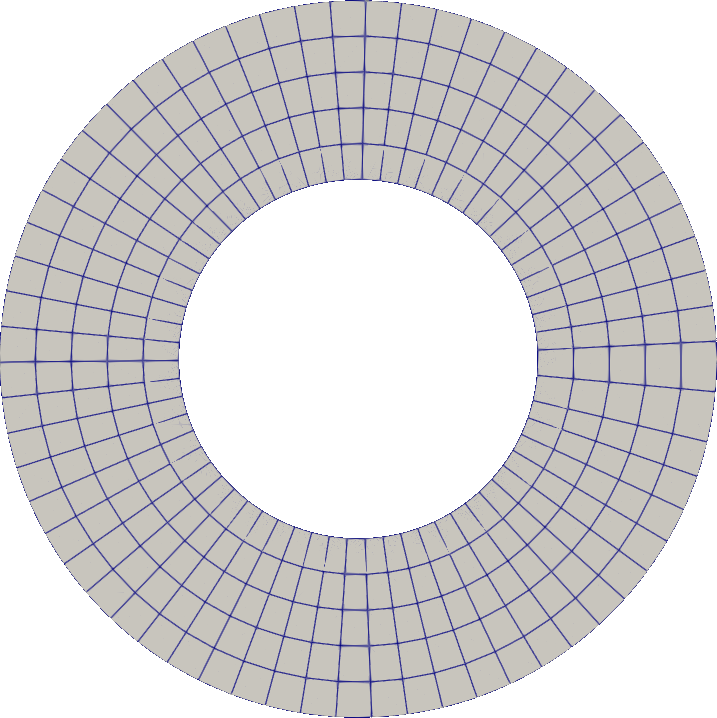
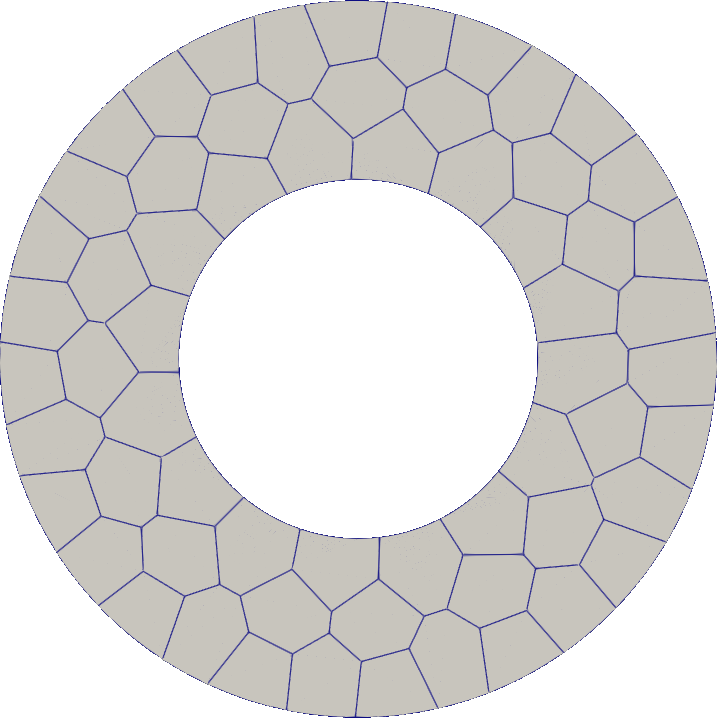
Figure 2: Computational domain for the example in section 4.1. On the left a representative of the first family quad of grids, made of radial rectangles. On the right a grid from the second family, composed by polygons and named poly.

We consider the following analytical solution

$$p_{\rm ex}(\bm{x},t)=\sin(0.5\pi t)\sin(0.5\pi{x}_{1}{x}_{2})(\|\bm{x}\|^{2}-r_{i}^{2})(\|\bm{x}\|^{2}-r_{o}^{2}),$$ (47)

together with Dirichlet conditions on the boundary and $\mu=1$, $\rho=1$. Source term and initial condition are computed accordingly to (47). We remark that solution is regular in space and time so that the hypothesis of Theorem 3.9 are verfied.

To consider only the space discretization error, we set $\Delta t=10^{-8}$ and compute the $H^{1}$ and $L^{2}$ errors in space at the end of the simulation time fiexd as $T=10\Delta t$.

Remark 4.1.

We notice that the asympotic behavoiur of the $H^{1}$-error can directly be inferred from the results of Theorem 3.9, while the $L^{2}$ error decay con be obtained by using similar arguments of those presented in [11]. The latter is beyond the scope of this work.

We consider two families of meshes: the first named quad is composed by radial rectangles while the second poly is constructed from a Voronoi tessellation, cf. Figure 2. In both cases the elements have curved edges at the boundary and straight internally. The errors in $L^{2}$ and semi-norm $H^{1}$ are computed as

$$L^{2}\text{ error}=\frac{\sqrt{\sum_{E\in\Omega_{h}}\|p_{\rm ex}-\Pi_{k}^{0}p\|_{E}^{2}}}{\|p_{\rm ex}\|_{\Omega_{h}}}\quad\text{and}\quad H^{1}\text{ error}=\frac{\sqrt{\sum_{E\in\Omega_{h}}\|\nabla p_{\rm ex}-\bm{\Pi}_{k-1}^{0}\nabla p\|_{E}^{2}}}{\|\nabla p_{\rm ex}\|_{\Omega_{h}}}.$$

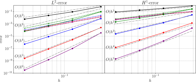
Figure 3: $L^{2}$ and $H^{1}$ error decay for the family quad in the example in Subsection 4.1.

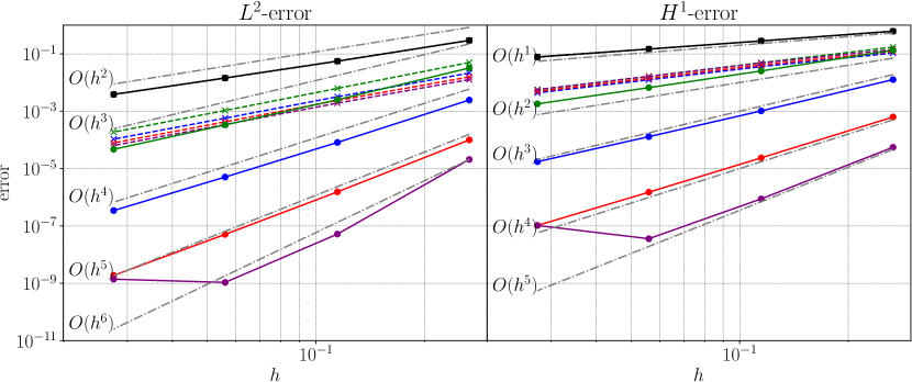
Figure 4: $L^{2}$ and $H^{1}$ error decay for the family poly in the example in Subsection 4.1.

Figure 3 shows the error decay for the family quad and Figure 4 for the family poly. In both cases we notice that for $k=1$ the $H^{1}$ error for withGeo and noGeo decays as expected, i.e., as $O(h^{k})$. However, for $k\geq 2$ the geometrical error dominates in the noGeo and limits the error decay to $O(h^{3/2})$. For the withGeo method the error decay behaves as expected reaching the convergence rate equal to $O(h^{k})$.

For the $L^{2}$-error the situation is similar, as we expect an error of convergence equal to $O(h^{k+1})$. As before, the geometrical error limits convergence rate for $k\geq 2$ for noGeo. Again, for the method withGeo the errors decay as expected. For degree $k=5$ in the poly we notice a stagnation of the error for small $h$ in both $L^{2}$ and $H^{1}$ norm, probably related to the numerical linear algebra. A numerical proof of this inference is that such phenomena is not present in the quad family. Indeed, quadrilateral meshes have more regular shapes with respect to the polygonal ones and, consequenly, the linear system arising from such discretization will have a lower condition number.

We can conclude that, at least for this example, the proposed method is an attractive approach to solve the wave equation with high order approximation in presence of curved boundaries.

4.2 Plane wave test case

In this second case, a plane wave enters the computational domain $\Omega=(-1,1)^{2}$ from the left boundary of and encounters a circular inclusion with different mechanical properties, i.e., a different $\mu$. The inclusion is a circle of radius 0.2, i.e.,

$$\gamma=\{\bm{x}:\|{\bm{x}}\|^{2}-0.2^{2}=0\}\,.$$

The computational domain is depicted in Figure 5. The computational grid is constructed starting from a Cartesian grid and then cutting all the elements that are crossed by $\gamma$. The obtained grid is not extremely refined around $\gamma$ since the exact geometry is captured by curved edges, indeed the number of elements is $6625$ compared to $6561$ of the original Cartesian grid. This fact represents an advantage from the computational point of view since we do not have to increase the number of degrees of freedom to capture the internal curved interface.

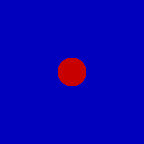
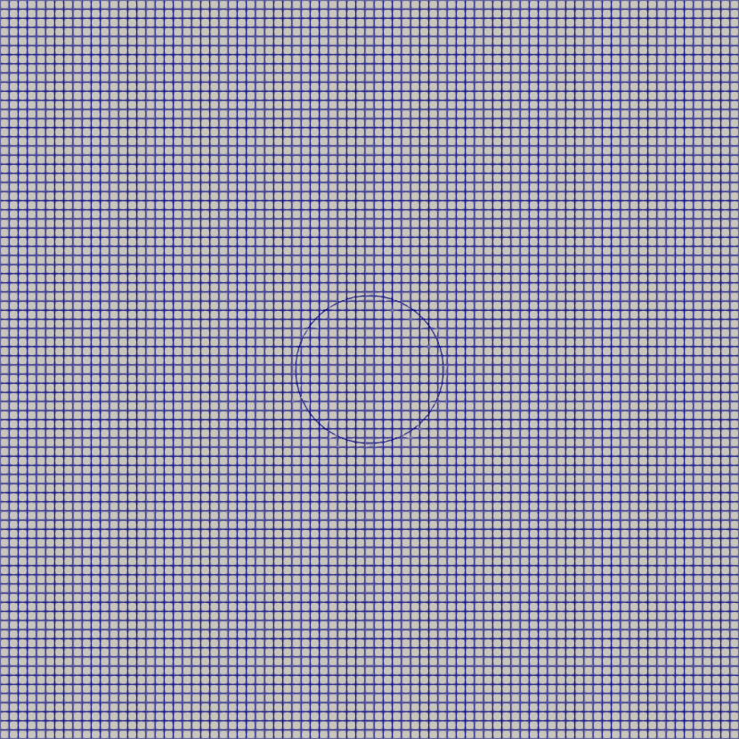
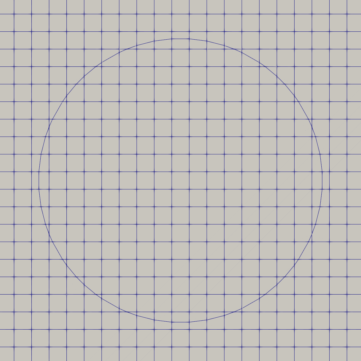
Figure 5: Computational domain for the example in section 4.1. On the left the domain with zone 1 and zone 2 highlighted. On the centre the computational grid, while on the right a zoom around the curved inclusion $\gamma$.

We solve Problem 2.3 where we set on the top and bottom edges a homogeneous Neumann condition, on the right edge an absorbing boundary condition, and on the left edge the following Dirichlet condition:

$$p(\bm{x},t)=\begin{dcases*}\sin({\color[rgb]{0,0,0}\omega}\pi t)&if $t\leq\frac{2}{{\color[rgb]{0,0,0}\omega}}$,\\ 0&otherwise,\end{dcases*}$$

being $\omega$ the angular frequency. The initial solution and velocity are set to zero, $\rho=1$, and the final time is set to $T=3$. In the blue region of Figure 5, outside the inclusion $\gamma$, we fix $\mu=1$ while in the red region, inside the inclusion, we chose $\mu=10^{-2}$. The source term $f$ is null, the approximation degree set to $k=4$ and the time step equal to $\Delta t=10^{-4}$.

We consider three different cases, depending on the wavelength $\lambda=\omega^{-1}$ and the dimension of the inclusion $\gamma$. In case (i) $\lambda=\frac{1}{2}$, so the resulting plane wave has a wavelength that is bigger than the dimension of $\gamma$. In case (ii), we set $\lambda=\frac{1}{5}$ which implies that the wavelength and the dimension of $\gamma$ are now comparable. Finally, in case (iii) the value of $\lambda$ is set to be $\lambda=\frac{1}{20}$. We obtain a plane wave with a wavelength that is much smaller than the dimension of $\gamma$. We want to understand, qualitatively, the impact of the curved geometry in our formulation for these cases.

The results are represented in Figure 6.

$p_{h}(\textbf{x},t)$
case (i)	case (ii)	case (iii)
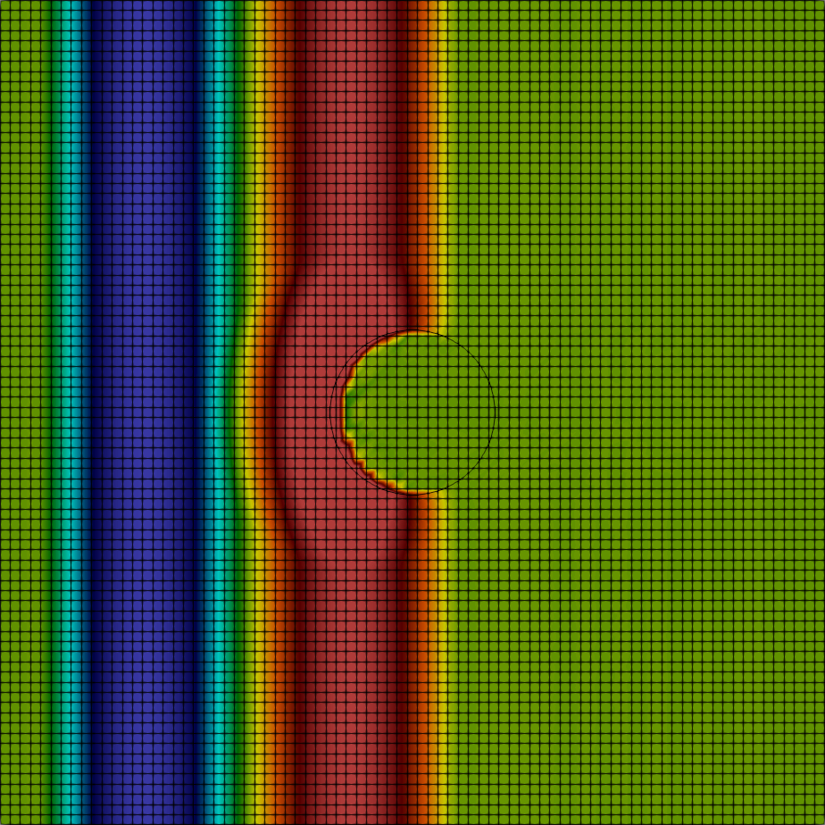
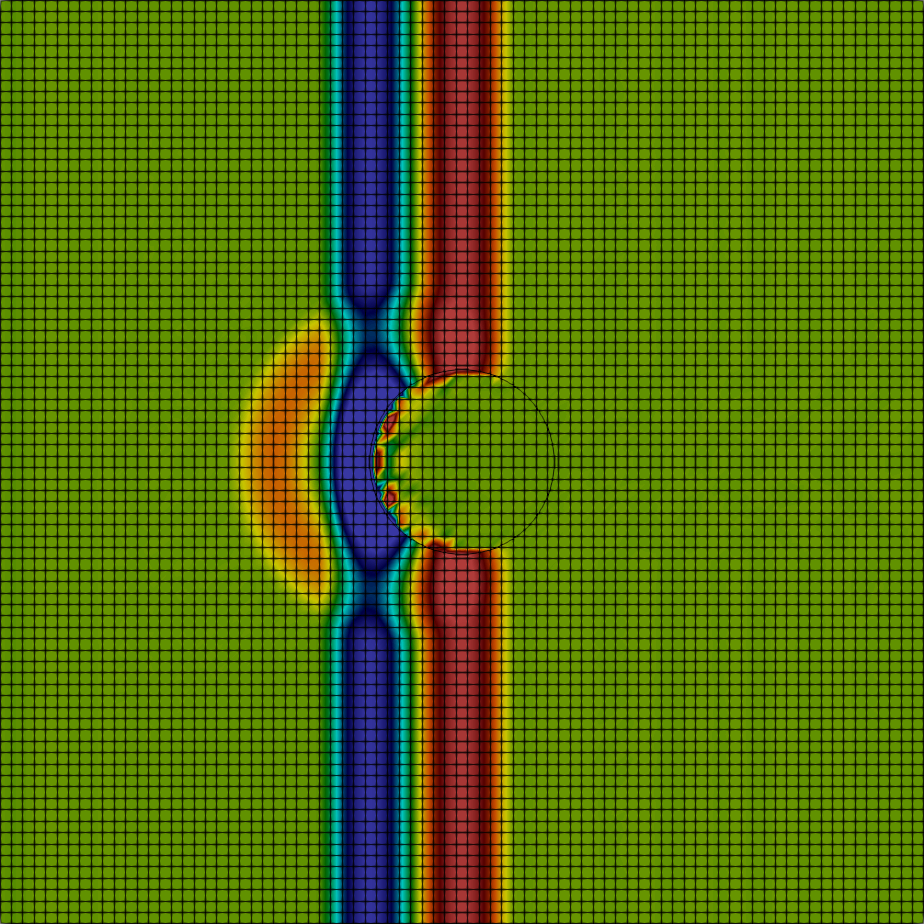
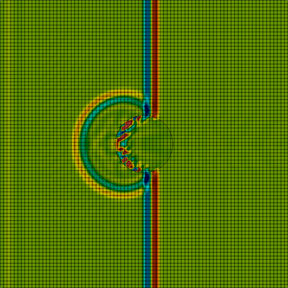
$t=6\Delta t$	$t=8\Delta t$	$t=10\Delta t$
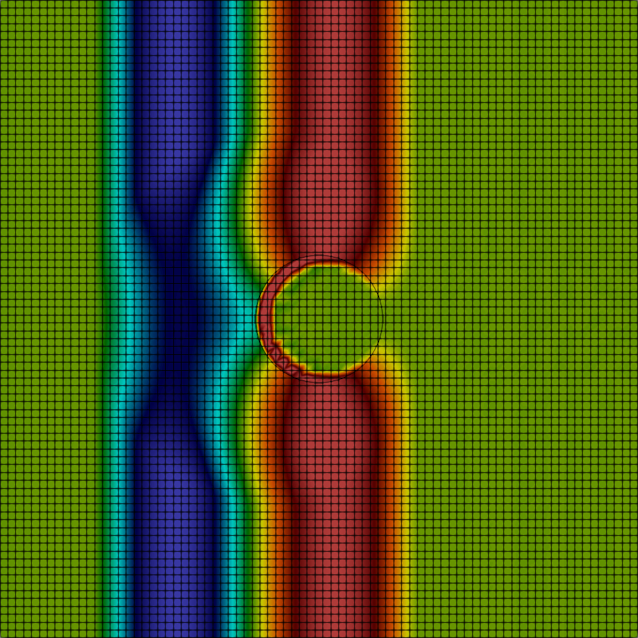
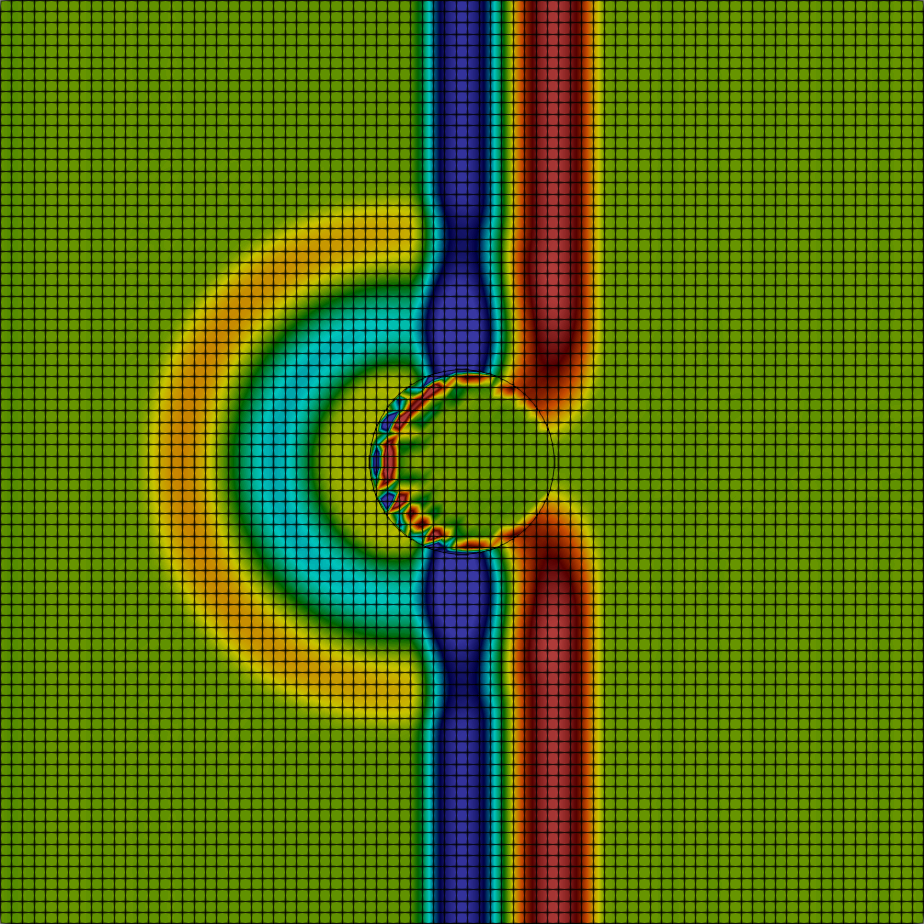
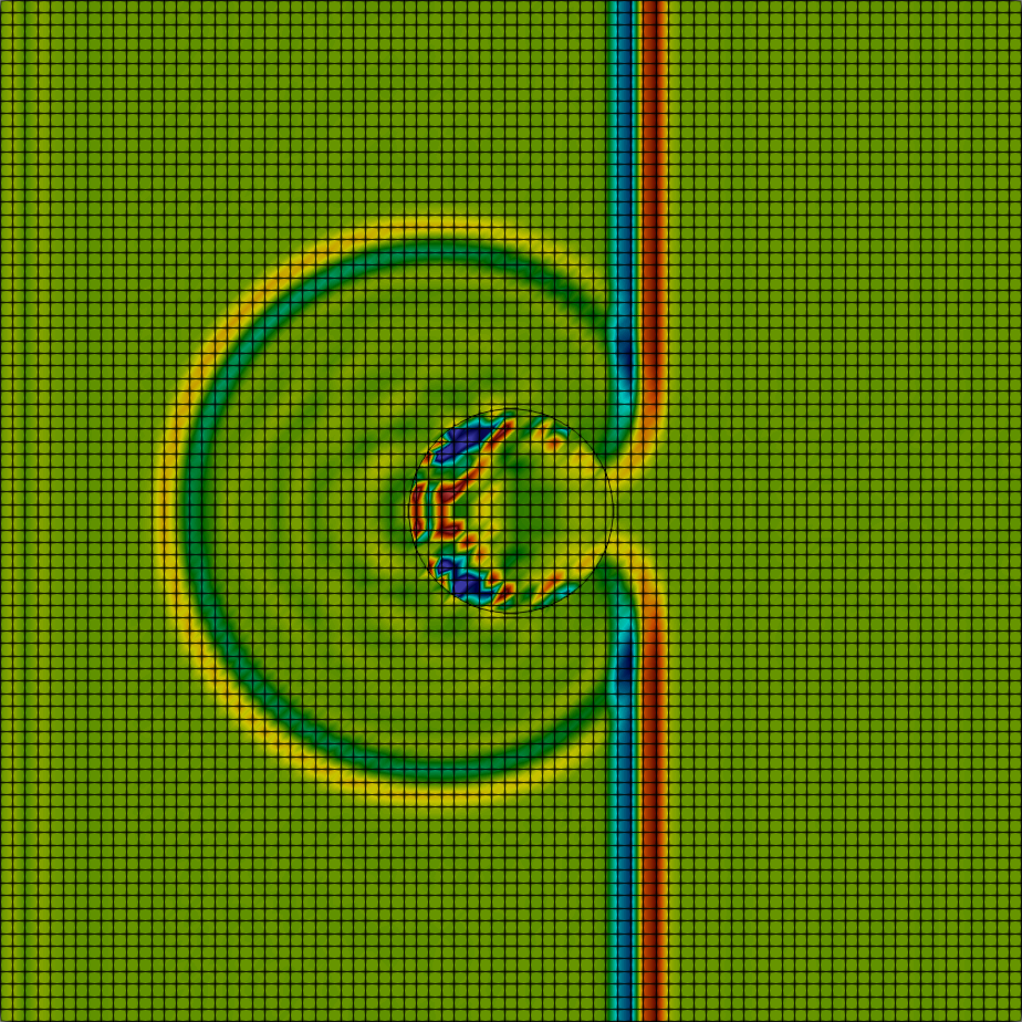
$t=6\Delta t$	$t=8\Delta t$	$t=10\Delta t$
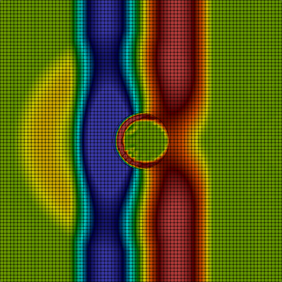
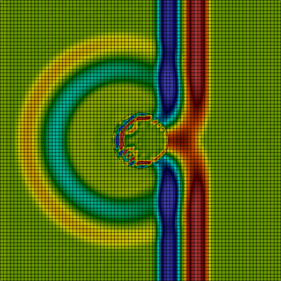
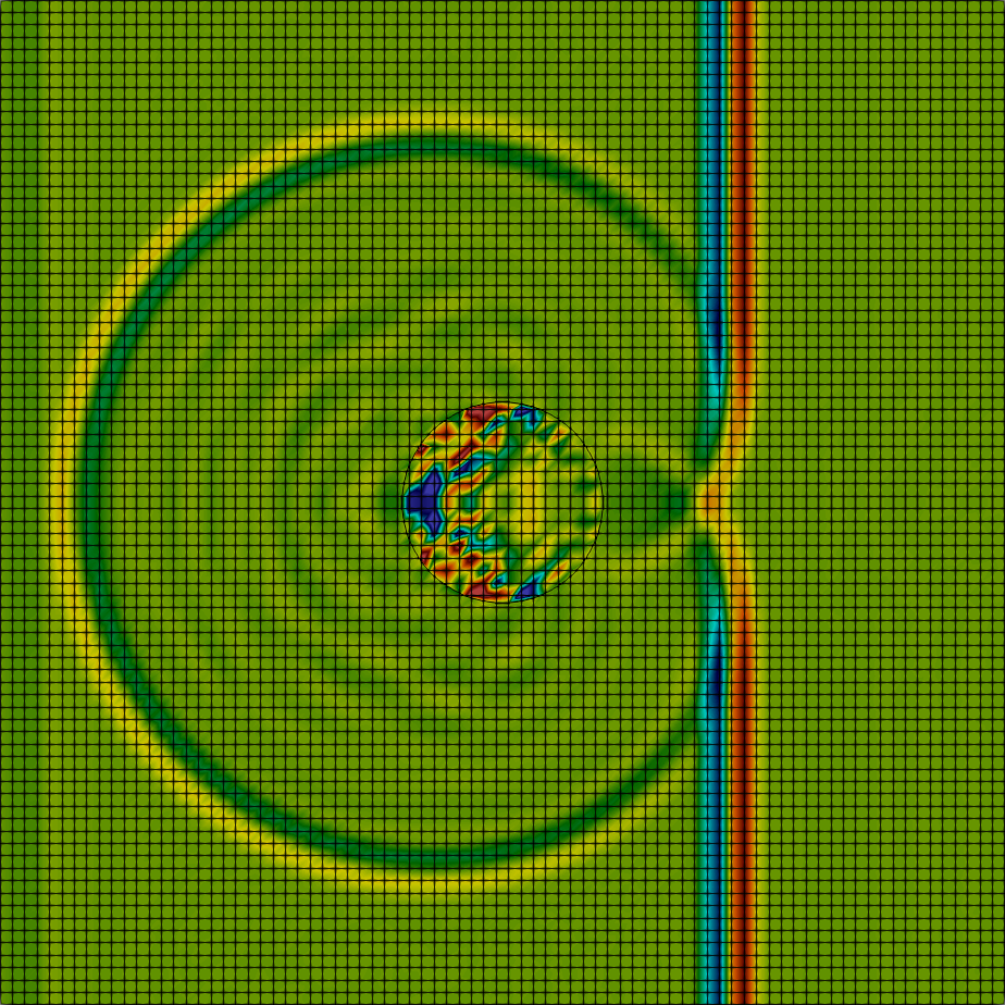
$t=6\Delta t$	$t=8\Delta t$	$t=10\Delta t$

Figure 6: Computed solution $p_{h}(\textbf{x},t)$ at three different time instants. Left: $\lambda=\frac{1}{2}$; center: $\lambda=\frac{1}{5}$ and right: $\lambda=\frac{1}{20}$.

The outcomes are, as expected, very different from each other. In case (i), when the wave encounters $\gamma$ we see the two phenomena of backward reflection of the wave and refraction inside $\gamma$. The latter is of small entity and the interior of $\gamma$ remains mostly unperturbed when $\lambda=\frac{1}{2}$. This latter phenomena is exacerbated by decreasing the value of $\lambda$, indeed for case (ii) we notice a more pronounced refraction effect inside $\gamma$ that becomes even more evident for case (iii). This phenomena are expected and confirm the quality of the obtained solution. No spurious oscillations due to the geometry (at least macroscopic ones) can be noticed in the reported plots.

We can conclude that, for this example, the proposed method is an attractive approach to solve the wave equation with high order approximation in presence of curved interfaces without the need of refining the computational grid nearby them.

4.3 Wave propagation with a realistic curved geometry

In this last test case, we consider a curved geometry that might represent a realistic case of a listric fault cutting a sequence of sedimentary layers. However, for the sake of simplicity, its dimensions are set as $\Omega=(-1,1)\times(-0.5,0.5)$, see Figure 7.

Figure 7: Computational domain for the example in section 4.3.

In the middle red areas are defined as $\Omega_{\rm mid}$. This central layer has different physical parameters than the surrounding portions of materials, see blue areas in Figure 7. Even if realistic applications with multiple layers are more challenging than this example, we show a qualitative analysis to understand the potentiality of the newly introduced method. Then, we consider Problem (2.1), with $\rho=1$ everywhere, $\mu=0.1$ in $\Omega_{\rm mid}$ and $\mu=1$ everywhere else. On all the boundaries we impose absorbing conditions, the initial data are null, the final time is $T=10$ and the source term is given as a Mexican-hat wavelet

$$f(\bm{x},t)=5[1-2\pi^{2}(t-1.2)^{2}]e^{-\pi^{2}(t-1.2)}e^{-\frac{(x_{0}+0.375)^{2}+(x_{1}-0.25)^{2}}{0.00625}}.$$

The geometry is obtained from a $32$ Cartesian grid where the curved elements are thus created by cutting the mesh with the curved interfaces. The resulting computational grid has 2271 elements. We consider a polynomial approximation order equal to $4$ and a time step $\Delta t=0.001$. The obtained numerical solution is depicted in Figure 8 for different time instants.

$p_{h}(\textbf{x},t)$
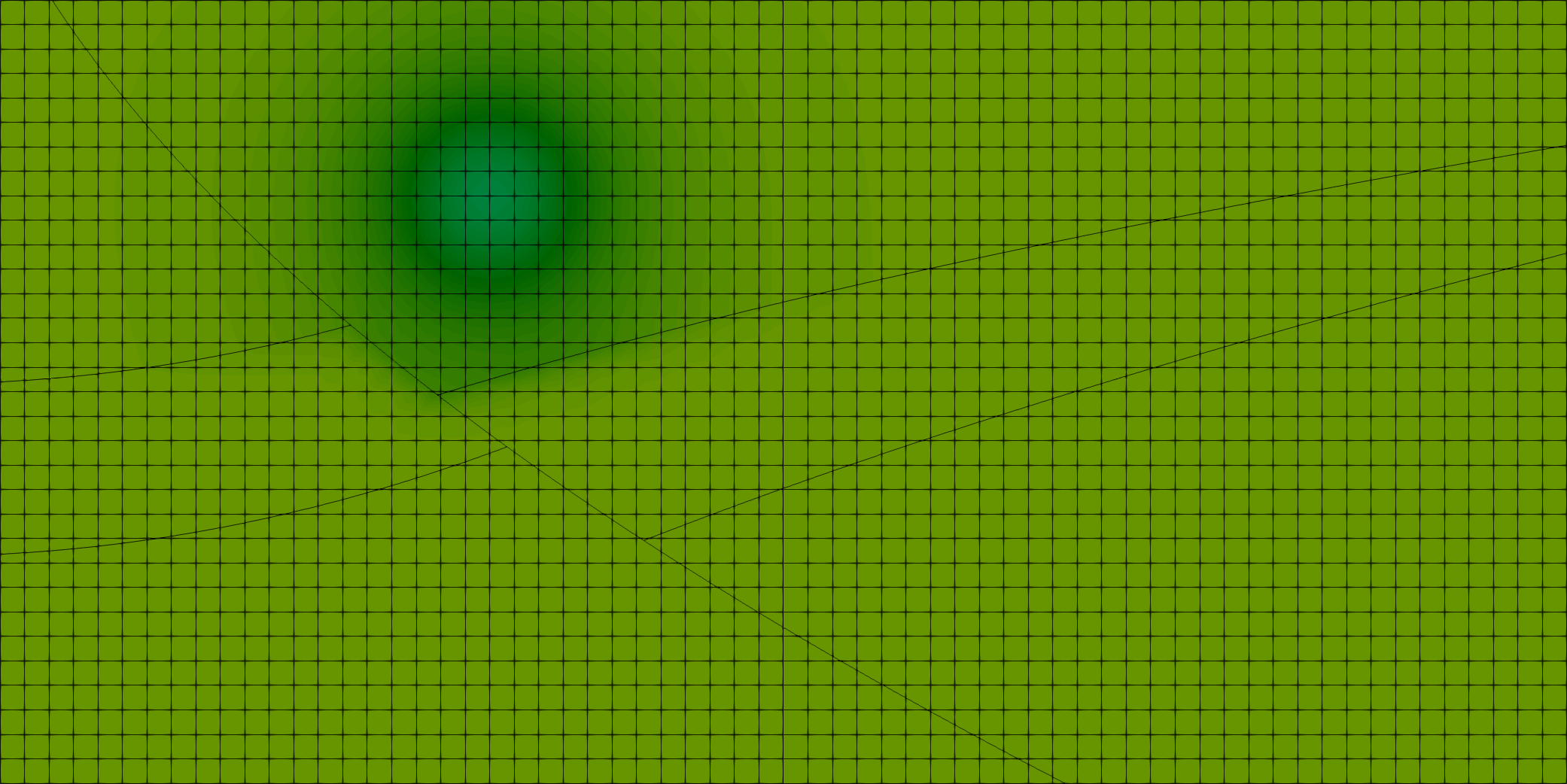
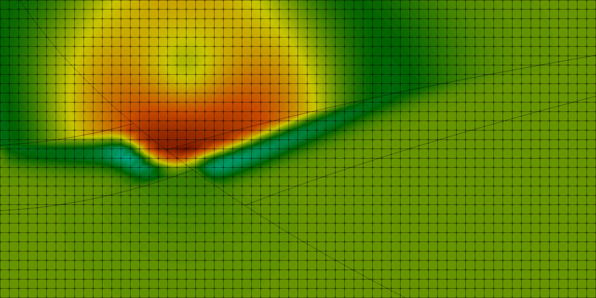
$t=\Delta t$	$t=5\Delta t$
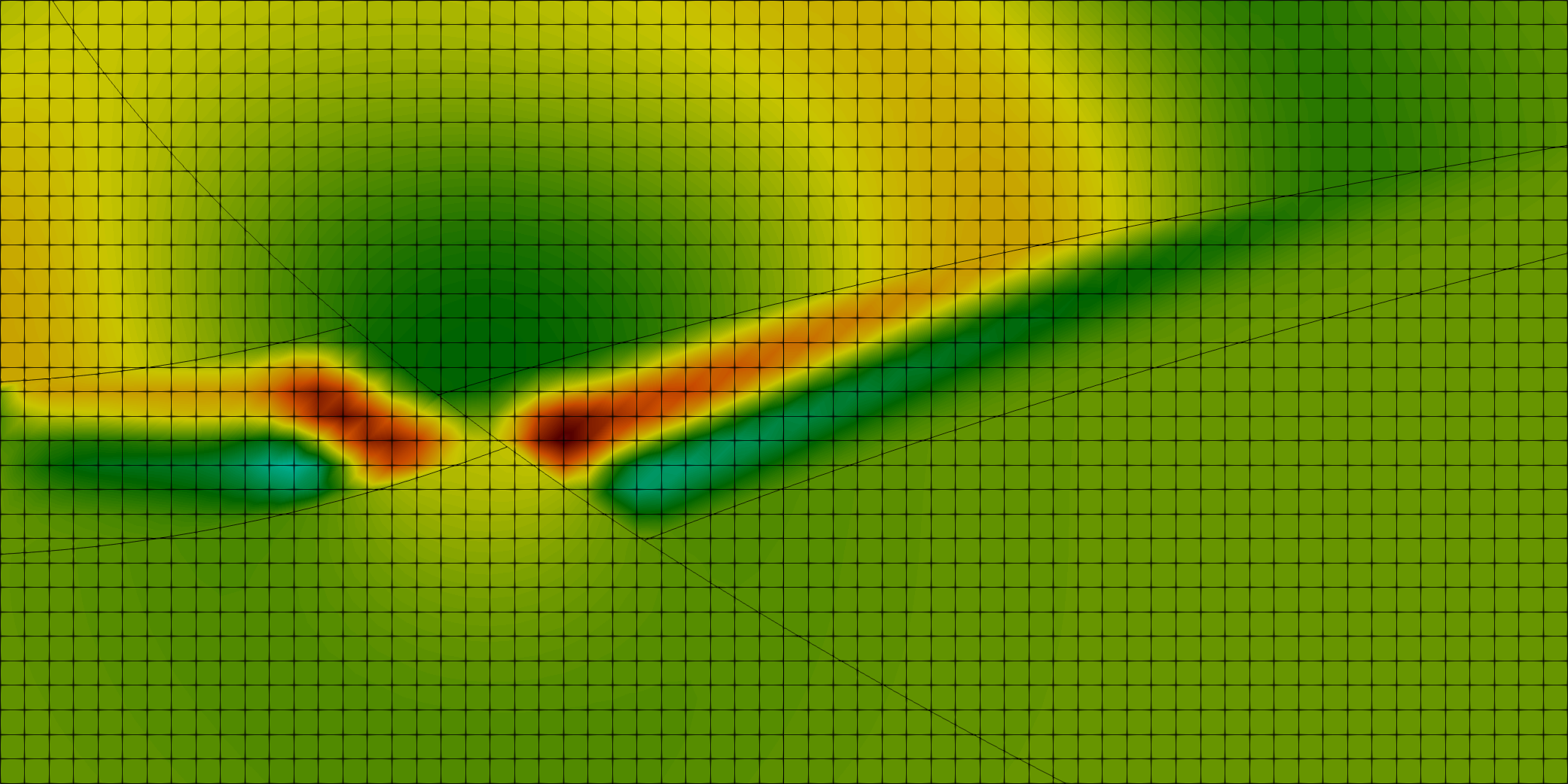
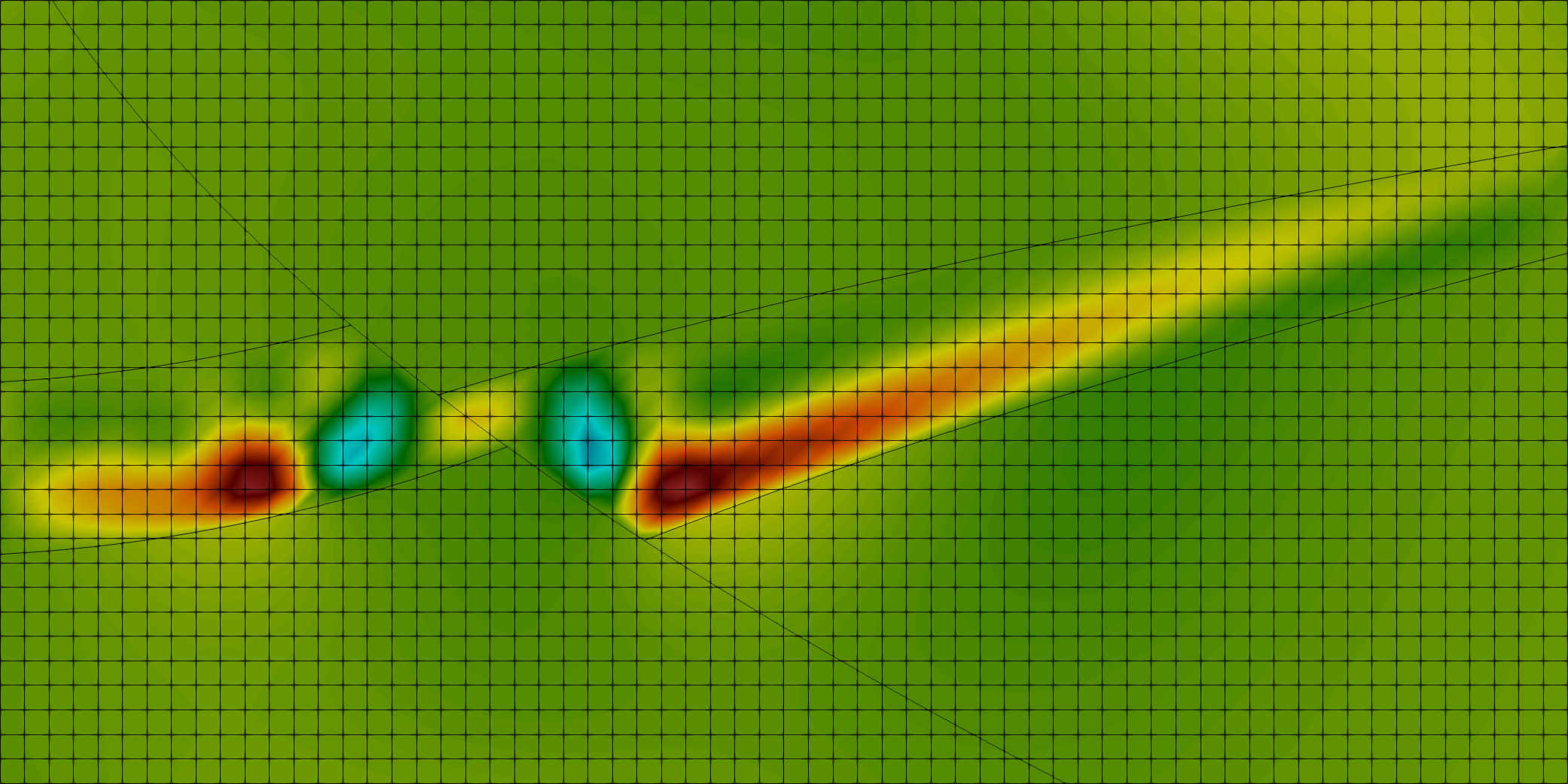
$t=7\Delta t$	$t=10\Delta t$
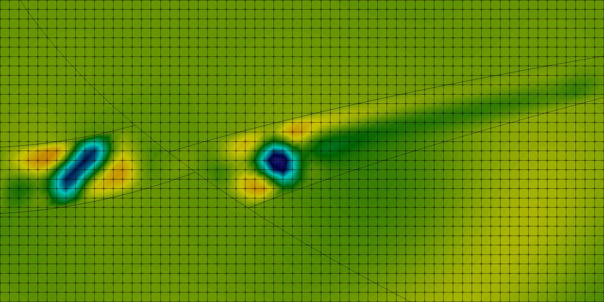
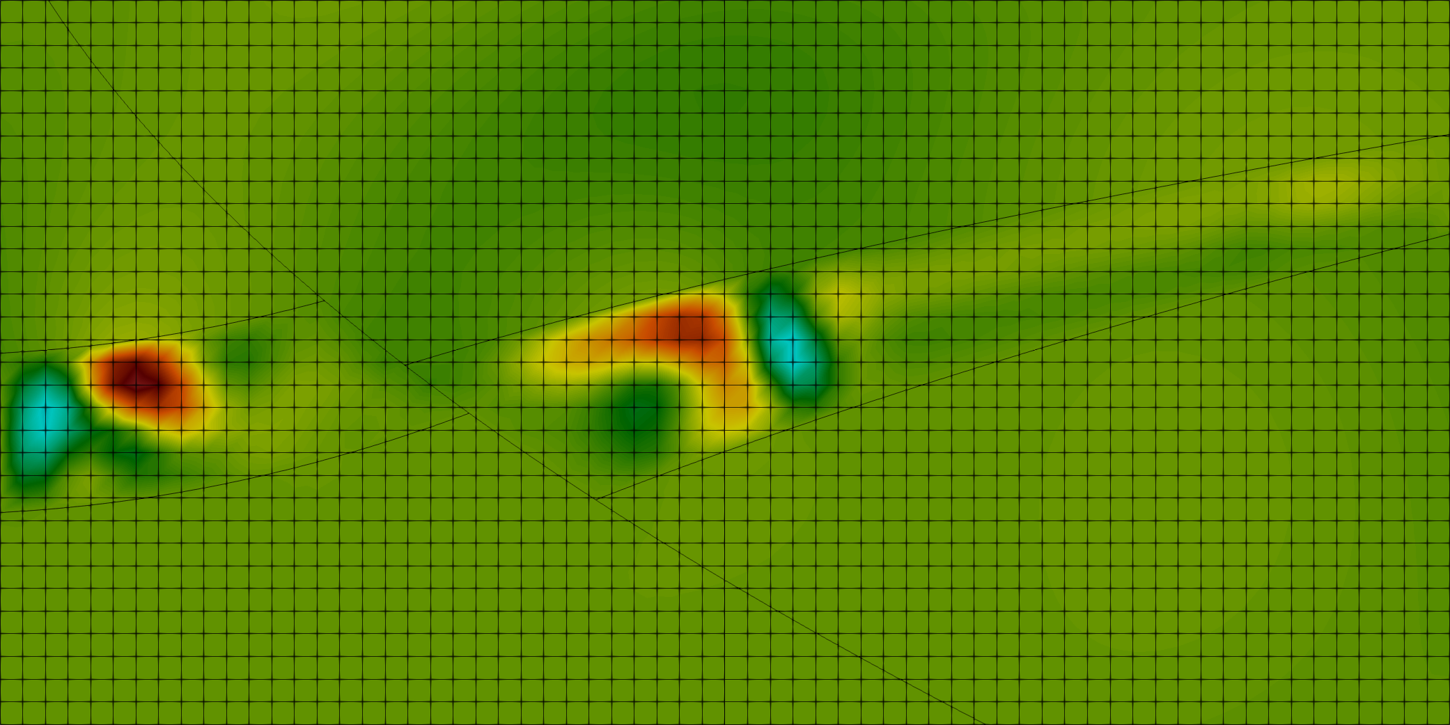
$t=14\Delta t$	$t=18\Delta t$
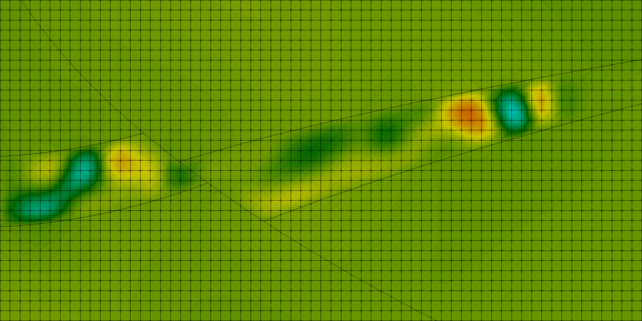
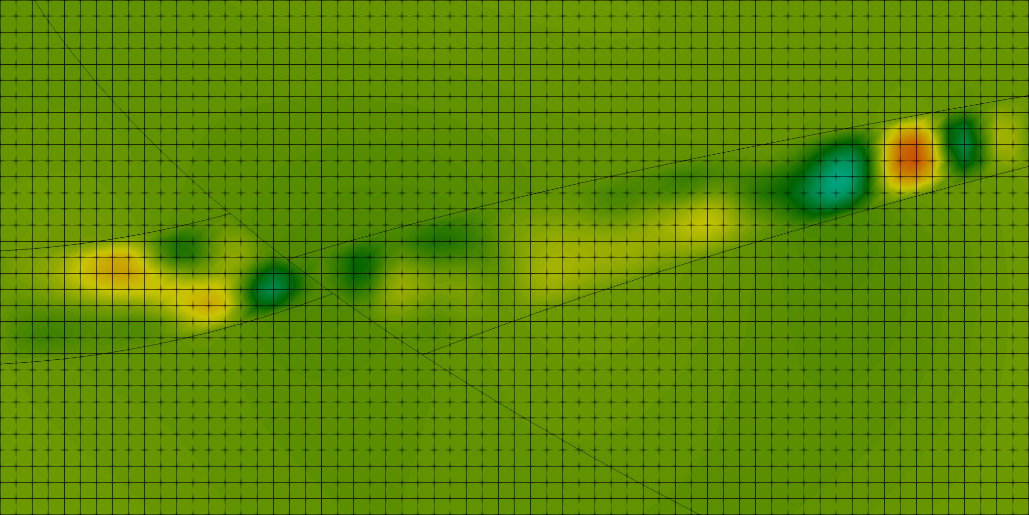
$t=34\Delta t$	$t=42\Delta t$

Figure 8: From left to right and from top to bottom, screenshots of the computed solution $p_{h}(\textbf{x},t)$ at different time instants.

From the obtained solution, we see that no spurious oscillations are generated at the curved interfaces inside the domain. Moreover, since the characteristic velocity in $\Omega_{\rm mid}$ is smaller than the surrounding parts, the wave remains trapped inside $\Omega_{\rm mid}$.

Also in this final test case, even on a more complex curved geometry, the proposed scheme performs well, without any need to over-refine around the curved interfaces to avoid side effects.

5 Conclusions

In this paper, we have extended the Virtual Element Method in primal form for the wave equation when the computational domain has internal curved interfaces and/or curved boundaries. The latter are represented exactly in order to avoid possible geometrical errors that might affect the quality of the numerical solution and limit the convergence order. This preliminary study carried out in a two-dimensional setting and the promising results shown, open the possibility to extend the proposed approach to more complex three dimensional configurations. The numerical examples presented testify that this approach is very effective, since no spurious oscillations due to curved geometries arise. Moreover, it gives the possibility to handle the geometrical challenges arising in realistic applications.

Aknowledgements

The authors are members of the INdAM Research group GNCS and this work is partially funded by INdAM-GNCS through the project “Bend VEM 3d”.

References

- [1] J. Aghili, D. A. Di Pietro, and B. Ruffini. An -hybrid high-order method for variable diffusion on general meshes. Comput. Methods Appl. Math., 17(3):359–376, 2017.
- [2] B. Ahmad, A. Alsaedi, F. Brezzi, L. D. Marini, and A. Russo. Equivalent projectors for virtual element methods. Comput. Math. Appl., 66(3):376–391, 2013.
- [3] P. F. Antonietti, L. Beirão da Veiga, N. Bigoni, and M. Verani. Mimetic finite differences for nonlinear and control problems. Math. Models Methods Appl. Sci., 24(8):1457–1493, 2014.
- [4] P. F. Antonietti, F. Bonaldi, and I. Mazzieri. A high-order discontinuous Galerkin approach to the elasto-acoustic problem. Comput. Methods Appl. Mech. Engrg., 358:112634, 29, 2020.
- [5] P. F. Antonietti, A. Cangiani, J. Collis, Z. Dong, E. H. Georgoulis, S. Giani, and P. Houston. Review of Discontinuous Galerkin Finite Element Methods for Partial Differential Equations on Complicated Domains. Lect. Notes Comput. Sci. Eng., 114:281 – 310, 2015.
- [6] P. F. Antonietti, L. B. da Veiga, D. Mora, and M. Verani. A stream Virtual Element formulation of the Stokes problem on polygonal meshes. SIAM J. Numer. Anal., 52(1):386–404, 2014.
- [7] P. F. Antonietti, L. B. da Veiga, S. Scacchi, and M. Verani. A Virtual Element Method for the Cahn-Hilliard equation with polygonal meshes. SIAM J. Numer. Anal., 54(1):34–56, 2016.
- [8] P. F. Antonietti, L. Formaggia, A. Scotti, M. Verani, and N. Verzotti. Mimetic finite difference approximation of flows in fractured porous media. M2AN Math. Model. Numer. Anal., 50(3):809–832, 2016.
- [9] P. F. Antonietti, P. Houston, X. Hu, M. Sarti, and M. Verani. Multigrid algorithms for hp-version interior penalty discontinuous Galerkin methods on polygonal and polyhedral meshes. Calcolo, 54(4):1169–1198, 2017.
- [10] P. F. Antonietti, P. Houston, and G. Pennesi. Fast numerical integration on polytopic meshes with applications to discontinuous Galerkin finite element methods. J. Sci. Comput., 77:1339–1370, 2018.
- [11] P. F. Antonietti, G. Manzini, I. Mazzieri, H. M. Mourad, and M. Verani. The arbitrary-order virtual element method for linear elastodynamics models: convergence, stability and dispersion-dissipation analysis. Internat. J. Numer. Methods Engrg., 122(4):934–971, 2021.
- [12] P. F. Antonietti, G. Manzini, and M. Verani. The fully nonconforming Virtual Element Method for biharmonic problems. Math. Models Methods Appl. Sci., 28(02):387–407, 2018. M3AS Math. Models Methods Appl. Sci., to appear.
- [13] P. F. Antonietti and I. Mazzieri. High-order Discontinuous Galerkin methods for the elastodynamics equation on polygonal and polyhedral meshes. Comput. Methods Appl. Mech. Engrg., 342:414–437, 2018.
- [14] P. F. Antonietti, I. Mazzieri, M. Muhr, V. Nikolić, and B. Wohlmuth. A high-order discontinuous Galerkin method for nonlinear sound waves. Journal of Computational Physics, 415:109484, 2020.
- [15] E. Artioli, L. Beirão da Veiga, and F. Dassi. Curvilinear Virtual Elements for 2D solid mechanics applications. Comput. Methods Appl. Mech. Engrg., 359:112667, 2020.
- [16] B. Ayuso de Dios, K. Lipnikov, and G. Manzini. The nonconforming Virtual Element Method. ESAIM Math. Model. Numer. Anal., 50(3):879 – 904, 2016.
- [17] L. Beirão da Veiga, F. Brezzi, A. Cangiani, G. Manzini, L. D. Marini, and A. Russo. Basic principles of Virtual Element Methods. Math. Models Methods Appl. Sci., 23(1):199 – 214, 2013.
- [18] L. Beirão da Veiga, F. Brezzi, F. Dassi, L. D. Marini, and A. Russo. A family of three-dimensional virtual elements with applications to magnetostatics. SIAM J. Numer. Anal., 56(5):2940–2962, 2018.
- [19] L. Beirão da Veiga, F. Brezzi, L. D. Marini, and A. Russo. The Hitchhiker’s guide to the virtual element method. Mathematical Models and Methods in Applied Sciences, 24(08):1541–1573, 2014.
- [20] L. Beirão da Veiga, F. Brezzi, L. D. Marini, and A. Russo. Polynomial preserving virtual elements with curved edges. Math. Models Methods Appl. Sci., 30(8):1555–1590, 2020.
- [21] L. Beirão da Veiga, F. Dassi, and A. Russo. High-order virtual element method on polyhedral meshes. Comput. Math. Appl., 74(5):1110–1122, 2017.
- [22] L. Beirão da Veiga, K. Lipnikov, and G. Manzini. The Mimetic Finite Difference method for elliptic problems, volume 11. Springer, Cham, 2014.
- [23] L. Beirão da Veiga, D. Mora, and G. Vacca. The Stokes complex for virtual elements with application to Navier-Stokes flows. J. Sci. Comput., 81(2):990–1018, 2019.
- [24] L. Beirão da Veiga, A. Russo, and G. Vacca. The virtual element method with curved edges. ESAIM Math. Model. Numer. Anal., 53(2):375–404, 2019.
- [25] L. Beirão da Veiga, F. Brezzi, L. Marini, and A. Russo. Virtual Element Method for general second-order elliptic problems on polygonal meshes. Math. Models Methods Appl. Sci., 26(04):729–750, 2016.
- [26] M. F. Benedetto, S. Berrone, S. Pieraccini, and S. Scialò. The virtual element method for discrete fracture network simulations. Comput. Methods Appl. Mech. Engrg., 280:135–156, 2014.
- [27] S. Bertoluzza, M. Pennacchio, and D. Prada. High order VEM on curved domains. Atti Accad. Naz. Lincei Rend. Lincei Mat. Appl., 30(2):391–412, 2019.
- [28] L. Botti and D. A. Di Pietro. Assessment of hybrid high-order methods on curved meshes and comparison with discontinuous Galerkin methods. J. Comput. Phys., 370:58–84, 2018.
- [29] M. Botti, D. A. Di Pietro, and P. Sochala. A hybrid high-order method for nonlinear elasticity. SIAM J. Numer. Anal., 55(6):2687–2717, 2017.
- [30] S. C. Brenner and L. R. Scott. The Mathematical Theory of Finite Element Methods, volume 15 of Texts in Applied Mathematics. Springer, New York, third edition, 2008.
- [31] H. Brezis. Operateurs maximaux monotones et semi-groupes de contractions dans les espaces de Hilbert. Number 5 in Mathematical Studies. North-Holland Publishing Company, Amsterdam, 1973.
- [32] F. Brezzi, K. Lipnikov, and M. Shashkov. Convergence of Mimetic Finite Difference method for diffusion problems on polyhedral meshes with curved faces. Math. Models Methods Appl. Sci., 16(2):275–297, 2006.
- [33] F. Brezzi, K. Lipnikov, and V. Simoncini. A family of Mimetic Finite Difference methods on polygonal and polyhedral meshes. Math. Models Methods Appl. Sci., 15(10):1533–1551, 2005.
- [34] E. Burman, M. Cicuttin, G. Delay, and E. A. An unfitted hybrid high-order method with cell agglomeration for elliptic interface problems. SIAM J. Sci. Comput., 43(2):A859–A882, 2021.
- [35] A. Cangiani, Z. Dong, E. H. Georgoulis, and P. Houston. -version discontinuous Galerkin methods on polytopic meshes. SpringerBriefs in Mathematics. Springer International Publishing, 2017.
- [36] A. Cangiani, E. H. Georgoulis, T. Prayer, and O. J. Sutton. A posteriori error estimates for the virtual element method. Numer. Math., 137:857––893, 2017.
- [37] A. Cangiani, G. Manzini, and O. J. Sutton. Conforming and nonconforming Virtual Element Methods for elliptic problems. IMA J. Numer. Anal., 37(3):1317–1354, 2017.
- [38] F. Chave, D. A. Di Pietro, and L. Formaggia. A hybrid high-order method for Darcy flows in fractured porous media. SIAM J. Sci. Comput., 40(2):A1063–A1094, 2018.
- [39] J. A. Cottrell, T. J. R. Hughes, and Y. Bazilevs. Isogeometric analysis: toward integration of CAD and FEA. John Wiley & Sons, 2009.
- [40] F. Dassi, A. Fumagalli, D. Losapio, S. Scialò, A. Scotti, and G. Vacca. The mixed virtual element method on curved edges in two dimensions. submitted to CMAME, arXiv:2007.13513, 2020.
- [41] J. D. De Basabe and M. K. Sen. A comparison of finite-difference and spectral-element methods for elastic wave propagation in media with a fluid-solid interface. Geophys. J. Int., 200:278–298, 2015.
- [42] D. A. Di Pietro and A. Ern. Hybrid high-order methods for variable-diffusion problems on general meshes. C. R. Math. Acad. Sci. Paris, 353(1):31–34, 2015.
- [43] D. A. Di Pietro and S. Krell. A hybrid high-order method for the steady incompressible Navier-Stokes problem. J. Sci. Comput., 74(3):1677–1705, 2018.
- [44] J. Droniou, R. Eymard, and R. Herbin. Gradient schemes: generic tools for the numerical analysis of diffusion equations. ESAIM Math. Model. Numer. Anal., 50(3):749–781, 2016.
- [45] G. Duvant and J. Lions. Inequalities in Mechanics and Physics, volume 219 of Grundlehren der mathematischen Wissenschaften. Springer-Verlag Berlin Heidelberg, Berlin, 1976.
- [46] M. J. Gander and L. Halpern. Absorbing boundary conditions for the wave equation and parallel computing. Math. Comp., 74(249):153–176, 2005.
- [47] M. Grote, A. Schneebeli, and D. Schötzau. Discontinuous Galerkin finite element method for the wave equation. SIAM J. Numer. Anal., 44(6):2408–2431, 2006.
- [48] M. Käser and M. Dumbser. A highly accurate discontinuous Galerkin method for complex interfaces between solids and moving fluids. Geophysics, 73:T23–T35, 2008.
- [49] D. Komatitsch, C. Barnes, and J. Tromp. Wave propagation near a fluid‐solid interface: A spectral‐element approach. Geophysics, 65(2):623–631, 2000.
- [50] M. Lenoir. Optimal isoparametric finite elements and error estimates for domains involving curved boundaries. SIAM J. Numer. Anal., 23(3):562–580, 1986.
- [51] F. Müller, D. Schötzau, and C. Schwab. Discontinuous Galerkin methods for acoustic wave propagation in polygons. J. Sci. Comp., 3(01):1909–1935, 2018.
- [52] B. Rivière and M. F. Wheeler. Discontinuous finite element methods for acoustic and elastic wave problems. Contemporary Mathematics, 329:271–282, 2003.
- [53] G. Seriani. A parallel spectral element method for acoustic wave modeling. J. Comput. Acoust., 05(01):53–69, 1997.
- [54] S. Terrana, J. P. Vilotte, and L. Guillot. A spectral hybridizable discontinuous Galerkin method for elastic–acoustic wave propagation. Geophys. J. Int., 213:574–602, 2018.
- [55] L. C. Wilcox, G. Stadler, C. Burstedde, and O. Ghattas. A high-order discontinuous Galerkin method for wave propagation through coupled elastic-acoustic media. J. Comput. Phys., 229:9373–9396, 2010.
- [56] E. Zampieri and L. F. Pavarino. Implicit spectral element methods and Neumann–Neumann preconditioners for acoustic waves. Comput. Methods Appl. Mech. Engrg., 195(19):2649 – 2673, 2006.