Losses in interacting quantum gases: ultra-violet divergence and its regularization

Abstract

We investigate the effect of losses on an interacting quantum gas. We show that, for gases in dimension higher than one, assuming together a vanishing correlation time of the reservoir where dissipation occurs, and contact interactions leads to a divergence of the energy increase rate. This divergence is a combined effect of the contact interactions, which impart arbitrary large momenta to the atoms, and the infinite energy width of the reservoir associated to its vanishing correlation time. We show how the divergence is regularized when taking into account the finite energy width of the reservoir, and, for large energy width, we give an expression for the energy increase rate that involves the contact parameter. We then consider the specific case of a weakly interacting Bose Einstein condensate, that we describe using the Bogoliubov theory. Assuming slow losses so that the gas is at any time described by a thermal equilibrium, we compute the time evolution of the temperature of the gas. Using a Bogoliubov analysis, we also consider the case where the regularization of the divergence is due to the finite range of the interaction between atoms.

The effect of the coupling of a many-body quantum system to an environment attracted a lot of attention in the last years, in the context of cold atoms experiments. Engineered coupling was proposed to realize particular many-body states Diehl et al. (2008); Poletti et al. (2013), including strongly correlated phases or highly entangled states Barreiro et al. (2011). It can also be used as a resource for quantum computation Verstraete et al. (2009). A particular coupling to an environment, that has received a lot of attention recently, is realized when the gas suffers from losses. Losses can produce highly correlated phases Roncaglia et al. (2010); Kantian et al. (2009); Foss-Feig et al. (2012); Syassen et al. (2008), induce Zenon effect Barontini et al. (2013); Nakagawa et al. (2021); García-Ripoll et al. (2009), drive phase transition Labouvie et al. (2016), lead to non-thermal states Johnson et al. (2017); Bouchoule et al. (2020); Rossini et al. (2020); Bouchoule and Dubail (2021), and produce cooling Rauer et al. (2016); Schemmer and Bouchoule (2018); Bouchoule and Schemmer (2020). In all the works mentioned above, the coupling to the environment is described assuming that the correlation time of the environment is much smaller than any characteristic evolution time of the system. Then the time evolution of the system obeys a universal Lindblad equation (see the review Daley (2014)) describing the coupling to an environment of vanishing correlation time. In this paper we show that this approximation is not always correct.

For a homogeneous single atom loss process, the universal Lindblad equation reads, for a gas in the continuous space,

$$\frac{d\rho}{dt}=-(i/\hbar)[H_{0},\rho]+\Gamma\int d^{d}{\bf r}\left\{-\frac{1}{2}\{\psi^{+}_{\bf r}\psi_{\bf r},\rho\}+\psi_{\bf r}\rho\psi^{+}_{\bf r}\right\}$$ (1)

where $H_{0}$ is the Hamiltonian of the quantum gas, $\rho$ is its density matrix, $d$ is the dimension of system, $\psi_{r}$ annihilates an atom at position ${\bf r}$, and $\Gamma$ is the loss rate. For simplicity we consider here a single specy gas. Eq. (1) is universal in the sense that the loss process is characterized by a single parameter $\Gamma$, details of the reservoir being irrelevant.

The evolution under the above Lindblad equation is simple if one assumes the state of the gas is uncorrelated, for instance within a mean-field approximation : the population of each single particle state decreases exponentially  Barontini et al. (2013). However, interactions between atoms introduce correlations, which highly complicates the calculation of the effect of losses. In cold atoms experiments, the range of the interaction potential between atoms is typically much smaller than all length scales in the problem. Then the effect of interactions is well modeled by a contact interaction term. This description of interactions is also a universal model: details of the interaction potential is irrelevant and interactions are described by a single parameter, the scattering length. In this paper, we show that the combination of the two above universal models leads to unphysical predictions in dimensions higher than one: for a gas with contact interaction evolving under Eq. (1), the increase rate of the energy diverges.

The divergence of the energy increase rate originates from the following process. The contact interaction in the gas is responsible for singularities of the many body wavefunction when two atoms meet Werner and Castin (2012a), leading, in dimension higher than one, to a diverging kinetic energy, this divergence being counterbalanced by the interaction energy such that the total energy is finite. The Lindlab dynamics of Eq. (1) assumes that loss events are instantaneous with respect with the gas dynamics: within the quantum trajectory description equivalent to the Lindblad dynamics Daley (2014) a loss event corresponds to the instantaneous action of the jump operator $\psi_{\bf r}$. Thus, just after a loss event occurred, the many-body wavefunction of the remaining atoms is equal to its value just before the loss event. This wave function presents a singularity when the position of an atom approaches the position of the lost atom. The divergence of the kinetic energy associated with this singularity, is no longer counterbalanced by interaction energy: it amounts to an infinite value of the energy in the system. Note that the infinitely large increase of the energy is made possible by the infinite energy available in the reservoir involved in the loss process: the vanishing correlation time is associated to an infinite energy width.

Several mechanisms could lead to a regularization of the above divergence. First, the finite range of the interaction between the atoms will introduce a cutoff that prevents the divergence of the kinetic energy. Second, the reservoir has in practice a finite energy width which limits the maximum energy a loss event can deposit in the system. In this paper, we consider both regularizations, with an emphasis on the effect of the finite reservoir energy-width.

We first propose a model for the loss mechanism, with a finite energy width $E_{\rm res}$. Using an analysis of the 2-atoms case, we then derive the expected value of the energy density increase rate for a gas with contact interactions, valid for large $E_{\rm res}$. We find a general expression, that involves the contact parameter. Although our derivation concentrates on the Bosonic case for simplicity of notations, our results are general. To compute the evolution of the system beyond this limit of large $E_{\rm res}$, one needs a many-body model of the system that includes correlations between atoms introduced by interactions. We will concentrate on the case of a weakly interacting Bose-Einstein condensate and we use the Bogoliubov description. Within this framework, we compute the evolution of the energy. Assuming a loss rate much smaller than the relaxation rate of the gas, the system can be described locally at any time by a thermal equilibrium state. We compute the expected evolution of the temperature under the effect of losses. Within the Bogoliubov treatment, we also consider the case where the regularization comes from the finite range of the interactions.

Model for the loss process.

We consider a gas made of particles of mass $m$ in dimension $d=1$ (1D), $d=2$ (2D) or $d=3$ (3D), and we use periodic boundary conditions in a box of size $L^{d}$. A homogeneous one-body loss process occurs if, at each point, the atoms are coupled to a continuum. In a gas confined in 1D or 2D, the frozen dimension(s) could serve as the continuum, if atoms are coupled to an untrapped state. In 3D, the loss mechanism could be the de-excitation of the atoms, if the latter are in a metastable state, in which case the momentum of the emitted photon provides the continuum for the loss mechanism. Here instead we will consider a simpler, yet equivalent model SM , where the loss mechanism is induced by a noisy coupling to an untrapped internal state, the different Fourier components playing the role of the continuum. This would correspond to the effect of a noisy magnetic field for magnetically trapped atoms Bouchoule and Schemmer (2020). More precisely, we consider a coupling to the reservoir which writes

$$V=\int d^{d}{\bf r}\Omega(t)\psi_{\bf r}b^{+}_{\bf r}+\,h.c.=\sum_{\bf p}\Omega(t)\Psi_{\bf p}B^{+}_{\bf p}\,+h.c.,$$ (2)

where $\psi_{\bf r}$, resp. $b_{\bf r}$, annihilates an atom of the system, resp. of the reservoir, at position ${\bf r}$, $\Psi_{\bf p}$, resp. $B_{\bf p}$, annihilates an atom of the system, resp. of the reservoir, of momentum ${\bf p}$, $h.c.$ is the abbreviation of “hermitian conjugate” and ${\Omega}(t)$ is a noisy function. ${\bf p}$ takes discrete values whose coordinates are multiple of $2\pi\hbar/L$, and we note $p=|{\bf p}|$. We define the energy-dependent rate $\Gamma(E)$ from the spectral density of $\Omega(t)$ according to

$$\Gamma(E)=\frac{1}{\hbar^{2}}\int d\tau e^{-iE\tau/\hbar}\langle{\Omega}^{*}(\tau){\Omega}(0)\rangle$$ (3)

and we note $\Gamma_{0}=\Gamma(0)$. We assume a Gaussian correlation function such that $\Gamma(E)=\Gamma_{0}e^{-E^{2}/(2E_{\rm res}^{2})}$, where $E_{\rm res}$ is the energy width of the loss process, corresponding to a correlation time $\hbar/E_{\rm res}$. The energy of the state of momentum ${\bf p}$ in the reservoir is $p^{2}/(2m)$ where $m$ is the mass of the atoms, up to a constant term that could be compensated by a shift in $E$ of $\Gamma(E)$ and that we take equal to zero. If there would be a single atom in the system, its loss rate, obtained within a Born-Markov approximation SM , would be $\Gamma_{0}$. The Lindblad equation (1) is obtained by making $E_{\rm res}\rightarrow\infty$ at a fixed value of $\Gamma_{0}$: $E_{\rm res}$ then no longer play a role and the parameter $\Gamma_{0}$ entirely characterizes the loss process. However, as shown below, in presence of contact interactions between atoms, such an approximation leads to a divergence of the energy increase rate in dimension $d>1$. In this paper, we consider a finite value for $E_{\rm res}$.

Two atoms case.

Let us first investigate the behavior expected for a system comprising initially 2 atoms. In addition to the kinetic energy term, the Hamiltonian contains a contact interaction term. We go in the center-of-mass frame so that the total momentum is vanishing and we consider a state of energy $E_{0}$. The two-atoms wave function writes $\varphi({\bf r}_{1},{\bf r}_{2})=\varphi({\bf r}_{1}-{\bf r}_{2})$, with $\int\int d^{d}{\bf r}_{1}d^{d}{\bf r}_{2}|\varphi({\bf r}_{1}-{\bf r}_{2})|^{2}=1$. For simplicity of notation, we will consider identical Bosonic atoms and use second quantization representation, such that this state reads $|\varphi\rangle=(1/2)\sum_{\bf p}\varphi({\bf p})\Psi^{+}_{\bf p}\Psi^{+}_{\bf-p}|0\rangle$, where, for ${\bf p}\neq{\bf 0}$, $\varphi({\bf p})=\sqrt{2}\int d^{d}{\bf r}e^{i{\bf p.r}/\hbar}\varphi({\bf r})$. The contact interaction imposes the short distance behavior $\varphi(r)\simeq u_{0}(|r|-a_{1D})$ in 1D, $\varphi({\bf r})\simeq u_{0}\ln(|{\bf r}|)/a_{2D})$ in 2D and $\varphi({\bf r})\simeq u_{0}(1/|{\bf r}|-1/a_{3D})$ in 3D, where the parameter $u_{0}$ depends on $d$, $E_{0}$ and $L$. In momentum space, this asymptotic form leads to the large $p$ behavior Werner and Castin (2012a, b)

$$|\varphi({\bf p})|^{2}\underset{|{\bf p}|\rightarrow\infty}{\simeq}{\alpha_{d}}\frac{\hbar^{4}|u_{0}|^{2}}{p^{4}},$$ (4)

where $\alpha_{d}=8$ in 1D, $\alpha_{d}=8\pi^{2}$ in 2D and $32\pi^{2}$ in 3D.

The 2-atoms state $|\varphi\rangle$ is coupled by $V$ to the states $|{\bf p}\rangle=\Psi^{+}_{\bf p}B^{+}_{\bf-p}|0\rangle$ whose energy, equal to the sum of the kinetic energies of the lost atom and the remaining atom, is $p^{2}/m$. For weak enough $\Gamma_{0}$, one can use Born-Markov approximation to compute the loss rate towards the state $|{\bf p}\rangle$ SM . Using $\langle{\bf p}|V|\varphi\rangle=\Omega(t)\varphi({\bf p})$, one finds a loss rate

$$\gamma(p)=|\varphi({\bf p})|^{2}\Gamma(p^{2}/m-E_{0}).$$ (5)

We can then compute the initial rate of change of the energy for the trapped atoms: $dE/dt=-\Gamma E_{0}+\sum_{\bf p}p^{2}/(2m)|\varphi({\bf p})|^{2}\Gamma(p^{2}/m-E_{0})$. Here $\Gamma=\sum_{\bf p}\gamma({\bf p})$ is the total loss rate. We will assume that $E_{\rm res}$ is large enough so that there exists a momentum $p_{0}$ such that $E_{0}\ll p_{0}^{2}/m\ll E_{\rm res}$, and $|\varphi({\bf p})|^{2}$ takes its large $p$ asymptotic behavior. Then, the contribution to $dE/dt$ of decay processes towards momentum states of the remaining atom of momentum larger than $p_{0}$ is

$$\left.dE/dt\right)_{|{\bf p}|>p_{0}}=\Gamma_{0}\frac{\alpha_{d}\hbar^{4}L^{d}|u_{0}|^{2}}{(2\pi\hbar)^{d}m}{\cal B},$$ (6)

where

$${\cal B}{=}\left\{\begin{array}[]{ll}\!\!\int_{p_{0}}^{\infty}dp\Gamma(p^{2}/m)/(p^{2}\Gamma_{0})\simeq 1/p_{0}&\mbox{ in 1D}\\ \!\!\pi\int_{p_{0}}^{\infty}\frac{dp}{p}\Gamma(p^{2}/m)/\Gamma_{0}\simeq\frac{\pi}{4}\ln(\sqrt{mE_{\rm res}}/p_{0})&\mbox{ in 2D}\\ \!\!2\pi\int_{p_{0}}^{\infty}dp\Gamma(p^{2}/m)/\Gamma_{0}\simeq\nu\sqrt{mE_{\rm res}}&\mbox{ in 3D}.\end{array}\right.$$ (7)

where $\nu=6.769\dots$. In 1D, the result does no longer depend on $E_{\rm{res}}$: the energy change rate has a well defined finite value when $E_{\rm{res}}\rightarrow\infty$. In the following we consider only gases in dimension $d>1$. Then ${\cal B}$ presents a UV divergence when $E_{\rm{res}}\rightarrow\infty$, which leads to the diverging energy change rate announced in the introduction. The finite value of $E_{\rm res}$ regularizes this divergence. For large enough $E_{\rm res}$ however, the contribution of the large ${\bf p}$ states dominates $dE/dt$, and $dE/dt$ is approximately given by Eq.(6). This two-atoms result could have been derived for two different atoms, such as two different fermions, providing losses affect both atomic specy in the same way.

Many-body case: role of the contact.

The results above can be generalized to many-body systems containing $N$ atoms since, for large enough $E_{\rm res}$, the physics will be dominated by the 2-body physics presented above. More precisely, one expects the above results to hold provided one does a sum over the pairs of atoms. The relevant quantity will be the contact $C$, which quantifies the number of pairs in the gasTan (2008); Werner and Castin (2012a, b). The contact is defined by the amplitude of the $1/p^{4}$ tails of the momentum distribution. More precisely, $C=\lim_{p\rightarrow\infty}W(p)p^{4}$, where the momentum distribution is normalized to $\int d^{d}{\bf p}W({\bf p})=N$. In the two atoms case discussed above, $W(p)=|\varphi({\bf p})|^{2}L^{d}/(2\pi\hbar)^{d}$ such that $C=\hbar^{4-d}\alpha_{d}|u_{0}|^{2}L^{d}/(2\pi)^{d}$. Thus, Eq. (6) generalizes to a many-body system as

$$dE/dt=\Gamma_{0}\frac{C}{m}{\cal B}$$ (8)

We emphasize the broad applicability of this expression: it is valid both in 2D and 3D, and for Fermions or Bosons. Its validity domain is however restricted to very large $E_{\rm res}$. To go beyond this approximation, and to estimate its applicability range, one should know the details of the many-body physics. In the following we do the calculation in the case of a weakly interacting Bose gas described by the Bogoliubov theory.

Exact treatment for a gas described by Bogoliubov

In this section we suppose the gas is a Bose condensed gas of density $n$. Beyond-mean field physics is captured, to first approximation, by the Bogoliubov theory. In this theory, the Hamiltonian reduces to

$$H_{BG}=e_{0}L^{d}+\sum_{\bf p\neq{\bf 0}}\epsilon_{p}a^{+}_{\bf p}a_{\bf p},$$ (9)

where $a^{+}_{\bf p}$ creates a Bogoliuov excitation of momentum ${\bf p}$ whose energy is $\epsilon_{p}=\sqrt{p^{2}/(2m)(p^{2}/(2m)+2gn)}$, and $e_{0}$ is the ground state energy density. Bogoliubov operators are bosonic operators which fulfill $[a_{\bf p}a^{+}_{\bf p}]=1$, and they are related to the atomic operators by the Bogoliubov transform

$$\left\{\begin{array}[]{l}\Psi_{\bf p}=u_{p}a_{\bf p}+v_{p}a_{-{\bf p}}^{+}\\ \Psi_{-{\bf p}}^{+}=v_{p}a_{\bf p}+u_{p}a_{-{\bf p}}^{+}\\ \end{array}\right.$$ (10)

where $u_{p}^{2}-v_{p}^{2}=1$ and $v_{p}^{2}=(f_{p}+f_{p}^{-1}-2)/4$, and $f_{p}={p}^{2}/(2m\epsilon_{p})$. We set $u_{0}=1$ and $v_{0}=0$ such that the above equation also holds for ${\bf p}={\bf 0}$. Note that we use the symmetry breaking Bogoliubov approach that does not conserve atom number.

Using the Bogoliubov transformation, the coupling to the reservoir, given Eq. (2), reads

$$V=\sum_{\bf p}a_{\bf p}(u_{p}\Omega(t)B_{\bf p}^{+}+v_{p}\Omega^{*}(t)B_{-{\bf p}})+\,h.c.$$ (11)

We compute the master equation describing the time evolution of the density matrix of the system, $\hat{\rho}$: using second order perturbation theory, omitting fast oscillating terms, whose effect averages out, and making the Born-Markov approximation, we obtain SM

$$\frac{d\hat{\rho}}{dt}=\begin{array}[t]{l}-(i/\hbar)[H_{0},\hat{\rho}]\\ -\sum_{\bf p}\left\{\Gamma(\frac{p^{2}}{2m}-gn-\epsilon_{p})u_{p}^{2}\left(\frac{1}{2}\{a^{+}_{\bf p}a_{\bf p},\rho\}-a_{\bf p}\rho a_{\bf p}^{+}\right)\right.\\ \left.+\Gamma(\frac{p^{2}}{2m}-gn+\epsilon_{p})v_{p}^{2}\left(\frac{1}{2}\{a_{\bf p}a_{\bf p}^{+},\rho\}-a_{\bf p}^{+}\rho a_{\bf p}\right)\right\}\end{array}$$ (12)

where the function $\Gamma(E)$ is given in Eq. (3). For non interacting atoms, $v_{p}=0$, $u_{p}=1$, $gn=0$ and $\epsilon_{p}=p^{2}/(2m)$, such that the above equation reduces to Eq. (1), as expected. Correlations between atoms introduced by the interactions are responsible for the anomalous terms in $v_{p}^{2}$.

The first effect of losses is to decrease the density $n$. The difference between $dn/dt$ and $-\Gamma_{0}n$ is of the order of the density of atoms in the modes of wave vector $p>\sqrt{mE_{\rm{res}}}$. We assume that $E_{\rm res}$ is large enough so that we can make the approximation $dn/dt\simeq-\Gamma_{0}n$. Let us now investigate the evolution of the energy $E=\langle H_{0}\rangle$. We use the Bogoliuobv approximation $H_{0}\simeq H_{BG}$, where $H_{BG}$ is given in Eq. (9), such that

$$\frac{dE}{dt}=-\Gamma_{0}nA+\sum_{\bf p}\epsilon_{\bf p}\left(\frac{d\langle a^{+}_{\bf p}a_{\bf p}\rangle}{dt}\right)_{BG}$$ (13)

where $A=L^{d}de_{0}/dn+\sum_{\bf p}\langle a^{+}_{\bf p}a_{\bf p}\rangle d\epsilon_{\bf p}/dn$ and $(d\langle a^{+}_{\bf p}a_{\bf p}\rangle/dt)_{BG}$ is the evolution of $\langle a^{+}_{\bf p}a_{\bf p}\rangle$ within the Bogoliubov approximation. Inverting the Bogoliubov transform Eq. (10), we find that $a^{+}_{\bf p}$ and $a_{\bf p}$ depend explicitly on time, via the dependence of $u_{p}$ and $v_{p}$ on $n$. However, we assume that losses are slow enough so that one has adiabatic following: $\langle d(a^{+}_{\bf p}a_{\bf p})/dt\rangle\simeq 0$ SM . Then $(d\langle a^{+}_{\bf p}a_{\bf p}\rangle/dt)_{BG}$ reduces to $(d\langle a^{+}_{\bf p}a_{\bf p}\rangle/dt)_{BG}=Tr(a^{+}_{\bf p}a_{\bf p}d\hat{\rho}/dt)$ and injecting Eq. (12) we obtain

$$\begin{array}[]{ll}\left(\frac{d\langle a^{+}_{\bf p}a_{\bf p}\rangle}{dt}\right)_{BG}&=-\Gamma(\frac{{p}^{2}}{2m}-gn-\epsilon_{p})u_{\bf p}^{2}\langle a^{+}_{\bf p}a_{\bf p}\rangle\\ &+\Gamma(\frac{{p}^{2}}{2m}-gn+\epsilon_{p})v_{p}^{2}\left(1+\langle a^{+}_{\bf p}a_{\bf p}\rangle\right).\\ \end{array}$$ (14)

In the case of a reservoir of infinite energy width, for which $\Gamma(E)=\Gamma_{0}$ for any $E$, the above equation reduces to $(d\langle a^{+}_{\bf p}a_{\bf p}\rangle/dt)_{BG}=\Gamma_{0}(-\langle a^{+}_{\bf p}a_{\bf p}\rangle+v_{p}^{2})$. We recover here the results derived for 1D Bose gases . In particular, since $v_{p}^{2}\simeq(mgn)^{2}/{\rm p}^{4}$ at large $p$, we find that $\langle a^{+}_{p}a_{p}\rangle$ develops $1/p^{4}$ tails. In dimension 1, such tails are responsible for a failure of Tan’s relation Bouchoule and Dubail (2021). In dimension 2 and 3, such tails lead to the unphysical result that $dE/dt$ diverges. Proper physical results are obtained in higher dimensions only taking into account the finite energy width of the reservoir. For very large $E_{\rm res}$, $dE/dt$ is dominated by the second term of the r.h.s of Eq. (13), itself dominated by the large $p$ terms for which $v_{p}^{2}\simeq(mgn)^{2}/p^{4}$, $\epsilon_{p}\simeq p^{2}/(2m)$, and $\langle a_{\bf p}^{+}a_{\bf p}\rangle\simeq 0$. Evaluating the sum, and using the fact that the contact within Bogoliubov theory is $C=L^{d}(mgn)^{2}/(2\pi\hbar)^{d}$, we recover Eq. (8).

        $(a)$        $(b)$

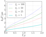
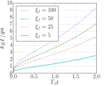
Figure 1: Evolution of the temperature of a 3D weakly interacting Bose-Einstein condensate under the effect of losses. Temperature is rescaled to the time-dependent chemical potential $\mu\simeq gn\simeq gn_{0}e^{-\Gamma_{0}t}$, where $n$ is the atomic density, equal to $n_{0}$ at $t=0$, $g$ the interaction strength and $\Gamma_{0}$ is the single atom loss rate. The initial value is $k_{B}T(0)/(gn_{0})=0.1$. In (a) interactions are contact interactions but the reservoir has a finite energy width $E_{\rm res}$, parameterized by the dimensionless parameter $\xi_{1}=\sqrt{E_{\rm res}/(gn_{0})}$. In (b), we assume a reservoir of infinite energy width, or equivalently of vanishing correlation time, but interactions have a finite range $\sigma$ (see text) and $\xi_{2}=\hbar/(\sigma\sqrt{mgn_{0}})$.

The system is ergodic in dimension $d>1$: beyond Bogoliubov terms in $H_{0}$ include couplings between Bogoliubov modes which, in absence of losses and as long as local observables are concerned, ensure relaxation towards a thermal state. Here we assume that $\Gamma_{0}$ is much smaller than the relaxation rate so that, $\hat{\rho}$ relaxes at any time to the density matrix of a thermal state. The latter is characterized by the atomic density $n$ and the energy density, or equivalently by $n$ and the temperature $T$. The energy of the gas fulfills $E=E_{\rm th}(n,T)$, where $E_{\rm th}(n,T)$ is evaluated injecting the occupation factors $\langle a_{\bf p}^{+}a_{\bf p}\rangle=(e^{\epsilon_{p}/(k_{B}T)}-1)^{-1}$ into Eq. (9). The time evolution of the gas is entirely characterized by the functions $n(t)=n_{0}e^{-\Gamma_{0}t}$ and $T(t)$. In order to compute $T(t)$, we evaluate $dT/dt$ in the following way. Since $E$ is conserved by the thermalization process, the calculation of $dE/dt$ with Eq. (13) and (14) is valid, providing one injects $\langle a_{\bf p}^{+}a_{\bf p}\rangle=(e^{\epsilon_{p}/(k_{B}T)}-1)^{-1}$ in the r.h.s of Eq. (14). Once $dE/dt$ has been computed one can compute $dT/dt$ using $dE/dt=-\Gamma_{0}n(\partial E_{\rm th}/\partial n)_{T}+dT/dt(\partial E_{\rm th}/\partial T)_{n}$. Calculations are detailed in the appendix.

In Fig. 1 we present time evolution of the temperature of the system, for different values of $E_{\rm res}$. We find that the ratio $k_{B}T/(gn)$ is a growing function of time. This contrasts with the prediction obtained for phonons, which are the Bogoliubov modes of momentum $p\ll\sqrt{mgn}$ : in absence of rethermalization between Bogoliubov modes, and for $E_{\rm res}\gg gn$, one expects that, for phonons, $k_{B}T/(gn)$ takes the asymptotic value $k_{B}T/(gn)=1$ Grišins et al. (2016); Johnson et al. (2017). The growing of $k_{B}T/gn$ is due to the contribution of high-$p$ Bogoliubov modes. The growing rate increases with $E_{\rm res}$, as expected: we expect that $dT/dt$ diverges as $E_{\rm res}$ goes to infinity.

Regularization by a finite interaction range.

The Bogoliubov analysis can serve also to describe the regularization of the UV divergence due to finite interaction range. We consider here a two-body interaction potential $V(r)=ge^{-r^{2}/(2\sigma^{2})}/((2\pi)^{3/2}\sigma^{3})$, where $r$ is the distance between the two atoms and $\sigma$ is the interaction range. The Bogoliubov transform given in Eq. (10) is still valid, using the Bogoliubov spectrum Bogolubov (2014) $\epsilon_{\bf p}=\sqrt{p^{2}/(2m)(p^{2}/(2m)+2gne^{-p^{2}\sigma^{2}/(2\hbar^{2})})}$. One can then compute the effect of losses as above. In the limit of infinite $E_{\rm res}$, the divergence of $dE/dt$ is regularized by the finite interaction range $\sigma$. For very small $\sigma$, $dE/dt$ is dominated by the large $p$ term of the sum in Eq. (13), for which $v_{p}^{2}\simeq(mgn)^{2}(e^{-p^{2}\sigma^{2}/\hbar^{2}})/p^{4}$. Evaluating the sum, we recover Eq. (8) with ${\cal B}=\pi^{3/2}\hbar/\sigma$. As above, from the calculation of $dE/dt$ due to losses, we compute the time evolution of the temperature in the system. Fig. 1 shows the time evolution of the temperature, for different values of $\sigma$. The evolution of $k_{B}T/(gn)$ is qualitatively similar to what is observed for contact interactions but finite energy width of the reservoir, $\hbar^{2}/(m\sigma^{2})$ playing the role of $E_{\rm res}$.

Conclusion.

Remarkably, although losses are ubiquitous in experiments, the description and the understanding of their effect is still at its infancy. Before this work, effect of losses has been studied using the universal Lindblad equation Eq. (1). However, studies where made either in 1D, in which case the divergence of the energy increase rate does not exists, or for a gas confined in the lowest band of a lattice, in which case the lattice period provides a cut-off that prevents the divergence, or using a mean-field approximation that neglect correlations between atoms. This paper provides the first prediction for the effect of losses on an interacting quantum gas in higher dimension and in the continuum. Predictions of this paper could be tested experimentally using an engineered noisy coupling to an untrapped state Bouchoule and Schemmer (2020) whose energy width $E_{\rm res}$ can be varied. This work raises many questions. How can we extend the results obtained with Bogoliubov to quasi-condensate describing 2D gases at thermodynamic limit ? How can the results presented in this paper be extended to 2-body or 3-body losses ? How can we extend the calculations done in this paper to other models of quantum gases, such as two-components fermionic gases ?

Appendix A Single-atom case: loss rate

Let us assume that the system comprises, at $t=0$, a single atom of momentum ${\bf p}$. After an evolution time $t$, the state of the system writes $c_{0}e^{-itp^{2}/(2\hbar m)}\Psi^{+}_{\bf p}|0\rangle+c_{1}e^{-itp^{2}/(2\hbar m)}B_{\bf p}^{+}|0\rangle$, where $c_{0}(t=0)=1$ and $c_{1}(t=0)=0$. Using perturbation theory, one has $c_{1}(t)=-i\int_{0}^{t}d\tau\Omega(\tau)$ such that

$$|c_{1}(t)|^{2}=\frac{1}{\hbar^{2}}\int_{0}^{t}\int_{0}^{t}d\tau_{1}d\tau_{2}\Omega^{*}(\tau_{1})\Omega(\tau_{2}).$$ (15)

For weak enough $\Omega$, the evolution of $c_{1}(t)$ and $c_{0}(t)$ are slow enough so that one can consider times $t$ both much larger than the correlation time of $\Omega$ and small enough so that $c_{0}$ barely changed and the above perturbation calculation holds. This is the so called Born-Markov approximation, under which Eq. (15) writes

$$|c_{1}(t)|^{2}=t\int_{-\infty}^{\infty}d\tau\langle\Omega^{*}(0)\Omega(\tau)\rangle=t\Gamma_{0}.$$ (16)

Thus, the loss rate is $\Gamma_{0}$. It does not depends on the momentum of the atom. The above calculation is similar to the usual Fermi Golden Rule calculation, the different Fourier components of $\Omega$ playing the role of the different states of the continuum. Note that the fact the energy of the state $B_{\bf p}|0\rangle$ is $p^{2}/(2m)$ ensures Galilean invariance of the loss process: the loss rate does not dependent on ${\bf p}$, as expected since one can compute the loss rate in the moving frame where ${\bf p}={\bf 0}$.

Appendix B Two-atom case: loss rate towards $|{\bf p}\rangle$

Here we assume the system initially comprises 2 atoms. The loss rate towards a state $|{\bf p}\rangle$, given in Eq. (5), is computed using a similar calculation as in the above appendix. The initial state $|\varphi\rangle$ is coupled by $V$ to the final states $|{\bf p}\rangle$ and the state of the system at time $t$ writes $c_{0}e^{-iE_{0}t/\hbar}|\varphi\rangle+\sum_{\bf p}c_{\bf p}e^{-itp^{2}/(\hbar m)}|{\bf p}\rangle$, where $c_{0}(t=0)=1$ and $c_{\bf p}(t=0)=0$. Using perturbation theory, one has $c_{\bf p}(t)=-i\varphi({\bf p})\int_{0}^{t}d\tau\Omega(\tau)e^{i(p^{2}/m-E_{0})\tau/\hbar}$ such that the population in the state $|{\bf p}\rangle$ at time $t$ writes

$$|c_{\bf p}(t)|^{2}=\frac{|\varphi({\bf p})|^{2}}{\hbar^{2}}\int_{0}^{t}\int_{0}^{t}d\tau_{1}d\tau_{2}\Omega^{*}(\tau_{1})\Omega(\tau_{2})e^{i(p^{2}/m-E_{0})(\tau_{2}-\tau_{1})/\hbar}.$$ (17)

We then make the Born-Markov approximation as in the above appendix: for weak enough $\Omega$, the evolution of $c_{\bf p}(t)$ and $c_{0}(t)$ are slow enough so that one can consider times $t$ both much larger than the correlation time of $\Omega$ and small enough so that $c_{0}$ barely changed and the above perturbation calculation holds. Eq. (17) then transforms into

$$|c_{\bf p}(t)|^{2}=t|\varphi({\bf p})|^{2}\int_{-\infty}^{\infty}d\tau\langle\Omega^{*}(0)\Omega(\tau)\rangle e^{i(p^{2}/m-E_{0})\tau/\hbar}.$$ (18)

We thus recover Eq. (5) using $\gamma({\bf p})=|c_{\bf p}(t)|^{2}/t$.

Appendix C Noisy time-dependent coupling versus coupling to a reservoir

In this paper, for simplicity of notations, instead of considering a reservoir where losses occur – i.e. a continuum of states–, we consider a fluctuating time dependent coupling towards a secondary internal state. This would correspond for instance to a coupling to a different zeeman state by a noisy magnetic field, as done in Bouchoule and Schemmer (2020). The different Fourier components of the coupling play the role of the different states of a reservoir, as shown below.

In this appendix we consider a time-independent coupling towards a reservoir. The states of the reservoir in which an atom of the system can decay write $|{\bf p},i\rangle_{\cal R}=B^{+}_{{\bf p},i}|0\rangle$: they are labeled by their momentum ${\bf p}$ and an additional index $i$ which, in a discretized representation, labels the states of the continuum. For instance, atoms in 2D, confined to the ground state of a vertical confining potential, could be coupled to states untrapped in the vertical direction and $i$ labels the vertical momentum of the free atoms. In 3D, in the case of metastable atoms decaying to an untrapped state with the emission of a photon, $i$ would label the momentum of the emitted photon. The coupling between the system and the reservoir writes

$$V=\sum_{{\bf p},i}V_{i}\Psi_{\bf p}B^{+}_{{\bf p},i}+h.c..$$ (19)

The fact that the coupling $V_{i}$ does not depend on ${\bf p}$ ensures a homogeneous loss process. The energy of the states $|{\bf p},i\rangle_{\cal R}$ are $E_{{\bf p},i}=p^{2}/(2m)+E_{i}$, which ensures invariance by Galilean transformation.

To make the correspondence with the noisy loss model used in the main text, let us consider the situation where the initial state comprises 2 atoms in the system. After an evolution time $t$, the population in the states of the reservoir of momentum ${\bf p}$, evaluated using second order theory is

$$P_{\bf p}(t)=|\varphi({\bf p})|^{2}\sum_{i}\int_{0}^{t}\int_{0}^{t}d\tau_{1}d\tau_{2}\frac{|V_{i}|^{2}}{\hbar^{2}}e^{i(E_{i}+p^{2}/m-E_{0})(\tau_{1}-\tau_{2})/\hbar}.$$ (20)

Let us introduce the function

$${\cal R}(\tau)=\sum_{i}|V_{i}|^{2}e^{iE_{i}\tau}$$ (21)

whose width, denoted $\tau_{c}$, is called the correlation time of the reservoir. We assume losses are weak enough so that the typical time of decrease of the initial state population is much larger than $\tau_{c}$. Then, one can consider times $t$ both small enough so that the population in the initial state barely changed and large enough to fulfill $t\gg\tau_{c}$. This is the Born-Markov approximation, which permits to writes Eq. (20) as

$$P_{\bf p}(t)=t|\varphi({\bf p})|^{2}\int_{-\infty}^{\infty}d\tau{\cal R}(\tau)e^{i(p^{2}/m-E_{0})\tau}.$$ (22)

We thus recover Eq. (18), providing we make the identification

$${\cal R}(\tau)\iff\langle\Omega^{*}(0)\Omega(\tau)\rangle.$$ (23)

In the frequency domain, the correspondence between the time-dependent noisy coupling and the coupling to the reservoir reads

$$2\pi n(E)|V(E)|^{2}/\hbar\iff\Gamma(-E).$$ (24)

where $V(E)$ is the value of $V_{i}$ for states at an energy $E_{i}\simeq E$ and $n(E)=\sum_{i}\delta(E_{i}-E)$ is the density of state of the reservoir.

Here we established the equivalence between a noisy time-dependent coupling and a time-independent coupling towards a reservoir for the short time dynamics. For the dynamics to be equivalent at longer times, the secondary internal state towards which atoms are transferred by the noisy function $\Omega(t)$ should actually be removed, on a typical time short compared to the typical evolution time of the system. This will be the case if they are untrapped and quit the zone where the atoms of the system are trapped. If the removal time is much larger than the correlation time of $\Omega(t)$, the loss process will be correctly captured by the model presented in the main text: the relevant energy width for the loss process is the energy width of the function $\Gamma(E)$ given Eq. (3) of the main text, which is nothing else than $\hbar/\tau_{c}$ where $\tau_{c}$ is the correlation time of $\Omega$.

Note finally that the choice of a model of losses based on a noisy time-dependent function is not essential for the results presented in this paper. The master equation given Eq. (12) of the main text, derived in the appendix below for losses induced by a noisy time-dependent coupling, could also be derived using the coupling to a reservoir given in Eq. (19), at the price of slightly more complicated notations. At the end, one would recover the same results using the correspondence of Eq. (23) and Eq. (24).

Appendix D Derivation of the master equation

Let us first consider the system that comprises both the gas under study and the environment in which losses occur. Its density matrix is noted $\rho_{\Sigma}$ and its Hamiltonian writes $H_{\Sigma}=H_{0}+H_{\mathrm{Res}}+V$, where $H_{0}$ is the Hamiltonian of the quantum gas, $H_{\mathrm{Res}}$ is the Hamiltonian of the reservoir and $V$ is the coupling Hamiltonian between the quantum gas and the reservoir. As explained in the main text, we use the Bogoliubov approximation to describe the quantum gas. At time $t$, we assume there is no correlation between the environment and the system such that $\rho_{\Sigma}(t)=\rho(t)\otimes|0_{R}><0_{R}|$.

We work in the interaction representation, in which an operator $A$ writes $\tilde{A}(t)=e^{i(H_{0}+H_{\mathrm{Res}})\frac{t}{\hbar}}Ae^{-i(H_{0}+H_{\mathrm{Res}})\frac{t}{\hbar}}$, where $A$ is the operator in the Shrödinger picture. The evolution of the density matrix $\tilde{\rho}_{\Sigma}$ is given by

$$i\hbar\frac{\mathrm{d}\tilde{\rho}_{\Sigma}}{\mathrm{d}t}=[\tilde{V},\tilde{\rho}_{\Sigma}].$$ (25)

We consider the evolution of $\tilde{\rho}_{\Sigma}$ on a time $\delta t$ small enough so that we can restrain to second order perturbation theory. Integration of the above equation then leads to

$$\tilde{\rho}_{\Sigma}(t+\delta t)=\tilde{\rho}_{\Sigma}(t)+\frac{1}{i\hbar}\int_{t}^{t+\delta t}[\tilde{V}(\tau),\tilde{\rho}_{\Sigma}(t)]\mathrm{d}\tau-\frac{1}{\hbar^{2}}\int_{t}^{t+\delta t}\mathrm{d}\tau\int_{t}^{\tau}\mathrm{d}\tau^{\prime}[\tilde{V}(\tau),[\tilde{V}(\tau^{\prime}),\tilde{\rho}_{\Sigma}(t)]]$$ (26)

The coupling $\tilde{V}(t)$ is obtained from its Shrödinger representation given in Eq. (2) of the main text, using the interaction representation of the operators. The latter are obtained from

$$\left\{\begin{array}[]{lll}\tilde{B}_{\mathbf{p}}&=e^{-i\omega_{\mathbf{p}}^{\mathrm{Res}}t}B_{\mathbf{p}}&\mbox{with}\;\omega_{\mathbf{p}}^{\mathrm{Res}}=(p^{2}/(2m)-gn)\hbar\\ \tilde{a}_{\mathbf{p}}&=e^{-i\omega_{\mathbf{p}}t}a_{\mathbf{p}}&\mbox{with}\;\omega_{\mathbf{p}}=\epsilon_{p}/{\hbar}.\end{array}\right.$$ (27)

where the $\epsilon_{p}=\sqrt{p^{2}/(2m)(p^{2}/(2m)+2gn)}$ is the energy of the Bogoliubov mode of momentum ${\bf p}$. The term $gn=\partial E_{0}/\partial N$ amount to the energy shift of the ground state energy of the gas when an atom is removed from the system. It is taken into account by a shift in energy of the reservoir states. The validity of this approach appears if one consider a number-preserving Bogoliubov approach where Bogoliubov operators conserve atom-number Castin and Dum (1998). In this approach, the operator $B_{\bf p}^{+}$ ( resp. $B_{\bf p}$) in $V$ would be replaced by the operator $\Lambda B_{\bf p}^{+}$ (resp. $\Lambda^{+}B_{\bf p}p$) where $\Lambda\simeq(1\sqrt{N})\Psi_{\bf 0}$ remove an atom from the condensate.

We are interested in computing the state of the gas at time $t+\delta t$, irrespective of the state of the reservoir. We thus trace over the reservoir and compute $\tilde{\rho}=Tr_{\mathrm{Res}}(\tilde{\rho}_{\Sigma})$. Tracing out the reservoir degrees of freedom in Eq. (26), doing the variable change $u=\tau-\tau^{\prime}$, and using the fact that the reservoir is in its empty state at time $t$, we obtain

$$\tilde{\rho}(t+\delta t)=\tilde{\rho}(t)-\frac{1}{\hbar^{2}}\sum_{\mathbf{p}}\int_{t}^{t+\delta t}\mathrm{d}\tau\int_{0}^{\tau}du\left\{\Omega^{*}(\tau)\Omega(\tau-u)[A_{\mathbf{p}}^{(1)}(u)+A_{\mathbf{p}}^{(2)}(\tau,u)]+h.c.\right\}$$ (28)

with

$$A_{\mathbf{p}}^{(1)}(u)=u_{\mathbf{p}}^{2}e^{i(\omega_{\mathbf{p}}-\omega_{\mathbf{p}}^{\mathrm{Res}})u}\left({a}_{\mathbf{p}}^{+}{a}_{\mathbf{p}}\tilde{\rho}(t)-{a}_{\mathbf{p}}\tilde{\rho}(t){a}_{\mathbf{p}}^{+}\right)+v_{\mathbf{p}}^{2}e^{-i(\omega_{\mathbf{p}}^{\mathrm{Res}}+\omega_{\mathbf{p}})u}\left({a}_{-\mathbf{p}}{a}_{-\mathbf{p}}^{+}\tilde{\rho}(t)-{a}_{-\mathbf{p}}^{+}\tilde{\rho}(t){a}_{-\mathbf{p}}\right)\\$$ (29)

and

$$A_{\mathbf{p}}^{(2)}(\tau,u)=u_{\mathbf{p}}v_{\mathbf{p}}[e^{-i2\omega_{\mathbf{p}}\tau}e^{-i(\omega_{\mathbf{p}}^{\mathrm{Res}}-\omega_{\bf p})u}({a}_{\mathbf{-p}}{a}_{\mathbf{p}}\tilde{\rho}(t)-{a}_{\mathbf{p}}\tilde{\rho}(t){a}_{-\mathbf{p}})+e^{i2\omega_{\mathbf{p}}\tau}e^{-i(\omega_{\mathbf{p}}^{\mathrm{Res}}+\omega_{\bf p})u}({a}_{\mathbf{p}}^{+}{a}_{-\mathbf{p}}^{+}\tilde{\rho}(t)-{a}_{\mathbf{-p}}^{+}\tilde{\rho}(t){a}_{\mathbf{p}}^{+})]$$ (30)

The term $A_{\mathbf{p}}^{(2)}$ oscillates in $\tau$ with the frequency $2\omega_{\bf p}$. Since losses are weak, we expect that $\tilde{\rho}$ evolves slowly compared to $\omega_{\bf p}$. Thus, the effect of $A_{\mathbf{p}}^{(2)}$ will average out. In the following we neglect this term. This constitutes a secular approximation, also called a rotating wave approximation.

To compute the effect of the term $A_{\mathbf{p}}^{(1)}$, we use a Born-Markov approximation. This approximation holds assuming the losses are weak enough so that the time evolution of $\tilde{\rho}$ occurs on times much larger than the correlation time of $\Omega$, noted $\tau_{c}$. Then one can consider a time interval $\delta t$ large enough so that that $\delta t\gg\tau_{c}$ but small enough so that the evolution of $\tilde{\rho}$ is small and the second order calculation is valid. The condition $\delta t\gg\tau_{c}$ permit to write Eq. (28) as

$$\tilde{\rho}(t+\delta t)=\tilde{\rho}(t)-\frac{\delta t}{\hbar^{2}}\sum_{\mathbf{p}}\left(\int_{0}^{\infty}du\langle\Omega^{*}(0)\Omega(-u)\rangle A_{\mathbf{p}}^{(1)}(u)+h.c.\right).$$ (31)

Injecting Eq. (29) into the above integral, one finds integrals of the form $\int_{0}^{\infty}du\langle\Omega^{*}(0)\Omega(-u)\rangle e^{-i\nu u}$, where $\nu=\omega_{\mathbf{p}}^{\mathrm{Res}}\pm\omega_{\bf p}$. We write them as $\hbar^{2}\Gamma(\nu)/2+i{\cal I}m(\int_{0}^{\infty}du\langle\Omega^{*}(0)\Omega(-u)\rangle e^{-i\nu u})$, where the function $\Gamma(E)$ is defined in Eq. (3) of the main text. We then use the fact that $\delta t$ is small compared to the evolution time of $\tilde{\rho}$, such that $d\tilde{\rho}/dt=(\tilde{\rho}(t+\delta t)-\tilde{\rho}(t))/\delta t$. Finally, Eq. (31) gives

$$\begin{split}\frac{\mathrm{d}}{\mathrm{d}t}\tilde{\rho}(t)=-\sum_{\mathbf{p}}\left\{\right.&\Gamma(\frac{\mathbf{p}^{2}}{2m}-gn-\epsilon_{\mathbf{p}})u_{\mathbf{p}}^{2}(\frac{1}{2}\{a_{\mathbf{p}}^{{\dagger}}a_{\mathbf{p}},\tilde{\rho}(t)\}-a_{\mathbf{p}}\tilde{\rho}(t)a_{\mathbf{p}}^{{\dagger}})\\ &+\Gamma(\frac{\mathbf{p}^{2}}{2m}-gn+\epsilon_{\mathbf{p}})v_{\mathbf{p}}^{2}(\frac{1}{2}\{a_{\mathbf{p}}a_{\mathbf{p}}^{{\dagger}},\tilde{\rho}(t)\}-a_{\mathbf{p}}^{{\dagger}}\tilde{\rho}(t)a_{\mathbf{p}})\\ &-i\left.\left[\Delta_{p}+\Delta_{p}^{\prime}a^{+}_{\bf p}a_{\bf p},\tilde{\rho}\right]\right\}\end{split}$$ (32)

where the commutator term, which corresponds to the effect of an hermitian term, comes from the integrals in ${\cal I}m(\int_{0}^{\infty}du\langle\Omega^{*}(0)\Omega(-u)\rangle e^{-i\nu u})$ and amounts to the Lamb shift effect. It corresponds to a small correction of the energies of the Bogoliubov modes, that we neglect in the following. Going back to the Shrödinger picture, we recover the master equation given in Eq. (12) of the main text.

Eq. (12) of the main text takes the form of a Lindblad equation. The originality in the above derivation is that the Born-Markov approximation can be done only after the rotating wave approximation has been used to eliminate non resonant terms corresponding to the term (30). The Born-Markov approximation cannot be done before such an approximation since we might consider Bogoliubov modes whose frequencies $\omega_{\bf p}$ can be as large or higher than the reservoir frequency width $1/\tau_{c}$.

In the above derivation of the master equation, we used a model of losses based on a time-dependent noisy function. This permits to have simple expressions. One could reproduce such calculations using instead a time-independent coupling towards a continuum of state, such as the model considered in the appendix B.

Appendix E Adiabatic following of $\langle a^{+}_{\bf p}a_{\bf p}\rangle$

The Bogoliubov transformation given Eq. (10) of the main text invert into

$$\left\{\begin{array}[]{l}a_{\bf p}=u_{p}\Psi_{\bf p}-v_{p}\Psi^{+}_{-\bf p}\\ a^{+}_{\bf p}=u_{p}\Psi^{+}_{\bf p}-v_{p}\Psi_{-\bf p}\\ \end{array}\right.$$ (33)

The decrease of $n$ due to the loss process makes the functions $u_{p}$ and $v_{p}$ time dependent and we note $\dot{u_{p}}=du_{p}/dt$ and $\dot{v_{p}}=dv_{p}/dt$. Thus the operator $a^{+}_{\bf p}a_{\bf p}$ depends on time. Computing $d(a^{+}_{\bf p}a_{\bf p})/dt$ using the Bogoliubov transforms, and using the fact that, since $u_{p}^{2}-v_{p}^{2}=1$ for any time, $\dot{u}_{p}u_{p}-\dot{v_{p}}v_{p}=0$, we obtain

$$\langle d(a^{+}_{\bf p}a_{\bf p})/dt\rangle=(\dot{u}_{p}v_{p}-\dot{v}_{p}u_{p})\left(\langle a_{-{\bf p}}a_{\bf p}\rangle+\langle a^{+}_{-{\bf p}}a^{+}_{\bf p}\rangle\right)$$ (34)

The mean values on the right hand side typically oscillate at the frequency $2\epsilon_{p}/\hbar$. On the other hand we assume slow losses such that the evolution rate of $u_{p}$ and $v_{p}$ are much smaller than $\epsilon_{p}/\hbar$, and the evolution of $\langle a^{+}_{\bf p}a_{\bf p}\rangle$ is also expected to occur on time scales much longer than $\hbar/\epsilon_{p}$. Making a coarse grained approximation in time domain, the above equation then reduces to

$$\langle d(a^{+}_{\bf p}a_{\bf p})/dt\rangle\simeq 0.$$ (35)

This approximation is a rotating wave approximation similar to that used in the above appendix to derive the master equation.

Appendix F Time evolution of the temperature of the system

We assume slow enough losses so that the gas has time to relax, at each time, towards a thermal state, parameterized by the density $n$ and the temperature $T$. The energy of the gas at time $t$ is $E(t)=E_{\rm th}(n(t),T(t))$ where $E_{\rm th}(n,T)$, evaluated using the Bogoliuobv expression given in Eq. (9) of the main text, is

$$E_{\rm th}(n,T)=e_{0}L^{d}+\sum_{{\bf p}\neq{\bf 0}}\epsilon_{p}n_{B}(\epsilon_{\bf p},T)$$ (36)

where

$$n_{B}(\epsilon,T)=\left(e^{\epsilon/T}-1\right)^{-1}$$ (37)

is the Bose occupation factor of a mode of energy $\epsilon$. The $n$-dependence of $E_{\rm th}$ comes from the $n$-dependence of $e_{0}$ and $\epsilon_{p}$, and its dependence on $T$ comes from the $T$-dependence of the Bose occupation factors.

The density evolves as $dn/dt=-\Gamma_{0}n$. This expression is exact when the time correlation of the reservoir is vanishing, and it is a very good approximation for reservoir of finite energy width as long as the energy width is large enough. One is then left in computing the time evolution of the temperature. The time derivative of $T$ is linked to $dE/dt$ as

$$\frac{dE}{dt}=\left(\frac{\partial E_{\rm th}}{\partial n}\right)_{T}(-\Gamma_{0}n)+\left(\frac{\partial E_{\rm th}}{\partial T}\right)_{n}\frac{dT}{dt},$$ (38)

which gives

$$\begin{split}\frac{dE}{dt}=&-\Gamma_{0}nL^{d}\frac{de_{0}}{dn}-\Gamma_{0}n\sum_{\bf p}\frac{d\epsilon_{p}}{dn}\left(n(\epsilon_{p},T)+\epsilon_{p}\frac{\partial n_{B}(\epsilon_{p},T)}{\partial\epsilon_{p}}\right)\\ &+\frac{dT}{dt}\sum_{\bf p}\epsilon_{p}\frac{dn_{B}(\epsilon_{p},T)}{dT}\end{split}$$ (39)

On the other hand, in the main text, $dE/dt$ is computed within the Bogoliubov theory and using the master equation describing the effect of losses. The result is given by Eq. (13) and Eq. (14) of the main text, where one should evaluate Eq. (14) using for $\langle a^{+}_{p}a_{p}\rangle$ the thermal occupation factors given in Eq. (37). Comparing with Eq. (39), and calculating explicitly the partial derivatives of $n_{B}$, we find that $dT/dt$ fulfills

$$\frac{dT}{dt}\sum_{\bf p}\frac{\epsilon_{\bf p}^{2}}{k_{B}T^{2}}\frac{e^{\epsilon_{\bf p}/k_{B}T}}{(e^{\epsilon_{\bf p}/k_{B}T}-1)^{2}}=\sum_{\bf p}\epsilon_{\bf p}\left\{\left(\frac{d\langle a_{\bf p}^{+}a_{\bf p}\rangle}{dt}\right)_{BG}-\Gamma_{0}n\frac{\epsilon_{p}}{(k_{B}T)^{2}}\frac{e^{\epsilon_{p}/T}}{(e^{\epsilon_{p}/T}-1)^{2}}\frac{\partial\epsilon_{p}}{\partial n}\right\}$$ (40)

where $\left({d\langle a_{\bf p}^{+}a_{\bf p}\rangle}/{dt}\right)_{BG}$ is evaluated from Eq. (14) of the main text, injecting the thermal Bose occupation factors $\langle a^{+}_{\bf p}a_{\bf p}\rangle=n_{B}(\epsilon_{p},T)$.

We can apply this result in the two cases considered in the article. In the case of contact interactions but a reservoir of finite energy width, $dT/dt$ is computed by injecting $d\epsilon_{p}/dn=gp^{2}/(2m)/\epsilon_{p}$. In the case of a reservoir of infinite energy width but for finite range interactions, $dT/dt$ is computed by injecting $d\epsilon_{p}/dn=ge^{-p^{2}\sigma^{2}/2}p^{2}/(2m)/\epsilon_{p}$. Note also that in this case, Eq. (14) of the main text simplifies to $\left({d\langle a_{\bf p}^{+}a_{\bf p}\rangle}/{dt}\right)_{BG}=-\Gamma_{0}(n_{B}(\epsilon_{p},T)+v_{p}^{2})$.

References

- Diehl et al. (2008) S. Diehl, A. Micheli, A. Kantian, B. Kraus, H. P. Büchler, and P. Zoller, Nature Physics 4, 878 (2008).
- Poletti et al. (2013) D. Poletti, P. Barmettler, A. Georges, and C. Kollath, Phys. Rev. Lett. 111, 195301 (2013), publisher: American Physical Society.
- Barreiro et al. (2011) J. T. Barreiro, M. Müller, P. Schindler, D. Nigg, T. Monz, M. Chwalla, M. Hennrich, C. F. Roos, P. Zoller, and R. Blatt, Nature 470, 486 (2011), number: 7335 Publisher: Nature Publishing Group.
- Verstraete et al. (2009) F. Verstraete, M. M. Wolf, and J. Ignacio Cirac, Nature Physics 5, 633 (2009), number: 9 Publisher: Nature Publishing Group.
- Roncaglia et al. (2010) M. Roncaglia, M. Rizzi, and J. I. Cirac, Phys. Rev. Lett. 104, 096803 (2010), publisher: American Physical Society.
- Kantian et al. (2009) A. Kantian, M. Dalmonte, S. Diehl, W. Hofstetter, P. Zoller, and A. J. Daley, Phys. Rev. Lett. 103, 240401 (2009), publisher: American Physical Society.
- Foss-Feig et al. (2012) M. Foss-Feig, A. J. Daley, J. K. Thompson, and A. M. Rey, Phys. Rev. Lett. 109, 230501 (2012), publisher: American Physical Society.
- Syassen et al. (2008) N. Syassen, D. M. Bauer, M. Lettner, T. Volz, D. Dietze, J. J. García-Ripoll, J. I. Cirac, G. Rempe, and S. Dürr, Science 320, 1329 (2008), publisher: American Association for the Advancement of Science Section: Report.
- Barontini et al. (2013) G. Barontini, R. Labouvie, F. Stubenrauch, A. Vogler, V. Guarrera, and H. Ott, Phys. Rev. Lett. 110, 035302 (2013).
- Nakagawa et al. (2021) M. Nakagawa, N. Kawakami, and M. Ueda, Phys. Rev. Lett. 126, 110404 (2021), publisher: American Physical Society.
- García-Ripoll et al. (2009) J. J. García-Ripoll, S. Dürr, N. Syassen, D. M. Bauer, M. Lettner, G. Rempe, and J. I. Cirac, New J. Phys. 11, 013053 (2009), publisher: IOP Publishing.
- Labouvie et al. (2016) R. Labouvie, B. Santra, S. Heun, and H. Ott, Phys. Rev. Lett. 116, 235302 (2016), publisher: American Physical Society.
- Johnson et al. (2017) A. Johnson, S. S. Szigeti, M. Schemmer, and I. Bouchoule, Phys. Rev. A 96, 013623 (2017).
- Bouchoule et al. (2020) I. Bouchoule, B. Doyon, and J. Dubail, (2020).
- Rossini et al. (2020) D. Rossini, A. Ghermaoui, M. B. Aguilera, R. Vatré, R. Bouganne, J. Beugnon, F. Gerbier, and L. Mazza, arXiv:2011.04318 [cond-mat] (2020), arXiv: 2011.04318.
- Bouchoule and Dubail (2021) I. Bouchoule and J. Dubail, Phys. Rev. Lett. 126, 160603 (2021), publisher: American Physical Society.
- Rauer et al. (2016) B. Rauer, P. Grišins, I. Mazets, T. Schweigler, W. Rohringer, R. Geiger, T. Langen, and J. Schmiedmayer, Phys. Rev. Lett. 116, 030402 (2016).
- Schemmer and Bouchoule (2018) M. Schemmer and I. Bouchoule, Phys. Rev. Lett. 121, 200401 (2018).
- Bouchoule and Schemmer (2020) I. Bouchoule and M. Schemmer, SciPost Physics 8, 060 (2020).
- Daley (2014) A. J. Daley, Advances in Physics 63, 77 (2014), publisher: Taylor & Francis _eprint: https://doi.org/10.1080/00018732.2014.933502.
- Werner and Castin (2012a) F. Werner and Y. Castin, Phys. Rev. A 86, 013626 (2012a), publisher: American Physical Society.
- (22) See Supplemental Material for () the calculation of the loss rate for a single atom, () the derivation of formula (5), () the derivation of the equivalence between a noisy time-dependent coupling and a couling to a continuum of states, () the derivation of the master equation Eq. (12), the justification of the fact that is not affected by the slow time-variation of and , and the calculation of the time-evolution of the temperature.
- Werner and Castin (2012b) F. Werner and Y. Castin, Phys. Rev. A 86, 053633 (2012b), publisher: American Physical Society.
- Tan (2008) S. Tan, Annals of Physics 323, 2952 (2008).
- Note (1) See appendix C of the Supplemental material for a discussion on this point.
- Note (2) See the appendix B of Johnson et al. (2017).
- Grišins et al. (2016) P. Grišins, B. Rauer, T. Langen, J. Schmiedmayer, and I. E. Mazets, Phys. Rev. A 93, 033634 (2016).
- Bogolubov (2014) N. N. Bogolubov, Jr., Quantum Statistical Mechanics: Selected Works of N N Bogolubov (WORLD SCIENTIFIC, 2014).
- Castin and Dum (1998) Y. Castin and R. Dum, Phys. Rev. A 57, 3008 (1998).